Casimir Interactions between Magnetic Flux Tubes in a Dense Lattice

Dan Mazur Email: daniel.mazur@mcgill.ca Affiliation: McGill High Performance Computing Centre, McGill University, 1100 Rue Notre-Dame Ouest, Montreal, QC H3C 1K3 Jeremy S. Heyl Email: heyl@phas.ubc.ca Affiliation: Department of Physics and Astronomy, University of British Columbia, Vancouver BC V6T 1Z1 Canada; Canada Research Chair

Abstract

We use the worldline numerics technique to study a cylindrically symmetric model of magnetic flux tubes in a dense lattice and the non-local Casimir forces acting between regions of magnetic flux. Within a superconductor the magnetic field is constrained within magnetic flux tubes and if the background magnetic field is on the order the quantum critical field strength, $B_{k}=\frac{m^{2}}{e}=4.4\times 10^{13}$ Gauss, the magnetic field is likely to vary rapidly on the scales where QED effects are important. In this paper, we construct a cylindrically symmetric toy model of a flux tube lattice in which the non-local influence of QED on neighbouring flux tubes is taken into account. We compute the effective action densities using the worldline numerics technique. The numerics predict a greater effective energy density in the region of the flux tube, but a smaller energy density in the regions between the flux tubes compared to a locally-constant-field approximation. We also compute the interaction energy between a flux tube and its neighbours as the lattice spacing is reduced from infinity. Because our flux tubes exhibit compact support, this energy is entirely non-local and predicted to be zero in local approximations such as the derivative expansion. This Casimir-Polder energy can take positive or negative values depending on the distance between the flux tubes, and it may cause the flux tubes in neutron stars to form bunches.

In addition to the above results we also discuss two important subtleties of determining the statistical uncertainties within the worldline numerics technique. Firstly, the distributions generated by the worldline ensembles are highly non-Gaussian, and so the standard error in the mean is not a good measure of the statistical uncertainty. Secondly, because the same ensemble of worldlines is used to compute the Wilson loops at different values of $T$ and $x_{\mathrm{cm}}$ , the uncertainties associated with each computed value of the integrand are strongly correlated. We recommend a form of jackknife analysis which deals with both of these problems.

I Introduction

In this contribution, we make use of a numerical technique which can be used to compute the effective actions of external field configurations. The technique, called either worldline numerics or the Loop-Cloud Method, was first used by Gies and Langfeld [1] and has since been applied to computation of effective actions [2, 3, 4, 5, 6] and Casimir energies [7, 8, 9]. More recently, the technique has also been applied to pair production [10] and the vacuum polarization tensor [11]. Worldline numerics is able to compute quantum effective actions in the one-loop approximation to all orders in both the coupling and in the external field, so it is well suited to studying non-perturbative aspects of quantum field theory in strong background fields. Moreover, the technique maintains gauge invariance and Lorentz invariance. The key idea of the technique is that a path integral is approximated as the average of a finite set of $N_{l}$ representative closed paths (loops) through spacetime. These loops are not mapped to any spacetime lattice, so the theory maintains Lorentz invariance and is distinct from Lattice-based techniques. We use a standard Monte-Carlo procedure to generate loops which have large contributions to the loop average.

We will focus on calculations of the QED effective action in cylindrically symmetric, extended tubes of magnetic flux using the worldline numerics method. These configurations may be called flux tubes, strings, or vortices, depending on the context. Flux tubes are of interest in astrophysics because they describe magnetic structures near stars and planets, cosmic strings [12], and vortices in the superconducting core of neutron stars [13, 14]. Outside of astrophysics, magnetic vortex systems are at the forefront of research in condensed matter physics for the role they play in superconducting systems and in QCD research for their relation to center vortices, a gluonic configuration analogous to magnetic vortices which is believed to be important to quark confinement [15, 16]. Currently, we are most interested in the roles played by magnetic flux tubes in neutron star cores.

Our motivation for discussing flux tubes comes from the fact that superconductivity is predicted in the nuclear matter of neutron stars and that some superconducting materials produce a lattice of flux tubes when placed in an external magnetic field. Superconductivity is a macroscopic quantum state of a fluid of fermions that, most notably, allows for the resistanceless conduction of charge. In 1933, Meissner and Ochsenfeld observed that magnetic fields are repelled from superconducting materials [17]. In 1935, F. and H. London described the Meissner effect in terms of a minimization of the free energy of the superconducting current [18]. Then, in 1957, by studying the superconducting electromagnetic equations of motion in cylindrical coordinates, Abrikosov predicted the possible existence of line defects in superconductors which can carry quantized magnetic flux through the superconducting material [19]. A more complete microscopic description of superconducting materials is given by BCS (Bardeen, Cooper, and Schrieffer) theory [20]. Interested readers may pursue more thorough reviews of superconductivity and superfluidity in neutron stars [13, 14].

Our calculations use the worldline numerics method which is reviewed in detail in section II. In section III of this article, we will briefly review the physics of magnetic flux tubes and of nuclear superconductivity in neutron stars to provide context and motivation. We present our models for solitary flux tubes and dense flux tube lattices in section IV as well as the details of the calculations. The results of our calculations for scalar and spinor QED are presented in section V. Our results suggest a small but possibly influential Casimir interaction between flux tubes in a dense lattice that may cause the flux tubes to form bunches. This result and other implications of our calculations are discussed in section VI.

II QED Effective Action on the Worldline

Worldline numerics is built on the worldline formalism which was initially invented by Feynman [21, 22]. Much of the recent interest in this formalism is based on the work of Bern and Kosower, who derived it from the infinite string-tension limit of string theory and demonstrated that it provided an efficient means for computing amplitudes in QCD [23]. For this reason, the worldline formalism is often referred to as ‘string inspired’. However, the formalism can also be obtained straight-forwardly from first-quantized field theory [24], which is the approach we will adopt here. In this formalism the degrees of freedom of the field are represented in terms of one-dimensional path integrals over an ensemble of closed trajectories.

We begin with the QED effective action expressed in the proper-time formalism [25],

\mathrm{Tr~ln}\left[\frac{\not{p}+e\not{A}_{\mu}^{0}-m}{\not{p}-m}\right]=-\frac{1}{2}\int d^{4}x\int_{0}^{\infty}\frac{dT}{T}e^{-iTm^{2}}\times\mathrm{tr}\biggr(\langle x|e^{iT(\not{p}+e\not{A}^{0}_{\mu})^{2}}|x\rangle-\langle x|e^{iTp^{2}}|x\rangle\biggr).

(1)

To evaluate $\langle x|e^{iT(\not{p}_{\mu}+e\not{A}_{\mu})^{2}}|x\rangle$ , we recognize that it is simply the propagation amplitude $\langle x,T|x,0\rangle$ from ordinary quantum mechanics with $(\not{p}_{\mu}+e\not{A}_{\mu})^{2}$ playing the role of the Hamiltonian. We therefore express this factor in its path integral form:

\langle x|e^{iT(\not{p}_{\mu}+e\not{A}_{m}u)^{2}}|x\rangle=\mathcal{N}\int\mathcal{D}x_{\rho}(\tau)e^{-\int_{0}^{T}d\tau\left[\frac{\dot{x}^{2}(\tau)}{4}+iA_{\rho}x^{\rho}(\tau)\right]}\times\frac{1}{4}{\rm tr}e^{\frac{1}{2}\int_{0}^{T}d\tau\sigma_{\mu\nu}F^{\mu\nu}(x_{\rm CM}+x(\tau))}.

(2)

$\mathcal{N}$ is a normalization constant that we can fix by using our renormalization condition that the fermion determinant should vanish at zero external field:

\langle x|e^{iTp^{2}}|x\rangle=\mathcal{N}\int\mathcal{D}x_{p}(\tau)e^{-\int_{0}^{T}d\tau\frac{\dot{x}^{2}(\tau)}{4}}=\int\frac{d^{4}p}{(2\pi T)^{4}}\langle x|e^{iTp^{2}}|p\rangle\langle p|x\rangle=\frac{1}{(4\pi T)^{2}},

(3)

We may now write

\mathcal{N}\int\mathcal{D}x_{\rho}(\tau)e^{-\int_{0}^{T}d\tau[\frac{\dot{x}^{2}(\tau)}{4}+iA_{\rho}x^{\rho}(\tau)]}\frac{1}{4}{\rm tr}e^{\frac{1}{2}\int_{0}^{T}d\tau\sigma_{\mu\nu}F^{\mu\nu}(x_{\rm CM}+x(\tau))}=\frac{\left\langle e^{-i\int_{0}^{T}d\tau A_{\rho}x^{\rho}(\tau)}\frac{1}{4}{\rm tr}e^{\frac{1}{2}\int_{0}^{T}d\tau\sigma_{\mu\nu}F^{\mu\nu}(x_{\rm CM}+x(\tau))}\right\rangle_{x}}{(4\pi T)^{2}},

(4)

where

\langle\hat{\mathcal{O}}\rangle_{x}=\frac{\int\mathcal{D}x_{\rho}(\tau)\hat{\mathcal{O}}e^{-\int_{0}^{T}d\tau\frac{\dot{x}^{2}(\tau)}{4}}}{\int\mathcal{D}x_{\rho}(\tau)e^{-\int_{0}^{T}d\tau\frac{\dot{x}^{2}(\tau)}{4}}}

(5)

is the weighted average of the operator $\hat{\mathcal{O}}$ over an ensemble of closed particle loops with a Gaussian velocity distribution.

Finally, combining all of the equations from this section results in the renormalized one-loop effective action for QED on the worldline:

\Gamma^{(1)}[A_{\mu}]=\frac{2}{(4\pi)^{2}}\int_{0}^{\infty}\frac{dT}{T^{3}}e^{-m^{2}T}\int d^{4}x_{\mathrm{CM}}\times\left[\left\langle e^{i\int_{0}^{T}d\tau A_{\rho}(x_{\mathrm{CM}}+x(\tau))\dot{x}^{\rho}(\tau)}\frac{1}{4}{\rm tr}e^{\frac{1}{2}\int_{0}^{T}d\tau\sigma_{\mu\nu}F^{\mu\nu}(x_{\rm CM}+x(\tau))}\right\rangle_{x}-1\right].

(6)

II.1 Worldline Numerics

The averages, $\langle\hat{\mathcal{O}}\rangle$ , defined by equation (5) involve functional integration over every possible closed path through spacetime. The velocities along the paths are drawn from a Gaussian velocity distribution. The prescription of the worldline numerics technique is to compute these averages approximately using a finite set of $N_{l}$ representative loops on a computer. The worldline average is then approximated as the mean of an operator evaluated along each of the worldlines in the ensemble:

\langle\hat{\mathcal{O}}[x(\tau)]\rangle\approx\frac{1}{N_{l}}\sum_{i=1}^{N_{l}}\hat{\mathcal{O}}[x_{i}(\tau)].

(7)

II.1.1 Loop Generation

The velocity distribution for the loops depends on the proper time, $T$ . However, generating a separate ensemble of loops for each value of $T$ would be very computationally expensive. This problem is alleviated by generating a single ensemble of loops, ${\bf y}(\tau)$ , representing unit proper time, and scaling those loops accordingly for different values of $T$ :

{\bf x}(\tau)=\sqrt{T}{\bf y}(\tau/T),

(8)

\int_{0}^{T}d\tau{\bf\dot{x}}^{2}(\tau)\rightarrow\int_{0}^{1}dt{\bf\dot{y}}^{2}(t).

(9)

There is no way to treat the integrals as continuous as we generate our loop ensembles. Instead, we treat the integrals as sums over discrete points along the proper-time interval $[0,T]$ . This is fundamentally different from space-time discretization, however. Any point on the worldline loop may exist at any position in space, and $T$ may take on any value. It is important to note this distinction because the worldline method retains Lorentz invariance while lattice techniques, in general, do not.

The challenge of loop cloud generation is in generating a discrete set of points on a unit loop which obeys the prescribed velocity distribution. There are a number of different algorithms for achieving this goal that have been discussed in the literature. Four possible algorithms are compared and contrasted in [8]. In this work, we chose an algorithm dubbed “d-loops”, which was first described in [4]. To generate a “d-loop”, the number of points is iteratively doubled, placing the new points in a Gaussian distribution between the existing neighbour points. We quote the algorithm directly:

1.

Begin with one arbitrary point $N_{0}=1$ , $y_{N}$ .
2.

Create an $N_{1}=2$ loop, i.e., add a point $y_{N/2}$ that is distributed in the heat bath of $y_{N}$ with

$e^{-\frac{N_{1}}{4}2(y_{N/2}-y_{N})^{2}}.$ (10)
3.

Iterate this procedure, creating an $N_{k}=2^{k}$ points per line (ppl) loop by adding $2^{k-1}$ points $y_{{qN}/{N_{k}}}$ , $q=1,3,\dots,N_{k}-1$ with distribution

$e^{-\frac{N_{k}}{4}2[y_{qN/N_{k}}-\frac{1}{2}(y_{(q+1)N/N_{k}}+y_{(q-1)N/N_{k}})]^{2}}.$ (11)
4.

Terminate the procedure if $N_{k}$ has reached $N_{k}=N$ for unit loops with $N$ ppl.
5.

For an ensemble with common center of mass, shift each whole loop accordingly.

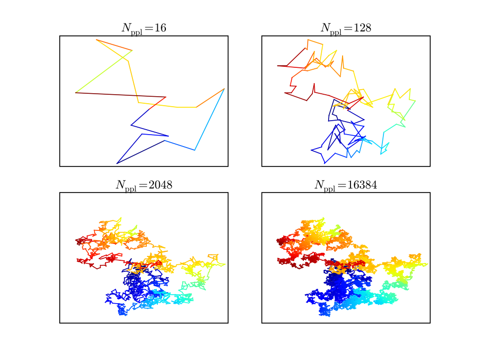
The above d-loop algorithm was selected since it is simple and about 10% faster than previous algorithms, according to its developers, because it requires fewer algebraic operations. The generation of the loops is largely independent from the main program. Because of this, it was simpler to generate the loops using a Matlab script. This function was used to produce text files containing the worldline data for ensembles of loops. These text files were read into memory at the launch of each calculation. The results of this generation routine can be seen in figure 1.

When the CUDA kernel is called, every thread in every block executes the kernel function with its own unique identifier. Therefore, it is best to generate worldlines in integer multiples of the number of threads per block.

Refer to caption — Figure 1: A single discrete worldline loop shown at several levels of discretization. The loops form fractal patterns and have a strong parallel with Brownian motion. The colour represents the phase of a particle travelling along the loop, and begins at dark blue, progresses in a random walk through yellow, and ends at dark red. The total flux through this particular worldline at $T=1$ and $B=B_{k}$ is about $0.08\pi/e$ .

II.2 Cylindrical Worldline Numerics

We now consider cylindrically symmetric external magnetic fields. In this case, we may simplify (6),

	$\displaystyle\frac{\Gamma^{(1)}_{\mathrm{ferm}}}{TL_{z}}$	$\displaystyle=$	$\displaystyle\frac{1}{4\pi}\int_{0}^{\infty}\rho_{\mathrm{cm}}\biggr[\int_{0}^{\infty}\frac{dT}{T^{3}}e^{-m^{2}T}\times$		(12)
			$\displaystyle~~~~~~\left\{\langle W\rangle_{{\bf r}_{\mathrm{cm}}}-1-\frac{1}{3}(eB_{\mathrm{cm}}T)^{2}\right\}\biggr]d\rho.$		(12)

II.2.1 Cylindrical Magnetic Fields

We have ${\bf B}=B(\rho)$ ${\bf\hat{z}}$ with

B(\rho)=\frac{A_{\phi}(\rho)}{\rho}+\frac{dA_{\phi}(\rho)}{d\rho}

(13)

if we make the gauge choice that $A_{0}=A_{\rho}=A_{z}=0$ .

We begin by considering $A_{\phi}(\rho)$ in the form

A_{\phi}(\rho)=\frac{F}{2\pi\rho}f_{\lambda}(\rho)

(14)

so that

B_{z}(\rho)=\frac{F}{2\pi\rho}\frac{df_{\lambda}(\rho)}{d\rho}

(15)

and the total flux is

\Phi=F(f_{\lambda}(L_{\rho})-f_{\lambda}(0)).

(16)

It is convenient to express the flux in units of $\frac{2\pi}{e}$ and define a dimensionless quantity

\mathcal{F}=\frac{e}{2\pi}F.

(17)

II.2.2 Wilson Loop

The quantity inside the angled brackets in equation (6) is a gauge invariant observable called a Wilson loop. We note that the proper time integral provides a natural path ordering for this operator. The Wilson loop expectation value is

\langle W\rangle_{{\bf r}_{\mathrm{cm}}}\!\!=\biggl\langle e^{ie\int_{0}^{T}d\tau{\bf A}({\bf r}_{\mathrm{cm}}+{\bf r}(\tau))\cdot\dot{{\bf r}}}\frac{1}{4}\mathrm{tr}e^{\frac{e}{2}\int_{0}^{T}d\tau\sigma_{\mu\nu}F_{\mu\nu}({\bf r}_{\mathrm{cm}}+{\bf r}(\tau))}\biggr\rangle_{{\bf r}_{\mathrm{cm}}}\!\!\!\!\!\!\!\!,

(18)

which we look at as a product between a scalar part ( $e^{ie\int_{0}^{T}d\tau{\bf A}({\bf r}_{\mathrm{cm}}+{\bf r}(\tau))\cdot\dot{{\bf r}}}$ ) and a fermionic part ( $\frac{1}{4}\mathrm{tr}e^{\frac{e}{2}\int_{0}^{T}d\tau\sigma_{\mu\nu}F_{\mu\nu}({\bf r}_{\mathrm{cm}}+{\bf r}(\tau))}$ ).

II.2.3 Scalar Part

In a magnetic field, the scalar part is related to the flux through the loop, $\Phi_{B}$ , by Stokes theorem:

	$\displaystyle e^{ie\int_{0}^{T}d\tau{\bf A}\cdot\dot{{\bf r}}}$	$\displaystyle=$	$\displaystyle e^{ie\oint{\bf A}\cdot d{\bf r}}=e^{ie\int_{{\bf\Sigma}}{\bf\nabla}\times{\bf A}\cdot d{\bf\Sigma}}$		(19)
		$\displaystyle=$	$\displaystyle e^{ie\int_{{\bf\Sigma}}{\bf B}d{\bf\Sigma}}=e^{ie\Phi_{B}}.$		(20)

Consequently, this factor accounts for the Aharonov-Bohm phase acquired by particles in the loop.

The loop discretization results in the following approximation of the scalar integral:

\oint{\bf A}({\bf r})\cdot d{\bf r}=\sum_{i=1}^{N_{\mathrm{ppl}}}\int_{{\bf r}^{i}}^{{\bf r}^{i+1}}{\bf A}({\bf r})\cdot d{\bf r}.

(21)

Using a linear parameterization of the positions, the line integrals are

\int_{{\bf r}^{i}}^{{\bf r}^{i+1}}{\bf A}({\bf r})\cdot d{\bf r}=\int_{0}^{1}dt{\bf A}({\bf r}(t))\cdot({\bf r}^{i+1}-{\bf r}^{i}).

(22)

Using the same gauge choice outlined above ( ${\bf A}=A_{\phi}\hat{\phi}$ ), we may write

{\bf A}({\bf r}(t))=\frac{\mathcal{F}}{e\rho^{2}}f_{\lambda}(\rho^{2})(-y,x,0),

(23)

where we have chosen $f_{\lambda}(\rho^{2})$ to depend on $\rho^{2}$ instead of $\rho$ to simplify some expressions and to avoid taking many costly square roots in the worldline numerics. We then have

\int_{{\bf r}^{i}}^{{\bf r}^{i+1}}{\bf A}({\bf r})\cdot d{\bf r}=\mathcal{F}(x^{i}y^{i+1}-y^{i}x^{i+1})\int_{0}^{1}dt\frac{f_{\lambda}(\rho_{i}^{2}(t))}{\rho_{i}^{2}(t)}.

(24)

The linear interpolation in Cartesian coordinates gives

\rho_{i}^{2}(t)=A_{i}+2B_{i}t+C_{i}t^{2},

(25)

where

$\displaystyle A_{i}$	$\displaystyle=$	$\displaystyle(x^{i})^{2}+(y^{i})^{2}$	(26)
$\displaystyle B_{i}$	$\displaystyle=$	$\displaystyle x^{i}(x^{i+1}-x^{i})+y^{i}(y^{i+1}-y^{i})$	(27)
$\displaystyle C_{i}$	$\displaystyle=$	$\displaystyle(x^{i+1}-x^{i})^{2}+(y^{i+1}-y^{i})^{2}.$	(28)

In performing the integrals along the straight lines connecting each discretized loop point, we are in danger of violating gauge invariance. If these integrals can be performed analytically, than gauge invariance is preserved exactly. However, in general, we wish to compute these integrals numerically. In this case, gauge invariance is no longer guaranteed, but can be preserved to any numerical precision that’s desired.

II.2.4 Fermion Part

For fermions, the Wilson loop is modified by a factor,

$\displaystyle W^{\mathrm{ferm.}}$	$\displaystyle=$	$\displaystyle\frac{1}{4}\mathrm{tr}\left(e^{\frac{1}{2}e\int_{0}^{T}d\tau\sigma_{\mu\nu}F^{\mu\nu}}\right)$	(29)
	$\displaystyle=$	$\displaystyle\frac{1}{4}\mathrm{tr}\left(e^{\sigma_{xy}e\int_{0}^{T}d\tau B\left(x(\tau)\right)}\right)$	(30)
	$\displaystyle=$	$\displaystyle\cosh{\left(e\int_{0}^{T}d\tau B\left(x(\tau)\right)\right)}$	(31)
	$\displaystyle=$	$\displaystyle\cosh{\left(2\mathcal{F}\int_{0}^{T}d\tau f^{\prime}_{\lambda}(\rho^{2}(\tau))\right)},$	(32)

where we have used the relation

eB=2\mathcal{F}\frac{df_{\lambda}(\rho^{2})}{d\rho^{2}}=2\mathcal{F}f^{\prime}_{\lambda}(\rho^{2}).

(33)

This factor represents an additional contribution to the action because of the spin interaction with the magnetic field. Classically, for a particle with a magnetic moment ${\bf\mu}$ travelling through a magnetic field in a time $T$ , the action is modified by a term given by

\Gamma^{0}_{\mathrm{spin}}=\int_{0}^{T}{\bf\mu}\cdot{\bf B}({\bf x}(\tau))d\tau.

(34)

The magnetic moment is related to the electron spin ${\bf\mu}=g\left(\frac{e}{2m}\right){\bf\sigma}$ , so we see that the integral in the above quantum fermion factor is very closely related to the classical action associated with transporting a magnetic moment through a magnetic field:

\Gamma^{0}_{\mathrm{spin}}=g\left(\frac{e}{2m}\right)\sigma_{xy}\int_{0}^{T}B_{z}(x(\tau))d\tau.

(35)

Qualitatively, we could write

W^{\mathrm{ferm}}\sim\cosh{\left(\Gamma^{0}_{\mathrm{spin}}\right)}.

(36)

As a possibly useful aside, we may want to express the integral in terms of $f_{\lambda}(\rho^{2})$ instead of its derivative. We can do this by integrating by parts:

$\displaystyle\int_{0}^{T}d\tau f^{\prime}_{\lambda}(\rho^{2}(\tau))$	$\displaystyle=$	$\displaystyle\frac{T}{N_{\mathrm{ppl}}}\sum_{i=1}^{N_{\mathrm{ppl}}}\int_{0}^{1}dtf^{\prime}_{\lambda}(\rho^{2}_{i}(\tau))$	(38)
	$\displaystyle=$	$\displaystyle\frac{T}{N_{\mathrm{ppl}}}\sum_{i=1}^{N_{\mathrm{ppl}}}\biggr[\frac{f_{\lambda}(\rho^{2}_{i}(t))}{2(B_{i}+C_{i}t)}\biggr\|^{t=1}_{t=0}$
		$\displaystyle+\frac{C_{i}}{2}\!\!\int_{0}^{1}\!\!\!\!\frac{f_{\lambda}(\rho^{2}_{i}(t))}{(B_{i}+C_{i}t)^{2}}dt\biggr]$
	$\displaystyle=$	$\displaystyle\frac{T}{N_{\mathrm{ppl}}}\sum_{i=1}^{N_{\mathrm{ppl}}}\frac{C_{i}}{2}\!\!\int_{0}^{1}\!\!\!\!\frac{f_{\lambda}(\rho^{2}_{i}(t))}{(B_{i}+C_{i}t)^{2}}dt,$	(39)

with $\rho_{i}^{2}(t)$ given by equations (25) to (28). The second equality is obtained from integration-by-parts. In the third equality, we use the loop sum to cancel the boundary terms in pairs:

W^{\mathrm{ferm.}}=\cosh{\left(\frac{\mathcal{F}T}{N_{\mathrm{ppl}}}\sum_{i=1}^{N_{\mathrm{ppl}}}C_{i}\int_{0}^{1}dt\frac{f_{\lambda}(\rho^{2}_{i}(t))}{(B_{i}+C_{i}t)^{2}}\right)}.

(40)

In most cases, one would use equation (32) to compute the fermion factor of the Wilson loop. However, equation (40) may be useful in cases where $f^{\prime}_{\lambda}(\rho^{2}(\tau))$ is not known or is difficult to compute.

II.2.5 Renormalization

The field strength renormalization counterterms result from the small $T$ behaviour of the worldline integrand. In the limit where $T$ is very small, the worldline loops are very localized around their center of mass. So, we may approximate their contribution as being that of a constant field with value ${\bf A}({\bf r}_{\mathrm{cm}})$ . Specifically, we require that the field change slowly on the length scale defined by $\sqrt{T}$ . This condition on $T$ can be written

T\ll\left|\frac{m^{2}}{eB^{\prime}(\rho^{2})}\right|=\left|\frac{m^{2}}{2\mathcal{F}f^{\prime\prime}_{\lambda}(\rho^{2}_{\mathrm{cm}})}\right|.

(41)

When this limit is satisfied, we may use the exact expressions for the constant field Wilson loops to determine the small $T$ behaviour of the integrands and the corresponding counterterms.

The Wilson loop averages for constant magnetic fields in scalar and fermionic QED are

\langle W\rangle_{\mathrm{ferm}}=eBT\coth{(eBT)}

(42)

and

\langle W\rangle_{\mathrm{scal}}=\frac{eBT}{\sinh{(eBT)}}.

(43)

Therefore, the integrand for fermionic QED in the limit of small $T$ is

	$\displaystyle I_{\mathrm{ferm}}(T)$	$\displaystyle=$	$\displaystyle\frac{e^{-m^{2}T}}{T^{3}}\left[eB({\bf r}_{cm})T\coth{(eB({\bf r}_{cm})T)}-1-\frac{e^{2}}{3}B^{2}({\bf r}_{cm})T^{2}\right]$		(44)
		$\displaystyle\approx$	$\displaystyle-\frac{(eB)^{4}T}{45}+\frac{1}{45}(eB)^{4}m^{2}T^{2}+\left(\frac{2(eB)^{6}}{945}-\frac{(eB)^{4}m^{4}}{90}\right)T^{3}+\frac{(7(eB)^{4}m^{6}-4(eB)^{6}m^{2})T^{4}}{1890}+O(T^{5}).$		(44)

For scalar QED we have

	$\displaystyle I_{\mathrm{scal}}(T)$	$\displaystyle=$	$\displaystyle\frac{e^{-m^{2}T}}{T^{3}}\left[\frac{eB({\bf r}_{cm})T}{\sinh{(eB({\bf r}_{cm})T)}}-1+\frac{1}{6}(eB)^{2}({\bf r}_{cm})T^{2}\right]$		(45)
		$\displaystyle\approx$	$\displaystyle\frac{7(eB)^{4}T}{360}-\frac{7(eB)^{4}m^{2}T^{2}}{360}+\frac{(147(eB)^{4}m^{4}-31(eB)^{6})T^{3}}{15120}+\frac{(31(eB)^{6}m^{2}-49(eB)^{4}m^{6})T^{4}}{15120}+O(T^{5}).$		(45)

Beyond providing the renormalization conditions, these expansions can be used in the small $T$ regime to avoid a problem with the Wilson loop uncertainties in this region. Consider the uncertainty in the integrand arising from the uncertainty in the Wilson loop:

\delta I(T)=\frac{\partial I}{\partial W}\delta W=\frac{e^{-m^{2}T}}{T^{3}}\delta W.

(46)

In this case, even though we can compute the Wilson loops for small $T$ precisely, even a small uncertainty is magnified by a divergent factor when computing the integrand for small values of $T$ . So, in order to perform the integral, we must replace the small $T$ behaviour of the integrand with the above expansions (44) and (45). Our worldline integral then proceeds by analytically computing the integral for the small $T$ expansion up to some small value, $a$ , and adding this to the remaining part of the integral [26]:

\int_{0}^{\infty}I(T)dT=\underbrace{\int_{0}^{a}I(T)dT}_{\mathrm{small~T}}+\underbrace{\int_{a}^{\infty}I(T)dT}_{\mathrm{worldline~numerics}}.

(47)

Because this normalization procedure uses the constant field expressions for small values of $T$ , this scheme introduces a small systematic uncertainty. To improve on the method outlined here, the derivatives of the background field can be accounted for by using the analytic forms of the heat kernel expansion to perform the renormalization [2].

II.3 Uncertainty analysis in worldline numerics

So far in the worldline numerics literature, the discussions of uncertainty analysis have been unfortunately brief. It has been suggested that the standard deviation of the worldlines provides a good measure of the statistical error in the worldline method [1, 2]. However, the distributions produced by the worldline ensemble are highly non-Gaussian (see figure 5), and therefore the standard error in the mean is not a good measure of the uncertainties involved. Furthermore, the use of the same worldline ensemble to compute the Wilson loop multiple times in an integral results in strongly correlated uncertainties. Thus, propagating uncertainties through integrals can be computationally expensive due to the complexity of computing correlation coefficients.

The error bars on worldline calculations impact the conclusions that can be drawn from calculations, and also have important implications for the fermion problem, which limits the domain of applicability of the technique (see section II.3.6). It is therefore important that the error analysis is done thoughtfully and transparently. The purpose of this section is to contribute a more thorough discussion of uncertainty analysis in the worldline numerics technique to the literature in hopes of avoiding any confusion associated with the above-mentioned subtleties.

There are two sources of uncertainty in the worldline technique: the discretization error in treating each continuous worldline as a set of discrete points, and the statistical error of sampling a finite number of possible worldlines from a distribution. In this section, we discuss each of these sources of uncertainty.

II.3.1 Estimating the Discretization Uncertainties

The discretization error arising from the integral over $\tau$ in the exponent of each Wilson loop (see equation (18)) is difficult to estimate since any number of loops could be represented by each choice of discrete points. The general strategy is to make this estimation by computing the Wilson loop using several different numbers of points per worldline and observing the convergence properties.

The specific procedure adopted for this work involves dividing each discrete worldline into several worldlines with varying levels of discretization. Since we are using the d-loop method for generating the worldlines (section II.1.1), a $\frac{N_{\mathrm{ppl}}}{2}$ sub-loop consisting of every other point will be guaranteed to contain the prescribed distribution of velocities.

To look at the convergence for the loop discretization, each worldline is divided into three groups. One group of $\frac{N_{\mathrm{ppl}}}{2}$ points, and two groups of $\frac{N_{\mathrm{ppl}}}{4}$ . This permits us to compute the average holonomy factors at three levels of discretization:

\langle W\rangle_{N_{\mathrm{ppl}}/4}=\langle e^{\frac{i}{2}\triangle}e^{\frac{i}{2}\Box}\rangle,

(48)

\langle W\rangle_{N_{\mathrm{ppl}}/2}=\langle e^{i\circ}\rangle,

(49)

and

\langle W\rangle_{N_{\mathrm{ppl}}}=\langle e^{\frac{i}{2}\circ}e^{\frac{i}{4}\Box}e^{\frac{i}{4}\triangle}\rangle,

(50)

where the symbols $\circ$ , $\Box$ , and $\triangle$ denote the worldline integral, $\int_{0}^{T}d\tau A(x_{CM}+x(\tau))\cdot\dot{x}$ , computed using the sub-worldlines depicted in figure 2.

We may put these factors into the equation of a parabola to extrapolate the result to an infinite number of points per line (see figure 3):

\langle W\rangle_{\infty}\approx\frac{8}{3}\langle W\rangle_{N_{\mathrm{ppl}}}-2\langle W\rangle_{N_{\mathrm{ppl}}/2}+\frac{1}{3}\langle W\rangle_{N_{\mathrm{ppl}}/4}.

(51)

So, we estimate the discretization uncertainty to be

\delta\langle W\rangle_{\infty}\approx|\langle W\rangle_{N_{\mathrm{ppl}}}-\langle W\rangle_{\infty}|.

(52)

Generally, the statistical uncertainties are the limitation in the precision of the worldline numerics technique. Therefore, $N_{\mathrm{ppl}}$ should be chosen to be large enough that the discretization uncertainties are small relative to the statistical uncertainties.

II.3.2 Estimating the Statistical Uncertainties

We can gain a great deal of insight into the nature of the statistical uncertainties by examining the specific case of the uniform magnetic field since we know the exact solution in this case. Sections II.3.3, II.3.4, and II.3.5 discuss the peculiarities of the statisical uncertainties in the worldline numerics method for the uniform magnetic field.

II.3.3 The Worldline Ensemble Distribution is not Normal

A reasonable first instinct for estimating the error bars is to use the standard error in the mean of the collection of individual worldlines:

\mathrm{SEM}(W)=\sqrt{\sum_{i=1}^{N_{l}}\frac{(W_{i}-\langle W\rangle)^{2}}{N_{l}(N_{l}-1)}}.

(53)

This approach has been promoted in early papers on worldline numerics [1, 2]. In figure 4, we have plotted the residuals and the corresponding error bars for several values of the proper time parameter, $T$ in black. From this plot, it appears that the error bars are quite large in the sense that we appear to produce residuals which are considerably smaller than would be implied by the sizes of the error bars. This suggests that we have overestimated the size of the uncertainty.

Figure 4: The residuals of the Wilson loops for a constant magnetic field showing the standard error in the mean (thin error bars) and the uncertainty in determining the mean (thick blue error bars). For reasons discussed in this section, the standard error in the mean overestimates the uncertainties involved by more than a factor of 3 at each value of

T

We can see why this is the case by looking more closely at the distributions produced by the worldline technique. An exact expression for these distributions can be derived in the case of the constant magnetic field [26]:

	$\displaystyle w(y)$	$\displaystyle=$	$\displaystyle\frac{W_{\mathrm{exact}}}{\sqrt{1-y^{2}}}\sum_{n=-\infty}^{\infty}\biggl[f(\arccos(y)+2n\pi)+$		(54)
			$\displaystyle~~~~~~~~~~~~f(-\arccos(y)+2n\pi)\biggr]$		(54)

with

f(\phi)=\frac{\pi}{4BT\cosh^{2}(\frac{\pi\phi}{2BT})}.

(55)

Figure 5 shows histograms of the worldline results along with the expected distributions. These distributions highlight a significant hurdle in assigning error bars to the results of worldline numerics.

Figure 5: Histograms showing the worldline distributions of the residuals for three values of

T

in the constant magnetic field case. Here, we are neglecting the fermion factor. The dark line represents the exact distribution computed using equation 54. The worldline means are indicated with an arrow, while the exact mean in each case is 0. There are 5120 worldlines in each histogram. The vertical axes are normalized to a total area of unity.

Due to their highly non-Gaussian nature, the standard error in the mean is not a good characterization of the distributions that are produced. We should not interpret each individual worldline as an independent measurement of the mean value of these distributions; for large values of $BT$ , almost all of our worldlines will produce answers which are far away from the mean of the distribution. This means that the variance of the distribution will be very large, even though our ability to determine the mean of the distribution is relatively precise because of the increasing symmetry about the mean as $T$ becomes large.

II.3.4 Correlations between Wilson Loops

Typically, numerical integration is performed by replacing the integral with a sum over a finite set of points from the integrand. We will begin the present discussion by considering the uncertainty in adding together two points (labelled $i$ and $j$ ) in our integral over $T$ . Two terms of the sum representing the numerical integral will involve a function of $T$ times the two Wilson loop factors,

I=g(T_{i})\langle W(T_{i})\rangle+g(T_{j})\langle W(T_{j})\rangle

(56)

with an uncertainty given by

$\displaystyle\delta I$	$\displaystyle=$	$\displaystyle\left\|\frac{\partial I}{\partial\langle W(T_{i})\rangle}\right\|^{2}(\delta\langle W(T_{i})\rangle)^{2}$	(58)
		$\displaystyle~~+\left\|\frac{\partial I}{\partial\langle W(T_{j})\rangle}\right\|^{2}(\delta\langle W(T_{j})\rangle)^{2}$
		$\displaystyle~~+2\left\|\frac{\partial I}{\partial\langle W(T_{i})\rangle}\frac{\partial I}{\partial\langle W(T_{j})\rangle}\right\|\times$
		$\displaystyle~~\rho_{ij}(\delta\langle W(T_{i})\rangle)(\delta\langle W(T_{j})\rangle)$
	$\displaystyle=$	$\displaystyle g(T_{i})^{2}(\delta\langle W(T_{i})\rangle)^{2}+g(T_{j})^{2}(\delta\langle W(T_{j})\rangle)^{2}+$
		$\displaystyle~2\left\|g(T_{i})g(T_{j})\right\|\rho_{ij}(\delta\langle W(T_{i})\rangle)(\delta\langle W(T_{j})\rangle)$

and the correlation coefficient $\rho_{ij}$ given by

\rho_{ij}=\frac{\langle(W(T_{i})-\langle W(T_{i})\rangle)(W(T_{j})-\langle W(T_{j})\rangle)\rangle}{\sqrt{(W(T_{i})-\langle W(T_{i})\rangle)^{2}}\sqrt{(W(T_{j})-\langle W(T_{j})\rangle)^{2}}}.

(59)

The final term in the error propagation equation takes into account correlations between the random variables $W(T_{i})$ and $W(T_{j})$ . Often in a Monte Carlo computation, one can treat each evaluation of the integrand as independent, and neglect the uncertainty term involving the correlation coefficient. However, in worldline numerics, the evaluations are related because the same worldline ensemble is reused for each evaluation of the integrand. The correlations are significant (see figure 6), and this term can’t be neglected. Computing each correlation coefficient takes a time proportional to the square of the number of worldlines. Therefore, it may be computationally expensive to formally propagate uncertainties through an integral.

Figure 6: Correlation coefficients, equation (59), between

\langle W(T)\rangle

and

\langle W(T=3)\rangle

computed using individual worldlines, groups of worldlines, and shuffled groups of worldlines.

The point-to-point correlations were originally pointed out by Gies and Langfeld who addressed the problem by updating (but not replacing or regenerating) the loop ensemble in between each evaluation of the Wilson loop average [1]. This may be a good way of addressing the problem. However, in the following section, we promote a method which can bypass the difficulties presented by the correlations by treating the worldlines as a collection of worldline groups.

II.3.5 Grouping Worldlines

Both of the problems explained in the previous two subsections can be overcome by creating groups of worldline loops within the ensemble. Each group of worldlines then makes a statistically independent measurement of the Wilson loop average for that group. The statistics between the groups of measurements are normally distributed, and so the uncertainty is the standard error in the mean of the ensemble of groups (in contrast to the ensemble of worldlines).

For example, if we divide the $N_{l}$ worldlines into $N_{G}$ groups of $N_{l}/N_{G}$ worldlines each, we can compute a mean for each group:

\langle W\rangle_{G_{j}}=\frac{N_{G}}{N_{l}}\sum_{i=1}^{N_{l}/N_{G}}W_{i}.

(60)

Provided each group contains the same number of worldlines, the average of the Wilson loop is unaffected by this grouping:

	$\displaystyle\langle W\rangle$	$\displaystyle=$	$\displaystyle\frac{1}{N_{G}}\sum_{j=1}^{N_{G}}\langle W\rangle_{G_{j}}$		(61)
		$\displaystyle=$	$\displaystyle\frac{1}{N_{l}}\sum_{i=1}^{N_{l}}W_{i}.$		(62)

However, the uncertainty is the standard error in the mean of the groups,

\delta\langle W\rangle=\sqrt{\sum_{i=1}^{N_{G}}\frac{(\langle W\rangle_{G_{i}}-\langle W\rangle)^{2}}{N_{G}(N_{G}-1)}}.

(63)

Because the worldlines are unrelated to one another, the choice of how to group them to compute a particular Wilson loop average is arbitrary. For example, the simplest choice is to group the loops by the order they were generated, so that a particular group number, $i$ , contains worldlines $iN_{l}/N_{G}$ through $(i+1)N_{l}/N_{G}-1$ . Of course, if the same worldline groupings are used to compute different Wilson loop averages, they will still be correlated. We will discuss this problem in a moment.

The basic claim of the worldline technique is that the mean of the worldline distribution approximates the holonomy factor. However, from the distributions in figure 5, we can see that the individual worldlines themselves do not approximate the holonomy factor. So, we should not think of an individual worldline as an estimator of the mean of the distribution. Thus, a resampling technique is required to determine the precision of our statistics. We can think of each group of worldlines as making an independent measurement of the mean of a distribution. As expected, the groups of worldlines produce a more Gaussian-like distribution (see figure 7), and so the standard error of the groups is a sensible measure of the uncertainty in the Wilson loop value.

Figure 7: The histogram demonstrating the precision with which we can reproduce measurements of the mean using different groups of 100 worldlines at

BT=6.0

. In this case, the distribution is Gaussian-like and meaningful error bars can be placed on our measurement of the mean.

We find that the error bars are about one-third as large as those determined from the standard error in the mean of the individual worldlines, and the smaller error bars better characterize the size of the residuals in the constant field case (see figure 4). The strategy of using subsets of the available data to determine error bars is called jackknifing. Several previous papers on worldline numerics have mentioned using jackknife analysis to determine the uncertainties, but without an explanation of the motivations or the procedure employed [10, 9, 6, 11].

The grouping of worldlines alone does not address the problem of correlations between different evaluations of the integrands. Figure 6 shows that the uncertainties for groups of worldlines are also correlated between different points of the integrand. However, the worldline grouping does provide a tool for bypassing the problem. One possible strategy is to randomize how worldlines are assigned to groups between each evaluation of the integrand. This produces a considerable reduction in the correlations, as is shown in figure 6. Then, errors can be propagated through the integrals by neglecting the correlation terms. Another strategy is to separately compute the integrals for each group of worldlines, and then consider the statistics of the final product to determine the error bars. This second strategy is the one adopted for the work presented in this paper. Grouping in this way reduces the amount of data which must be propagated through the integrals by a factor of the group size compared to a delete-1 jackknife scheme, for example. In general, the error bars quoted in the remainder of this paper are obtained by computing the standard error in the mean of groups of worldlines.

II.3.6 Uncertainties and the Fermion Problem

The fermion problem of worldline numerics is a name given to an enhancement of the uncertainties at large $T$ [1, 26]. It should not be confused with the fermion-doubling problem associated with lattice methods. In a constant magnetic field, the scalar portion of the calculation produces a factor of $\frac{BT}{\sinh{(BT)}}$ , while the fermion portion of the calculation produces an additional factor $\cosh{(BT)}$ . Physically, this contribution arises as a result of the energy required to transport the electron’s magnetic moment around the worldline loop. At large values of $T$ , we require subtle cancellation between huge values produced by the fermion portion with tiny values produced by the scalar portion. However, for large $T$ , the scalar portion acquires large relative uncertainties which make the computation of large $T$ contributions to the integral very imprecise.

This can be easily understood by examining the worldline distributions shown in figure 5. Recall that the scalar Wilson loop average for these histograms is given by the flux in the loop, $\Phi_{B}$ :

\langle W\rangle=\left<\exp{\left(ie\int_{0}^{T}d\tau{\bf A}({\bf x}_{\mathrm{cm}}+{\bf x}(\tau))\cdot d{\bf x}(\tau)\right)}\right>=\left<e^{ie\Phi_{B}}\right>.

(64)

For constant fields, the flux through the worldline loops obeys the distribution function [26]

f(\Phi_{B})=\frac{\pi}{4BT\cosh^{2}\left(\frac{\pi\Phi_{B}}{2BT}\right)}.

(65)

For small values of $T$ , the worldline loops are small and the amount of flux through the loop is correspondingly small. Therefore, the flux for small loops is narrowly distributed about $\Phi_{B}=0$ . Since zero maximizes the Wilson loop ( $e^{i0}=1$ ), this explains the enhancement to the right of the distribution for small values of $T$ . As $T$ is increased, the flux through any given worldline becomes very large and the distribution of the flux becomes very broad. For very large $T$ , the width of the distribution is many factors of $2\pi/e$ . Then, the phase ( $e\Phi_{B}\mod{2\pi}$ ) is nearly uniformly distributed, and the Wilson loop distribution reproduces the Chebyshev distribution (i.e. the distribution obtained from projecting uniformly distributed points on the unit circle onto the horizontal axis),

\lim_{T\to\infty}w(y)=\frac{1}{\pi\sqrt{1-y^{2}}}.

(66)

The mean of the Chebyshev distribution is zero due to its symmetry. However, this symmetry is not realized precisely unless we use a very large number of loops. Since the width of the distribution is already 100 $\times$ the value of the mean at $T=6$ , any numerical asymmetries in the distribution result in very large relative uncertainties of the scalar portion. Because of these uncertainties, the large contribution from the fermion factor are not cancelled precisely.

This problem makes it very difficult to compute the fermionic effective action unless the fields are well localized [26]. For example, the fermionic factor for non-homogeneous magnetic fields oriented along the z-direction is

\cosh{\left(e\int_{0}^{T}d\tau B(x(\tau))\right)}.

(67)

For a homogeneous field, this function grows exponentially with $T$ and is cancelled by the exponentially vanishing scalar Wilson loop. For a localized field, the worldline loops are very large for large values of $T$ , and they primarily explore regions far from the field. Thus, the fermionic factor grows more slowly in localized fields, and is more easily cancelled by the rapidly vanishing scalar part.

Figure 8: The small

T

behaviour of worldline numerics. The data points represent the numerical results, where the error bars are determined from the jackknife analysis described in chapter II.3. The solid line represents the exact solution while the dotted line represents the small

T

expansion of the exact solution. Note the amplification of the uncertainties.

II.4 Computing an Effective Action

The ensemble average in the effective action is simply the sum over the contributions from each worldline loop, divided by the number of loops in the ensemble. Since the computation of each loop is independent of the other loops, the ensemble average may be straightforwardly parallelized by generating separate processes to compute the contribution from each loop. For this parallelization, four Nvidia Tesla C1060 GPU were used through the CUDA parallel programming framework. Because GPU can spawn thousands of parallel processing threads with much less computational overhead than an MPI cluster, they excel at handling a very large number of parallel threads, although the clock speed is slower and fewer memory resources are typically available. The GPU architecture has recently been used by another group for computing Casimir forces using worldline numerics [27]. More detailed information about the technical implementation of these calculations on the GPU architecture, including a listing of the source code, can be found in [28].

Once the ensemble average of the Wilson loop has been computed, computing the effective action is a straightforward matter of performing numerical integrals. The effective action density is computed by performing the integration over proper time, $T$ . Then, the effective action is computed by performing a spacetime integral over the loop ensemble center of mass. In all cases where a numerical integral was performed, Simpson’s method was used [29]. Integrals from 0 to $\infty$ were mapped to the interval $[0,1]$ using substitutions of the form $x=\frac{1}{1+T/T_{\mathrm{max}}}$ , where $T_{\mathrm{max}}$ sets the scale for the peak of the integrand. In the constant field case, for the integral over proper time, we expect $T_{\mathrm{max}}\sim 3/(eB)$ for large fields and $T_{\mathrm{max}}\sim 1$ for fields of a few times critical or smaller. In section II.3, we presented a detailed discussion of how the statistical and discretization uncertainties can be computed in this technique.

II.5 Verification and Validation

The worldline numerics software can be validated and verified by making sure that it produces the correct results where the derivative expansion is a good approximation, and that the results are consistent with previous numerical calculations of flux tube effective actions. For this reason, the validation was done primarily with flux tubes with a profile defined by the function

f_{\lambda}(\rho^{2})=\frac{\rho^{2}}{(\lambda^{2}+\rho^{2})}.

(68)

For large values of $\lambda$ , this function varies slowly on the Compton wavelength scale, and so the derivative expansion is a good approximation. Also, flux tubes with this profile were studied previously using worldline numerics [7, 26].

Among the results presented in [26] is a comparison of the derivative expansion and worldline numerics for this magnetic field configuration. The result is that the next-to-leading-order term in the derivative expansion is only a small correction to the the leading-order term for $\lambda\gg\lambda_{e}$ , where the derivative expansion is a good approximation. The derivative expansion breaks down before it reaches its formal validity limits at $\lambda\sim\lambda_{e}$ . For this reason, we will simply focus on the leading order derivative expansion, which we call the locally-constant-field (LCF) approximation. The effective action of QED in the LCF approximation is given in cylindrical symmetry by

$\displaystyle\Gamma^{(1)}_{\mathrm{ferm}}$	$\displaystyle=$	$\displaystyle\frac{1}{4\pi}\int_{0}^{\infty}dT\int_{0}^{\infty}\rho_{\mathrm{cm}}d\rho_{\mathrm{cm}}\frac{e^{-m^{2}T}}{T^{3}}\times$	(69)
		$\displaystyle\biggl\{eB(\rho_{\mathrm{cm}})T\coth{(eB(\rho_{\mathrm{cm}})T)}$
		$\displaystyle-1-\frac{1}{3}(eB(\rho_{\mathrm{cm}})T)^{2}\biggr\}.$

Figure 9: The integrand of the proper time,

T

, integral for three different values of the radial coordinate,

\rho

for a

\lambda=1

flux tube. The solid lines represent the zeroth-order derivative expansion, which, as expected, is a good approximation until

\rho

becomes too small.

Figure 9 shows a comparison between the proper time integrand,

\frac{e^{-m^{2}T}}{T^{3}}\left[\langle W\rangle_{{\bf r}_{\mathrm{cm}}}-1-\frac{1}{3}(eB_{\mathrm{cm}}T)^{2}\right],

(70)

and the LCF approximation result for a flux tube with $\lambda=\lambda_{e}$ and $\mathcal{F}=10$ . In this case, the LCF approximation is only appropriate far from the center of the flux tube, where the field is not changing very rapidly. In the figure, we can begin to see the deviation from this approximation, which gets more pronounced closer to the center of the flux tube (smaller values of $\rho$ ).

Figure 10: The fermion term of the effective action density as a function of the radial coordinate for a flux tube with width

\lambda=10\lambda_{e}

The effective action density for a slowly varying flux tube is plotted in figure 10 along with the LCF approximation. In this case, the LCF approximation agrees within the statistics of the worldline numerics.

III Astrophysical Background

III.1 Nuclear Superconductivity in Neutron Stars

In the dense nuclear matter of a neutron star, it may be possible to have neutron superfluidity, proton superconductivity, and even quark colour superconductivity [13, 14]. The first prediction of neutron-star superfluidity dates back to Migdal in 1959 [30]. The arguments which make superfluidity seem likely are based on the temperatures of neutron stars. A short time after their creation, neutron stars are very cold compared to nuclear energy scales. The temperature in the interior may be a few hundred keV. Studies of nuclear matter show that the transition temperature is $T_{c}\gtrsim 500$ keV [31]. So, it is expected that the nuclear matter in a neutron star forms condensates of Cooper pairs.

Because of this, some fraction of neutrons in the inner crust of a neutron star are expected to be superfluid. These neutrons make up about a percent of the moment of inertia of the star and are weakly coupled to the nuclear crystal lattice which makes up the remainder of the inner crust. If the neutron vortices in the superfluid component move at nearly the same speed as the nuclear lattice, the vortices can become pinned to the lattice so that the superfluid shares an angular velocity with the crust. This pinning between the fluid and solid crust has observable impacts on the rotational dynamics of the neutron star, for the same reasons that hard-boiling an egg (pinning the yolk to the shell) produces an observable difference in the way it spins.

This picture of a neutron superfluid co-rotating with a solid crust has been used to interpret several types of pulsar timing anomalies. Pulsars are nearly perfect clocks, although they gradually spin-down as they radiate energy. Occasionally, though, pulsars demonstrate deviations from their expected regularity. A glitch is an abrupt increase in the rotation and spin-down rate of a pulsar, followed by a slow relaxation to pre-glitch values over weeks or years. This behaviour is consistent with the neutron superfluid suddenly becoming unpinned from the crust and then dynamically relaxing due to its weak coupling to the crust until it is pinned once again [32].

The neutron star in Cassiopeia A has been observed to be rapidly cooling [33]. The surface temperature has decreased by about 4% over 10 years. This observation is also strong evidence of superfluidity and superconductivity in neutron stars [34, 35]. The observed cooling is too fast to be explained by the observed x-ray emissions and standard neutrino cooling. However, the cooling is readily explained by the emission of neutrinos during the formation of neutron Cooper pairs. Based on such a model, the superfluid transition temperature of neutron star matter is $\sim 10^{9}$ K or $\sim 90$ keV.

Further hints regarding superfluidity in neutron stars come from long-term periodic variability in pulsar timing data. For example, variabilities in PSR B1828-11 were initially interpreted as free precession (or wobble) of the star [36]. If neutron stars can precess, observations could strongly constrain the ratio of the moments of inertia of the crust and the superfluid neutrons. Moreover, the existence of flux tubes (i.e. type-II superconductivity) in the crust is generally incompatible with the slow, large amplitude precession suggested by PSR B1828-11 [36]. The neutron vortices would have to pass through the flux tubes, which should cause a huge dissipation of energy and a dampening of the precession which is not observed [37]. However, recent arguments suggest that the timing variability data is not well explained by free precession and that it more likely suggests that the star is switching between two magnetospheric states [38]. Nevertheless, other authors suggest not being premature in throwing out the precession hypothesis without further observations [39].

III.2 Magnetic Flux Tubes in Neutron Stars

If a magnetic field is able to penetrate the proton superfluid on a microscopic level, it must do so by forming a triangular Abrikosov lattice with a single quanta of flux in each flux tube. So, the density of flux tubes is given simply by the average field strength. If the distance between flux tubes is $l_{f}$ , the flux in a circular region within $l_{f}/2$ of a flux tube is given by

F=\frac{2\pi\mathcal{F}}{e}=2\pi\int_{0}^{l_{f}/2}B\rho d\rho

(71)

where we have introduced a dimensionless measure of flux $\mathcal{F}=\frac{e}{2\pi}F$ . So, the distance between flux tubes is

l_{f}=\sqrt{\frac{8\mathcal{F}}{eB}}.

(72)

If the magnetic field is the quantum critical field strength, $B_{k}=\frac{m^{2}}{e}=4.4\times 10^{13}$ Gauss, then the flux tubes are separated by a few Compton electron wavelengths. This is particularly interesting since this is the distance scale associated with non-locality in QED.

The size of a flux tube profile in laboratory superconductors is on the nanometer or micron scale [40]. Because the flux is fixed, the size of the tube profile determines the strength of the magnetic field within the tube. For laboratory superconductors the field strengths are small compared to the quantum critical field, and the field is slowly varying on the scale of the Compton wavelength. In this case, the quantum corrections to the free energy are known to be much smaller than the classical contribution (see section III.3). The size scale for the flux tubes in a superconductor is determined by the London penetration depth. In a neutron star, this quantity is estimated to be a small fraction of a Compton wavelength, much smaller than in laboratory superconductors [41, 37]. In this case, the magnetic field strength at the centre of the tube exceeds the quantum critical field strength and the field varies rapidly, rendering the derivative expansion description of the effective action unreliable.

The Ginzburg-Landau parameter, equation is the ratio of the proton coherence length, $\xi_{p}\sim 30$ fm, and the London penetration depth of a proton superconductor, $\lambda_{p}\sim 80$ fm [37].

\kappa=\frac{\lambda_{p}}{\xi_{p}}\sim 2

(73)

where $\kappa>1/\sqrt{2}$ signals Type-II behavior. We therefore expect that the proton Cooper pairs most likely form a type-II superconductor [13]. However, it is possible that physics beyond what is taken into account in the standard picture affects the free energy of a magnetic flux tube. In that case, the interaction between two flux tubes may indeed be attractive in which case the neutron star would be a type-I superconductor.

III.3 QED Effective Actions of Flux Tubes

Vortices of magnetic flux have very important impacts on the quantum mechanics of electrons. In particular, the phase of the electron’s wavefunction is not unique in such a magnetic field. This is demonstrated by the Aharonov-Bohm effect [42, 43]. The first calculations of the fermion effective energies of these configurations were for infinitely thin Aharonov-Bohm flux strings [44, 45]. Calculations for thin strings were also performed for cosmic string configurations [46]. For these infinitely-thin string magnetic fields, the energy density is singular for small radii. So, it is not possible to define a total energy per unit length. Another approach was to compute the effective action for a finite-radius flux tube where the magnetic flux was confined entirely to the surface of the tube [47]. This approach results in infinite classical energy densities as well.

Physical flux tube configurations would have a finite radius. The earliest paper to deal with finite radius flux tubes in QED considered the effective action of a step-function profiled flux tube using the Jost function of the related scattering problem [48]. One of the conclusions from this research was that the quantum correction to the classical energy was relatively small for any value of the flux tube size, for the entire range of applicability of QED. The techniques from this study were soon generalized to other field profiles including, a delta-function cylindrical shell magnetic field [49], and more realistic flux tube configurations such as the Gaussian [50] and the Nielsen-Olesen vortex [51]. Flux tube vacuum energies were also analyzed extensively using a spectral method [52, 53, 54].

The effective actions of flux tubes have been previously analyzed using worldline numerics [3]. This research investigated isolated flux tubes, but also made use of the loop cloud method’s applicability to situations of low symmetry to investigate pairs of interacting vortices. One conclusion from that investigation was that the fermionic effects resulted in an attractive force between vortices with parallel orientations, and a repulsive force between vortices with anti-parallel orientations. Due to the similarity in scope and technique, the latter mentioned research is the closest to the research presented in this paper.

IV Calculations

In this section, we will further explore the nature of this phenomenon in QED using a highly parallel implementation of the worldline numerics technique implemented on a heterogeneous CPU and GPU architecture. Specifically, we explore cylindrically symmetric magnetic field profiles for isolated flux tubes and periodic profiles designed to model properties of a triangular lattice. For these calculations, the classical magnetic field configurations are a chosen input to the algorithms and the physical processes that may have created the field configurations do not factor in to the calculations. The worldline numerics algorithm cannot be straight-forwardly applied to spinor QED calculations in our model lattice because of the well-known fermion problem of worldline numerics (see section II.3.6) [1, 26]. However, the problem does not affect the scalar QED (ScQED) calculations. Therefore, we explore the quantum-corrected energies of isolated flux tubes for both scalar and spinor electrons and use this comparison to speculate about the relationship of our cylindrical lattice model and the spinor QED energies of an Abrikosov lattice of flux tubes that may be found in neutron stars.

IV.1 Isolated Flux Tubes

As discussed in section II.2.1 we will focus on fields with a cylindrical symmetry. In particular to explore isolated magnetic flux tubes, we consider the following profile function (as we used earlier in section II.5):

f_{\lambda}(\rho^{2})=\frac{\rho^{2}}{\rho^{2}+\lambda^{2}}.

(74)

This gives a magnetic field with a profile

B_{z}(\rho^{2})=\frac{2\mathcal{F}}{e}\frac{\lambda^{2}}{(\rho^{2}+\lambda^{2})^{2}}.

(75)

This profile is a smooth flux tube representation that can be evaluated quickly. Moreover, flux tubes with this profile were studied previously using worldline numerics [7, 26].

IV.2 Cylindrical Model of a Flux Tube Lattice

In a neutron star, we do not have isolated flux tubes. The tubes are likely arranged in a dense lattice with the spacing between tubes on the order of the Compton wavelength, with the size of a flux tube a few percent of the Compton wavelength. Specifically, the maximum size of a flux tube is on the order of the coherence length of the superconductor, which for neutron stars has been estimated to be $\xi\approx 30$ fm [37]. This situation can be directly computed in the worldline numerics technique. However, this requires us to integrate over two spatial dimensions instead of one. Moreover, it requires the use of more loops to more precisely probe the spatial configurations of the magnetic field. Despite these problems, it is very interesting to consider a dense flux tube lattice. Unlike the isolated flux tube, the wide-tube limit of the configuration doesn’t have zero field, but an average, uniform background field. If this background field is the size of the critical field, there are interesting quantum effects even in the wide-tube limit.

In this section, we build a cylindrically symmetric toy model of a hexagonal flux tube lattice. We focus on one central flux tube and treat the surrounding six flux tubes as a continuous ring with six units of flux at a distance $a$ from the central tube. The next ring will contain twelve units of flux at a distance of $2a$ , etc (see figure 11). Because of this condition, the average strength of the field is fixed, and the field becomes uniform in the wide tube limit instead of going to zero. For small values of $\lambda$ , we will have non-local contributions from the surrounding rings in addition to the local contributions from the central flux tube. This strategy will result in a simple model relative to the sophisticated flux tube lattice models used in the context of superconducting physics. However, the simplifications are appropriate for a first study of the non-local QED interactions between the regions of flux.

It is difficult to construct a model of this scenario if the flux tubes bleed into one another as they are placed close together. For example, with Gaussian flux tubes or flux tubes with the profile used in the previous section, it is difficult to increase the width of the flux tubes while accounting for the magnetic flux that bleeds out of their regions. Moreover, it is difficult to integrate these schemes to find the profile function $f_{\lambda}(\rho)$ which is needed to compute the scalar part of the Wilson loop. In order to keep each tube as a distinct entity which stays within its assigned region, we assign a smooth function with compact support to represent each tube. This is most easily done with the bump function, $\Psi(x)$ , defined as

\Psi(x)=\begin{cases}e^{-1/(1-x^{2})}&\mbox{ for }|x|<1\\ 0&\mbox{ otherwise}\end{cases}.

(76)

This function can be viewed as a rescaled Gaussian.

We start by defining the magnetic field outside of the central flux tube. Here, the magnetic field is a constant background field, with the flux ring contributing a bump of width $\lambda$ . The height of the bump must go to zero as the width of the flux tube approaches the distance between flux tubes, and should become infinite as the flux tube width goes to zero:

B_{z}(\rho>\frac{a}{2})=B_{\rm bg}+A\left(\frac{a-\lambda}{\lambda}\right)\left[\Psi(2(\rho-na)/\lambda)-B\right].

(77)

with $n\equiv\lfloor\frac{\rho+a/2}{a}\rfloor$ .

If we require 6 units of flux in the first outer ring, 12 in the second, and so on (see figure 11), the size of the background field is fixed to $B_{\rm bg}=\frac{6\mathcal{F}}{ea^{2}}$ . The total flux contribution due to the $\lambda$ -dependent terms must be zero:

\int_{(n-1/2)a}^{(n+1/2)a}\rho A\left(\frac{a-\lambda}{\lambda}\right)\left[\Psi(2(\rho-na)/\lambda)-B\right]d\rho=0

(78)

\frac{\lambda}{2}\int_{-1}^{1}\left(\frac{\lambda}{2}x+na\right)\Psi(x)dx-Ba^{2}n=0.

(79)

This fixes the value of the constant $B$ to

B=\frac{q_{1}}{2}\frac{\lambda}{a}.

(80)

The numerical constant $q_{1}$ is defined by

q_{1}=\int_{-1}^{1}\Psi(x)dx\approx 0.443991.

(81)

For a given bump amplitude, $A$ , the magnetic field will become negative if $\lambda$ becomes small enough. Therefore, we replace $A$ with its maximum value for which the field is positive if $\lambda>\lambda_{\rm min}$ for some choice of minimum flux tube size:

A=\frac{12\mathcal{F}}{eaq_{1}(a-\lambda_{\rm min})}.

(82)

The choice of $\lambda_{\rm min}$ sets the tube width at which the field between the flux tubes vanishes. If $\lambda<\lambda_{\rm min}$ , the magnetic field between the flux tubes will point in the $-\hat{{\bf z}}$ -direction.

Because we are trying to fit a hexagonal peg into a round hole, we must treat the central flux tube differently. For example, the average field inside the central region for a unit of flux, is different than the average field in the exterior region. Therefore, even when $\lambda\rightarrow a$ , the field cannot be quite uniform. We consider the field in the central region to be a constant field with a bump centered at $\rho=0$ :

B_{z}(\rho<\frac{a}{2})=A_{0}\Psi(2\rho/\lambda)+B_{0}.

(83)

The constant term, $B_{0}$ is fixed by requiring continuity with the exterior field at $\rho=a/2$ :

B_{0}=\frac{6\mathcal{F}}{ea^{2}}\left(1-\frac{a-\lambda}{a-\lambda_{\rm min}}\right).

(84)

The bump amplitude, $A_{0}$ , is determined by fixing the flux in the central region,

\int_{0}^{a/2}\rho\left[A_{0}\Psi(2\rho/\lambda)+B_{0}\right]d\rho=\frac{\mathcal{F}}{e}:

(85)

A_{0}\left(\frac{\lambda}{2}\right)^{2}\int_{0}^{1}x\Psi(x)dx+\frac{B_{0}}{2}\left(\frac{a}{2}\right)^{2}=\frac{\mathcal{F}}{e}

(86)

A_{0}=\frac{4\mathcal{F}}{\lambda^{2}eq_{2}}\left(1-\frac{3}{4}\left(1-\frac{a-\lambda}{a-\lambda_{\rm min}}\right)\right),

(87)

where the numerical constant, $q_{2}$ , is defined by

q_{2}\equiv\int_{0}^{1}x\Psi(x)dx\approx 0.0742478.

(88)

Finally, collecting together the important expressions, the cylindrically symmetric flux tube lattice model is

$\displaystyle B_{z}(\rho\leq\frac{a}{2})$	$\displaystyle=$	$\displaystyle\frac{4\mathcal{F}}{\lambda^{2}eq_{2}}\left(1-\frac{3}{4}\left(\frac{\lambda-\lambda_{\rm min}}{a-\lambda_{\rm min}}\right)\right)\Psi(2\rho/\lambda)$	(89)
		$\displaystyle+\frac{6\mathcal{F}}{ea^{2}}\left(\frac{\lambda-\lambda_{\rm min}}{a-\lambda_{\rm min}}\right)$	(89)
$\displaystyle B_{z}(\rho>\frac{a}{2})$	$\displaystyle=$	$\displaystyle\frac{6\mathcal{F}}{ea^{2}}\left(\frac{\lambda-\lambda_{\rm min}}{a-\lambda_{\rm min}}\right)+$	(90)
		$\displaystyle\frac{12\mathcal{F}}{q_{1}ea\lambda}\left(\frac{a-\lambda}{a-\lambda_{\min}}\right)\Psi(2(\rho-na)/\lambda).$	(90)

The magnetic field profile defined by these equations is shown in figures 12 and 13. The current density required to created fields with this profile is shown in figure 14.

Figure 14: The current densities required to create the

\lambda=0.6a

(red) magnetic field profile. The current is given by the curl of the magnetic field,

J_{\psi}(\rho)=-\frac{dB_{z}(\rho)}{d\rho}

. The conversion to SI units is

1B_{k}/\lambda_{e}\approx 6\times 10^{38}{\rm A/m}^{3}

IV.3 The Classical Action

The classical action, $\Gamma^{0}$ , is infinite for this configuration. To obtain a finite result, we must look at the action per unit length in the z-direction, per unit time, and per flux tube region (i.e. for $\rho<a/2$ ). The action for such a region in cylindrical coordinates is given by

\frac{\Gamma^{0}}{TL_{z}}=-\pi\int_{0}^{a/2}\rho B_{z}(\rho)^{2}d\rho.

(91)

After substituting the value of equation (89), the magnetic field in the interior region:

	$\displaystyle\frac{\Gamma^{0}}{TL_{z}}$	$\displaystyle=$	$\displaystyle-\pi\int_{0}^{a/2}\rho\biggr[\frac{4\mathcal{F}}{\lambda^{2}e^{2}q_{2}}\left(1-\frac{3}{4}\left(\frac{\lambda-\lambda_{\rm min}}{a-\lambda_{\rm min}}\right)\right)\Psi(2\rho/\lambda)$		(92)
			$\displaystyle+\frac{6\mathcal{F}}{ea^{2}}\left(\frac{\lambda-\lambda_{\rm min}}{a-\lambda_{\rm min}}\right)\biggr]^{2}d\rho.$		(92)

After some algebra, we are left with an expression for the classical action,

$\displaystyle\frac{\Gamma_{0}}{TL_{z}}$	$\displaystyle=$	$\displaystyle\pi\int_{0}^{a/2}\rho B_{z}(\rho)^{2}d\rho$	(94)
	$\displaystyle=$	$\displaystyle-\frac{\pi\mathcal{F}^{2}}{e^{2}a^{2}}\biggr\{4\frac{a^{2}q_{3}}{\lambda^{2}q_{2}^{2}}+\left(\frac{\lambda-\lambda_{\rm min}}{a-\lambda_{\rm lmin}}\right)\biggr[$
		$\displaystyle\left(\frac{9}{4}\frac{a^{2}q_{3}}{\lambda^{2}q_{2}^{2}}-\frac{9}{2}\right)\left(\frac{\lambda-\lambda_{\rm min}}{a-\lambda_{\rm lmin}}\right)-6\frac{a^{2}q_{3}}{\lambda^{2}q_{2}^{2}}+12\biggr]\biggr\},$

where $q_{3}$ is another numerical constant related to integrating the bump function:

q_{3}\equiv\int_{0}^{1}x\left(\Psi(x)\right)^{2}dx=\int_{0}^{1}xe^{-\frac{2}{1-x^{2}}}dx\approx 0.0187671.

(95)

IV.4 Integrating to Find the Potential Function

To compute the Wilson loops, it is generally required to use the vector potential which describes the magnetic field. For us, this means that we must find $f_{\lambda}(\rho)$ for our magnetic field model. This could always be done numerically, but can be computationally costly since it is evaluated by every discrete point of every worldline in the ensemble. For computations on the CUDA device, an increase in the complexity of the kernel often means that less memory resources are available per processing thread, limiting the number of threads that can be computed concurrently. It is therefore preferable to find an analytic expression for this function. From equation (75), this function is related to the integral of the magnetic field with respect to $\rho^{2}$ . For the inner region, we have

$\displaystyle f_{\lambda}(\rho<a/2)$	$\displaystyle=$	$\displaystyle\frac{e}{2\mathcal{F}}\biggr[\frac{4\mathcal{F}}{\lambda^{2}eq_{2}}\left(1-\frac{3}{4}\left(\frac{\lambda-\lambda_{\rm min}}{a-\lambda_{\rm min}}\right)\right)\times$	(96)
		$\displaystyle\int_{0}^{\rho^{2}}\Psi\left(\frac{2\rho^{\prime}}{\lambda}\right)d\rho^{\prime 2}+$
		$\displaystyle\frac{6\mathcal{F}}{ea^{2}}\left(\frac{\lambda-\lambda_{\rm min}}{a-\lambda_{\rm min}}\right)\rho^{2}\biggr].$

The integral over the bump function can be computed in terms of the exponential integral $E_{i}(x)=\int_{-\infty}^{x}\frac{e^{t}}{t}dt$ :

	$\displaystyle\int_{0}^{\rho^{2}}\Psi\left(\frac{2\rho^{\prime}}{\lambda}\right)d\rho^{\prime 2}$	$\displaystyle=$	$\displaystyle\left(\frac{\lambda}{2}\right)^{2}\Biggr[2q_{2}+\left(\frac{4\rho^{2}}{\lambda^{2}}-1\right)e^{-\frac{1}{1-\frac{4\rho^{2}}{\lambda^{2}}}}-$		(97)
			$\displaystyle~~~E_{i}\left(-\frac{1}{1-\frac{4\rho^{2}}{\lambda^{2}}}\right)\Biggr]$		(97)

for $\rho<\lambda/2$ and

\int_{0}^{\rho^{2}}\Psi\left(\frac{2\rho^{\prime}}{\lambda}\right)d\rho^{\prime 2}=\frac{q_{2}\lambda}{2}

(98)

for $\rho\geq\lambda/2$ . Our expression for the profile function in the inner region is

f_{\lambda}(\rho\leq a/2)=\left(1-\frac{3}{4}\left(\frac{\lambda-\lambda_{\rm min}}{a-\lambda_{\rm min}}\right)\right)\Phi(2\rho/\lambda)+\frac{3\rho^{2}}{a^{2}}\left(\frac{\lambda-\lambda_{\rm min}}{a-\lambda_{\rm min}}\right),

(99)

with

\Phi(x)\equiv\begin{cases}1+\frac{1}{2q_{2}}\left(x^{2}-1\right)e^{-\frac{1}{1-x^{2}}}-\frac{1}{2q_{2}}E_{i}\left(-\frac{1}{1-x^{2}}\right)&\mbox{ for }x<1\\ 1&\mbox{ for }x\geq 1\end{cases}.

(100)

The exterior integral is a bit more challenging, but we can make significant progress and obtain an approximate expression. The first term is a constant given by the value of the profile function at $\rho=a/2$ . This value is given by the flux in the central flux tube, which we have already chosen to be 1,

f_{\lambda}(\rho>a/2)=1+\frac{e}{\mathcal{F}}\int_{a/2}^{\rho}\rho^{\prime}B(\rho^{\prime}>a/2)d\rho^{\prime}.

(101)

We may put the magnetic field, equation (89), into this expression to get

	$\displaystyle f_{\lambda}(\rho>a/2)$	$\displaystyle=$	$\displaystyle 1+\frac{3}{4}\left(\frac{4\rho^{2}}{a^{2}}-1\right)\left(\frac{\lambda-\lambda_{\rm min}}{a-\lambda_{\rm min}}\right)+$		(102)
			$\displaystyle\frac{12}{q_{1}a\lambda}\left(\frac{a-\lambda}{a-\lambda_{\rm min}}\right)\int_{a/2}^{\rho}\rho^{\prime}\Psi\left(\frac{2(\rho-na)}{\lambda}\right)d\rho^{\prime}.$		(102)

The remaining integral is over every bump between $\rho^{\prime}=a/2$ and $\rho^{\prime}=\rho$ . We express the result as a term which accounts for each completely integrated bump, and an integral over the partial bump if $\rho$ is within a bump:

$\displaystyle f_{\lambda}(\rho>a/2)$	$\displaystyle=$	$\displaystyle 1+\frac{3}{4}\left(\frac{4\rho^{2}}{a^{2}}-1\right)\left(\frac{\lambda-\lambda_{\rm min}}{a-\lambda_{\rm min}}\right)+$	(103)
		$\displaystyle 3n(n-1)\left(\frac{a-\lambda}{a-\lambda_{\rm min}}\right)+$
		$\displaystyle\frac{3\lambda}{q_{1}a}\left(\frac{a-\lambda}{a-\lambda_{\rm min}}\right)\chi(2(\rho-na)/\lambda),$

where

\chi(x_{0})=\begin{cases}0&\mbox{ for }x_{0}\leq-1\\ \int_{-1}^{x_{0}}xe^{-\frac{1}{1-x^{2}}}dx+\frac{2na}{\lambda}\int_{-1}^{x_{0}}e^{-\frac{1}{1-x^{2}}}dx&\mbox{ for }|x_{0}|<1\\ \frac{2naq_{1}}{\lambda}&\mbox{ for }x_{0}\geq 1\end{cases}.

(104)

One of the integrals in $\chi(x_{0})$ can be expressed in terms of the exponential integral:

\int_{-1}^{x_{0}}xe^{-\frac{1}{1-x^{2}}}dx=\frac{1}{2}\left[(x_{0}^{2}-1)e^{-\frac{1}{1-x_{0}^{2}}}-E_{i}\left(-\frac{1}{1-x_{0}^{2}}\right)\right].

(105)

The remaining integral cannot be simplified analytically. To use this integral in our numerical model, it must be computed for each discrete point on each loop for each $\rho_{\rm cm}$ and $T$ value. Therefore, it is worthwhile to consider an approximate expression which models the integral, and can be computed faster than performing a numerical integral each time. To find this approximation, we computed the numerical result at 300 values between $x_{0}=-1.2$ and $x_{0}=1.2$ . The data was then input into Eureqa Formulize, a symbolic regression program which uses genetic algorithms to find analytic representations of arbitrary data [55]. A similar technique has been used to produce approximate analytic solutions of ODEs [56]. The result is a model of the numerical data points with a maximum error of 0.0001 on the range $|x_{0}|<1.0$ :

\int_{-1}^{x_{0}}e^{-\frac{1}{1-x^{2}}}dx\approx\frac{0.444}{1+e^{-3.31x_{0}-g(x_{0})}}

(106)

where

g(x_{0})=\frac{5.25x_{0}^{3}-3.31x_{0}^{2}\sin{(x_{0})}\cos{(-0.907x_{0}^{2}-1.29x_{0}^{8})}}{\cos{(x_{0})}}

(107)

This function evaluates ten times faster than the numerical integral evaluated at the same level of precision with the GSL Gaussian quadrature library functions and with fewer memory registers. Using this approximation introduces a systematic uncertainty which is small compared to that associated with the discretization of the loop integrals, and considerably smaller than the statistical error bars. Using these expressions for the integrals, we can express $f_{\lambda}(\rho)$ in any region in terms of exponential integrals, exponential, and trigonometric functions with suitable precision. Furthermore, for computation we may express the exponential integral as a continued fraction. The profile function, $f_{\lambda}(\rho)$ , is plotted in figure 15.

V Results

V.1 Comparing Scalar and Fermionic Effective Actions

Because of the fermion problem of worldline numerics [1, 26], the 1-loop effective action for the cylindrical flux tube lattice model was not computed for the case of spinor QED. Performing this calculation in the spinor case would require subtle numerical cancellations between large terms, and represents a significant numerical challenge. Fortunately, the fermion problem does not affect the scalar case. So, we will analyze this model for ScQED. However, in this section we will compare the scalar and fermionic effective actions for isolated flux tubes to demonstrate that the behaviour of both theories is qualitatively and numerically similar.

For isolated flux tubes, the decay of the magnetic field for large distances protects the calculations from the fermion problem. Therefore, the effective action can be computed for both scalar and spinor QED. In figure 16, we plot the ratio of the spinor to scalar 1-loop correction term for identical magnetic fields, along with the prediction of the LCF approximation for large values of $\lambda$ . The LCF approximation in ScQED is given by

	$\displaystyle\Gamma^{(1)}_{\rm scal}$	$\displaystyle=$	$\displaystyle-\frac{1}{2\pi}\int_{0}^{\infty}dT\int_{0}^{\infty}\rho_{\rm cm}d\rho_{\rm cm}\frac{e^{-m^{2}T}}{T^{3}}$		(108)
			$\displaystyle\left\{\frac{eB(\rho_{\rm cm})T}{\sinh{(eB(\rho_{\rm cm})T)}}-1+\frac{1}{6}(eB(\rho_{\rm cm})T)^{2}\right\}.$		(108)

This can be compared to the spinor QED approximation,

$\displaystyle\Gamma^{(1)}_{\mathrm{ferm}}$	$\displaystyle=$	$\displaystyle\frac{1}{4\pi}\int_{0}^{\infty}dT\int_{0}^{\infty}\rho_{\mathrm{cm}}d\rho_{\mathrm{cm}}\frac{e^{-m^{2}T}}{T^{3}}\times$	(109)
		$\displaystyle\biggl\{eB(\rho_{\mathrm{cm}})T\coth{(eB(\rho_{\mathrm{cm}})T)}$
		$\displaystyle-1-\frac{1}{3}(eB(\rho_{\mathrm{cm}})T)^{2}\biggr\}.$

Figure 16: The ratio of the 1-loop term in QED to the 1-loop term in ScQED. The solid line is the LCF approximation, while the points are the result of worldline numerics calculations. Note that the LCF approximation breaks down near

\lambda=\lambda_{e}

and that the statistics from point to point are strongly correlated. This plot shows that the 1-loop correction in ScQED differs from the QED correction by a factor close to unity for a wide range of flux tube widths.

There are two important notes to make about figure 16. Firstly, the LCF approximation is only a good approximation for $\lambda\gg\lambda_{e}$ , and isn’t accurate when pushed near its formal validity limits [26]. The second note is that the statistics of the points computed with worldline numerics are strongly correlated. So, we conclude that the ScQED 1-loop correction is larger than the QED correction for large $\lambda$ , and this appears to be reversed for small $\lambda$ . However, the large worldline numerics error bars and the invalidity of the LCF approximation near $\lambda=\lambda_{e}$ prevent us from seeing how this transition happens. Nevertheless, the main conclusion from this figure is that the scalar 1-loop correction reflects the behaviour of the full QED 1-loop correction to within a factor of about 2 over a wide range of flux tube widths for isolated flux tubes.

Besides using a finite field profile, the fermion problem can also be circumvented by increasing the electron mass. The square of the electron mass sets the scale for the exponential suppression of the large proper time Wilson loops that contribute to the fermion problem. However, if we increase the fermion mass, we are reducing the Compton wavelength of our theory so that the flux tube lattice is no longer dense in terms of the modified Compton wavelength. It is the Compton wavelength of the theory that determines what is meant by ‘dense’. We therefore cannot avoid the fermion problem for dense lattice models by changing the electron mass.

Based on the results presented in figure 16, we conclude that the coupling between the electron’s spin and the magnetic field do not have a dramatic effect on the vacuum energy for isolated flux tubes. Therefore, we expect that ScQED provides a good model of the underlying vacuum physics near these flux tubes, at least at the level our toy model flux tube lattice.

V.2 Flux Tube Lattice

The worldline numerics technique computes an effective action density which is then integrated to obtain the effective action. This quantity differs from the Lagrangian in that it is not determined by local operators, but encodes information about the field everywhere through the worldline loops. Like the classical action, the 1-loop term of the effective action per unit length is infinite for a flux tube lattice because the field extends infinitely far. For this reason, we define the effective action to be the action density integrated over the region of a central flux tube $(0<\rho<a/2)$ :

$\displaystyle\frac{\Gamma}{\mathcal{T}L_{z}}$	$\displaystyle=$	$\displaystyle-\pi\int_{0}^{a/2}\rho B_{z}(\rho)^{2}d\rho-$	(110)
		$\displaystyle\frac{1}{2\pi}\int_{0}^{a/2}\rho_{\rm cm}d\rho_{\rm cm}\int_{0}^{\infty}\frac{dT}{T^{3}}e^{-m^{2}T}\times$
		$\displaystyle\left\{\langle W\rangle_{\rho_{\rm cm}}-1+\frac{1}{6}(eB(\rho_{\rm cm})T)^{2}\right\}.$

The 1-loop term of the effective action density is plotted in figure 17 for the cylindrical flux tube lattice model. The most pronounced feature of this density is that there is a negative contribution from the regions where the field is strong. This contribution has the same sign as the classical term. Therefore, the quantum correction tends to reinforce the classical action. A less pronounced feature is that there is a positive contribution arising from the $\rho_{\rm cm}>\lambda/2$ region, in between the lumps of magnetic field which represent the flux tubes. In this region, the local magnetic field is positive, but small.

Figure 17: The ScQED effective action density for the central flux tube in our cylindrical lattice model for several tube widths,

\lambda

. The average field strength is the critical field,

B_{K}

. The effective action is positive in between flux tubes due to non-local effects.

To interpret this feature, we consider the relative contributions between the Wilson loops and the counterterm. These terms are shown in figure 18 for the constant field case. For all values of proper time, $T$ , the counterterms dominate, giving an overall negative sign. In order for the action density to be positive, there must be a greater contribution from the Wilson loop average than from the counterterm, since this term tends to give a positive contribution to the action. In our flux tube model, this seems to occur in the regions between the flux tubes. In these regions, the local contribution from the counterterm is relatively small because the field is small. However, the contribution from the Wilson loop average is large because the loop cloud is exploring the nearby regions where the field is much larger. The effect is largest where the field is small, but becomes large in a nearby region. We therefore interpret the positive contributions to the 1-loop correction from these regions as a non-local effect. A similar example of such an effect from fields which vary on scales of the Compton wavelength has been observed previously using the worldline numerics technique [11].

Figure 18: The Wilson loop and counterterm contributions to the integrand of the effective action for a constant field in ScQED. For constant fields, the effective action is always negative due to the domination of the counterterm over the Wilson loop. For non-homogeneous fields, a positive effective action density signifies that non-local (i.e.

T>0

) effects dominate the counterterm.

Figure 19: The 1-loop ScQED term of the effective action as a function of flux tube width,

\lambda/a

, for several values of the flux tube spacing,

a

. The dotted lines are computed from the LCF approximation.

In figure 19, we plot the magnitude of the 1-loop ScQED term of the effective action as a function of the flux tube width. As the flux tubes become smaller, there is an amplification of the 1-loop term, just as there is for the classical action. Similarly, for more closely spaced flux tubes, $a$ is smaller, and the 1-loop term increases in magnitude. The ratio of the 1-loop term to the classical term is plotted in figure 22. The quantum contribution is greatest for closely spaced, narrow flux tubes, but does not appear to become a significant fraction of the total action.

Figure 20: The residuals between the worldline numerics results and the LCF approximation for the cylindrical flux tube lattice. The level of agreement observed is not expected because the field varies rapidly on the Compton wavelength scale. This agreement is believed to be due to an averaging effect of integrating over the electron degrees roughly reproducing the result of a mean-field approximation.

We observe that the LCF approximation is surprisingly good despite the fact that the magnetic field is varying rapidly on the Compton wavelength scale of the electron. We plot the residuals showing the deviations between the worldline numerics results and the LCF approximation in figure 20. To understand this, recall the discussion surrounding figure 18. The Wilson loop term is sensitive to the average magnetic field through the loop ensemble, $\langle B\rangle_{\rm e}$ . In contrast, the counterterm is sensitive to the magnetic field at the center of mass of the loop, $B_{\rm cm}$ . Since these terms carry opposite signs, we can understand the difference from the constant field approximation in terms of a competition between these terms. When $B_{\rm cm}<\langle B\rangle_{\rm e}$ , such as when the center of mass is in a local minimum of the field, there is a reduction of the energy relative to the locally constant field case, with a possibility of the quantum term of the energy density becoming negative. However, when $B_{\rm cm}>\langle B\rangle_{\rm e}$ , such as in a local maximum of the field, there is an amplification of the energy relative to the constant field case. We can put a bound on the difference between the mean field through a loop and the field at the center of mass for small loops (i.e. small $T$ ),

|\langle B\rangle-B_{\rm cm}|\lesssim|B^{\prime\prime}(\rho_{0})|T

(111)

where $|B^{\prime\prime}(\rho_{0})|\geq B^{\prime\prime}(\rho)$ for all $\rho$ in the loop. This expression is proved the same way as determining the error in numerical integration using the midpoint rectangle rule.

If the field varies rapidly about some mean value on the Compton wavelength scale, the various contributions from local minima and local maxima are averaged out and the mean field approximation provided by the LCF method becomes appropriate. A similar argument applies in the fermion case, where the important quantity is the mean magnetic field along the circumference of the loop. This quantity is also well served by a mean-field approximation when integrating over rapidly varying fields.

Another interesting feature of figure 20 is that the LCF approximation appears to describe narrower flux tubes better than wider ones, even when the spacing between the flux tubes is held constant. This effect is likely a result of the compact support given to the flux tube profiles. For narrow tubes, we are guaranteed to have many more center of mass points outside the flux tube than inside, giving a smaller energy contribution than for isolated flux tubes without compact support where the distinction between inside and outside is not as abrupt. This also explains why narrow, closely spaced tubes produce a lower energy than is predicted by the LCF approximation.

This argument does not apply to the smooth isolated flux tubes given by equation (75). For these flux tubes, the only region where there is a large discrepancy between $\langle B\rangle_{\rm e}$ and $B_{\rm cm}$ is near the center of the flux tube. This is a global maximum of the field, and the only maximum of $|B^{\prime\prime}(\rho)|$ . There are no regions where the average field in the loop ensemble is much stronger than the center of mass magnetic field. So, we expect an amplification of the energy near the flux tube relative to the constant field case. In the flux tubes with compact support, however, there is such a region just outside the flux tube. We can understand the surprisingly close agreement of these results to the LCF approximation in our model in terms of competition between these regions of local minima and maxima of the field (see figure 21).

Finally, we find that the quantum term remains small compared to the classical action for the range of parameters investigated. This is shown in figure 22 where we plot the ratio of the ScQED term of the action to the classical action. The relative smallness of this correction is consistent with the predictions from homogeneous fields and the derivative expansion, as well as with previous studies on flux tube configurations [48].

Figure 22: The 1-loop ScQED term divided by the classical term of the effective action as a function of flux tube width,

\lambda/a

for several values of the flux tube spacing,

a

V.3 Interaction Energies

Using this model, we can study the energy associated with interactions between the flux tubes. Since the flux tubes in our model exhibit compact support, the interaction energy is entirely due to a non-local interaction between nearby flux tubes. Thus, it contrasts with previous research which has investigated the interaction energies between flux tubes which have overlapping fields [3]. In this case, there is a classical interaction energy ( $\propto B_{1}B_{2}$ ) as well as a quantum correction ( $\propto(B_{1}+B_{2})^{4}-B_{1}^{4}-B_{2}^{4}$ in the weak-field limit). Even when these field overlap interactions are not present, there are also non-local energies in the vicinity of a flux tube due to the presence of other flux tubes. For example, the energy from nearby flux tubes can interact with a flux tube through the quantum diffusion of the magnetic field. Because of this phenomenon, we expect an interaction energy in the region of the central flux tubes due to the proximity of neighbouring flux tubes, even though no changes are made to the field profile or its derivatives in the region of interest. Since this interaction represents a force due to quantum fluctuations under the influence of external conditions, it is an example of a Casimir force. The Casimir force between two infinitely thin flux tubes in ScQED has previously been found to be attractive [57]. Our model can shed light specifically on this interaction, which is not predicted by local approximations such as the derivative expansion.

Consider a central flux tube with a width $\lambda=0.5\lambda_{e}$ . When $\lambda_{\rm min}=\lambda$ , the magnetic field outside of the flux tube, $B_{\rm bg}$ , is zero. Then, if the distance between flux tubes, $a$ , is set very large, the energy density will be localized to the central flux tube and there will be no non-local interaction energy due to neighbouring flux tubes. We define the interaction energy, $E_{\rm int}$ , as the difference in energy within a distance $a/2$ of the central flux tube between a configuration with a given value of $a$ and a configuration with $a=\infty$ . In practice, we use $a=10,000\lambda_{e}$ as a suitable stand-in for $a=\infty$ :

\frac{E_{\rm int}}{L_{z}}=-\frac{\Gamma_{\rm scal}(a)}{L_{z}\mathcal{T}}+\frac{\Gamma_{\rm scal}(a=1\times 10^{4}\lambda_{e})}{L_{z}\mathcal{T}}.

(112)

With this definition, the interaction energy is the energy associated with lowering the distance between flux rings from infinity. This the the analogue in our model of reducing the lattice spacing of the flux tubes.

One complication of this definition is that there is no clear distinction between energy density which ‘belongs’ to the central flux tube and energy density which ‘belongs’ to the neighbouring flux tubes. We continue to use our convention that the total energy for the central flux tube is determined by the integral over the non-local action density in a region within a radius of $a/2$ of the flux tube. As $a$ is taken smaller and smaller, some energy from nearby flux tubes is included within this region, but also, some energy associated with the central flux tube is diffused out of the region. This ambiguity is unavoidable within this model. We can’t numerically compute the energy over all of space and subtract off different contributions, because these energies are infinite.

Figure 23: The interaction energy per unit length of flux tube as a function of the flux tube spacing,

a

. The energy density of a critical strength magnetic field is 17 GeV/

\lambda_{e}^{3}

, so this energy density is small in comparison to the classical magnetic field energies, or the 1-loop corrections. However, the local interactions are constant in

a

. At

a<\lambda_{e}/2

, the bump functions from neighbouring tubes overlap. This approximately corresponds to the critical magnetic field which destroys superconductivity.

The interaction energy is plotted in figure 23. In this plot, the error bars are 1-sigma error bars that account for the correlations in the means computed for each group of worldlines,

\sigma_{E_{\rm int}}=\sqrt{\sigma_{E_{a}}^{2}+\sigma_{E_{a=10000}}^{2}-2\operatorname{Cov}(E_{a},E_{a=10000})},

(113)

where $\operatorname{Cov}(a,b)$ is the covariance between random variables $a$ and $b$ . Recall from figure 17 that there is a positive contribution to the effective action, and therefore a negative contribution to the energy from the region between flux tubes. As we reduce $a$ , bringing the flux tubes closer together, two considerations become important. Firstly, we are increasing the average field strength meaning there tends to be more flux through the worldline loops which tends to give a negative contribution to the interaction energy. Secondly, we are reducing the spatial volume over which we integrate the energy since we only integrate $\rho$ from $0$ to $a/2$ . This effect makes a positive contribution to the interaction energy since we include less and less of the region of negative energy density in our integral.

In figure 23, there appears to be a landscape with both positive and negative interaction energies at different values of $a$ . These appear to be consistent with the interplay between positive and negative contributions described in the previous paragraph. This is consistent with the usual expectation of attractive Casimir forces [57]. The dominant contribution for the positive energy values is caused by less of the negative energy region contributing as the domain assigned to the flux tube is reduced. However, the point at $a/\lambda_{e}=2$ is negative ( $-0.3\pm 0.1$ MeV/ $\lambda_{e}$ ) indicating that an attractive interaction from nearby flux tubes is dominant.

At $a/\lambda_{e}=0.5$ , the flux tubes are positioned right next to one another, and the negative contribution from the increase in the mean field appears to be slightly larger than the positive contribution from the loss of the region of negative energy density from the integral. Beyond this, the flux tubes would overlap each other, which approximately corresponds to the critical background field which destroys superconductivity. Based on the above explanation, it appears that the non-local interaction energy between magnetic fields has a strong dependence on the specific profile of the classical magnetic field that was used. This makes it difficult to predict if it will result in attractive or repulsive forces in a more realistic model of a flux tube lattice.

The energy density of a critical strength magnetic field is about $17{\rm GeV}/\lambda_{e}^{3}$ , so the energy associated with this interaction is relatively small. However, there are no other interactions which affect the energy of moving the flux tubes closer together when they are separated by many coherence lengths. Here, the characteristic distance associated with the interaction, $\lambda_{e}$ , is considerably larger than coherence length or London penetration depth, so the interactions between flux tubes through the order field are heavily suppressed.

VI Conclusion

In this paper, we have used the worldline numerics numerical technique to compute the effective action of QED in non-homogeneous, cylindrically symmetric magnetic fields. The method uses a Monte Carlo generated ensemble of worldline loops to approximate a path integral in the worldline formalism. These worldline loops are generated using a simple algorithm and encode the information about the magnetic field by computing the flux through the loop and the action acquired from transporting a magnetic moment around the loop. This technique preserves Lorentz symmetry exactly and can preserve gauge symmetry up to any required precision.

Computing the quantum effective action for magnetic flux tube configurations is a problem that has generated considerable interest and has been explored through a variety of approaches [44, 45, 46, 47, 48, 49, 50, 51, 52, 53, 54, 3] (see section III.3). Partly, this is because it is a relatively simple problem for analyzing non-homogeneous generalizations of the Heisenberg-Euler action and for exploring limitations of techniques such as the derivative expansion. But, this is also a physically important problem because tubes of magnetic flux are very important for the quantum mechanics of electrons due to the Aharonov-Bohm effect, and they appear in a variety of interesting physical scenarios such as stellar astrophysics, cosmic strings, in superconductor vortices, and quark confinement [16].

In the present context, we are concerned with the role that magnetic flux tubes play in the superconducting nuclear material of compact stars. In this scenario, the QED effects are particularly interesting because the magnetic flux tubes, if they exist, are confined to tubes which may be only a few percent of the Compton wavelength, $\lambda_{\rm C}$ , in radius. Specifically, the flux must be confined to within the London penetration depth of the superconducting material, which for neutron stars has been estimated to be 80 fm $=$ 0.032 $\lambda_{e}$ [37]. Moreover, the flux tube density is expected to be proportional to the average magnetic field. For a background field near the quantum critical strength, $B_{k}$ , such as in a neutron star, the distance between flux tubes is comparable to a Compton wavelength. This Compton wavelength scale is also the scale at which the non-locality of QED becomes important and at which powerful local techniques like the derivative expansion are no longer appropriate for computing the effective action.

The free energy associated with these flux tubes is a factor in determining whether the nuclear material of a neutron star is a type-I or type-II superconductor. The free energy of a flux tube is determined by looking at the energies associated with the magnetic field, with the creation of a non-superconducting region in the superconductor, and with interactions between the flux tubes. Flux tubes can only form if it is energetically favourable to do so compared to expelling the field due to the Meissner effect. For a lattice of flux tubes, there is also an energy contribution from the presence of neighbouring flux tubes because of the non-local nature of quantum field theory.

The energy of two flux tubes has been previously computed using worldline numerics methods and for flux tubes with aligned fields, the energy is larger than twice the energy of a single flux tube when the flux tubes are closely spaced [3]. This result implies that there is a repulsive interaction between the flux tubes due to QED effects, strengthening the likelihood of the type-II scenario in neutron stars. This interaction energy increases as the flux tubes are placed closer together, and can have a similar magnitude as the QED correction to the energy when the flux tubes are closely spaced.

We have developed a cylindrically symmetric magnetic field model which reproduces some of the features of a flux tube lattice: for a given central flux tube, there are nearby regions of large magnetic field that interact non-locally, and the large flux tube size limit goes to a large uniform magnetic field instead of to zero field. We have investigated the 1-loop effects from ScQED in this model using the worldline numerics technique for various combinations of flux tube size, $\lambda$ , and flux tube spacing, $a$ .

In contrast to isolated flux tubes, we find that there are some regions where the worldline numerics results are greater than the LCF approximation and other regions where they are less than the LCF approximation. This can be understood by thinking of the difference from the LCF approximation as a competition between the local counterterm and the Wilson loop averages. For magnetic fields that vary on the Compton wavelength scale about some mean field strength, the LCF approximation provides a poor approximation of the energy density, but may provide a good approximation to the total energy density of the field due to it being a good mean field theory approximation to the energy density. The appropriateness of the LCF approximation in this case can be understood as an approximate balance between regions where the field is a local maximum and the magnitude of the quantum correction to the action density is larger than in the constant field case, and regions where the field is a local minimum and the quantum corrections predict a smaller action density than the constant field case. This washing out of the field structure due to non-local effects has also been observed in worldline numerics studies of the vacuum polarization tensor [11].

There is a force between nearby magnetic flux tubes due to the quantum diffusion of the energy density. This interaction is non-local and is not predicted by the local derivative expansion. It is an example of a Casimir force (i.e. a force resulting from quantum vacuum fluctuations) and it is computed in a very similar way as the Casimir force between conducting bodies in the worldline numerics technique [8]. The size of the energy densities involved in this force are small even compared to the 1-loop corrections to the energy densities, which are in turn small compared to the classical magnetic energy density.

Although this interaction energy is small, the interactions between flux tubes in a neutron star due to the order field of the superconductor are suppressed because the distance between the tubes is considerably larger than the coherence length and London penetration depth. Therefore, this force is possibly important for the behaviour of flux tubes in neutron star crusts and interiors. For example, in our lattice model, this force could contribute to a bunching of the worldlines, producing regions where flux tubes are separated by $\sim 2\lambda_{e}$ and other regions which have no flux tubes. Consequently, this force may have important implications for neutron star physics. However, investigating these implications is outside the scope of this paper.

The nature of this interaction energy is expected to depend on the model of the magnetic field profile for the reasons discussed in section V. It is therefore reasonable that forces of either sign, attractive or repulsive, may be possible depending on the particular landscape formed by the magnetic field and the particular definition used of the interaction energy. In a superconductor, the profiles of the magnetic flux tubes are determined by the minimization of the free energy for the interacting system formed by the magnetic and order parameter fields. Therefore, investigating this phenomenon using more realistic models (i.e. two-dimensional triangular lattices with field profiles motivated by the physics of superconductors) is an interesting direction for future research. In particular, it would be interesting to determine if certain conditions allowed for a non-local interaction between magnetic flux tubes to be experimentally observable despite the small forces involved.

These conclusions are directly applicable to ScQED. However, we have also investigated the relationship between spinor and scalar QED for isolated flux tubes where the worldline numerics technique can be applied to both cases. We find that both theories have the same qualitative behaviour, and agree within a factor of order unity quantitatively. The arguments and explanations given for the ScQED results have strong parallels in the spinor QED case. The spinor case can also be understood in terms of a competition between the Wilson loop averages and the local counterterm. We therefore speculate that the results from this paper will hold in the spinor case, at least qualitatively. However, addressing the fermion problem so that the spinor case can be studied explicitly for flux tube lattices would be valuable progress in this area of research.

This work was supported by the Natural Sciences and Engineering Research Council of Canada, the Canadian Foundation for Innovation, the British Columbia Knowledge Development Fund. It has made used of the NASA ADS and arXiv.org.

References

[1] H. Gies and K. Langfeld, Nucl. Phys. B613, 353 (2001).
[2] H. Gies and K. Langfeld, Int. J. Mod. Phys. A17, 966 (2002).
[3] K. Langfeld, L. Moyaerts, and H. Gies, Nucl. Phys. B646, 158 (2002).
[4] H. Gies, J. Sanchez-Guillen, and R. A. Vazquez, JHEP 08, 067 (2005).
[5] H. Gies and K. Klingmuller, J. Phys. A39, 6415 (2006).
[6] G. Dunne, H. Gies, K. Klingmuller, and K. Langfeld, JHEP 08, 010 (2009).
[7] L. Moyaerts, K. Langfeld, and H. Gies, (2003), hep-th/0311168.
[8] H. Gies, K. Langfeld, and L. Moyaerts, JHEP 06, 018 (2003).
[9] H. Gies and K. Klingmüller, Phys. Rev. Lett. 96, 220401 (2006).
[10] H. Gies and K. Klingmüller, Phys. Rev. D72, 065001 (2005).
[11] H. Gies and L. Roessler, Phys. Rev. D 84, 065035 (2011).
[12] A. Vilenkin and E. Shellard, Cosmic Strings and Other Topological Defects, Cambridge Monographs on Mathematical Physics (Cambridge University Press, Cambridge, 2000).
[13] A. Sedrakian and J. W. Clark, in Pairing in Fermionic Systems: Basic Concepts and Modern Applications, edited by Sedrakian, A., Clark, J. W., & Alford, M. (World Scientific Publishing Co, Singapore, 2006), p. 135.
[14] A. Schmitt, Dense Matter in Compact Stars: A Pedagogical Introduction, Lecture Notes in Physics (Springer, Berlin, 2010).
[15] G. ’t Hooft, Nuclear Physics B 138, 1 (1978).
[16] J. Greensite, Progress in Particle and Nuclear Physics 51, 1 (2003).
[17] W. Meißner and R. Ochsenfeld, Naturwissenschaften 21, 778 (1933).
[18] F. London and H. London, Proceedings of the Royal Society of London. Series A, Mathematical and Physical Sciences 149, pp. 71 (1935).
[19] A. Abrikosov, Sov. Phys. JETP 5, 1174 (1957).
[20] J. Bardeen, L. N. Cooper, and J. R. Schrieffer, Phys. Rev. 108, 1175 (1957).
[21] R. P. Feynman, Phys. Rev. 80, 440 (1950).
[22] R. P. Feynman, Phys. Rev. 84, 108 (1951).
[23] Z. Bern and D. A. Kosower, Phys. Rev. Lett. 66, 1669 (1991).
[24] M. J. Strassler, Nuclear Physics B 385, 145 (1992).
[25] J. Schwinger, Phys. Rev. 82, 664 (1951).
[26] L. Moyaerts, Ph.D. thesis, University of Tübingen, 2004.
[27] K. Aehlig, H. Dietert, T. Fischbacher, and J. Gerhard, ArXiv e-prints 1110.5936 (2011).
[28] D. Mazur, Ph.D. thesis, University of British Columbia, 2012, arxiv:1209.4409.
[29] R. Burden and J. Faires, Numerical analysis (Brooks/Cole, Boston, 2001), No. v. 1.
[30] A. Migdal, Nuclear Physics A. 13, 655 (1959).
[31] J. Sauls, in Timing Neutron Stars, edited by H. Ögelman & E. P. J. van den Heuvel (Springer, Berlin, 1989), p. 457.
[32] P. W. Anderson and N. Itoh, Nature256, 25 (1975).
[33] C. O. Heinke and W. C. G. Ho, ApJ719, L167 (2010).
[34] D. Page, M. Prakash, J. M. Lattimer, and A. W. Steiner, Physical Review Letters 106, 081101 (2011).
[35] P. S. Shternin et al., MNRAS412, L108 (2011).
[36] I. H. Stairs, A. G. Lyne, and S. L. Shemar, Nature406, 484 (2000).
[37] B. Link, Phys. Rev. Lett. 91, 101101 (2003).
[38] A. Lyne et al., Science 329, 408 (2010).
[39] D. I. Jones, MNRAS420, 2325 (2012).
[40] C. Poole, H. Farach, and R. Creswick, Superconductivity (Academic Press, Waltham, 2007).
[41] N. Chamel and P. Haensel, Living Reviews in Relativity 11, (2008).
[42] W. Ehrenberg and R. E. Siday, Proceedings of the Physical Society. Section B 62, 8 (1949).
[43] Y. Aharonov and D. Bohm, Phys. Rev. 115, 485 (1959).
[44] P. Górnicki, Annals of Physics 202, 271 (1990).
[45] Y. A. Sitenko and A. Y. Babansky, Modern Physics Letters A 13, 379 (1998).
[46] I. Brevik and T. Toverud, Classical and Quantum Gravity 12, 1229 (1995).
[47] M. P. Fry, Phys. Rev. D 51, 810 (1995).
[48] M. Bordag and K. Kirsten, Phys. Rev. D60, 105019 (1999).
[49] M. Scandurra, Phys. Rev. D 62, 085024 (2000).
[50] P. Pasipoularides, Phys. Rev. D64, 105011 (2001).
[51] M. Bordag and I. Drozdov, Phys. Rev. D68, 065026 (2003).
[52] N. Graham et al., Nuclear Physics B 707, 233 (2005).
[53] H. Weigel, Journal of Physics A Mathematical General 39, 6799 (2006).
[54] H. Weigel and M. Quandt, Phys. Lett. B690, 514 (2010).
[55] Nutonian, Eureqa II, retrieved Mar. 18, 2012, http://www.nutonian.com/eureqa-ii/, 2012.
[56] I. Tsoulos and I. Lagaris, Genetic Programming and Evolvable Machines 7, 33 (2006), 10.1007/s10710-006-7009-y.
[57] I. Duru, Foundations of Physics 23, 809 (1993).