A boundary divisor in the moduli space of
stable quintic surfaces
Abstract.
We give a bound on which singularities may appear on Kollár–Shepherd-Barron–Alexeev stable surfaces for a wide range of topological invariants and use this result to describe all stable numerical quintic surfaces (KSBA-stable surfaces with ) whose unique non Du Val singularity is a Wahl singularity. We then extend the deformation theory of Horikawa in [10] to the log setting in order to describe the boundary divisor of the moduli space corresponding to these surfaces. Quintic surfaces are the simplest examples of surfaces of general type and the question of describing their moduli is a long-standing question in algebraic geometry.
1. Introduction
Let be the moduli space of minimal surfaces of general type, and its KSBA compactification [14, 1]. Here stable surfaces are surfaces with ample canonical class and at most semi log canonical singularities. The moduli spaces are complicated; they may have many connected components [4] and arbitrary singularities [21]. Recently there has been substantial interest in describing singular stable surfaces explicitly, as a means to understanding the structure of the moduli spaces themselves. We are especially interested in those singularities with a one-parameter -Gorenstein smoothing, as these may, in the absence of obstructions, give a divisor in the boundary of the moduli space, corresponding to equisingular deformations of the singularity (see, for example, [9]).
An important type of semi log canonical singularity is the cyclic quotient singularity. Those cyclic quotient singularities which admit a one-parameter smoothing are of type where and are relatively prime [14]. We refer to these as Wahl singularities [22]. In consideration of the above observation, we focus on surfaces whose unique non Du Val (or ADE) singularity is a Wahl singularity. We begin Section 2 with the following simple observation.
Lemma 1.1.
Let be a stable surface whose unique non Du Val singularity is a Wahl singularity, and let be its minimal resolution. Let be the minimal model of , obtained by contracting all curves on . If is big and nef, then .
We remark that Lemma 1.1 is similar to a result of Kawamata [12, 2.4, 4.6], but in his case the surface must be the central fiber of a -Gorenstein degeneration whose generic fiber is a smooth connected surface. In this paper, we study the case where the difference is as small as possible: What happens when ?
As with all cyclic quotient singularities, the minimal resolution of a Wahl singularity consists of a string of exceptional curves with negative self-intersections. If this string contains exceptional curves, then we say that the singularity itself has length . It is tempting to try to prove restrictions on the types of Wahl singularities that may appear on a given surface by bounding their lengths. This is possible; in [17], Y. Lee shows that if is a surface of general type whose unique non-Du Val singularity is a Wahl singularity of length , then , where is the minimal model of the minimal resolution of . The following result greatly improves Lee’s bound, although it applies only to those surfaces for which .
Theorem 1.2.
Let be a surface with a unique Wahl singularity of length and at most Du Val singularities elsewhere, and let be the minimal model of the minimal resolution of . If and are big and nef and if , then or . That is, is a or singularity.
Using Horikawa’s descriptions of surfaces lying on the Noether line [11], we improve the result further for surfaces near it:
Theorem 1.3.
With the same hypotheses as in Theorem 1.2, assume moreover that . If is of general type then is a singularity. Moreover, if is a singularity and , then is of general type.
Beginning in Section 3, we apply this result to the moduli space of numerical quintic surfaces, or minimal surfaces with . This moduli space was described by Horikawa in [10], and is a union of two -dimensional irreducible components meeting, transversally at a general point, in a 39-dimensional irreducible variety. Figure 1 gives a schematic diagram of . Each component parametrizes smooth surfaces with , although surfaces in components IIa and IIb are not quintic surfaces in the usual sense.

Theorem 1.3, together with Horikawa’s description of surfaces with small [11], suggests that it is possible to describe all stable surfaces lying one above the Noether line whose unique non Du Val singularity is a singularity. We do this for the case of stable numerical quintic surfaces by looking at the minimal resolution of a stable numerical quintic surface. In particular, we prove that the surface , which contains a rational curve of self-intersection , arises from the double cover of a smooth or nodal quadric, with branch locus intersecting a given curve in one of a few specified ways. We note here three such constructions, which we refer to as surfaces of types 1, 2a, and 2b, which will be essential in describing the divisor in corresponding to surfaces whose unique non Du Val singularity is a singularity. The minimal resolution of a surface of type 1 is a double cover of , branched over a sextic intersecting a given diagonal tangentially at points. The preimage of the diagonal is two -curves, intersecting at 6 points. Contracting one of these -curves gives a stable numerical quintic surface of type 1. The minimal resolutions of type 2a (respectively, 2b) surfaces are themselves minimal resolutions of double covers of (respectively, a quadric cone), the branch curve of which is a sextic intersecting a given ruling at two nodes of and transversally at two other points.
The minimal models of the stable numerical quintic surfaces we study all arise from double covers of a smooth or nodal quadric surface. Thus, our approach is to describe equisingular deformations of these surfaces by deforming the quadric, together with its branch locus, in such a way that the -curve on is preserved. In doing so, we are met with an interesting difficulty: the -curve may break on the special fiber. The hope is that one may avoid this by performing a sequence of flops, but this is not immediate. We use representation theoretic tools to prove that such a sequence does exist in a number of important cases. For instance, we have the following general result, which we use to describe the closure of the locus of type 1 surfaces in .
Theorem 1.4.
Let be a smooth surface, a divisor on with at most Du Val singularities, and a smooth irreducible divisor on . Let be a family of triples over the unit disk in , with special fiber , and such that the divisors and are reduced, irreducible and smooth for . Suppose that at each point over the general fiber, the local intersection is even. Let be the double cover branched over . Then there exists, after a possible finite base change, a simultaneous resolution of singularities such that the closure of one of the two components of over the general fiber has irreducible special fiber.
In Section 4, we explore the deformation theory of surfaces of types 1 and 2a, as these surfaces correspond to -dimensional loci in . To begin with, we describe explicit -Gorenstein smoothings of type 1, 2a, and 2b surfaces to numerical quintic surfaces, showing that these loci lie on the boundary of the components of type I, IIa, and IIb of , respectively. Note that the smoothings of types 2a and 2b which we describe are simple extensions of an example of Friedman found in [7]. For surfaces of types 1 and 2a, we then prove vanishing of the cohomology groups in which obstructions to deformations of these surfaces lie, and conclude that the closures of these loci are smooth Cartier divisors in at their general points. This implies that is smooth generically along these divisors.
Section 5 begins with a proof that obstructions to deformations of 2b surfaces do not vanish. Understanding the deformations of such surfaces proves to be the key to our full description of the divisor in corresponding to stable numerical quintic surfaces whose unique non Du Val singularity is a singularity. Indeed, our study of these surfaces, together with the description of the closures of the 1 and 2a loci, and Horikawa’s description of , allows us to prove the following theorem.
Theorem 1.5.
The locus of stable numerical quintic surfaces whose unique non Du Val singularity is a singularity forms a divisor in which consists of two 39-dimensional components and meeting, transversally at a general point, in a 38-dimensional component . These components are the closures of the loci of the surfaces of types 1, 2a, and 2b described above. This divisor is smooth and Cartier at general points of the and components, and is Cartier at general points of the component. Moreover, the types , , and components belong to the closures of the components in of types I, IIa, and IIb, respectively.
We remark that Theorem 1.5 answers a question Friedman posed in [7], specifically that of explicitly describing deformations of 2b surfaces.
The proof of Theorem 1.5 is outlined at the beginning of Section 5. We note here a few key facts which we prove in Section 5. The first is that the space of obstructions to -Gorenstein deformations of a 2b surface is one-dimensional, and so the moduli space of -Gorenstein deformations of 2b surfaces is a hypersurface singularity. Together with our description of the closures of the loci of types 1 and 2a surfaces and Horikawa’s description of , this implies that it is enough to understand the equisingular deformations of a generic 2b surface. To describe these deformations, we locate a subfunctor of the functor of -Gorenstein deformations of 2b surfaces, corresponding to deformations of covers. These deformations are unobstructed, so the there is a smooth component in the moduli space of equisingular deformations of a 2b surface. This observation implies that it is enough to show that the second order part of the Kuranishi function, given by the Schouten bracket, does not vanish and is not a square. We describe this bracket by extending the deformation theory of Horikawa in [10].
Acknowledgments. This paper is a revision of my thesis. I am especially grateful to my advisor, Jenia Tevelev, for his guidance and support throughout. I would also like to thank Eduardo Cattani, Stephen Coughlan, Paul Hacking, and Radu Laza for many helpful discussions.
2. Restrictions on singularities
We give bounds on which Wahl singularities may appear on a stable surface with limited invariants.
The two-dimensional quotient singularities which admit -Gorenstein smoothings are called T-singularities, and are those cyclic quotient singularities of the form where and are coprime [14]. Those which admit only a one-parameter -Gorenstein smoothing are T-singularities with . They were studied first by Wahl [22] and so are called Wahl singularities.
The minimal resolution of a surface with a Wahl singularity of the form contains a string of exceptional curves such that
where is the Hirzebruch-Jung continued fraction expansion of . We say that the T-string and the singularity corresponding to it have length .
The T-string of a Wahl singularity has an especially useful iterative description by Wahl.
Proposition 2.1.
[22] The cyclic quotient singularity is a Wahl singularity of length 1 with . Moreover, every Wahl singularity has a T-string where is one of the following types:
- i)
if is a Wahl singularity then
and
are also Wahl singularities and
- ii)
The T-string of any Wahl singularity may be found by starting with the resolution and iterating the steps described in .
Because they are quotient singularities, Wahl singularities are log terminal [13, 4.7]. Thus, if contains a unique Wahl singularity and is otherwise smooth, and if is its minimal resolution containing the T-string , then we can write
where . There is a very simple relationship between and , also discovered by Wahl.
Lemma 2.2.
[22] Let be a surface with a unique Wahl singularity of length and at most Du Val singularities otherwise. Let be is the minimal resolution of . Then .
To describe the possible Wahl singularities which may occur on a surface with given invariants, one might hope to bound in terms of and , where is the minimal model of . The best known bound to date was discovered by Y. Lee.
Theorem 2.3.
[17, Th. 23] Suppose is a surface of general type with a unique Wahl singularity of length . Let be its minimal resolution and the minimal model of . If is ample then .
We prove a much stronger bound, at the cost of restricting to a smaller class of surfaces.
Let be a surface with a unique Wahl singularity of length and possibly Du Val singularities, let be its minimal resolution, and be the minimal model of as in Figure 2.
If contracts -curves, then . By Lemma 2.2, we have . We bound by investigating the relationship between and . The following Lemma shows that if and are big and nef, then ; that is, .
Lemma 2.4.
If and are big and nef then .
Proof.
Let be a surface with a unique Wahl singularity of type at and at most Du Val singularities elsewhere. Since resolving the Du Val singularities on does not affect and nefness of , we can assume without loss of generality that is smooth away from . Choose such that . Then is Cartier.
Since and are big and nef, we have
and
for by the Kawamata–Viehweg vanishing theorem. In particular,
We claim that
for sufficiently large. To see this, write
where , because is log terminal. Choose sufficiently large and divisible so that the denominators of the divide for all . Then
where is an effective Cartier divisor. Consider the restriction exact sequence
To show that , it suffices to show that the induced map
is nonzero. By the Kawamata-Shokurov base point free theorem, we can choose a section of , for sufficiently large and divisible, such that . Thus, the map is indeed nonzero.
Since has index , the divisor is Cartier and the usual Riemann–Roch Theorem holds [20]. Thus,
Since is the resolution of a rational singularity, we have
and so as we wished to show. ∎
Remark 2.5.
Kawamata makes a similar statement and argument, but requires that be the central fiber of a -Gorenstein degeneration whose generic fiber is a smooth connected surface [12, 2.4, 4.6].
Because it is difficult to give a useful bound on without any assumptions on , we begin by restricting to the case that . We will then use Noether’s inequality together with Lemma 2.4 to show that this holds in the case that is a stable numerical quintic surface.
Theorem 2.6.
Suppose is a surface with a unique Wahl singularity of length and at most Du Val singularities elsewhere. Let be its minimal resolution, and the minimal model of as in Figure 2. If and are big and nef, and if , then is a , or singularity.
Remark 2.7.
Although we do not have a specific example, the assumption that is of general type is likely essential. In [16], Y. Lee and J. Park give an infinite family of examples of -Gorenstein degenerations of minimal surfaces of general type with to surfaces that contain two Wahl singularities of type .The central fibers of the minimal resolutions of these families are minimal elliptic surfaces.
The proof of Theorem 2.6 requires two lemmas, but we begin with some notation.
Let us write as a composition of birational maps, each of which contracts a single (-1)-curve to a point :
For , let be the (-1)-curve on obtained by blowing up the smooth point . Let
We call each an “exceptional divisor” of . With this notation, we can write
We note that because the maps are birational, the self-intersection of is and for . We have for some -curve . Moreover, each contains at least one -curve and is not necessarily reduced, but its reduction is a tree of rational curves. Finally, each contains no loops of curves and pairs of curves in intersect at most once.
Lemma 2.8.
.
Proof.
Lemma 2.9.
Proof.
The claim is obvious for . Fix an exceptional divisor for some and a curve for some . If , then if and only if
and
Otherwise, . Thus, . Since we want , it suffices to show that there are at least three points of intersection (counted with multiplicity) among curves in the T-string which are not in and curves in .
Given a T-string containing curves , let
be the dual graph of the T-string, where the vertex corresponds to the curve . If , we replace the vertex in the above graph by a box, and denote the resulting graph by . For instance, if is
then there are at least 4 points of intersection among curves in and curves in . With this notation we can immediately see that if there are less than 3 such intersections then must have one of the following forms:
- 1)
- 2)
- 3)
Since , there is a (-1)-curve in . Because for all , we also have that for each . We claim moreover that . Suppose for a contradiction that . Since is nef, this implies that . The surface is a resolution of Du Val singularities on a stable surface . Let be the resolution of Du Val singularities. Since is ample, this implies that is contracted by . But then is a curve, a contradiction.
Writing , we have
In particular,
| (3) |
Thus intersects at least two of the curves , or one curve with multiplicity at least two. Moreover, if a curve intersecting is contained in , then for some . Thus, is a smooth curve and so . Because does not contain loops of curves, we see that in Cases 1 and 3 the curve must intersect at least one which is not in . In Case 1, this gives our third point of intersection. In Case 3 it gives a second.
We now have only to deal with Cases 2 and 3, for both of which we now have
Suppose there are exceptional curves such that . We claim that .
Suppose for a contradiction that . By the above argument and Lemma 2.8 we have
Since , we have that . On the other hand, since is a single -curve, we have . Thus, . In particular, this implies that , that all but two curves in are contained in exceptional divisors, and that all exceptional divisors other than satisfy . This means that there is only one (-1) curve which must therefore be contained in all of the exceptional divisors.
Let us begin with Case 2. If the (-1)-curve intersects both a bullet and a box in , then since is obtained from by replacing some boxes with bullets, this gives the third intersection point for all . So we can assume that it intersects two boxes as in Figure 3.

Every exceptional divisor other than satisfies and must be a subset of . Each also contains , so the only possibility is that intersects and . However, by [12, 3.2] we have , so
Therefore, . Since has positive arithmetic genus and is nef, this is a contradiction.
The final case to consider is Case 3. Here must be of the form:
![[Uncaptioned image]](1407.7148v1/string2.png)
where the curved line along the bottom represents the -curve . Here, is a chain of curves with a -curve at the end. Contracting under gives another -curve, and so is necessarily a -curve. Contracting under must also give a -curve, so that must also be a -curve. Continuing in this way, we see that must consist of -curves and a -curve . Thus, must correspond to the Wahl singularity with T-string or .
Suppose first that . Then using the fact that is nef and that , we have
and we have a contradiction.
The only Wahl singularity left to consider is that with Hirzebruch-Jung continued fraction . In this case, together with is the graph shown in Figure 4.
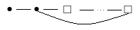
Since and we have
This gives , and so . If , then . The image has self-intersection and arithmetic genus . Therefore, by adjunction , contradicting the fact that is big and nef.
Similarly, if then the has self-intersection and arithmetic genus . By adjunction, we have , contradicting the fact that is nef.
Since all possibilities lead to a contradiction, we conclude that . ∎
We can now prove Theorem 2.6.
Proof of Theorem 2.6.
Now suppose that be a stable surface whose unique non Du Val singularity is a Wahl singularity of length . Let be the minimal resolution of , and let be the minimal model of , which is obtained from by contracting -curves.
Theorem 2.10.
Suppose that is big and nef and satisfies . If is of general type then is a singularity. Moreover, if is a singularity and , then is of general type.
Noether’s inequality (that for surfaces of general type, we have ) implies the following corollary of Lemma 2.4.
Corollary 2.11.
If the surface satisfies , then is not of general type.
The significance of the equality in Theorem 2.10 is that such surfaces lie one above the “Noether line” . That is, is the smallest it can be and still have be of general type.
For the proof of Theorem 2.10, we recall Horikawa’s description of minimal surfaces of general type with in [11]. For , the Hirzebruch surface is the -bundle over whose zero section has self-intersection . We denote by a generic fiber of and note that .
Theorem 2.12.
[11] Let be a minimal algebraic surface with for . Then is the minimal resolution of one of either:
- (1)
() a double cover of branched over a curve of degree 8,
- (2)
() a double cover of branched over a curve of degree 10,
- (3)
a double cover of , where and is even, branched over , or
- (4)
( or ) a double cover of the Hirzebruch surface branched over .
In each case, the branch curve has at most ADE singularities.
We call a surface as in Theorem 2.12 a Horikawa surface. These surfaces are key to the proof of Theorem 2.10.
Proof of Theorem 2.10.
By taking a resolution of Du Val singularities , we can assume that has no Du Val singularities. We first show that if is a singularity and , then is of general type. Since and , we have . Because has length , we have . Thus, . By the Enriques-Kodaira classification, is of general type.
Now suppose that is of general type. Then satisfies Noether’s inequality . On the other hand, by Lemma 2.4, we have . Therefore . Since the maps and in Figure 2 do not affect the invariants and , the surface must be a Horikawa surface. Furthermore, we have that , so by Lemma 2.6, the only possible Wahl singularities on have length 1 or 2.
If is a Wahl singularity of length 2, then the resolution of in is a T-string where, without loss of generality, and . Since , the surface is the blowup of in a single point. Let be the exceptional curve of . We have:
| (4) |
| (5) |
We multiply Equation (5) with and and use that is nef to find that and . On the other hand, if we multiply Equation (4) with and use that is nef, we see that .
If , then , so . Since is bif and nef, the only possibility is that is a -curve. But is singular, so this is not possible.
Now suppose that . Then and . This implies that is a nodal or cuspidal cubic. We will use the fact that is a Horikawa surface to show that in fact such a curve cannot exist on .
By Theorem 2.12, the surface is the minimal resolution of a surface with at most Du Val singularities, which is in turn a double cover of where is either or a Hirzebruch surface . Let be the minimal resolution of and the double cover branched over a curve . See Figure 5.
We must consider four cases, corresponding to the cases in Theorem 2.12. Let , and let be the image of on .
Case I. () Suppose that and , where is a hyperplane class. Then , so
Since is odd, this implies that , so .
But then is a union of smooth curves meeting transversally, one component of which is , whereas is singular.
Case II. () If and , then . In particular is even for any . However, , so this case is impossible.
Case III. Suppose that and where and is even. Then
We know , so if where and are nonnegative, then
Since and is irreducible, there are two possibilities: or . But then in either case, is a union of smooth curves meeting transversally, with as one of the components, whereas is singular. Therefore, this case is impossible.
Case IV. Suppose that and . In this case, . If , where and are nonnegative, then intersecting with implies that . Since is irreducible, we have that , and so . But again, is a union of smooth curves meeting transversally, with as one of the components, whereas is singular, and we have a contradiction.
Therefore the only possible length Wahl singularity on has length 1, so is a singularity. ∎
3. Stable numerical quintic surfaces with a unique singularity
A stable numerical quintic surface is a stable surface with , and . We classify all stable numerical quintic surfaces whose unique non Du Val singularity is a singularity. By Theorem 2.10, the minimal resolution is a minimal surface such that , and , so is a Horikawa surface. Moreover, contains a -curve , the exceptional divisor of . On the other hand, given a Horikawa surface with and and containing a -curve, we can contract to obtain a stable numerical quintic surface with a unique singularity. Thus, the classification of surfaces such as becomes a question of classifying all Horikawa surfaces with and that contain a -curve.
Theorem 2.10 suggests that in order to describe surfaces “one above the Noether line” whose unique non Du Val singularity is a singularity, we might instead describe pairs , where is a Horikawa surface and is a -curve contained in . Because Horikawa surfaces are all described as minimal resolutions of double covers , we can attempt to “find” a curve on a Horikawa surface by describing how such a curve must arise from a curve on intersecting the branch locus in a certain way.
We begin in 3.1 with some notation and basic results about double covers. We then use these results in 3.2 to describe all stable numerical quintic surfaces whose unique non Du Val singularity is a singularity. In 3.3, we count dimensions of a number of loci in of such surfaces, and continue in 3.4 to prove that every stable numerical quintic surface whose unique non Du Val singularity is a singularity lies in the closure of one of two distinguished loci.
3.1. Double covers
Let be a double cover of a smooth surface branched over a curve with at most ADE singularities, and let be the minimal model of , obtained by resolving all Du Val singularities on . Then by [10, Lemma 5], the surface is the double cover of a smooth surface with smooth branch locus obtained as follows:
Let be a singular point of and let be the blowup of at . Let be the exceptional divisor of , and let . Define to be the double cover of branched over . Then there exists a map such that the following diagram is commutative.
If is smooth, then is smooth and so we can take , , and . Otherwise, repeat the process, taking to be a singularity of . In this way, we obtain a map which is a composition of maps where is the blowup of a single smooth point , where is a singular point of .
We remark that the resolution given is not necessarily the log resolution of , because we consider singularities of the curves , as opposed to non-nodal singularities of the preimage of .
Now suppose that is a smooth curve contained in , and let be the proper transform of under the map . We denote by the local intersection multiplicity of and at . If is an ADE singularity of , let be the proper transform of under , and let be the point of such that . Then for some we can rearrange the blowups so that for and for . That is, is the smallest integer for which either is smooth at or does not contain . In addition, all maps blowup points away from , so that
We call the separation number of and note that depends on both the singularity of at as well as how the branches of at intersect .
We state here three lemmas, the proofs of which are almost immediate, which will be useful in Theorem 3.4 below.
Lemma 3.1.
Suppose that is an ADE singularity of and that is smooth. Then . In particular, if is the separation number of , then .
Proof.
We have
as desired. ∎
Lemma 3.2.
Suppose that the branch locus of is reducible and contains an irreducible smooth curve . Let and let be a point of . Let . Then . In particular, the separation number of is equal to the local intersection .
Proof.
Since is smooth and has ADE singularities, any singularity of has either or branches at , of which is locally a smooth one. If has two branches at , then is either an singularity of for odd, a singularity of for odd, or an singularity of . If has branches at , then is a singularity of for even.
In each case, . Since
we have obtained the desired result. ∎
Lemma 3.2 says in particular that if consists of distinct points with separation numbers , then
Given , where , we call the minimal degree of , and take if .
Lemma 3.3.
Suppose that is an singularity of . Then is either or .
Proof.
Note that is unibranched and has multiplicity at . Thus, if the tangent cone of at is transversal to , then . On the other hand, if the tangent cone of at is tangent to , then choose coordinates on so that has local equation . Then is locally given by where has minimal degree .Then is the minimal degree of . Since has minimal degree at least , this implies that . ∎
3.2. The classification
We continue to use the notation of subsection 3.1. Let be a fiber of and an irreducible curve in the linear system on or on .
Theorem 3.4.
There is a one-to-one correspondence between stable numerical quintic surfaces with at most Du Val singularities and a unique singularity, and triples , where for or , has at most ADE singularities, and or intersects as follows:
- (1)
, there exists such that is odd, and has either or singularities along and intersects transversally elsewhere. Moreover,
- (a)
if two singularities of are contained in , then each singularity has separation number , and either or .
- (b)
if one singularity of is contained in , then has separation number , and either or .
Figures 6, 7, and 8 show all possible ways and may intersect in this case.
- (a)
- (2)
, , and for all , is even.
Figure 9 details the possible ways and may intersect in this case.
- (3)
and .
Proof.
Suppose that is a stable numerical quintic surface whose unique non Du Val singularity is a singularity and let be its minimal resolution. Then is a Horikawa surface with and , containing a -curve . Let be the canonical model of , so that has at most Du Val singularities. By [11], is a double cover of a smooth or singular quadric , with branch locus away from any singularity of . We resolve both singularities of lying over the singularity of . Then there exists a map , where is the double cover of , where or , branched over with at most ADE singularities [11]. We claim that the curve is linearly equivalent to either or .
The canonical class of is linearly equivalent to . Let be a divisor such that . Then since is a double cover, the canonical class is given by . Thus, .
Let . If is not contained in the branch locus , then is either a union of two curves and or , depending upon how the curve intersects the branch locus . More precisely, if and only if the multiplicity of and is even at each point of intersection. We consider the three cases, , , and , separately.
Case I. Suppose that there exists such that is odd. Then and we have
so . Since is irreducible the curve is also irreducible. Thus, . Note that .
On the other hand, since is the double cover of a smooth surface and , the curve is a -curve on . Since has genus and is a double cover, the Riemann–Hurwitz formula gives . Because is smooth, the branch divisor intersects transversally. Commutativity of the diagram
implies that . Noting that and we see that the map blows up exactly two points and on , which may be infinitely near.
Suppose that and are distinct, and let . Then has separation number . Moreover, because is smooth, either intersects transversally at , or and do not intersect at . That is, or . By Lemma 3.1, this implies that or . Conversely, if or , then since is singular, has separation number .
If , then is an singularity of , and any branches of at intersect transversally. See Figures 6(a) and 6(b) for the local intersection of and .
Now suppose that . If is an singularity of for odd, then since , one branch of intersects transversally at while the other intersects at with multiplicity . For , both branches of are tangent to each other, so this is not possible. Thus, is an singularity of and intersects at as in Figure 6(c).
If is an singularity for even, then the tangent cone of at is tangent to . Choose local coordinates on so that has local equation and has local equation where has minimal degree . Then if and only if . In this case, the proper transform of is smooth and transversal to , as desired. See Figure 6(d) for the local picture.
If has a , , or singularity at , then since , the tangent cone of each branch of at must be transversal to . The local intersection of and is shown in Figure 6(e), (f), (g), (h), and (i).
Figure 6 summarizes all possible singularities of along that may occur if blows up two distinct points, as well as how the exceptional curves on intersect and the branch divisor of .
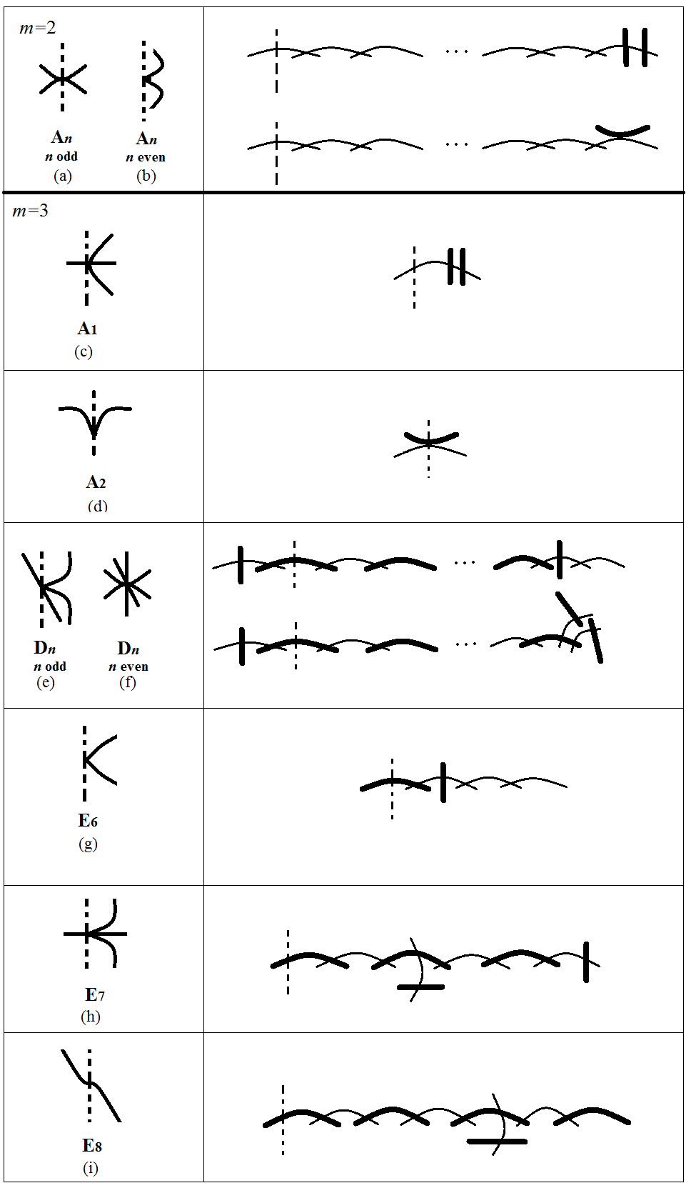
We now consider the case where and are infinitely near. Denote by the center of the the blowup. Then has separation number . Moreover, because the curves and are transversal at , we have or . We show that these two properties (that is, or and having separation number ) hold if and only if and intersect at in one of the ways listed. By Lemma 3.1, if or then has separation number at most . Thus, it is enough to list all possible intersections with or and singular at . We note that for to have separation number greater than 1, at least one branch of at must have tangent cone tangent to .
Our method is to consider the possible singularities of case-by-case, choosing local coordinates at so that the equation of is a standard form (for instance for an singularity and for a singularity). In these coordinates, has local equation or where (or ) has minimal degree , and a simple case-by-case calculation tells us which values of and will give or . We then determine which of these values will give singular at .
Consider the case . Suppose that is an singularity of for odd. If , then is smooth, so has separation number . If , then if and only if
Note that in each case, is singular at , so has separation number .
If is an singularity of for even, then if and only if and . Since , is singular at . Figure 7(d) shows the local intersection of and .
Suppose that is a singularity of for odd and that the singular branch of at has tangent cone parallel to . Since the smooth branch is transversal to , the singular branch interesects with multiplicty . Since is odd and is even, we have . Thus, is a singularity of . See Figure 7(e) for a visualization of how and intersect at . Note that is singular at as desired.
Now suppose that is a singularity of for odd such that the smooth branch of at is tangent to . Then is the minimum of or . Since and , this implies that . The curve is singular at as desired. See Figure 7(f) for the local intersection of and at .
If is a singularity of for even, then two branches of at are transversal to and the third is tangent to with multiplicity . For , two branches of have the same tangent cone, so the branch locus intersects at as in Figure 7(g). The local picture for is similar.
If is an singularity of , then we can choose coordinates so that is the local equation of at and the local equation of at is , where has minimal degree . We quickly see that as desired. The intersection of and at is shown in Figure 7(h).
If is an singularity of , then choose coordinates so that is locally given by and has local equation , where has minimal degree . Then is the minimum of and . But we require , and since , this is impossible.
By Lemma 3.3, is not an singularity.
See Figure 7 for a summary of the ways in which and intersect at if and .

We move on to the case . Suppose that is an singularity of where is odd. If , then the singularity of at is resolved after a single blowup, so we can assume that . Choose coordinates so that the local equation of at is and the local equation of at is where for some . Then in order to have odd, we must have and . Thus , so and . The intersection of and at is shown in Figure 8(a).
If is an singularity of where is even, then is the minimum of and . Thus if and only if and . In this case, has an singularity at . See Figure 8(b) for the local picture.
Next, suppose that is a singularity of where is odd and that the tangent cone of the singular branch is tangent to at . Then we have . Using the same analysis as in previous cases, we see that this case occurs if and only if and . See Figure 8(c) for the local picture.
If is a singularity of for odd such that the singular branch of at has tangent cone transversal to , then the smooth branch is tangent to at with multiplicity . See Figure 8(d) for the local picture.
If is a singularity of where is even, then either two branches of are tangent to at with multiplicity each and the third is transversal, or two are transversal to and the third is tangent to with multiplicity . In the former case, is a singularity and intersects at as in Figure 8(e). In the latter case, has no further restrictions and the local intersection is shown in Figure 8(f).
We showed above that if has an singularity at such that the tangent cone of at is tangent to , then , so we need not consider the singularity in this case.
If is an singularity of , then the same analysis as above shows that is tangent to the tangent cone of at with multiplicity . See Figure 8(g) for the local picture.
Finally, suppose that is an singularity of . An analysis of the local equations of and as above shows that as long as the tangent cone of at is tangent to , we will have . In this case, the proper transform of has a cusp at . See Figure 8(h) for the local picture of and at .
See Figure 8 for a summary of the ways in which and intersect at if and . This completes our discussion of Case I.

Case II. Suppose that and . Then for each point of the multiplicity is even, and are isomorphic, and we have
Suppose that on , we have , where and are nonnegative. Then , so that . Multiplying by , we see that in order for a divisor in the linear system to be irreducible, we must have . Thus, . A similar calculation on shows that in either case .
We now show that if is an irreducible curve in the linear system such that at each point we have even, then is a union of two -curves and .
Suppose that are the singular points of lying on . Let be the separation number of . Then
where the second equality follows from Lemma 3.1. On the other hand
where we again use Lemma 3.1. Thus,
so as desired.
By Lemma 3.1, a singularity of on may be an , , , or singularity, as long as the branches of intersect in such a way that the multiplicity of and at is even. By considering the local equations of each type of ADE singularity, we can determine all possible ways and may intersect, and also have both branches of over smooth. As an example, suppose that has a singularity at . We can choose local coordinates around so that the local equation of is . Since is even, the curve must be tangent to one of the tangent cones of at . We can then write the equation of at as either or where (or ) has minimal degree . Then is the minimal degree of either or . Using the fact that is even, we can then determine the possibilities for and for each such resolve the singularity of as described above. This tells us in particular how intersects the exceptional locus of . The same analysis may be used for the other ADE singularities. See Figure 9 for the list of possible singularities as well as how the curve intersects the exceptional locus of . We remark that this analysis is more general in that it depends only on the fact that both branches of over are smooth, and not on the self-intersection of .

Case III. If then , and so
Since is irreducible, we must have . The fact that implies that where is in the linear system , so . By Lemma 3.2, we have
as desired.
The generic intersects intersect in 10 distinct points and so the double cover has 10 singularities. ∎
3.3. Dimension counts
We begin by showing that every stable numerical quintic surface whose unique non Du Val singularity is a singularity corresponds, up to isomorphism, to a unique triple , where is a quadric surface, is a divisor in , and is the image of the -curve on the minimal resolution of . This observation allows us to count the dimensions of a number of important loci in .
Lemma 3.5.
Suppose that and are the minimal resolutions of stable numerical quintic surfaces and , each of which has a unique singularity and no other non Du Val singularities. Let and be the -curves on and , respectively. Let and be the points of corresponding to and , respectively. The following are equivalent:
- 1)
.
- 2)
There is an isomorphism such that .
- 3)
The triples and corresponding to and are isomorphic; that is, there is an isomorphism such that and .
Proof.
1) 2) is clear.
3) 2) follows by construction of and from the triples given. For 2) 3), suppose that is an isomorphism such that . Let and be the canonical models of and , respectively, and denote by and the images of and , respectively. Then the isomorphism induces an isomorphism of sending to and to . The map is a double cover , where is either a quadric cone or a smooth quadric. Thus, the isomorphism induces an isomorphism . Moreover, if and are the triples corresponding to and under the correspondence of Theorem 3.4, then since , we have and , so the triples are isomorphic. ∎
Let be a singularity on a stable numerical quintic surface , let be its minimal resolution, and let denote the curve on . We call a surface of type
- •
1 if , and and intersect as in Figure 10(d).
- •
1’ if , and and intersect as in Figure 10(e).
- •
1” if , and and intersect as in Figure 10(d).
- •
1”’ if , , there exists with , and and intersect as in Figure 10(f).
- •
2a if , is a fiber, and and intersect as in Figure 10(a).
- •
2a’ if , is a fiber and and intersect as in Figure 10(b).
- •
2a” if , is a fiber, has an singularity along and and intersect as in Figure 10(c).
- •
2b if , is a fiber, and and intersect as in Figure 10(a).

Lemma 3.6.
The stable numerical quintic surfaces of types 1 and 2a correspond to -dimensional loci in . Those of types 1’, 1”, 1”’, 2a’, 2a”, and 2b correspond to -dimensional loci in . All other types of stable numerical quintic surfaces with a unique singularity correspond to loci of dimension less than 38.
Proof.
Lemma 3.5 implies that each triple of Theorem 3.4 corresponds to a unique stable numerical quintic surface, up to automorphisms of . We count the dimension of such triples in the given cases. The main difficulty is to check that requiring that the branch divisor obtain different types of singularities at different points imposes independent conditions on .
To create a triple :
1. Fix a smooth or singular quadric .
2. Choose a divisor or . Then by Riemann-Roch, since and , we have if and if . Projectivizing gives a 3-dimensional space of choices if and a -dimensional space if .
3. Choose points on (through which will eventually pass). Since , we have a -dimensional space of choices for these points. (If is a cone, we can choose the points so that none of them are the singularity of .)
4. Choose a divisor :
- 4a.
To obtain , choose . Again by Riemann-Roch, . Projectiving gives a 48 dimensional space of possible branch curves .
- 4b.
To obtain , choose . By Riemann-Roch, . Projectivizing gives a -dimensional space of possible branch curves . By abuse of notation, take (and note that the resulting triple will be of the form , or with our abuse of notation, ).
5. Consider the restriction exact sequence
By Kodaira vanishing, . Thus, the map
is surjective, and so we can find a curve (or ) such that the restriction of to passes through any points on , counted with multiplicities, where . Thus, the requirement that pass through the given points, counted with multiplicities, is a codimension condition.
6. The group of automorphisms of is -dimensional if is smooth and -dimensional if is a cone. Thus, modding out by automorphisms of is either a codimension condition or codimension condition.
Triples where give a locus of dimension at most , so we can assume for the rest of the proof that .
7. So far there is no guarantee that the most general is smooth at any given point, nor is it immediate that imposing the condition that obtain a certain mild singularity at a given point does not impose conditions on at the other points. Provided the multiplicity at each point is small enough, the fact that these conditions are linearly independent follows from the fact that is sufficiently big. That is, for , the divisor is big and nef, so the cohomology group is zero by Kodaira vanishing. Thus, the map
induced by the restriction is surjective. This means that we can choose in such a way that we can require the degree parts of the “Taylor expansion” of its equation
to be of any form we desire, where is the equation of and .
Suppose we want to impose the condition that acquires a node at a given point for which . This is equivalent to requiring that the linear term in its Taylor expansion vanish at , and that the discriminant of the quadratic term be non-vanishing at . Therefore, this condition has expected codimension . Since this is a requirement on the degree and parts of the Taylor expansion, taking implies that the requirements that be either smooth or obtain at most a node at each of its points are linearly independent conditions. That is, the condition that acquire a node at a point with multiplicity is indeed a codimension condition.
Similarly, the requirement that acquire an singularity at a point for which is equivalent to requiring that the linear term in its Taylor expansion vanish at , the discriminant of the quadratic term also vanish at , and the cubic term be nonvanishing. Since this is a requirement on the part of the Taylor expansion of degrees , , and , taking implies that acquiring an singularity at the desired point is a codimension condition.
Requiring to have a node at a point for which is equivalent to forcing the linear term in its Taylor expansion to vanish at , and the coefficient of one monomial in the quadratic term to vanish at . Again, this is a requirement on the degree part of the Taylor expansion, so taking implies that this is a codimension condition that does not impose conditions on the other points of .
Let be the dimension of the set of triples such that (set theoretically). Then
Thus, if is the codimension of the set of triples such that has prescribed singularities, then in order for the set of such triples to have dimension or , we have
.
In particular, we see that if , then since , we have or . If , then since , we have .
For instance, the dimension of the locus of type 1 surfaces is , and of type 1’ surfaces is .
The dimension of the locus of type 2a surfaces is , and of type 2b surfaces is .
Working through each of the remaining possibilities in Theorem 3.4 gives the desired result. ∎
3.4. The closures of the loci of type 1 and 2a surfaces
The goal of this subsection is to prove the following.
Theorem 3.7.
Let be a stable numerical quintic surface corresponding to the triple , and let denote its corresponding point in . If , then is in the closure of the locus of 2a surfaces. If , then is in the closure of the locus of surfaces of type 1. Thus, the closures of the loci of surfaces of types 1 and 2a contain all surfaces whose unique non Du Val singularity is a singularity.
We begin by showing that if is a surface corresponding to the triple for (respectively, ) then there is a family of triples with special fiber whose general fiber is a triple corresponding to a surface of type 1 (respectively, 2a). We then take a double cover of branched over , followed (after a possible finite base change) by a simultaneous resolution of Du Val singularities. Ideally, this would give the minimal resolution of the desired family of stable numerical quintic surfaces, and then contracting a section of curves would give the family itself. However, we may first need to do a sequence of flops in order to guarantee existence of a family of -curves with irreducible special fiber. The bulk of the work is showing that such a sequence exists.
Lemma 3.8.
Let be a triple corresponding to a stable numerical quintic surface. If (respectively, ), then is the special fiber of a family of triples with general fiber a triple corresponding to a stable numerical quintic surface of type 1 (respectively, 2a).
Proof.
Suppose that and consider the restriction sequence
Since , the induced map
is surjective.
Let be the locus of effective divisors with at most Du Val singularities, and let be the locus of effective divisors consisting of six distinct points. Note that is open in and is open in . Let be the map sending a section to its square. Projectivizing, we obtain an injective map which sends an effective divisor to the divisor . Being a projective map, the map is a closed. Therefore,
That is, the locus of branch divisors with at most Du Val singularities that intersect in any six points, with even multiplicities, is the closure of the locus of branch divisors with at most Du Val singularities that intersect in six distinct points with multiplicity two at each point.
A similar argument holds for , where we consider instead the restriction map
take to be the locus of effective divisors consisting of four distinct points, two of which have multiplicity two, and take to be the identity map. ∎
Suppose that is a Du Val singularity of on , and let be the exceptional divisor of over . Let denote the corresponding root lattice of type , , or , with positive-definite inner product . Note that is the negative of the intersection product on the Picard group of . That is,
Let be the corresponding weight lattice, where are the fundamental weights, satisfying . By means of the inner product, we identify with a lattice in , and in this way think of as a sublattice of . In particular, we may extend in a unique way the inner product on to .
Given any effective divisor , we can associate to the weight satisfying
for all . As an example, if is a divisor such that for some we have and for , then under this correspondence, we have .
We will use the classification of Theorem 3.4 to describe all ways the -curve intersects the exceptional divisor . We label the dual graphs of the exceptional divisor of a Du Val singularity as follows:
It will be useful to have a description of the root systems , , and .
For , let be an orthonormal basis of . A basis of simple roots of is given by .
For , we let be an orthonormal basis of . A basis of simple roots is given by for and .
To describe the root system of , let be a Del Pezzo surface given by the blowup of in points in general position. Then the root lattice can be described as the orthogonal complement of the canonical class in , after a sign change. Let be a basis of , where are classes of the exceptional curves on , and is the pullback of a hyperplane section. We note that . With respect to the pairing satisfying , , and (the negative of the intersection pairing on ), we can describe the simple roots of as
Our main tool for proving the existence of the desired sequence of flops is the following.
Lemma 3.9.
Let be a family of surfaces over the unit disk in with special fiber . Let be a divisor whose restriction to is an effective sum of curves , where the are distinct -curves, and for all . Suppose there exists such that . Let be the flop of . Then
where . That is, flopping the curve results in a divisor with at least one fewer -curve on the special fiber.
Proof.
Suppose that is negative. Flopping does not change the coefficients for , and so
for some nonnegative integer . Moreover, because , flopping gives . Thus
so
Since , we have that . ∎
Lemma 3.10.
Let be a family of triples over the unit disk in , with general fiber corresponding to a stable numerical quintic surface of type 2a or 2b and such that is a ruling. Let be the double cover of branched over . Then there exists, after a possible finite base change, a simultaneous resolution of singularities such the closure of the -curve on the general fiber is irreducible.
Proof.
Let be a triple corresponding to a stable numerical quintic surface, and suppose that is a ruling. Let be a family of triples whose general fiber is of type 2a or 2b, and whose special fiber is the triple . Consider the maps
where is the double cover branched over , and is any simultaneous resolution of Du Val singularities, which exists after a possible finite base change. Let be the closure of the -curve on the general fiber of . Recall that has two nodes lying on the general fiber of , and thus the general fiber of contains two curves intersecting the general fiber of . Let and be the closures of these -curves. We claim that there exists a sequence of flops of so that has irreducible special fiber.
Let be the -curve on and let exceptional divisor over the singularities of on . Then
where
and the are nonnegative integers. Since the general fibers of and are disjoint -curves, the divisors and satisfy and . Moreover
| (6) |
We pass to the weight lattice of the corresponding singularity (or singularities) on . Note that if has one singularity on , then is irreducible. But if has two singularities, then the lattice is a direct sum of irreducible lattices, each corresponding to a singularity of on . In either case, Equation (6) implies that the weight
is equal to . Thus, as weights, we have
We prove that if for all , then for all . Together with this, Lemma 3.9 implies that if for some , then there exists a flop of after which will contain at least one fewer -curve.
Suppose that for all , we have . Passing again to the weight lattice, this is the statement that
for all . The last inequality is equivalent to the statement that the weight
is dominant. We therefore have
where equality holds if and only if for all . Thus, our proof is complete once we show that independent of the singularity (or singularities) of on .
By Theorem 3.4, and referring to Figures 6, 7, and 8, we have the following table detailing how intersects the curves . We write to denote the weight restricted to the irreducible lattice corresponding to the singularity of , and note that if is irreducible (i.e., if has only one singularity on ), then . Otherwise, where and are orthogonal weights in , each corresponding to a singularity of on .
| Singularity | Nonzero intersections | ||
| 2 | |||
| 3 | |||
| 3 | |||
| 3 | |||
| 3 | |||
| 3 | |||
| 3 | |||
| 4 | , | ||
| 4 | |||
| 4 | |||
| 4 | |||
| 5 | |||
| 5 | |||
| 5 | , | ||
| 5 | |||
| 5 | |||
| 5 |
One quickly checks that if is or , then and if is or , then . In the former case, is the sum of two perpendicular vectors and , and thus
This completes the proof. ∎
Remark 3.11.
In the case where is a diagonal, have a more general statement. The proof will require the following.
Lemma 3.12.
[3, VIII, 7.3] Let be a weight and suppose that is dominant. Then the weight is a (dominant) weight of the irreducible representation of highest weight of the corresponding Lie algebra.
A weight is minuscule if it is the only dominant weight of .
Theorem 3.13.
Let be a smooth surface, a divisor on with at most Du Val singularities, and a smooth irreducible divisor on . Let be a family of triples over the unit disk in , with special fiber , and such that the divisors and are reduced, irreducible and smooth for . Suppose that at each point over the general fiber, the local intersection is even. Let be the double cover branched over . Then there exists, after a possible finite base change, a simultaneous resolution of singularities such that the closure of one of the two components of over the general fiber has irreducible special fiber.
Proof.
We can work locally, so we assume that has a unique singularity at . Let be the double cover branched over and a simultaneous resolution of Du Val singularities of , which exists after a possible finite base change. Let and be the closures in of the two components of over the general fiber. Note that
where is the exceptional divisor over , is the special fiber of , is the special fiber of , and the and are nonnegative integers. If the special fiber of either or is irreducible, that is, if either all or all are zero, then we are done. Otherwise, we claim that there exists a sequence of flops so that has irreducible special fiber. As in the proof of Lemma 3.10, we show that if for all , then for all . We then apply Lemma 3.9 to prove the claim.
Suppose that for all . Passing to the weight lattice, this is equivalent to the statement that the corresponding weight is dominant. By Lemma 3.12, we have that is a dominant weight of the irreducible representation . If is minuscule, then this implies that for all and we are done. We refer the reader to Figure 9, which details all possible ways that and may intersect at together with how intersects the exceptional curves on and the branch divisor of . This gives the following table of weights , depending on the singularity of at .
| Singularity | |
|---|---|
| for any | |
One can check that these are all minuscule fundamental weights. ∎
Remark 3.14.
The proof of Theorem 3.13 relies on the definition of a minuscule fundamental weight. It is interesting to note that the table at the end of the proof contains all minuscule fundamental weights of the simple Lie algebras.
We can now prove the main theorem of this section.
Proof of Theorem 3.7.
Let be a stable numerical quintic surface corresponding to the triple , and let denote its corresponding point in . By Lemma 3.8, there exists a family of triples over the unit disk in such that and if (respectively, ), then the general fiber of is a triple corresponding to a stable numerical quintic surface of type 2a (respectively, type 1). Let be the double cover of branched over , and let be a simultaneous resolution of singularities of , which exists after a possible finite base change. Let be the closure of (one of the) -curve(s) on the general fiber of . By Lemma 3.10 and Theorem 3.13, there exists a sequence of flops so that has irreducible special fiber. Contracting results in the desired family of stable numerical quintic surfaces. ∎
4. Deformations of surfaces of types 1 and 2a
We describe the components of corresponding to surfaces of types 1 and 2a and show that their closures are generically Cartier divisors in the boundary of the type I and IIa components of . In Lemma 3.6, we showed that these components are both -dimensional. In 4.1, we construct explicit -Gorenstein families of numerical quintic surfaces to show that these components are in the boundary of the respective components on . In 4.2, we prove a number of technical results which we use in 4.3 to show that the closures and of these components are generically Cartier divisors. In particular, we show that the cohomology groups controlling obstructions to -Gorenstein deformations of surfaces of types 1 and 2a vanish.
4.1. Families of stable quintic surfaces
4.1.1. Type 1
We describe a family of quintic surfaces degenerating to a stable numerical quintic surface of type 1.
Theorem 4.1.
Consider the family of surfaces
where is the unit disk in and and are forms of degrees , and , respectively, such that
- •
is a smooth quintic surface for
- •
is the union of a smooth double quadric given by and a plane given by intersecting transversally.
For general and , the KSBA stable limit of the family is a stable numerical quintic surface of type 1. Conversely, any stable numerical quintic surface of type is the stable limit of such a family.
Proof.
The singular locus of is the surface , so is not normal. To compute the stable limit we first normalize the family. After normalization and an extremal contraction, we will see that the family of surfaces obtained has reduced special fiber and ample canonical class.
Let be the normalization of . We determine the structure of . First note that the normalization is an isomorphism away from .
Let be a complex analytic neighborhood in of a point . Then on , we can write
where the subscripts indicate the degree of each term in linear coordinates centered at . Giving weight 1, we can write the equation of as
Let be the “discriminant curve” given by . If , then the equation of factors into the product of two linear terms which are not equal. That is, is locally analytically isomorphic to a threefold . Thus, over the open set , the special fiber is an unramified double cover of .
Now consider a point . The equation of may be written locally analytically as
Thus, in order to determine the structure of near , we must consider the degree three part of :
Suppose first that . Then we may assume that and complete the square in the first few terms of :
Let and note that is a linear form. This last equation now becomes
where
and
are linear forms. Finally we can rewrite this as
where is a linear form. Thus, in a complex analytic neighborhood of any point , the threefold is locally analytically isomorphic to the threefold which is the product of with the Whitney umbrella, or pinch point. The normalization of is with normalization map . Here, the quadric corresponds to the locus , so away from , the normalization of is the double cover of the smooth quadric , ramified along the discriminant curve . Since is a curve of degree 12, the surface is the double cover of , ramified along a divisor in the linear system .
Next, we consider a point . We begin by assuming that . Then and , so we can assume that and we have
By choosing sufficiently general, we can assume that and so take . Thus, factors as
The linear term of each factor is unique up to multiplication by a nonzero constant. In particular, the second factor does not vanish identically along . Since the first term must vanish along . Thus, the normalization of is an unramified double cover of , of which one component (the component corresponding to the first factor of above) contains the entire proper transform of .
For the six points , we have and . We suppose first that is a smooth point of . Then we can assume that and so we can write the local equation of as
Completing the square gives
Let and note that we can write . Then can be rewritten in terms of as
Thus, the threefold is again locally analytically isomorphic to the threefold which is the product of with the Whitney umbrella. The normalization of is with normalization map . In the coordinates of the plane corresponds to the plane . Because the normalization is an isomorphism over this locus, we have is the plane given by . The quadric corresponds to the locus , which under the normalization becomes the plane . Thus, we see that the proper transforms and of and intersect transversally after the normalization.
The plane intersects the quadric in a conic . Thus, for general , and , the curve intersects the locus tangentially at 6 points. Taking the double cover of branched over gives a smooth surface with a smooth -curve given by the intersection of the plane with the surface .
We now show that an extremal contraction of results in a family of surfaces with ample canonical class. The canonical class is given by . Since and
we see that can be contracted and that the surface obtained after contracting gives the stable limit. Note moreover that is a -curve on , so this contraction produces a singularity on . By construction, the stable limit of the family is a stable numerical quintic surface with a singularity of type 1 if is smooth, and of type 1’ if has a node on .
We claim that any stable numerical quintic surface of type 1 may be obtained as the stable limit of such a family. By Lemma 3.5, it suffices to show that given any triple (where is a fixed smooth quadric, and are smooth, and such that intersects with multiplicity at points) we can find a family of the desired form whose stable limit is a stable numerical quintic surface corresponding to under the correspondence of Theorem 3.4.
Fix such a triple. Then is isomorphic to a smooth quadric in given by . Let be the equation of the hyperplane in such that . We claim that is also given by , where is a hypersurface of degree in . To see this, let be a general hyperplane section of and consider the exact sequence
Since , we see that global sections of surject onto global sections of . Noting that , this implies that the element can be lifted to a hypersurface of degree in , proving the claim.
Next consider the exact sequence
Since intersects at points with multiplicity each, this implies that the equation of is of the form , where the six points of are given by . Therefore can be chosen to have equation , where is a general form of degree . Then taking
gives the desired family. ∎
Remark 4.2.
We remark that the family given in Theorem 4.1 is one case of a more general degeneration of Castelnuovo surfaces (minimal surfaces of general type with whose canonical maps are birational onto their images) described by Ashikaga and Konno [2, 2.3]. Indeed, the family they give is the minimal resolution of the -Gorenstein family we described in the proof of Theorem 4.1.
4.1.2. Types 2a and 2b
Friedman [7] constructed a family of stable numerical quintic surfaces with general fiber a numerical quintic surface of type IIb and special fiber a stable numerical quintic surface of type 2b. His construction easily generalizes to give a family of stable numerical quintic surfaces whose general fiber is a numerical quintic surface of type IIa and with special fiber a stable numerical quintic surface of type 2a.
Theorem 4.3.
[7] There is a -Gorenstein deformation , where is the unit disk in , with general fiber , , a smooth numerical quintic surface of type IIa (respectively, IIb) and special fiber a stable numerical quintic surface with a singularity of type 2a (respectively, 2b). Furthermore, this deformation induces a versal local -Gorenstein deformation of a singularity.
We omit the proof of Theorem 4.3, but make two important observations. The first is that Friedman’s construction is a degeneration of a family of IIb surfaces to a 2b surface. The construction of a family of IIa surfaces degenerating to a 2a surface is similar. For details, see [19].
Secondly, we remark that Friedman’s family induces a versal local -Gorenstein deformation of the singularity on the special fiber. To see this, note that if is a germ of a singularity, then is analytically isomorphic to the singularity
Moreover, any deformation of is analytically isomorphic to a deformation of the form
for some integer called the axial multiplicity of the deformation. The resolution of the total space of such a deformation consists of two components intersecting with multiplicity . A versal local -Gorenstein deformation of has axial multiplicity ; that is, its resolution consists of two components meeting transversally. The special fiber of Friedman’s family consists of two components meeting transversally and therefore induces a versal local -Gorenstein deformation of the singularity.
Remark 4.4.
In [7, Corollary 1.2], Friedman uses Horikawa’s description of the moduli space to deduce the existence of a -Gorenstein family of smooth quintic surfaces whose special fiber is an “accordion” of surfaces where is the minimal resolution of a stable quintic surface of type 2b, are copies of , and is a copy of , intersecting transversally as in Figure 11.

Here, the canonical class is not ample, and the stable limit of is obtained by contracting the surfaces . We now recognize the resulting special fiber as a stable numerical quintic surface of type 2b. Thus, Friedman’s family is a -Gorenstein smoothing of a 2b surface to a quintic surface. This family gives a local deformation of the singularity with axial multiplicity , so unless , the induced deformation is not versal. Theorem 5.1 in Section 5.4 implies that if is a 2b surface, then there exists a -Gorenstein smoothing of to a quintic surface with .
Friedman also raises the question of describing deformations of 2b surfaces explicitly. Theorem 5.1 answers this question.
4.2. Some sheaf calculations
Let be a smooth surface and a divisor in with simple normal crossings (in particular, each component divisor is smooth). Let denote the sheaf of logarithmic differentials. This sits in the short exact sequence of sheaves
where the map is the residue map.
Now let be a surface whose only non Du Val singularity is a Wahl singularity and let be its minimal resolution. If is the exceptional divisor on , then one can show that obstructions to -Gorenstein deformations of lie in the cohomology group [15]. Thus, if , then the locus of such surfaces is generically smooth in . The calculations of in Theorems 4.8, 4.10, and 5.2 require the following lemmas.
Lemma 4.5.
Let be the blowup of a smooth surface at a point lying in the smooth locus of a divisor with normal crossings. Let be the proper transform of . Then , where is the ideal sheaf of on .
Proof.
It suffices to show the equality in a neighborhood of the exceptional divisor . Let be a coordinate neighborhood around . Choose coordinates on so that is at the origin and the local equation of is . Then is covered by two neighborhoods and . Choose coordinates on so that and the local equation of is . Note that does not appear in . Let coordinates on be so that . On , the local equation of is and the local equation of is . See Figure 12.

On , we have
| (7) | |||||
| (8) |
On
These sections glue to a section of over if coefficients of and are equal:
| (9) |
| (10) |
Replacing in Equation (10) with its equivalent expression coming from Equation (9) yields the equality
From this last expression, we see that
and
where is a polynomial with . Plugging these into Equation (9) and multiplying through by gives
Since the right hand side is a polynomial in , we can write for some polynomial with , and rewrite the above equality as
Therefore, . We now have expressions for , , , and as polynomials in and , which we can use in Equation (8). This gives us
where the only restrictions on and are that neither has a constant term; that is, they both lie in the maximal ideal . Thus,
∎
Lemma 4.6.
Let be a double cover of a smooth surface , and let denote its smooth branch divisor. Let be the preimage of a smooth curve on , and suppose that intersects transversally. Then
and
where . Moreover, these decompositions break the sheaves into their invariant and anti-invariant subspace under the action of by deck transformations.
Remark 4.7.
Proof.
In order to compute , note that it admits an action of via deck transformations, so we can decompose it into its invariant and anti-invariant eigenspaces.
Let be an open neighborhood of and choose coordinates on so that is at the origin and the local equation of is and the local equation of is . Then we have an open neighborhood of with local coordinates so that . Note that the ramification locus of has local equation and the curve on has local equation . See Figure 13.

On we have
Noting that , we have
The action of sends to . Therefore the invariant subspace of is
The anti-invariant subspace of is
One checks easily that these modules extend to the expected sheaves over all of . The proof for the log tangent bundle is similar. ∎
4.3. Smooth boundary components of
We show that loci corresponding to surfaces of type 1 and 2a give generically smooth loci in the moduli space . In both cases, we obtain this result by proving the vanishing of the cohomology group in which obstructions to -Gorenstein deformations lie. By Theorem 3.6, the type 1 and 2a loci are -dimensional, so we conclude that the closure of the 1 and 2a loci are generically smooth Cartier divisors in .
4.3.1. The type 1 component
For this subsection, let be a stable numerical quintic surface of type 1 or 1” and denote by its minimal resolution. Let be the double cover, where or , and is branched over a smooth curve , tangent to at six points. Then and the curves and are curves on . Let denote the ramification locus of , and let be a curve such that .
In order to show that deformations of are unobstructed, it suffices to show that . Equivalently, as described above, we show that .
Theorem 4.8.
Let be the minimal resolution of a stable numerical quintic surface of type 1 or 1”, and let and be the -curves on . Then .
Proof.
By Serre duality, it is enough to show that where .
The double cover gives rise to an action of on via deck transformations. To begin with, we prove that the anti-invariant subspace vanishes.
By the projection formula, noting that , we have
We claim that
To compute , we need only consider a point in . Indeed, suppose that is a neighborhood of such that , and let denote the image of under . By Lemma 4.6, we have
because .
Now let be an open subset of containing , and let an open neighborhood of . Choose coordinates on so that is at the origin and the local equation of is . We can then choose coordinates on such that the local equation of is and the local equation of is . Then the local equations of and are and . With these coordinates, the cover is given by the function . See Figure 14.

The -module is generated by . As a module over , we have that is generated by
Since the action of sends to , we see quickly that the anti-invariant submodule is generated as an –module by
This last module we recognize as . Thus,
By the projection formula, using that , we have
To show that , consider the exact sequence
where is the residue map. Twisting by gives the exact sequence
Looking at the corresponding long exact sequence in cohomology, it remains to show that and . Both of these are obvious, the first because and the second because . Thus,
as we wished to show.
Now consider a one-form . Since
and the latter sheaf has no anti-invariant part, the one-form must be invariant. But the action of on cohomology interchanges and , so must not have a pole along . Thus,
By Horikawa [11], we have , and so , completing the proof. ∎
In Section 3.3, we showed that the locus of stable quintic surfaces of type 1 is -dimensional, so Theorems 4.1 and 4.8 imply the following:
Corollary 4.9.
The closure of the locus of surfaces of type 1 is a generically smooth Cartier divisor in , lying in the closure of the type I component of .
4.3.2. The 2a component
Let be a stable numerical quintic surface of type 2a, 2a’, or 2a” and let denote its minimal resolution. Then there is a map , which is the double cover of the blowup of in two points and lying on a fiber . The branch locus of is the proper transform of an irreducible curve which has either a node or an singularity at each of and and is smooth elsewhere. Denote by and generic rulings of so that , where is the proper transform of .
Theorem 4.10.
Let be a stable numerical quintic surface of type 2a, 2a’, or 2a”, let be its minimal resolution and the -curve on . Then
We begin with a lemma.
Lemma 4.11.
Proof.
We have the following exact sequence of sheaves on :
where is the residue map. Twisting by gives the exact sequence
| (11) |
Note that
| (12) |
and so is effective. Thus . Since the irregularity of is zero, we have . Moreover, noting that and , we have
and
Therefore , so the cohomology group
is if and only if the connecting homomorphism
is injective.
Since is effective, we have a section , so we have a map from the short exact sequence (11) to the short exact sequence
where the map is given by tensoring with . The connecting homomorphism
of the corresponding short exact sequence is the first Chern class map. That is, if and are generators of , then and . Thus, the map is injective if and only if the curves and are linearly independent in the Picard group of . Recalling that Pic is generated by , , and , and that and , we see that the two divisors are indeed linearly independent.
Thus, we have a diagram
where the bottom arrow is injective. We see that is injective as long as the map on the left is injective. But this map simply takes a section of and multiplies it by . Since , the map is injective. ∎
Proof of Theorem 4.10.
We show that , where is the minimal resolution of and is the -curve on . By Serre duality, it is enough to show that . Recall that and . By the projection formula
Together with Lemma 4.6, this gives
By Lemma 4.11, we have . It remains to show that , which we do via the projection formula. By Lemma 4.5, we have , where is the ideal sheaf of and which are the centers of . Noting that , the projection formula gives
We have , because for or . And , since and lie on . ∎
By Theorem 3.6, the locus of 2a surfaces is -dimensional. Moreover, Theorem 4.3 shows that every 2a surfaces may be obtained as the stable limit of a family of numerical quintic surfaces of type IIa. Together with Theorem 4.10, this implies the following
Corollary 4.12.
The closure of the locus of surfaces of type 2a is a generically smooth Cartier divisor in , lying in the closure of the type IIa component of
5. Deformations of 2b surfaces
We study the versal -Gorenstein deformation space [8] where is a general 2b surface. All deformation functors considered are functors of Artinian rings. However, because is a stable surface, we often abuse notation and view as an analytic germ of a point in the KSBA moduli space. The same notational ambiguity applies to other deformation functors we consider which admit a moduli space. This enables us to study the moduli space using analytic methods of Horikawa [10, 11]. The main theorem is
Theorem 5.1.
The locus of stable numerical quintic surfaces whose unique non Du Val singularity is a singularity forms a divisor in which consists of two 39-dimensional components and meeting, transversally at a general point, in a 38-dimensional component . This divisor is Cartier at general points of the , , and components. These components are the closures of the loci of 1, 2a, and 2b surfaces described at the beginning of Section 3.3. Moreover, the type , , and components belong to the closure of the components in of types I, IIa, and IIb, respectively.
The proof will consist of several pieces. Theorems 4.8 and 4.10 showed that obstructions to deformations of surfaces of types 1 and 2a vanish, and so the closures of their corresponding -dimensional loci in are generically smooth Cartier divisors. In Theorem 5.2, we show that deformations of 2b surfaces are obstructed and that the obstruction space is one-dimensional. This implies that the space of -Gorenstein deformations of a generic 2b surface is a hypersurface singularity. We show that the space of equisingular -Gorenstein deformations of consists of irreducible components and meeting, transversally at a general point, in the component. Together with Horikawa’s description of , and the smoothings described in Theorems 4.1 and 4.3, this implies that the space has two irreducible components.
By Theorem 4.3, there exists a -Gorenstein smoothing of a 2b surface to a numerical quintic surface of type IIb which induces a versal deformation of the singularity. Therefore, the map to local -Gorenstein deformations of the singularity is surjective. This latter space is one-dimensional, and since has two irreducible components, the space is analytically isomorphic to .
The key to Theorem 5.1 is the proof of the fact that the space of equisingular -Gorenstein deformations of a general 2b surface consists of two irreducible components meeting transversally at a general point. This space is isomorphic to the deformation space of pairs , where is the minimal resolution of , containing -curve . In 5.2, we describe a subfunctor of the deformation functor of pairs , and show that this subfunctor has no obstructions. This will imply that the space contains a smooth component corresponding to the 2a locus. Thus, to prove Theorem 5.1, it suffices to show that the degree two part of the Kuranishi map, given by the Schouten bracket, is nonzero and not a square. Horikawa makes a similar argument in [10] and [11]. In 5.3 and 5.4, we extend his work to the log setting.
We use the following notation throughout this section. Let be the minimal resolution of a surface of type 2b. We recall the construction of . Let be the blowup of in two distinct points and lying on a fiber . Denote by and the proper transforms of and a generic fiber, respectively, and let and be the exceptional divisors of . By abuse of notation, we denote by the proper transform of the negative section on . Let be a reduced, irreducible divisor in the linear system on with simple nodes at and and no other singularities. Let be its proper transform and note that for some smooth divisor on . Then is given by the double cover branched over . The curve given by is the -curve on . Moreover contains four -curves: and mapping to , and and mapping to and , respectively. We denote by and the projection maps to .
5.1. The obstruction
To begin with, we show that the obstruction space is one-dimensional.
Theorem 5.2.
Let be the minimal resolution of a 2b surface, and let denote the -curve on . Then .
The proof of Theorem 5.2 requires two lemmas.
Lemma 5.3.
Let and the blowup of in and . Then .
Proof.
The proof is very similar to that of Lemma 4.11.
We have the following exact sequence of sheaves on :
where is the residue map. Twisting by gives the exact sequence
| (13) |
Note that
and so is effective. Thus . Since the irregularity of is zero, we have . Moreover, because and , we have , , and Therefore
so the cohomology group
is if and only if the connecting homomorphism
is injective.
Since is effective, we have a section , so we have a map from the short exact sequence (13) to the short exact sequence
given by tensoring with . The connecting homomorphism
of the corresponding short exact sequence is the first Chern class map. That is, if , , and are generators of , then , , and . Thus, the map is injective if and only if the curves , , and are linearly independent in the Picard group of . Recalling that Pic is generated by , , and , that and that , we see that the three divisors are indeed linearly independent.
Thus, we have a diagram
where the bottom arrow is injective. We see that is injective as long as the map on the left is injective. But this map simply takes a section of and multiplies it by . Since , the map is injective. ∎
Lemma 5.4.
Proof.
Let be the projection map, and suppose that . We have the short exact sequence
The sheaf is free, so . Thus, tensoring with the above short exact sequence yields the new short exact sequence
Since is projective, the sheaf has no global holomorphic sections, and so
The sheaf is isomorphic to , so by the projection formula we have
The divisor satisfies so that is a fixed part of the linear system . Since is the only fiber containing both and , this implies that
completing the proof. ∎
We can now prove the theorem.
5.2. Deformations of pairs and the equisingular locus
Let be the double cover of a smooth surface branched over a smooth curve . Define to be the space of deformations of that are double covers of deformations of . The group acts on by deck transformations, and the sheaf decomposes into invariant and anti-invariant subspaces as
where [18].
Theorem 5.5.
[6] Via the decomposition of into its invariant and anti-invariant subspaces, the deformation space of double covers of deformations of may be identified with the deformation space of deformations of pairs, where is the branch divisor of .
The proof of Theorem 5.5 involves identifying the space of first order infinitesimal deformations of double covers of deformations of with the anti-invariant subspace . Then using the decomposition of above, this space is isomorphic to .
Using Lemma 4.6, the same analysis works in the presence of the curves and , as long as intersects transversally. More explicitly, define to be the functor of Artinian local rings which associates to an Artinian local ring the set of isomorphism classes of deformations over of squares
where the top and bottom maps are double covers and the left and right maps are embeddings of the smooth curves and into and , respectively. Then the functor may be identified with the functor of deformations of triples. The space of first-order infinitesimal deformations of triples is therefore . By Lemma 4.6, we have
There is a forgetful map . This map is an analytic embedding, because the differential
is an isomorphism onto its image.
Suppose now that is a stable numerical quintic surface of type 2b, its minimal resolution, and the curve on . Then we have the commutative square
where is the double cover of , where is the blowup of in two points lying on a fiber . The branch curve of is a smooth curve , which intersects the proper transform of transversally. Deformations of this square can be identified with deformations of the triple . The following lemma shows that in this case, the image of is a neighborhood of in the component of . We note that Lemma 5.3 implies that there are no obstructions, so the image of is smooth.
Theorem 5.6.
Let be a stable family whose fibers are all 2a or 2b surfaces and be its simultaneous minimal resolution over , which exists by [13, Theorem 7.68]. Then there exists a double cover of schemes smooth over , where is a smooth family of Hirzebruch surfaces of type or blown up at two points on a fiber.
Proof.
Let be the canonical model of over . Then the canonical map given by the linear system is a double cover over , where fibers of are either smooth or singular quadrics. Let denote the branch divisor of and suppose that is singular for some . Then because the fibers of are 2a or 2b surfaces, the branch divisor of the map is disjoint from the node in .
Let be a simultaneous resolution of singularities of . Then the simultaneous resolutions and are locally analytically isomorphic in a neighborhood of each singularity of , because the branch divisor does not intersect the singularities of . Thus, no finite base change of is required to construct . Letting denote the double cover of branched over the preimage of , there is a map such that the following diagram is commutative:
Now let denote the preimage of under . On each fiber, has two singularities. Let denote the double section of passing through these singularities, and let be the blowup of in . Then is a simultaneous embedded resolution of singularities of . Thus, no finite base change of is required to construct , and the map defined by is a double cover over . ∎
Thus, the space of equisingular deformations of contains a smooth -dimensional component corresponding to the closure of the 2a locus in .
5.3. Three technical lemmas
Our goal is to describe the degree two part of the Schouten bracket. We use a method similar to [10, 11]. In this section, we prove three technical lemmas, analogous to Lemmas 24, 29, and 31 in [10].
We recall the definition of the Kuranishi deformation space in more generality. Suppose that is a smooth surface, and let be the space of deformations of . The tangent space to , that is the space of first order infinitesimal deformations of , is isomorphic via the Kodaira–Spencer map to the cohomology group . Let be a basis of , and let be a dual basis. Then is locally analytically isomorphic to a subspace of with coordinates , and is given by the kernel of the Kuranishi map , which is a certain infinite series in . Catanese’s article [5] gives an excellent exposition of the construction of the Kuranishi map. For us, the important part is that the degree two part of the Kuranishi map is given by the Schouten bracket, which we now describe.
The Schouten bracket is the bilinear map
defined as the composition of the cup product followed by the Lie bracket . If is the infinitesimal first order deformation corresponding, via the Kodaira–Spencer map, to , then is the cohomology class corresponding to the obstruction to extending the deformation to the second order.
Lemma 5.7.
The map
induced by the surjection is surjective.
Proof.
It suffices to show that
is surjective. To do this, recall that the surface admits an action of via deck transformations. By Lemma 4.6, the sheaf decomposes into invariant and anti-invariant eigenspaces as
| and |
We have a similar decomposition of as follows. By the projection formula, we have
Thus,
| and |
We show that the maps
and
are surjective.
To show the first, we have the exact sequence
and so it suffices to show that . By Serre duality, this is equivalent to the vanishing of . This is the statement of Lemma 5.3.
For the second, note that we have the exact sequence
By Lemma 5.4, we have . Moreover, , and thus the map is surjective as long as . Equivalently, we show that .
We claim that the sheaf fits into an exact sequence as
where is a divisor on and . To see this, note first that . Let be an open neighborhood of the point with coordinates so that has local equation and has local equation . Then the map
is locally given by
Thus the map is surjective. Since is a vector bundle of rank two and is a line bundle, the kernel of the map is a vector bundle of rank one. All such vector bundles are given by for some divisor on . We find by calculating the Chern class of . The determinant line bundle is given by , so . Thus, .
Dualizing the above exact sequence and tensoring with results in the exact sequence
The sheaf on the right has no global sections, since the only section of vanishing at and is zero. Moreover, since every divisor in the linear system is a union of two divisors and . Since there is only one such divisor passing through and , namely the divisor , we have
as we wished to show. ∎
A key ingredient of Horikawa’s description in [11] is a map
where and is a generic fiber of the map .
Lemma 5.8.
Let be a smooth surface with a surjective map such that and let denote a generic fiber of . Suppose that for some smooth divisor on such that and let
be the map induced by the surjection . If the irregularity , , and , then there is a map , defined in [19, 4.8] with the property that .
Proof.
Lemma 5.9.
With the same hypotheses as Lemma 5.8, if then is in the image of the restriction map .
5.4. Proof of the main theorem
We describe the space of -Gorenstein deformations of a general 2b surface .
Lemma 5.10.
[11, Lemma 6.3] Let be the minimal resolution of a surface of type 2b. Then and .
Proof.
Horikawa proves this in the case that is a double cover of with a smooth branch divisor. The proof uses Riemann-Roch and Serre duality together with the fact that the canonical divisor on is given by . Because it only relies on numerical characteristics of , , and , Horikawa’s proof works in our case as well. ∎
By Lemma 5.10, we can define the map as in Lemma 5.8, where . By abuse of notation, we let
be the restriction of this map to . We note that this map is the restriction to of the corresponding map defined in [11] under the assumption that the branch locus is smooth.
Proof of Theorem 5.1.
The deformation space is locally analytically isomorphic to the zero-set of the Kuranishi map
Choose a basis of . Let be the dual basis. A priori, the Kuranishi map is some power series in . However in this case, Theorems 5.6 and 3.6 imply that contains a smooth -dimensional subspace corresponding to deformations of a 2b surface to a 2a surface. This implies that if we choose a basis of such that and for , then the corresponding dual basis has the property that the Kuranishi function factors into at least two terms, one of which has linear term . To show that is locally a product of two smooth -dimensional components meeting transversally in a 38-dimensional component, it therefore suffices to show that the degree two part of the Kuranishi map is nonzero and not a square. The degree two part is given by the Schouten bracket, defined above.
We restrict the Schouten bracket to . We claim that the Lie bracket has image in . Let be a sufficiently fine open covering of and let . Let be an element of , represented by a 2-cocycle , where is a 1-cocycle with coefficients in . Then is a vector field that fixes the ideal sheaf of the . Thus, also fixes the ideal sheaf of . Therefore the Lie bracket gives a vector field on which also fixes the ideal sheaf of . Thus, the form gives a -cocycle with coefficients in ; that is
Because and are dual bases, the degree two part of the Kuranishi map is given by
Moreover, because factors into a product, one term of which has linear term , we have that for . It therefore suffices to show that and is nonzero for some .
Recall that and consider the exact sequence
On , we have and , so the image of the map is one-dimensional. Moreover, the image of is contained in the “diagonal” in . That is, if is a nonzero global section of in the image of , then and . More precisely, we have the commutative diagram below, where the arrow on the left is an isomorphism and the inclusion of into sends a section to the section of whose restrictions to and are equal.
By Lemmas 5.8, 5.10 and 5.7, the map is surjective. Thus, we can choose such that , and is not in the image of . But then is not a restriction of an element of , so by Lemma 5.9, we conclude that . Thus, the Schouten bracket
is surjective.
Because it is locally given by the composition of the cup product followed by the Lie bracket of vector fields, the Schouten bracket is -equivariant under the action of by deck transformations. By Lemma 5.2, the invariant part of is zero, and so is nonzero if and only if is anti-invariant under the action of . Suppose that is an element of , where and are either both invariant or both anti-invariant. Then is invariant, that is . By Lemma 5.2, this space is zero, so . Thus, by choice of basis, for all ; in particular, .
Now suppose that is invariant and is anti-invariant. Then is anti-invariant. Since is surjective, there exists, by choice of basis, such that , completing the proof. ∎
References
- [ALE94] (1994) Boundedness and for log surfaces. Internat. J. Math. 5 (6), pp. 779–810. Cited by: §1.
- [AK91] (1991) Examples of degenerations of Castelnuovo surfaces. J. Math. Soc. Japan 43 (2), pp. 229–246. Cited by: Remark 4.2.
- [BOU08] (2008) Lie groups and lie algebras: chapters 7-9. Springer. Note: English translation Cited by: Lemma 3.12.
- [CAT86] (1986) Connected components of moduli spaces. Differential Geom. 24, pp. 395–399. Cited by: §1.
- [CAT13] (2013) A superficial working guide to deformations and moduli. In Handbook of moduli: Volume I, G. Farkas and I. Morrison (Eds.), Cited by: §5.3.
- [Cv06] (2006) Infinitesimal deformations of double covers of smooth algebraic varieties. Math. Nachr. 279, pp. 716–726. Cited by: Theorem 5.5.
- [FRI83] (1983) A degenerating family of quintic surfaces with trivial monodromy. Duke Math. J. 50 (1), pp. 203–214. Cited by: §1, §1, §4.1.2, Theorem 4.3, Remark 4.4.
- [HAC04] (2004) Compact moduli of plane curves. Duke Math. J. 124 (2), pp. 213–257. Cited by: §5.
- [HAC12] (2012) Compact moduli of surfaces of general type. Contemp. Math. 564, pp. 1–18. Cited by: §1.
- [HOR75] (1975) On deformations of quintic surfaces. Invent. Math. 31, pp. 43–85. Cited by: §1, §1, §3.1, §5.3, §5.3, §5, §5, Abstract..
- [HOR76] (1976) Algebraic surfaces of general type with small , I. Ann. of Math. 104, pp. 357–387. Cited by: §1, §1, Theorem 2.12, §2, §3.2, §4.3.1, §5.3, §5.3, §5.3, §5.4, Lemma 5.10, §5, §5.
- [KAW92] (1992) Moderate degenerations of algebraic surfaces. In Complex algebraic varieties: Proceedings of a conference held in bayreuth, germany, april 2–6, 1990, K. Hulek, T. Peternell, M. Schneiderm, and F. Schreyer (Eds.), Lecture Notes in Mathematics, Vol. 1507, pp. 113–132. Cited by: §1, Remark 2.5, §2.
- [KM98] (1998) Birational geometry of algebraic varieties. Cambridge University Press. Cited by: §2, Theorem 5.6.
- [KS88] (1988) Threefolds and deformations of surface singularities. Invent. Math. 91, pp. 299–338. Cited by: §1, §1, §2.
- [LP07] (2007) A simply connected surface of general type with and . Invent. Math. 170, pp. 483–505. Cited by: §4.2.
- [LP11] (2011) A construction of horikawa surface via -gorenstein smoothings. Math. Z. 267, pp. 15–25. Cited by: Remark 2.7.
- [LEE99] (1999) Numerical bounds for degenerations of surfaces of general type. Internat. J. Math. 10, pp. 79–92. Cited by: §1, Theorem 2.3.
- [PAR91] (1991) Abelian covers of algebraic varieties. J. Reine Angew. Math. 417, pp. 191–213. Cited by: Remark 4.7, §5.2.
- [RAN14] (2014) Boundary divisors in the moduli space of stable quintic surfaces. Ph.D. Thesis. Cited by: §4.1.2, §5.3, §5.3, Lemma 5.8.
- [REI97] (1997) Chapters on algebraic surfaces. In Complex algebraic geometry, ias/park city mathematics series, pp. 3–157. Cited by: §2.
- [VAK06] (2006) Murphy’s law in algebraic geometry: badly-behaved deformation spaces. Invent. Math. 164, pp. 569–590. Cited by: §1.
- [WAH81] (1981) Smoothings of normal surface singularities. Topology 20, pp. 219–246. Cited by: §1, Proposition 2.1, Lemma 2.2, §2.