Leibniz-Institute for Astrophysics Potsdam (AIP)
\university\crest
\degreeDoctor of Natural Science
\degreedate2013
The XMM-Newton/SDSS Galaxy Cluster Survey
Abstract
Galaxy clusters are the largest known gravitationally bound objects, their study is important for both an intrinsic understanding of their systems and an investigation of the large scale structure of the universe. The multi-component nature of galaxy clusters offers multiple observable signals across the electromagnetic spectrum. At X-ray wavelengths, galaxy clusters are simply identified as X-ray luminous, spatially extended, and extragalactic sources. X-ray observations offer the most powerful technique for constructing cluster catalogues. The main advantages of the X-ray cluster surveys are their excellent purity and completeness and the X-ray observables are tightly correlated with mass, which is indeed the most fundamental parameter of clusters. In my thesis I have conducted the 2XMMi/SDSS galaxy cluster survey, which is a serendipitous search for galaxy clusters based on the X-ray extended sources in the XMM-Newton Serendipitous Source Catalogue (2XMMi-DR3). The main aims of the survey are to identify new X-ray galaxy clusters, investigate their X-ray scaling relations, identify distant cluster candidates, and study the correlation of the X-ray and optical properties. The survey is constrained to those extended sources that are in the footprint of the Sloan Digital Sky Survey (SDSS) in order to be able to identify the optical counterparts as well as to measure their redshifts that are mandatory to measure their physical properties. The overlap area between the XMM-Newton fields and the SDSS-DR7 imaging, the latest SDSS data release at the starting of the survey, is 210 deg2. The survey comprises 1180 X-ray cluster candidates with at least 80 background-subtracted photon counts, which passed the quality control process.
To measure the optical redshifts of the X-ray cluster candidates, I used three procedures; (i) cross-matching these candidates with the recent and largest optically selected cluster catalogues in the literature, which yielded the photometric redshifts of about a quarter of the X-ray cluster candidates. (ii) I developed a finding algorithm to search for overdensities of galaxies at the positions of the X-ray cluster candidates in the photometric redshift space and to measure their redshifts from the SDSS-DR8 data, which provided the photometric redshifts of 530 groups/clusters. (iii) I developed an algorithm to identify the cluster candidates associated with spectroscopically targeted Luminous Red Galaxies (LRGs) in the SDSS-DR9 and to measure the cluster spectroscopic redshift, which provided 324 groups and clusters with spectroscopic confirmation based on spectroscopic redshift of at least one LRG. In total, the optically confirmed cluster sample comprises 574 groups and clusters with redshifts (), which is the largest X-ray selected cluster catalogue to date based on observations from the current X-ray observatories (XMM-Newton, Chandra, Suzaku, and Swift/XRT). Among the cluster sample, about 75 percent are newly X-ray discovered groups/clusters and 40 percent are new systems to the literature.
To determine the X-ray properties of the optically confirmed cluster sample, I reduced and analysed their X-ray data in an automated way following the standard pipelines of processing the XMM-Newton data. In this analysis, I extracted the cluster spectra from EPIC(PN, MOS1, MOS2) images within an optimal aperture chosen to maximise the signal-to-noise ratio. The spectral fitting procedure provided the X-ray temperatures (0.5 - 7.5 keV) for 345 systems that have good quality X-ray data. For all the optically confirmed cluster sample, I measured the physical properties ( erg s-1) and ( M⊙) from an iterative procedure using published scaling relations. The present X-ray detected groups and clusters are in the low and intermediate luminosity regimes apart from few luminous systems, thanks to the XMM-Newton sensitivity and the available XMM-Newton deep fields
The optically confirmed cluster sample with measurements of redshift and X-ray properties can be used for various astrophysical applications. As a first application, I investigated the relation for the first time based on a large cluster sample of 345 systems with X-ray spectroscopic parameters drawn from a single survey. The current sample includes groups and clusters with wide ranges of redshifts, temperatures, and luminosities. The slope of the relation is consistent with the published ones of nearby clusters with higher temperatures and luminosities. The derived relation is still much steeper than that predicted by self-similar evolution. I also investigated the evolution of the slope and the scatter of the relation with the cluster redshift. After excluding the low luminosity groups, I found no significant changes of the slope and the intrinsic scatter of the relation with redshift when dividing the sample into three redshift bins. When including the low luminosity groups in the low redshift subsample, I found its relation becomes flatter than the relation of the intermediate and high redshift subsamples.
As a second application of the optically confirmed cluster sample from our ongoing survey, I investigated the correlation between the cluster X-ray and the optical parameters that have been determined in a homogenous way. Firstly, I investigated the correlations between the BCG properties (absolute magnitude and optical luminosity) and the cluster global properties (redshift and mass). Secondly, I computed the richness and the optical luminosity within of a nearby subsample (, with a complete membership detection from the SDSS data) with measured X-ray temperatures from our survey. The relation between the estimated optical luminosity and richness is also presented. Finally, the correlation between the cluster optical properties (richness and luminosity) and the cluster global properties (X-ray luminosity, temperature, mass) are investigated.
{Zusammenfassung}Im Rahmen dieser Arbeit habe ich die 2XMMi/SDSS Galaxienhaufendurchmusterung erstellt (2XMMi/SDSS galaxy cluster survey), eine Suche nach Galaxienhaufen welche auf der Detektion ausgedehnter Röntgenquellen im XMM-Newton Quellenkatalog (2XMMi-DR3) basiert. Die Hauptziele dieser Suche sind die Identifizierung bisher unbekannter röntgenheller Galaxienhaufen, die Erforschung ihrer Beziehungen zwischen Röntgenleuchtkraft und Temperatur (X-ray scaling relation), eine Entdeckung von möglichen weit entfernten Galaxienhaufen und die Beziehung zwischen Eigenschaften im Optischen und Röntgenbereich. Die Durchmusterung ist für alle Quellen der Himmelsregionen ausgelegt, die vom Sloan Digital Sky Survey (SDSS) erfasst werden. Das Ziel besteht darin, ihre optischen Gegenstücke zu finden und deren Rotverschiebungen zu bestimmen. Die gemeinsamen Himmelsareale zwischen XMM-Newton und dem Bildmaterial vom SDSS-DR7 umfassen 210 deg2. Meine Durchmusterung enthält 1180 mögliche Galaxienhaufen mit wenigstens 80 vom Hintergrund bereinigten Photonen im Röntgenbereich, die einer Qualitätskontrolle erfolgreich standgehalten haben.
Um die Rotverschiebungen der möglichen Galaxienhaufen im optischen Bereich zu bestimmen nutzte ich drei Vorgehensweisen: (i) Ein Abgleich jener Kandidaten mit den neuesten und umfangreichsten Katalogen optisch ausgewählter Galaxienhaufen, die in der Literatur verfügbar sind. (ii) Ich entwickelte einen Algorithmus, um Rotverschiebungen der optischen Gegenstücke aus Daten vom SDSS-DR8 zu ermitteln, welches zu photometrischen Rotverschiebungen von 530 Galaxiengruppen-/haufen führte. (iii) Ein weiterer von mir entwickelter Algorithmus nutzte die spektroskopischen Rotverschiebung von roten leuchtkräftigen Galaxien (LRGs) in den Daten des SDSS-DR9 und ergab 324 Gruppen und Haufen. Zusammengefasst enthält diese Probe 574 auch im optischen nachgewiesener Galaxiengruppen und -haufen mit bekannten Rotverschiebungen () - der zur Zeit umfangreichste Katalog von im Röntgenbereich ausgewählten Galaxienhaufen basierend auf aktuellen Röntgenbeobachtungen. Unter jenen Haufen waren ca. 75% im Röntgenbereich nicht bekannt und 40% fanden in der bisherigen Literatur noch keine Erwähnung.
Um die Röntgeneigenschaften der im Optischen bestätigten Haufen zu bestimmen, war eine automatische Reduktion und Analyse der Röntgendaten unverzichtbar. Die Prozedur, welche Modelle an die Röntgenspektren anpasste, ergab Temperaturen von keV für 345 Kandidaten. Für alle Haufen, die auch im optischen auffindbar waren, bestimmte ich die physikalischen Eigenschaften erg s-1) und M⊙).
Die Probe optisch bestätigter Galaxienhaufen mit gemessenen Rotverschiebungen und Röntgeneigenschaften kann für viele astrophysikalische Anwendungen genutzt werden. Als eine der ersten Anwendungen betrachtete ich die Beziehung zwischen ; das erste Mal für eine so grosse Anzahl von 345 Objekten. Der aktuelle Katalog enthält Gruppen und Haufen, die einen grossen Bereich in Rotverschiebung, Temperatur und Helligkeit abdecken. Der Anstieg jener Beziehung ist im Einklang mit bereits publizierten Werten für nahegelegene Galaxienhaufen von hoher Temperatur und Helligkeit. Nach dem Ausschluss leuchtschwacher Gruppen und der Einteilung der Daten in drei nach Rotverschiebung geordneter Gruppen, waren keine signifikanten Änderungen von Anstieg und intrinsischer Streuung zu beobachten.
Als zweite Anwendung unserer Durchmusterung, untersuchte ich die Haufen bezüglich deren Eigenschaften im Optischen und im Röntgenbereich. Zuerst
betrachtete ich den Zusammenhang zwischen den Eigenschaften (absolute Helligkeit und optische Leuchkraft) der hellsten Haufengalaxie (BCG) mit denen
des Haufens als Ganzem (Rotverschiebung und Masse). Danach berechnete ich die Reichhaltigkeit der Galaxienhaufen und deren optische Leuchtkraft
innerhalb von für eine Stichprobe nahegelegener Haufen (, hier sind SDSS Daten noch empfindlich genug um den Grossteil
der Haufengalaxien abzubilden) mit gemessenen Röntgentemperaturen.
Schlussendlich konnten die Wechselwirkungen zwischen den optischen
Eigenschaften (Reichhaltigkeit und Leuchtkraft) und den globalen Eigenschaften (Röntgenleuchtkraft, Temperatur und Masse) näher untersucht werden.
Acknowledgements.
Foremost, I would like to express my thanks to my advisor PD Dr. Axel Schwope for the continuous support of my Ph.D study and research, for his patience, motivation, enthusiasm, and immense knowledge. His guidance helped me in all the time of research and writing of this thesis. Besides my advisor, I am also thankful to Dr. Georg Lamer for his scientific advice and knowledge and many insightful discussions and suggestions. I am very grateful to Prof. Dr. Matthias Steinmetz, scientific chairman of the Leibniz Institute for Astrophysics Potsdam (AIP), for being my supervisor at the university and for reviewing my thesis. I gratefully acknowledge the funding sources that made my Ph.D work possible. I was funded by the the Egyptian Ministry of Higher Education and Scientific Research (MHESR). The partial financial support of the AIP is gratefully acknowledged. My sincere thanks are due to the anonymous referees of the published papers from my Ph.D thesis for their detailed review, constructive criticism and excellent advice that improved the discussion of the results. I warmly thank the remaining members of the X-ray Astronomy group (Iris Traulsen, Gabriele Schönherr, Valentina Scipione, Adriana Pires, Sabine Thater, Andreas Rabitz, Arjen de Hoon, Alexey Mints, Robert Schwarz, Rene Heller, Ada Nebot Gomez-Moran, Jose Ramirez, Justus Vogel, Daniele Facchino) for the kind hospitality during my stay at the AIP. My warm thanks are due to my professors and colleagues at the National Research Institute of Astronomy and Geophysics (NRIAG), Egypt especially Prof. Issa Issa, Hamed Ismail, and Gamal Ali for their encouragement. Lastly, I would like to thank my family for all their love and encouragement. For my parents who raised me with a love of science and supported me in all my pursuits. My special gratitude is due to my wife, children, sisters, brothers, and friends for their loving support.Supervisors
- 1.
Prof. Dr. Matthias Steinmetz (Leibniz-Institut für Astrophysik Potsdam (AIP), Potsdam, Germany)
- 2.
PD Dr. Axel Schwope (AIP, Potsdam, Germany)
- 3.
Dr. Georg Lamer (AIP, Potsdam, Germany)
Examiners
- 1.
Prof. Dr. Matthias Steinmetz (AIP, Potsdam, Germany)
- 2.
Prof. Dr. Thomas Reiprich (Argelander-Institut für Astronomie, Bonn, Germany)
- 3.
Prof. Dr. Joseph Mohr (Ludwig-Maximilians-Universität, München, Germany)
Refereed Publications
- 0.
Takey, A., Schwope, A., Lamer, G. 2013, The 2XMMi/SDSS Galaxy Cluster Survey. III. Clusters associated with spectroscopically targeted LRGs in SDSS-DR10, accepted for publication in A&A.
- 0.
Takey, A., Schwope, A., Lamer, G. 2013, The 2XMMi/SDSS Galaxy Cluster Survey. II. The optically confirmed cluster sample and the relation, A&A, 558, A75.
- 0.
de Hoon, A., Lamer, G., Schwope, A., ……., Takey, A. 2013, Distant galaxy clusters in a deep XMM-Newton field within the CFTHLS D4, A&A, 551, A8.
- 0.
Takey, A., Schwope, A., Lamer, G. 2011, The 2XMMi/SDSS Galaxy Cluster Survey. I. The first cluster sample and X-ray luminosity-temperature relation, A&A, 534, A120.
- 0.
Takey, A. S., Ismail, H. A., Isaa, I. A., Bakry, A. A., and Ismail, M. N. 2006, Frequency Distribution of HII Regions Radii as a Distance Indicator in Seyfert galaxies, Al-Azhar Bulletin of Science, vol. 17, No. 1(June): pp. 121-127, in Egypt.
- 0.
Ismail, H. A., Alawy, A. E., Takey, A. S., Isaa, I. A., Selim, H. H. 2005, Frequency Distribution of HII Regions Radii as a Distance Indicator, JKAS, 38, 71.
Non-refereed Publications
- 0.
Takey, A., Schwope, A., Lamer, G. 2013, Clusters associated with spectroscopically targeted LRGs in SDSS-DR9, “THE MASS PROFILE OF GALAXY CLUSTERS from the core to the outskirts”, 8-22 March 2013, Madonna di Campiglio, Italy (Poster)
- 0.
Takey, A., Schwope, A., Lamer, G. 2012, The 2XMMi/SDSS Galaxy Cluster Survey, “IAU XVIII General Assembly“, 20-31 August 2012, Beijing, China (Poster)
- 0.
Takey, A., Schwope, A., Lamer, G. 2012, The 2XMMi/SDSS Galaxy Cluster Survey, Proceedings of a workshop “Galaxy Clusters as Giant Cosmic Laboratories“, 21-23 May 2012, Madrid, Spain., p.57 (Oral talk)
- 0.
Takey, A., Schwope, A., Lamer, G. 2011, XMM-Newton/SDSS Galaxy Cluster Survey, ”The X-ray Universe 2011“, 27-30 June 2011, Berlin, Germany (Poster)
- 0.
Takey, A., Schwope, A., Lamer, G. 2010, XMM-SDSS Galaxy Cluster Survey, ”First Azarquiel School of Astronomy “, 4-11 July 2010, Granada, Spain (Oral talk)
- 0.
Takey, A., Schwope, A., Lamer, G., de Hoon, A, 2010, XMM-SDSS Cluster Survey, ”Evolution of galaxies, their central black holes and their large-scale environment“, 20-24 September 2010, Potsdam, Germany (Poster)
Chapter 1 Introduction
1.1 Clusters of Galaxies
Charles Messier and William Herschel constructed the first systematic catalogues of nebulae, which led to the discovery of the tendency of galaxies to clusters. In the nineteenth and early twentieth century, larger samples of nebulae were compiled that made the tendency of galaxy to cluster becomes more apparent. These spiral and elliptical nebulae were proved by Hubble (1926) to be true galaxies like the Milky Way located at large distances. This implied that clusters of galaxies are systems with enormous size and mass. Hubble’s proof revolutionized the study of the most prominent clusters of galaxies. Assuming a virial equilibrium of galaxy motions and using the velocity measurements of cluster galaxies, Zwicky (1933); Zwicky (1937) and Smith (1936) found the total gravitating cluster masses for the Coma and Virgo clusters enormously large. The masses measured in that way were much larger than the stellar masses of the cluster galaxies by a factor of , which led to the postulation of the existence of large amounts of dark matter. Clusters of galaxies were first identified as large concentrations in the projected galaxy distribution containing hundreds to thousands of galaxies, clustering over a small region on the sky (Abell, 1958; Zwicky et al., 1961; Abell et al., 1989).
The extended X-ray emission of the hot intracluster medium (ICM) was discovered in the Coma cluster by (Meekins et al., 1971; Gursky et al., 1971; Cavaliere et al., 1971; Forman et al., 1972; Kellogg et al., 1972, e.g,). The ICM was found to be smoothly filling the intergalactic space and emitting at X-rays via thermal bremsstrahlung. The discovery of the ICM provided a part of the missing mass in the Coma cluster and led to the detection of clusters up to high redshifts later. In addition, the temperature measurements of the ICM provided another confirmation that the gravitational potential of clusters requires a dark component of matter. The hot plasma in ICM distorts the cosmic microwave background (CMB) photons through inverse Compton scattering (Sunyaev & Zeldovich, 1970; Sunyaev & Zeldovich, 1972; Sunyaev & Zeldovich, 1980), which was called the Sunyaev-Zel’dovich (SZ) effect. Recently, this technique led to the discovery of hundreds of galaxy clusters (Kravtsov & Borgani, 2012, see the review article by).
Figure 1.1 shows the observations of a dynamically relaxed cluster, Abell 1835 (), at various wavelength bands. The intracluster gas is observed at X-ray and millimeter wavelengths as shown in images (a) and (c), respectively. The different colours indicate the different temperatures and densities of the intracluster gas. Cluster galaxies are observed in the optical band as shown in image (b). The figure is taken from Allen et al. (2011).

According to the hierarchical structure formation scenario of our universe, clusters of galaxies are the largest building blocks after stars and galaxies. X-ray observations reveal that clusters are well defined and connected structural entities since the cluster X-ray emission traces its whole structure in a contiguous way as shown in Figure 1.1(a). Galaxy clusters are formed essentially by gravitational collapse and have had time to reach their dynamical equilibrium. Thus, clusters appear only in a relative late epoch in the cosmic history, i.e. very massive clusters exist only up to a certain yet to be determined redshift. The characteristic form of galaxy clusters can be well assessed by observations as well as described by theoretical models (Böhringer, 2006).
Clusters of galaxies are the largest gravitationally bound objects consisting mostly of dark matter (), hot thermal plasma (), and galaxies (). The total mass of galaxy clusters lies in the range of M⊙. The depth of the cluster potential can be measured using the velocity dispersion of cluster galaxies or the plasma temperature. The velocity dispersions of galaxies is in the range from 300 km s-1 in galaxy groups to 1500 km s-1 in the most massive galaxy clusters. The plasma temperature of clusters ranging from 2 to 15 keV gives information about the cluster potential since the hot ICM is in the form of an approximately hydrostatic equilibrium (Böhringer, 2006).
Importance of galaxy clusters: They form the largest astrophysical laboratories that are suitable for various studies of astrophysical processes. Among the astrophysical studies of galaxy clusters are the following:
- 1.
Investigation of galaxy evolution within a dense and well defined environment.
- 2.
Study the evolution of the dynamical and thermal structure of galaxy clusters.
- 3.
Investigation of the chemical enrichment of ICM and the interaction between the intracluster gas and cluster galaxies.
- 4.
Study faint and high redshift galaxies beyond the cluster redshift since massive clusters act as natural telescopes, extremely powerful gravitational lenses.
- 5.
They probe the high density tail of the cosmic density field since they arise from the gravitational collapse of rare high peaks of primordial density perturbations.
- 6.
The evolution of the cluster population is tightly connected to the evolution of the large-scale structure and the universe as a whole. Therefore, the number density of galaxy clusters is highly sensitive to specific cosmological scenarios.
- 7.
The space density of clusters has been used to measure the amplitude of density perturbations. In addition its evolution depends on the value of the matter density parameter.
- 8.
The space density of distant galaxy clusters can be used as a powerful cosmological diagnostics.
- 9.
Probe the nature and amount of dark matter.
- 10.
Constraining the Dark Energy equation of state.
Structure of the introduction: as mentioned above the astrophysical studies of clusters are too broad, therefore I will briefly summarize information and cluster studies that are relevant to the thesis work. In Section 1.2 the observational techniques used to detect galaxy clusters in multi-wavelengths approach are presented. I also provide more information about X-ray observations of galaxy clusters as well as the current X-ray telescopes. In Section 1.3 I present the constructed cluster catalogues based on multi-wavelengths data with more details about X-ray selected galaxy clusters. In Section 1.4 I present the main observable parameters obtained from cluster signals across the electromagnetic spectrum. The correlations between the cluster properties in same and different electromagnetic bands are presented in Section 1.5. Finally the aims and the outlines of the thesis are presented in Section 1.6.
1.2 Observational Techniques
The multi-component nature of galaxy clusters offers various observable signals across the electromagnetic spectrum (Sarazin, 1988; Allen et al., 2011, e.g,). Clusters have been discovered firstly at optical and NIR wavelengths due to the stellar emission from their galaxies and intracluster light. The total matter distribution in clusters can be measured through studying the gravitational lensing. At radio wavelengths, Synchrotron emission from relativistic electrons is visible. The hot ionized ICM is observed at X-ray and mm wavelengths. In the following, I will briefly present the observational techniques of galaxy clusters in optical/NIR, mm, and X-ray wavelengths. I will also present the current X-ray observatories especially XMM-Newton since the thesis work is based mainly on archival observations of this satellite observatory.
1.2.1 Optical and NIR observations
The optical and NIR emission of galaxy clusters is radiated mainly as starlight. Cluster galaxies are clustered in three spatial dimensions, R.A, Dec, and their position along the line of sight. The uncertainty of their distances leads to projection effects which contaminate the cluster richness and confuse cluster detection. Therefore any cluster finding algorithm faces the challenge of discriminating cluster galaxies from the field galaxies (Hao et al., 2010). The ability of determining the position of galaxies along the line of sight is limited by available data. When spectroscopic redshifts of galaxies are available, cluster finding techniques give a secure cluster detection and an accurate richness measurement (Miller et al., 2005; Berlind et al., 2006; Yang et al., 2007, e.g,).
Over the past six decades, the photometric data of galaxies were the main database to optically detect clusters of galaxies. The finding algorithms depend on the type of the available photometric data. When only single band data were available, the cluster detecting algorithms were based on magnitudes (Abell, 1958; Shectman, 1985; Abell et al., 1989; Postman et al., 1996; Gal et al., 2000; Kim et al., 2002; Goto et al., 2002; Gal et al., 2003; Lopes et al., 2004). This method was successful in detecting massive clusters but can not provide good purity and completeness for less massive clusters. In addition, the estimated richness causes a large scatter in the richness-mass relation that was derived from the cluster sample constructed from this procedure (Hao et al., 2010).
The availability of multi-band imaging greatly reduces the projection effects that plagued the optical cluster detections. There are two procedures to identify galaxy clusters based on multi-colour data. First; use the colours of galaxies to obtain their photometric redshifts that were used to discriminate the cluster galaxies. There are many algorithms to assign the photometric redshifts for galaxies based on their magnitudes and colours (Bolzonella et al., 2000; Oyaizu et al., 2008; Gerdes et al., 2010, e.g,). These methods are limited by the available template sets of spectroscopic redshifts. Many cluster finding algorithms were based on the photometric redshifts of galaxies (Li & Yee, 2008; Wen et al., 2009; Wen et al., 2012). The estimated cluster redshifts based on these algorithms have an uncertainty of about 0.02 (Hao et al., 2010).
The second method is searching for galaxy clusters based on clustering of their galaxies in the colour space. The galactic content of the regular clusters is entirely dominated by early type galaxies (E, S0) while the irregular clusters usually contains early and late type galaxies (Bahcall, 1977; Allen et al., 2011). In addition the early type galaxies are dominant in the central regions of clusters. The existence of early type galaxies (with a homogeneous nature of stellar population) in many clusters gives them similar spectral energy distributions (SEDs) that include the strong feature of break. Therefore, cluster galaxies are tightly clustered in colour as well as space and exhibit a narrow colour scatter in colour-magnitude diagram. Since the break shifts across the optical filters with increasing cluster redshift, there is a strong correlation between cluster galaxy colour and cluster redshift.
The red-sequence of cluster galaxies is a very prominent feature of clusters, therefore it provides a powerful technique to discriminate between the cluster galaxies and the field galaxies. For more information about red-sequence galaxies in clusters and detected clusters using this technique, we refer to (Bower et al., 1992; Smail et al., 1998; Gladders et al., 1998; López-Cruz et al., 2004; Mullis et al., 2005; Gladders & Yee, 2005; Koester et al., 2007; Stott et al., 2009; Hao et al., 2009; Mei et al., 2009; Hao et al., 2010, e.g,).
1.2.2 Gravitational lensing
The gravity associated with a mass concentration will bend light rays passing near to it, according to general relativity. This phenomenon is known as gravitational lensing, which can magnify and distort the images of background galaxies. Galaxy clusters produce the largest observed angular deflections of light rays in the universe since they have the deepest gravitational potentials on large scale. Observations reveal strong distortions and multiple images of individual background galaxies caused by the more massive and compact galaxy clusters, that is called strong lensing. Gravitational lensing can be detected clearly in the statistical appearance of background galaxies observed through clusters (weak lensing) and in the filed. Zwicky (1937) proposed that cluster masses could be measured through the gravitational lensing of background galaxies. Recently, the techniques of weak and strong lensing were applicable and provided unbiased mass measurements. The mass measured by this technique is an independent measurement that is used for the comparison with the mass measurements obtained by other methods based on X-ray, SZ, and optical observables (Böhringer, 2006; Bartelmann, 2010; Allen et al., 2011, e.g.).
1.2.3 Sunyaev-Zel’dovich (SZ) effect
The hot intracluster gas can be observed at millimeter wavelengths through its inverse Compton scatter of the cosmic microwave background (CMB), which has a perfect blackbody spectrum. This scattering boosts the photon energy and gives rise to a small shift in the CMB spectrum as the CMB photons pass through the hot gas in the ICM. This effect was predicted by Sunyaev & Zeldovich (1972) and is called the thermal Sunyaev-Zel’dovich (SZ) effect. The magnitude of the thermal SZ effect is proportional to the line of sight integral of the product of the gas density and temperature as . The thermal SZ effect is independent of the cluster distance, which benefits the cosmological applications based on SZ selected clusters and leads to discover clusters up to high redshifts. Precise observations of the CMB distortion provides measurements of the cluster temperature in addition they provide a mass proxy of galaxy clusters. The motion of clusters with respect to the CMB produces an additional smaller distortion that is know as kinetic SZ effect. Its magnitude is proportional to the peculiar velocity of clusters (Carlstrom et al., 2002; Voit, 2005; Allen et al., 2011, e.g.).
1.2.4 X-ray observations
Limber (1959) suggested that diffuse gas must be present among galaxies, and galaxy clusters are filled with a hot intracluster diffuse gas because galaxy formation can not be 100 percent efficient. Felten et al. (1966) was inspired by a spurious X-ray detection of the Coma cluster and attributed that X-ray emission to thermal bremsstrahlung. The first detections of the extended X-ray emission from the ICM in the Coma cluster was done by Meekins et al. (1971) and Gursky et al. (1971), who suggested that most of rich clusters include an X-ray emission with luminosity in the range of erg s-1. Cavaliere et al. (1971) suggested that many extragalactic X-ray sources are probably associated with galaxy clusters. The nature of the diffuse cluster X-ray emission was first established by Solinger & Tucker (1972). The diffuse X-ray emission of clusters originates in a hot ICM plasma with temperatures in the range K, which radiates most of its thermal emission in the soft X-ray regime. For more information about the history of the investigation of galaxy clusters, see the review paper by Biviano (2000).
The ICM behaves as a fully ionized plasma with its emissivity dominated by thermal bremsstrahlung, i.e. radiation from free-free transitions of electrons being accelerated in the coulomb potential of the nuclei (mainly hydrogen). In addition to the bremsstrahlung emission, there are free-bound emission (recombination) and bound-bound emission (line radiation). The emissivities of these emission processes in ICM are proportional to the square of the gas density that ranges from cm-3 in the cluster center to cm-3 in the cluster outskirt (Allen et al., 2011).
The emissivity of the thermal bremsstrahlung process at the frequency scales as
| (1.1) |
where and are the number density of electrons and ions, respectively. is the Gaunt factor and it scales with . The X-ray luminosity of the cluster is obtained by integrating Equation 1.1 over the energy range of the X-ray emission and over the gas distribution. The powerful X-ray luminosity of clusters ( erg s-1) places them among the most luminous extragalactic X-ray sources in the universe beside Active Galactic Nuclei (AGNs) and allow for cluster identification up to high redshifts. The main difference between the appearance of X-ray emission from clusters and AGNs is the extent of the emission since clusters appear as spatially extended sources while AGNs appear as point-like sources, which makes ease of cluster identification. For clusters with X-ray temperatures of keV, the pure bremsstrahlung emissivity gives a good approximation for their X-ray emission while for cooler systems the contribution from metal emission lines should be taken into account (Rosati et al., 2002).
1.2.4.1 Advantages of X-ray surveys
The hot ICM plasma is tracing the shape of the cluster, therefore the X-ray appearance provides information about the cluster structure. Using the recent advanced X-ray observatories (e.g. Chandra and XMM-Newton) as well as previous missions (e.g. ROSAT), X-ray observations (images and spectra) of galaxy clusters provided a wealth of detailed knowledge on their structure, composition, formation history, and their population in the sky. In addition to understanding the intrinsic properties of clusters, X-ray observations have been used to investigate the link between the formation of the large scale structure and the underlying cosmological models (Böhringer, 2006).
The X-ray selection of clusters has several advantages for cosmological surveys: the observable X-ray luminosity and temperature of a cluster is tightly correlated with its total mass, which is indeed its most fundamental parameter (Reiprich & Böhringer, 2002). These relations provide the ability to measure both the mass function (Böhringer et al., 2002) and power spectrum (Schuecker et al., 2003), which directly probe the cosmological models. Since the cluster X-ray emission is strongly peaked on the dense cluster core, X-ray selection is less affected by projection effects than optical surveys and clusters can be identified efficiently over a wide redshift range.
To determine the evolution of the space density of galaxy clusters, it is required to count the number of clusters of a given mass per unit volume at different redshifts. There are three essential tools to achieve that, (i) an efficient method to identify galaxy clusters over a wide redshift range, (ii) an observable estimator of the cluster mass, and (iii) a method to compute the cluster survey volume or the selection function. X-ray observations of clusters provide an efficient method of identification, which fulfills the requirements to be used as a cosmological test. Therefore, X-ray studies of clusters provide; (i) an efficient way of mapping the large scale structure and the evolution of the universe and (ii) valuable means of understanding their internal structure as well as the history of cosmic baryons (Rosati et al., 2002).
1.2.4.2 X-ray telescopes
At the beginning of the 1990s, studies of X-ray selected clusters made substantial progress by the advent of new X-ray missions. The main mission was the ROSAT satellite, which provided all-sky survey and deep pointed observations in the energy band 0.1-2 keV. Its angular resolution was less than 5 arcsec at half energy width. ROSAT had a field-of-view with a diameter of 2 degree. ASCA and Beppo-SAX satellites provided follow-up observations for some of the newly discovered ROSAT clusters that revealed hints of the complex physics of the ICM. The new generation of X-ray satellites, Chandra and XMM-Newton, have provided significantly deep surveys for relatively small sky areas as well as follow-up observations that were used to understand the properties of the ICM in addition to unveiling the interplay between ICM and baryon physics (Rosati et al., 2002). The main characteristics of the current X-ray telescope, Chandra and XMM-Newton, are summarised below in a nutshell.
The Chandra X-ray Observatory (CXO) was launched on July 23, 1999 by the Space Shuttle Columbia. Chandra is the X-ray component of the NASA’s Great Observatories program, which provides unprecedented capabilities for sub-arcsecond imaging, spectrometric imaging, and for high resolution spectroscopy over the energy band 0.08 - 10 keV. The superior resolution of Chandra shows many important details about the nature of the ICM distribution like cold fronts and shock waves as well as X-ray cavities produced by AGN radio lobes (Böhringer, 2006).
The science instruments comprise two imaging/readout devices (HRC and ACIS) and two gratings (LETG and HETG), which are described in the following; (1) High Resolution Camera (HRC) that comprises two detectors, one for imaging with field-of-view (FOV) of and pixel size of , the other detector is used with a grating for spectroscopy, (2) Advanced CCD Imaging Spectrometer (ACIS) that is used for imaging with FOV of with pixel size of as well as for spectroscopy when used as a readout instrument, (3) Low-Energy Transmission Grating (LETG) that provides high-resolution spectroscopy in the energy range 0.08 - 2 keV with a resolving power of , (4) High-Energy Transmission grating (HETG), which provides high-resolution spectroscopy from 0.4 to 4 keV (using the Medium-Energy Grating, MEG) and from 0.8 to 8 keV (using the High-Energy Grating, HEG) (Weisskopf et al., 2000).
XMM-Newton, X-ray Multi-Mirror Mission, is the second of the European Space Agency’s (ESA) four cornerstone missions defined in the Horizon 2000 program. It was launched by Ariane 504 on December 10th 1999 into a highly elliptical orbit (period 48 hour), with an apogee of about 115,000 km and a perigee of ca. 6000 km. The high elliptical orbit offers continuous target visibility of up to about 40 hours, with a minimum height for science observations of 46,000 km. The XMM-Newton spacecraft is the largest scientific satellite ever launched by the ESA. Its length and weight are a bout 10 m and 4 tons, respectively. An artist image of the XMM-Newton observatory and its payload are displayed in Figure 1.2 and Figure 1.3, respectively.


XMM-Newton carries two types of telescopes, first; three Wolter type X-ray telescopes, second; a 30-cm optical/UV telescope. The science instruments on board XMM-Newton are (1) European Photon Imaging Camera (EPIC), (2) Reflection Grating Spectrometer (RGS), and (3) Optical Monitor (OM). EPIC has three CCD cameras (MOS1, MOS2, PN) for X-ray imaging, moderate resolution spectroscopy, and X-ray photometry. RGS has two identical spectrometers (RGS1 and RGS2) for high-resolution X-ray spectroscopy and spectro-photometry. Both EPIC and RGS reside in the focal planes of the X-ray telescopes. OM is a co-aligned telescope for optical/UV imaging and spectroscopy. The six instruments can be operated simultaneously or independently with the possibility to work in different modes of data acquisition. Thus, XMM-Newton provides simultaneous observations at X-ray and optical/UV wavelengths.
EPIC has two types cameras (MOS: Metal Oxide Semiconductor and PN) that are fundamentally different in their geometry as well as other properties like the readout time and the quantum efficiency. The MOS chip arrays consists of 7 individual identical front-illuminated chips that are not co-planar but offset with respect to each other. The MOS cameras receive 44 of the reflected light by two X-ray telescopes while the rest of the reflected light is received by the two RGS. The EPIC PN camera is a single silicon wafer consisting of 12 CCDs that are back-illuminated. It resides at the focal plane of one of the X-ray telescopes and receives the total reflected beam. Both MOS and PN cameras allow several modes of data acquisition.
The main characteristics of XMM-Newton are listed in Table 1.1 that is obtained from Piconcelli (2012). The performance of X-ray telescopes is characterised by the image quality, effective area, and straylight rejection efficiency. The quality of an X-ray mirror module is determined by its ability to focus photons. One of the XMM-Newton’s major strong points is that the core of its on-axis point-spread function (PSF) is narrow and varies little over a wide energy range (0.1-6 keV) but the PSF becomes slightly more energy dependent above 6 keV. The mirror performance is also characterised by the effective area, which reflects the ability of the mirrors to collect radiation at different photon energies. XMM-Newton carries X-ray telescopes with the largest effective area of a focusing telescope ever since the total geometric effective area of their mirrors at 1.5 keV energy is 4650 cm2.
Both the shape of the X-ray PSF and the effective area is a function of the off-axis angle within the mirrors field-of-view. The PSF at large off-axis angles is elongated due to off-axis aberration (astigmatism). The effective area declines as a function of off-axis angle, which is called vignetting. The other important characteristic of X-ray telescope performance is the efficiency to reject the straylight that produces a contaminated image by a diffuse background light emitted by X-ray sources located outside the field of view. XMM-Newton’s X-ray telescopes have X-ray baffles to reduce such effects. For more information about XMM-Newton, instruments, and it characteristics, we refer to the XMM-Newton Users Handbook by Piconcelli (2012).
| Instrument | EPIC MOS | EPIC PN | RGS | OM |
| Bandpass | 0.15-12 keV | 0.15-12 keV | 0.35-2.5 keV | 180-600 nm |
| Orbital target visibility | 5-135 ks | 5-135 ks | 5-135 ks | 5-145 ks |
| Sensitivity (erg s-1 cm-2) | 20.7 mag | |||
| Field of view (FOV) | 30′ | 30′ | 5′ | 17′ |
| PSF (FWHM/HEW) | 5′′/14′′ | 6′′/15′′ | N/A | 1.4′′-2.0′′ |
| Pixel size | 40 m (1.1′′) | 150 m (4.1′′) | 81 m () | 0.476513′′ |
| Timing resolution | 1.75 ms | 0.03 ms | 0.6 s | 0.5 s |
| Spectral resolution | 70 eV | 80 eV | 0.04/0.025 | 350 |
1.3 Constructing Cluster Catalogues
1.3.1 Optically selected clusters
The first cluster catalogue based on optical data was compiled by Abell (1958). He visually inspected the photographic plates from the Palomar Observatory Sky Survey. To include a cluster in his catalogue he required a concentration of 50 galaxies or more in a magnitude range , where is the third brightest galaxy, within a circle with a radius of 2 Mpc in the redshift range . The distances were estimated based on the magnitude of the tenth brightest galaxy. The cluster catalogue was updated and enlarged to comprise about 4000 clusters by (Abell et al., 1989). Based on the same optical data with less strict criteria, Zwicky et al. (1961) constructed a large catalogue of 9700 galaxy clusters extending to poor clusters and high redshift ones. In addition to these main catalogues many group and cluster samples were detected over smaller areas on the sky and up to higher redshifts (Huchra & Geller, 1982; Gunn et al., 1986; Postman et al., 1996; Gladders & Yee, 2005, e.g,). The SDSS photometric and spectroscopic data allowed to compile large samples of optically selected galaxy groups and clusters.
The SDSS saw the first light in 1998 and has started the routine survey in 2000 (York et al., 2000). It uses a dedicated 2.5 m telescope at Apache Point Observatory (APO) in Southern new Mexico. The telescope is equipped with a large-format mosaic CCD camera to image the sky in five optical bands (u, g, r, i, z) and two digital spectrographs to obtain spectra of galaxies, quasars, and stars. The first, SDSS-I (2000-2005), and second, SDSS-II (2005-2008), phases of the survey provided imaging covering more than a quarter of the sky, photometric catalogues, spectra, and redshifts. These data have been made public in yearly releases, the final one of those projects was DR7 in 2009. The SDSS has extended the previous phases with a new project called SDSS-III, which started in 2008 and will carry out observations for six years. The present data release of the SDSS is DR9, which includes imaging data of 14555 deg2 as well as the first spectroscopic data from the SDSS-III Baryon Oscillation Spectroscopic Survey (BOSS) that covers a spectroscopic footprint area on the sky of 3275 deg2. Among the scientific goals of SDSS are to create a well-calibrated and contiguous imaging and spectroscopic survey of northern Galactic cap at high latitudes, in addition to imaging of a series of stripes in Southern Galactic cap to understand the Galaxy and to explore Type Ia supernovae (Ahn et al., 2012).
In the last 13 years, SDSS data was extensively used to detect galaxy clusters through applying various detection techniques that are described in Section 1.2. Hao et al. (2010) listed in Table 1 most of the optical cluster surveys and the detection methods using different optical surveys. Here I only summarise the optical cluster surveys, which were based on the SDSS data. Table 1.2 lists the main properties of the largest cluster catalogues extracted from various releases of SDSS. It lists the catalogue name, finding algorithm, used data, number of detected clusters (Nr.CLGs), redshift range, and references in columns 1, 2, 3, 4, 5, and 6, respectively.
| Catalogue | Algorithm | Data | Nr.CLGs | Redshift | References |
|---|---|---|---|---|---|
| SDSS CE | Cut and enhance (CE) | Magnitudes | 4,638 | 0.01-0.44 | Goto et al. (2002) |
| C4 | C4 | Colours | 748 | 0.02-0.17 | Miller et al. (2005) |
| Berlind2006 | Friends-of-friends | Spec-z | 8,148 | 0.05-0.1 | Berlind et al. (2006) |
| MaxBCG | Red-sequence | Colours | 13,823 | 0.1-0.3 | Koester et al. (2007) |
| WHL09 | Friends-of-friends | Photo-z | 39,688 | 0.05-0.6 | Wen et al. (2009) |
| GMBCG | Red-sequence | Colours | 55,000 | 0.1-0.55 | Hao et al. (2010) |
| AMF | Adaptive-Matched- | Magnitudes | 69,173 | 0.05-0.78 | Szabo et al. (2011) |
| Filter | + Photo-z | ||||
| WHL12 | Friends-of-friends | Photo-z | 132,684 | 0.05-0.8 | Wen et al. (2012) |
1.3.2 X-ray selected clusters
The statistical studies of clusters of galaxies provide complementary and powerful constraints on the cosmological parameters (Voit, 2005; Allen et al., 2011, e.g.). Therefore the X-ray surveys of galaxy clusters, which provide pure and clean cluster samples, are an important tool for cosmology and large scale structure. Many clusters have been detected in X-ray observations taken by the previous X-ray missions e.g. Uhuru, HEAO-1, Ariel-V, Einstein, and EXOSAT, which have allowed a more accurate characterization of their physical properties (for a review, see Rosati et al. (2002)). The ROSAT All Sky Survey (Voges et al., 1999, RASS,) and its deep pointed observations have led to the discovery of hundreds of clusters. Based on ROSAT observations, 1743 clusters have been identified, which are compiled in a meta-catalogue called MCXC by Piffaretti et al. (2011). The MCXC catalogue is based on published RASS-based (NORAS, REFLEEX, BCS, SGP, NEP, MACS, and CIZA) and serendipitous (160D, 400D, SHARC, WARPS, and EMSS) cluster catalogues.
The current generation of X-ray satellites XMM-Newton, Chandra, and Suzaku provided follow-up observations of individual clusters allowing a precise determination of their spatially resolved spectra (Vikhlinin et al., 2009a; Pratt et al., 2010; Arnaud et al., 2010, e.g.). Several other projects are being conducted to detect galaxy clusters from the observations of the XMM-Newton, Chandra, and the Swift/X-ray telescopes that provided contiguous surveys for small areas (Finoguenov et al., 2007; Finoguenov et al., 2010; Adami et al., 2011; Šuhada et al., 2012, e.g.) and pointed observations that cover slightly large areas on the sky (Boschin, 2002; Barkhouse et al., 2006; Kolokotronis et al., 2006; Peterson et al., 2009; Fassbender et al., 2011; Takey et al., 2011; Mehrtens et al., 2012; Clerc et al., 2012; Tundo et al., 2012; de Hoon et al., 2013; Takey et al., 2013a; Takey et al., 2013b, e.g.). So far these surveys provided a substantial cluster sample of few hundreds up to redshift of 1.57. Tundo et al. (2012) summarised in Table 1 the ongoing surveys of galaxy clusters, here I regenerated the table and added the completed ROSAT surveys as well as our survey as listed in Table 1.3. It lists the satellite, survey name, type (contiguous or serendipitous), survey area, flux limit in 0.5-2 keV, number of detected clusters (Nr. CLGs), and its reference in columns 1, 2, 3, 4, 5, 6, and 7, respectively.
Although, the current X-ray telescopes provide contiguous surveys covering small solid angles, they provided thousands of pointed observations. The summed field-of-views of these individual observations is covering slightly large area on the sky. The pointed observations were the main data base for serendipitous cluster surveys that led to the identification of hundreds of galaxy clusters as shown in the table above. The main X-ray serendipitous sources catalogues to date are the XMM-Newton Serendipitous Source Catalogue, 2XMMi-DR3 (Watson et al., 2009), and the Chandra Source Catalogue (Evans et al., 2010). Both catalogues provided thousands of extended sources, which are the main resources to discover new clusters of galaxies. Unfortunately, these catalogues have a large fraction of likely spurious detections that need to be identified and excluded through visual inspection of their X-ray images.
As listed in Table 1.3, there are only a few thousands of clusters that have been identified at X-ray wavelengths. Since most of the current X-ray archives are already explored, there is no expected significant increase of X-ray detected galaxy clusters from Chandra or XMM-Newton. The current status will be changed dramatically by the launch of eROSITA, which is scheduled in 2014. It will perform the first imaging all-sky survey in the energy band [0.5-10] keV with an unprecedented spectral and angular resolution. This will led to detect about 100,000 clusters of galaxies up to redshift in order to study the large scale structure and test cosmological models (Predehl et al., 2010).
| Satellite | Name | Type | Area | Flux limit | Nr. | References |
| deg2 | (0.5-2.0 keV) | CLGs | ||||
| ROSAT | MCXC | All Sky Survey | 1743 | Piffaretti et al. (2011) | ||
| + Serendipitous | ||||||
| Chandra | DCS | Serendipitous | 5.55 | 36 | Boschin (2002) | |
| ChaMP | Serendipitous | 13.0 | 49 | Barkhouse et al. (2006) | ||
| XMM-Newton | SEXCLAS | Serendipitous | 2.1 | 19 | Kolokotronis et al. (2006) | |
| COSMOS | Contiguous | 2.1 | 72 | Finoguenov et al. (2007) | ||
| SXDF | Contiguous | 1.3 | 57 | Finoguenov et al. (2010) | ||
| XMM-LSS | Contiguous | 11.0 | 66 | Adami et al. (2011) | ||
| XDCP | Serendipitous | 76.0 | 22 | Fassbender et al. (2011) | ||
| XCS | Serendipitous | 410.0 | 300 net cts | 504 | Mehrtens et al. (2012) | |
| XCLASS | Serendipitous | 90.0 | 347 | Clerc et al. (2012) | ||
| XMM-BCS | Contiguous | 6.0 | 46 | Šuhada et al. (2012) | ||
| 2XMMi/SDSS | Serendipitous | 210 | 80 net cts | 574 | This thesis | |
| Takey et al. (2011); Takey et al. (2013a); Takey et al. (2013b) | ||||||
| XMM+Chandra | Peterson09 | Serendipitous | 163.4 | 462 | Peterson et al. (2009) | |
| Swift/XRT | SXCS | Serendipitous | 40.0 | 72 | Tundo et al. (2012) |
1.3.3 SZ selected clusters
Recently, several galaxy cluster surveys have been conducted at mm wavelengths through the Sunyaev-Zel’dovich (SZ) effect. Although, mm survey covering large area was proposed in the nineties by Barbosa et al. (1996) to constrain the cosmological parameters, it is only recently achieved to have such large surveys that provided several hundreds of galaxy clusters. These surveys were done by either ground-based telescopes e.g the South Pole Telescope (Reichardt et al., 2013, SPT,) and the Atacama Cosmology Telescope (Hasselfield et al., 2013, ACT,) or the Planck Satellite (Planck Collaboration et al., 2011; Planck Collaboration et al., 2013, e.g.). The number of confirmed clusters detected by the Plank, SPT, and ACT are 861, 158, and 68, respectively. The SZ surveys provide a complementary tool to determine the cluster mass, the most fundamental parameter of clusters, through the tight correlations between the SZ signal with the mass. The main advantage of this technique is a redshift-independent signal that led to discover clusters up to high redshifts.
1.4 Observable parameters
In addition to identification of clusters through the optical surveys they also provide several observables. The main observables are the richness, net cluster galaxies after subtracting the expected background galaxies, and the optical luminosity of the clusters. Both observables can be used to estimate the cluster mass but with a large uncertainty. Follow-up of individual clusters provided data that can be used to measure their masses with much better accuracy through the galaxy number density, luminosity, and velocity dispersion profiles. Another possibility to infer the cluster mass with high precision is through gravitational lensing of background galaxies.
Assuming the ICM is an isothermal sphere, the gas density profile of the intracluster gas can be derived by the King model that was originally applied for globular star clusters by King (1962) as
| (1.2) |
and the X-ray surface brightness profile of clusters can be described by the model (Cavaliere & Fusco-Femiano, 1976) :
| (1.3) |
where rc is the core radius and value equals approximately 2/3. The model provides a good approximation to the observed surface profiles except for the cool core clusters that have an extra central brightness enhancement and it also shows a deviation in the far cluster outskirts (Böhringer, 2006, e.g.,). The parameters of the model are the , , and the normalization.
Measuring the plasma temperature and abundance requires high quality X-ray data because photons must be distributed among multiple energy bins. The global ICM temperature is obtained by fitting a single-temperature emission model to a cluster spectrum that contains multiple temperature. Having enough data, the temperature and density profiles can be measured. Assuming the ICM is a spherically symmetric system in hydrostatic equilibrium, the measured gas density, (r), and temperature, , profiles can be related to the overall mass of the clusters,
| (1.4) |
where M(r) is the mass within radius , G is Newton’s constant, is the Boltzmann constant, and is the mean molecular weight (Sarazin, 1988; Voit, 2005; Allen et al., 2011, e.g.,). For those clusters with low-quality X-ray data, the X-ray observables provide good mass proxies as described in the next section.
1.5 Scaling relations
Various correlations are found among the observable parameters as well as relations between the observables with the cluster mass. In the following subsections, I will briefly show the relation for X-ray and optical observables and their use to infer the cluster mass.
1.5.1 X-ray scaling relations
If clusters are formed through the gravitational collapse of a homogeneous spherical over-density of non-interacting dark matter, it is expected that the collapse process and the produced dark matter halos are self-similar. This means that clusters with lower mass are scaled down versions of clusters with higher masses. N-body simulations suggested that the dark matter halo has a density distribution, known as NFW profile, with the form
| (1.5) |
where is the scale radius and the most common representations are and (Navarro et al., 1997). The characteristic radius depends on the total mass and the formation time. The NFW profile fits the mass profile of the most well-relaxed clusters but it shows some deviations of clusters with ongoing mergers (Böhringer, 2006).
If clusters are approximately self-similar systems, their global parameters are expected to follow tight relations and to scale with mass, which are called scaling relations. Assuming clusters are spherically symmetric systems in a hydrostatic equilibrium and are formed at the same epoch, the theoretical scaling relations for the cluster parameters (temperature, luminosity, and mass) can be derived. The expected relations for self-similar systems M-T, L-T, and L-M at redshift = 0 and the evolved ones are given in Col. 2 and 3 of Table 1.4. Since the scaling relations are theoretically expected for clusters at redshift = 0, a correction factor, , should be applied to the derived parameters for higher redshift clusters (Kotov & Vikhlinin, 2005, e.g. ). The evolution factor, , is dimensionless and defined as .
These scaling relations have been calibrated observationally by several groups (Reiprich & Böhringer, 2002; Pratt et al., 2009, e.g.,). These studies showed that the observed relations have a partly differing power law exponent from the expected one from the scaling relations according to the self-similar evolution. This break from the self-similarity is clearly shown in the L-T relation (Markevitch, 1998; Pratt et al., 2009; Mittal et al., 2011; Eckmiller et al., 2011; Reichert et al., 2011; Takey et al., 2011; Maughan et al., 2012; Hilton et al., 2012, e.g.). These investigations showed that the observed L-T relation is much steeper than the slope predicted by self-similar evolution. This indicates that the ICM is heated by an additional source of energy, which comes mainly from AGNs (Blanton et al., 2011). The inclusion of AGN-feedback at high redshifts in cosmological evolution models indeed gives better agreement between simulated and observed L-T relation (Hilton et al., 2012).
| relations | self-similar relations | evolved self-similar relations |
|---|---|---|
| redshift = 0 | redshift = z | |
| M-T | ||
| L-T | ||
| L-M |
1.5.2 X-ray-optical relations
As discussed above, the most important parameter of a galaxy cluster is the mass, which can determined through the X-ray observables, SZ signals, and gravitational lensing. Although, these techniques provide accurate mass measurements, they are too expensive in terms of observations and they also provided small cluster samples. The alternative and the simple way to obtain mass measurements for a large cluster sample is to find an unbiased photometric proxy such as optical richness or optical luminosity. Establishing and calibrating such mass-observable relations are essential for determining the cluster mass function (Lopes et al., 2009).
Solid observational evidence indicates a strong interaction between the two baryonic components of galaxy clusters. The evolution of galaxies in clusters is influenced by the hot diffuse gas in the ICM. The observed metal abundance in the ICM is produced by the pollution metals expelled from galaxies via galactic winds (Finoguenov et al., 2001; De Grandi & Molendi, 2002). To understand the complex physics of galaxy cluster baryon components, it is required to combine X-ray and optical observations of a large sample of these systems and to compare their optical and X-ray appearance (Popesso et al., 2004).
Several studies have presented the correlations between the X-ray observables such as luminosity and temperature as well as the cluster mass with both optical richness and luminosity (Popesso et al., 2004; Popesso et al., 2005; Lopes et al., 2006; Rykoff et al., 2008; Lopes et al., 2009; Wen et al., 2009; Szabo et al., 2011, e.g.) based on known massive X-ray galaxy clusters in the literature apart from RASS-SDSS sample that comprised galaxy groups and clusters by Popesso et al. (2004). These correlations show the ability to predict the X-ray properties of galaxy clusters, the most expensive to observe, as well as the cluster masses from the optical properties, and vice versa within a certain accuracy. In addition several groups investigated the relation between the optical luminosity of the BCGs and the cluster masses (Popesso et al., 2007; Mittal et al., 2009, e.g.). They found a relation with inconsistent slopes as . The absolute magnitude of the BCGs is also found to be dependent on the cluster redshift (Wen et al., 2012).
1.6 Aims and outline of this work
In this thesis I am going to explore the XMM-Newton archival data in order to identify a large sample of new X-ray detected galaxy groups and clusters. The constructed catalogue will allow us to investigate the properties of these new systems, to trace the evolution of the X-ray scaling relations and the correlations between the X-ray and optical properties. To measure the X-ray luminosities and temperatures of the new constructed sample, I need to measure their redshifts. Therefore I constrained the survey on those XMM-Newton fields that are in the foot print of the SDSS in order to measure their optical redshifts. The thesis is divided into six chapters. Each chapter is almost self-contained, therefore I will present each chapter as a paper format. The second chapter is already published in the Astronomy & Astrophysics Journal. The work of the third chapter is accepted for publication in the same journal while the fourth and fifth chapters will be submitted in the near future.
The thesis is organised as follows: in Chapter 2 I will describe the cluster survey, the X-ray cluster candidates list, the X-ray data reduction and analysis, the cluster sample with available redshifts in the literature, the first cluster sample with X-ray luminosities and temperatures, and the X-ray luminosity-temperature relations. In Chapter 3 I will present our strategy to measure the photometric redshifts of the clusters, the optically confirmed cluster sample and their X-ray properties, and the X-ray luminosity-temperature relation that is derived from a large sample including groups and clusters over a wide redshift range.
In Chapter 4 I will enlarge the optically confirmed cluster sample using the recent data of the SDSS that includes spectra of the luminous red galaxies (LRGs) in BOSS. In Chapter 5 I will investigate the relations between the BCGs properties (absolute magnitude, optical luminosity) and the cluster properties (redshift, mass), in addition to the correlation between the X-ray properties (temperature, luminosity, mass) and the optical properties (richness and optical luminosity) of a subsample with X-ray temperature measurements. I finally summarise the the work of my thesis as well as the main contributions from this study in Chapter 6.
Chapter 2 The 2XMMi/SDSS Galaxy Cluster Survey: I. The first cluster sample ** * This chapter is published in the Astronomy & Astrophysics Journal, 2011A&A…534A..120T
Abstract
We present a catalogue of X-ray selected galaxy clusters and groups as a first release of the 2XMMi/SDSS Galaxy Cluster Survey. The survey is a search for galaxy clusters detected serendipitously in observations with XMM-Newton in the footprint of the Sloan Digital Sky Survey (SDSS). The main aims of the survey are to identify new X-ray galaxy clusters, investigate their X-ray scaling relations, identify distant cluster candidates, and study the correlation of the X-ray and optical properties. In this paper, we describe the basic strategy to identify and characterize the X-ray cluster candidates that currently comprise 1180 objects selected from the second XMM-Newton serendipitous source catalogue (2XMMi-DR3). Cross-correlation of the initial catalogue with recently published optically selected SDSS galaxy cluster catalogues yields photometric redshifts for 275 objects. Of these, 182 clusters have at least one member with a spectroscopic redshift from existing public data (SDSS-DR8). We developed an automated method to reprocess the XMM-Newton X-ray observations, determine the optimum source extraction radius, generate source and background spectra, and derive the temperatures and luminosities of the optically confirmed clusters. Here we present the X-ray properties of the first cluster sample, which comprises 175 clusters, among which 139 objects are new X-ray discoveries while the others were previously known as X-ray sources. For each cluster, the catalogue provides: two identifiers, coordinates, temperature, flux [0.5-2] keV, luminosity [0.5-2] keV extracted from an optimum aperture, bolometric luminosity , total mass , radius , and the optical properties of the counterpart. The first cluster sample from the survey covers a wide range of redshifts from 0.09 to 0.61, bolometric luminosities erg s-1, and masses M⊙. We extend the relation between the X-ray bolometric luminosity and the X-ray temperature towards significantly lower and and still find that the slope of the linear relation is consistent with values published for high luminosities.
2.1 Introduction
Galaxy clusters are the most visible tracers of large-scale structure. They occupy very massive dark matter halos and are observationally accessible by a wide range of means. Their locations are found to corresponding to large numbers of tightly clustered galaxies, pools of hot X-ray emitting gas, and relatively strong features in the gravitational lensing shear field. Precise observations of large numbers of clusters provide an important tool for testing our understanding of cosmology and structure formation. Clusters are also interesting laboratories for the study of galaxy evolution under the influence of extreme environments (Koester et al., 2007).
The baryonic matter of the clusters is found in two forms: first, individual galaxies within the cluster, which are most effectively studied through optical and NIR photometric and spectroscopic surveys; and second, a hot, ionized intra-cluster medium (ICM), which can be studied by means of its X-ray emission and the Sunyaev-Zeldovich (SZ) effect (Sunyaev & Zeldovich, 1972; Sunyaev & Zeldovich, 1980). The detection of clusters using SZ effect is a fairly new and highly promising technique for which tremendous progress has been made in finding high redshift clusters and measuring the total cluster mass (Planck Collaboration et al., 2011; Vanderlinde et al., 2010; Marriage et al., 2011, e.g.).
The X-ray selection of clusters has several advantages for cosmological surveys: the observable X-ray luminosity and temperature of a cluster is tightly correlated with its total mass, which is indeed its most fundamental parameter (Reiprich & Böhringer, 2002). These relations provide the ability to measure both the mass function (Böhringer et al., 2002) and power spectrum (Schuecker et al., 2003), which directly probe the cosmological models. Since the cluster X-ray emission is strongly peaked on the dense cluster core, X-ray selection is less affected by projection effects than optical surveys and clusters can be identified efficiently over a wide redshift range.
Many clusters have been found in X-ray observations with Uhuru, HEAO-1, Ariel-V, Einstein, and EXOSAT, which have allowed a more accurate characterization of their physical proprieties (for a review, see Rosati et al. (2002)). The ROSAT All Sky Survey (Voges et al., 1999, RASS,) and the deep pointed observations have led to the discovery of hundreds of clusters. In ROSAT observations, 1743 clusters have been identified, which are compiled in a meta-catalogue called MCXC by Piffaretti et al. (2011). The MCXC catalogue is based on published RASS-based (NORAS, REFLEEX, BCS, SGP, NEP, MACS, and CIZA) and serendipitous (160D, 400D, SHARC, WARPS, and EMSS) cluster catalogues.
The current generation of X-ray satellites XMM-Newton, Chandra, and Suzaku have provided follow-up observations of statistical samples of ROSAT clusters for cosmological studies (Vikhlinin et al., 2009a) and detailed information on the structural proprieties of the cluster population (Vikhlinin et al., 2006; Pratt et al., 2010; Arnaud et al., 2010, e.g.). Several projects are ongoing to detect new clusters of galaxies from XMM-Newton and Chandra observations (e.g. the XSC (Romer et al., 2001), XDCP (Fassbender et al., 2007), XMM-LSS (Pierre et al., 2006), COSMOS (Finoguenov et al., 2007), SXDS (Finoguenov et al., 2010), and ChaMP (Barkhouse et al., 2006)).
In this paper, we present the 2XMMi/SDSS galaxy cluster survey, a search for galaxy clusters based on extended sources in the 2XMMi catalogue (Watson et al., 2009) in the field of view the Sloan Digital Sky Survey (SDSS). The main aim of the survey is to build a large catalogue of new X-ray clusters in the sky coverage of SDSS. The catalogue will allow us to investigate the correlation between the X-ray and optical properties of the clusters. One of the long term goals of the project is to improve the X-ray scaling relations, and to prepare for the eROSITA cluster surveys, a mid term goal is the selection of the cluster candidates beyond the SDSS-limit for studies of the distant universe. Here we present a first cluster sample of the survey which comprises 175 clusters found by cross-matching the 2XMMi sample with published SDSS based optical cluster catalogues.
The paper is organized as follows: in Sect. 2 we describe the procedure of selecting the X-ray cluster candidates as well as their possible counterparts in SDSS data. In Sect. 3 we describe the X-ray data the reduction and analysis of the optically confirmed clusters. The discussion of the results is described in Sect. 4. Section 5 concludes the paper. The cosmological parameters , and km s-1 Mpc-1 were used throughout this paper.
2.2 Sample construction
We describe our basic strategy for identifying clusters among the extended X-ray sources in the 2XMMi catalogue. We then proceed by cross-matching the initial catalogue with those of optically selected galaxy clusters from the SDSS thus deriving a catalogue of X-ray selected and optically confirmed clusters with measured redshifts, whose X-ray properties are analysed in Sect. 3.
2.2.1 X-ray cluster candidate list
X-ray observations provide a robust method for the initial identification of galaxy clusters as extended X-ray sources. A strategy to create a clean galaxy cluster sample is to construct a catalogue of X-ray cluster candidates followed by optical observations. XMM-Newton archival observations provide the basis for creating catalogues of serendipitously identified point-like and extended X-ray sources. The largest X-ray source catalogue ever produced is the second XMM-Newton source catalogue (Watson et al., 2009). The latest edition of this catalogue is 2XMMi-DR3, which was released on 2010 April 28. The 2XMMi-DR3 covers 504 deg2 and contains times as many discrete sources as either the ROSAT survey or pointed catalogues. The catalogue contains 353191 X-ray source detections corresponding to 262902 unique X-ray sources detected in 4953 XMM-Newton EPIC (European Photon Imaging Camera) observations made between 2000 February 3 and 2009 October 8.
The 2XMMi-DR3 contains 30470 extended source detections, which form the primary database for our study. This initial sample contains a very significant number of spurious detections caused by the clustering of unresolved point sources, edge effects, the shape of the PSF (point spread function) of the X-ray mirrors, large extended sources consisting of several minor sources, and other effects such as X-ray ghosts and similar.
We applied several selection steps to obtain a number of X-ray extended sources that were then visually inspected individually. In our study, we considered only sources at high Galactic latitudes, , and discarded those that were flagged as spurious in the 2XMMi-DR3 catalogue by the screeners of the XMM-Newton SSC (Survey Science Centre). The source detection pipeline used for the creation of the 2XMMi catalogues allows for a maximum core radius of extended sources of 80 arcsec. Sources with extent parameters equalling that boundary were discarded, screening of a few examples shows that those sources are spurious or large extended sources (the targets of the observations) that were discarded anyhow. This initial selection reduced the number to 4027 detections.
Since our main aim is the generation of a serendipitous cluster sample, we removed sources that were the targets of the XMM-Newton observation. We also discarded fields containing large extended sources and selected only those fields within the footprint of SDSS, which left 1818 detections. After removing multiple detections of the same extended sources (phenomena caused by either problematic source geometries in a single XMM-Newton observation or duplicate detections in a re-observed field), the catalogue was reduced to 1520 extended sources that were regarded as unique.
This list still contains spurious detections for a number of reasons: (a) point-source confusion, (b) resolution of one asymmetric extended source into several symmetric extended sources, (c) the ill-known shape of the PSF leads to an excess of sources near bright point-sources, for both point-like and extended sources, and (d) edge effects/low exposure times. To remove the obvious spurious cases, we visually inspected the X-ray images of the initial 1520 detections using the FLIX upper limit server†† † http://www.ledas.ac.uk/flix/flix.html. As a result, we were left with 1240 confirmed extended X-ray sources.
We then made use of the SDSS to remove additional non-cluster sources. We downloaded the XMM-Newton EPIC X-ray images from the XMM-Newton Science Archive (Arviset et al., 2002, XSA:) and created summed EPIC (PN+MOS1+MOS2) images in the energy band keV. Using these, we created smoothed X-ray contours, which were overlaid onto co-added , , and band SDSS images. Visual inspection of those optical multi-colour images with X-ray contours overlaid, allowed us to remove extended sources corresponding to nearby field galaxies, as well as those objects that are likely spurious detections. The resulting list which passes these selection criteria contains 1180 cluster candidates, about 75 percent of which are newly discovered.
Figure 2.1 shows the X-ray-optical overlay of a new X-ray cluster, which has a counterpart in SDSS at photometric redshift = 0.4975 and a stellar mass centre indicated by the cross-hair as given by Szabo et al. (2011) (see Section 2.2). We use this cluster to illustrate the main steps of our analysis in the following sections. In Appendix A, Figures A.1 to A.4 show the X-ray-optical overlays and the extracted X-ray spectra for four clusters illustrating results for various redshifts covered by our sample and different X-ray fluxes.

About one quarter of the X-ray selected cluster candidates have no plausible optical counterpart. These are regarded as high-redshift candidates beyond the SDSS limit at , and suitable targets for dedicated optical/near-infrared follow-up observations (Lamer et al., 2008, see e.g. ).
2.2.2 The cross-matching with optical cluster catalogues
The SDSS offers the opportunity to produce large galaxy-cluster catalogues. Several techniques were applied to identify likely clusters from multiband imaging and SDSS spectroscopy. We use those published catalogues to cross-identify common sources in our X-ray selected and those optical samples. All these optical catalogues give redshift information per cluster, which we use in the following to study the X-ray properties of our sources ( indicates a photometric, a spectroscopic redshift).
Table 2.1 lists the main properties of the optical cluster catalogues that we used to confirm our X-ray selection. Below we provide a very brief description of each of these together with the acronym used by us:
- •
GMBCG The Gaussian Mixture Brightest Cluster Galaxy catalogue (Hao et al., 2010) consists of more than 55,000 rich clusters across the redshift range identified in SDSS-DR7. The galaxy clusters were detected by identifying the cluster red-sequence plus a brightest cluster galaxy (BCG). The cross-identification of X-ray cluster candidates with the GMBCG within a radius of 1 arcmin yields 136 confirmed clusters.
- •
WHL The catalogue of Wen, Han & Liu (Wen et al., 2009) consists of 39,668 clusters of galaxies drawn from SDSS-DR6 and covers the redshift range . A cluster was identified if more than eight member galaxies of were found within a radius of 0.5 Mpc and within a photometric redshift interval . We confirm 150 X-ray clusters by cross-matching within 1 arcmin.
- •
MaxBCG The max Brightest Cluster Galaxy catalogue (Koester et al., 2007) lists 13,823 clusters in the redshift range from SDSS-DR5. The clusters were identified using maxBCG red-sequence technique, which uses the clustering of galaxies on the sky, in both magnitude and colour, to identify groups and clusters of bright E/S0 red-sequence galaxies. The cross-match with our X-ray cluster candidate list reveals 54 clusters in common within a radius of one arcmin.
- •
AMF The Adaptive Matched Filter catalogue of Szabo et al. (2011) lists 69,173 likely galaxy clusters in the redshift range extracted from SDSS-DR6 using an adaptive matched filter (AMF) cluster finder. The cross-match yields 127 confirmed X-ray galaxy clusters.
In the AMF-catalogue, the cluster centre is given as the anticipated centre of the stellar mass of the cluster, while in the other three catalogues the cluster centre is the position of the brightest galaxy cluster (BCG).
Many of our X-ray selected clusters have counterparts in several optical cluster catalogues within our chosen search radius of one arcmin. In these cases, we use the redshift of the optical counterpart, which has minimum spatial offset from the X-ray position. Table 2.1 lists in the second to last column the number of matching X-ray sources per optical catalog individually and in the last column the final number after removal of duplicate identifications.
| CLG | Nr. | Redshift | SDSS | X-ray | Nr.CLG |
|---|---|---|---|---|---|
| catalogue | CLG | range | CLG () | sample | |
| GMBCG | 55,000 | 0.1 - 0.55 | DR7 | 136 | 123 |
| WHL | 39,688 | 0.05 - 0.6 | DR6 | 150 | 72 |
| MaxBCG | 13,823 | 0.1 - 0.3 | DR5 | 54 | 20 |
| AMF | 69,173 | 0.045 - 0.78 | DR6 | 127 | 60 |
| Total | 275 |
The unique optically confirmed X-ray cluster sample obtained by cross-matching with the four catalogues consists of 275 objects having at least photometric redshifts. After cross-identification, we found 120 clusters of the optically confirmed cluster sample with a spectroscopic redshift for the brightest galaxy cluster (BCG) from the published optical catalogues. Since the latest data release, SDSS DR8, provides more spectroscopic redshifts, we searched for additional spectra of BCGs and other member galaxies. We ran SDSS queries searching for galaxies with spectroscopic redshifts within 1 Mpc from the X-ray centre. We considered a galaxy as a member of a cluster if .
The spectroscopic redshift of the cluster was calculated as the average redshift for the cluster galaxies with spectroscopic redshifts. The confirmed cluster sample with spectroscopic redshifts for at least one galaxy includes 182 objects. Therefore, the unique optically confirmed X-ray cluster sample has the photometric redshifts for all of them, 120 spectroscopic redshifts for 120 BCGs from the optical cluster catalogues, and 182 clusters with one or more members with spectroscopic redshifts from the SDSS database. Figure 2.2 shows the distribution of the cluster photometric redshift , the distribution of spectroscopic redshifts of the BCGs as given in the various optical cluster catalogues, and the average spectroscopic redshift of the cluster members (which we refer to as the cluster spectroscopic redshift) for the confirmed cluster sample. Figure 2.3 shows the distribution of the number of cluster galaxies that have a spectroscopic redshift in the SDSS database. The relation between the photometric and spectroscopic redshifts of the cluster sample is shown in Figure 2.4. Since this relation was found to be tight (where the Gaussian distribution of ( - ) has = 0.02), we were able to rely on the photometric redshifts for the cluster with no spectroscopic information.


We used an angular separation of one arcmin to cross-match the X-ray cluster candidates with the optical cluster catalogues. The corresponding linear separation was calculated using the spectroscopic redshift, if available, or the photometric redshift. Figure 2.5 shows the distribution of the linear separation between the X-ray centre and the BCG position. For AMF clusters (60 objects), we identified the BCGs of 40 systems within one arcmin and computed their offsets, which are included in this aforementioned distribution. The BCGs were selected as the brightest galaxies with among the three BCG candidates given for each AMF cluster published by Szabo et al. (2011). The other 20 AMF clusters are not included in Figure 2.5, because their BCG is outside one arcmin. It is not always the case that the BCG lies exactly on the X-ray peak. Rykoff et al. (2008) model the optical/X-ray offset distribution by matching a sample of maxBCG clusters to known X-ray sources from the ROSAT survey. They found a large excess of X-ray clusters associated with the optical cluster centre. There is a tight core in which the BCG is within 150 h-1 kpc of any X-ray source, as well as a long tail extending to 1500 h-1 kpc. It is shown in Figure 2.5 that the majority of the confirmed sample have the BCG within a radius ( 150 kpc), as well as a tail extending to 352 kpc that is consistent with the optical/X-ray offset distribution of Rykoff et al. (2008).
We searched the Astronomical Database SIMBAD and the NASA/IPAC Extragalactic Database (NED) to check whether they had been identified and catalogued previously. We used a search radius of one arcmin. About 85 percent of the confirmed sample are new X-ray clusters, while the remainder had been previously studied using ROSAT, Chandra, or XMM-Newton data.


2.3 X-ray data analysis
The optically confirmed clusters have a wide range of source counts (EPIC counts in the broad band energy 0.2-12 keV from the 2XMMi-DR3 catalogue) from 80 to 28000 counts as shown in Figure 2.6. To analyse the X-ray data, we have to determine the optical redshifts, except for some candidates with more than 1000 net photons for which it is possible to estimate the X-ray redshift (Lamer et al., 2008; Yu et al., 2011, e.g.). In this paper, we use the cluster spectroscopic redshifts where available or the photometric redshifts that we obtained from the cross-matching as described in the previous section.
The data reduction and analysis of the optically confirmed sample was carried out using the XMM-Newton Science Analysis Software (SAS) version 10.0.0.

2.3.1 Standard pipelines
The raw XMM-Newton data were downloaded using the Archive InterOperability System (AIO), which provides access to the XMM-Newton Science Archive (XSA). The raw data were provided in the form of a bundle of files known as observation data files (ODF), which contain uncalibrated event files, satellite attitude files, and calibration information. The main steps in the data reduction were: (i) the generation of calibrated event lists for the EPIC (MOS1, MOS2, and PN) cameras using the latest calibration data. This was done using the SAS packages cifbuild, odfingest, epchain, and emchain. (ii) The creation of background light curves to identify time intervals with poor quality data. (iii) The filtering of the EPIC event lists to exclude periods of high background flaring and bad events. (iv) To create a sky image of the filtered data set. The last three steps were performed using SAS packages evselect, tabgtigen, and xmmselect.
2.3.2 Analysis of the sample
We now describe the procedure to determine the source and background regions for each cluster, extract the source and background spectra, fit the X-ray spectra, and finally measure the X-ray parameters (e.g. temperature, flux, and luminosity). As input to the task generating the X-ray spectra, we used the filtered event lists as described in the previous section.
2.3.2.1 Optimum source extraction radius
The most critical step in generating the cluster X-ray spectra is to determine the source extraction radius. We developed a method to optimize the signal-to-noise ratio (SNR) of the spectrum for each cluster. To calculate the extraction radius with the highest integrated SNR we created radial profiles of each cluster in the energy band keV. Background sources, taken from the EPIC PPS source lists, were excluded and the profiles were exposure corrected using the EPIC exposure maps. Since we did not perform a new source detection run, the SNR was calculated as a function of radius taking into account the background levels as given in the 2XMMi catalogue.
The radial profiles of the X-ray surface brightness of the representative cluster in MOS1, MOS2 and PN data are shown in Figure 2.7. The background values of the cluster in the EPIC images are indicated by the horizontal line with the same colours as the profiles. Figure 2.8 shows the SNR profiles of the representative cluster in MOS1, MOS2, PN and EPIC (MOS1+MOS2+PN) data as a function of the radius from the cluster centre. The optimum extraction radius () is determined from the maximum value in the EPIC SNR plot, which is indicated by a point in Figure 2.8.


2.3.2.2 Spectral extraction
The EPIC filtered event lists were used to extract the X-ray spectra of the cross-correlated X-ray and optical cluster sample. The spectra of each cluster candidate were extracted from a region with an optimum extraction radius as described in the previous section. The background spectra were extracted from a circular annulus around the cluster with inner and outer radii equalling two and three times the optimum radius, respectively. Other unrelated nearby sources were masked and excluded from the source and background regions that were finally used to extract the X-ray spectra. Figure 2.9 shows the cluster and background regions, as well as the excluded regions of field sources for the representative cluster. The SAS task especget was used to generate the cluster and background spectra and to create the response matrix files (redistribution matrix file (RMF) and ancillary response file (ARF)) required to perform the X-ray spectral fitting with XSPEC.

2.3.2.3 Spectral fitting
The photon counts of each cluster spectrum were grouped into bins with at least one count per bin before a fit of a spectral model was applied to the data using the Ftools task grppha. The spectral fitting was carried out using XSPEC software version 12.5.1 (Arnaud, 1996). Before executing the algorithm to fit the spectra, the Galactic HI column (nH) was derived from the HI map from the Leiden/Argentine/Bonn (LAB) survey (Kalberla et al., 2005). This parameter was fixed while fitting the X-ray spectrum. The redshift of the spectral model was fixed to the optical cluster redshift either the spectroscopic redshift for 182 clusters or the photometric redshift for the remainder cluster sample.
For each cluster, the available EPIC spectra were fitted simultaneously. The employed fitting model was a multiplication of a absorption model (Wilms et al., 2000) and a single-temperature optically thin thermal plasma component (Mewe et al., 1986, the code in XSPEC terminology,) to model the X-ray plasma emission from the ICM. The metallicity was fixed at 0.4 . This value is the mean of the metallicities of 95 galaxy clusters in the redshift range from 0.1 to 0.6 (the same redshift range of the confirmed sample) observed by Chandra (Maughan et al., 2008). The free parameters are the X-ray temperature and the spectral normalization. The fitting was done using the Cash statistic with one count per bin following the recommendation of Krumpe et al. (2008) for small count statistics.
To avoid the fitting algorithm converging to a local minimum of the fitting statistics, we ran series of fits stepping from 0.1 to 15 keV with a step size = 0.05 using the command within XSPEC. The cluster temperature, its flux in the [0.5-2] keV band, its X-ray luminosity in the [0.5-2] keV band, the bolometric luminosity, and the corresponding errors were derived from the best-fitting model. We assumed that the fractional error in the bolometric luminosity was the same as the fractional error in the aperture luminosity [0.5-2] keV (within an aperture defined by the optimum extraction radius). Figure 2.10 shows the fits to the EPIC (MOS1, MOS2, and PN) spectra and the models for the representative cluster. Figures A.1 to A.4 in the Appendix A show the fitted spectra of four clusters with different X-ray surface brightnesses and data qualities at different redshifts covering the whole redshift range of the confirmed clusters.

2.4 Analysis of a cluster sample with reliable X-ray parameters
We analysed the X-ray data of the optically and X-ray confirmed clusters to measure the global temperature of the hot ICM. We developed an optimal extraction method for the X-ray spectra maximising the SNR. The cluster spectra were fitted with absorbed thin thermal plasma emission models with pre-determined redshift and interstellar column density to determine the aperture X-ray temperature (), flux () [0.5-2] keV, luminosity () [0.5-2] keV, and their errors. We accepted the measurements of and if the fractional errors were smaller than 0.5. About 80 percent of the confirmed clusters passed this fractional error filter. For these clusters, another visual screening of the spectral fits (Figure 2.10) and the X-ray images (Figure 2.9) was done. When the spectral extraction of a given cluster was strongly affected by the exclusion of field sources within the extraction radius or a poor determination of the background spectrum, it was also excluded from the final sample, which comprises 175 clusters. For a fraction of 80 percent, this is the first X-ray detection and the first temperature measurement.

Our subsequent presentation of our analysis and discussion refers to those 175 objects with reliable X-ray parameters. The distribution of the and [0.5-2] keV fractional errors for the first cluster sample is shown in Figure 2.11. It is clearly evident that the cluster luminosity is more tightly constrained than the temperature. For about 86 percent of the sample, the fractional errors are smaller than 0.25. Therefore, we estimated several physical parameters for each cluster based on the bolometric luminosity within the optimal aperture. The median correction factor between aperture bolometric luminosities and aperture luminosities in the energy band [0.5-2] keV ( / ) was found to be 1.7. We assumed that the fractional error in was identical to that of [0.5-2] keV. The estimated parameters are the radius at which the mean mass density is 500 times the critical density of the Universe (see Eq. 2) at the cluster redshift, the bolometric luminosity within , and the cluster mass within . We used an iterative procedure to estimate the physical parameters using published and relations (Pratt et al., 2009, their orthogonal fit for with Malmquist bias correction). Our procedure is similar to that used by Piffaretti et al. (2011) and Šuhada et al. (2010), which consists of the following steps:
- (i)
We estimate using the relation
(2.1) where is the Hubble constant normalised to its present-day value, . We approximate as the aperture bolometric luminosity , which we correct in an iterative way.
- (ii)
We compute
(2.2) where the critical density is .
- (iii)
We compute the cluster temperature within using the relation
(2.3) - (iv)
- (v)
We calculate the enclosed flux within and the optimum aperture by extrapolating the -model. The ratio of the two fluxes is calculated, i.e. .
- (vi)
We finally compute a corrected value of .
We then considered as input for another iteration and all computed parameters were updated. We repeated this iterative procedure until converging to a final solution. At this stage, the , , and were determined. The median correction factor between extrapolated luminosities and aperture bolometric luminosities (/) was 1.5. To calculate the errors in Eqs. 1 and 3, we included the measurement errors in the aperture bolometric luminosity , the intrinsic scatter in the and relations, and the propagated errors caused by the uncertainty in their slopes and intercepts. For Eq. 4 and Eq. 5, we included only the propagated errors of their independent parameters since their intrinsic scatter had not been published. Finally, all the measured errors were taken into account when computing the errors in and in the last iteration. The errors in and were still underestimated because of the possible scatter in the relations in Eq. 4 and Eq. 5.
We investigated the relation in the first cluster sample using and . Figure 3.23 shows the relation between (corrected for the redshift evolution) and (uncorrected for cooling flows). Here we assumed that did not differ significantly from and its error was derived from the spectral fits. The best-fit linear relation (solid line) derived from an orthogonal distance regression fit (ODR) (Boggs & Rogers, 1990, which takes into account measurement errors in both variables) between their logarithm, is
| (2.6) |
The best-fit power law relation derived from a BCES orthogonal fit to the - relation published by Pratt et al. (2009) for the REXCESS sample is plotted as the dashed line in Figure 3.23 . The ODR slope (present work), , is consistent with the BCES orthogonal slope (Pratt et al., 2009) of the REXCESS sample, . In addition, the present slope is consistent with the BCES orthogonal slope (3.63 0.27) of the relation derived from a sample of 114 clusters (without excluding the core regions) observed with Chandra across a wide range of temperature (2 kT 16 keV) and redshift (0.1 z 1.3) by Maughan et al. (2011).
We tested the corresponding uncertainty in the error budget of caused by the above-mentioned unknown scatter in Eq. 4 and 5: for example, a scatter in the value results in a fractional error in of 17. If we take into account the newly estimated errors in when fitting the relation, the revised slope of 3.32 is within the error in the original slope as in Eq. 6 and still consistent with the published ones.
Our sample represents cluster temperatures ranging from 0.45 to 5.92 keV and values of bolometric luminosity in the range erg s-1 in a wide redshift range 0.1 - 0.6. Most of the published relations were derived from local cluster samples with temperatures higher than 2 keV. The current relation is derived for our sample, which includes clusters and groups with low temperatures and luminosities in a wide redshift range up to . The distribution of luminosity as a function of redshift is shown in Figure 2.13.


Table 2.2, available at the CDS, represents the first cluster sample containing as many as
175 X-ray clusters. In addition, the first cluster sample with the X-ray-optical overlay and fitted spectra
for each cluster is publicly available from
http://www.aip.de/groups/xray/XMM_SDSS_CLUSTERS/17498.html.
In the catalogue, we provide the cluster identification number
(detection Id, detid) and its name (IAUNAME) in (cols. [1] and [2]), the right
ascension and declination of X-ray emission in equinox J2000.0 (cols. [3] and [4]),
the XMM-Newton observation Id (obsid) (col. [5]), the optical redshift (col. [6]),
the scale at the cluster redshift in kpc/′′ (col. [7]),
the aperture and radii in kpc (col.[8] and [9]), the cluster aperture
X-ray temperature and its positive and negative errors in keV (cols. [10],
[11] and [12], respectively), the aperture X-ray flux [0.5-2] keV
and its positive and negative errors in units of erg cm-2 s-1
(cols. [13], [14] and [15], respectively), the aperture
X-ray luminosity [0.5-2] keV and its positive and negative errors in units
of erg s-1 (cols. [16], [17] and [18], respectively),
the cluster bolometric luminosity and its error in units of
erg s-1 (cols. [19] and [20]), the cluster mass and its error
in units of M⊙ (cols. [21] and [22]), the Galactic HI column in
units cm-2 (col.[23]), the identification number of the cluster
in optical catalogue (col.[24]), the BCG right ascension and declination in equinox
J2000.0 (cols. [25] and [26]) although for AMF catalogue they represent the
cluster stellar mass centre, the cluster photometric redshift (col.[27]), the average
spectroscopic redshift of the cluster galaxies with available spectroscopic
redshifts and their number (cols.[28] and [29]), the linear offset between the
cluster X-ray position and the cluster optical position (col.[30]),
the optical cluster catalogue names that identify the cluster (col.[31])
(Note: the optical parameters are extracted from the first one),
and the alternative name of the X-ray clusters previously identified using ROSAT, Chandra, or
XMM-Newton data and its reference in NED and SIMBAD databases (col.[32] and [33]).
2.5 Summary and outlook
We have presented the first sample of X-ray galaxy clusters from the 2XMMi-Newton/SDSS Galaxy Cluster Survey. The survey comprises 1180 cluster candidates selected as X-ray serendipitous sources from the second XMM-Newton serendipitous source catalogue (2XMMi-DR3) that had been observed by the SDSS. A quarter of the candidates are identified as distant cluster candidates beyond z = 0.6, because there is no apparent overdensity of galaxies in the corresponding SDSS images. Another quarter of the candidates had been previously identified in optical cluster catalogues extracted from SDSS data. Our cross-correlation of the X-ray cluster candidates with four optical cluster catalogues within a matching radius of one arcmin confirmed 275 clusters and provided us with the photometric redshifts for all of them and the spectroscopic redshifts for 120 BCGs. We extracted all available spectroscopic redshifts for the cluster members from recent SDSS data. Among the confirmed cluster sample, 182 clusters have spectroscopic redshifts for at least one galaxy member. More than 80 percent of the confirmed sample are newly identified X-ray clusters and the others had been previously identified using ROSAT, Chandra, or XMM-Newton data. We reduced and analysed the X-ray data of the confirmed sample in an automated way. The X-ray temperature, flux and luminosity of the confirmed sample and their errors were derived from spectral fitting. The analysed sample in the present work contains 175 X-ray galaxy clusters with acceptable measurements of X-ray parameters (ie. with fractional errors smaller than 0.5) from reasonable quality fitting (139 objects being newly discovered in X-rays). In addition, we derived the physical properties (, and ) of the study sample from an iterative procedure using the published scaling relations. The relation between the X-ray bolometric luminosity and aperture temperature of the sample is investigated. The slope of the relation agrees with the slope of the same relation in the REXCESS sample (Pratt et al., 2009). The present relation is derived from a large sample with low luminosities and temperatures across a wide redshift range 0.09 - 0.61.
As one extension to this project, we intend to obtain SDSS photometric redshifts of all 2XMMi-DR3 X-ray cluster candidates that have been detected in SDSS imaging. This will significantly increase the sample size and the identified fraction of the 2XMMi cluster sample. Further improvements in the accuracy of the X-ray parameters for about 10 percent of the confirmed sample will be made by analysing repeated observations of those clusters.
| detid\tablefootmarka | Name\tablefootmarka | ra\tablefootmarka | dec\tablefootmarka | obsid\tablefootmarka | z\tablefootmarkb | scale | \tablefootmarkc | \tablefootmarkd | |||||||||
|---|---|---|---|---|---|---|---|---|---|---|---|---|---|---|---|---|---|
| IAUNAME | (deg) | (deg) | kpc/′′ | (kpc) | (kpc) | (keV) | (keV) | (keV) | |||||||||
| (1) | (2) | (3) | (4) | (5) | (6) | (7) | (8) | (9) | (10) | (11) | (12) | (13) | (14) | (15) | (16) | (17) | (18) |
| 005825 | 2XMM J003917.9+004200 | 9.82489 | 0.70013 | 0203690101 | 0.2801 | 4.24 | 89.14 | 474.51 | 1.07 | 0.33 | 0.42 | 0.51 | 0.17 | 0.22 | 1.27 | 0.46 | 0.40 |
| 005901 | 2XMM J003942.2+004533 | 9.92584 | 0.75919 | 0203690101 | 0.4152 | 5.50 | 247.28 | 566.70 | 1.83 | 0.42 | 0.18 | 2.19 | 0.23 | 0.19 | 12.70 | 1.32 | 1.07 |
| 006920 | 2XMM J004231.2+005114 | 10.63008 | 0.85401 | 0090070201 | 0.1468 | 2.57 | 107.87 | 464.68 | 1.41 | 0.28 | 0.33 | 1.09 | 0.41 | 0.30 | 0.62 | 0.19 | 0.17 |
| 007340 | 2XMM J004252.6+004259 | 10.71952 | 0.71650 | 0090070201 | 0.2595 | 4.02 | 385.77 | 535.23 | 1.98 | 0.64 | 0.32 | 3.29 | 0.40 | 0.27 | 6.39 | 0.71 | 0.55 |
| 007362 | 2XMM J004253.7-093423 | 10.72397 | -9.57311 | 0065140201 | 0.4054 | 5.42 | 259.99 | 553.50 | 1.49 | 0.52 | 0.18 | 2.25 | 0.58 | 0.24 | 12.64 | 2.86 | 2.43 |
| 007881 | 2XMM J004334.0+010106 | 10.89197 | 1.01844 | 0090070201 | 0.1741 | 2.95 | 203.84 | 549.63 | 1.34 | 0.15 | 0.13 | 4.97 | 0.27 | 0.46 | 4.15 | 0.44 | 0.34 |
| 008026 | 2XMM J004350.7+004733 | 10.96148 | 0.79263 | 0090070201 | 0.4754 | 5.94 | 445.43 | 576.17 | 2.32 | 0.64 | 0.47 | 2.93 | 0.23 | 0.24 | 22.38 | 1.37 | 1.94 |
| 008084 | 2XMM J004401.3+000647 | 11.00567 | 0.11323 | 0303562201 | 0.2185 | 3.53 | 307.39 | 622.06 | 1.83 | 0.40 | 0.20 | 8.71 | 1.28 | 0.83 | 11.73 | 1.69 | 1.58 |
| 021508 | 2XMM J015917.2+003011 | 29.82169 | 0.50328 | 0101640201 | 0.2882 | 4.33 | 259.91 | 838.95 | 1.98 | 0.30 | 0.24 | 32.62 | 2.76 | 2.07 | 79.81 | 6.20 | 6.81 |
| 021850 | 2XMM J020342.0-074652 | 30.92533 | -7.78128 | 0411980201 | 0.4398 | 5.68 | 341.05 | 752.50 | 3.71 | 1.24 | 0.85 | 10.50 | 0.75 | 0.82 | 62.67 | 5.59 | 6.38 |
| 030611 | 2XMM J023150.5-072836 | 37.96059 | -7.47683 | 0200730401 | 0.1791 | 3.02 | 208.60 | 406.59 | 0.65 | 0.16 | 0.08 | 0.95 | 0.06 | 0.09 | 0.88 | 0.06 | 0.07 |
| 030746 | 2XMM J023346.9-085054 | 38.44543 | -8.84844 | 0150470601 | 0.2799 | 4.24 | 254.58 | 561.31 | 1.78 | 0.55 | 0.45 | 3.26 | 0.74 | 0.55 | 7.49 | 1.57 | 1.13 |
| 034903 | 2XMM J030637.1-001803 | 46.65469 | -0.30096 | 0201120101 | 0.4576 | 5.81 | 331.40 | 531.81 | 2.05 | 0.83 | 0.45 | 1.73 | 0.24 | 0.18 | 11.24 | 1.49 | 1.25 |
| 042730 | 2XMM J033757.5+002900 | 54.48959 | 0.48351 | 0036540101 | 0.3232 | 4.69 | 253.05 | 566.44 | 1.80 | 0.34 | 0.37 | 3.00 | 0.40 | 0.33 | 9.22 | 0.93 | 1.00 |
| 080229 | 2XMM J073605.9+433906 | 114.02470 | 43.65179 | 0083000101 | 0.4282 | 5.60 | 386.12 | 752.33 | 3.87 | 0.65 | 0.46 | 11.22 | 0.65 | 0.47 | 58.15 | 3.49 | 2.67 |
| 083366 | 2XMM J075121.7+181600 | 117.84073 | 18.26679 | 0111100301 | 0.3882 | 5.28 | 316.50 | 501.14 | 1.20 | 0.30 | 0.20 | 1.65 | 0.28 | 0.25 | 8.44 | 1.27 | 1.55 |
| 083482 | 2XMM J075427.4+220949 | 118.61452 | 22.16371 | 0110070401 | 0.3969 | 5.35 | 304.78 | 643.87 | 2.18 | 0.55 | 0.43 | 5.70 | 0.70 | 0.58 | 26.81 | 4.35 | 3.06 |
| 089735 | 2XMM J082746.9+263508 | 126.94574 | 26.58556 | 0103260601 | 0.3869 | 5.26 | 236.90 | 530.40 | 1.69 | 1.05 | 0.46 | 1.63 | 0.55 | 0.33 | 7.93 | 2.19 | 2.51 |
| 089885 | 2XMM J083146.1+525056 | 127.94516 | 52.84719 | 0092800201 | 0.5383 | 6.34 | 513.76 | 565.42 | 3.47 | 1.08 | 0.72 | 2.26 | 0.09 | 0.09 | 20.16 | 1.23 | 0.56 |
| 090256 | 2XMM J083454.8+553422 | 128.72859 | 55.57287 | 0143653901 | 0.2421 | 3.82 | 286.38 | 1102.80 | 3.40 | 0.25 | 0.24 | 165.21 | 3.59 | 4.71 | 258.02 | 5.58 | 6.62 |
| 090966 | 2XMM J083724.7+553249 | 129.35324 | 55.54712 | 0143653901 | 0.2767 | 4.21 | 315.60 | 677.20 | 1.83 | 0.43 | 0.24 | 11.90 | 1.67 | 1.61 | 26.22 | 4.04 | 2.91 |
| 092117 | 2XMM J084701.9+345114 | 131.75794 | 34.85384 | 0107860501 | 0.4643 | 5.86 | 369.31 | 582.95 | 2.73 | 1.20 | 0.63 | 2.72 | 0.16 | 0.17 | 18.71 | 1.01 | 1.04 |
| 092718 | 2XMM J084847.8+445611 | 132.19968 | 44.93637 | 0085150101 | 0.5753 | 6.55 | 353.92 | 567.36 | 1.92 | 0.38 | 0.17 | 2.53 | 0.20 | 0.14 | 30.39 | 3.25 | 1.00 |
| 097911 | 2XMM J092545.5+305858 | 141.43996 | 30.98303 | 0200730101 | 0.5865 | 6.61 | 357.18 | 713.02 | 3.57 | 0.75 | 0.70 | 7.55 | 0.51 | 0.48 | 86.75 | 6.62 | 7.56 |
| 098728 | 2XMM J093205.0+473320 | 143.02097 | 47.55565 | 0203050701 | 0.2248 | 3.61 | 259.96 | 567.30 | 1.36 | 0.22 | 0.23 | 5.05 | 0.77 | 0.80 | 7.46 | 1.32 | 1.05 |
Full Table 2.2 is available at the CDS via anonymous ftp to cdsarc.u-strasbg.fr (130.79.128.5) or via
http://cdsarc.u-strasbg.fr/viz-bin/qcat?J/A+A/534/A120. In addition, the cluster catalogue with the X-ray-optical overlay and fitted spectra
for each cluster is publicly available from http://www.aip.de/groups/xray/XMM_SDSS_CLUSTERS/17498.html.
\tablefoottextaAll these parameters are extracted from the 2XMMi-DR3 catalogue.
\tablefoottextbThe cluster redshift from col. (27) or col. (28).
\tablefoottextcAperture X-ray flux [0.5-2] keV and its positive and negative errors in units of erg cm-2 s-1.
\tablefoottextdAperture X-ray luminosity [0.5-2] keV and its positive and negative errors in units of erg s-1.
\tablefoottexteX-ray bolometric luminosity and its error in units of erg s-1.
\tablefoottextfThe cluster mass and its error in units of M⊙.
\tablefoottextgThe Galactic HI column in units cm-2.
\tablefoottexthThese parameters are obtained from first catalogue in col. (31).
\tablefoottextiThese parameters are extracted from SDSS-DR8 data.
\tablefoottextjThe names of the optical catalogues which detected the cluster.
\tablefoottextkThe known X-ray cluster names from NED or SIMBAD.
| detid\tablefootmarka | \tablefootmarke | \tablefootmarkf | nH\tablefootmarkg | objid\tablefootmarkh | RA\tablefootmarkh | DEC\tablefootmarkh | \tablefootmarkh | \tablefootmarki | \tablefootmarki | offset | opt-cats\tablefootmarkj | known X-ray\tablefootmarkk | ref. | ||
| (kpc) | CLG | ||||||||||||||
| (1) | (19) | (20) | (21) | (22) | (23) | (24) | (25) | (26) | (27) | (28) | (29) | (30) | (31) | (32) | (33) |
| 005825 | 6.93 | 1.96 | 4.05 | 1.03 | 0.0198 | J003916.6+004215 | 9.82500 | 0.69981 | 0.2942 | 0.2801 | 1 | 5.10 | WHL,maxBCG | - | - |
| 005901 | 34.56 | 3.06 | 8.04 | 1.62 | 0.0195 | 587731187282018514 | 9.92728 | 0.76163 | 0.3873 | 0.4152 | 4 | 56.11 | GMBCG,WHL,AMF | - | - |
| 006920 | 3.82 | 0.76 | 3.29 | 0.79 | 0.0179 | 588015510347776148 | 10.63096 | 0.85021 | 0.1532 | 0.1468 | 6 | 36.04 | GMBCG,maxBCG | - | - |
| 007340 | 13.64 | 1.53 | 5.68 | 1.20 | 0.0178 | J004252.7+004306 | 10.71964 | 0.71845 | 0.2676 | 0.2595 | 5 | 28.19 | WHL | [PBG2005] 03 | 1 |
| 007362 | 28.75 | 6.27 | 7.40 | 1.66 | 0.0270 | 587727226768523625 | 10.72131 | -9.57365 | 0.4054 | 0.0000 | 0 | 52.21 | GMBCG,WHL | - | - |
| 007881 | 11.95 | 0.89 | 5.61 | 1.17 | 0.0182 | 588015510347907142 | 10.89606 | 1.01972 | 0.1661 | 0.1741 | 7 | 45.59 | GMBCG,WHL,AMF | [PBG2005] 1 | 1 |
| 008026 | 48.17 | 4.51 | 9.06 | 1.82 | 0.0179 | 587731187282477303 | 10.95832 | 0.78838 | 0.4929 | 0.4754 | 1 | 113.06 | GMBCG,WHL | - | - |
| 008084 | 30.15 | 4.29 | 8.52 | 1.77 | 0.0168 | 588015509274165366 | 11.00568 | 0.11512 | 0.2580 | 0.2185 | 3 | 24.13 | GMBCG,WHL | - | - |
| 021508 | 249.85 | 29.20 | 22.56 | 4.45 | 0.0234 | 588015509819293880 | 29.82170 | 0.50343 | 0.2882 | 0.0000 | 0 | 2.25 | GMBCG | [VMF98] 021 | 2 |
| 021850 | 222.60 | 29.56 | 19.37 | 3.86 | 0.0187 | 587727884967346553 | 30.92570 | -7.78196 | 0.4834 | 0.4398 | 1 | 16.02 | GMBCG,AMF | - | - |
| 030611 | 1.85 | 0.11 | 2.28 | 0.53 | 0.0318 | J023149.7-072834 | 37.95694 | -7.47613 | 0.2039 | 0.1791 | 2 | 40.11 | WHL | - | - |
| 030746 | 19.75 | 3.68 | 6.70 | 1.47 | 0.0300 | 587724240688316594 | 38.44672 | -8.84924 | 0.2799 | 0.0000 | 0 | 23.01 | GMBCG,WHL,maxBCG,AMF | - | - |
| 034903 | 27.30 | 3.53 | 6.98 | 1.46 | 0.0627 | 588015508752892483 | 46.65299 | -0.30216 | 0.4120 | 0.4576 | 1 | 43.63 | GMBCG | - | - |
| 042730 | 24.46 | 2.52 | 7.22 | 1.48 | 0.0614 | 588015509830107502 | 54.48798 | 0.48583 | 0.3220 | 0.3232 | 5 | 47.71 | GMBCG,WHL | [PBG2005] 13 | 1 |
| 080229 | 212.68 | 16.29 | 19.09 | 3.67 | 0.0549 | J073605.8+433908 | 114.02408 | 43.65224 | 0.4011 | 0.4282 | 2 | 12.85 | WHL | - | - |
| 083366 | 14.50 | 2.56 | 5.39 | 1.20 | 0.0520 | 8718.0.0.8718 | 117.83460 | 18.26690 | 0.3969 | 0.3882 | 1 | 110.47 | AMF | - | - |
| 083482 | 71.54 | 10.89 | 11.54 | 2.37 | 0.0617 | J075427.2+220941 | 118.61320 | 22.16150 | 0.3937 | 0.3969 | 1 | 48.61 | WHL | - | - |
| 089735 | 20.56 | 6.14 | 6.38 | 1.58 | 0.0356 | 588016841246441787 | 126.94684 | 26.58608 | 0.4225 | 0.3869 | 2 | 21.17 | GMBCG,WHL,AMF | - | - |
| 089885 | 54.55 | 3.55 | 9.23 | 1.82 | 0.0411 | J083146.4+525057 | 127.94344 | 52.84933 | 0.5383 | 0.0000 | 0 | 54.34 | WHL | - | - |
| 090256 | 1167.06 | 156.57 | 48.71 | 10.09 | 0.0429 | 587737808499048612 | 128.72875 | 55.57253 | 0.2033 | 0.2421 | 2 | 4.84 | GMBCG | 4C +55.16 | 3 |
| 090966 | 62.97 | 8.97 | 11.72 | 2.39 | 0.0405 | 8222 | 129.35330 | 55.54786 | 0.2780 | 0.2767 | 2 | 11.21 | maxBCG | - | - |
| 092117 | 49.68 | 3.40 | 9.27 | 1.83 | 0.0292 | 587732482731737444 | 131.75750 | 34.85367 | 0.4725 | 0.4643 | 1 | 8.47 | GMBCG,WHL | - | - |
| 092718 | 64.29 | 5.19 | 9.74 | 1.93 | 0.0279 | 23315.0.0.23315 | 132.20100 | 44.93770 | 0.5753 | 0.0000 | 0 | 38.44 | AMF | [VMF98] 060 | 2 |
| 097911 | 279.44 | 31.21 | 19.60 | 3.85 | 0.0178 | 18874.0.0.18874 | 141.43440 | 30.98410 | 0.5865 | 0.0000 | 0 | 116.35 | AMF | - | - |
| 098728 | 17.34 | 2.73 | 6.51 | 1.40 | 0.0129 | 1896 | 143.01990 | 47.55527 | 0.2350 | 0.2248 | 1 | 10.65 | maxBCG,AMF | - | - |
Chapter 3 II. The optically confirmed cluster sample and the relation** * This chapter is published in the Astronomy & Astrophysics Journal, 2013A&A…558A..75T
Abstract
Aims. We compile a sample of X-ray selected galaxy groups and clusters from the XMM-Newton serendipitous source catalogue (2XMMi-DR3) with optical confirmation and redshift measurement from the Sloan Digital Sky Survey (SDSS). We present an analysis of the X-ray properties of this new sample with particular emphasis on the X-ray luminosity-temperature ( ) relation.
Methods. The X-ray cluster candidates were selected from the 2XMMi-DR3 catalogue in the footprint of the SDSS-DR7. We developed a finding algorithm to search for overdensities of galaxies at the positions of the X-ray cluster candidates in the photometric redshift space and to measure the redshifts of the clusters from the SDSS data. For optically confirmed clusters with good quality X-ray data we derive the X-ray flux, luminosity and temperature from proper spectral fits, while the X-ray flux for clusters with low quality X-ray data is obtained from the 2XMMi-DR3 catalogue.
Results. The developed detection algorithm provides the photometric redshift of 530 galaxy clusters. Among them, 310 clusters have a spectroscopic redshift for at least one member galaxy. About 75 percent of the optically confirmed cluster sample are newly discovered X-ray clusters. Also, 301 systems are known as optically selected clusters in the literature while the remainder are new discoveries in X-ray and optical bands. The optically confirmed cluster sample spans a wide redshift range 0.03-0.70 (median =0.32). In this paper, we present the catalogue of X-ray selected galaxy groups and clusters from the 2XMMi/SDSS galaxy cluster survey. The catalogue has two subsamples: (i) a cluster sample comprising 345 objects with their X-ray spectroscopic temperature and flux from the spectral fitting; (ii) a cluster sample consisting 185 systems with their X-ray flux from the 2XMMi-DR3 catalogue since their X-ray data is not sufficient to do spectral fitting. For each cluster, the catalogue also provides the X-ray bolometric luminosity and the cluster mass at based on scaling relations and the position of the likely brightest cluster galaxy (BCG). The updated relation of the current sample with X-ray spectroscopic parameters is presented. We find the slope of the relation is consistent with published ones. We see no evidence for evolution in the slope and intrinsic scatter of the relation with redshift when excluding the low luminous groups.
3.1 Introduction
Galaxy clusters are the largest known gravitationally bound objects, their study is important for both an intrinsic understanding of their systems and an investigation of the large scale structure of the universe. The multi-component nature of galaxy clusters offers multiple observable signals across the electromagnetic spectrum (Sarazin, 1988; Rosati et al., 2002, e.g.). The hot, ionized intra-cluster medium (ICM) is investigated at X-ray wavelengths and the Sunyaev-Zeldovich (SZ) effect (Sunyaev & Zeldovich, 1972; Sunyaev & Zeldovich, 1980). The cluster galaxies are most effectively studied through optical and NIR photometric and spectroscopic surveys. The statistical studies of clusters of galaxies provide complementary and powerful constraints on the cosmological parameters (Voit, 2005; Allen et al., 2011, e.g.).
X-ray observations offer the most powerful technique for constructing cluster catalogues. The main advantages of the X-ray cluster surveys are their excellent purity and completeness and the X-ray observables are tightly correlated with mass (Reiprich & Böhringer, 2002; Allen et al., 2011, e.g.). Reliable measurements of cluster masses allow us to measure both the mass function (Böhringer et al., 2002) and power spectrum (Schuecker et al., 2003), which directly probe the cosmological models.
At X-ray wavelengths, galaxy clusters are simply identified as X-ray luminous, continuous, spatially extended, extragalactic sources (Allen et al., 2011). Several X-ray cluster samples have been constructed from previous X-ray missions and used for a variety of astrophysical studies (Romer et al., 1994; Forman et al., 1978; Scharf et al., 1997; Vikhlinin et al., 1998; Böhringer et al., 2000; Borgani et al., 2001; Böhringer et al., 2004; Burenin et al., 2007, e.g.). The current generation of X-ray satellites XMM-Newton, Chandra, and Suzaku provided follow-up observations of individual clusters allowing a precise determination of their spatially resolved spectra (Vikhlinin et al., 2009a; Pratt et al., 2010; Arnaud et al., 2010, e.g.). Several other projects are being conducted to detect galaxy clusters from the observations of the XMM-Newton, Chandra, and the X-ray Telescope on board of the Swift satellite (Barkhouse et al., 2006; Kolokotronis et al., 2006; Finoguenov et al., 2007; Finoguenov et al., 2010; Adami et al., 2011; Fassbender et al., 2011; Takey et al., 2011; Mehrtens et al., 2012; Clerc et al., 2012; Tundo et al., 2012, e.g.).
We have started a serendipitous search for galaxy clusters based on extended sources in the 2XMMi-DR3 catalogue, the second XMM-Newton source catalogue (Watson et al., 2009), in the footprint of the SDSS-DR7. The main aim of the survey is to construct a large catalogue of newly discovered X-ray selected groups and clusters from XMM-Newton archival observations. The catalogue will allow us to investigate the evolution of X-ray scaling relations as well as the correlation between the X-ray and optical properties of the clusters.
The survey comprises 1180 X-ray selected cluster candidates. A cross-correlation of these with recently published optically selected SDSS galaxy cluster catalogues yielded photometric redshifts for 275 objects. Of these, 175 clusters were published by (Takey et al., 2011, Paper I hereafter) together with their X-ray luminosity, temperature and mass. The first cluster sample from the survey covers a wide range of redshifts from 0.09 to 0.61. We extended the relation between the X-ray bolometric luminosity at (the radius at which the cluster mean density is 500 times the critical density of the Universe at the cluster redshift) and the X-ray temperature towards significantly lower luminosities than reported in the literature and found that the slope of the linear relation was consistent with that for more luminous clusters.
In the present paper, we expand the optically confirmed sample from the survey by searching for the optical counterparts of cluster candidates that had been missed by previous cluster finding algorithms and their members detected in the SDSS imaging (see Paper I for a sample of X-ray and optically selected groups and clusters). We present the algorithm used to identify the optical counterparts of the X-ray cluster candidates and to estimate the cluster redshifts using SDSS data. As a result, we present a catalogue of X-ray selected galaxy groups and clusters (including the objects in Paper I) from the ongoing 2XMMi/SDSS galaxy cluster survey. The catalogue provides the X-ray properties (e.g. temperature, flux, luminosity, and mass) and the cluster photometric redshift and, if available, the cluster spectroscopic redshift and the position of the likely brightest cluster galaxy (BCG) of the optically confirmed cluster sample.
The X-ray luminosity-temperature ( ) relation was investigated by several authors (Markevitch, 1998; Pratt et al., 2009; Mittal et al., 2011; Eckmiller et al., 2011; Reichert et al., 2011; Takey et al., 2011; Maughan et al., 2012; Hilton et al., 2012, e.g.). These studies showed that the observed relation is much steeper than that predicted by self-similar evolution. This indicates that the ICM is heated by an additional source of energy, which comes mainly from Active Galactic Nuclei (AGNs) (Blanton et al., 2011). The inclusion of AGN-feedback in cosmological evolution models indeed gives better agreement between simulated and observed under certain circumstances (Hilton et al., 2012). Here, we present an updated relation based on the largest sample of X-ray selected groups and clusters to date drawn from a single survey based on XMM-Newton observations. The sample spans a wide redshift range from 0.03 to 0.67.
The format of this paper is as the follows. In Section 2, we describe the construction of the X-ray cluster candidates list and the optically confirmed cluster sample with their redshift estimations. In Section 3, we present the X-ray data reduction and analysis of the constructed sample. In Section 4, the results and discussion of the cluster sample is presented. We summarise our results in Section 5. The cosmological parameters , and km s-1 Mpc-1 were used throughout this paper.
3.2 Sample construction
We started our search based on the XMM-Newton serendipitous sources followed by searching of overdensities of galaxies in 3D space. In the following subsections, we present the strategy to create the X-ray cluster candidates list. To derive the X-ray properties of these candidates, we need to determine their redshift either from the X-ray data, which is only possible for the X-ray brightest clusters, or from the optical data, which is used in the current work. We also present the algorithm which is used to detect the clusters in the optical band and to estimate their redshifts from the SDSS data. The comparison of the measured redshifts with the published ones is presented.
3.2.1 X-ray cluster candidates
The survey comprises X-ray cluster candidates selected as serendipitous sources from the 2XMMi-DR3 catalogue in the footprint of SDSS-DR7. The number of XMM-Newton fields that were used in constructing the 2XMMi-DR3 catalogue in the footprint of SDSS-DR7 at high galactic latitude is 1200 fields after excluding the multiple observations of the same field. We also excluded those fields that were flagged as bad (the whole field) and not suitable for source detection according to the manual flag given in the 2XMMi-DR3 catalogue. The total area of those fields that were included in our survey is 210 deg2 taking into account the overlap areas among the fields.
The cluster candidate selection was based on X-ray extended sources that passed the quality assessment during the construction of the catalogue by the XMM-Newton Survey Science Center (SSC). The extent parameter of each extended source in the 2XMMi-DR3 catalogue is determined by the SAS task emldetect by fitting a convolution of a model (=2/3) and the instrument PSF (point spread function) to each input source. The source is classified as extended if the extent parameter varies between 6 to 80 arcsec and if the extent likelihood is larger than 4 (Watson et al., 2009).
The completeness of the 2XMMi-DR3 extended source catalogue is not easy to assess since the 2XMMi-DR3 catalogue was constructed from 4953 observations that have different exposure times. The wide range of exposure times yields various flux limits. Mühlegger (2010) simulated two fields (LBQS and SCSA with exposure time 52 ks and 8.8 ks, respectively) in the XMM-Newton Distant Cluster project (XDCP) in order to test the detection probability. They used a source detection technique that is similar to the one used in detecting the 2XMMi-DR3 sources. According to their simulations, the higher detection probability was for clusters with intermediate core radii in the range of 15 to 25 arcsec. The probability goes down with the decrease of the photon counts as well as the core radius ( arcsec) due to the difficulty to discriminate extended sources from point sources. The detection probability of sources with large core radii ( arcsec) and low number of photon was low because these systems disappear in the background due to their low surface brightness. The detection probability decreases beyond the off-axis angle of 12 arcmin, caused by vignetting. Based on these results clusters with low photon counts or large core radii might be missed in the 2XMMi-catalogue or might be listed with incorrect source parameters.
The selected extended sources were visually inspected by us in two steps to exclude likely spurious detections. The first visual inspection was done using the X-ray images through the FLIX upper limit server†† † http://www.ledas.ac.uk/flix/flix.html. The second one was done using the X-ray-optical overlays, where the X-ray flux contours were overlaid onto the co-added SDSS images in , , and bands. The former inspection allowed us the remove the obvious spurious cases due to point source confusion, X-ray artifacts, and near very bright sources. Extended sources were also rejected if they were found within another extended source or at the very edge of the CCDs. The latter inspection enabled us also to remove the X-ray extended sources corresponding to low redshift galaxies. The resulting list which passed these selection criteria includes 1180 X-ray cluster candidates with at least 80 net photon counts. More than 75 percent are new X-ray detections of galaxy groups and clusters.
Figure 3.1 shows the X-ray-optical overlay of a newly discovered galaxy cluster in X-ray and optical observations at redshift = 0.1873. This cluster has been serendipitously detected (at off-axis angle of about 11 arcmins) in XMM-Newton EPIC observations of the galaxy NGC 3221. We use this cluster as an example for illustrating the main steps of estimating the cluster redshift and the X-ray analyses in the following sections.

3.2.2 Construction of the optically confirmed cluster sample
Various methods have been developed to define the cluster membership of galaxies from the data provided by the SDSS. They are based on different properties of the clusters and their galaxy members, e.g. using the cluster red-sequence, or the E/S0 ridge-line (Koester et al., 2007; Hao et al., 2010, e.g.), or an overdensity of galaxies in the photometric redshift space (Wen et al., 2009). Also, clusters of galaxies are identified by convolving the optical galaxy survey with a set of filters in position, magnitude, and redshift space based on a modeling of the cluster and field galaxy distributions (Szabo et al., 2011).
In Paper I, we have optically confirmed about a quarter of the X-ray cluster candidates through cross-correlation with previously identified clusters in four optical cluster catalogues (Hao et al., 2010; Wen et al., 2009; Koester et al., 2007; Szabo et al., 2011). The remainder of the X-ray cluster candidates are either distant cluster candidates beyond the SDSS detection limits i.e. z 0.6, which need follow-up imaging and spectroscopic confirmation or there are overdensities of galaxies at the X-ray cluster positions that were not recognized by any previous optical cluster finders (see e.g. Figure 3.1). Therefore, for those clusters with members detected in the SDSS imaging, we developed our own algorithm to search for optical counterparts and determine their redshifts from photometric redshifts in the SDSS database.
3.2.2.1 Estimation of the cluster redshifts
Since we have prior information about the cluster position, the position of the X-ray emission peak, we can use this information to simplify the cluster finding procedure. We searched for an overdensity of galaxies around the X-ray position of the cluster candidates within a certain redshift interval. We created a galaxy sample for each X-ray cluster candidate by selecting all galaxies from the SDSS-DR8 in an area with 10 arcmins radius centred on the X-ray source position. This radius corresponds to a physical radius of 500 kpc at redshift redshift 0.04, which is about our low redshift limit.
The galaxies were selected from the galaxy view table in the SDSS-DR8, which contains the photometric parameters measured for resolved primary objects, classified as galaxies. Also, the photometric redshifts and, if available, the spectroscopic redshifts of the galaxy sample were selected from the Photoz and Specz tables, respectively, in the SDSS-DR8. The extracted parameters of the galaxy sample include the coordinates, the model magnitudes in band, the photometric redshifts, and, if available, the spectroscopic redshifts. When spectroscopic redshifts of galaxies are available, we use those instead of the photometric redshifts.
To clean the galaxy sample from faint objects or from galaxies with poor photometric measurements, we only use galaxies with mag and mag. The resulting galaxy sample still includes galaxies with large photometric redshift errors, which reach a 100 percent in many cases. The photometric redshift errors of the galaxy sample with the applied magnitude cut are plotted against the photometric redshifts in Figure 3.2. To exclude low redshift galaxies with significantly large relative photometric redshift errors as well as to keep high redshift galaxies with slightly large relative errors, but could be acceptable, we decided to apply a relative photometric redshift error cut ( percent) and not to use a fixed absolute error. The 50 percent relative error line is plotted in Figure 3.2.

The main idea of the finding algorithm is to identify the likely brightest cluster galaxy (BCG) among those galaxies with similar redshift within one arcmin from the X-ray centroid position and then search for an overdensity of surrounding member candidates. To confirm the X-ray cluster candidates optically and to measure their redshifts, we do the following steps:
- 1.
plot the photometric redshift histogram of all galaxies within one arcmin from the X-ray position with mag, mag, and fractional error of the photometric redshift, as shown in Figure 3.3.
- 2.
compute a tentative photometric redshift of the cluster as the centre of the redshift bin in the main peak, . To make sure that the distributions of the photometric redshifts of background galaxies can not produce such a peak in the histogram, we selected 360 random positions in the SDSS sky coverage and count the galaxies with identical magnitude and photometric redshift criteria used in the previous step within one arcmin from the field positions. We have chosen that large number of fields in order to obtain the average redshift distribution of background galaxies. Figure 3.4 shows the average distribution of the galaxy counts within those fields as a function of redshift. The distribution does not exceed 0.91 per redshift bin. It is unlikely that the background galaxies have a significant influence on the redshift determination. Therefore, we can neglect subtraction of the background galaxies in the current step to compute a tentative cluster redshift.
- 3.
the BCG is identified as the brightest galaxy among those galaxies within one arcmin around the X-ray position with a photometric redshift in the interval . If the algorithm finds multiple peaks in the redshift histogram, we select the closest BCG candidate to the X-ray position. Wen et al. (2009) have shown that a redshift interval of comprises 80 percent of the clusters members. We assume that our tentative redshift gives a less reliable but still a robust estimate of cluster membership. The redshift of the likely BCG does not necessarily lie in the peak bin of the redshift histogram but may be within one of the adjacent bins. Therefore, we initially allow that the BCG candidate lies either in the central or in one of the adjacent redshift bins. We then chose as BCG the brightest galaxy in those bins nearest to the X-ray position.
- 4.
to detect an overdensity of galaxies in 3D space, all galaxies within a radius of 560 kpc from the X-ray emission peak within the redshift interval are considered as cluster member candidates, N(560 kpc). The redshift range used here is the same as that used by (Wen et al., 2009). Since the physical size of the cluster is not a priori known, we choose a radius of 560 kpc as the average of from Paper I. The radius used is similar to the radius used by (Wen et al., 2009) to detect an overdensity of galaxies. They showed that a radius of 500 kpc gives a high overdensity level and a low false detection rate using Monte Carlo simulation tests. Since we are not computing the cluster richness in the current work, we did not subtract the background galaxies. The identified cluster member candidates are only used to compute the cluster redshift.
- 5.
The cluster photometric redshift, , is finally determined as the weighted average of the photometric redshift of N(560 kpc) with weights given as . The redshift value for our example cluster is marked by the vertical red line in Figure 3.3. If there are available spectroscopic redshifts of N(560 kpc), the cluster spectroscopic redshift, , is the weighted average of those available spectroscopic redshifts as indicated by a blue line in Figure 3.3. For the example cluster, only the BCG has a spectroscopic redshift. Figure 3.5 shows the sky distribution of the cluster member candidates within 560 kpc from the X-ray centroid that are represented by red dots and the field galaxies that are represented by blue dots.
- 6.
A cluster is considered as detected if there are at least 8 cluster member galaxies within 560 kpc and 2 members within one arcmin. If N(560 kpc) but the estimated redshift is consistent with either an available redshift from the literature or an spectroscopic redshift from the current algorithm, we also consider it as a detected cluster. The final decision to confirm the optical cluster detection is done through a visual inspection of the SDSS colour image of the cluster field, which led to the exclusion of misidentified optical counterparts in a few cases. Figure 3.6 shows the SDSS colour image of the example cluster with a field of view 4′ 4′ centred at the X-ray position.


Our procedure yielded 530 optically confirmed galaxy clusters with measured redshifts. We refer to this sample as the optically confirmed cluster sample, which spans a wide redshift range from 0.03 to 0.70. About 60 percent of this sample have spectroscopic confirmation. Figure 3.7 shows the distribution of the number of cluster galaxies per cluster with spectroscopic redshifts. Figure 3.8 shows the distribution of the estimated photometric redshifts and, if available, spectroscopic ones of the optically confirmed cluster sample. The projected separation between the X-ray centres and the optical centres (chosen to be the BCGs positions) of the cluster sample is shown in Figure 3.9. The distribution has a median offset of 29 kpc, 86 percent of the BCGs are found within 150 kpc. The maximum projected separation between the BCGs and X-ray peaks is about 320 kpc. The reason for the small observed offset lies in the way of sample construction, on the other hand the offset distribution seems to be in agreement with the corresponding one derived for the maxBCG survey and ROSAT clusters (Rykoff et al., 2008).


3.2.2.2 Redshift uncertainty and the comparison with published redshifts
To assess the optical detection algorithm and the estimation of the cluster redshift, we queried the NASA Extragalactic Data base (NED) to search for published optical redshifts. The NED lists 301 objects including those from our Paper I. Figure 3.10 shows the relation between the present estimation of the redshifts, , and the published ones, . The clusters with available spectroscopic redshifts are represented by the green dots while those clusters with only photometric redshifts are represented by the blue dots. In general, the newly estimated redshifts are in a very good agreement with the published ones.
For those clusters with redshift difference , about 5 percent of the sample, we visually re-investigated their colour image (as in Figure 3.6) and the distribution on sky of the identified cluster members (as in Figure 3.5). This leads in all cases to a revision of the published redshifts and we thus regard the newly determined redshifts more reliable than the published ones which were based only on optical search methods. We note, that redshifts used in Paper I needed to be revised also for about 5 percent of the objects for the same reason.
Among the optically confirmed cluster sample, 310 galaxy clusters are spectroscopically confirmed with at least one member galaxy with spectroscopic redshift from the existing SDSS data (SDSS-DR8). To assess the accuracy of our weighted average photometric redshift, , we compared it with the weighted average spectroscopic redshift, . Figure 3.11 shows the distribution of the redshift differences, - , of the sample. The standard deviation of these redshift differences is 0.02, which roughly indicates the accuracy of the estimated photometric redshifts. Therefore, we are confident about the reliability of the photometric redshift measurements.


3.3 X-ray data analysis
We use a similar procedure as in Paper I to reduce and analyse the X-ray data of the optically confirmed cluster sample. The raw XMM-Newton data were downloaded using the Archive InterOperability System (AIO), which provides access to the XMM-Newton Science Arcchive (Arviset et al., 2002, XSA:). These data were reprocessed to generate the calibrated and filtered event lists for EPIC (MOS1, MOS1, and PN) cameras with a recent version of the XMM-Newton Science Analysis Software (SAS11.0.1). To determine the source extraction radii with the maximum signal-to-noise ratio (SNR), we created the radial profiles in the energy band [0.5-2.0] keV of each camera as well as for EPIC. Then the SNR was calculated as a function of radius taking into account the background values as given in the 2XMMi catalogue.
The X-ray spectra of each cluster were generated from a region with the determined optimal extraction radius, which was corresponding to the highest EPIC SNR. The spectral extraction from the optimal aperture was chosen in order to reduce the statistical uncertainty in the derived temperatures and luminosities from the spectral fits. The background spectra were extracted from a circular annulus around the cluster with inner and outer radii equalling two and three times the optimum radius, respectively. Other field sources embedded in the source and background regions of the cluster were removed.
The extracted spectra were binned to one count per bin. Spectra for each cluster were simultaneously fitted in XSPEC (Arnaud, 1996, version 12.7.0) with a single-temperature optically thin thermal plasma model modified by galactic absorption of neutral matter, in XSPEC terminology (Mewe et al., 1986; Wilms et al., 2000). The temperature and the normalization of the plasma model were allowed to vary while the abundance was fixed at 0.4 . The Hydrogen absorbing column density, , was derived from the Leiden/Argentine/Bonn (LAB) survey (Kalberla et al., 2005) and fixed to this value. The spectral fit was performed using the Cash statistics with one count per bin, a recommended strategy for sources with low photon counts (Krumpe et al., 2008, e.g.).
To avoid a conversion of the fit to a local minimum of the fitting statistics, we ran series of fits stepping the temperature from 0.1 to 15 keV with a step size = 0.05 using the command within XSPEC. We note that when the model spectrum is interpolated from a pre-calculated table, the cluster temperatures in some cases tend to converge exactly at the temperature grid points of the model table. Therefore, we run the code with the option of calculating the model spectrum for each temperature during the fitting and stepping process.
The spectral fitting provided us with the X-ray temperatures, fluxes in [0.5-2.0] keV and luminosities in the rest frame energy band [0.5-2.0] keV and their errors. The errors of the X-ray temperatures, fluxes, and luminosities represent the 68 percent confidence range. The bolometric X-ray luminosity over the rest frame energy range (0.1 to 50.0) keV was determined from the dummy response matrices based on the best fitting model parameters. The fractional error in the bolometric luminosity was assumed to be the same as the fractional error of the luminosity in the given energy band. To make sure this assumption is valid, we varied the temperatures by 1 in a few cases. We found the measured band luminosities are within their errors.
We accepted the X-ray parameters (temperature, flux, luminosity) of a cluster if the relative errors of both the temperature and luminosity were smaller than 50 percent. A final check was made to ensure that neither the source nor the background region were affected by detector artefacts and/or astronomical objects. We also visually screened spectral fits applied to the data and rejected poor spectral fits.
The finally derived bolometric luminosities were used to estimate the cluster luminosities and masses at through an iterative method as briefly described below and in more detail in Paper I.
3.4 Results and discussion
We could derive reliable X-ray parameters from spectral fits for 345 systems of the optically confirmed cluster sample. In the next subsections, we compare our new results with the common clusters from (a) the XMM Cluster Survey (Mehrtens et al., 2012), (b) the MCXC catalogue (Piffaretti et al., 2011), and (c) the Paper I sample. We then go ahead to derive an updated relation based on this new sample. For the remaining 185 clusters of the optically confirmed sample without proper spectral fit, we used the X-ray flux as given in the 2XMMi-DR3 catalogue to estimate the luminosity and the mass. We finally present the X-ray luminosity-redshift distribution of the whole optically confirmed cluster sample.
3.4.1 The cluster sample with reliable X-ray parameters from the spectral fits
Figure 3.12 shows the distribution of the net EPIC photon counts in the energy interval [0.5-2.0] keV for those clusters that could be fitted successfully. It shows that 87 percent of our clusters have more than 300 source photons. In some cases a successful spectral fit could be achieved with just a few more than 100 photons due to the combination of clean X-ray data and previous knowledge of the cluster redshift. Our new sample has a wide range of temperatures from 0.5 to 7.5 keV, which is shown in Figure 3.13. The average relative errors of the temperatures and luminosities are 0.20 and 0.06, respectively.


We follow an iterative method (see Paper I) to compute physical parameters for each cluster. The estimated aperture X-ray bolometric luminosity and its error, optimal extraction radius, and the redshift were used as input to determine the radius , the X-ray bolometric luminosity within , , and the cluster mass at , . The main idea of the iterative method is to extrapolate the aperture bolometric flux to the bolometric flux at based on a model of the form:
| (3.1) |
where and core radius, rc, depend on temperature (see Eq. 4 and 5 in paper I). The correction factor of the flux is used to extrapolate the aperture bolometric luminosity to the bolometric . Finally, is computed based on the relation from (Pratt et al., 2009). The error budget of the estimated and includes the errors of the input parameters, the intrinsic scatter in the utilized and relations, and the propagated errors of their slopes and the intercepts. The median correction factor between the extrapolated bolometric luminosity to and the aperture bolometric luminosity, , was 1.7.
Table 3.2, available entirely at the CDS, represents the first 10 entries of the X-ray selected cluster sample with a total of 345 rows. For each cluster the catalogue lists the cluster identification number (detection Id, detid) and its name (IAUNAME) in (cols. [1] and [2]), the right ascension and declination of X-ray emission in equinox J2000.0 (cols. [3] and [4]), the XMM-Newton observation Id (obsid) (col. [5]), the optical redshift (col. [6]), the scale at the cluster redshift in kpc/′′ (col. [7]), the aperture and radii in kpc (cols. [8] and [9]), the cluster aperture X-ray temperature and its positive and negative errors in keV (cols. [10], [11] and [12], respectively), the aperture X-ray flux [0.5-2.0] keV and its positive and negative errors in units of erg cm-2 s-1 (cols. [13], [14] and [15], respectively), the aperture X-ray luminosity [0.5-2.0] keV and its positive and negative errors in units of erg s-1 (cols. [16], [17] and [18], respectively), the cluster bolometric luminosity and its error in units of erg s-1 (cols. [19] and [20]), the cluster mass and its error in units of M⊙ (cols. [21] and [22]), the Galactic HI column in units cm-2 (col. [23]), the objid of the likely BCG in the SDSS-DR8 (col. [24]), the BCG right ascension and declination in equinox J2000.0 (cols. [25] and [26]), the estimated photometric and, if available, spectroscopic redshift of the cluster (col. [27] and col. [28]), the number of cluster members within 560 kpc with available spectroscopic redshifts, which were used to compute the cluster spectroscopic redshift, (col. [29]), the redshift type (col. [30]), the linear offset between the cluster X-ray position and the BCG position (col. [31]), and the NED name and its references (col. [32] and col. [33]).
3.4.2 The cluster sample with X-ray flux from the 2XMMi-DR3 catalogue
For clusters with insufficient X-ray data to perform a proper spectral fit, we estimated their X-ray parameters based on the EPIC flux and its error in 0.5-2.0 keV as given in the 2XMMi-DR3 catalogue. The catalogue provides aperture corrected fluxes, which are calculated by the SAS tasks emldetect. For the individual cameras, individual-band fluxes are calculated from the respective band count rate using the filter- and camera-dependent energy conversion factors and corrected for the dead time due to the read-out phase. The EPIC flux in each band is estimated as the mean of the band-specific detections in all cameras weighted by their errors (Watson et al., 2009). Here we use the combined EPIC flux in band 2 (0.5 - 1.0 keV) and band 3 (1.0 - 2.0 keV) and its propagated error, in [0.5-2.0] keV.
Figure 3.14 shows the relation between the flux given in the 2XMMi-DR3 catalogue and the aperture flux determined by us for the 345 clusters with reliable X-ray parameters from the spectral fits. It shows a linear relation between the two flux measurements apart from some outliers (of order 5 percent) which we found to be contaminated by point sources in the 2XMMi-DR3 catalogue. In general terms the catalogued flux is larger than the aperture flux, since the former was computed for the integrated -model.

Figure 3.15 shows the relation between the aperture bolometric luminosities, , and of the cluster sample with X-ray spectroscopic parameters, where is based on in [0.5-2.0] keV. Generally, there is a linear relation between the two luminosities except for 12 outliers with . Ignoring these outliers we performed a linear regression between their logarithms to convert to for the 185 clusters without proper spectral fit. The best-fit linear relation derived using the BCES orthogonal regression method (Akritas & Bershady, 1996) is represented by the dashed line in Figure 3.15 and is given by Eq. 2 :
| (3.2) |
Using the iterative method as described above we computed bolometric per cluster with the redshift, aperture radius and aperture bolometric luminosity as input. The aperture radius used here is still the radius that is corresponding to the maximum EPIC SNR, see Section 3. We finally determined for each cluster , , and and the corresponding errors using the extrapolated values for . From the comparison between the bolometric based on the catalogue flux and the bolometric based on the spectroscopic flux, there is no obvious systematic differences between the two luminosities as shown in Figure 3.16. Therefore, the conversion from to and the iterative procedure are acceptable.


Table 3.3, a full version of this table is provided at the CDS, represents the first 10 entries of the X-ray selected cluster sample comprising 185 clusters with X-ray parameters based on the flux given in the 2XMMi-DR3 catalogue. For each cluster, the catalogue provides the cluster identification number (detection Id, detid) and its name (IAUNAME) in (cols. [1] and [2]), the right ascension and declination of X-ray emission in equinox J2000.0 (cols. [3] and [4]), the XMM-Newton observation Id (obsid) (col. [5]), the optical redshift (col. [6]), the scale at the cluster redshift in kpc/′′ (col. [7]), the in kpc (col. [8]), the 2XMMi-DR3 X-ray flux [0.5-2.0] keV and its error in units of erg cm-2 s-1 (cols. [9], and [10]), the estimated X-ray luminosity [0.5-2.0] keV and its error in units of erg s-1 (cols. [11], and [12]), the cluster bolometric luminosity and its error in units of erg s-1 (cols. [13] and [14]), the cluster mass and its error in units of M⊙ (cols. [15] and [16]), the and its error in units of keV (cols. [17] and [18]), the objid of the likely BCG in SDSS-DR8 (col. [19]), the BCG right ascension and declination in equinox J2000.0 (cols. [20] and [21]), the estimated photometric and, if available, spectroscopic redshift of the cluster (col. [22] and col. [23]), the number of cluster members within 560 kpc with available spectroscopic redshifts, which were used to compute the cluster spectroscopic redshift, (col. [24]), the redshift type (col. [25]), the linear offset between the cluster X-ray position and the BCG position (col. [26]), and the NED name and its references (col. [27] and col. [28]).
3.4.3 Analysis of the cluster sample with reliable X-ray parameters
We present a comparison of the measured parameters (temperatures, luminosities, and masses) of the cluster sample (345 systems) that have reliable X-ray parameters from the spectral fits with the available values in the literature.
3.4.3.1 Comparison with the XCS sample
The so far largest published catalogue of X-ray clusters based on the entire XMM-Newton archive was compiled by the XMM Cluster Survey team (Romer et al., 2001; Lloyd-Davies et al., 2011; Mehrtens et al., 2012, XCS,). The catalogue consists of 503 optically confirmed clusters. Of these, 463 systems have redshifts in the range 0.05 to 1.46. The X-ray temperatures are measured for 401 clusters. We cross-matched our cluster sample and the XCS sample with available temperature measurements within a matching radius of 30 arcsec which yielded 114 common clusters. About half of the common sample was previously published by us in Paper I. The standard deviation of the redshift difference is 0.027 and thus of order of the photometric redshift accuracy. There is no systematic deviation as e.g. a function of redshift present as shown in Figure 3.17.

Regarding the temperature measurements, even though we extracted the cluster spectra from a different aperture than the aperture used in the XCS project and using a different spectral fitting procedure, in general there is agreement between the two measurements. Figure 3.18 shows the comparison of the measured temperatures from the two projects. We plot the symmetric errors of each temperature as the average of the positive and negative errors. Our procedure reveals a slightly smaller temperature uncertainty than derived in the XCS with a median . The differences between the two temperature measurements have a mean of 0.02 keV and a standard deviation of 0.93 keV that is comparable with the standard deviation, 0.82 keV, of the error measurements in temperatures of the XCS sample.

In the XCS project, the cluster luminosity was calculated by using an analytical function of model fitted to the surface brightness profile. The same profile was used to determine a scaling factor between the aperture luminosity and (Lloyd-Davies et al., 2011). Our procedure of the extrapolation was described above and in more detail in Paper I. We find a good agreement between both determinations of as shown in Figure 3.19. The ratio between the current luminosity measurements to that of the XCS has a median of 0.93.

3.4.3.2 Comparison with the MCXC sample
The MCXC catalogue, a meta-catalogue of X-ray detected clusters of galaxies, is compiled from published ROSAT All Sky Survey-based and serendipitous cluster catalogues (Piffaretti et al., 2011). The catalogue comprises 1743 clusters that span a wide redshift range up to 1.3. For each cluster the catalogue lists redshift, luminosity in the 0.1-2.4 keV band, total mass , and radius . Within a cross-matching radius of the cluster centres of 30 arcsec there are only 23 common clusters. The small overlap is mainly due to our small survey area and our strategy to investigate serendipitous clusters only, not cluster targets.
We compared the masses of the common sample in Figure 3.20 and found consisting results. This comparison made sure that our mass measurements are reliable and not affected by any systematic bias. We also found consistency between the redshifts used in both catalogues.

3.4.3.3 Comparison with the sample from Paper I
Since we have developed an algorithm to estimate the redshifts of the X-ray cluster candidates, the redshifts of the first cluster sample from the survey, Paper I, were revised, as discussed in Section 2. We also revised the X-ray spectroscopic parameters for the first cluster sample. The common sample between the current sample with reliable X-ray parameters and the first cluster sample consists of 141 systems. The remaining 34 clusters from Paper I did not pass the quality criterion applied in the present work. Those missed clusters are nevertheless included in the published cluster catalogue from this paper with less reliable parameters (see above).
We found a systematic bias of the temperature measurements of the sample in Paper I and the current sample as shown in Figure 3.21. When investigating possible reasons for the discrepancy we realized that the X-ray data in Paper I were analysed in a non-appropriate manner. The X-ray spectra were not grouped and binned before a spectral model was applied. This led to a systematic shift of many of the derived temperatures determined in Paper I towards too low values.
As a consequence the luminosities were biased towards smaller values (Figure 3.22) by a factor of 20 percent. Revised redshifts and in some cases revised spectral extraction regions led to a few outliers in that figure.
We also presented in Paper I the of the first cluster sample, which we now regard as affected by the underestimated X-ray temperatures. We are confident through several sanity checks that our updated temperatures and luminosities are reliable and we re-determine the relation based on the much enlarged sample in the next subsection.


3.4.4 The relation of the cluster sample with reliable X-ray parameters
Based on the cluster sample with X-ray spectroscopic parameters, we investigate the relation as well as the evolution of its slope and intrinsic scatter as presented in the following subsections.
3.4.4.1 The relation of the full sample
The bolometric luminosities and the aperture temperatures based on X-ray spectral fits were used to investigate the relation for the cluster sample with reliable X-ray parameters. We note that we could not make an attempt to excise the cores in most cases of the cluster sample which is due to the rather low resolution of the X-ray optics of the XMM-Newton telescopes, not too long exposure times and the rather large distance of most of our clusters. This caveat needs to be made when comparing our results with those in the literature which are partly based on nearby clusters with Chandra follow-up.
Figure 3.23 shows the relation between the measured X-ray bolometric luminosity, , modified with the evolution parameter for self-similar evolution and the X-ray aperture temperature, . We used the BCES orthogonal regression method (Akritas & Bershady, 1996) to derive the best-fit linear relation between the logarithms of and taking into account their errors as well as the intrinsic scatter. The best fit is shown in Figure 3.23 and is given by Eq. 3:
| (3.3) |
where is the Hubble constant normalised to its present-day value, , in erg s-1, and in keV. By an analysis of common objects between our list and that of the XCS we have shown that our and compare well with and of the XCS sample. Not unexpectedly, the slopes and intercepts of the corresponding relations in three redshift bins agree with each other within 1-2 (see subsection 4.4.2).

Relations between the luminosity and the temperature, , were published for the REXCESS and HIFLUGCS sample (Pratt et al., 2009; Mittal et al., 2011). The REXCESS sample comprises 31 nearby () galaxy clusters with temperature range from 2 to 9 keV which have been observed with the XMM-Newton. The HIFLUGCS sample comprises the 64 brightest galaxy clusters in the sky with keV and , with high quality Chandra data. In both samples the core emission could be excised but were published for the non-excised data as well. The REXCESS team used a fitting procedure similar to us, the HIFLUGCS sample was fitted with a BCES-bisector routine.
The present slope of the relation in Eq. (3), 2.80 0.12, is slightly lower than that from the REXCESS sample, 3.35 0.32, but still within 1.8. We also found the present slope in agreement with the slope given by Mittal et al. (2011), .
The current cluster sample includes groups with much lower luminosity than REXCESS and HIFLUGCS, which might influence the slope of the relation. If we exclude systems with luminosities erg s-1, the slope of the relation becomes , in much closer agreement with the published ones for REXCESS, HIFLUGCS, and XCS samples. The normalization of the relation, , is still much lower than the one, , of the REXCESS sample. This is due to the much wider temperature range covered by the current large sample. In addition to establishing the current relation based on aperture temperatures that are in general slightly higher than the temperatures at . We found that the median scaling factor of and of the full sample, , was 1.2, where is the the predicted temperature based on the relation by Pratt et al. (2009) using our value for .
Eckmiller et al. (2011) found the slope of relation of galaxy groups (26 systems, erg s-1 ) is slightly shallower than the one derived for clusters (HIFLUGCS), but they are still consistent within the errors. They also found no significant change of the slope derived from a sample combining groups and clusters than clusters only, which is consistent with the results by Osmond & Ponman (2004). We found the slope derived from the current sample (including groups and clusters) is in good agreement with the slope obtained from clusters only (HIFLUGCS sample) but it is lower than the slope of REXCESS sample.
The current slope of the relation is significantly lower than the one published in Paper I, . The redshifts, temperatures, and luminosities of the previous sample were revised. Using the updated values we still find a rather steep slope of thus confirming the initial result (the new fit is shown with a dashed line in Figure 3.23). The much shallower slope found here based on the full sample is clearly due to the inclusion of new objects that have a wider temperature and luminosity range. As discussed above, when excluding the low luminosity systems from the full sample the slope becomes steep, , which is consistent within 1.4 with the updated slope, , for the Paper I sample.
To estimate the intrinsic scatter in the relation, we followed the method used by Pratt et al. (2009). First we estimated the raw scatter using the error-weighted orthogonal distances to the regression line (Pratt et al., 2009, Eqs. 3 and 4 in). Then we computed the intrinsic scatter as the mean value of the quadratic differences between the raw scatters and the statistical errors. The error of the intrinsic scatter was computed as the standard error of its value. The computed intrinsic scatter value of the relation, , is slightly higher than the value of REXCESS sample, .
The updated relation is derived for the first time from a sample comprising 345 clusters drawn from a single survey and spans a wide redshift range (). Of these, 210 clusters have spectroscopic redshifts for at least one cluster member galaxy. The redshifts and the X-ray parameters of the sample are measured in a consistent way. The sample has X-ray spectroscopic temperature measurements from 0.5 to 7.5 keV and bolometric luminosity range erg s-1.
Based on the SDSS we could identify only about half of our X-ray cluster candidates. The other 50 percent probably represents a more luminous population. The omission of that subsample may have a yet to be quantified influence on the relation. However including luminous distant clusters does not have a significant effect on the slope of the relation (Hilton et al., 2012) as described in the subsequent section. Also the current sample does not include distant clusters beyond , therefore we defer the measurement of the evolution of the normalisation of the relation to a future study.
3.4.4.2 Evolution of the slope and intrinsic scatter
Based on the first data release of the XCS, Hilton et al. (2012) investigated a possible evolution of the slope and intrinsic scatter of the relation in three redshift bins. A sample of 211 clusters with spectroscopic redshift up to 1.5 was used for this exercise. No evidence for evolution in either the slope or intrinsic scatter as a function of redshift was found.
Using our much larger sample of clusters with measured X-ray spectroscopic parameters we further investigate a possible evolution of the mentioned parameters of the relation. We divided our sample into three subsamples with similar redshift bins as used by Hilton et al. (2012), , and . The numbers of clusters per redshift bin are listed in Table 3.1. Our two low redshift subsamples are about twice as large as the XCS corresponding subsamples. The number of clusters in the high redshift bin are comparable, however the XCS comprises clusters up to redshift 1.5. In general, there are about 75 common clusters between our sample and the XCS-DR1 sample which were used to derive the relation. Of these common clusters, 44 systems were published from our survey in Paper I.
The relations of our subsamples are shown in Figure 3.24. When fitting these susamples using the BCES orthogonal regression method, we find that the relation slope of the subsamples in the intermediate and high redshift bins are consistent while the subsample in the lowest redshift bin has a shallower slope. The reason is that the low redshift subsample includes groups/clusters with low temperature and luminosity, which produces a shallower slope. Also the present slope of the low redshift subsample is lower than the published one of the corresponding XCS-DR1 subsample and those of the REXCESS and HIFLUGCS samples. On the other hand, the slopes of the intermediate and high redshift subsamples are in agreement with the slopes of the corresponding XCS-DR1 subsamples. The intrinsic scatter of all subsamples agree with each other. Table 3.1 also lists the fitted parameters (intercept and slope) of the relations, their intrinsic scatter, together with published values (slope, sample size, reference).
If we fit the for the low redshift subsample after excluding the groups with low luminosity (i.e. erg s-1), the slope of the relation becomes , which is in agreement with the intermediate and high redshift subsamples as well as the corresponding published slopes given in Table 3.1. We thus confirm the finding by Hilton et al. (2012) that the relation does not show a significant change of its slope and its intrinsic scatter as a function of redshift.
| redshift range | NCLGs | intercept | current slope | published slope | NCLGs,pub. | ref. | |
|---|---|---|---|---|---|---|---|
| 0.03 z 0.25 | 131 | 44.30 0.13 | 2.55 0.23 | 0.45 0.04 | 3.18 0.22 | 96 | 1 |
| 3.35 0.32 | 31 | 2 | |||||
| 2.94 0.16 | 64 | 3 | |||||
| 0.25 z 0.50 | 183 | 44.51 0.10 | 3.27 0.26 | 0.49 0.04 | 2.82 0.25 | 77 | 1 |
| 0.50 z 0.70 | 31 | 44.45 0.13 | 3.30 0.62 | 0.41 0.07 | 2.89 0.45 | 38 | 1 |

3.4.5 The distribution of the luminosity with redshift
Figure 3.25 shows the distribution of the bolometric luminosity as a function of the redshift for all 530 clusters with redshifts that were determined in the present work. Included are also the 1730 systems from the MCXC catalogue below redshift 0.8. The X-ray luminosity in keV of the MCXC sample was converted to the bolometric luminosity by assuming the factor . This factor was derived as a median of for the 23 common systems between the cluster sample with reliable parameters from the spectral fitting and MCXC cataloge.
It is clearly obvious that our X-ray selected samples extend to include groups and clusters with low luminosity. The sensitivity of XMM-Newton and deeper exposures for some fields allow us to detect less luminous clusters over the redshift range as shown in Figure 3.25.

3.5 Summary and outlook
We have presented the optically confirmed cluster sample of 530 galaxy groups and clusters from the 2XMMi/SDSS Galaxy Cluster Survey. The survey consists of 1180 X-ray cluster candidates with at least 80 net photon counts selected from the second XMM-Newton serendipitous source catalogue (2XMMi-DR3), which are in the footprint of the SDSS-DR7. The survey area is 210 deg2 considering the XMM-Newton field of view has a radius of 15 arcmin. We developed a finding algorithm to detect the optical counterparts of the X-ray cluster candidates and to constrain their redshifts using the photometric and, if available, the spectroscopic redshifts of surrounding galaxies from the SDSS-DR8 data. The cluster is recognized if there are at least 8 member galaxies within a radius of 560 kpc from the X-ray emission peak with photometric redshift in the redshift interval of the redshift of the likely identified BCG, .
The cluster photometric and spectroscopic redshift is measured as the weighted average of the photometric and the available spectroscopic redshifts, respectively, of the cluster galaxies within 560 kpc from the X-ray position. The measured redshifts are in a good agreement with available redshifts in the literature, to date 301 clusters are known as optically selected clusters with redshift measurements. Also, 310 clusters of the optically confirmed cluster sample have spectroscopic redshifts for at least one cluster member. The measured photometric redshifts are in a good agreement with the measured spectroscopic ones from the survey. The cluster redshifts of the optically confirmed cluster sample span a wide redshift range from 0.03 to 0.70. We reduced and analysed the X-ray data of this sample in an automated way to compute their X-ray properties.
We present a cluster catalogue from the survey comprising 345 X-ray selected groups and clusters with their X-ray parameters derived from the spectral fits including the published sample in Paper I. In addition to the best fitting parameters, we estimated the physical properties (, and ) of this sample from an iterative procedure based on published scaling relations. We investigated the relations for the first time based on a large cluster sample with X-ray spectroscopic parameters drawn from a single survey. The current sample includes groups and clusters with wide ranges of temperatures and luminosities. The slope of the relation is consistent with the published ones of clusters with high temperatures and luminosities. After excluding the low luminosity groups, we find no significant change of the slope and the intrinsic scatter of the relation with redshift when dividing the sample into three redshift bins. When including the low luminosity groups in the low redshift subsample, the slope is no longer consistent with the intermediate and high redshift subsamples.
In addition to the cluster sample with X-ray spectroscopic data, we present the remainder of the optically confirmed cluster sample with their X-ray parameters based on the given flux in the 2XMMi-DR3 catalogue. We used the 2XMMi-DR3 flux because of their low quality X-ray data, which is not sufficient to perform the spectral fitting. This sample comprises 185 groups and clusters with their fluxes and luminosity in the energy band 0.5-2.0 keV and their physical parameters (, , , and ).
This is the largest X-ray selected cluster catalogue to date based on XMM-Newton observations. It comprises 530 clusters with their optical and X-ray properties, spanning the redshift range . More than 75 percent of the cluster sample are newly discovered clusters in X-ray wavelengths. About 40 percent of the sample are new systems to the literature according to current entries in the NED.
In the future we plan to study the remainder of the X-ray cluster candidates, which were not detected by the current detection algorithm. They are either poor or at high redshifts. For the distant clusters, we plan follow-up by imaging and spectroscopy. For those X-ray cluster candidates that have galaxy members detected in SDSS imaging and not be identified by the current algorithm, we plan to improve the current finding algorithm to constrain their redshifts. The new sample from the survey especially the distant ones will allow us to investigate the evolution of relation and X-ray-optical relations.
| detid\tablefootmarka | Name\tablefootmarka | ra\tablefootmarka | dec\tablefootmarka | obsid\tablefootmarka | z\tablefootmarkb | scale | \tablefootmarkc | \tablefootmarkd | |||||||||
|---|---|---|---|---|---|---|---|---|---|---|---|---|---|---|---|---|---|
| IAUNAME | (deg) | (deg) | kpc/′′ | (kpc) | (kpc) | (keV) | (keV) | (keV) | |||||||||
| (1) | (2) | (3) | (4) | (5) | (6) | (7) | (8) | (9) | (10) | (11) | (12) | (13) | (14) | (15) | (16) | (17) | (18) |
| 002294 | 2XMM J001817.2+161740 | 4.57190 | 16.29470 | 0111000101 | 0.54 | 6.35 | 476.50 | 810.94 | 4.57 | 0.78 | 0.60 | 16.74 | 0.58 | 0.79 | 144.72 | 5.58 | 5.52 |
| 004444 | 2XMM J003318.4-212447 | 8.32687 | -21.41319 | 0044350101 | 0.19 | 3.17 | 161.44 | 579.22 | 2.25 | 0.66 | 0.40 | 3.75 | 0.28 | 0.27 | 3.66 | 0.19 | 0.21 |
| 005825 | 2XMM J003917.9+004200 | 9.82489 | 0.70013 | 0203690101 | 0.28 | 4.24 | 152.81 | 483.64 | 1.43 | 0.77 | 0.29 | 0.88 | 0.06 | 0.06 | 2.10 | 0.13 | 0.17 |
| 005842 | 2XMM J003922.4+004809 | 9.84343 | 0.80269 | 0203690101 | 0.41 | 5.49 | 395.23 | 618.80 | 4.02 | 0.64 | 0.52 | 3.55 | 0.08 | 0.08 | 18.33 | 0.44 | 0.48 |
| 005901 | 2XMM J003942.2+004533 | 9.92584 | 0.75919 | 0203690101 | 0.42 | 5.50 | 247.44 | 589.18 | 2.35 | 0.43 | 0.33 | 2.51 | 0.12 | 0.08 | 14.02 | 0.67 | 0.55 |
| 006070 | 2XMM J004039.2+253106 | 10.16344 | 25.51840 | 0153030101 | 0.15 | 2.64 | 142.48 | 632.85 | 1.51 | 0.13 | 0.10 | 10.55 | 0.49 | 0.41 | 6.37 | 0.33 | 0.22 |
| 006469 | 2XMM J004156.8+253151 | 10.48690 | 25.53105 | 0153030101 | 0.13 | 2.28 | 150.73 | 579.30 | 3.18 | 1.09 | 0.77 | 5.21 | 0.19 | 0.34 | 2.10 | 0.10 | 0.09 |
| 006920 | 2XMM J004231.2+005114 | 10.63008 | 0.85401 | 0090070201 | 0.16 | 2.73 | 114.55 | 501.99 | 2.16 | 0.92 | 0.47 | 1.37 | 0.10 | 0.09 | 0.89 | 0.07 | 0.04 |
| 007340 | 2XMM J004252.6+004259 | 10.71952 | 0.71650 | 0090070201 | 0.27 | 4.13 | 421.41 | 579.12 | 3.12 | 0.90 | 0.61 | 4.14 | 0.19 | 0.15 | 8.45 | 0.44 | 0.34 |
| 007362 | 2XMM J004253.7-093423 | 10.72397 | -9.57311 | 0065140201 | 0.41 | 5.43 | 260.60 | 613.30 | 3.29 | 1.25 | 0.74 | 3.03 | 0.20 | 0.24 | 15.14 | 1.16 | 0.94 |
| detid\tablefootmarka | \tablefootmarke | \tablefootmarkf | nH\tablefootmarkg | objid\tablefootmarkh | RA\tablefootmarkh | Dec\tablefootmarkh | \tablefootmarkh | \tablefootmarkh | \tablefootmarkh | \tablefootmarkh | offset\tablefootmarkh | NED-Name | ref. | ||
|---|---|---|---|---|---|---|---|---|---|---|---|---|---|---|---|
| (BCG) | (deg) | (deg) | (kpc) | ||||||||||||
| (1) | (19) | (20) | (21) | (22) | (23) | (24) | (25) | (26) | (27) | (28) | (29) | (30) | (31) | (32) | (33) |
| 002294 | 521.28 | 31.45 | 27.28 | 5.24 | 0.0393 | 1237679454926995783 | 4.57107 | 16.29433 | 0.54 | 0.00 | 0 | photo-z | 20.49 | RX J0018.2+1617 | 1,2 |
| 004444 | 17.49 | 0.71 | 6.67 | 1.35 | 0.0153 | 1237673016766496932 | 8.32630 | -21.41445 | 0.19 | 0.00 | 0 | photo-z | 17.22 | - | - |
| 005825 | 7.80 | 0.28 | 4.28 | 0.91 | 0.0198 | 1237663204918493337 | 9.82501 | 0.69981 | 0.27 | 0.28 | 1 | spec-z | 5.14 | SDSS CE J009.833157+00.701518 | 3,4,5 |
| 005842 | 59.67 | 2.50 | 10.46 | 2.03 | 0.0197 | 1237663204918493446 | 9.84605 | 0.79222 | 0.39 | 0.41 | 3 | spec-z | 213.01 | - | - |
| 005901 | 44.13 | 2.10 | 9.04 | 1.78 | 0.0195 | 1237663204918493223 | 9.92730 | 0.76163 | 0.40 | 0.42 | 2 | spec-z | 56.24 | WHL J003942.5+004541 | 5,6 |
| 006070 | 26.71 | 1.08 | 8.36 | 1.65 | 0.0368 | 1237678580906524886 | 10.16314 | 25.51779 | 0.15 | 0.00 | 0 | photo-z | 6.62 | - | - |
| 006469 | 14.21 | 0.07 | 6.26 | 1.27 | 0.0384 | 1237680071245365404 | 10.48821 | 25.52932 | 0.13 | 0.00 | 0 | photo-z | 18.10 | - | - |
| 006920 | 6.43 | 0.06 | 4.20 | 0.89 | 0.0179 | 1237663716555882709 | 10.63094 | 0.85020 | 0.15 | 0.16 | 4 | spec-z | 36.87 | GMBCG J010.63096+00.85021 | 4,6 |
| 007340 | 23.13 | 1.33 | 7.27 | 1.46 | 0.0178 | 1237663204918886547 | 10.71962 | 0.71844 | 0.26 | 0.27 | 4 | spec-z | 28.79 | SDSS CE J010.717058+00.725393 | 3,5,7 |
| 007362 | 54.86 | 4.07 | 10.09 | 1.99 | 0.0270 | 1237652947993428384 | 10.72131 | -9.57365 | 0.41 | 0.00 | 0 | photo-z | 52.83 | GMBCG J010.72131-09.57365 | 5,6 |
The full catalogue is available at CDS. \tablefoottextaAll these parameters are extracted from the 2XMMi-DR3 catalogue. \tablefoottextbThe cluster redshift from col. (28) or col. (27). \tablefoottextcAperture X-ray flux [0.5-2.0] keV and its positive and negative errors in units of erg cm-2 s-1. \tablefoottextdAperture X-ray luminosity [0.5-2.0] keV and its positive and negative errors in units of erg s-1. \tablefoottexteX-ray bolometric luminosity and its error in units of erg s-1. \tablefoottextfThe cluster mass and its error in units of M⊙. \tablefoottextgThe Galactic HI column in units cm-2. \tablefoottexthThese parameters are obtained from the developed optical detection algorithm. \tablebib 1- Romer et al. (2000); 2- Kolokotronis et al. (2006); 3- Goto et al. (2002); 4- Koester et al. (2007); 5- Wen et al. (2009); 6- Hao et al. (2010); 7- Plionis et al. (2005); 8- Lopes et al. (2004); 9- Bahcall et al. (2003); 10- Vikhlinin et al. (1998); 11- Mullis et al. (2003); 12- Burenin et al. (2007); 13- Miller et al. (2005); 14- Gal et al. (2003); 15- Horner et al. (2008); 16- Finoguenov et al. (2007); 17- Merchán & Zandivarez (2005); 18- Olsen et al. (2007); 19- Grove et al. (2009); 20- Falco et al. (1999); 21- Ramella et al. (2001); 22- Boschin (2002); 23- Zwicky et al. (1961); 24- dell’Antonio et al. (1994); 25- Berlind et al. (2006); 26- McConnachie et al. (2009); 27- Dietrich et al. (2007); 28- Gunn et al. (1986); 29- Gladders & Yee (2005); 30- Yoon et al. (2008); 31- Barkhouse et al. (2006); 32- McDowell et al. (2003); 33- Schuecker et al. (2004); 34- Wittman et al. (2006); 35- Carlberg et al. (2001); 36- Finoguenov et al. (2009); 37- Hughes & Birkinshaw (1998); 38- Sehgal et al. (2008); 39- Postman et al. (2002).
| detid\tablefootmarka | Name\tablefootmarka | ra\tablefootmarka | dec\tablefootmarka | obsid\tablefootmarka | z\tablefootmarkb | scale | \tablefootmarka,c | \tablefootmarkd | \tablefootmarke | \tablefootmarkf | |||||
|---|---|---|---|---|---|---|---|---|---|---|---|---|---|---|---|
| IAUNAME | (deg) | (deg) | kpc/′′ | (kpc) | (keV) | (keV) | (keV) | ||||||||
| (1) | (2) | (3) | (4) | (5) | (6) | (7) | (8) | (9) | (10) | (11) | (12) | (13) | (14) | (15) | (16) |
| 006511 | ”2XMM J004205.5-093613” | 10.52296 | -9.60375 | 0065140201 | 0.33 | 4.71 | 582.39 | 3.30 | 0.47 | 11.51 | 1.63 | 29.35 | 4.66 | 7.87 | 1.67 |
| 007481 | ”2XMM J004259.7-092634” | 10.74900 | -9.44286 | 0065140201 | 0.42 | 5.49 | 678.59 | 7.97 | 1.21 | 49.11 | 7.44 | 106.34 | 20.98 | 13.80 | 2.93 |
| 011071 | ”2XMM J005608.0+004103” | 14.03365 | 0.68427 | 0303110401 | 0.46 | 5.84 | 588.27 | 2.71 | 0.60 | 21.40 | 4.74 | 51.85 | 13.25 | 9.48 | 2.18 |
| 014038 | ”2XMM J010606.8+004926” | 16.52863 | 0.82407 | 0150870201 | 0.26 | 3.98 | 680.44 | 13.69 | 1.54 | 27.55 | 3.11 | 60.33 | 7.82 | 11.62 | 2.34 |
| 014050 | ”2XMM J010610.0+005110” | 16.54201 | 0.85302 | 0150870201 | 0.26 | 3.99 | 689.89 | 15.44 | 1.42 | 31.12 | 2.86 | 65.80 | 7.60 | 12.12 | 2.41 |
| 021043 | ”2XMM J015558.5+053159” | 28.99394 | 5.53329 | 0153030701 | 0.43 | 5.62 | 671.20 | 5.82 | 0.85 | 39.27 | 5.76 | 105.58 | 20.88 | 13.61 | 2.90 |
| 021688 | ”2XMM J020056.5-092119” | 30.23615 | -9.35526 | 0203840201 | 0.34 | 4.83 | 549.44 | 2.29 | 0.24 | 8.72 | 0.92 | 21.37 | 2.51 | 6.70 | 1.40 |
| 023255 | ”2XMM J021447.5-005425” | 33.69817 | -0.90720 | 0201020201 | 0.27 | 4.08 | 484.82 | 0.88 | 0.12 | 1.91 | 0.27 | 7.50 | 0.78 | 4.24 | 0.93 |
| 033092 | ”2XMM J024810.2+311511” | 42.04268 | 31.25311 | 0111490401 | 0.39 | 5.27 | 532.12 | 2.17 | 0.39 | 11.31 | 2.03 | 20.99 | 4.49 | 6.44 | 1.46 |
| 034341 | ”2XMM J030212.0+001108” | 45.55036 | 0.18583 | 0041170101 | 0.65 | 6.94 | 413.91 | 0.43 | 0.08 | 7.91 | 1.49 | 12.12 | 2.98 | 4.15 | 1.01 |
| detid\tablefootmarka | objid\tablefootmarkg | RA\tablefootmarkg | DEC\tablefootmarkg | \tablefootmarkg | \tablefootmarkg | \tablefootmarkg | \tablefootmarkg | offset\tablefootmarkg | NED-Name | ref. | ||
|---|---|---|---|---|---|---|---|---|---|---|---|---|
| (keV) | (keV) | (BCG) | (deg) | (deg) | (kpc) | |||||||
| (1) | (17) | (18) | (19) | (20) | (21) | (22) | (23) | (24) | (25) | (26) | (27) | (28) |
| 006511 | 1.84 | 0.45 | 1237652947993297563 | 10.51514 | -9.60060 | 0.33 | 0.00 | 0 | photo-z | 138.56 | - | - |
| 007481 | 2.65 | 0.63 | 1237652630713795354 | 10.75138 | -9.43350 | 0.42 | 0.00 | 0 | photo-z | 191.29 | - | - |
| 011071 | 2.12 | 0.53 | 1237663204920328298 | 14.04250 | 0.68188 | 0.46 | 0.00 | 0 | photo-z | 192.67 | - | - |
| 014038 | 2.30 | 0.55 | 1237663204921376994 | 16.52926 | 0.81949 | 0.25 | 0.26 | 4 | spec-z | 68.21 | SDSS CE J016.528793+00.817471 | 2,3,4,5,6 |
| 014050 | 2.36 | 0.56 | 1237663785278374092 | 16.54324 | 0.85569 | 0.25 | 0.26 | 5 | spec-z | 42.90 | MaxBCG J016.54324+00.85569 | 4,7,8 |
| 021043 | 2.64 | 0.63 | 1237678663047250389 | 28.98754 | 5.53073 | 0.43 | 0.00 | 0 | photo-z | 143.57 | - | - |
| 021688 | 1.67 | 0.41 | 1237652900224303421 | 30.23274 | -9.35660 | 0.35 | 0.34 | 1 | spec-z | 62.93 | - | - |
| 023255 | 1.23 | 0.32 | 1237680000377684204 | 33.69949 | -0.90894 | 0.26 | 0.26 | 1 | spec-z | 32.01 | - | - |
| 033092 | 1.64 | 0.42 | 1237670458043073373 | 42.04490 | 31.25411 | 0.39 | 0.00 | 0 | photo-z | 39.90 | - | - |
| 034341 | 1.33 | 0.35 | 1237663784217346252 | 45.54822 | 0.18751 | 0.65 | 0.65 | 1 | spec-z | 67.99 | BLOX J0302.2+0010.5 | 9 |
The full catalogue is available at CDS and contains the information given in columns (1)-(28) in Table 3.3. \tablefoottextaAll these parameters are extracted from the 2XMMi-DR3 catalogue. \tablefoottextbThe cluster redshift from col. (23) or col. (22). \tablefoottextcThe given flux in the 2XMMi-DR3 [0.5-2.0] keV and its errors in units of erg cm-2 s-1. \tablefoottextdThe computed X-ray luminosity [0.5-2.0] keV and its errors in units of erg s-1. \tablefoottexteX-ray bolometric luminosity and its error in units of erg s-1. \tablefoottextfThe cluster mass and its error in units of M⊙. \tablefoottextgThese parameters are obtained from our detection algorithm in the optical band.
1- Merchán & Zandivarez (2005); 2- Goto et al. (2002); 3- Lopes et al. (2004); 4- Barkhouse et al. (2006); 5- Wen et al. (2009); 6- Hao et al. (2010); 7- Koester et al. (2007); 8- Bahcall et al. (2003); 9- Dietrich et al. (2007); 10- Gunn et al. (1986); 11- Knobel et al. (2009); 12- Olsen et al. (2007); 13- McConnachie et al. (2009); 14- Gal et al. (2003); 15- Kolokotronis et al. (2006); 16- Horner et al. (2008); 17- Zwicky et al. (1961); 18- Falco et al. (1999); 19- Abell (1958); 20- Abell et al. (1989); 21- Romer et al. (2000); 22- Wittman et al. (2006); 23- Burenin et al. (2007); 24- Yoon et al. (2008); 25- White et al. (1999).
Chapter 4 III. Clusters associated with spectroscopically targeted LRGs in SDSS-DR9** * This chapter will be submitted to Astronomy & Astrophysics
Abstract
We present a sample of 324 X-ray selected galaxy groups and clusters with spectroscopic redshift measurements (up to ) from the 2XMMi/SDSS Galaxy Cluster Survey. The X-ray cluster candidates were selected as serendipitous extended sources from the 2XMMi-DR3 catalogue in the foot print of the Sloan Digital Sky survey (SDSS-DR7). The cluster galaxies with available spectroscopic redshifts are selected from the SDSS-DR9. We developed an algorithm to identify the cluster candidates associated with spectroscopically targeted Luminous Red Galaxies (LRGs) and to measure the cluster spectroscopic redshift. A cross correlation of the identified cluster sample with published optically selected cluster catalogues shows that 241/324 sources were previously identified with available redshifts. The present redshift measurements are consistent with the published ones. The current cluster sample extends the optically confirmed cluster sample from our cluster survey by 44 objects and provides spectroscopic confirmation for 49 clusters among the published sample with only photometric redshifts. Among the extended cluster sample, about 80 percent are newly X-ray discovered systems and 55 percent are newly discovered as galaxy clusters in optical and X-ray wavelengths. Based on the measured redshifts and the fluxes given in the 2XMMi-DR3 catalogue we estimated the X-ray luminosities and masses of the cluster sample.
4.1 Introduction
Galaxy clusters are the largest gravitationally bound objects in the universe. They have been formed from the densest regions in the large-scale matter distribution of the universe and have collapsed to form their own proper equilibrium structure. Their form can be well assessed by observations and well described by theoretical modelings (Sarazin, 1988; Bahcall, 1988; Voit, 2005; Böhringer, 2006, e.g.). X-ray and optical observations show that clusters of galaxies are well defined connected structural entities where the diffuse X-ray emission from the hot intracluster medeium (ICM) trace contiguously the whole structure of the cluster. They are excellent giant laboratories sites for several astrophysical studies, for example investigation of galaxy evolution in their dense environments (Dressler, 1980; Goto et al., 2003, e.g.), evolution of the dynamical and thermal structure (Balestra et al., 2007; Maughan et al., 2008; Anderson et al., 2009, e.g.), chemical enrichment of the intracluster medium (Cora, 2006; Heath et al., 2007, e.g.), to study lensed high redshift background galaxies (Metcalfe et al., 2003; Santos et al., 2004; Bartelmann, 2010, e.g.), and to investigate the evolution of the universe in order to test the cosmological models (Rosati et al., 2002; Reiprich & Böhringer, 2002; Voit, 2005; Vikhlinin et al., 2009b; Allen et al., 2011, e.g.).
Due to the multi-component nature of galaxy clusters, they can be observed and identified through multiple observable signals across the electromagnetic spectrum. Tens of thousands of galaxy clusters have been identified through detecting their galaxies in optical and NIR band (Abell, 1958; Abell et al., 1989; Zwicky et al., 1961; Gladders & Yee, 2005; Merchán & Zandivarez, 2005; Koester et al., 2007; Wen et al., 2009; Hao et al., 2010; Szabo et al., 2011; Geach et al., 2011; Durret et al., 2011; Wen et al., 2012; Gettings et al., 2012, e.g.). Recently, several galaxy cluster surveys have been conducted at mm wavelength through the Sunyaev-Zeldovich (SZ) effect (Vanderlinde et al., 2010; Marriage et al., 2011; Planck Collaboration et al., 2011; Reichardt et al., 2013; Planck Collaboration et al., 2013, e.g.), which provided hundreds of SZ selected clusters.
X-ray cluster surveys provide pure and complete cluster catalogues, in addition the tight correlations between X-ray observables and masses of clusters (Allen et al., 2011, e.g.). Hundreds of galaxy clusters were detected in X-rays based on previous X-ray missions mainly from ROSAT data (Ebeling et al., 1998; Böhringer et al., 2004; Reiprich & Böhringer, 2002; Ebeling et al., 2010; Rosati et al., 1998; Burenin et al., 2007, e.g.). The current X-ray telescopes (XMM-Newton, Chandra, Swift/X-ray) provide contiguous surveys for small areas (Finoguenov et al., 2007; Finoguenov et al., 2010; Adami et al., 2011; Šuhada et al., 2012, e.g.), in addition to serendipitous cluster surveys (Barkhouse et al., 2006; Kolokotronis et al., 2006; Fassbender et al., 2011; Takey et al., 2011; Mehrtens et al., 2012; Clerc et al., 2012; Tundo et al., 2012; de Hoon et al., 2013; Takey et al., 2013a, e.g.). So far these surveys provided a substantial cluster sample of few hundreds up to redshift of 1.57.
We have conducted a systematic search for X-ray detected galaxy clusters based on XMM-Newton fields that are in the footprint of the SDSS-DR7. The catalogue of XMM-Newton serendipitous extended sources detected in EPIC images was the basic database to select the X-ray cluster candidates, which comprises 1180 objects. The redshifts of about half of the cluster candidates were measured based on the galaxy redshifts given in the SDSS-DR8. By having an optically confirmed groups/clusters with redshift measurements, we derived their X-ray luminosities and temperatures and investigated the X-ray luminosity-temperature relation. The selection criteria, redshift measurements, and the X-ray properties of the optically confirmed sample were described in more detail by Takey et al. (2011, Paper I, Paper II, hereafter); Takey et al. (2013a, Paper I, Paper II, hereafter).
In this work we compile a new sample of X-ray detected galaxy clusters that are associated with LRGs, which have spectroscopic redshifts in the SDSS-DR9 data. We present the procedure used to construct a cluster sample among the X-ray cluster candidates that have spectroscopic confirmation based on the spectroscopic redshifts of LRGs and then to measure their redshifts. We also present the measurements of X-ray luminosity and luminosity-based mass of the constructed cluster sample.
The paper is organized as follows: in Section 2 we describe briefly the selection procedure of the X-ray cluster candidates. In Section 3 we describe the cluster sample associated with LRGs and their redshift measurements. The X-ray parameters of the cluster sample are presented in Section 4. The summary of the paper is presented in Section 5. Throughout this paper, we used the cosmological parameters , and km s-1 Mpc-1.
4.2 Description of the X-ray cluster candidates
Galaxy clusters are simply identified among the X-ray sources as X-ray luminous, spatially extended, extragalactic sources (Allen et al., 2011). The so far largest X-ray sources catalogue (Watson et al., 2009, 2XMMi-DR3,) was comprised based on all XMM-Newton observations (till October 2009) taken by the EPIC (PN, MOS1, MOS2) cameras, which comprises 353191 detections corresponding to 262902 unique sources. Among these detections, 30470 extended detections that are including both real and spurious extended sources as well as multiple detections of same sources.
We selected the X-ray cluster candidates from the reliable extended sources (with no warning about being spurious) in the 2XMMi-DR3 catalogue at high galactic latitudes, . The survey was constrained to those XMM-Newton fields that are in the footprint of the SDSS-DR7 in order to be able to measure the optical redshifts of the possible optical counterparts. The overlap area of XMM-Newton fields and imaging area of the SDSS-DR7 is 210 deg2. After excluding possible spurious X-ray detections and low redshift galaxies that appear resolved at X-ray wavelengths through visual inspections of X-ray images and X-ray-optical overlays, the X-ray cluster candidates list comprised 1180 objects. The selection procedure was described in more detail in Papers I and II.
The X-ray cluster candidates have a wide range of the net photon counts from 80 up to few thousands. For the X-ray bright candidates in the list (about 4 percent with 2000 counts or more), the X-ray spectroscopy provides a tool to measure the X-ray redshift (Lamer et al., 2008; Yu et al., 2011). We defer measuring X-ray redshifts for those clusters to a future work. The alternative and the main way to obtain the cluster redshifts is based on the optical data. This can by done by either cross-matching the X-ray cluster candidates with the available optically selected galaxy clusters catalogues in the literature (see Paper I) or by measuring the cluster photometric redshifts based on galaxy redshifts given in the SDSS catalogues (see paper II). Using those methods we could establish an optically confirmed cluster sample comprising 530 groups/clusters with redshift measurements.
In the current work we are going to identify a subsample of the X-ray cluster candidates associated with LRGs that have spectroscopic redshifts in the SDSS-DR9 in order to construct a sample with spectroscopic confirmations. As an example, Figure 4.1 shows a newly X-ray discovered galaxy cluster associated with two LRGS as cluster galaxies with available spectroscopic redshift of 0.5446. We use this cluster to show the procedure of the redshift measurements in the next section.

4.3 Clusters associated with spectroscopically targeted LRGs in SDSS-DR9
Generally, the brightest cluster galaxies (BCGs) are elliptical massive galaxies and reside near the cluster center of mass. The BCGs tend to be very luminous and red galaxies (LRGs) (Postman & Lauer, 1995; Eisenstein et al., 2001; Wen et al., 2012, e.g.), therefore LRGs with available spectroscopic redshifts give spectroscopic confirmations for clusters that are associated with them (Goto et al., 2002; Mehrtens et al., 2012, e.g.).
We identify LRGs from SDSS-DR9 data that are cluster members of any of the X-ray cluster candidates. The spectroscopic redshifts of these cluster members are used to measure the cluster redshifts. In the next subsection we describe how to select the LRGs from the recent data of the SDSS and the procedure used to measure the cluster redshifts. We also present some statistical properties of the constructed cluster sample, e.g. the redshift distribution and the linear offsets from the X-ray positions. Then a comparison of the current redshift measurements with the published ones is presented.
4.3.1 Luminous Red Galaxy sample
The so far latest data release from the SDSS is Data Release 9 (Ahn et al., 2012, DR9,), which provides the first spectroscopic data from the SDSS-III’s Baryon Oscillation Spectroscopic Survey (BOSS) as well as imaging and spectroscopic data from the previous SDSS data releases. BOSS is an ongoing project and its first data release includes more than 800,000 spectra of galaxies, in addition to thousands of quasar and stellar spectra over 3,300 deg2. One aim of BOSS is to obtain spectra of 1.5 million galaxies with over 10,000 deg2, therefore it will be a valuable resource to obtain spectroscopic confirmation for luminous cluster galaxies.
For each X-ray cluster candidate, we created a sample of galaxies that are located within 10 arcmins from the X-ray source position. The search radius corresponds to a physical radius of 500 kpc at a redshift 0.04, which is about our low redshift limit. The galaxies were selected from the galaxy view table in the SDSS-DR9, which contains the photometric parameters measured for resolved primary objects, classified as galaxies. Also, the photometric redshifts () and, if available, the spectroscopic redshifts () of the galaxy sample were selected from the Photoz and SpecObj tables, respectively. The SpecObj table includes spectroscopic redshifts that were measured from clean galaxy spectra taken by the new and old spectrographs in the SDSS projects. The extracted parameters of the galaxy sample include the coordinates, the (model and composite model) magnitudes in and band, the photometric redshifts, and, if available, the spectroscopic redshifts. We used the magnitudes in the galaxy table that are corrected for Galactic extinction following (Schlegel et al., 1998). To clean the galaxy sample from faint objects beyond the detection limits of SDSS, we only deal with galaxies that have mag, mag, and .
BOSS data includes two main target galaxy samples; first the BOSS LOWZ galaxy sample with ; second the BOSS constant-mass, CMASS , galaxy sample with . The target selection algorithms for galaxies in BOSS are significantly different from those used in the previous SDSS projects due to the different scientific goals (Ahn et al., 2012). BOSS targets significantly fainter galaxies than galaxy targets in the previous SDSS projects with the aim of measuring large-scale clustering of galaxies at higher redshifts. To select a homogeneous luminous red galaxy sample from BOSS and previous SDSS data releases, we apply the same selection criteria on both data. We selected the LRGs with available spectroscopic redshifts from the constructed galaxy sample within 10 arcmin from the X-ray positions. The applied selection criteria of LRGs are based on the colour and magnitude cuts that are described by Padmanabhan et al. (2013, in preparation) and given in Appendix B. We also made sure that the selected objects are confirmed galaxies using the spectroscopic class parameter given in SpecObj table in order to exclude those objects targeted as galaxies but turned out to be stars or quasars. The selected LRG sample is used to identify the BCGs of the X-ray cluster candidates as described in the next subsection.
4.3.2 Optical identifications and redshift measurements
We identify the optical counterparts of the X-ray cluster candidates based on the spectroscopic and photometric redshifts of galaxies from SDSS-DR9. To measure the redshifts of cluster candidates, we firstly identify the BCG candidates, then we select cluster member candidates with available similar of the BCG’s spectroscopic redshift. The procedure is described as follows:
- 1.
identify a BCG candidate as a LRG within 200 kpc (computed based on the of the LRG) from the X-ray position of the X-ray cluster candidate. If there is only one LRG, we consider it as the BCG candidate. If there are many LRGs we create groups of galaxies with similar redshift. For each group, we select the brightest galaxy as a BCG candidate. Then we select the nearest BCG candidate to the X-ray position. At low redshifts the search radius 200 kpc subtends a large angle on the sky and might cause a wrong association of LRGs with the X-ray cluster candidates. Therefore, we put a maximum angular separation limit of the BCGs offset from the X-ray emission peak of 90 arcsec. The search radius of 200 kpc is used since we found 90 percent of the BCGs in Paper II are located within 200 kpc from the X-ray positions.
- 2.
identify the cluster member candidates within 500 kpc from the X-ray peak based on the spectroscopic redshift of the identified BCG candidate. The cluster galaxies with available are selected within a small redshift interval of . While the cluster member candidates with only are selected within a slightly larger redshift interval of . The distribution of the redshifts of the cluster member candidates and field galaxies for the example cluster is shown in Figure 4.2. The redshift interval used to identify the cluster members with gives 80 percent of the cluster members (Wen et al., 2009). They also showed that a radius of 500 kpc gives a high overdensity level and a low false detection rate. The identified BCG candidate could be the second or third brightest cluster galaxy, thus we re-identify the likely BCG as the brightest galaxy among the cluster member candidates within 500 kpc.
- 3.
compute the spectroscopic, , and photometric, , redshift of a cluster as a weighted average of the spectroscopic and photometric redshifts of the cluster member candidates within 500 kpc, respectively. The weighted redshift errors are also computed. If there is only one cluster galaxy with available spectroscopic redshift, we consider its redshift as the cluster redshift.
- 4.
We consider the optical counterpart and the redshift measurement of an X-ray cluster candidate if the optical detection passed the quality assessment that are done through the following visual inspection process.


The current procedure yields an initial list of optical counterparts that comprises 350 systems. To accept the optical detection we compare the identified BCG and cluster member candidates with the corresponding SDSS colour image of the same field. The distribution of cluster members on the sky of the example cluster is shown in Figure 4.3 while Figure 4.4 shows the corresponding SDSS colour image. From both images, it is clearly obvious that the algorithm picked the right associated LRGs (and thus the BCG too) and the cluster member candidates. Since SDSS provides a shallow survey the fainter cluster galaxies are not detected in SDSS imaging.
For a few cases about 7 percent of the initial resulting optical counterparts sample, we found miss-matched association of LRGs and consequently lead to wrong redshift estimations. These wrong cases resulted due to the overlapping clusters along the line of sight or due to identifying a field galaxy as BCG candidate.
Figure 4.5 shows a case of overlap of two clusters along the line of sight of the X-ray peak. There is a slight overdensity of relatively distant galaxies with similar colour around the X-ray emission peak, which was detected as a cluster with photometric redshift = 0.58 by Szabo et al. (2011). For this system, there is no cluster galaxy (as LRG) with available in the current SDSS release. In addition to that distant cluster there is another nearby galaxy group at redshift = 0.1. The current procedure picked the nearby galaxy group with a BCG candidate (LRG) at with angular and linear separation from the X-ray position equal 21 arcsec and 40 kpc, respectively. In such difficult cases, it is likely impossible to associate the X-ray emission to one of the two optical detected clusters following the current procedure. Therefore we excluded similar cases from the initial compiled cluster list using the present algorithm described above. The final list of the optically validated cluster sample includes 324 systems with spectroscopic confirmations.


4.3.3 The optically validated cluster sample
The current procedure yielded 324 galaxy groups and clusters with spectroscopic redshifts based on at least one LRG with available from the SDSS-DR9. The redshift of the sample spans a wide range from 0.05 to 0.77 with a median of 0.31. The redshift distribution of the current cluster sample as well as the optically confirmed cluster sample (530 systems) in Paper II is shown in Figure 4.6. The common objects between the two samples are 280 systems, see the next subsection for the redshift comparison. It is clearly shown that the current cluster sample includes a handful of clusters beyond thanks to the first data release of BOSS in the SDSS-DR9. Additionally, the current sample extends the sample in paper II by 44 systems, of which about 55 percent are newly discovered systems as clusters of galaxies. The majority of the clusters in the sample have one or two LRGs with while few cluster have three LRGs or more with available . The distribution of the cluster galaxies with per a cluster of the cluster sample is shown in Figure 4.7.
Based on the cluster redshift and the angular separation of the BCGs to the X-ray peaks, we computed their linear offsets. The distribution of the linear separations between the likely BCGs and the X-ray emission peaks is shown in Figure 4.8. We found the majority of the BCGs (about 90 percent) have offsets smaller than 200 kpc, which is in agreement with the offsets of BCGs sample in paper II. By using the current selection procedure of the BCGs, the maximum offset is of about 500 kpc. The large offset of the BCGs from the X-ray centroids might appear in systems with an ongoing merger or in dynamically active clusters (Rykoff et al., 2008).


4.3.4 Comparison with published redshifts
The so far largest optically selected galaxy cluster sample was compiled by Wen et al. (2012, WHL12 hereafter), based on overdensities of galaxies in photometric redshift space from the SDSS-DR8 data. It comprises 132,684 clusters with photometric redshift measurements in the range of . Cross-matching our sample with the WHL12 catalogue yielded 174 common clusters. We also queried the NASA Extragalactic Database (NED) for available redshift measurements for the remainder of the cluster sample. As a result, 67 clusters with redshift estimations from different projects were found. In total, 241 clusters are previously known in the literature mostly as optically confirmed galaxy clusters.
Figure 4.9 shows the comparison between the present redshift measurements and the WHL12 ones as well as the available redshifts from the NED. The good agreement between the current redshift measurements and the published ones is clearly obvious. The differences between the two measurements, , have a mean and standard deviation of 0.0001 and 0.0166, respectively.
We also compared the current redshift measurements with the published ones of the optically confirmed cluster sample from our ongoing survey (Paper II). There are 280 common clusters between the two samples, of these 231 have spectroscopic redshifts for at least one cluster galaxy in Paper II. The current procedure provided spectroscopic confirmation for the remainder of the common sample with only photometric redshifts (49 systems). We noted that the current procedure did not identify the whole sample in Paper II with spectroscopic confirmations (310 clusters). This is due to using the criterion of having a LRG with within 200 kpc. In addition we used in Paper II the spectroscopic data from the SDSSI/II projects, which comprises a galaxy sample with including LRGs as well as a magnitude-limited galaxy sample that are not necessarily LRGs.
Figure 4.10 shows the comparison of the present redshift measurements with the ones from Paper II of the common sample. It shows a good agreement between the two measurements. The mean and standard deviation of the differences between the measured values, , are 0.0035 and 0.0136, respectively. There is only 3 percent with redshift differences of , where the uncertainty of the measured photometric redshifts in Paper II. These redshift differences were found for the subsample with only photometric redshifts in our previous work.
We also noted that the present spectroscopic redshifts are not identical with the spectroscopic redshifts in Paper II for a few cases. There are 11 clusters with redshift differences of . This is due to the selection of cluster galaxies in Paper II was based on their photometric redshifts within a redshift interval of , then the cluster spectroscopic redshift was measured as the weighted average of the available spectroscopic redshifts of the identified cluster galaxies. This led to selecting galaxies with available that have redshift outside the redshift interval used in this work (, see Section 3.2).


4.4 X-ray parameters
Among the current optically validated cluster sample there are 280 clusters were published in Paper II together with their X-ray properties ( and ). The current sample extends the optically confirmed cluster sample from our survey by 44 objects and adds a handful of clusters at higher redshift up to . Among the extended sample, about 80 percent are new X-ray detected galaxy groups/clusters. Since we found a good agreement between the measured redshifts of the common sample (see Sec. 3.4), there are no expected significant changes of their X-ray parameters.
In paper II we provided two subsamples of clusters; the first one with X-ray spectroscopic parameters since their X-ray data is sufficient to measure the parameters from X-ray spectral fits; the second subsample with X-ray parameters based on the X-ray flux given in the 2XMMi-DR3 catalogue since they have low quality X-ray data. We found a good agreement between the X-ray parameters measured from the two procedures.
In the current work, we measured the X-ray parameters for the present optically validated cluster sample (324 systems) based on the 2XMMi-DR3 flux. We computed the X-ray luminosities in (0.5-2 keV) using the catalogue fluxes in the same energy band and the measured redshifts. Then we extrapolated the computed luminosities to the bolometric luminosities, , based on well established scaling relations in the literature through an iterative procedure that was described in detail in Paper I and Paper II. The derived was used to compute .
The inputs of this method are redshift, an optimal aperture, and the enclosed bolometric luminosity within this aperture. The first input, redshift, is measured based on the current redshift procedure as described above. The other inputs are not available for the extended cluster sample. Therefore, we use the properties of the cluster sample with reliable X-ray parameters from spectral fits in Paper II in order to estimate the values of these input parameters. The optimal aperture radius is the cluster radius that represents the maximum signal-to-noise ratio. We used the linear relation between the optimal aperture radii and the core radii given in the 2XMMi-DR3 catalogue in order to estimate an optimal aperture radius based on the core radii available in the 2XMMi-DR3 catalogue. Figure 4.11 shows the relation between the optimal aperture radii and the core radii.The slope and the intercept of the best fit line obtained using the BCES orthogonal regression methods (Akritas & Bershady, 1996) are 2.00 and 14.71, respectively.
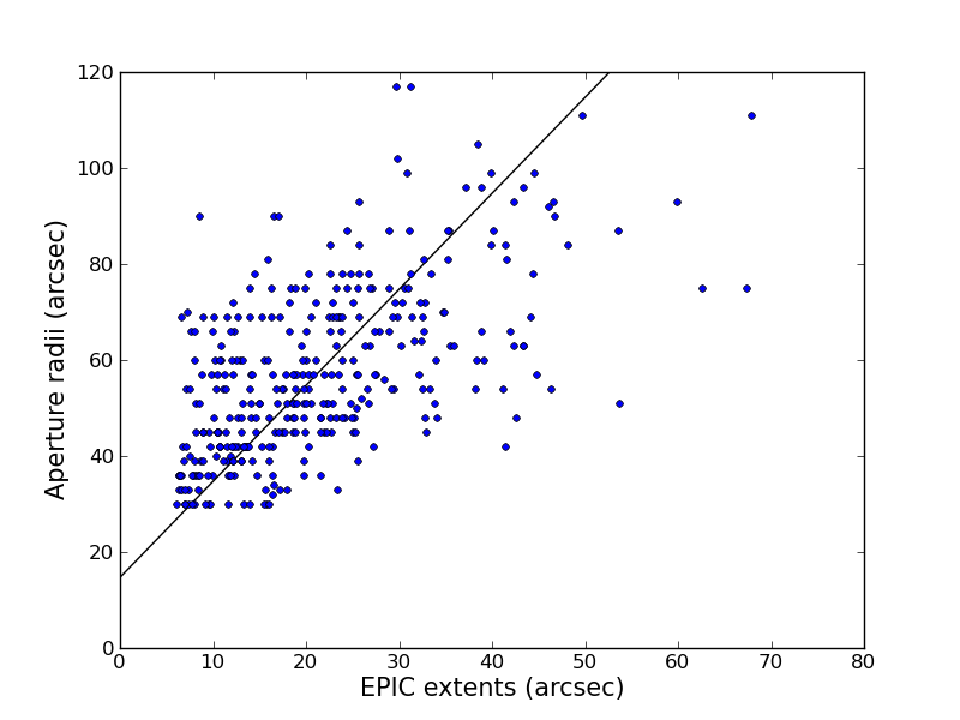
The third input is the aperture bolometric luminosity. For the extended cluster sample (44 systems), we only have the X-ray luminosity in [0.5-2.0] keV computed based on the integrated model flux in [0.5-2.0] keV. We also used the linear relation between the aperture bolometric luminosities and luminosities in [0.5-2.0] keV in order to convert the computed band luminosities to aperture bolometric luminosities, see Section 4.2 in Paper II for more information about this conversion. Based on these inputs, the iterative method provided the measurements of , , and for each cluster.
We compared the current measurements of based on the flux given in the 2XMMi-DR3 catalogue and the corresponding luminosities of the common cluster sample (280 systems) in Paper II. Figure 4.12 shows the comparison between the two measurements of . It shows good agreement between the measured values except a few cases (about 4 percent) that are contaminated by point sources. The median value of the ratios of the present measurements to the ones from Paper II is 1.03. Since there is such a good agreement between the measured luminosities from the current work and the previous one, we trust the current procedure to measure the X-ray parameters for the extended cluster sample.

The first data release of the XMM-Newton Cluster Survey (Mehrtens et al., 2012, XCS,) comprises about 500 clusters. Cross-matching the cluster sample with the XCS sample that have redshift and X-ray luminosity measurements within 30 arcsec yields 97 common objects. Among these, 89 clusters are included in the optically confirmed cluster sample from our survey (Paper II). Figure 4.13 shows the comparison of the current measurements and the corresponding ones from the XCS project. The median ratio between the two measurements is 0.94. In Paper II we showed a better agreement of values for the common sample if we constrain the comparison to the parameters derived from the spectral fits. Among the common sample, 29/97 have only photometric redshifts in the XCS sample, therefore our cluster sample provides spectroscopic confirmation for these systems.
The mass range of the cluster sample is M⊙ and luminosity range is erg s-1. Figure 4.14 shows the distributions of as a function of redshift for the extended cluster sample and the common objects in Paper II as well as for 1730 clusters () from MCXC catalogue that was comprised based on published X-ray selected cluster catalogues from ROSAT data (Piffaretti et al., 2011). Due to the sensitivity of XMM-Newton and deeper exposures for some fields the current cluster sample includes low luminosity groups and clusters at each redshift as shown in Figure 4.14.


Since the current X-ray luminosities are comparable with the previous measurements in Paper II, we only present a catalogue of the extended cluster sample (44 systems) listing their optical and X-ray parameters. In addition to this sample we also provide the spectroscopic redshifts and the X-ray properties for 49 clusters among the common sample in paper II that had only photometric redshifts. These two subsample are compiled together in Table 4.1 with a note refers to each subsample.
Table 4.1, available at the Appendix C, lists the first 10 entries of the extended cluster sample (44 objects) from the current work in addition to a subsample (49 systems) that have only photometric redshifts in Paper II and have spectroscopic confirmations in the current work. The X-ray parameters are measured based on the flux given in the 2XMMi-DR3 catalogue. Cols. [1] and [2] report the cluster identification number (detection Id, detid) and its name (IAUNAME), cols. [3] and [4] provide the coordinates of X-ray emission in equinox J2000.0, col. [5] the XMM-Newton observation Id (obsid), col. [6] the cluster spectroscopic redshift, col. [7] the scale at the cluster redshift in kpc/′′, col. [8] the in kpc, cols. [9], and [10] the 2XMMi-DR3 X-ray flux [0.5-2.0] keV and its error in units of erg cm-2 s-1, cols. [11], and [12] the estimated X-ray luminosity [0.5-2.0] keV and its error in units of erg s-1, cols. [13] and [14] the cluster bolometric luminosity and its error in units of erg s-1, cols. [15] and [16] the cluster mass and its error in units of M⊙, col. [17] the objid of the likely BCG in SDSS-DR9, cols. [18] and [19] the BCG coordinates in equinox J2000.0, col. [20] the apparent magnitude mr of the BCG, col. [21] and [22] the weighted average spectroscopic redshift and the number of cluster members within 500 kpc with available spectroscopic redshifts that were used to compute the average redshift, col. [23] and [24] the weighted average photometric redshift and the number of identified cluster member candidates within 500 kpc based on their photometric redshifts, col. [25] the linear separation between the cluster X-ray position and the BCG position, and col. [26] a note indicating the object status, extended refers to a new system detected using the current procedure, and Paper II refers to a previously known system from Paper II with photometric redshift and confirmed spectroscopically in the current work.
4.5 Summary
We present a sample of 324 X-ray selected galaxy groups and clusters associated with at least one Luminous Red Galaxy (LRG) that has a spectroscopic redshift in the SDSS-DR9. The redshifts of the associated LRGs are used to identify the BCGs and the other cluster galaxies with spectroscopic redshifts. The cluster spectroscopic redshift is computed as the weighted average of the available spectroscopic redshifts of the cluster galaxies within 500 kpc. The cluster sample spans a wide redshift range with a median of . Among the cluster sample, 241 are previously known as optically selected galaxy clusters. The measured redshifts are consistent with the available redshifts in the literature. In addition to re-identify and confirm the redshift measurements of 280 clusters among the published cluster sample from our survey, we extend the optically confirmed cluster sample by 44 systems. Among the extended sample, 55 percent are newly discovered groups and clusters and 80 percent are new X-ray detected clusters. The measured redshifts and the X-ray flux given in the 2XMMi-DR3 catalogue are used to determine the X-ray luminosity of the cluster sample. We also derived X-ray-luminosity-based mass of the sample. Comparing the current estimation of the X-ray bolometric luminosity, , with the available ones from Paper II and the XCS project, we found a good agreement between the two measurements. The distribution of X-ray luminosities of our cluster sample and ROSAT clusters with redshifts showed that we detected less luminous groups and clusters at each redshift.
| detid\tablefootmarka | Name\tablefootmarka | ra\tablefootmarka | dec\tablefootmarka | obsid\tablefootmarka | z\tablefootmarkb | scale | \tablefootmarka,c | \tablefootmarkd | \tablefootmarke | \tablefootmarkf | |||||
|---|---|---|---|---|---|---|---|---|---|---|---|---|---|---|---|
| IAUNAME | (deg) | (deg) | kpc/′′ | (kpc) | (keV) | (keV) | (keV) | ||||||||
| (1) | (2) | (3) | (4) | (5) | (6) | (7) | (8) | (9) | (10) | (11) | (12) | (13) | (14) | (15) | (16) |
| 005735 | 2XMM J003840.4+004746 | 9.66841 | 0.79636 | 0203690101 | 0.5549 | 6.44 | 522.21 | 1.44 | 0.18 | 17.83 | 2.19 | 35.42 | 5.05 | 7.42 | 1.56 |
| 007554 | 2XMM J004304.2-092801 | 10.76751 | -9.46695 | 0065140201 | 0.1866 | 3.12 | 594.22 | 6.84 | 1.06 | 6.74 | 1.05 | 20.30 | 3.72 | 7.18 | 1.56 |
| 010986 | 2XMM J005556.9+003806 | 13.98720 | 0.63507 | 0303110401 | 0.2047 | 3.36 | 541.55 | 5.01 | 0.95 | 6.06 | 1.15 | 12.11 | 2.64 | 5.54 | 1.28 |
| 021043 | 2XMM J015558.5+053159 | 28.99394 | 5.53329 | 0153030701 | 0.4499 | 5.76 | 640.92 | 5.82 | 0.85 | 43.44 | 6.37 | 84.97 | 15.25 | 12.11 | 2.54 |
| 021597 | 2XMM J020019.2+001931 | 30.08012 | 0.32553 | 0101640201 | 0.6825 | 7.07 | 643.12 | 4.17 | 0.52 | 85.10 | 10.59 | 213.07 | 37.70 | 16.13 | 3.35 |
| 030746 | 2XMM J023346.9-085054 | 38.44543 | -8.84844 | 0150470601 | 0.2653 | 4.08 | 587.32 | 5.95 | 1.09 | 12.93 | 2.36 | 24.86 | 5.10 | 7.55 | 1.67 |
| 030889 | 2XMM J023458.7-085055 | 38.74463 | -8.84868 | 0150470601 | 0.2590 | 4.01 | 586.22 | 4.15 | 0.53 | 8.54 | 1.09 | 24.02 | 3.31 | 7.45 | 1.56 |
| 089821 | 2XMM J083114.4+523447 | 127.81014 | 52.57993 | 0092800201 | 0.6107 | 6.74 | 470.06 | 0.79 | 0.11 | 12.25 | 1.64 | 22.80 | 3.72 | 5.78 | 1.26 |
| 089885 | 2XMM J083146.1+525056 | 127.94516 | 52.84719 | 0092800201 | 0.5190 | 6.23 | 582.48 | 3.50 | 0.21 | 36.78 | 2.24 | 60.96 | 5.82 | 9.86 | 1.97 |
| 091280 | 2XMM J083926.4+193658 | 129.86017 | 19.61622 | 0101440401 | 0.3742 | 5.16 | 481.60 | 0.93 | 0.13 | 4.50 | 0.62 | 10.74 | 1.48 | 4.71 | 1.03 |
| detid\tablefootmarka | objid\tablefootmarkg | RA\tablefootmarkg | DEC\tablefootmarkg | \tablefootmarkg | \tablefootmarkg | \tablefootmarkg | \tablefootmarkg | \tablefootmarkg | offset\tablefootmarkg | note\tablefootmarkh |
|---|---|---|---|---|---|---|---|---|---|---|
| (BCG) | (deg) | (deg) | (BCG) | (kpc) | ||||||
| (1) | (17) | (18) | (19) | (20) | (21) | (22) | (23) | (24) | (25) | (26) |
| 005735 | 1237663204918428144 | 9.68054 | 0.78241 | 20.047 | 0.5549 | 3 | 0.5127 | 7 | 429.63 | Extended |
| 007554 | 1237652630713860232 | 10.80832 | -9.47863 | 17.213 | 0.1866 | 2 | 0.1794 | 18 | 473.45 | Extended |
| 010986 | 1237663784740388918 | 14.02537 | 0.62659 | 17.537 | 0.2047 | 3 | 0.1951 | 20 | 473.61 | Extended |
| 021043 | 1237678663047250389 | 28.98754 | 5.53072 | 19.553 | 0.4499 | 1 | 0.4258 | 12 | 142.33 | Paper-II |
| 021597 | 1237657071160263439 | 30.08100 | 0.32491 | 20.448 | 0.6825 | 1 | 0.6555 | 3 | 27.36 | Extended |
| 030746 | 1237653500970139807 | 38.44673 | -8.84925 | 17.540 | 0.2653 | 1 | 0.2547 | 17 | 22.30 | Paper-II |
| 030889 | 1237653500970270877 | 38.74547 | -8.84926 | 17.762 | 0.2590 | 2 | 0.2528 | 17 | 14.70 | Paper-II |
| 089821 | 1237651701914141241 | 127.80965 | 52.57912 | 20.467 | 0.6107 | 1 | 0.6465 | 4 | 20.97 | Extended |
| 089885 | 1237651272960967114 | 127.94343 | 52.84937 | 19.251 | 0.5190 | 2 | 0.5165 | 13 | 54.28 | Paper-II |
| 091280 | 1237667107965108712 | 129.86275 | 19.61566 | 18.114 | 0.3742 | 3 | 0.3542 | 15 | 46.34 | Paper-II |
The entire cluster catalogue is available in the Appendix C. \tablefoottextaParameters extracted from the 2XMMi-DR3 catalogue. \tablefoottextbSpectroscopic redshift as given in col. (21). \tablefoottextc2XMMi-DR3 flux, [0.5-2.0] keV, and its errors in units of erg cm-2 s-1. \tablefoottextdComputed X-ray luminosity, [0.5-2.0] keV, and its errors in units of erg s-1. \tablefoottexteX-ray bolometric luminosity, , and its error in units of erg s-1. \tablefoottextfX-ray-luminosity-based mass and its error in units of M⊙. \tablefoottextgParameters obtained from the current detection algorithm in the optical band. \tablefoottexthA note about each system as extended: new cluster from the current algorithm, and paper-II: a cluster in paper II and spectroscopically confirmed from the present procedure.
Chapter 5 IV. The correlation of X-ray and optical properties** * This chapter will be submitted to Astronomy & Astrophysics
Abstract
We present the absolute magnitude and the optical luminosity in the band of the BCGs of the optically identified cluster sample (574 systems) from the 2XMMi/SDSS Galaxy Cluster Survey. The cluster sample spans a wide redshift range 0.03-0.77 (median =0.33). The correlation between the absolute magnitudes of the BCGs and the cluster redshifts is investigated. We also present the relation between the optical luminosity of the BCG and the cluster mass. For a subsample of 214 systems below a redshift of 0.42 with measured X-ray spectroscopic temperatures, we determined the optical richness and luminosity within . We found a tight relation between the cluster richness and optical luminosity. This subsample is used to perform a comparison of the appearance of galaxy clusters in the X-ray and optical bands. The X-ray parameters and the masses at the radius are obtained from the published cluster catalogue from our survey. We investigate the correlation between the X-ray properties (temperature , luminosity , and X-ray-luminosity-based mass ) and optical properties (richness and luminosity). The relation between the cluster richness and , , and has an orthogonal scatter of 41, 51, and 41, respectively while the relation between the optical luminosity and the same properties has an orthogonal scatter of 38, 48, 38, respectively.
5.1 Introduction
Galaxy clusters are the largest clearly defined objects in the universe. Their baryonic matter has two components: first, the individual galaxies that can be studied through optical or infrared imaging and spectroscopy; the second, a hot diffuse intracluster medium (ICM) that can be observed with X-ray and microwave instruments. Clusters of galaxies are ideal laboratories to study the cosmic evolution of the ICM and the cluster galaxy population. Precise observations of large cluster samples provide a powerful tool to constrain the cosmological parameters (Sarazin, 1988; Rosati et al., 2002; Voit, 2005; Böhringer & Werner, 2010; Allen et al., 2011, e.g.).
Solid observational evidence indicates a strong interaction between the two baryonic components of galaxy clusters. The evolution of galaxies in clusters is influenced by the hot diffuse gas in the ICM. The observed metal abundance in the ICM is produced by the pollution metals expelled from galaxies via galactic winds (Finoguenov et al., 2001; De Grandi & Molendi, 2002). To understand the complex physics of galaxy cluster baryon components, it is required to combine X-ray and optical observations of a large sample of these systems (Popesso et al., 2004).
Several cluster surveys have been conducted in optical/IR wavelengths (Abell, 1958; Abell et al., 1989; Zwicky et al., 1961; Gladders & Yee, 2005; Merchán & Zandivarez, 2005; Koester et al., 2007; Wen et al., 2009; Hao et al., 2010; Szabo et al., 2011; Geach et al., 2011; Durret et al., 2011; Wen et al., 2012; Gettings et al., 2012, e.g.) or in X-rays based on data from previous missions mainly from ROSAT (Ebeling et al., 1998; Böhringer et al., 2004; Reiprich & Böhringer, 2002; Ebeling et al., 2010; Rosati et al., 1998; Burenin et al., 2007, e.g.) or using the current X-ray telescopes (XMM-Newton, Chandra, Swift/X-ray) (Finoguenov et al., 2007; Finoguenov et al., 2010; Adami et al., 2011; Šuhada et al., 2012; Barkhouse et al., 2006; Kolokotronis et al., 2006; Fassbender et al., 2011; Takey et al., 2011; Mehrtens et al., 2012; Clerc et al., 2012; Tundo et al., 2012; de Hoon et al., 2013; Takey et al., 2013a; Takey et al., 2013b, e.g.). So far, tens of thousands clusters have been optically detected while only a few thousands of clusters have been identified in X-rays.
We have initiated a serendipitous search for galaxy clusters in XMM-Newton observation fields that are located in the footprint of the Sloan Digital Sky Survey, SDSS-DR7. The main aim of the survey is to construct a large catalogue of newly discovered X-ray selected groups and clusters up to high redshifts in order to investigate the X-ray scaling relations as well as X-ray-optical relations. Recently, we have published the optically confirmed cluster sample that comprises 530 galaxy groups and clusters from our survey based on the SDSS-DR8 (Takey et al., 2013a). In addition, we have extended the optically confirmed cluster sample by 44 objects based on the recent SDSS-DR9 (Takey et al., 2013b). The published catalogues provide the optical redshift as well as the X-ray luminosity and X-ray luminosity-based mass for all systems. The X-ray data allowed to measure the X-ray temperatures for 60 percent of the sample. The published cluster sample with X-ray temperature measurements, which spans a wide redshift range up to 0.7, was used to investigate the X-ray luminosity-temperature relation (Takey et al., 2013a).
In the present paper, we investigate the correlation between the cluster X-ray and the optical parameters that have been determined in a homogenous way based on the current optically identified cluster sample from our survey. Firstly, we investigate the correlations between the BCG properties (absolute magnitude and optical luminosity) and the cluster global properties (redshift and mass). Secondly, we compute the richness and the optical luminosity within (the radius at which the cluster mean density is 500 times the critical density of the universe) of a nearby subsample (, with a complete membership detection from the SDSS data) with measured X-ray temperatures from our published catalogue. The relation between the estimated optical luminosity and richness is also presented. Finally, the correlation between the cluster optical properties (richness and luminosity) and the cluster global properties (X-ray temperature, luminosity, mass) are investigated.
Several studies have presented the correlations between the X-ray observables such as luminosity and temperature as well as the cluster mass with both optical richness and luminosity (Popesso et al., 2004; Popesso et al., 2005; Lopes et al., 2006; Rykoff et al., 2008; Lopes et al., 2009; Wen et al., 2009; Szabo et al., 2011, e.g.) based on known massive X-ray galaxy clusters in the literature apart from RASS-SDSS sample that comprised galaxy groups and clusters compiled by Popesso et al. (2004). These correlations show the ability to predict the X-ray properties of galaxy clusters, the most expensive to observe, and the cluster mass, the most important parameter for the cosmological studies, from the optical properties, and vice versa within a certain accuracy. These predictions are important for future galaxy cluster surveys conducted only in only one band of the electromagnetic spectrum. Here we investigate these correlations based on our large cluster sample including the newly discovered X-ray groups and clusters from the survey, which are in low and intermediate mass regime.
The presentation of the paper is as the follows. In Section 2, we describe the cluster sample and their X-ray properties. In Section 3, we present the properties of the BCGs against the cluster properties. The strategy to compute the richness and optical luminosity as well as their correlations with X-ray properties and masses are presented in Section 4. We summarise our results in Section 5. The cosmological parameters , and km s-1 Mpc-1 were used throughout this paper.
5.2 The study sample and their X-ray properties
The 2XMMi/SDSS Galaxy Cluster Survey as well as the so far optically confirmed cluster sample are presented in Takey et al. (2011); Takey et al. (2013a); Takey et al. (2013b). Here we present a brief summary about the full optically confirmed cluster sample from the survey, which is used in the present work.
The survey comprises 1180 X-ray cluster candidates selected from the second XMM-Newton serendipitous source catalogue (2XMMi-DR3), which are in the footprint of the SDSS-DR7 that was available at the initiating of our survey. The total overlap area of the XMM-Newton fields at high galactic latitudes, , in the sky coverage by the SDSS-DR7 is 210 deg2. To measure the X-ray properties of these candidates, their redshifts need to be determined. The X-ray data quality of these candidates do not permit to measure their redshifts from the emission lines in the X-ray spectrum apart from very bright X-ray sources (about 4 percent with more than 2000 photon counts). Therefore, the main resource to measure their redshifts is the optical data. The so far largest optical survey is the SDSS, which covers a sky area of 14,555 deg2 and provides positions, magnitudes, and photometric redshifts of galaxies, in addition to spectroscopic redshifts for about one and half millions galaxies (Ahn et al., 2012).
Based on the photometric redshifts of galaxies in the SDSS-DR8, we have optically identified the counterparts of 530 galaxy groups/clusters (Takey et al., 2013a). Then we constructed a cluster sample of 324 systems with spectroscopic confirmations based on the available spectroscopic redshifts of the Luminous Red Galaxies (LRGs) in the SDSS-DR9 (Takey et al., 2013b). The spectroscopic confirmed cluster sample extends the optically confirmed cluster sample by 44 objects and provides spectroscopic confirmations for 49 systems. Therefore, the full cluster list with optical counterparts and redshift measurements comprises 574 galaxy groups/clusters. This is the so far largest X-ray selected galaxy clusters catalogue based on XMM-Newton observations.
The redshifts of the cluster sample span a wide range from 0.03 to 0.77 with a median of 0.33. The distribution of the redshifts of the cluster sample is shown in Figure 5.1. Among the confirmed cluster sample, 70 percent have spectroscopic redshifts for at least one cluster galaxy. About 40 percent of the cluster sample are newly discovered systems as galaxy clusters, while more than 70 percent are new X-ray detections of clusters.
For each system in the sample, we have derived the X-ray bolometric luminosity, , based on the measured luminosity from the spectral fits or based on the flux given in the 2XMMi-DR3 catalogue and the measured redshift. The distribution of the measured luminosities of the cluster sample as well as for identified clusters from ROSAT data (Piffaretti et al., 2011) as a function of redshift is shown in Figure 5.2. The distribution shows that our X-ray detected groups and clusters are in the low and intermediate luminosity regime apart from few luminous systems, thanks to the XMM-Newton sensitivity and the available XMM-Newton deep fields. The measured luminosities are used to measure the cluster mass, , based on the published relation by Pratt et al. (2009). The mass range of the cluster sample is M⊙. For a sub-sample of 345 systems with good X-ray data quality, we measured their X-ray spectroscopic temperatures within an aperture with a radius chosen to optimize the signal-to-noise ratio. The measured temperatures ranges from 0.5 keV to 7.5 keV (Takey et al., 2013a; Takey et al., 2013b).
In the current study, we use the whole optically confirmed sample to investigate the relation between the absolute magnitude of the BCGs and the cluster redshift as well as the relation between the BCG luminosity in band and the cluster mass, see the following section. The systems at redshift below 0.42 with X-ray spectroscopic temperatures are used to investigate the correlation between the optical properties (richness and total luminosity) and the X-ray properties (temperature, luminosity, mass), see Section 4.


5.3 Correlations of the BCG and cluster properties
To determine the optical properties of the cluster sample, we created a galaxy sample from the SDSS-DR9 for each object by selecting the surrounding galaxies within 4 Mpc from the X-ray source position. The galaxies were selected from the Galaxy view table, which contains the photometric parameters measured for resolved primary objects, classified as galaxies. Also, the photometric redshifts and, if available, the spectroscopic redshifts of the galaxy sample were obtained from the Photoz and SpecObj tables, respectively. The extracted parameters of the galaxy sample include the coordinates, the apparent dereddened (model and composite model) magnitudes, K-correction, the photometric redshifts, and, if available, the spectroscopic redshifts. When the spectroscopic redshifts of galaxies are available, we use them instead of the photometric ones. To clean the galaxy sample from faint objects and from galaxies with large photometric redshift errors, we apply a magnitude cut of mag, mag, and a fractional error cut of the photometric redshift, .
For the whole optically confirmed cluster sample we identify the BCG as the brightest galaxy among the cluster luminous member candidates that are selected within the measured and redshift interval from the cluster redshift of . The luminous member galaxies are selected based on their evolution-corrected absolute magnitude that are brighter than . The strategy for selecting the cluster luminous member galaxies is similar to that used by Wen et al. (2012). For each cluster galaxy, we computed its absolute magnitude in the band, Mr, as the follows :
| (5.1) |
where mr is the dereddened model magnitude of the cluster galaxy. is the K-correction in the band derived from the templates and given in the Photoz table in the SDSS-DR9 catalogue data (Csabai et al., 2003). DL is the luminosity distance that was calculated based on the cluster redshift. Then, we corrected the absolute magnitude for a passive evolution as :
| (5.2) |
where Q = 1.62 represent the evolution of the luminosity in units of magnitude per unit redshift, which means that the galaxy was more luminous in the past (Blanton et al., 2003).
Based on the cluster redshift and the angular separation of the BCG from the X-ray peak, we computed its linear separation. The distribution of the linear separations of the BCGs from the X-ray centroids of the sample is shown in Figure 5.3. About 80 percent of the BCGs reside within 200 kpc from the X-ray positions. This percentage is lower than what we found in our published catalogue (90 percent). This is due to selecting the BCG in the previous work as brightest galaxy among the cluster member candidates within one arcmin from the X-ray peak. The systems with large offset of the BCGs might have an ongoing merger or are dynamically active clusters (Rykoff et al., 2008).

The BCGs are in general elliptical massive galaxies and tend to be luminous red galaxies (LRGs) (Postman & Lauer, 1995; Eisenstein et al., 2001; Wen et al., 2012, e.g.). We compared the BCGs magnitudes and colours with the magnitude and colour cuts of the spectroscopically targeted LRGs in the SDSS-III project, BOSS survey†† † http://www.sdss3.org/dr9/algorithms/boss_galaxy_ts.php, (Padmanabhan et al. 2013, in preparation). We found 74 percent of the BCGs satisfy the LRGs criteria in the BOSS survey. Wen et al. (2012) constructed a catalogue of 132,684 clusters based on the photometric redshift of galaxies in the SDSS-DR8. They found 66 percent of the BCGs in their cluster sample fulfill the colour cuts of the SDSS LRG selection criteria.
Several studies (De Lucia & Blaizot, 2007; Stott et al., 2008, e.g.) showed that the BCGs were formed at high redshift, , and have been passively evolving to the present day. The stellar population of the BCGs becomes old with cosmic time and consequently the BCGs become fainter at low redshifts. For each BCG we computed its absolute magnitude in the band, M using Eq. 1. Figure 5.4 shows the relation between M and the cluster redshift, . It shows a weak relation indicating the higher redshift of the cluster, the brighter the BCG is.
We derived the best-fit-linear relation between M and using the BCES regression method (Akritas & Bershady, 1996). The BCES algorithm provides several kinds of linear regression. Here we only show the results of BCES(YX) fitting method, which minimises the residuals in Y, and the BCES orthogonal fitting method, which minimises the squared orthogonal distances. The linear relation between M and is shown in Figure 5.4 and given by :
| (5.3) |
The fitted parameters (intercept and slope) derived from both BCES methods are listed in the first row of the upper part of Table 5.1. The best-fit-lines are also plotted in Figure 5.4. The slope derived by the BCES(YX) algorithm, -2.36 0.16, is much steeper than the published one, -1.74 0.03, by Wen et al. (2012) based an optically cluster sample at . This disagreement might be due to our cluster sample includes less massive clusters and extends to higher redshifts than the sample used by Wen et al. (2012). In addition to using a different fitting method in both projects.
To estimate the orthogonal scatter in the relation, we compute the differences between the measured absolute magnitudes and the predicted ones from the best-fit relation (the fit residuals) based on the cluster redshift from Eq. 3. The residuals of the fit and the slope of the relation are used to compute the orthogonal distances from the best-fit line. The standard deviation of these orthogonal distances was considered as the orthogonal scatter in the relation. The scatter error was computed as the standard error of the measured scatter value. The orthogonal scatters derived from the BCES(YX) and the orthogonal routines of the relation are 0.22 0.01 and 0.13 0.01, respectively and are listed in Table 5.1.
Several groups (Lin & Mohr, 2004; Brough et al., 2008; Popesso et al., 2007; Hansen et al., 2009; Mittal et al., 2009, e.g.) investigated the relation between the optical luminosity of the BCGs and the cluster masses. They found a relation with different exponents as . We measured the optical luminosity of the BCGs in band, , of the cluster sample. The absolute magnitude of each BCG was transformed to absolute luminosity in units of solar luminosities as :
| (5.4) |
The solar absolute magnitude, , was transformed from the Johnson-Morgan-Cousins system to the SDSS system using the transformation equations by Jester et al. (2005). The best fit relation between the logarithms of and the mass of the host cluster, , is shown in Figure 5.5 and given by :
| (5.5) |
The slope, intercept, and the orthogonal scatter of the relations derived from both BCES fitting algorithms are listed in Table 5.1. The scatter is computed in a similar way as in relation but in a logarithmic scale since the fit of the relation is performed in log-log scale. Mittal et al. (2009) investigated the relation based on the HIFLUGCS sample that comprises 64 bright clusters () observed with Chandra. They found a slope derived from the BCES bisector linear regression routine of 0.62 0.05, which is consistent with the present slope 0.57 0.03 obtained using BCES(YX). The present slope is much steeper than the ones (around ) published by Lin & Mohr (2004, e.g.); Brough et al. (2008, e.g.); Popesso et al. (2007, e.g.); Hansen et al. (2009, e.g.).


5.4 Correlations of the cluster X-ray and optical properties
We present the performance of the cluster richness and optical luminosity as predictors of the global X-ray properties (temperature and luminosity) as well as the cluster mass. Popesso et al. (2007) reported that there is no significant difference among the results of the relation between the cluster global properties and the cluster optical luminosity in the different SDSS bands, therefore we will only present the relations for the optical luminosity in the band. Lopes et al. (2009) found that the relations based on parameters extracted within had smaller scatter than the relations based on parameters derived within a fixed radius or within . Therefore we only show here the relations between the X-ray and optical properties that were measured within except the X-ray temperature that was measured within an optimal aperture, which maximises the signal-to-noise ratio.
5.4.1 The cluster richness and optical luminosity
We use a method similar to that described by Wen et al. (2012) to estimate the richness and optical luminosity of the study sample. To estimate the cluster richness, we identify the luminous member candidates within and a redshift interval from the cluster redshift of and with evolution-corrected absolute magnitude . To compute , we first determine the absolute magnitude of each galaxy using Eq. 1, then we correct it for a passive evolution using Eq. 2. The bright end of the cluster member candidates is the absolute magnitude of the BCG, M. The BCG was identified as the brightest galaxy among the cluster luminous galaxies within .
The cluster luminous member galaxies with are complete for clusters up to a redshift of . This is due to the magnitude limit of the SDSS photometric data and the faint limit absolute magnitude used for identifying the luminous member galaxies (Wen et al., 2012). Therefore, we only consider clusters below in investigating the correlation between both the richness and the optical luminosity with the X-ray properties (temperatures, luminosity, and mass). We also include only those clusters with good quality X-ray data that permitted to measure the X-ray temperatures. The subsample includes 214 systems with a temperature range of 0.5-6.8 keV and mass (X-ray-luminosity-based mass) range of M⊙.
The net cluster member galaxies in the region with a radius of after subtraction the expecting foreground and background galaxies is defined as the cluster richness, . To estimate the number of local foreground and background galaxies, we need to count the number of galaxies within a nearby region of the cluster with same redshift and absolute magnitude range of the luminous cluster member candidates. To do this, we divide the annuals between 2-4 Mpc from the X-ray position into 4 sectors. The number of foreground and background galaxies is determined as the mean value of the normalized number of galaxies to region in the 4 sectors within the used redshift and absolute magnitude intervals. We also compute the standard deviations of the galaxy counts in these sectors. If a sector has a number of background galaxies larger than 3 deviation from the mean galaxy count of the 4 sectors, we discard it and re-calculate the mean of galaxy counts in the remaining sectors. This was done in order to avoid any filaments or substructures belonging to the system.
The optical luminosity of a cluster is determined in a similar way as the estimation of the richness. It is computed as the sum of the cluster member luminosities within after subtraction the contamination of the background galaxies luminosity. The luminosity of background galaxies is computed as the mean of the summed optical luminosity of the galaxies with same redshift and absolute magnitude intervals of member galaxies in the 4 sectors. The optical luminosity of the cluster member candidates and the background galaxies are determined for the final galaxy counts resulting from the richness measurements. The absolute magnitude of a galaxy was transformed to absolute luminosity in units of solar luminosities using Eq. 4.
Figure 5.6 shows the relation between the summed band luminosities and richness that were computed within of the subsample below . We found a strong correlation between the measured optical luminosity and the richness. The best linear fits using the BCES regression methods between their logarithms are shown in Figure 5.6 and are expressed by :
| (5.6) |
The slope of the relation is 1.13 0.04 and 0.99 0.03 obtained from the BCES orthogonal and the BCEX(YX) algorithms, respectively. The slopes, intercepts, and orthogonal scatters are given in first raw of the lower part of Table 5.1. The scatter is computed in a similar way as described above and given in a logarithmic scale.
Popesso et al. (2007) investigated the relation between the cluster band optical luminosity within and the net count of cluster galaxies (richness) based on an optically and X-ray selected group and cluster sample of 217 systems at . They found the relation slope is 1.00 0.03 derived from an orthogonal regression method, which is shallower than the present slope 1.13 0.04 (orthogonal) but it is consistent with the slope 0.99 0.03 derived using the BCEX(YX) algorithm. The linear fit derived from the BCES orthogonal method is affected by the two points with large scatter from the best-fit line. Wen et al. (2009) found a slope of 0.97 0.01 between and that were estimated within 1 Mpc from the BCG position for a large optically selected cluster sample at , which is consistent with the present slope 0.99 0.03 derived from the BCEX(YX) algorithm.

5.4.2 The correlation of the cluster richness and optical luminosity with the cluster global properties
The linear relation between the logarithms of the X-ray and optical properties are fitted using the BCES(YX) and orthogonal algorithms and are expressed by :
| (5.7) |
where is the X-ray property (aperture temperature , X-ray luminosity , and X-ray-luminosity-based mass ) and is the optical property (richness and total optical luminosity ). Table 5.1 lists in the lower part the fitting parameters as well as the scatter of each relation. These correlations are shown in Figure 5.7, Figure 5.8, and Figure 5.9. The figures also show the best-fit-lines derived from both BCES(YX) and BCES orthogonal fitting methods.
If we consider the observed relations and (BCES orthogonal) derived from the REXCESS sample that comprises 31 nearby () galaxy clusters (Pratt et al., 2009) and a mass-to-light ratio, (Girardi et al., 2002), we expect a relation between the X-ray temperature and optical luminosity as , a relation between the X-ray and optical luminosity as , and a relation between the cluster mass and optical luminosity as . Since there is a tight relation between the measured optical luminosity and richness with an exponent deviated slightly from the unity as (orthogonal), we expect a slight variation of the exponents of the correlations between the cluster richness and the other cluster properties. The expected relations are , , (orthogonal). Regarding the relations derived from the BCES(YX) algorithm, we expect that the relations between each cluster global parameter with both and have consistent slopes since the slope of relation is approximately the unity, 0.99 0.3, as shown in Table 5.1.
The current slope of the relation, 0.85 0.05 derived from the BCES orthogonal method is consistent with the expected one, 0.83. Popesso et al. (2005) investigated the same relation based on a sample of 49 groups and clusters () with available ASCA temperature. Their optical luminosities were estimated within in the band. They found the slope of the relation obtained using a numerical orthogonal distance regression method is 0.59 0.03, which is much shallower than the present slope 0.85 0.05. This difference in the slope might be introduced from the cluster sample since their sample is small and contained systems with high temperatures apart from few objects (12 systems) with keV, in addition to the different procedures used in estimating the optical luminosities and different aperture used in measuring the temperatures. It is the same case when comparing our relation with the relation published by Lopes et al. (2009) who investigated it based on a small sample of 21 clusters at with keV obtained from the X-Ray Galaxy Clusters Database (BAX).
Wen et al. (2009) found a slope of 0.83 0.08 derived from a cluster sample of 67 systems with ASCA temperature. However, they estimated the optical luminosity within a fixed radius of 1 Mpc and used another fitting method, there is good agreement between the two slopes. The BCES(YX) gives a shallower slope 0.61 0.04 than the one derived from the orthogonal algorithm. The expected relation (orthogonal) is consistent with the derived one based on our cluster sample (orthogonal). Again we found disagreement between the present slope and the published one 0.5 0.07 (orthogonal) by Lopes et al. (2009) due to the differences in the size and mass regime between the two samples. The present slope 0.59 0.06 (BCES(YX)) agrees with the one, 0.61 0.05, published by Wen et al. (2012) who estimated the richness within .
The observed relation, (orthogonal), is in good agreement with the expected one, (orthogonal), from the scaling relations. Popesso et al. (2005) investigated the relation based on a sample of 69 clusters with optical mass, a sample of 49 clusters with mass estimated from the temperature with an overlap of 16 clusters, and the combined sample of 102 systems at , they found the slopes derived from the orthogonal algorithm are 1.59 0.10, 1.89 0.11, and 1.79 0.10, respectively. Lopes et al. (2009) found a slope of 1.62 0.11 derived from a sample of 104 clusters at . The X-ray luminosities in their works were obtained from ROSAT data and were not estimated within a fixed aperture but were calculated from the X-ray luminosity profile. Their optical luminosities were estimated within based on the SDSS data. Once again the present slope is not consistent with the ones derived in those studies due to using different procedure to estimate the X-ray and optical luminosities in addition to the different luminosity regime of the samples.
The present slope 2.71 0.17 of relation agrees well with the published one 2.67 0.12 by Wen et al. (2009) based on a sample of 146 clusters at . The BCES(YX) slope, 1.53 0.11, is shallower than the slope obtained by the BCES orthogonal algorithm. We note that the BCES(YX) slope is consistent with the slopes (orthogonal) published by Popesso et al. (2005); Lopes et al. (2009). Regarding the X-ray luminosity-richness relation, the present exponent is consistent within 1.2 with the expected one (orthogonal) and it is higher than the observed one, 2.79 0.13, by Wen et al. (2009). Lopes et al. (2009) found much shallower slope 1.64 0.10 (orthogonal) than the present one and this might be due to the same reasons mentioned above. The BCES(YX) slope, 1.50 0.14, is consistent with the published one, 1.64 0.10 (orthogonal), by Lopes et al. (2009).
The current slope of relation, 0.97 0.07 (orthogonal), is shallower than the expected one, 1.33 0.12, from the scaling relations. Popesso et al. (2005) investigated the same relation based on the three samples mentioned above and they found slopes (orthogonal) of 1.25 0.06, 0.93 0.06, 1.09 0.04, respectively. Similarly, Lopes et al. (2009) found slopes of 1.09 0.07, 0.99 0.10, and 1.06 0.04 derived from an optically selected sample of 127 systems, X-ray selected sample of 53 clusters, and the combined sample of 180 clusters at , respectively. The two parameters (mass and the optical luminosity in the band) were estimated within in these investigations as our measurements. The current slope is consistent with the slope values from those studies. The BCES(YX) provides a shallower slope of 0.70 0.05.
Regarding relation, we found a relation of (orthogonal) that is shallower than the expected one, (orthogonal). Lopes et al. (2009) found the slope (orthogonal) of the relation derived from the three samples mentioned above are 1.01 0.07, 0.95 0.09, 1.04 0.04, respectively. Their richness and mass were estimated within . The later value is consistent within 1.2 from the present slope. The slope derived from the BCES(YX) method 0.71 0.06 is shallower than the one derived from the BCES orthogonal regression method.
The orthogonal scatter (in a logarithmic scale) of these relations was computed in a similar way as mentioned in the previous section. We note that the BCES orthogonal algorithm provides smaller scatter than the one derived using the BCES(YX) routine. Using the same fitting algorithm, we found the relation between the cluster properties and the optical luminosity have slightly smaller scatter than the relations with the cluster richness. This means that the cluster optical luminosity correlates slightly better than the richness with the cluster global properties (, , and ).
The cluster richness and optical luminosity show a correlation with the cluster X-ray temperature, luminosity and mass. The relation between the cluster richness and , , and has an orthogonal scatter of 41, 51, and 41, respectively while the relation between the optical luminosity and the same properties has an orthogonal scatter of 38, 48, 38, respectively.
The most important parameter of galaxy clusters to be used in cosmological studies is the mass. We showed that the cluster mass can be estimated using a very cheap estimator (richness or optical luminosity) that can be determined from ground-based photometric data. The optical luminosity correlates with the cluster mass with an orthogonal scatter of 38. Popesso et al. (2005) showed that the optical luminosity correlates with the cluster mass much better than the X-ray luminosity. They found an orthogonal scatter in the range 20-30 of relation and an orthogonal scatter 38-50 of relation. Here we found a slightly higher scatter 38 of relation and this is due to including many galaxy groups among our sample, which are the main source of the scatter (Popesso et al., 2004).


5.5 Summary
We re-identified the BCGs of the optically confirmed cluster sample (574 systems) from the 2XMMi/SDSS galaxy cluster survey as the brightest galaxy among the luminous cluster member galaxies within . We found that about 74 percent of the identified BCGs are fulfill the magnitude and colour cuts of the spectroscopically targeted LRGs in the SDSS-III’BOSS. For each BCG, we determined its absolute magnitude and optical luminosity in the band based on the cluster redshift and the SDSS photometric data. We presented the relation between the absolute magnitude of the BCGs with the cluster redshift. The relation between the optical luminosity of the BCGs with the cluster mass was investigated, which shows that the massive clusters have luminous BCGs. We determined the net count of the luminous cluster member galaxies, richness, and their summed luminosity in the band, cluster optical luminosity, within , of 214 galaxy groups and clusters in the redshift range of 0.03-0.42 with available X-ray temperatures from our survey. This subsample comprises systems in low and intermediate mass regime. The estimated optical luminosity is tightly correlated with the cluster richness. We investigated the correlations of the X-ray temperature, luminosity, and the cluster mass with both the optical richness and luminosity of this subsample. The orthogonal scatter in these relations was measured, which indicates that the optical luminosity correlates slightly better than the richness with the cluster global properties. The relation between the cluster richness and , , and has an orthogonal scatter of 41, 51, and 41, respectively while the relation between the optical luminosity and the same properties has an orthogonal scatter of 38, 48, 38, respectively.
| BCES(YX) | Orthogonal | published | |||||||
| relation | a | b | scatter\tablefootmark⋆ | a | b | scatter\tablefootmark⋆ | b | ref. | |
| BCGs | Mr,BCG - z | -22.48 0.05 | -2.36 0.16 | 0.22 0.01 | -20.63 0.18 | -8.13 0.55 | 0.13 0.01 | -1.74 0.03 | 1 |
| Lr,BCG - M500 | 0.70 0.03 | 0.57 0.03 | 0.19 0.01 | 0.37 0.05 | 0.98 0.06 | 0.18 0.01 | 0.62 0.05 | 2 | |
| ClGs | Lr - R | 0.69 0.04 | 0.99 0.03 | 0.09 0.01 | 0.56 0.04 | 1.13 0.04 | 0.08 0.01 | 1.28 0.31 | 3 |
| Tap - R | -0.25 0.06 | 0.59 0.06 | 0.16 0.01 | -0.63 0.08 | 1.00 0.09 | 0.15 0.01 | 0.61 0.05 | 1 | |
| Tap - Lr | -0.68 0.08 | 0.61 0.04 | 0.15 0.01 | -1.07 0.09 | 0.85 0.05 | 0.14 0.01 | 0.59 0.03 | 4 | |
| L500 - R | -0.11 0.13 | 1.50 0.14 | 0.24 0.02 | -1.89 0.23 | 3.43 0.25 | 0.18 0.01 | 1.59 0.09 | 1 | |
| L500 - Lr | -1.18 0.18 | 1.53 0.11 | 0.22 0.01 | -3.07 0.28 | 2.71 0.17 | 0.17 0.01 | 2.67 0.12 | 5 | |
| M500 - R | 0.17 0.06 | 0.71 0.06 | 0.16 0.01 | -0.24 0.08 | 1.15 0.09 | 0.15 0.01 | 1.04 0.04 | 6 | |
| M500 - Lr | -0.30 0.08 | 0.70 0.05 | 0.15 0.01 | -0.74 0.11 | 0.97 0.07 | 0.14 0.01 | 0.99 0.10 | 6 |
⋆The scatter in all relations is the orthogonal scatter in logarithmic scale except the relation that has the scatter in linear scale. \tablebib 1- Wen et al. (2012) ; 2- Mittal et al. (2009) ; 3- Popesso et al. (2007); 4- Popesso et al. (2005); 5- Wen et al. (2009); 6- Lopes et al. (2009).
Chapter 6 Summary, Conclusions, and Outlook
6.1 Summary and Conclusions
In this thesis I have conducted a serendipitous search for galaxy clusters based on the largest X-ray serendipitous source catalogue, 2XMMi-DR3, and the largest optical survey, SDSS. The aims of my survey are to identify new X-ray detected clusters, to trace the evolution of their X-ray scaling relations, and to investigate the correlations between their X-ray and the optical properties. The X-ray cluster candidates are selected among the extended X-ray sources in the 2XMMi-DR3 catalogue. To study the properties of these cluster candidates, the redshifts need to be determined. Therefore, the survey is constrained to those candidates that are in the footprint of the SDSS-DR7 in order to measure their optical redshifts. However, the X-ray spectroscopy provides a tool to measure the X-ray redshift, unfortunately it is only possible for very bright X-ray sources (about 4 percent of the cluster candidates list). Optical redshifts can be obtained from the literature (Takey et al., 2011), using the photometric redshift of the cluster galaxies (Takey et al., 2013a), or using the spectroscopic redshift of the cluster luminous red galaxies (LRGs) from the SDSS data base (Takey et al., 2013b). The optically confirmed cluster sample with redshift measurements can be used to investigates various scaling relations e.g. the X-ray luminosity-temperature relation (Takey et al., 2011; Takey et al., 2013a), relations between the BCG and the cluster properties as well as the correlations between the X-ray and optical properties of the clusters (Takey et al., 2013c). The summary of the main contributions from the thesis work is as the follows:
- 1.
In Chapter 2 I described the 2XMMi/SDSS Galaxy Cluster Survey. The X-ray cluster candidates are selected from extended sources classified as reliable detections (with no warning about being spurious) in the 2XMMi-DR3 catalogue (Watson et al., 2009) at high galactic latitudes, . The overlap area between the XMM-Newton fields and SDSS imaging is 210 deg2. After excluding possible spurious X-ray detections and low redshift galaxies that appear resolved at X-ray wavelengths through visual inspections of X-ray images and X-ray-optical overlays, the X-ray cluster candidates list comprised 1180 objects with at least 80 net photon counts, of which more than 75 percent are new X-ray discoveries. We have demonstrated that the 2XMMi-DR3 catalogue that was based on the archival XMM-Newton data is a rich resource for identifying new X-ray detected clusters (Takey et al., 2011).
- 2.
A quarter of the X-ray cluster candidates had been previously published in optical cluster catalogues based on the SDSS data. Cross-correlations of the X-ray cluster cluster candidates with the recent and largest optical cluster catalogues constructed by Hao et al. (2010); Wen et al. (2009); Koester et al. (2007); Szabo et al. (2011) within a matching radius of one arcmin confirmed 275 clusters and provided us with the photometric redshifts for all of them and the spectroscopic redshifts for 120 BCGs. Based on the cluster redshifts given in those catalogues, we extracted all available spectroscopic redshifts for the cluster members from recent SDSS data (SDSS-DR8). Among the confirmed cluster sample, 182 clusters have spectroscopic redshifts for at least one cluster galaxy. More than 80 percent of the confirmed sample are newly identified X-ray clusters and the others had been previously identified using ROSAT, Chandra, or XMM-Newton data (Takey et al., 2011).
- 3.
I have reduced and analysed the X-ray data of the optically confirmed cluster sample with redshifts from the literature in an automated way following the standard pipelines of processing the XMM-Newton data. In this pipeline, I extracted the cluster spectra from EPIC(PN, MOS1, MOS2) images within an optimal aperture with a radius representing the highest signal-to-noise ratio. The spectral fitting procedure provided the X-ray temperature for 175 systems, which was published as the first cluster sample from our survey. In addition, I derived the physical properties (, and ) of this sample from an iterative procedure using the published scaling relations (Takey et al., 2011).
- 4.
In Chapter 3 I described a finding algorithm developed to detect the optical counterparts of the X-ray cluster candidates and to measure their redshifts using the photometric and, if available, the spectroscopic redshifts of surrounding galaxies from the SDSS-DR8 data. The cluster is recognized if there are at least 8 member galaxies within a radius of 560 kpc from the X-ray emission peak with photometric redshift in the redshift interval of the redshift of the likely identified BCG, . The BCG was identified as the brightest galaxy among those galaxies within one arcmin from the X-ray position that show a peak in the histogram of their photometric redshifts.
The cluster photometric and spectroscopic redshift is measured as the weighted average of the photometric and the available spectroscopic redshifts, respectively, of the cluster galaxies within 560 kpc from the X-ray position. The measured redshifts are in a good agreement with available redshifts in the literature, to date 301 clusters are known as optically selected clusters with redshift measurements. Also, 310 clusters of the optically confirmed cluster sample have spectroscopic redshifts for at least one cluster member galaxy. The measured photometric redshifts are in a good agreement with the measured spectroscopic ones from the survey. The cluster redshifts of the optically confirmed cluster sample span a wide redshift range from 0.03 to 0.70 (Takey et al., 2013a).
- 5.
I reduced and analysed the X-ray data of this sample in a similar way as described above. We presented a cluster catalogue from the survey comprising 345 X-ray selected groups and clusters with their X-ray parameters derived from the spectral fits including the published sample by Takey et al. (2011). In addition to the cluster sample with X-ray spectroscopic data, we presented the remainder of the optically confirmed cluster sample with their X-ray parameters based on the flux given in the 2XMMi-DR3 catalogue. We used the 2XMMi-DR3 flux because of their low quality X-ray data, which is not sufficient to perform spectral fitting. This sample comprises 185 groups and clusters with their fluxes and luminosities in the energy band 0.5-2.0 keV.
For both subsamples, we estimated the physical properties (, and ) from an iterative procedure based on published scaling relations. The measured temperatures and luminosities are in good agreement with published values for the sample overlap (114 systems) with the XMM Cluster Survey (Mehrtens et al., 2012, XCS,). Comparison of the cluster luminosities of the sample with the luminosities of the identified clusters from ROSAT data (Piffaretti et al., 2011) shows that our X-ray detected groups and clusters are in the low and intermediate luminosity regimes apart from few luminous systems, thanks to the XMM-Newton sensitivity and the available XMM-Newton deep fields (Takey et al., 2013a).
- 6.
As a first application of the confirmed cluster sample with measured X-ray temperatures, we investigated the relation for the first time based on a large cluster sample of 345 systems with X-ray spectroscopic parameters drawn from a single survey. The current sample includes groups and clusters with wide ranges of redshifts, temperatures, and luminosities. The slope of the relation is consistent with the published ones of nearby clusters with higher temperatures and luminosities (Pratt et al., 2009; Mittal et al., 2011). The derived relation is still much steeper than that predicted by self-similar evolution (see Chapter 3, Section 3.4.4).
We also investigated the evolution of the slope and the scatter of the relation with the cluster redshift. After excluding the low luminosity groups, we find no significant changes of the slope and the intrinsic scatter of the relation with redshift when dividing the sample into three redshift bins. In addition the slopes of the relations of the three subsamples are in agreement with the corresponding published slopes of the XCS subsamples (Hilton et al., 2012). When including the low luminosity groups in the low redshift subsample, we found its relation becomes flatter than the relation of the intermediate and high redshift subsamples (Takey et al., 2013a).
- 7.
In Chapter 4 I presented a sample of 324 X-ray selected galaxy groups and clusters associated with at least one Luminous Red Galaxy (LRG) that has a spectroscopic redshift in the SDSS-DR9 (Ahn et al., 2012). The redshifts of the associated LRGs are used to identify the BCGs and the other cluster galaxies with spectroscopic redshifts. The cluster spectroscopic redshift is computed as the weighted average of the available spectroscopic redshifts of the cluster galaxies within 500 kpc. The cluster sample spans a wide redshift range from 0.05 to 0.77 with a median redshift of . In addition to re-identify and confirm the redshift measurements of 280 clusters among the published cluster sample from our survey by Takey et al. (2013a), we extended the optically confirmed cluster sample by 44 systems. Among the newly constructed sample, 55 percent are newly discovered systems and 80 percent are new X-ray detected galaxy groups and clusters. The measured redshifts and the X-ray flux given in the 2XMMi-DR3 catalogue were used to determine the X-ray luminosity and mass of the cluster sample (Takey et al., 2013b).
- 8.
In Chapter 5 we investigated the correlations between the optical properties of the BCGs with the cluster properties, as a second application of the optically confirmed cluster sample from our ongoing survey. To check those correlations, I re-identified the BCGs of the whole optically confirmed cluster sample (574 systems) as the brightest galaxy among the luminous cluster member galaxies within . We found that 74 percent of the re-identified BCGs fulfill the magnitude and colour cuts of the spectroscopically targeted LRGs in the BOSS (SDSS-III). For each BCG, we determined its absolute magnitude and optical luminosity in the band. We investigated the relation between the absolute magnitude of the BCGs with the cluster redshift. It shows a linear relation indicating the BCGs are brighter in the high redshift clusters, which is consistent with the result obtained by Wen et al. (2012). The relation between the optical luminosity of the BCGs with the cluster mass was also investigated, which indicated that the more massive the cluster, the more luminous the BCG is. The slope of this relation is consistent with the published one by Mittal et al. (2009) (Takey et al., 2013c).
- 9.
As a third application of the optically confirmed cluster sample, we investigated the correlation between the optical properties (richness and luminosity) and the X-ray properties (temperature, luminosity, mass). To investigate these relations, we determined the net luminous cluster member galaxies within , richness, and their summed luminosity in the band, cluster optical luminosity, of 214 galaxy groups and clusters in the redshift range of 0.03-0.42 with available X-ray temperatures from our survey. This subsample comprises systems in low and intermediate mass regime. The estimated optical luminosity is tightly correlated with the cluster richness.
We investigated the correlations of the X-ray temperature, luminosity, and the cluster mass with both the optical richness and luminosity of this subsample. The orthogonal scatter in these relations was measured. According th the measured scatters, the optical luminosity correlates slightly better than the richness with the cluster global properties. The relation between the cluster richness and , , and has an orthogonal scatter of 41, 51, and 41, respectively, while the relation between the optical luminosity and the same properties has an orthogonal scatter of 38, 48, 38, respectively (Takey et al., 2013c).
- 10.
Finally, the constructed sample from our ongoing survey is the largest X-ray selected cluster catalogue to date based on X-ray data from the current X-ray observatories (XMM-Newton, Chandra, Suzaku, and Swift/XRT). It comprises 574 groups and clusters with their optical and X-ray properties, spanning the redshift range . More than 75 percent of the cluster sample are newly discovered clusters at X-ray wavelengths. About 40 percent of the sample are new systems to the literature according to current entries in the NED (Takey et al., 2013c).
6.2 Future perspectives
I have presented the optically confirmed cluster sample (574 systems) from the 2XMMi/SDSS Galaxy Cluster Survey, which is about half of the X-ray cluster candidates list (1180 objects). In the future I plan to study the remainder of the X-ray cluster candidates, which were not identified by the current detection algorithms since they are either poor or at high redshifts. For the distant clusters, we plan follow-up by imaging and spectroscopy. For those X-ray cluster candidates that have member galaxies detected in the SDSS imaging and not be identified as groups or clusters by the algorithms used in this thesis, I plan to improve these algorithms to constrain their redshifts. By confirming the remainder of the X-ray cluster candidates, especially distant ones, and measuring their redshifts, we will be able to trace the evolution of relation and X-ray-optical relations as well as to asses the selection effects on those relations.
Since the current survey was successful, a natural extension is to continue to enlarge the catalogue of X-ray selected galaxy groups and clusters based on the upcoming version (not yet published) of the XMM-Newton serendipitous source catalogue, 3XMM. The 3XMM catalogue is about 30 percent larger than the 2XMMi-DR3 catalogue. The cluster redshifts will be measured based on the available large optical surveys e.g. the Sloan Digital Sky Survey (SDSS), the Canada-France-Hawaii Telescope Legacy Survey (CHFTLS), the European Southern Observatory (ESO) archive and the Hubble Space Telescope (HST) archive, and Infrared surveys by UKIDSS, the NASA’s Spitzer Space Telescope (SST) and the Wide-field Infrared Survey Explorer (WISE). This extension will be in the frame work of the ARCHES (Astronomical Resource Cross-matching for High Energy Studies) project, which is funded by the 7th Framework of the European Union.
Appendix A Appendix A
Gallery
We present a gallery of four galaxy clusters from the first cluster sample with different X-ray fluxes and data quality at different redshifts covering the whole redshift range of the sample. For each cluster, X-ray flux contours (0.2-4.5 keV) are overlaid on combined image from , , and -SDSS images. The upper panel in each figure shows the X-ray-optical overlays. The field of view is centred on the X-ray cluster position. In each overlay, the cross-hair indicates the position of the brightest cluster galaxy (BCG), while in Figure A.4 the cross-hair indicates the cluster stellar mass centre although it is obvious that the BCG is located at the X-ray emission peak. In each figure, the bottom panel shows the X-ray spectra (EPIC PN (black), MOS1 (green), MOS2 (red)) and the best fitting MEKAL model. The full gallery of the first cluster sample is available at http://www.aip.de/groups/xray/XMM_SDSS_CLUSTERS/17498.html.


Appendix B Appendix B
Selection criteria of LRGs
We used the colour and magnitude cuts that were used to select the spectroscopic targets to construct BOSS galaxy sample in the SDSS-III project. The selection criteria of galaxies targeted in BOSS were given in (Padmanabhan et al. 2013) and were provided in the BOSS homepage ** * http://www.sdss3.org/dr9/algorithms/boss_galaxy_ts.php.
The BOSS includes two samples of galaxies,
(i) The BOSS LOWZ Galaxy Sample,
The selection cuts are as follows:
- 1.
, to define the colour boundaries of the sample around a passive stellar population, where
- 2.
, to select the brightest galaxies at each redshift, where
- 3.
, to define the faint and bright limits
(ii) The BOSS CMASS Galaxy Sample,
The colour and magnitude cuts are as follows:
- 1.
, to isolate high-redshift objects, where
- 2.
, to select the brightest or more massive galaxies with redshift
- 3.
, to define the faint and bright limits
- 4.
, to protect from some outliers
Note that we did not apply the criteria that were used to perform a star-galaxy separation since we dealt only with objects that were classified as galaxies indicated by spectroscopic class parameters given in the SpecObj table. Note also all colours are computed using model magnitudes while the magnitude cuts are applied on composite model (cmodel) magnitudes. All magnitudes are corrected for Galactic extinction following Schlegel et al. (1998).
Appendix C Appendix C
| detid\tablefootmarka | Name\tablefootmarka | ra\tablefootmarka | dec\tablefootmarka | obsid\tablefootmarka | z\tablefootmarkb | scale | \tablefootmarka,c | \tablefootmarkd | \tablefootmarke | \tablefootmarkf | |||||
| IAUNAME | (deg) | (deg) | kpc/′′ | (kpc) | (keV) | (keV) | (keV) | ||||||||
| (1) | (2) | (3) | (4) | (5) | (6) | (7) | (8) | (9) | (10) | (11) | (12) | (13) | (14) | (15) | (16) |
| 005735 | 2XMM J003840.4+004746 | 9.66841 | 0.79636 | 0203690101 | 0.5549 | 6.44 | 522.21 | 1.44 | 0.18 | 17.83 | 2.19 | 35.42 | 5.05 | 7.42 | 1.56 |
| 007554 | 2XMM J004304.2-092801 | 10.76751 | -9.46695 | 0065140201 | 0.1866 | 3.12 | 594.22 | 6.84 | 1.06 | 6.74 | 1.05 | 20.30 | 3.72 | 7.18 | 1.56 |
| 010986 | 2XMM J005556.9+003806 | 13.98720 | 0.63507 | 0303110401 | 0.2047 | 3.36 | 541.55 | 5.01 | 0.95 | 6.06 | 1.15 | 12.11 | 2.64 | 5.54 | 1.28 |
| 021043 | 2XMM J015558.5+053159 | 28.99394 | 5.53329 | 0153030701 | 0.4499 | 5.76 | 640.92 | 5.82 | 0.85 | 43.44 | 6.37 | 84.97 | 15.25 | 12.11 | 2.54 |
| 021597 | 2XMM J020019.2+001931 | 30.08012 | 0.32553 | 0101640201 | 0.6825 | 7.07 | 643.12 | 4.17 | 0.52 | 85.10 | 10.59 | 213.07 | 37.70 | 16.13 | 3.35 |
| 030746 | 2XMM J023346.9-085054 | 38.44543 | -8.84844 | 0150470601 | 0.2653 | 4.08 | 587.32 | 5.95 | 1.09 | 12.93 | 2.36 | 24.86 | 5.10 | 7.55 | 1.67 |
| 030889 | 2XMM J023458.7-085055 | 38.74463 | -8.84868 | 0150470601 | 0.2590 | 4.01 | 586.22 | 4.15 | 0.53 | 8.54 | 1.09 | 24.02 | 3.31 | 7.45 | 1.56 |
| 089821 | 2XMM J083114.4+523447 | 127.81014 | 52.57993 | 0092800201 | 0.6107 | 6.74 | 470.06 | 0.79 | 0.11 | 12.25 | 1.64 | 22.80 | 3.72 | 5.78 | 1.26 |
| 089885 | 2XMM J083146.1+525056 | 127.94516 | 52.84719 | 0092800201 | 0.5190 | 6.23 | 582.48 | 3.50 | 0.21 | 36.78 | 2.24 | 60.96 | 5.82 | 9.86 | 1.97 |
| 091280 | 2XMM J083926.4+193658 | 129.86017 | 19.61622 | 0101440401 | 0.3742 | 5.16 | 481.60 | 0.93 | 0.13 | 4.50 | 0.62 | 10.74 | 1.48 | 4.71 | 1.03 |
| 091629 | 2XMM J084124.2+004640 | 130.35101 | 0.77799 | 0202940201 | 0.4075 | 5.43 | 615.91 | 4.28 | 0.29 | 25.27 | 1.69 | 56.45 | 5.47 | 10.23 | 2.03 |
| 099426 | 2XMM J094034.6+355945 | 145.14429 | 35.99594 | 0021740101 | 0.3011 | 4.47 | 560.28 | 3.01 | 0.41 | 8.75 | 1.19 | 21.08 | 3.39 | 6.82 | 1.46 |
| 099550 | 2XMM J094107.7+032912 | 145.28229 | 3.48674 | 0306050201 | 0.2490 | 3.90 | 443.09 | 0.77 | 0.14 | 1.45 | 0.27 | 4.04 | 0.63 | 3.18 | 0.74 |
| 103306 | 2XMM J095945.4+023634 | 149.93957 | 2.60961 | 0302351601 | 0.3445 | 4.89 | 443.47 | 0.82 | 0.16 | 3.26 | 0.65 | 5.75 | 1.33 | 3.55 | 0.87 |
| 104390 | 2XMM J100056.7+023343 | 150.23611 | 2.56332 | 0203360601 | 0.2194 | 3.54 | 463.19 | 1.53 | 0.26 | 2.16 | 0.37 | 4.80 | 0.77 | 3.52 | 0.81 |
| 104705 | 2XMM J100117.0+021658 | 150.32104 | 2.28282 | 0302350801 | 0.1225 | 2.20 | 398.12 | 0.75 | 0.14 | 0.30 | 0.06 | 1.35 | 0.22 | 2.02 | 0.50 |
| 105537 | 2XMM J100217.2+015625 | 150.57174 | 1.94037 | 0203360401 | 0.3082 | 4.54 | 448.94 | 1.41 | 0.39 | 4.33 | 1.19 | 5.43 | 2.02 | 3.54 | 1.00 |
| 106241 | 2XMM J100423.5+410008 | 151.09813 | 41.00230 | 0207130201 | 0.3583 | 5.02 | 454.11 | 1.02 | 0.28 | 4.46 | 1.24 | 7.01 | 2.42 | 3.87 | 1.05 |
| 106515 | 2XMM J100713.3+124718 | 151.80582 | 12.78839 | 0140550601 | 0.2481 | 3.89 | 422.58 | 0.49 | 0.12 | 0.91 | 0.22 | 3.00 | 0.58 | 2.76 | 0.67 |
| 109295 | 2XMM J102748.7+000336 | 156.95333 | 0.06013 | 0305980401 | 0.7060 | 7.17 | 730.83 | 7.85 | 0.62 | 173.96 | 13.79 | 518.41 | 57.07 | 24.35 | 4.78 |
| 109850 | 2XMM J103003.5+052023 | 157.51499 | 5.33982 | 0148560501 | 0.3082 | 4.54 | 480.19 | 1.49 | 0.14 | 4.56 | 0.42 | 8.26 | 0.95 | 4.33 | 0.95 |
| 109997 | 2XMM J103027.8+310802 | 157.61623 | 31.13392 | 0102040301 | 0.4622 | 5.85 | 510.06 | 1.51 | 0.22 | 12.00 | 1.71 | 21.41 | 3.59 | 6.19 | 1.35 |
| 110111 | 2XMM J103046.8+052751 | 157.69516 | 5.46432 | 0148560501 | 0.3772 | 5.18 | 489.68 | 0.88 | 0.07 | 4.31 | 0.35 | 12.04 | 0.99 | 4.96 | 1.05 |
| 112052 | 2XMM J104104.0+060130 | 160.26679 | 6.02522 | 0151390101 | 0.5056 | 6.14 | 483.60 | 0.85 | 0.11 | 8.34 | 1.12 | 18.13 | 2.86 | 5.55 | 1.21 |
| 118189 | 2XMM J105215.5+441759 | 163.06461 | 44.29999 | 0146990201 | 0.4982 | 6.09 | 535.68 | 1.16 | 0.22 | 11.07 | 2.05 | 33.37 | 6.71 | 7.48 | 1.65 |
| 118353 | 2XMM J105226.8+441859 | 163.11217 | 44.31609 | 0146990201 | 0.4983 | 6.09 | 615.15 | 3.50 | 0.44 | 33.38 | 4.20 | 79.15 | 12.35 | 11.33 | 2.34 |
| 121351 | 2XMM J110344.0+360513 | 165.93374 | 36.08715 | 0205370101 | 0.4972 | 6.09 | 478.28 | 0.84 | 0.13 | 7.93 | 1.24 | 16.38 | 3.11 | 5.32 | 1.20 |
| 121575 | 2XMM J110355.9+360025 | 165.98326 | 36.00699 | 0205370101 | 0.3328 | 4.78 | 427.50 | 0.49 | 0.08 | 1.81 | 0.31 | 4.38 | 0.71 | 3.14 | 0.74 |
| 125233 | 2XMM J111659.0+174953 | 169.24600 | 17.83141 | 0099030101 | 0.4386 | 5.68 | 550.28 | 2.28 | 0.41 | 15.99 | 2.89 | 31.44 | 6.65 | 7.56 | 1.69 |
| 128668 | 2XMM J113804.0+031525 | 174.51687 | 3.25708 | 0111970701 | 0.4491 | 5.75 | 610.45 | 3.59 | 0.52 | 26.66 | 3.84 | 62.51 | 10.34 | 10.45 | 2.18 |
| 132492 | 2XMM J120544.4+352307 | 181.43514 | 35.38554 | 0148742401 | 0.6530 | 6.94 | 553.21 | 1.89 | 0.41 | 34.66 | 7.50 | 74.25 | 19.42 | 9.91 | 2.29 |
| 133193 | 2XMM J120933.9+392234 | 182.39078 | 39.37648 | 0112830201 | 0.5548 | 6.44 | 575.26 | 2.72 | 0.20 | 33.53 | 2.48 | 64.74 | 6.35 | 9.91 | 1.98 |
| 134697 | 2XMM J121205.3+131739 | 183.02238 | 13.29430 | 0112550501 | 0.4489 | 5.75 | 569.61 | 2.88 | 0.31 | 21.41 | 2.34 | 40.55 | 5.22 | 8.49 | 1.75 |
| 135421 | 2XMM J121658.3+065826 | 184.24317 | 6.97416 | 0204650201 | 0.4842 | 6.00 | 615.82 | 3.26 | 0.70 | 28.96 | 6.24 | 75.49 | 19.08 | 11.18 | 2.54 |
| 135555 | 2XMM J121733.6+071035 | 184.39023 | 7.17641 | 0204650201 | 0.5796 | 6.58 | 552.31 | 2.13 | 0.38 | 29.18 | 5.15 | 55.28 | 11.54 | 9.03 | 1.98 |
| 139177 | 2XMM J122643.5+334555 | 186.68155 | 33.76528 | 0200340101 | 0.7664 | 7.40 | 499.09 | 0.91 | 0.09 | 24.59 | 2.36 | 60.66 | 7.14 | 8.34 | 1.71 |
| 140028 | 2XMM J122903.6+015012 | 187.26514 | 1.83680 | 0159960101 | 0.3139 | 4.59 | 475.65 | 1.26 | 0.35 | 4.03 | 1.12 | 7.95 | 2.51 | 4.23 | 1.10 |
| 142993 | 2XMM J123232.4+200350 | 188.13529 | 20.06410 | 0301450201 | 0.0635 | 1.22 | 444.98 | 1.91 | 0.39 | 0.19 | 0.04 | 2.23 | 0.33 | 2.66 | 0.63 |
| 143008 | 2XMM J123235.9+000233 | 188.14990 | 0.04251 | 0203170301 | 0.6832 | 7.08 | 486.42 | 0.86 | 0.07 | 17.68 | 1.44 | 37.40 | 3.26 | 6.99 | 1.43 |
| 147020 | 2XMM J124425.3+164759 | 191.10564 | 16.79993 | 0302581501 | 0.2346 | 3.73 | 505.70 | 1.66 | 0.17 | 2.73 | 0.28 | 8.76 | 0.43 | 4.66 | 0.98 |
| 147115 | 2XMM J124448.8-001949 | 191.20335 | -0.33035 | 0110980201 | 0.4693 | 5.90 | 510.22 | 1.24 | 0.12 | 10.26 | 0.96 | 22.05 | 2.51 | 6.25 | 1.31 |
| 149238 | 2XMM J125313.4+155612 | 193.30610 | 15.93687 | 0082990101 | 0.2754 | 4.19 | 702.73 | 12.17 | 1.19 | 28.83 | 2.82 | 78.97 | 12.24 | 13.07 | 2.68 |
| 158679 | 2XMM J132505.0+302445 | 201.27118 | 30.41268 | 0025740201 | 0.4348 | 5.65 | 635.41 | 4.24 | 0.60 | 29.14 | 4.15 | 76.03 | 12.89 | 11.59 | 2.42 |
| 159400 | 2XMM J132631.5+074503 | 201.63141 | 7.75093 | 0200730201 | 0.5327 | 6.31 | 484.00 | 0.86 | 0.12 | 9.67 | 1.39 | 20.23 | 3.24 | 5.75 | 1.26 |
| 160031 | 2XMM J132905.8+582655 | 202.27296 | 58.44784 | 0142770301 | 0.1566 | 2.71 | 488.76 | 1.48 | 0.27 | 0.99 | 0.18 | 5.42 | 0.63 | 3.87 | 0.86 |
| 160695 | 2XMM J133046.2+334620 | 202.69291 | 33.77228 | 0305361601 | 0.4587 | 5.82 | 515.54 | 1.94 | 0.29 | 15.17 | 2.23 | 22.58 | 4.50 | 6.37 | 1.42 |
| 162382 | 2XMM J133458.4+375019 | 203.74351 | 37.83850 | 0109661001 | 0.3834 | 5.23 | 499.71 | 1.38 | 0.11 | 7.03 | 0.56 | 13.99 | 1.36 | 5.31 | 1.12 |
| 162545 | 2XMM J133514.1+374908 | 203.80896 | 37.81876 | 0109661001 | 0.6965 | 7.13 | 561.72 | 2.07 | 0.12 | 44.47 | 2.67 | 96.69 | 8.08 | 10.93 | 2.15 |
| 163928 | 2XMM J133852.5+044309 | 204.71904 | 4.71926 | 0152940101 | 0.7264 | 7.25 | 593.32 | 3.00 | 0.35 | 71.26 | 8.29 | 152.84 | 23.61 | 13.35 | 2.73 |
| 164535 | 2XMM J134138.7+001721 | 205.41160 | 0.28936 | 0111281001 | 0.5054 | 6.14 | 698.23 | 9.49 | 1.17 | 93.56 | 11.54 | 179.29 | 26.54 | 16.71 | 3.38 |
| 164909 | 2XMM J134304.9-000053 | 205.77057 | -0.01498 | 0202460101 | 0.7151 | 7.21 | 761.31 | 12.50 | 0.44 | 285.99 | 10.01 | 693.11 | 48.62 | 27.83 | 5.37 |
| 165043 | 2XMM J134330.3+403051 | 205.87636 | 40.51441 | 0070340701 | 0.7084 | 7.18 | 501.33 | 0.92 | 0.11 | 20.58 | 2.46 | 49.80 | 6.53 | 7.88 | 1.63 |
| 171595 | 2XMM J141256.9-030918 | 213.23753 | -3.15574 | 0013140101 | 0.6697 | 7.02 | 541.50 | 1.62 | 0.27 | 31.57 | 5.30 | 69.32 | 13.66 | 9.48 | 2.05 |
| 171668 | 2XMM J141313.0-031732 | 213.30419 | -3.29242 | 0013140101 | 0.3088 | 4.54 | 500.87 | 1.54 | 0.31 | 4.74 | 0.96 | 10.77 | 2.20 | 4.91 | 1.13 |
| 173756 | 2XMM J142305.5+382807 | 215.77325 | 38.46869 | 0147570601 | 0.4508 | 5.77 | 550.27 | 1.79 | 0.27 | 13.39 | 2.03 | 32.92 | 4.90 | 7.67 | 1.62 |
| 174085 | 2XMM J142732.7+264122 | 216.88659 | 26.68946 | 0111290601 | 0.2293 | 3.67 | 393.65 | 0.53 | 0.14 | 0.83 | 0.21 | 1.80 | 0.47 | 2.18 | 0.58 |
| 178050 | 2XMM J145317.4+033446 | 223.32278 | 3.57946 | 0150350101 | 0.3710 | 5.13 | 658.33 | 5.52 | 0.28 | 26.11 | 1.33 | 74.58 | 6.87 | 11.97 | 2.35 |
| 178120 | 2XMM J145351.0+032319 | 223.46267 | 3.38865 | 0150350101 | 0.3685 | 5.11 | 509.66 | 1.64 | 0.26 | 7.61 | 1.23 | 14.96 | 2.87 | 5.54 | 1.25 |
| 180311 | 2XMM J150918.8-001424 | 227.32855 | -0.24013 | 0305750201 | 0.2625 | 4.05 | 592.47 | 5.56 | 0.93 | 11.81 | 1.97 | 25.99 | 4.61 | 7.72 | 1.67 |
| 184398 | 2XMM J154931.9+213259 | 237.38303 | 21.54999 | 0136040101 | 0.6357 | 6.86 | 679.01 | 5.08 | 0.31 | 87.20 | 5.29 | 249.36 | 24.50 | 17.95 | 3.50 |
| 185578 | 2XMM J155930.6+350441 | 239.87761 | 35.07807 | 0112600801 | 0.4895 | 6.04 | 557.90 | 2.30 | 0.44 | 21.04 | 3.98 | 41.60 | 9.08 | 8.37 | 1.86 |
| 187930 | 2XMM J161713.8+123805 | 244.30779 | 12.63495 | 0103461001 | 0.1987 | 3.28 | 497.04 | 1.27 | 0.25 | 1.44 | 0.29 | 6.94 | 1.04 | 4.26 | 0.95 |
| 200392 | 2XMM J172335.5+341155 | 260.89826 | 34.19881 | 0102040101 | 0.4428 | 5.71 | 762.32 | 11.78 | 1.79 | 84.63 | 12.89 | 244.14 | 54.38 | 20.21 | 4.39 |
| 262357 | 2XMMI J081129.1+481011 | 122.87145 | 48.17000 | 0402780701 | 0.6075 | 6.72 | 531.93 | 1.53 | 0.31 | 23.53 | 4.75 | 48.71 | 11.43 | 8.34 | 1.89 |
| 264469 | 2XMMI J092623.1+362132 | 141.59634 | 36.35902 | 0402370101 | 0.6558 | 6.96 | 539.87 | 1.81 | 0.17 | 33.56 | 3.19 | 64.46 | 7.79 | 9.24 | 1.88 |
| 264943 | 2XMMI J095610.3-002151 | 149.04328 | -0.36440 | 0206430101 | 0.5828 | 6.59 | 607.25 | 3.60 | 0.32 | 50.02 | 4.45 | 101.16 | 11.49 | 12.06 | 2.40 |
| 265123 | 2XMMI J095801.8+020147 | 149.50756 | 2.02998 | 0302352401 | 0.6740 | 7.04 | 410.88 | 0.65 | 0.65 | 12.96 | 7.78 | 12.59 | 10.50 | 4.16 | 1.89 |
| 274756 | 2XMMI J134549.4+074440 | 206.45601 | 7.74465 | 0405950501 | 0.6573 | 6.96 | 536.03 | 1.48 | 0.27 | 27.48 | 4.95 | 61.99 | 13.51 | 9.06 | 2.01 |
| 275328 | 2XMMI J143713.9+341519 | 219.30818 | 34.25553 | 0405200101 | 0.5426 | 6.37 | 674.95 | 6.93 | 0.77 | 80.95 | 9.05 | 167.42 | 24.46 | 15.78 | 3.19 |
| 275341 | 2XMMI J143742.9+340810 | 219.42892 | 34.13626 | 0405200101 | 0.5446 | 6.38 | 609.39 | 3.44 | 0.44 | 40.58 | 5.21 | 89.20 | 15.36 | 11.64 | 2.43 |
| 278534 | 2XMMI J164729.3+271241 | 251.87220 | 27.21165 | 0304071801 | 0.4937 | 6.06 | 427.28 | 0.57 | 0.22 | 5.33 | 2.09 | 8.00 | 3.85 | 3.78 | 1.19 |
| 287820 | 2XMMI J220605.5-001110 | 331.52310 | -0.18635 | 0401180101 | 0.3878 | 5.27 | 475.32 | 0.89 | 0.18 | 4.68 | 0.94 | 10.41 | 2.19 | 4.59 | 1.07 |
| 309493 | 2XMMI J081058.2+500529 | 122.74276 | 50.09156 | 0401270401 | 0.4029 | 5.40 | 638.50 | 6.08 | 0.45 | 34.94 | 2.57 | 69.46 | 7.11 | 11.33 | 2.25 |
| 309859 | 2XMMI J082432.7+294757 | 126.13630 | 29.79925 | 0504102001 | 0.2094 | 3.42 | 490.66 | 1.06 | 0.18 | 1.35 | 0.23 | 6.65 | 0.73 | 4.14 | 0.91 |
| 310772 | 2XMMI J084052.6+383847 | 130.21920 | 38.64663 | 0502060201 | 0.1171 | 2.12 | 466.97 | 1.64 | 0.15 | 0.58 | 0.05 | 3.58 | 0.13 | 3.24 | 0.72 |
| 311197 | 2XMMI J085253.3+175718 | 133.22230 | 17.95522 | 0305480301 | 0.2076 | 3.40 | 469.72 | 1.02 | 0.09 | 1.28 | 0.12 | 5.03 | 0.14 | 3.63 | 0.79 |
| 312824 | 2XMMI J092209.5+063230 | 140.53973 | 6.54177 | 0502920101 | 0.1720 | 2.93 | 393.26 | 0.79 | 0.21 | 0.65 | 0.17 | 1.47 | 0.38 | 2.05 | 0.55 |
| 315216 | 2XMMI J103007.0-030638 | 157.52957 | -3.11081 | 0404840201 | 0.4394 | 5.68 | 567.31 | 2.75 | 0.18 | 19.42 | 1.26 | 38.13 | 2.85 | 8.29 | 1.66 |
| 315488 | 2XMMI J103421.4+395153 | 158.58926 | 39.86479 | 0506440101 | 0.6043 | 6.71 | 476.15 | 0.75 | 0.15 | 11.37 | 2.32 | 24.10 | 5.37 | 5.96 | 1.37 |
| 317881 | 2XMMI J112712.0+025956 | 171.80019 | 2.99890 | 0551021201 | 0.5388 | 6.35 | 552.50 | 2.54 | 0.59 | 29.21 | 6.81 | 47.31 | 13.61 | 8.62 | 2.07 |
| 318253 | 2XMMI J114541.4+025415 | 176.42267 | 2.90425 | 0551022701 | 0.2799 | 4.24 | 474.30 | 1.05 | 0.16 | 2.58 | 0.40 | 6.90 | 0.82 | 4.04 | 0.89 |
| 318315 | 2XMMI J114619.2+025609 | 176.58015 | 2.93602 | 0551022701 | 0.1584 | 2.74 | 421.56 | 1.00 | 0.27 | 0.69 | 0.18 | 2.17 | 0.46 | 2.49 | 0.62 |
| 319555 | 2XMMI J120045.3+342454 | 180.18887 | 34.41505 | 0551630301 | 0.2627 | 4.05 | 475.86 | 1.22 | 0.15 | 2.60 | 0.32 | 6.62 | 0.63 | 4.00 | 0.88 |
| 320719 | 2XMMI J121921.0+060134 | 184.83777 | 6.02628 | 0502120101 | 0.3535 | 4.97 | 438.54 | 0.72 | 0.17 | 3.06 | 0.71 | 5.54 | 1.45 | 3.47 | 0.87 |
| 321268 | 2XMM J123050.8+413415 | 187.71095 | 41.57120 | 0556300101 | 0.7455 | 7.32 | 509.26 | 1.11 | 0.15 | 28.22 | 3.68 | 63.43 | 9.38 | 8.64 | 1.80 |
| 322726 | 2XMMI J124919.4+051837 | 192.33104 | 5.31033 | 0503610101 | 0.4200 | 5.53 | 489.75 | 1.18 | 0.16 | 7.46 | 1.00 | 14.16 | 2.42 | 5.22 | 1.16 |
| 322873 | 2XMMI J125003.9+052118 | 192.51654 | 5.35501 | 0503610101 | 0.3849 | 5.25 | 444.65 | 0.83 | 0.11 | 4.27 | 0.58 | 6.79 | 1.21 | 3.75 | 0.87 |
| 325696 | 2XMMI J133805.9-013501 | 204.52478 | -1.58373 | 0502060101 | 0.3481 | 4.92 | 614.91 | 3.33 | 0.44 | 13.55 | 1.79 | 44.75 | 6.65 | 9.50 | 1.97 |
| 327024 | 2XMMI J142114.9+030745 | 215.31213 | 3.12938 | 0502480701 | 0.3122 | 4.58 | 638.61 | 6.90 | 0.61 | 21.82 | 1.92 | 49.66 | 5.66 | 10.22 | 2.06 |
| 327387 | 2XMMI J143113.8-000618 | 217.80765 | -0.10501 | 0501540201 | 0.7122 | 7.19 | 533.53 | 1.71 | 0.31 | 38.72 | 7.09 | 74.55 | 16.73 | 9.54 | 2.12 |
| 327608 | 2XMMI J143927.3+001249 | 219.86378 | 0.21364 | 0551200101 | 0.3000 | 4.45 | 464.71 | 0.96 | 0.15 | 2.77 | 0.44 | 6.54 | 0.95 | 3.89 | 0.88 |
| 329022 | 2XMMI J145709.1-010057 | 224.28792 | -1.01585 | 0502780601 | 0.2742 | 4.18 | 606.21 | 2.98 | 0.30 | 6.99 | 0.71 | 31.27 | 4.44 | 8.38 | 1.74 |
| 331167 | 2XMMI J151529.5+003943 | 228.87305 | 0.66205 | 0556210501 | 0.2645 | 4.07 | 616.16 | 3.47 | 0.39 | 7.50 | 0.85 | 33.44 | 5.15 | 8.71 | 1.82 |
| detid\tablefootmarka | objid\tablefootmarkg | RA\tablefootmarkg | DEC\tablefootmarkg | \tablefootmarkg | \tablefootmarkg | \tablefootmarkg | \tablefootmarkg | \tablefootmarkg | offset\tablefootmarkg | note\tablefootmarkh |
| (BCG) | (deg) | (deg) | (BCG) | (kpc) | ||||||
| (1) | (17) | (18) | (19) | (20) | (21) | (22) | (23) | (24) | (25) | (26) |
| 005735 | 1237663204918428144 | 9.68054 | 0.78241 | 20.047 | 0.5549 | 3 | 0.5127 | 7 | 429.63 | Extended |
| 007554 | 1237652630713860232 | 10.80832 | -9.47863 | 17.213 | 0.1866 | 2 | 0.1794 | 18 | 473.45 | Extended |
| 010986 | 1237663784740388918 | 14.02537 | 0.62659 | 17.537 | 0.2047 | 3 | 0.1951 | 20 | 473.61 | Extended |
| 021043 | 1237678663047250389 | 28.98754 | 5.53072 | 19.553 | 0.4499 | 1 | 0.4258 | 12 | 142.33 | Paper-II |
| 021597 | 1237657071160263439 | 30.08100 | 0.32491 | 20.448 | 0.6825 | 1 | 0.6555 | 3 | 27.36 | Extended |
| 030746 | 1237653500970139807 | 38.44673 | -8.84925 | 17.540 | 0.2653 | 1 | 0.2547 | 17 | 22.30 | Paper-II |
| 030889 | 1237653500970270877 | 38.74547 | -8.84926 | 17.762 | 0.2590 | 2 | 0.2528 | 17 | 14.70 | Paper-II |
| 089821 | 1237651701914141241 | 127.80965 | 52.57912 | 20.467 | 0.6107 | 1 | 0.6465 | 4 | 20.97 | Extended |
| 089885 | 1237651272960967114 | 127.94343 | 52.84937 | 19.251 | 0.5190 | 2 | 0.5165 | 13 | 54.28 | Paper-II |
| 091280 | 1237667107965108712 | 129.86275 | 19.61566 | 18.114 | 0.3742 | 3 | 0.3542 | 15 | 46.34 | Paper-II |
| 091629 | 1237648722282742639 | 130.35096 | 0.77637 | 19.415 | 0.4075 | 1 | 0.3774 | 16 | 31.67 | Paper-II |
| 099426 | 1237661139030638763 | 145.14560 | 35.99356 | 17.982 | 0.3011 | 1 | 0.2795 | 7 | 41.85 | Paper-II |
| 099550 | 1237654601024471324 | 145.28619 | 3.50159 | 18.009 | 0.2490 | 1 | 0.2231 | 13 | 215.51 | Paper-II |
| 103306 | 1237651754534044209 | 149.93796 | 2.60627 | 19.098 | 0.3445 | 1 | 0.3452 | 10 | 65.24 | Paper-II |
| 104390 | 1237651754534175091 | 150.23989 | 2.56276 | 17.632 | 0.2194 | 1 | 0.2132 | 9 | 48.74 | Extended |
| 104705 | 1237653665258995921 | 150.31973 | 2.28670 | 16.715 | 0.1225 | 5 | 0.1332 | 12 | 32.19 | Extended |
| 105537 | 1237653664722256181 | 150.56128 | 1.94206 | 18.564 | 0.3082 | 1 | 0.3201 | 8 | 173.06 | Paper-II |
| 106241 | 1237661852532277722 | 151.10591 | 41.01332 | 19.300 | 0.3583 | 1 | 0.3419 | 16 | 225.40 | Paper-II |
| 106515 | 1237661069785956568 | 151.80525 | 12.78700 | 17.503 | 0.2481 | 1 | 0.2361 | 14 | 20.95 | Extended |
| 109295 | 1237654670275511096 | 156.95279 | 0.06054 | 20.848 | 0.7060 | 1 | 0.7141 | 4 | 17.56 | Extended |
| 109850 | 1237654602640457895 | 157.51425 | 5.33829 | 18.500 | 0.3082 | 1 | 0.3056 | 10 | 27.78 | Paper-II |
| 109997 | 1237665127460045508 | 157.61411 | 31.13688 | 19.109 | 0.4622 | 1 | 0.4610 | 7 | 73.14 | Extended |
| 110111 | 1237658297923076324 | 157.69698 | 5.46371 | 18.764 | 0.3772 | 1 | 0.3607 | 12 | 35.55 | Paper-II |
| 112052 | 1237658298461061646 | 160.26775 | 6.02345 | 19.502 | 0.5056 | 1 | 0.4980 | 10 | 44.34 | Paper-II |
| 118189 | 1237660634386727383 | 163.06443 | 44.29762 | 19.898 | 0.4982 | 1 | 0.4835 | 8 | 52.02 | Paper-II |
| 118353 | 1237660634386792717 | 163.11172 | 44.31504 | 19.925 | 0.4983 | 3 | 0.5078 | 11 | 24.13 | Extended |
| 121351 | 1237664338249187791 | 165.93781 | 36.08689 | 19.650 | 0.4972 | 1 | 0.4977 | 13 | 72.41 | Paper-II |
| 121575 | 1237664338249187846 | 165.98502 | 36.00626 | 18.686 | 0.3328 | 1 | 0.3167 | 11 | 27.64 | Paper-II |
| 125233 | 1237668496852844963 | 169.24231 | 17.83243 | 19.318 | 0.4386 | 1 | 0.4189 | 8 | 74.85 | Extended |
| 128668 | 1237654030866776457 | 174.51838 | 3.25657 | 18.134 | 0.4491 | 2 | 0.4363 | 12 | 32.92 | Paper-II |
| 132492 | 1237665129079570844 | 181.43720 | 35.38470 | 20.295 | 0.6530 | 1 | 0.6295 | 3 | 46.82 | Extended |
| 133193 | 1237664667907850801 | 182.38888 | 39.37339 | 19.409 | 0.5548 | 1 | 0.5436 | 13 | 79.41 | Paper-II |
| 134697 | 1237661950790599049 | 183.01990 | 13.29903 | 19.310 | 0.4489 | 1 | 0.4753 | 8 | 110.07 | Extended |
| 135421 | 1237661974936223829 | 184.23923 | 6.97396 | 18.743 | 0.4842 | 1 | 0.4826 | 18 | 84.67 | Paper-II |
| 135555 | 1237661971185271488 | 184.38379 | 7.16889 | 20.754 | 0.5796 | 1 | 0.5731 | 6 | 233.71 | Extended |
| 139177 | 1237665126933922648 | 186.68128 | 33.76685 | 20.275 | 0.7664 | 1 | 0.6427 | 2 | 42.03 | Extended |
| 140028 | 1237651752939749568 | 187.26808 | 1.83400 | 18.417 | 0.3139 | 1 | 0.3003 | 18 | 67.11 | Paper-II |
| 142993 | 1237668298205364430 | 188.13313 | 20.06167 | 16.077 | 0.0635 | 2 | 0.0614 | 11 | 13.94 | Extended |
| 143008 | 1237648704579175014 | 188.14958 | 0.04373 | 21.039 | 0.6832 | 1 | 0.7176 | 2 | 32.14 | Extended |
| 147020 | 1237668623551889555 | 191.10600 | 16.79916 | 17.357 | 0.2346 | 1 | 0.2167 | 22 | 11.38 | Paper-II |
| 147115 | 1237671764249543261 | 191.22085 | -0.32448 | 19.986 | 0.4693 | 1 | 0.4536 | 7 | 391.96 | Extended |
| 149238 | 1237664292079403190 | 193.30398 | 15.93415 | 18.095 | 0.2754 | 1 | 0.2673 | 18 | 51.39 | Extended |
| 158679 | 1237665225700934189 | 201.27591 | 30.41477 | 18.416 | 0.4348 | 1 | 0.4170 | 10 | 93.27 | Extended |
| 159400 | 1237671956442120782 | 201.63075 | 7.75169 | 20.070 | 0.5327 | 1 | 0.5208 | 9 | 22.75 | Paper-II |
| 160031 | 1237655107845029998 | 202.26078 | 58.44167 | 16.451 | 0.1566 | 2 | 0.1577 | 7 | 86.45 | Extended |
| 160695 | 1237665128550367803 | 202.69388 | 33.76724 | 19.998 | 0.4587 | 1 | 0.4488 | 14 | 106.97 | Paper-II |
| 162382 | 1237664294223085804 | 203.76069 | 37.83613 | 18.949 | 0.3834 | 1 | 0.3735 | 25 | 259.46 | Paper-II |
| 162545 | 1237664294223086790 | 203.81047 | 37.81983 | 20.737 | 0.6965 | 1 | 0.7021 | 2 | 41.24 | Extended |
| 163928 | 1237671992413782929 | 204.71949 | 4.72021 | 21.535 | 0.7264 | 1 | 0.7145 | 4 | 27.58 | Extended |
| 164535 | 1237651504881140622 | 205.41102 | 0.28245 | 19.338 | 0.5054 | 2 | 0.4906 | 16 | 153.82 | Extended |
| 164909 | 1237651504344400779 | 205.76896 | -0.01547 | 19.692 | 0.7151 | 1 | 0.6751 | 6 | 43.58 | Paper-II |
| 165043 | 1237662194533401363 | 205.87815 | 40.51334 | 20.387 | 0.7084 | 1 | 0.6737 | 2 | 44.71 | Extended |
| 171595 | 1237655497594897279 | 213.23824 | -3.15516 | 20.370 | 0.6697 | 1 | 0.7371 | 2 | 23.08 | Extended |
| 171668 | 1237655493299536387 | 213.30337 | -3.29271 | 18.403 | 0.3088 | 1 | 0.3229 | 18 | 14.34 | Paper-II |
| 173756 | 1237662195073745343 | 215.76928 | 38.46832 | 19.469 | 0.4508 | 1 | 0.4292 | 12 | 64.95 | Paper-II |
| 174085 | 1237665442598092974 | 216.88254 | 26.69292 | 17.312 | 0.2293 | 1 | 0.1969 | 5 | 66.02 | Extended |
| 178050 | 1237651822175715561 | 223.32185 | 3.57965 | 18.760 | 0.3710 | 2 | 0.3531 | 18 | 17.57 | Paper-II |
| 178120 | 1237654879667028594 | 223.46466 | 3.39233 | 19.004 | 0.3685 | 2 | 0.3576 | 19 | 77.10 | Paper-II |
| 180311 | 1237648704059474189 | 227.32956 | -0.23877 | 17.821 | 0.2625 | 1 | 0.2517 | 29 | 24.73 | Paper-II |
| 184398 | 1237665536540279868 | 237.38329 | 21.55053 | 20.089 | 0.6357 | 1 | 0.6584 | 2 | 14.54 | Paper-II |
| 185578 | 1237662474765992736 | 239.87379 | 35.07410 | 19.752 | 0.4895 | 2 | 0.4835 | 8 | 109.72 | Paper-II |
| 187930 | 1237668367463481778 | 244.31101 | 12.62973 | 17.493 | 0.1987 | 1 | 0.1889 | 14 | 72.10 | Extended |
| 200392 | 1237662701873267520 | 260.90067 | 34.19946 | 18.321 | 0.4428 | 2 | 0.4313 | 14 | 42.99 | Paper-II |
| 262357 | 1237651495759315826 | 122.87630 | 48.16215 | 21.000 | 0.6075 | 2 | 0.5786 | 2 | 205.32 | Extended |
| 264469 | 1237660962404172624 | 141.58913 | 36.35895 | 19.799 | 0.6558 | 1 | 0.6501 | 4 | 145.52 | Extended |
| 264943 | 1237654669735166950 | 149.04432 | -0.36284 | 20.462 | 0.5828 | 1 | 0.5651 | 10 | 44.43 | Paper-II |
| 265123 | 1237653664721797488 | 149.50358 | 2.02399 | 20.780 | 0.6740 | 1 | 0.5520 | 3 | 182.09 | Extended |
| 274756 | 1237662247131349450 | 206.46481 | 7.75003 | 20.539 | 0.6573 | 1 | 0.6696 | 5 | 256.86 | Extended |
| 275328 | 1237662662134661959 | 219.31932 | 34.25158 | 20.046 | 0.5426 | 4 | 0.5322 | 19 | 229.84 | Paper-II |
| 275341 | 1237662662134727278 | 219.42946 | 34.13609 | 19.954 | 0.5446 | 2 | 0.5386 | 8 | 10.82 | Extended |
| 278534 | 1237662500012425472 | 251.86614 | 27.21090 | 20.408 | 0.4937 | 1 | 0.5004 | 6 | 118.77 | Extended |
| 287820 | 1237663543146644275 | 331.52062 | -0.17853 | 19.208 | 0.3878 | 1 | 0.3632 | 8 | 155.73 | Paper-II |
| 309493 | 1237651274032874098 | 122.74182 | 50.09320 | 18.559 | 0.4029 | 1 | 0.4049 | 16 | 34.04 | Paper-II |
| 309859 | 1237660635983118556 | 126.13809 | 29.79794 | 16.667 | 0.2094 | 1 | 0.2021 | 14 | 25.08 | Extended |
| 310772 | 1237657400804966579 | 130.21947 | 38.64636 | 15.502 | 0.1171 | 2 | 0.1154 | 16 | 2.67 | Paper-II |
| 311197 | 1237667293186883997 | 133.22122 | 17.95514 | 16.979 | 0.2076 | 2 | 0.2016 | 21 | 12.72 | Extended |
| 312824 | 1237658425155977363 | 140.55332 | 6.53523 | 17.140 | 0.1720 | 2 | 0.1884 | 9 | 157.99 | Extended |
| 315216 | 1237650369398375098 | 157.53108 | -3.10994 | 18.820 | 0.4394 | 2 | 0.4442 | 14 | 35.39 | Paper-II |
| 315488 | 1237661383851049990 | 158.58657 | 39.87086 | 20.719 | 0.6043 | 1 | 0.6413 | 4 | 154.84 | Extended |
| 317881 | 1237651754543612643 | 171.79315 | 3.01452 | 20.377 | 0.5388 | 1 | 0.5087 | 6 | 391.38 | Paper-II |
| 318253 | 1237654030330691620 | 176.41303 | 2.88182 | 18.177 | 0.2799 | 3 | 0.2631 | 17 | 373.00 | Paper-II |
| 318315 | 1237671142555975817 | 176.58184 | 2.93817 | 16.675 | 0.1584 | 1 | 0.1564 | 17 | 26.90 | Extended |
| 319555 | 1237665024366477463 | 180.18868 | 34.41193 | 18.037 | 0.2627 | 2 | 0.2580 | 17 | 45.66 | Paper-II |
| 320719 | 1237655126620045679 | 184.83849 | 6.02894 | 18.724 | 0.3535 | 1 | 0.3507 | 10 | 49.29 | Extended |
| 321268 | 1237662193453695521 | 187.71084 | 41.57208 | 20.261 | 0.7455 | 1 | 0.7264 | 2 | 23.31 | Extended |
| 322726 | 1237654880727139062 | 192.33753 | 5.30017 | 19.905 | 0.4200 | 1 | 0.3916 | 11 | 239.92 | Paper-II |
| 322873 | 1237671264962150728 | 192.50153 | 5.34915 | 18.727 | 0.3849 | 2 | 0.3757 | 16 | 303.29 | Paper-II |
| 325696 | 1237655499738579243 | 204.52444 | -1.58302 | 18.794 | 0.3481 | 1 | 0.3663 | 11 | 13.86 | Paper-II |
| 327024 | 1237651821098500609 | 215.30550 | 3.13251 | 18.623 | 0.3122 | 1 | 0.3260 | 10 | 120.69 | Extended |
| 327387 | 1237648721247273154 | 217.80191 | -0.10467 | 21.057 | 0.7122 | 1 | 0.6585 | 5 | 148.89 | Extended |
| 327608 | 1237648704593068052 | 219.84926 | 0.21340 | 18.493 | 0.3000 | 2 | 0.2831 | 9 | 233.23 | Paper-II |
| 329022 | 1237655693551796667 | 224.28785 | -1.01563 | 18.441 | 0.2742 | 1 | 0.2813 | 9 | 3.40 | Paper-II |
| 331167 | 1237655467525407096 | 228.87274 | 0.66177 | 18.122 | 0.2645 | 1 | 0.2516 | 24 | 6.16 | Paper-II |
The entire cluster catalogue of Table 4.1. \tablefoottextaParameters extracted from the 2XMMi-DR3 catalogue. \tablefoottextbSpectroscopic redshift as given in col. (21). \tablefoottextc2XMMi-DR3 flux, [0.5-2.0] keV, and its errors in units of erg cm-2 s-1. \tablefoottextdComputed X-ray luminosity, [0.5-2.0] keV, and its errors in units of erg s-1. \tablefoottexteX-ray bolometric luminosity, , and its error in units of erg s-1. \tablefoottextfX-ray-luminosity-based mass and its error in units of M⊙. \tablefoottextgParameters obtained from the current detection algorithm in the optical band. \tablefoottexthA note about each system as extended: new cluster from the current algorithm, paper-II: a cluster in paper II and spectroscopically confirmed from the present procedure.
References
- Abell (1958) Abell, G. O. 1958, ApJS, 3, 211
- Abell et al. (1989) Abell, G. O., Corwin, Jr., H. G., & Olowin, R. P. 1989, ApJS, 70, 1
- Adami et al. (2011) Adami, C., Mazure, A., Pierre, M., et al. 2011, A&A, 526, A18
- Ahn et al. (2012) Ahn, C. P., Alexandroff, R., Allende Prieto, C., et al. 2012, ApJS, 203, 21
- Akritas & Bershady (1996) Akritas, M. G. & Bershady, M. A. 1996, ApJ, 470, 706
- Allen et al. (2011) Allen, S. W., Evrard, A. E., & Mantz, A. B. 2011, ARA&A, 49, 409
- Anderson et al. (2009) Anderson, M. E., Bregman, J. N., Butler, S. C., & Mullis, C. R. 2009, ApJ, 698, 317
- Arnaud (1996) Arnaud, K. A. 1996, in Astronomical Society of the Pacific Conference Series, Vol. 101, Astronomical Data Analysis Software and Systems V, ed. G. H. Jacoby & J. Barnes, 17
- Arnaud et al. (2010) Arnaud, M., Pratt, G. W., Piffaretti, R., et al. 2010, A&A, 517, A92
- Arviset et al. (2002) Arviset, C., Guainazzi, M., Hernandez, J., et al. 2002, ArXiv Astrophysics e-prints
- Bahcall (1977) Bahcall, N. A. 1977, ARA&A, 15, 505
- Bahcall (1988) Bahcall, N. A. 1988, ARA&A, 26, 631
- Bahcall et al. (2003) Bahcall, N. A., McKay, T. A., Annis, J., et al. 2003, ApJS, 148, 243
- Balestra et al. (2007) Balestra, I., Tozzi, P., Ettori, S., et al. 2007, A&A, 462, 429
- Barbosa et al. (1996) Barbosa, D., Bartlett, J. G., Blanchard, A., & Oukbir, J. 1996, A&A, 314, 13
- Barkhouse et al. (2006) Barkhouse, W. A., Green, P. J., Vikhlinin, A., et al. 2006, ApJ, 645, 955
- Bartelmann (2010) Bartelmann, M. 2010, Classical and Quantum Gravity, 27, 233001
- Basilakos et al. (2004) Basilakos, S., Plionis, M., Georgakakis, A., et al. 2004, MNRAS, 351, 989
- Berlind et al. (2006) Berlind, A. A., Frieman, J., Weinberg, D. H., et al. 2006, ApJS, 167, 1
- Biviano (2000) Biviano, A. 2000, in Constructing the Universe with Clusters of Galaxies
- Blanton et al. (2011) Blanton, E. L., Randall, S. W., Clarke, T. E., et al. 2011, ApJ, 737, 99
- Blanton et al. (2003) Blanton, M. R., Hogg, D. W., Bahcall, N. A., et al. 2003, ApJ, 592, 819
- Boggs & Rogers (1990) Boggs, P. T. & Rogers, J. E. 1990, Contemporary Mathematics, 112, 183
- Böhringer (2006) Böhringer, H. 2006, X-ray Studies of Clusters of Galaxies, The Universe in X-rays
- Böhringer et al. (2002) Böhringer, H., Collins, C. A., Guzzo, L., et al. 2002, ApJ, 566, 93
- Böhringer et al. (2004) Böhringer, H., Schuecker, P., Guzzo, L., et al. 2004, A&A, 425, 367
- Böhringer et al. (2000) Böhringer, H., Voges, W., Huchra, J. P., et al. 2000, ApJS, 129, 435
- Böhringer & Werner (2010) Böhringer, H. & Werner, N. 2010, A&A Rev., 18, 127
- Bolzonella et al. (2000) Bolzonella, M., Miralles, J.-M., & Pelló, R. 2000, A&A, 363, 476
- Borgani et al. (2001) Borgani, S., Rosati, P., Tozzi, P., et al. 2001, ApJ, 561, 13
- Boschin (2002) Boschin, W. 2002, A&A, 396, 397
- Bower et al. (1992) Bower, R. G., Lucey, J. R., & Ellis, R. S. 1992, MNRAS, 254, 601
- Brough et al. (2008) Brough, S., Couch, W. J., Collins, C. A., et al. 2008, MNRAS, 385, L103
- Burenin et al. (2007) Burenin, R. A., Vikhlinin, A., Hornstrup, A., et al. 2007, ApJS, 172, 561
- Carlberg et al. (2001) Carlberg, R. G., Yee, H. K. C., Morris, S. L., et al. 2001, ApJ, 552, 427
- Carlstrom et al. (2002) Carlstrom, J. E., Holder, G. P., & Reese, E. D. 2002, ARA&A, 40, 643
- Cavagnolo et al. (2008) Cavagnolo, K. W., Donahue, M., Voit, G. M., & Sun, M. 2008, ApJ, 682, 821
- Cavaliere & Fusco-Femiano (1976) Cavaliere, A. & Fusco-Femiano, R. 1976, A&A, 49, 137
- Cavaliere et al. (1971) Cavaliere, A. G., Gursky, H., & Tucker, W. H. 1971, Nature, 231, 437
- Clerc et al. (2012) Clerc, N., Sadibekova, T., Pierre, M., et al. 2012, MNRAS, 3120
- Cora (2006) Cora, S. A. 2006, MNRAS, 368, 1540
- Csabai et al. (2003) Csabai, I., Budavári, T., Connolly, A. J., et al. 2003, AJ, 125, 580
- De Grandi & Molendi (2002) De Grandi, S. & Molendi, S. 2002, ApJ, 567, 163
- de Hoon et al. (2013) de Hoon, A., Lamer, G., Schwope, A., et al. 2013, A&A, 551, A8
- De Lucia & Blaizot (2007) De Lucia, G. & Blaizot, J. 2007, MNRAS, 375, 2
- dell’Antonio et al. (1994) dell’Antonio, I. P., Geller, M. J., & Fabricant, D. G. 1994, AJ, 107, 427
- Dietrich et al. (2007) Dietrich, J. P., Erben, T., Lamer, G., et al. 2007, A&A, 470, 821
- Dressler (1980) Dressler, A. 1980, ApJ, 236, 351
- Durret et al. (2011) Durret, F., Adami, C., Cappi, A., et al. 2011, A&A, 535, A65
- Ebeling et al. (1998) Ebeling, H., Edge, A. C., Böhringer, H., et al. 1998, MNRAS, 301, 881
- Ebeling et al. (2010) Ebeling, H., Edge, A. C., Mantz, A., et al. 2010, MNRAS, 407, 83
- Eckmiller et al. (2011) Eckmiller, H. J., Hudson, D. S., & Reiprich, T. H. 2011, A&A, 535, A105
- Eisenstein et al. (2001) Eisenstein, D. J., Annis, J., Gunn, J. E., et al. 2001, AJ, 122, 2267
- Evans et al. (2010) Evans, I. N., Primini, F. A., Glotfelty, K. J., et al. 2010, ApJS, 189, 37
- Falco et al. (1999) Falco, E. E., Kurtz, M. J., Geller, M. J., et al. 1999, PASP, 111, 438
- Fassbender et al. (2011) Fassbender, R., Böhringer, H., Nastasi, A., et al. 2011, New Journal of Physics, 13, 125014
- Fassbender et al. (2007) Fassbender, R., Böhringer, H., Santos, J., et al. 2007, in Heating versus Cooling in Galaxies and Clusters of Galaxies, ed. H. Böhringer, G. W. Pratt, A. Finoguenov, & P. Schuecker , 54
- Felten et al. (1966) Felten, J. E., Gould, R. J., Stein, W. A., & Woolf, N. J. 1966, ApJ, 146, 955
- Finoguenov et al. (2001) Finoguenov, A., Arnaud, M., & David, L. P. 2001, ApJ, 555, 191
- Finoguenov et al. (2009) Finoguenov, A., Connelly, J. L., Parker, L. C., et al. 2009, ApJ, 704, 564
- Finoguenov et al. (2007) Finoguenov, A., Guzzo, L., Hasinger, G., et al. 2007, ApJS, 172, 182
- Finoguenov et al. (2010) Finoguenov, A., Watson, M. G., Tanaka, M., et al. 2010, MNRAS, 403, 2063
- Forman et al. (1978) Forman, W., Jones, C., Cominsky, L., et al. 1978, ApJS, 38, 357
- Forman et al. (1972) Forman, W., Kellogg, E., Gursky, H., Tananbaum, H., & Giacconi, R. 1972, ApJ, 178, 309
- Gal et al. (2003) Gal, R. R., de Carvalho, R. R., Lopes, P. A. A., et al. 2003, AJ, 125, 2064
- Gal et al. (2000) Gal, R. R., de Carvalho, R. R., Odewahn, S. C., Djorgovski, S. G., & Margoniner, V. E. 2000, AJ, 119, 12
- Geach et al. (2011) Geach, J. E., Murphy, D. N. A., & Bower, R. G. 2011, MNRAS, 413, 3059
- Gerdes et al. (2010) Gerdes, D. W., Sypniewski, A. J., McKay, T. A., et al. 2010, ApJ, 715, 823
- Gettings et al. (2012) Gettings, D. P., Gonzalez, A. H., Stanford, S. A., et al. 2012, ApJ, 759, L23
- Girardi et al. (2002) Girardi, M., Manzato, P., Mezzetti, M., Giuricin, G., & Limboz, F. 2002, ApJ, 569, 720
- Gladders et al. (1998) Gladders, M. D., Lopez-Cruz, O., Yee, H. K. C., & Kodama, T. 1998, ApJ, 501, 571
- Gladders & Yee (2005) Gladders, M. D. & Yee, H. K. C. 2005, ApJS, 157, 1
- Goto et al. (2002) Goto, T., Sekiguchi, M., Nichol, R. C., et al. 2002, AJ, 123, 1807
- Goto et al. (2003) Goto, T., Yamauchi, C., Fujita, Y., et al. 2003, MNRAS, 346, 601
- Grove et al. (2009) Grove, L. F., Benoist, C., & Martel, F. 2009, A&A, 494, 845
- Gunn et al. (1986) Gunn, J. E., Hoessel, J. G., & Oke, J. B. 1986, ApJ, 306, 30
- Gursky et al. (1971) Gursky, H., Kellogg, E., Murray, S., et al. 1971, ApJ, 167, L81
- Hansen et al. (2009) Hansen, S. M., Sheldon, E. S., Wechsler, R. H., & Koester, B. P. 2009, ApJ, 699, 1333
- Hao et al. (2009) Hao, J., Koester, B. P., Mckay, T. A., et al. 2009, ApJ, 702, 745
- Hao et al. (2010) Hao, J., McKay, T. A., Koester, B. P., et al. 2010, ApJS, 191, 254
- Hasselfield et al. (2013) Hasselfield, M., Hilton, M., Marriage, T. A., et al. 2013, ArXiv e-prints
- Heath et al. (2007) Heath, D., Krause, M., & Alexander, P. 2007, MNRAS, 374, 787
- Hilton et al. (2012) Hilton, M., Romer, A. K., Kay, S. T., et al. 2012, MNRAS, 3303
- Horner et al. (2008) Horner, D. J., Perlman, E. S., Ebeling, H., et al. 2008, ApJS, 176, 374
- Hubble (1926) Hubble, E. P. 1926, ApJ, 64, 321
- Huchra & Geller (1982) Huchra, J. P. & Geller, M. J. 1982, ApJ, 257, 423
- Hughes & Birkinshaw (1998) Hughes, J. P. & Birkinshaw, M. 1998, ApJ, 497, 645
- Jester et al. (2005) Jester, S., Schneider, D. P., Richards, G. T., et al. 2005, AJ, 130, 873
- Kalberla et al. (2005) Kalberla, P. M. W., Burton, W. B., Hartmann, D., et al. 2005, A&A, 440, 775
- Kellogg et al. (1972) Kellogg, E., Gursky, H., Tananbaum, H., Giacconi, R., & Pounds, K. 1972, ApJ, 174, L65
- Kim et al. (2002) Kim, R. S. J., Kepner, J. V., Postman, M., et al. 2002, AJ, 123, 20
- King (1962) King, I. 1962, AJ, 67, 471
- Knobel et al. (2009) Knobel, C., Lilly, S. J., Iovino, A., et al. 2009, ApJ, 697, 1842
- Koester et al. (2007) Koester, B. P., McKay, T. A., Annis, J., et al. 2007, ApJ, 660, 239
- Kolokotronis et al. (2006) Kolokotronis, V., Georgakakis, A., Basilakos, S., et al. 2006, MNRAS, 366, 163
- Kotov & Vikhlinin (2005) Kotov, O. & Vikhlinin, A. 2005, ApJ, 633, 781
- Kravtsov & Borgani (2012) Kravtsov, A. V. & Borgani, S. 2012, ARA&A, 50, 353
- Krumpe et al. (2008) Krumpe, M., Lamer, G., Corral, A., et al. 2008, A&A, 483, 415
- Lamer et al. (2008) Lamer, G., Hoeft, M., Kohnert, J., Schwope, A., & Storm, J. 2008, A&A, 487, L33
- Li & Yee (2008) Li, I. H. & Yee, H. K. C. 2008, AJ, 135, 809
- Limber (1959) Limber, D. N. 1959, ApJ, 130, 414
- Lin & Mohr (2004) Lin, Y.-T. & Mohr, J. J. 2004, ApJ, 617, 879
- Lloyd-Davies et al. (2011) Lloyd-Davies, E. J., Romer, A. K., Mehrtens, N., et al. 2011, MNRAS, 418, 14
- Lopes et al. (2006) Lopes, P. A. A., de Carvalho, R. R., Capelato, H. V., et al. 2006, ApJ, 648, 209
- Lopes et al. (2004) Lopes, P. A. A., de Carvalho, R. R., Gal, R. R., et al. 2004, AJ, 128, 1017
- Lopes et al. (2009) Lopes, P. A. A., de Carvalho, R. R., Kohl-Moreira, J. L., & Jones, C. 2009, MNRAS, 399, 2201
- López-Cruz et al. (2004) López-Cruz, O., Barkhouse, W. A., & Yee, H. K. C. 2004, ApJ, 614, 679
- Markevitch (1998) Markevitch, M. 1998, ApJ, 504, 27
- Marriage et al. (2011) Marriage, T. A., Acquaviva, V., Ade, P. A. R., et al. 2011, ApJ, 737, 61
- Maughan et al. (2011) Maughan, B. J., Giles, P. A., Randall, S. W., Jones, C., & Forman, W. R. 2011, ArXiv e-prints
- Maughan et al. (2012) Maughan, B. J., Giles, P. A., Randall, S. W., Jones, C., & Forman, W. R. 2012, MNRAS, 421, 1583
- Maughan et al. (2008) Maughan, B. J., Jones, C., Forman, W., & Van Speybroeck, L. 2008, ApJS, 174, 117
- McConnachie et al. (2009) McConnachie, A. W., Patton, D. R., Ellison, S. L., & Simard, L. 2009, MNRAS, 395, 255
- McDowell et al. (2003) McDowell, J. C., Clements, D. L., Lamb, S. A., et al. 2003, ApJ, 591, 154
- Meekins et al. (1971) Meekins, J. F., Fritz, G., Chubb, T. A., & Friedman, H. 1971, Nature, 231, 107
- Mehrtens et al. (2012) Mehrtens, N., Romer, A. K., Hilton, M., et al. 2012, MNRAS, 2912
- Mei et al. (2009) Mei, S., Holden, B. P., Blakeslee, J. P., et al. 2009, ApJ, 690, 42
- Merchán & Zandivarez (2005) Merchán, M. E. & Zandivarez, A. 2005, ApJ, 630, 759
- Metcalfe et al. (2003) Metcalfe, L., Kneib, J.-P., McBreen, B., et al. 2003, A&A, 407, 791
- Mewe et al. (1986) Mewe, R., Lemen, J. R., & van den Oord, G. H. J. 1986, A&AS, 65, 511
- Miller et al. (2005) Miller, C. J., Nichol, R. C., Reichart, D., et al. 2005, AJ, 130, 968
- Mittal et al. (2011) Mittal, R., Hicks, A., Reiprich, T. H., & Jaritz, V. 2011, A&A, 532, A133
- Mittal et al. (2009) Mittal, R., Hudson, D. S., Reiprich, T. H., & Clarke, T. 2009, A&A, 501, 835
- Mühlegger (2010) Mühlegger, M. 2010, PhD thesis, Technischen Universität München
- Mullis et al. (2003) Mullis, C. R., McNamara, B. R., Quintana, H., et al. 2003, ApJ, 594, 154
- Mullis et al. (2005) Mullis, C. R., Rosati, P., Lamer, G., et al. 2005, ApJ, 623, L85
- Navarro et al. (1997) Navarro, J. F., Frenk, C. S., & White, S. D. M. 1997, ApJ, 490, 493
- Olsen et al. (2007) Olsen, L. F., Benoist, C., Cappi, A., et al. 2007, A&A, 461, 81
- Osmond & Ponman (2004) Osmond, J. P. F. & Ponman, T. J. 2004, MNRAS, 350, 1511
- Oyaizu et al. (2008) Oyaizu, H., Lima, M., Cunha, C. E., et al. 2008, ApJ, 674, 768
- Peterson et al. (2009) Peterson, J. R., Jernigan, J. G., Gupta, R. R., Bankert, J., & Kahn, S. M. 2009, ApJ, 707, 878
- Piconcelli (2012) Piconcelli, E. 2012, ESA: XMM-Newton SOC
- Pierre et al. (2006) Pierre, M., Pacaud, F., Duc, P.-A., et al. 2006, MNRAS, 372, 591
- Piffaretti et al. (2011) Piffaretti, R., Arnaud, M., Pratt, G. W., Pointecouteau, E., & Melin, J.-B. 2011, A&A, 534, A109
- Planck Collaboration et al. (2013) Planck Collaboration, Ade, P. A. R., Aghanim, N., et al. 2013, ArXiv e-prints
- Planck Collaboration et al. (2011) Planck Collaboration, Ade, P. A. R., Aghanim, N., et al. 2011, A&A, 536, A8
- Plionis et al. (2005) Plionis, M., Basilakos, S., Georgantopoulos, I., & Georgakakis, A. 2005, ApJ, 622, L17
- Popesso et al. (2007) Popesso, P., Biviano, A., Böhringer, H., & Romaniello, M. 2007, A&A, 464, 451
- Popesso et al. (2005) Popesso, P., Biviano, A., Böhringer, H., Romaniello, M., & Voges, W. 2005, A&A, 433, 431
- Popesso et al. (2004) Popesso, P., Böhringer, H., Brinkmann, J., Voges, W., & York, D. G. 2004, A&A, 423, 449
- Postman & Lauer (1995) Postman, M. & Lauer, T. R. 1995, ApJ, 440, 28
- Postman et al. (2002) Postman, M., Lauer, T. R., Oegerle, W., & Donahue, M. 2002, ApJ, 579, 93
- Postman et al. (1996) Postman, M., Lubin, L. M., Gunn, J. E., et al. 1996, AJ, 111, 615
- Pratt et al. (2010) Pratt, G. W., Arnaud, M., Piffaretti, R., et al. 2010, A&A, 511, A85
- Pratt et al. (2009) Pratt, G. W., Croston, J. H., Arnaud, M., & Böhringer, H. 2009, A&A, 498, 361
- Predehl et al. (2010) Predehl, P., Andritschke, R., Böhringer, H., et al. 2010, in Society of Photo-Optical Instrumentation Engineers (SPIE) Conference Series, Vol. 7732, Society of Photo-Optical Instrumentation Engineers (SPIE) Conference Series
- Ramella et al. (2001) Ramella, M., Boschin, W., Fadda, D., & Nonino, M. 2001, A&A, 368, 776
- Reichardt et al. (2013) Reichardt, C. L., Stalder, B., Bleem, L. E., et al. 2013, ApJ, 763, 127
- Reichert et al. (2011) Reichert, A., Böhringer, H., Fassbender, R., & Mühlegger, M. 2011, A&A, 535, A4
- Reiprich & Böhringer (2002) Reiprich, T. H. & Böhringer, H. 2002, ApJ, 567, 716
- Romer et al. (1994) Romer, A. K., Collins, C. A., Böhringer, H., et al. 1994, Nature, 372, 75
- Romer et al. (2000) Romer, A. K., Nichol, R. C., Holden, B. P., et al. 2000, ApJS, 126, 209
- Romer et al. (2001) Romer, A. K., Viana, P. T. P., Liddle, A. R., & Mann, R. G. 2001, ApJ, 547, 594
- Rosati et al. (2002) Rosati, P., Borgani, S., & Norman, C. 2002, ARA&A, 40, 539
- Rosati et al. (1998) Rosati, P., della Ceca, R., Norman, C., & Giacconi, R. 1998, ApJ, 492, L21
- Rykoff et al. (2008) Rykoff, E. S., McKay, T. A., Becker, M. R., et al. 2008, ApJ, 675, 1106
- Santos et al. (2004) Santos, M. R., Ellis, R. S., Kneib, J.-P., Richard, J., & Kuijken, K. 2004, ApJ, 606, 683
- Sarazin (1988) Sarazin, C. L. 1988, X-ray emission from clusters of galaxies (Cambridge, UK: Cambridge Univ. Press)
- Scharf et al. (1997) Scharf, C. A., Jones, L. R., Ebeling, H., et al. 1997, ApJ, 477, 79
- Schlegel et al. (1998) Schlegel, D. J., Finkbeiner, D. P., & Davis, M. 1998, ApJ, 500, 525
- Schuecker et al. (2003) Schuecker, P., Böhringer, H., Collins, C. A., & Guzzo, L. 2003, A&A, 398, 867
- Schuecker et al. (2004) Schuecker, P., Böhringer, H., & Voges, W. 2004, A&A, 420, 61
- Sehgal et al. (2008) Sehgal, N., Hughes, J. P., Wittman, D., et al. 2008, ApJ, 673, 163
- Shectman (1985) Shectman, S. A. 1985, ApJS, 57, 77
- Smail et al. (1998) Smail, I., Edge, A. C., Ellis, R. S., & Blandford, R. D. 1998, MNRAS, 293, 124
- Smith (1936) Smith, S. 1936, ApJ, 83, 23
- Solinger & Tucker (1972) Solinger, A. B. & Tucker, W. H. 1972, ApJ, 175, L107
- Stott et al. (2008) Stott, J. P., Edge, A. C., Smith, G. P., Swinbank, A. M., & Ebeling, H. 2008, MNRAS, 384, 1502
- Stott et al. (2009) Stott, J. P., Pimbblet, K. A., Edge, A. C., Smith, G. P., & Wardlow, J. L. 2009, MNRAS, 394, 2098
- Sunyaev & Zeldovich (1980) Sunyaev, R. A. & Zeldovich, I. B. 1980, ARA&A, 18, 537
- Sunyaev & Zeldovich (1970) Sunyaev, R. A. & Zeldovich, Y. B. 1970, Comments on Astrophysics and Space Physics, 2, 66
- Sunyaev & Zeldovich (1972) Sunyaev, R. A. & Zeldovich, Y. B. 1972, Comments on Astrophysics and Space Physics, 4, 173
- Szabo et al. (2011) Szabo, T., Pierpaoli, E., Dong, F., Pipino, A., & Gunn, J. 2011, ApJ, 736, 21
- Takey et al. (2011) Takey, A., Schwope, A., & Lamer, G. 2011, A&A, 534, A120
- Takey et al. (2013a) Takey, A., Schwope, A., & Lamer, G. 2013a, A&A, 558, A75
- Takey et al. (2013b) Takey, A., Schwope, A., & Lamer, G. 2013b, A&A
- Takey et al. (2013c) Takey, A., Schwope, A., & Lamer, G. 2013c, A&A
- Tundo et al. (2012) Tundo, E., Moretti, A., Tozzi, P., et al. 2012, A&A, 547, A57
- Šuhada et al. (2010) Šuhada, R., Song, J., Böhringer, H., et al. 2010, A&A, 514, L3
- Šuhada et al. (2012) Šuhada, R., Song, J., Böhringer, H., et al. 2012, A&A, 537, A39
- Vanderlinde et al. (2010) Vanderlinde, K., Crawford, T. M., de Haan, T., et al. 2010, ApJ, 722, 1180
- Vikhlinin et al. (2009a) Vikhlinin, A., Burenin, R. A., Ebeling, H., et al. 2009a, ApJ, 692, 1033
- Vikhlinin et al. (2006) Vikhlinin, A., Kravtsov, A., Forman, W., et al. 2006, ApJ, 640, 691
- Vikhlinin et al. (2009b) Vikhlinin, A., Kravtsov, A. V., Burenin, R. A., et al. 2009b, ApJ, 692, 1060
- Vikhlinin et al. (1998) Vikhlinin, A., McNamara, B. R., Forman, W., et al. 1998, ApJ, 502, 558
- Voges et al. (1999) Voges, W., Aschenbach, B., Boller, T., et al. 1999, A&A, 349, 389
- Voit (2005) Voit, G. M. 2005, Reviews of Modern Physics, 77, 207
- Watson et al. (2009) Watson, M. G., Schröder, A. C., Fyfe, D., et al. 2009, A&A, 493, 339
- Weisskopf et al. (2000) Weisskopf, M. C., Tananbaum, H. D., Van Speybroeck, L. P., & O’Dell, S. L. 2000, in Society of Photo-Optical Instrumentation Engineers (SPIE) Conference Series, Vol. 4012, Society of Photo-Optical Instrumentation Engineers (SPIE) Conference Series, ed. J. E. Truemper & B. Aschenbach, 2–16
- Wen et al. (2009) Wen, Z. L., Han, J. L., & Liu, F. S. 2009, ApJS, 183, 197
- Wen et al. (2012) Wen, Z. L., Han, J. L., & Liu, F. S. 2012, ApJS, 199, 34
- White et al. (1999) White, R. A., Bliton, M., Bhavsar, S. P., et al. 1999, AJ, 118, 2014
- Wilms et al. (2000) Wilms, J., Allen, A., & McCray, R. 2000, ApJ, 542, 914
- Wittman et al. (2006) Wittman, D., Dell’Antonio, I. P., Hughes, J. P., et al. 2006, ApJ, 643, 128
- Yang et al. (2007) Yang, X., Mo, H. J., van den Bosch, F. C., et al. 2007, ApJ, 671, 153
- Yoon et al. (2008) Yoon, J. H., Schawinski, K., Sheen, Y.-K., Ree, C. H., & Yi, S. K. 2008, ApJS, 176, 414
- York et al. (2000) York, D. G., Adelman, J., Anderson, Jr., J. E., et al. 2000, AJ, 120, 1579
- Yu et al. (2011) Yu, H., Tozzi, P., Borgani, S., Rosati, P., & Zhu, Z.-H. 2011, A&A, 529, A65
- Zwicky (1933) Zwicky, F. 1933, Helvetica Physica Acta, 6, 110
- Zwicky (1937) Zwicky, F. 1937, ApJ, 86, 217
- Zwicky et al. (1961) Zwicky, F., Herzog, E., & Wild, P. 1961, Pasadena: California Institute of Technology, volume I