A discretised projection theorem in the planeThanks: T.O. gratefully acknowledges the financial support of the Finnish foundation Jenny and Antti Wihurin Rahasto.

Tuomas Orponen Address: School of Mathematics, University of Edinburgh Email address: tuomas.orponen@helsinki.fi

Abstract.

The main result of this paper is that for any $1/2\leq s<2-\sqrt{2}\approx 0.5858$ , there is a number $\sigma=\sigma(s)<s$ with the following property. Let $\delta>0$ , assume that $A\subset[0,1]$ is a $(\delta,1/2)$ -set, and that $E\subset[0,1]$ contains $\gtrsim\delta^{-\sigma}$ roughly $\delta^{s}$ -separated points. Then there exists a number $t\in E$ such that $A+tA$ contains $\gtrsim\delta^{-s}$ $\delta$ -separated points.

For $\sigma=s$ , this is essentially a consequence of Kaufman’s well-known bound for exceptional sets of projections. Our proof consists of a structural observation concerning sets, for which Kaufman’s bound is near-optimal, combined with (an adaptation of) Solymosi’s argument for his " $4/3$ " sum-product theorem.

2010 Mathematics Subject Classification

28A80 (Primary), 52C30 (Secondary)

1. Introduction

The starting point for this paper is R. Kaufman’s exceptional set bound [3] for projections from 1968. For $e\in S^{1}$ , let $\pi_{e}\colon\mathbb{R}^{2}\to\mathbb{R}$ stand for the orthogonal projection $\pi_{e}(x):=e\cdot x$ , and denote Hausdorff dimension by $\dim$ . If $K\subset\mathbb{R}^{2}$ is a Borel set with $\dim K=1$ , Kaufman’s bound reads

(1.1)

\dim\{e\in S^{1}:\dim\pi_{e}(K)<s\}\leq s,\qquad 0\leq s\leq 1.

The bound is sharp for $s=1$ , as shown by Kaufman and Mattila [4] in 1975, but for $s<1$ , this seems unlikely. It has been conjectured (in for instance [6, (1.8)]) that the sharp estimate might be

(1.2)

\dim\{e:\dim\pi_{e}(K)<s\}\leq 2s-1,\qquad 0\leq s\leq 1,

and indeed an analogous bound is easy to verify in the discrete situation, see (2.2) below. In the continuous case, however, such an improvement appears well beyond the reach of current technology. For general sets $K$ , the most notable refinement to (1.1) is due to Bourgain [1], who managed to prove that

(1.3)

\dim\{e:\dim\pi_{e}(K)<s\}\searrow 0,\qquad\text{as }s\searrow 1/2.

The rate of decay in (1.3) is not explicitly stated in Bourgain’s paper, and while the estimates are effective throughout, it is likely that his method of proof only gives useful information for values of $s>1/2$ very close to $1/2$ .

At the core of Bourgain’s proof, there is an estimate of the following kind. Assume that $A\subset[1,2]$ is a finite $\delta$ -separated set with $|A|\sim\delta^{-1/2}$ , satisfying a weak non-concentration hypothesis of the form

|A\cap B(x,r)|\lesssim r^{\kappa_{1}}|A|,\qquad x\in\mathbb{R},\>r\geq\delta,

where $\kappa_{1}>0$ is any positive number.¹¹ 1 Here, $A\lesssim B$ means that $A\leq CB$ for some absolute constant $C\geq 1$ , and $A\sim B$ stands for the two-sided inequality $A\lesssim B\lesssim A$ . Then, if $E\subset[0,1]$ is another finite set with $|E|>\delta^{-\kappa_{2}}$ , $\kappa_{2}>0$ , satisfying a similar non-concentration hypothesis as $A$ with a constant, say, $\kappa_{3}>0$ , then one can find a point $t\in E$ such that $A+tA$ contains at least $\gtrsim\delta^{-1/2-\epsilon}$ $\delta$ -separated points for some $\epsilon=\epsilon(\kappa_{1},\kappa_{2},\kappa_{3})>0$ .

The main result of the current paper has a similar appearance, although the non-concentration assumptions are far more restrictive, and the proof technique is different. On the positive side, the number $\epsilon>0$ is more concrete and allows us to get some information for all $s\in[1/2,2-\sqrt{2})$ , which is not a consequence of Kaufman’s bound (1.1). We make the following definition (which is essentially copied from Katz and Tao’s paper [5]):

Definition 1.4.

A finite set $A\subset[0,1]$ is called a $(\delta,s)$ -set, if $A$ is $\delta$ -separated, and

|A\cap B(x,r)|\lesssim\left(\frac{r}{\delta}\right)^{s},\qquad x\in\mathbb{R},\>r\geq\delta.

The point of the definition is that a $(\delta,s)$ -set is a $\delta$ -discretised model for a "continuous" set $A\subset[0,1]$ with $\mathcal{H}^{s}(A)>0$ . To demonstrate this, we quote [2, Proposition A.1.], although we will not need the result in this paper:

Proposition 1.5.

Let $\delta>0$ , and let $A\subset[0,1]$ be a set with $\mathcal{H}^{s}(A)=:\kappa>0$ . Then, there exists a $(\delta,s)$ -set $P\subset A$ of cardinality $|P|\gtrsim\kappa\cdot\delta^{-s}$ .

Theorem 1.6.

For $1/2\leq s<2-\sqrt{2}$ , there exists a number $\sigma=\sigma(s)<s$ with the following property. Assume that $\delta>0$ is small enough, and $A\subset[0,1]$ is a $(\delta,1/2)$ -set of cardinality $\sim\delta^{-1/2}$ . Then, if $E\subset[0,1]$ contains $\gtrsim\delta^{-\sigma}$ points, which are $\gtrsim\delta^{-s}$ -separated, there exists $t\in E$ such that $A+tA$ contains $\gtrsim\delta^{-s}$ $\delta$ -separated points.

Remark 1.7.

For comparison, let us remark that any standard proof of Kaufman’s bound (1.1) combined with Proposition 1.5 could be used to deduce Theorem 1.6 with $\sigma=s$ (at least, if one allows the constants in the $\lesssim$ -notation to be of the order $\log(1/\delta)$ ). So, the whole point of Theorem 1.6 is to find $\sigma$ slightly smaller than $s$ .

The proof strategy in Theorem 1.6 is roughly the following. If no such $\sigma(s)<s$ existed, then for any $\sigma<s$ we could find a set $A$ as in the hypotheses, such that $A+tA$ would contain $\ll\delta^{-s}$ points for all $t\in E$ . In particular, we assume that $1\in E$ . As $\sigma\nearrow s$ , such a set $A$ – or rather $A\times A$ – gets almost as bad as a set can be in view of Kaufman’s bound (1.1). So, whatever estimates are used in the proof of that bound must be quite sharp for this particular $A$ . It turns out that one can relatively easily extract some structural information about $A\times A$ based on this knowledge. More precisely, there exist many "fan" structures, where a significant part of $A\times A$ is concentrated on relatively few $\delta$ -tubes emanating from a fixed point in $A\times A$ .

To exploit the existence of fans, we borrow and adapt an argument of J. Solymosi [8] in discrete sum-product theory. His theorem says that $\min\{|A+A|,|A\cdot A|\}\gtrsim|A|^{4/3}/\log|A|$ for any finite set $A\subset\mathbb{R}$ , so the result in itself is not applicable in our situation. However, the same sort of "fan" structure arises from the assumption that $|A\cdot A|$ is small, so we may exploit Solymosi’s idea to conclude that $A+A$ has size at least $\delta^{-1/2-c}$ for some explicit constant $c>0$ . Assuming that $s<1/2+c$ leads to a contradiction, because $1\in E$ . Curiously, the passage from points and lines in Solymosi’s proof to $\delta$ -discs and tubes in our setting does not cause serious trouble here, thanks to the strong non-concentration assumptions.

The proof of Theorem 1.6 can be found in Section 3. Before that, in the next section, we briefly discuss similar – and much easier – problems in the discrete situation.

2. Remarks in the discrete situation

The discrete analogue of Kaufman’s bound (1.1) would be the following. Let $P\subset\mathbb{R}^{2}$ be any set of $n$ points. Then

(2.1)

|\{e:|\pi_{e}(P)|\leq n^{s}\}|\lesssim n^{s},\qquad 0\leq s<1.

Why this is the natural analogue is not a matter of pure numerology, but the proof is essentially the same $L^{2}$ type argument that gives (1.1). It can be sketched in a few words as follows.

Proof of (2.1).

Fix $0\leq s<1$ . Then, for any bad $e\in S^{1}$ such that $|\pi_{e}(P)|\leq n^{s}$ there must correspond many pairs $(p,q)\in P\times P$ , $p\neq q$ , such that $\pi_{e}(p)=\pi_{e}(q)$ . In fact, one can easily check that the number of such pairs is at least of the order $n^{2-s}$ (this numerology would arise, if the points in $P$ were equally divided on $n^{s}$ lines of the form $\pi_{e}^{-1}\{t\}$ with $t\in\pi_{e}(P)$ , and Cauchy-Schwarz can be used to show that this is the worst case, indeed). For various bad $e\in S^{1}$ , the $\gtrsim n^{2-s}$ pairs $(p,q)$ are distinct, because the directions $(p-q)/|p-q|\perp e$ are. But there are only $\sim n^{2}$ pairs in $P\times P$ , so there can be at most $\lesssim n^{s}$ bad directions $e$ . ∎

It is known that (2.1) is not sharp for any $s<1$ , and in fact the sharp bound is known, too, see [7, Proposition 1.8]:

(2.2)

|\{e:|\pi_{e}(P)|\leq n^{s}\}|\lesssim n^{2s-1},\qquad 1/2\leq s<1.

The proof of (2.2) is very short, but unfortunately relies heavily on the Szemerédi-Trotter bound and so does not easily lend itself easily for continuous problems. Now, the starting point of this paper was the following: even if we already know that (2.1) is not sharp, we can still consider the hypothetical case that it were, and see what the proof above tells us about the (non-existent) extremisers. Perhaps this information could also be exploited in the continuous case?

With this question in mind, assume that $\sigma<s$ is very close to $s$ , and $P\subset\mathbb{R}^{2}$ is an $n$ -point set such that $|\{e:|\pi_{e}(P)|\leq n^{s}\}|\sim n^{\sigma}$ . Then, a quick re-examination of the proof of (2.1) reveals that there exists a set $G\subset P\times P$ of cardinality $|G|\gtrsim n^{2-(s-\sigma)}$ such that the pairs in $G$ only span $\sim n^{\sigma}$ directions. In symbols,

S(G):=\left\{\frac{p-q}{|p-q|}:(p,q)\in G\right\}

satisfies $|S(G)|\sim n^{\sigma}$ . Does this tell us something about the set $P$ ?

In the discrete case, the answer is strongly positive. The only previously available result in the right direction appears to be due to P. Ungar from 1982, saying that if $|S(P\times P)|<n-1$ , then the whole set $P$ is contained on a single line. For us, this would be a great conclusion, because a set contained on a single line has $\lesssim 1$ bad directions in terms of projections. However, we only have information available about a major subset $G\subset P\times P$ , so there is no hope to conclude something quite as strong. In our situation, the optimal result would be to show that "small $S(G)$ for a large $G$ forces many points of $P$ on a single line." Indeed, such a result follows from the Szemerédi-Trotter bound:

Theorem 2.3.

Let $P\subset\mathbb{R}^{2}$ be a finite set with $|P|=n$ . Let $s\geq 1/2$ , and assume that $G\subset P\times P$ is a set of pairs of cardinality $|G|\geq n^{1+s}$ such that

|S(G)|\leq\frac{cn^{2s-1}}{\log^{12}n}

for a suitable absolute constant $c>0$ . Then $|\ell\cap P|\gtrsim n^{s}/\log^{4}n$ for some line $\ell\subset\mathbb{R}^{2}$ . This result is sharp in the sense that assuming $|S(G)|\leq n^{t}$ for any $t<2s-1$ does not improve the conclusion, and on the other hand the slightly weaker assumption $|S(G)|\lesssim n^{2s-1}$ could, at best, yield the conclusion $|\ell\cap P|\gtrsim n^{1/2}$ for some line $\ell$ .

Remark 2.4.

We postpone the proof to the appendix, because the technique does not help us tackle continuous problems. However, we wish to point out that as $s\nearrow 1$ , Theorem 2.3 essentially recovers Ungar’s result (at least as far as the exponents are concerned), and the bound (2.2) is also a corollary (mod logarithmic factors). To see the latter claim, assume that (2.2) fails for some $1/2<s<1$ , and find many pairs spanning few directions as in the proof of the bound (2.1). Then, Theorem 2.3 produces a line containing so many points of $P$ that a contradiction is reached (such a set $P$ cannot have more than two "bad" directions $e$ ).

In the continuous situation, unfortunately, we could not find a way to implement the strategy outlined above; in other words, the proof of Theorem 1.6 does start by using the hypothetical sharpness of Kaufman’s bound to find many pairs spanning only few directions, just as above, but without Szemerédi-Trotter at our disposal, we do not know how to use this to extract sufficiently many $\delta$ -discs in the vicinity of a single $\delta$ -tube. It remains open, whether this strategy has any potential in the continuous case.

Instead, the "many pairs spanning few directions" information will be simply used to find a fan. This refers to a (rather small) collection of tubes, all containing a common point, the union of which contains a significant part of the points in $P$ – or $A\times A$ , as in Theorem 1.6. In the discrete case, finding a fan is straightforward: if there are $\gtrsim n^{2-(s-\sigma)}$ pairs in $P\times P$ spanning only $\sim n^{\sigma}$ directions, then the generic point in $P$ can be connected to $\gtrsim n^{1-(s-\sigma)}$ other points of $P$ using $\lesssim n^{\sigma}$ lines. The union of these lines forms a fan.

In the continuous situation, Theorem 1.6, the idea is essentially the same, but the existence of a fan structure requires a stronger non-concentration assumption on the bad set of directions $E$ than simple $\delta$ -separation.

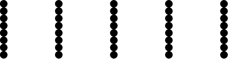
Refer to caption — Figure 1. An example to keep in mind: $\sim\delta^{-1/2}$ columns, each consisting of $\sim\delta^{-1/2}$ adjacent discs of radius $\delta$ .

For instance, the standard counterexample in Figure 1 portrays a $\delta$ -discretised $1$ -dimensional set, which projects into an essentially $1/2$ -dimensional $\delta$ -discretised set in $\sim\delta^{-1/2}$ $\delta$ -separated directions around the vertical one. Nonetheless, there are no fans to be seen, and the reason is precisely the lack of separation for the directions of small projection.

3. Proof of the main theorem

3.1. Finding a fan

As announced, the first step of the proof is to use the hypothetical (almost) sharpness of Kaufman’s bound to find a fan structure, which is defined in Claim 3.4 below. For this purpose, we can make do with weaker assumptions than those in Theorem 1.6: we consider a finite set $B\subset B(0,2)$ , consisting of $\sim\delta^{-1}$ $\delta$ -separated points and satisfying the $(\delta,1)$ -set inequality

(3.1)

|B\cap B(x,r)|\lesssim\frac{r}{\delta},\qquad x\in\mathbb{R}^{2},\>r\geq\delta.

We will later apply the conclusions to $B=A\times A$ , which clearly satisfies (3.1). Moreover, for this subsection, it suffices to assume that the angles in $E$ satisfy the $(\delta,s)$ -set criterion,

(3.2)

|E\cap B(x,r)|\lesssim\left(\frac{r}{\delta}\right)^{s},\qquad x\in S^{1},\>\delta\leq r\leq 1,

which is weaker than $\delta^{s}$ -separation. Finally, for convenience, we will assume that $E$ is a subset of $S^{1}$ instead of $\mathbb{R}$ , and that $e_{0}:=\tfrac{1}{\sqrt{2}}(1,1)\in E$ .²² 2 This assumption will eventually be used to control the size of $\pi_{e_{0}}(A\times A)=A+A$ . If $e_{0}\notin E$ , the proof runs the same way by considering $A\times xA$ , where we have good control for $A+xA$ .

Definition 3.3.

A tube $T\subset\mathbb{R}^{2}$ of width $2\delta$ is $\sigma$ -good, if for some absolute constant $c\geq 1$ ,

\mathop{\sum_{x,y\in B\cap T}}_{x\neq y}|x-y|^{s-1}\lesssim\delta^{2(s-1)+c(\sigma-s)}\log^{3/2}\left(\frac{1}{\delta}\right).

Claim 3.4.

Assume that $E$ contains $\gtrsim\delta^{-\sigma}$ directions for some $0<\sigma<s$ and satisfies (3.2). Also, assume that for each $e\in E$ , the projection $\pi_{e}(B)$ only contains $\lesssim\delta^{-s}$ $\delta$ -separated points. Then, there exists a constant $\tau=\tau(\sigma,s)>0$ and a point $b_{0}\in B$ with the following property. There is a subset $E^{\prime}\subset E$ , and for each $e\in E^{\prime}$ a $\sigma$ -good $2\delta$ -tube $T_{e}(b_{0})$ containing $b_{0}$ such that

(3.5)

\left|B\cap\bigcup_{e\in E^{\prime}}T_{e}(b_{0})\right|\gtrsim\delta^{\tau-1}.

Furthermore, $\tau(\sigma,s)\to 0$ , as $\sigma\to s$ .

Proof of claim.

The first step is to find plenty of good tubes to play with. For each $e\in E$ , partition $\mathbb{R}^{2}$ into tubes of width $2\delta$ perpendicular to $e$ . Then, fix $N\sim\delta^{-s}$ and, for each $e\in E$ , pick exactly $N$ of these tubes $T_{e,1},\ldots,T_{e,N}$ such that

B\subset\bigcup_{n=1}^{N}T_{e,n},\qquad e\in E.

This is possible by the assumption on $\pi_{e}(B)$ . The next estimation shows that, on average, the tubes $T_{e,n}$ are $\sigma$ -good:

	$\displaystyle\frac{1}{\|E\|N}\sum_{e\in E}\sum_{n=1}^{N}\mathop{\sum_{x,y\in B\cap T_{e,n}}}_{x\neq y}\|x-y\|^{s-1}$	$\displaystyle=\frac{1}{\|E\|N}\mathop{\sum_{x,y\in B}}_{x\neq y}\sum_{e\in E}\sum_{n=1}^{N}\|x-y\|^{s-1}\chi_{(x,y)\in T_{e,n}^{2}}(x,y)$
		$\displaystyle\lesssim\frac{1}{\|E\|N}\mathop{\sum_{x,y\in B}}_{x\neq y}\|x-y\|^{-1}\lesssim\frac{\delta^{-2}}{\|E\|N}\log\left(\frac{1}{\delta}\right)$
		$\displaystyle\sim\delta^{\sigma+s-2}\log\left(\frac{1}{\delta}\right)=\delta^{2(s-1)+(\sigma-s)}\log\left(\frac{1}{\delta}\right).$

Pick a large constant $C>0$ , and discard all the directions $e\in E$ such that

\frac{1}{N}\sum_{n=1}^{N}\mathop{\sum_{x,y\in B\cap T_{e,n}}}_{x\neq y}|x-y|^{s-1}\geq C\delta^{\sigma+s-2}\log\left(\frac{1}{\delta}\right).

The remaining directions are called $E_{0}$ , and the preceding computation shows that $|E_{0}|\gtrsim|E|\sim\delta^{-s}$ for large enough $C$ . Next, for all $e\in E_{0}$ , discard the tubes $T_{e,n}$ such that

\mathop{\sum_{x,y\in B\cap T_{e,n}}}_{x\neq y}|x-y|^{s-1}\geq D\delta^{\sigma+s-2}\log\left(\frac{1}{\delta}\right),

where $D\sim\sqrt{\log(1/\delta)}\delta^{(\sigma-s)/2}$ is a constant to be determined shortly. We wish to make sure that not too many points of $B$ lie in the discarded tubes. By definition of $E_{0}$ , the number of the discarded tubes, the family of which is denoted by $\mathcal{T}_{e}^{b}$ , is bounded by $|\mathcal{T}_{e}^{b}|\leq(C/D)N$ . Combining this fact, plus the definition of $E_{0}$ , and the Cauchy-Schwarz estimate

\frac{1}{N}\sum_{n=1}^{N}\mathop{\sum_{x,y\in B\cap T_{e,n}}}_{x\neq y}|x-y|^{s-1}\gtrsim\frac{1}{N}\sum_{T\in\mathcal{T}_{e}^{b}}|B\cap T_{e,n}|^{2}\gtrsim\frac{1}{(C/D)^{2}N^{2}}\left(\sum_{T\in\mathcal{T}_{e}^{b}}|B\cap T_{e,n}|\right)^{2}

shows that

\left|B\cap\bigcup_{T\in\mathcal{T}_{e}^{b}}T\right|\lesssim\sqrt{C\log(1/\delta)\delta^{\sigma+s-2}}\cdot(C/D)N\sim\frac{C^{3/2}}{D}\delta^{-1+(\sigma-s)/2}\sqrt{\log(1/\delta)}.

In other words, since $|B|\sim\delta^{-1}$ , one can choose $D\sim C^{3/2}\sqrt{\log(1/\delta)}\delta^{(\sigma-s)/2}$ so large that the following holds: for each good direction $e\in E_{0}$ , the points of $B$ covered by the "bad" tubes in $\mathcal{T}_{e}^{b}$ only constitute a $1/10$ of all the points in $B$ ; hence, if $\mathcal{T}_{e}:=\{T_{e,1},\ldots,T_{e,N}\}\setminus\mathcal{T}_{e}^{b}$ , we have

(3.6)

\left|B\cap\bigcup_{T\in\mathcal{T}_{e}}T\right|\gtrsim|B|\sim\delta^{-1},

and for all $T\in\mathcal{T}_{e}$

\mathop{\sum_{x,y\in B\cap T}}_{x\neq y}|x-y|^{s-1}\leq D\delta^{\sigma+s-2}\log\left(\frac{1}{\delta}\right)\lesssim\delta^{2(s-1)+2(\sigma-s)}\log^{3/2}\left(\frac{1}{\delta}\right),

which means that the tubes in $\mathcal{T}_{e}$ are $\sigma$ -good.

Next, we start looking for a "fan" structure. Given $b,b^{\prime}\in B$ , $b\neq b^{\prime}$ , and $e\in E_{0}$ , let $b\sim_{e}b^{\prime}$ stand for the relation of $b$ and $b^{\prime}$ sharing a tube in $\mathcal{T}_{e}$ . First, we make a quick calculation concerning the number of pairs $(b,b^{\prime})$ such that $b\sim_{e}b^{\prime}$ for some $e\in E_{0}$ . Assume that every tube in $\mathcal{T}_{e}$ contains at least two points of $B$ (if this is not the case, discard the single-point tubes, and use $|\mathcal{T}_{e}|\leq N\sim\delta^{-s}$ to conclude that (3.6) still holds for the remaining family of tubes). Then, from Cauchy-Schwarz and (3.6),

	$\displaystyle\|\{(b,b^{\prime}):b\sim_{e}b^{\prime}\}\|$	$\displaystyle\gtrsim\sum_{T\in\mathcal{T}_{e}}\|B\cap T\|^{2}$
		$\displaystyle\geq\frac{1}{\|\mathcal{T}_{e}\|}\left(\sum_{T\in\mathcal{T}_{e}}\|B\cap T\|\right)^{2}\gtrsim\delta^{s-2},$

and so, recalling that $|E_{0}|\gtrsim\delta^{-\sigma}$ ,

(3.7)

\sum_{b,b^{\prime}\in B}|\{e\in E_{0}:b\sim_{e}b^{\prime}\}|=\sum_{e\in E_{0}}|\{(b,b^{\prime}):b\sim_{e}b^{\prime}\}|\gtrsim\delta^{s-\sigma-2}.

Assume that the conclusion of our claim, namely (3.5), fails for every $b_{0}=b\in B$ , and for some

(3.8)

\tau>\frac{s-\sigma}{1-s}.

Fixing $b\in B$ , this information can be used to bound the quantity

\sum_{b^{\prime}\in B}|\{e\in E_{0}:b\sim_{e}b^{\prime}\}|

from above as follows. First, the non-concentration condition (3.2) for $E$ , thus $E_{0}$ , gives the universal bound

(3.9)

|\{e\in E_{0}:b\sim_{e}b^{\prime}\}|\lesssim\frac{1}{|b-b^{\prime}|^{s}},

simply because the set of possible directions $e\in S^{1}$ such that $b\sim_{e}b^{\prime}$ are contained in two arcs of length $\lesssim\delta/|b-b^{\prime}|$ . For $e\in E_{0}$ and $b\in B$ , let $T_{e}(b)$ be the unique tube $T_{e,n}$ containing $b$ , if $T_{e,n}\in\mathcal{T}_{e}$ , and let $T_{e}(b)=\emptyset$ otherwise. If

b^{\prime}\notin B\cap\bigcup_{e\in E_{0}}T_{e}(b)=:G(b),

then simply

\{e\in E_{0}:b\sim_{e}b^{\prime}\}=\emptyset.

Hence,

\sum_{b,b^{\prime}}|\{e\in E_{0}:b\sim_{e}b^{\prime}\}|\lesssim\sum_{b\in B}\sum_{b^{\prime}\in G(b)}\frac{1}{|b-b^{\prime}|^{s}}.

For $\delta\leq 2^{j}\leq 1$ , consider the sets $A_{j}(b):=\{b^{\prime}\in G(b):|b-b^{\prime}|\sim 2^{j}\}$ , for which the non-concentration inequality (3.1) gives the bound

|A_{j}(b)|\lesssim\min\left\{\frac{2^{j}}{\delta},\delta^{\tau-1}\right\}\leq\left(\frac{2^{j}}{\delta}\right)^{s}\cdot\delta^{(\tau-1)(1-s)}.

Plugging this into the previous equation gives

	$\displaystyle\sum_{b,b^{\prime}}\|\{e\in E_{0}:b\sim_{e}b^{\prime}\}\|$	$\displaystyle\lesssim\sum_{b\in B}\sum_{\delta\leq 2^{j}\leq 1}\sum_{b^{\prime}\in A_{j}(B)}\frac{1}{\|b-b^{\prime}\|^{s}}$
		$\displaystyle\lesssim\sum_{b\in B}\sum_{\delta\leq 2^{j}\leq 1}2^{-js}\left(\frac{2^{j}}{\delta}\right)^{s}\cdot\delta^{(\tau-1)(1-s)}$
		$\displaystyle\sim\|B\|\cdot\log\left(\frac{1}{\delta}\right)\cdot\delta^{-1+\tau(1-s)}\sim\delta^{-2+\tau(1-s)}\cdot\log\left(\frac{1}{\delta}\right).$

This upper bound contradicts a combination of (3.7) and (3.8). The claim is hence established for any $\tau(\sigma,s)>(s-\sigma)/(1-s)$ . In other words, we have found a point $b_{0}\in B$ such that $|G(b_{0})|\gtrsim\delta^{\tau-1}$ . Finally, for this particular $b_{0}$ , let $E^{\prime}\subset E_{0}$ consist of those directions such that $T_{e}(b_{0})\neq\emptyset$ (which implies that $T_{e}(b_{0})\in\mathcal{T}_{e}$ for $e\in E^{\prime}$ ). ∎

3.2. Using the fan

As stated, we apply the claim with $B=A\times A$ . In the second – and final – phase of the proof, we will need the full strength of the hypotheses. The key idea is borrowed from J. Solymosi [8]: if a product set of the form $A\times A$ is (to a large extent) contained in a "fan" of thin tubes, such as $\bigcup T_{e}(b_{0})$ , then the sumset $A+A$ has quantitatively larger size than $A$ .

To prove this, we assume, without loss of generality, that $E^{\prime}=E$ , that the directions in $E$ lie in the northeast quartile $Q$ of $\mathbb{R}^{2}$ , and also that

(3.10)

\left|(A\times A)\cap\bigcup_{e\in E}T_{e}(b_{0})\cap(b_{0}+Q)\right|\gtrsim\delta^{\tau-1}.

In English, a significant part of the points in $(A\times A)\cap\bigcup T_{e}(b_{0})$ is contained to the northeast of $b_{0}$ . The rest of the points in $A\times A$ are not needed, so we assume that $(A\times A)\cap T_{e}(b_{0})$ is contained in the quartile $b_{0}+Q$ for every $e\in E$ .

Write

\kappa:=\kappa(\sigma,s):=\max\{\tau(\sigma,s),c(s-\sigma)\}.

For each tube $e\in E^{\prime}$ , discard all the points $x\in(A\times A)\cap T_{e}(b_{0})$ such that

(3.11)

\mathop{\sum_{y\in(A\times A)\cap T_{e}(b_{0})}}_{x\neq y}|x-y|^{s-1}\geq C\delta^{s-1-2\kappa}\log^{3/2}\left(\frac{1}{\delta}\right)

for a large constant $C>0$ . Since $T_{e}(b_{0})$ is a good tube, the number of such points is bounded by $\lesssim\delta^{s-1+\tau}/C$ , and since the number of tubes $T_{e}(b_{0})$ , $e\in E$ , is bounded by $\lesssim\delta^{-s}$ , we find that only $\lesssim\delta^{\tau-1}/C$ points $x\in A\times A$ were discarded altogether. Hence, choosing $C>0$ large enough, (3.10) continues to hold with $A\times A$ replaced by the set of remaining points, and moreover we can now assume that the inequality opposite to (3.11) holds for all $x\in A\times A$ and $e\in E$ . We will use this fact in the slightly weaker form

(3.12)

|(A\times A)\cap T_{e}(b_{0})\cap B(x,r)|\lesssim\delta^{-2\kappa}\log^{3/2}\left(\frac{1}{\delta}\right)\cdot\left(\frac{r}{\delta}\right)^{1-s},\quad x\in\mathbb{R}^{2},\;r\geq\delta.

We also need to arrange so that there are no points of $A\times A$ too close to $b_{0}$ : we throw away all the points $x\in A\times A$ that lie in a ball $B(b_{0},C\delta^{1-s})$ , where $C>0$ is an absolute constant large enough for future purposes. This removal procedure only costs $\lesssim C\delta^{1-s}/\delta=C\delta^{-s}$ points according to the non-concentration inequality for $A$ , so (3.10) remains valid for small enough $\delta>0$ .

Observe that (3.12) combined with the assumption $A\times A\subset B(0,1)$ implies that any tube $T_{e}(b_{0})$ , $e\in E$ , can contain at most $\lesssim\delta^{-2\kappa}\log^{3/2}(1/\delta)\cdot\delta^{s-1}$ points of $A\times A$ . Combined with (3.10) and $|E|\lesssim\delta^{-s}$ , this means that there exists a subcollection $\mathcal{T}$ of the tubes $T_{e}(b_{0})$ of cardinality

(3.13)

|\mathcal{T}|\gtrsim\delta^{3\kappa}\log^{-3/2}\left(\frac{1}{\delta}\right)\cdot\delta^{-s}\gtrsim\delta^{4\kappa-s}

such that

(3.14)

|(A\times A)\cap T|\gtrsim\delta^{\kappa+s-1},\qquad T\in\mathcal{T}.

In the sequel, only these tubes will be of interest, and we enumerate them, $\mathcal{T}=\{T_{1},\ldots,T_{N}\}$ , so that tubes with consecutive indices correspond to consecutive directions in $E$ .

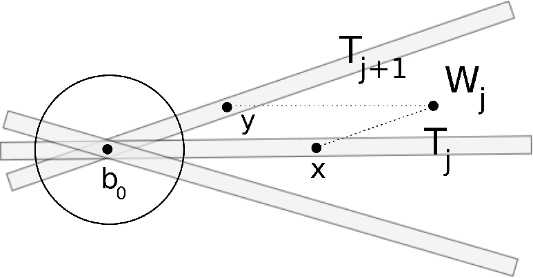
The next, and final, step of the proof is to consider vector sums of the form

(3.15)

b_{0}+(x-b_{0})+(y-b_{0})=(x+y)-b_{0},

where $x\in(A\times A)\cap T_{j}$ and $y\in(A\times A)\cap T_{j+1}$ for some $1\leq j\leq N-1$ , see Figure 2. Such vector sums are always contained in the conical region spanned by two boundary lines of the tubes $T_{j}$ and $T_{j+1}$ . A fortiori, if $x,y$ lie outside the ball $B(b_{0},C\delta^{1-s})$ for large enough $C$ , then elementary geometry and the $\delta^{s}$ -separation of the directions $e\in E$ gives that the sum in (3.15) will be contained in the white conical region $W_{j}$ outside the tubes $T_{e}(b_{0})$ , depicted in Figure 2. The regions $W_{j}$ are disjoint for distinct pairs of consecutive tubes, so the plan is to find many $\delta$ -separated vector sums in each $W_{j}$ , and then multiply by their number $|W_{j}|=N-1$ . By definition, the vector sums of the form (3.15) are contained in the set

(A\times A)+(A\times A)-b_{0}=(A+A)\times(A+A)-b_{0},

so finding many $\delta$ -separated vector sums will result in a lower bound for the number of $\delta$ -separated points in $(A+A)\times(A+A)$ , and hence $A+A$ .

Now, we start forming the vector sums from pairs of points in $(A\times A)\cap T_{j}$ and $(A\times A)\cap T_{j+1}$ . We wish to find $\delta$ -separated such sums, so we need to compute, how many vector sums can land within a distance $\delta$ of each other. Here the separation of the directions in $E$ is essential.

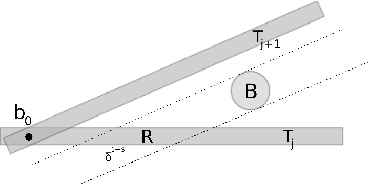
Given an arbitrary $\delta$ -ball $B\subset W_{j}$ , it is only possible for the sum $(x+y)-b_{0}$ to hit $B$ , if $x\in T_{j}$ , say, is chosen inside a rectangle $R\subset T_{j}$ of dimensions $\sim\delta^{1-s}\times\delta$ . For any such $x$ , there are only $\lesssim 1$ choices of $y\in(A\times A)\cap T_{j}$ such that $(x+y)-b_{0}\in B$ . Applying the non-concentration inequality (3.12), we may conclude that there exist at most

\lesssim\delta^{-2\kappa}\log^{3/2}\left(\frac{1}{\delta}\right)\cdot\left(\frac{\delta^{1-s}}{\delta}\right)^{1-s}\lesssim\delta^{s(s-1)-3\kappa}

pairs $(x,y)$ such that $x\in(A\times A)\cap T_{j}$ , $y\in(A\times A)\cap T_{j+1}$ , and $(x+y)-b_{0}\in B$ .

The conclusion above holds for an arbitrary $\delta$ -ball $B\subset W_{j}$ , so the we may estimate the number of $\delta$ -separated sums $(x+y)-b_{0}\in W_{j}$ from below by

\gtrsim\delta^{s(1-s)+3\kappa}\cdot|(A\times A)\cap T_{j}|\cdot|(A\times A)\cap T_{j+1}|\gtrsim\delta^{s(1-s)+5\kappa+2(s-1)}=\delta^{5\kappa+(2-s)(s-1)},

the second inequality being the content of (3.14). Summing up the contributions from the various regions $W_{j}$ , $1\leq j\leq N-1$ , and recalling that $N\gtrsim\delta^{4\kappa-s}$ by (3.13), we obtain altogether

\gtrsim\delta^{9\kappa+(2-s)(s-1)-s}=\delta^{9\kappa+2s-s^{2}-2}

$\delta$ -separated sums of the form $(x+y)-b_{0}$ . As we observed earlier, this means that the set $(A+A)\times(A+A)-b_{0}$ contains at least this many $\delta$ -separated points, and so $A+A$ contains at least

\gtrsim\delta^{5\kappa+s-s^{2}/2-1}

$\delta$ -separated points. Finally recall that our starting assumption was that $A+A$ only contains $\lesssim\delta^{-s}$ $\delta$ -separated points. This forces

\delta^{5\kappa+s-s^{2}/2-1}\lesssim\delta^{-s},

which in the range $s<2-\sqrt{2}$ this gives a lower bound for $\kappa$ – and hence an upper bound for $\sigma<s$ , because $\kappa\to 0$ , as $\sigma\to s$ . The proof of Theorem 1.6 is complete.

Appendix A Finding many points on a line

This final section contains the proof of Theorem 2.3, repeated below:

Theorem A.1.

Let $P\subset\mathbb{R}^{2}$ be a finite set with $|P|=n$ . Let $s\geq 1/2$ , and assume that $G\subset P\times P$ is a set of pairs of cardinality $|G|\geq n^{1+s}$ such that

|S(G)|\leq\frac{cn^{2s-1}}{\log^{12}n}

We establish the sharpness claims first through two examples; this will hopefully illustrate, where the numerology in the exponents comes from. The first example, a simple grid with $n$ points, shows that the assumption $|S(G)|\lesssim n^{2s-1}$ is insufficient for the desired conclusion:

Example A.2.

Let $P=\{0,\ldots,n^{1/2}\}\times\{0,\ldots,n^{1/2}\}$ . Write $r:=n^{s-1/2}$ , and let $P_{r}:=\{p\in P:|p|\leq r\}$ . Then $|P_{r}|\sim r^{2}$ , and the various pairs of points in $P_{r}$ span $\sim r^{2}$ slopes. As one easily checks, for each of these slopes $e$ , there are $\gtrsim n^{3/2}/r$ pairs $(p,q)\in P\times P$ such that $s(p,q)=e$ . So, we can find $\gtrsim r^{2}\cdot n^{3/2}/r=r\cdot n^{3/2}=n^{1+s}$ pairs spanning $\sim r^{2}=n^{2s-1}$ slopes. In particular, the assumptions $|G|\gtrsim n^{1+s}$ and $S(G)\lesssim n^{2s-1}$ do not guarantee a line $\ell$ with $|\ell\cap P|\gg n^{1/2}$ .

The second example shows, that the strengthening the assumption to $|S(G)|\leq n^{t}$ , $t<2s-1$ , is useless in view of the conclusion:

Example A.3.

Fix $1/2<s<1$ , draw $k\sim n^{1-s}$ parallel lines, with slope $e$ , say, and place $n/k\sim n^{s}$ points on each line. Call these points $P$ . Then $|P|=n$ , and there are $(n/k)^{2}\cdot k=n^{2}/k\sim n^{1+s}$ pairs in $(p,q)\in P\times P$ with $s(p,q)=e$ . If $G$ is the set of those pairs, we have $|G|\gtrsim n^{1+s}$ and $S(G)=1\lesssim n^{t}$ for any $t>0$ .

Finally, we prove Theorem 2.3:

Proof of Theorem 2.3.

By assumption, slopes of the pairs in $G$ are contained in a set $E\subset S^{1}$ of cardinality $|E|\ll n^{2s-1}/\log^{12}n$ . For $j\geq 0$ , let $E_{j}\subset E$ be the subset of slopes $e$ , for which there exist between $2^{j}$ and $2^{j+1}$ pairs $(p,q)\in G$ with $s(p,q)=e$ . Then

n^{1+s}\leq|G|\sim\sum_{j=0}^{\infty}|E_{j}|\cdot 2^{j},

so there exists $j\geq 0$ with

(A.4)

\frac{n^{1+s}}{2^{j}\cdot j^{2}}\lesssim|E_{j}|\lesssim\frac{n^{1+s}}{2^{j}}.

Moreover, $j$ can be chosen rather large. Namely, for $T\in\mathbb{N}$ ,

\sum_{j=0}^{T}|E_{j}|\cdot 2^{j}\leq\sum_{j=0}^{T}|E|\cdot 2^{j}\leq\frac{cn^{2s-1}}{\log^{12}n}\sum_{n=0}^{T}2^{j}\sim\frac{cn^{2s-1}}{\log^{12}n}\cdot 2^{T},

and this is $\ll|G|=n^{1+s}$ , as long as $2^{T}\ll c^{-1}n^{2-s}\cdot\log^{12}n$ . Consequently, $j$ can be chosen satisfying (A.4) and

(A.5)

2^{j}\geq Cn^{2-s}\cdot\log^{12}n,

where $C$ can be made large by assuming that $c$ is small.

Fix $j$ with these good properties. Then, for each $e\in E_{j}$ , let $\mathcal{L}_{e,k}$ , $k\geq 0$ , be the set of lines with slope $e$ , which contain between $2^{k}$ and $2^{k+1}$ points of $P$ . Since there are $\sim 2^{j}$ pairs of $G\subset P\times P$ contained on such lines, one has

2^{j}\lesssim\sum_{k=0}^{\infty}|\mathcal{L}_{e,k}|\cdot 2^{2k}.

Consequently, there exists $k\geq 0$ satisfying

(A.6)

|\mathcal{L}_{e,k}|\gtrsim\frac{2^{j}}{2^{2k}\cdot k^{2}}.

As before, $k$ can be chosen fairly large. Namely, the cardinality of $\mathcal{L}_{e,k}$ is always bounded by $|\mathcal{L}_{e,k}|\lesssim n/2^{k}$ , so for $T\in\mathbb{N}$ one has the estimate

\sum_{j=0}^{T}|\mathcal{L}_{e,k}|\cdot 2^{2k}\lesssim n\cdot\sum_{j=0}^{T}2^{k}\lesssim n\cdot 2^{T}.

The left hand side is $\ll 2^{j}$ , as long as $2^{T}\ll 2^{j}/n$ , and this means that $k\geq 0$ can be found satisfying (A.6) and

(A.7)

2^{k}\gtrsim\frac{2^{j}}{n}\geq Cn^{1-s}\cdot\log^{12}n,

where the latter inequality follows from (A.5). Now, this $k$ depends on $e$ , of course, but by pigeonholing once more – and observing that $2^{k}\lesssim n$ – one can find a subset $E^{\prime}_{j}\subset E_{j}$ of cardinality

\frac{|E_{j}|}{\log n}\lesssim|E_{j}^{\prime}|\leq|E_{j}|

such that the same $k$ works for all $e\in E_{j}^{\prime}$ . Finally, for all $e\in E_{j}^{\prime}$ , remove some lines from $\mathcal{L}_{e,k}$ until $\lesssim 2^{j-2k}$ lines remain; this is possible by (A.6).

The proof is completed by appealing to the Szemerédi-Trotter theorem [9], which asserts that the incidences $I(\mathcal{L},P)=\{(\ell,p):\ell\in\mathcal{L},\>p\in\ell\cap P\}$ between a family of lines $\mathcal{L}$ and a family of points $P$ satisfies

|I(\mathcal{L},P)|\lesssim|\mathcal{L}|^{2/3}|P|^{2/3}+|\mathcal{L}|+|P|.

Here, let $\mathcal{L}$ be the family of all the lines in all the (possibly reduced) collections $\mathcal{L}_{e,k}$ , for $e\in E_{j}^{\prime}$ . By (A.4) and (A.6), the cardinality of $\mathcal{L}$ is bounded from below and above as follows:

\frac{n^{1+s}}{2^{2k}\cdot\log^{4}n}\lesssim\frac{n^{1+s}}{2^{2k}\cdot(jk)^{2}}\lesssim|\mathcal{L}|\lesssim\frac{n^{1+s}}{2^{2k}}.

Each line in $\mathcal{L}$ contains $\sim 2^{k}$ points of $P$ , so the number of incidences $I(\mathcal{L},P)$ between $\mathcal{L}$ and $P$ is $\gtrsim n^{1+s}/(2^{k}\cdot\log^{4}n)$ . Plugging this into the Szemerédi-Trotter bound yields

\frac{n^{1+s}}{2^{k}\cdot\log^{4}n}\lesssim\left(\frac{n^{1+s}}{2^{2k}}\right)^{2/3}\cdot n^{2/3}+\frac{n^{1+s}}{2^{2k}}+n=\frac{n^{4/3+2s/3}}{2^{4k/3}}+\frac{n^{1+s}}{2^{2k}}+n.

There are three possible cases, according to which one of the three terms on the right dominates. The first term cannot do this, because the resulting inequality combined with (A.7) – for large enough $C$ – would lead to a contradiction:

Cn^{1-s}\cdot\log^{12}n\lesssim 2^{k}\lesssim n^{1-s}\cdot\log^{12}n.

The same is true of the second term, for the same reason. So, the third term dominates, and this gives

2^{k}\gtrsim\frac{n^{s}}{\log^{4}n}.

The proof is complete, because the lines on $\mathcal{L}$ contain $\gtrsim 2^{k}$ points. ∎

References

[1] J. Bourgain: The discretised sum-product and projection theorems, J. Anal. Math 112 (2010), pp. 193–236
[2] K. Fässler and T. Orponen: On restricted families of projections in $\mathbb{R}^{3}$ , to appear in Proc. London Math. Soc., also available at arXiv:1302.6550
[3] R. Kaufman: On Hausdorff dimension of projections, Mathematika 15 (1968), pp. 153–155
[4] R. Kaufman and P. Mattila: Hausdorff dimension and exceptional sets of linear transformations, Ann. Acad. Sci. Fenn. Math. 1 (1975), pp. 387–392
[5] N. Katz and T. Tao: Some connections between Falconer’s distance set conjecture, and sets of Furstenberg type, New York J. Math. 7 (2001), pp. 149–187
[6] D. Oberlin: Restricted Radon transforms and projections of planar sets, published electronically in Canadian Math. Bull. (2014), also available at arXiv:0805.1678
[7] T. Orponen: On the packing dimension and category of exceptional sets of orthogonal projections, to appear in Ann. Mat. Pura Appl., also available at arXiv:1204.2121
[8] J. Solymosi Bounding multiplicative energy by the sumset, Adv. Math. 222, Issue 2 (2009), pp. 402–408
[9] E. Szemerédi and W. T. Trotter: Extremal problems in discrete geometry, Combinatorica 3(3) (1983), pp. 381–392
[10] P. Ungar: $2N$ noncollinear points determine at least $2N$ directions, J. Combinatorial Theory, Ser. A 33 (1982), pp. 343–347

	$\displaystyle\frac{1}{\|E\|N}\sum_{e\in E}\sum_{n=1}^{N}\mathop{\sum_{x,y\in B\cap T_{e,n}}}_{x\neq y}\|x-y\|^{s-1}$	$\displaystyle=\frac{1}{\|E\|N}\mathop{\sum_{x,y\in B}}_{x\neq y}\sum_{e\in E}\sum_{n=1}^{N}\|x-y\|^{s-1}\chi_{(x,y)\in T_{e,n}^{2}}(x,y)$
		$\displaystyle\lesssim\frac{1}{\|E\|N}\mathop{\sum_{x,y\in B}}_{x\neq y}\|x-y\|^{-1}\lesssim\frac{\delta^{-2}}{\|E\|N}\log\left(\frac{1}{\delta}\right)$
		$\displaystyle\sim\delta^{\sigma+s-2}\log\left(\frac{1}{\delta}\right)=\delta^{2(s-1)+(\sigma-s)}\log\left(\frac{1}{\delta}\right).$

	$\displaystyle\sum_{b,b^{\prime}}\|\{e\in E_{0}:b\sim_{e}b^{\prime}\}\|$	$\displaystyle\lesssim\sum_{b\in B}\sum_{\delta\leq 2^{j}\leq 1}\sum_{b^{\prime}\in A_{j}(B)}\frac{1}{\|b-b^{\prime}\|^{s}}$
		$\displaystyle\lesssim\sum_{b\in B}\sum_{\delta\leq 2^{j}\leq 1}2^{-js}\left(\frac{2^{j}}{\delta}\right)^{s}\cdot\delta^{(\tau-1)(1-s)}$
		$\displaystyle\sim\|B\|\cdot\log\left(\frac{1}{\delta}\right)\cdot\delta^{-1+\tau(1-s)}\sim\delta^{-2+\tau(1-s)}\cdot\log\left(\frac{1}{\delta}\right).$