Evolution of geodesic congruences in a gravitationally collapsing scalar field background
Abstract
The evolution of timelike geodesic congruences in a spherically symmetric, nonstatic, inhomogeneous spacetime representing gravitational collapse of a massless scalar field is studied. We delineate how initial values of the expansion, rotation and shear of a congruence, as well as the spacetime curvature, influence the global behavior and focusing properties of a family of trajectories. Under specific conditions, the expansion scalar is shown to exhibit a finite jump (from negative to positive value) before focusing eventually occurs. This nonmonotonic behavior of the expansion, observed in our numerical work, is successfully explained through an analysis of the equation for the expansion. Finally, we bring out the role of the metric parameters (related to nonstaticity and spatial inhomogeneity), in shaping the overall behavior of geodesic congruences.
I Introduction
In general relativity (GR), the behavior of a family of test particles (described by a nonspacelike geodesic congruence), in a given spacetime background, is analyzed by studying the evolution of three kinematic variables– expansion, shear, and rotation (ESR). The evolution of the ESR along the congruence, is governed by the Raychaudhuri equations [1, 2, 3]. It is well known that the Raychaudhuri equations play a crucial role in the context of the Penrose-Hawking singularity theorems [4, 5].
The structure and geometric features of a given spacetime (encoded in the metric and its derivatives) must necessarily be reflected in the evolution of the kinematic variables that characterize a geodesic congruence. Apart from initial conditions on the kinematic variables, geometric quantities (e.g., the Ricci tensor, Ricci scalar, and the Weyl tensor) that appear in the Raychaudhuri equations, also influence the evolution of the congruence. Thus, knowing the kinematics of geodesic congruences surely helps in probing the spacetime geometry. In addition, we know that, observationally, one of the ways to verify the existence and nature of a given spacetime geometry (and the gravitational field it represents) is through a study of trajectories.
The evolution of the kinematic variables of timelike geodesic congruences has been extensively studied in various spacetime backgrounds in the recent past [6, 7, 8]. However, much of this earlier work has been in spacetimes that are static. Studies on the evolution of geodesic congruences in spherically symmetric, inhomogeneous, nonstatic spacetimes such as those representing gravitational collapse have not been looked at yet. One might expect that issues specific to collapsing scenarios, which include the formation of singularities, apparent horizons, conjectures, theorems related to singularities etc., may be understood through such studies.
An important and well-known result that follows from the Raychaudhuri equation for the expansion is that of geodesic focusing. A congruence has a focal point if all geodesics in the family converge and meet there, at a finite value of the affine parameter. Geodesic focusing may be completely benign; i.e., a focal point may not be a curvature singularity, but the geodesics in a family intersect at such a focal point, thereby defining the notion of a congruence singularity. On the other hand, curvature singularities must always be focal points of a geodesic congruence.
Even though much has been said and proved about geodesic focusing, questions do remain. In particular, the questions we wish to analyze are largely related to detailed studies from which, some surprises may emerge. Some such questions are as follows:
How and in what ways do the initial values of ESR influence the occurrence of focusing/defocusing?
What are the precise roles of spacetime curvature and other geometric quantities in the evolution of congruences?
Besides monotonic focusing and defocusing, are there any other characteristic features in the evolution of the expansion, shear, or rotation that may be correlated with properties of a given spacetime geometry?
By adopting methods developed in some of our earlier papers [6, 7, 8], in this article, we try to answer some of these questions in the context of a class of spherically symmetric, nonstatic, inhomogeneous spacetimes representing gravitational collapse.
Of course, in order to proceed with our studies, we need a spacetime line element representing gravitational collapse. Among many available models, we choose an exact solution representing a scalar field collapse scenario in (3+1) dimensions [9]. Our choice is essentially governed by an available exact, spherically symmetric, nonstatic, inhomogeneous solution that is reasonably simple in its line element structure. However, note that in this solution the scalar field is all pervading (exists for all and ) and the collapse scenario is somewhat different from the usual pressureless dust ball collapse (Oppenheimer-Snyder) or even the spherisymmetric collapse of a perfect fluid with pressure.
The above-mentioned spacetime, along with its geodesic structure is discussed in Sec. II. In Sec. III, we briefly review the derivation of the Raychaudhuri equations for geodesic congruences. In Sec. IV, we solve the ESR evolution equations (along with the geodesic equations) numerically and bring out certain aspects of the evolution kinematics of the congruence. An interesting behavior of the expansion under specific conditions is explained in a general context in Sec. V. The role of the metric parameters related to nonstaticity and spatial inhomogeneity in controlling and characterizing the evolution of congruences is studied in Sec. VI. Finally, Sec. VII summarizes our results and suggests future avenues of work.
II Exact solution for scalar field collapse
We begin by writing the line element representing the gravitational collapse of a massless scalar field minimally coupled to (3+1)-dimensional gravity [9]
| (1) |
where
and the scalar field profile is given as,
where , , , are constants and . is the area radius.
The above line element and the scalar field constitute solutions of the Einstein field equations given as
| (2) |
The plots for the scalar field profile are shown in Fig. 1. The curvature scalar for the metric is
It should be noted that curvature singularities are present at and at for both values of . Depending on the constants , and , the metric (1) represents different types of spacetimes. Details about these solutions are available in [9]. The constant is related to the central inhomogeneity of the matter distribution. In the limit , the dependence of the metric is removed and the spacetime becomes homogeneous [10, 11]. is the nonstaticity parameter. and represent black-hole-like and white-hole-like solutions, respectively. We consider the case . The apparent horizon is described by . The time of formation of the apparent horizon at a Lagrangian coordinate is given by
| (3) |
where plus (minus) sign is for (). For , the two-sphere labeled by gets trapped () for .
The geodesics in the equatorial section of the collapsing spacetime are governed by
| (4) |
| (5) |
| (6) |
where is an integration constant representing angular momentum. In obtaining Eqs. (4)-(6), we have used the transformation . Also, we have used the fact that the velocity vector satisfies the constraint , where for timelike geodesics and for null geodesics.


III The Raychaudhuri equations
Consider a congruence of timelike geodesics in a given spacetime background. The geodesic congruence may undergo isotropic expansion, shear, and rotation (ESR). The kinematics of these quantities are investigated in the spacelike hypersurface orthogonal to the central geodesic. Therefore, one can define a transverse spatial metric induced on the spacelike hypersurface as
| (7) |
where the timelike vector field associated with the congruence is tangent to the geodesic at each point and satisfies the timelike constraint . The transverse metric satisfies , implying that is orthogonal to . From the vector field , one can define the velocity gradient tensor . In four spacetime dimensions, the tensor can be decomposed into its trace, symmetric traceless, and antisymmetric parts as
| (8) |
where is the expansion scalar (trace part), the shear tensor (symmetric traceless part) and the rotation tensor (antisymmetric part). By virtue of this construction, the shear and the rotation tensors satisfy and . We also have and . Since and , both and are purely spatial (i.e., and ) and lie in the orthogonal hypersurface.
The evolution equation for the spatial tensor can be written as,
| (9) |
where is the Riemann tensor. The trace, symmetric traceless, and antisymmetric parts of the equation yield [3]
| (10) |
| (11) |
| (12) |
where , , is the affine parameter, is the Weyl tensor and is the transverse trace-free part of . The equation for is a Riccati-type equation, and is of considerable interest in the context of the singularity theorems. Redefining , one can obtain the following Hill-type equation:
| (13) |
The analysis of focusing () or defocusing () can be done by investigating the quantity . It is clear from (10) that the sufficient condition for geodesic focusing is . Timelike convergence condition requires . Thus, from the signs of the various terms in the equation for the expansion, we can conclude that rotation defies focusing, whereas shear assists it.
In the context of this paper and from the Einstein-scalar equations, we have . Therefore,
| (14) |
The third term on the right-hand side above is always positive. Hence, the positivity of is crucially dependent on the sign of . As we see, may be positive or negative over a certain domain of . Thus, it is possible that there exists a domain of where . We see in detail later how the fact that over a restricted domain of gives rise to a distinct new feature in the evolution of the expansion scalar . In particular, we observe that the expansion scalar can exhibit a glitch or a jump in its evolution before eventually focusing.
IV Evolution of a timelike geodesic congruence
IV.1 Method of solution
Equations (10)-(12) are nonlinear coupled, ordinary differential equations. In the absence of analytical solutions, one has to solve this set of equations (along with the geodesic equations) numerically. However, instead of solving Eqs. (10)-(12), it is more convenient to solve Eq. (9) and subsequently extract the expansion scalar , shear tensor , and rotation tensor by taking the trace, symmetric traceless, and antisymmetric parts of , respectively. The initial condition on can be easily constructed from the initial conditions on the ESR variables using (8). It may be pointed out that initial conditions on the velocity field , and must satisfy the orthogonality conditions.
We first study the kinematic evolution of geodesic congruences for the black-hole-like solution (, , and ). There is a timelike singularity at , i.e., at , and a spacelike singularity at . For the latter case, the range of the time coordinate is . At time , the whole spacetime collapses to the origin . Therefore, for geodesics beginning at time , the spacelike singularity at is a future directed singularity. We consider the geodesic congruence in the equatorial section (). Throughout the numerical evaluation, we have kept fixed the initial conditions on .
IV.2 Evolution of kinematic variables for


From the numerical evaluations, with different initial conditions, it is found that the congruence always exhibits focusing. We denote as the value of the affine parameter at which focusing takes place. The dependence of on the initial conditions of the ESR variables is presented in Fig. 2. The value corresponds to the time when the geodesic congruence encounters a future spacelike singularity. Figure 3 shows the variations of and the area radius along the geodesic congruence with identically vanishing shear and rotation. It is clear that, as , the area radius tends to zero. Therefore, as , the congruence falls into the spacelike singularity. As observed in Fig. 3, the congruence encounters the apparent horizon at , after which it gets trapped () in the trapping region formed in the spacetime. The area radius initially increases untill the congruence hits the apparent horizon and is subsequently subsumed in the trapped region before it falls into the singularity. Therefore, the congruence gets trapped before it falls into the singularity. This is because of the fact that, in the given collapsing spacetime, a two-sphere labelled by becomes trapped before it becomes singular, i.e, before it collapses to the origin . The plateau-top region in Fig. 2 corresponds to the time (in terms of the affine parameter ) of formation of the spacetime singularity. We now discuss the effect of initial ESR, as well as the curvature, on the focusing time.


IV.2.1 Effect of initial expansion and shear on focusing
Generally, the effect of increasing (decreasing) the initial expansion () is to delay (prepone) the focusing, but for in a certain range, Fig. 2(a) shows a peculiar nonmonotonic dependence of on . For lying between two values and (), with decreasing , decreases up to a certain initial expansion ; below , increases suddenly and then starts decreasing again. Notice that the value of depends on .
To understand the above-mentioned peculiar behavior for , we consider the initial conditions corresponding to the section in Fig. 2(a) and plot the evolution of the expansion in Fig. 4. It is observed that untill , decreases with decreasing . However, between and , a transition (sudden change) in focusing time is noted; focusing is delayed. Therefore, for , lies between and . In Fig. 5, we investigate this peculiar behavior in the focusing time by plotting the corresponding evolution of the scalars , , , and . It is observed that, for , diverges mainly because of the curvature term , and the divergence takes place as , implying that the focusing takes place due to the singularity formation [Fig. 5(a)]. For or , diverges because of the term , and divergence takes place much before the singularity formation, implying that the focusing takes place due to divergence of shear [Figs. 5(b) and 5(c)]. For , initially and almost cancel each other in the expression of [Fig. 5(d)]. However, midway during the evolution, over a short period, dominates over making (congruence starts defocusing). This induces a sharp transition/jump (from negative to positive) in the evolution of , as shown in Fig. 4. As the evolution proceeds further, again becomes positive and diverges because of the curvature term . Therefore, the focusing is delayed (see Fig. 4) because of the dominance of rotation over shear, midway during the evolution. However, complete defocusing does not take place because diverges as the evolution proceeds toward the singularity formation time . The amplitude of the jump in the evolution of the expansion scalar gets smaller as one makes the initial expansion more negative (Fig. 4). It may again be noted that, for the case , focusing takes place entirely due to the divergence of shear [Fig. 5(f)], and the curvature singularity has no role in the focusing.
The sections of Fig. 2(b) indicate that, with increasing , focusing time decreases monotonically; i.e., initial shear always helps in focusing.
IV.2.2 Effect of initial rotation on focusing
It is well known that rotation always defies focusing. The sections of Fig. 2(c) show the dependence of on initial rotation . It is clear that increases with up to a certain critical value . At , there is a sudden change in focusing time. To understand this transition, i.e., sudden change in focusing time, we plot for and and note the change in focusing time for different initial rotation (Fig. 6). The corresponding plots for the ESR variables, and are shown in Fig. 7. Clearly, one can note a sudden change in focusing time between and . The transition takes place because of the dominance of , midway during the evolution (Figs. 7(c) and 7(d)).


IV.3 Evolution of kinematic variables for
As in the previous case, here too focusing always takes place. In Fig. 8, we show the dependence of the focusing affine parameter on the initial values of the ESR variables. In this case, the singularity formation time corresponds to .


IV.3.1 Effect of initial expansion and shear on focusing
The sections of Figs. 8(a) and 8(b) and sections of Fig. 8(c) indicate that, up to a certain initial expansion, focusing time increases with increasing . Above this certain value, focusing time is independent of because focusing always takes place at the singularity. The dependence of focusing time on the initial shear is the same as that in the case with .
IV.3.2 Effect of initial rotation on focusing
The sections of Fig. 8(a) indicate that, with zero initial shear, the focusing time is independent of rotation but with a sufficient nonzero initial shear, focusing time depends on the initial rotation [see sections of Fig. 8(d) and Fig. 9(b)]. This is due to the fact that, in the absence of any spacetime singularity formation, the congruence would have focused beyond the singularity formation time . A sufficient initial shear focuses the congruence before it falls to the singularity. This focusing now can be delayed by choosing some initial rotation. Thus, sufficient initial shear and rotation affect the focusing behavior of the congruence [Figs. 8(d) and 9(b)].
Figures 10 demonstrates the reason that is independent of initial rotation for . From the figures, it is clear that, unlike the case for , the rotation drops to small values and hence does not have a significant effect on as the evolution proceeds. Therefore, the evolution of is completely controlled either by the curvature term [Figs. 10(a) and 10(b)] or by the shear [Figs. 10(c) and 10(d)]. The transition in in Fig. 9(b) can be explained in the same way as that for the case .


From the above analysis, we observe that focusing always takes place. To illustrate this further, we draw three schematic diagrams in Fig. 11. The solid circle, red dot, and blue dot represent the position of the apparent horizon, the singularity at , and the initial position of the congruence, respectively. The region outside (inside) the apparent horizon is trapped (untrapped). The apparent horizon shrinks in size with time. As the evolution proceeds, depending on the initial conditions on the ESR variables, the congruence may get focused before hitting the apparent horizon or may hit the apparent horizon at some [Fig. 11] and get trapped. This trapped congruence gets focused either before falling into the singularity or at the singularity (third diagram). Therefore, we must always have focusing, though this may be benign (not happening at a curvature singularity) for certain initial conditions, as discussed above.
V Analysis of jump in the expansion scalar
In the last section, we noticed that midway during the evolution of the congruence, the dominance of rotation over shear (which makes ) leads to a sharp transition (from negative to positive value) in the evolution of expansion of the congruence. As the evolution proceeds further, because of the curvature term, diverges to positive infinity, thereby causing eventual focusing of the congruence. Let us first ask and analyze this question: what would happen if the curvature term does not diverge as the evolution proceeds? For example, for static spacetimes, as the family of outgoing timelike geodesics evolves, the curvature term becomes less and less significant. This is also true for this nonstatic case, except at the end of the evolution process. Therefore the value and sign of is largely determined by the values of the shear and the rotation terms. Ignoring the curvature term, we may have the following subcases:
(1) During the evolution, if there is a phase where (rotation dominates over shear) and then the shear dominates over the rotation, ultimately making , we may observe a finite jump after which the congruence will focus.
(2) If always and goes to zero as , goes to zero after a sharp transition from negative to positive value. This effect has been observed earlier in the kinematic study of a family of projectile trajectories [12] and also in the kinematic study of deformable media without stiffness [13].
(3) If oscillates between positive and negative values, we have periodic oscillations in the expansion scalar; focusing does not take place. This effect has been observed in the kinematic study of a family of trajectories in the two dimensional isotropic harmonic oscillator, a charged particle in an electromagnetic field [12] and also in the kinematic study of deformable media with stiffness [13]. In [12], and the analog of the curvature term is a constant, given by ; the total curvature oscillates between positive and negative values.
(4) If always and diverges to negative infinity at some , we may have complete defocusing of the congruence.
One of the above cases could have occurred for our spherically symmetric, nonstatic spacetime, had the singularity not formed but as the evolution proceeds toward the singularity formation time, the curvature term, and hence , diverges to positive infinity. Therefore, we have focusing following a sharp jump in the expansion scalar. If the rotation had not dominated over shear, midway during the evolution, we would have observed direct focusing without any intermediate jump in the expansion scalar.
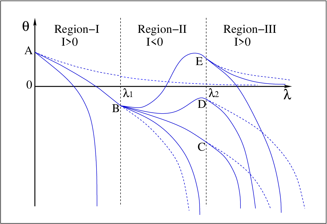
We now explain this nonmonotonic glitch/jump in the expansion before complete focusing in a general way. To do this, let us go back to the Raychaudhuri equation for the expansion given as
| (15) |
Let us assume that is negative between and and positive elsewhere (as shown in Fig. 12). What can we say about the possible behavior of in such a case? When (region I in Fig. 12), we have
| (16) |
Integrating the above inequality gives
| (17) |
where is the value of at . Hence, any expansion curve (with ) in this region I must obey the above inequality. The slope of at any must also be less than the slope of the equality curve for the expansion. The equality curve, i.e., the expansion curve for , is shown by dotted blue curve. It is possible that the expansion curve for diverges to negative infinity within this region I, thereby resulting in focusing. If it does not focus, it will hit the line at some value of (at point B, say). Taking this value as the initial , one now proceeds into region II where . In this region the inequality reads to
| (18) |
where is the value of the expansion at for some typical expansion curve in region I ending at . It is now possible for the expansion curve to turn around and enter the region II allowed by the inequality 18 in region II. In this region, if is not negative enough so that we always have , then the curve may either get focused in this region or hit region III at (at point C, say). However, if is negative enough, then can change sign and become positive. Eventually, the expansion curve reaches (at points D or E, say) with a certain value of , which is taken as the initial value for region III. Drawing the equality curve (blue dotted curve) in region III with this initial value, one obtains the corresponding allowed part in region III. The expansion curve can therefore either focus or do what it did in region I. It may be noted that the equality curve in region II for the negative initial expansion may hit region III at some negative ; in that case, the expansion curve for negative will not focus in region II and will always hit region III. The existence of region II with , between the two regions I and III where , creates the jump in the expansion before it diverge to negative infinity. At , if we start with a negative expansion, we find similar possibilities for the expansion curve.
Thus, the cause behind the jump in the expansion is explained using the fact that the dominance of rotation over shear plus curvature can lead to a domain in where is negative. The sandwiching of this region between those with positive results in the sudden jump. If more such regions exist, it is evident that the expansion may exhibit a repetition of such behavior before focusing.
VI Effect of Nonstaticity and inhomogeneity
Given the analysis of congruences in the previous sections, we may ask the following question. Which among the two parameters in the line element (i.e., and ) is responsible for the jump in the expansion before complete focusing? To see this, in this section, we study the effect of and on the kinematic evolution of geodesic congruences. The central inhomogeneity parameter plays an important role in the evolution of the timelike congruences. For the initial conditions in Fig. 2, the timelike geodesic equations cannot be solved in the limit or . Therefore, we take different initial conditions on , which can be used to solve the timelike geodesic equations for all values of and . The dependence of the time to singularity, quantified by , on the initial expansion and rotation for different values of and is shown in Fig. 13. The sharp rise of in Figs. 13(a) and 13(b) indicates that ; i.e., focusing does not occur. Therefore, in the static case (), irrespective of the presence/absence of the central inhomogeneity , there exists a region in the space of initial conditions for which focusing does not takes place; the expansion scalar goes to zero [Fig. 14(a) and Fig. 14(b)] as . On the other hand, in the collapsing case (), we always have focusing in finite time. Interestingly, the presence of the central inhomogeneity seems to induce the above-mentioned jump in the evolution of the expansion scalar (Fig. 14). From Figs. 13(c)-13(f), it is clear that the jump behavior is absent for and also for large value of . From the geodesic equations, we notice that, for a given initial condition, . Therefore, for large , , which means that the congruence is almost radial. Thus, the burst in congruence rotation, as observed for moderate values of , is damped out. This in turn smooths out the jump in the evolution of the expansion scalar which may be the reason behind the gradual disappearance of the peculiar behavior in the variation of the time to singularity with initial conditions, as observed in Figs. 13(d)-13(f). In essence, the inhomogeneity in the line element is responsible for the jump in the expansion before focusing. The nonstaticity does not lead to any qualitative changes in the jump phenomenon.


VII Summary and Conclusion
In this work, we have demonstrated how the distinct roles of shear, rotation, and spacetime curvature affect the detailed behavior of trajectories in a gravitational scalar field collapse scenario. The dependence of the time to singularity on the initial conditions has been spelled out in detail. The difference in the nature of the spacetime geometry for the two different values of is shown to be reflected in the quantitative behavior of the congruence of geodesics. We summarize the key findings as follows.
- •
For the cases in which a spacelike curvature singularity is formed, a (timelike) congruence is eventually trapped and focuses either by hitting the curvature singularity or due to intersection of geodesics in finite time. In the latter case, a peculiar influence of the initial expansion and rotation on the time to singularity is observed.
- •
For initial conditions on the kinematic variables in a certain range, the occurrence of congruence singularity due to intersection of geodesics in finite time is observed to be delayed. It is found that the expansion scalar exhibits a jump from negative (contracting) to positive (expanding) before it focuses eventually. Using numerical results, we have seen that the jump is triggered by a burst in the rotation of the congruence. We have analyzed in detail and in quite some amount of generality when and why such a nonmonotonic behavior in the expansion scalar can occur.
- •
For a large negative value of the initial expansion (initially rapidly collapsing congruence), the congruence singularity is driven by buildup of shear. The congruence singularity occurs much earlier than the time taken by the central geodesic to hit the curvature singularity.
- •
The central inhomogeneity parameter is observed to influence the geodesic behavior and, for moderate values, introduces a peculiar jump (burst) behavior in the evolution of the expansion (rotation) of the congruence. However, for high values of , the geodesics tend to be radial, which damps out the observed burst in congruence rotation. This in turn smooths out the peculiar jump in the evolution of the expansion scalar. In a way, therefore, the inhomogeneity is a cause behind the jump. For homogeneous spacetimes (i.e., when ), there is no such jump in the expansion.
We have chosen a very specific exact solution for our studies. The solution, by no means, represents a realistic collapse scenario. However, the advantage of using this solution is related to its exact nature, which is indeed rare, especially for space- and time-dependent (i.e., nonstatic) line elements. We hope to study more realistic collapse scenarios in our future investigations.
Acknowledgment
R. S. acknowledges the Council of Scientific and Industrial Research, India for providing support through a fellowship.
References
- [1] A. Raychaudhuri, Phys. Rev. 98, 1123 (1955).
- [2] S. W. Hawking and G. F. R. Ellis, The Large Scale Structure of Spacetime (Cambridge University Press, Cambridge, England, 1975).
- [3] R. M. Wald General Relativity, (University of Chicago Press, Chicago, 1984).
- [4] R. Penrose, Phys. Rev. Lett. 14, 57 (1965).
- [5] S. W. Hawking, Phys. Rev. Lett. 15, 689 (1965).
- [6] A. Dasgupta, H. Nandan, and S. Kar, Phys. Rev. D 79, 124004 (2009).
- [7] S. Ghosh, A. Dasgupta, S. Kar, Phys. Rev. D 83, 084001 (2011).
- [8] A. Dasgupta, H. Nandan, and S. Kar, Phys. Rev. D 85, 104037 (2012).
- [9] V. Husain, E. A. Martinez, and D. Núñez, Phys. Rev. D 50, 3783 (1994).
- [10] T. Clifton, D. F. Mota, and J. D. Barrow, Mon. Not. R. Astron. Soc. 358, 601 (2005).
- [11] V. Faraoni and A. F. Z. Moreno, Phys. Rev. D 86, 084044 (2012).
- [12] R. Shaikh, S. Kar and A. DasGupta, Eur. Phys. J. Plus 129, 90 (2014).
- [13] A. Dasgupta, H. Nandan and S. Kar, Ann. Phys. 323, 1621 (2008).