Frequency behaviour for multinomial counts of fisheries discards via a nested wavelet zero and inflated binomial model
Abstract
In this paper we identify the changing frequency behaviour of multinomial counts of fish species discarded by vessels in the Irish Sea. We use a Bayesian hierarchical model which captures dynamic frequency changes via a shrinkage model applied to wavelet basis functions. Wavelets are known for capturing data features at different temporal scales; we use a recently-proposed shrinkage prior from the factor analysis literature so that features at the finest levels of detail exhibit the greatest shrinkage. Rather than using a multinomial distribution for monitoring the changes in discards over time, which can be slow to fit and inflexible, we use a nested zero-and-N inflated (ZaNI) binomial distribution which enables much faster computation with no obvious deterioration in model flexibility. Our results show that seasonal behaviour in these data are not regular and occur at different frequencies. We also show that the nested ZaNI binomial distribution is a good fit to multinomial count data of this sort when an informative nested structure is applied.
Keywords:
Hamiltonian Monte Carlo,keywords
[class=MSC]keywords
arXiv:0000.0000
, , , and
1 Introduction
The discarding of fish at sea is an issue of European level prominence [10]. The mortality rate of the discarded organisms is very high, often approaching 100% [2], so this practice brings many economic and ecological concerns [8, 16]. These include: loss in biodiversity, increased unreported fishing mortality, and alterations of predator-prey relationships [31, 34]. Such issues are of particular concern in fisheries with a high discards rate such as Nephrops fisheries which typically discard approximately 60% of their total catch [16]. However, very little is known about discards and its dynamics. Here we use a discards dataset to illustrate our proposed methodology. Our key interest is the changing frequency dynamics of discards over time.
The temporal dynamics of discards may be of interest for both retrospective and prospective monitoring. Retrospectively, because compositional change may be a consequence of some primary stressor such as fishing strategies, policy changes or market pressures (e.g. non-marketable species are always discarded) and its dynamics can be tracked [30]. On the other hand, this information can be used prospectively to identify key species that should be monitored closely or assessed in combination with other species, and thus become an input into discard management plans. A further primary interest is that discards will be banned by the EU from 2015/1611
1
http://ec.europa.eu/fisheries/reform/docs/discards_en.eps. This study provides a means of comparing pre- and post-ban mortality.
The fisheries data we use are multivariate counts of different numbers of species discarded at sea. The counts are constrained because the boats on which they are caught are limited by time, quota availability, market demands and the perishable nature of the catch. The traditional method for modelling such data is to use the multinomial distribution and to place a time series structure on the (transformed) individual proportions. This may not be optimal, for reasons we discuss in Section 3. We instead use a nested binomial decomposition of the likelihood which factorises and allows us to fit multiple species simultaneously and in parallel without the need to treat each species’ count as independent. Since the individual counts of species discards are likely zero-inflated, the nesting structure induces further zero-and inflation. We use a novel Zero and -inflated (ZaNI) binomial distribution to counteract these issues, and place further structure so that the zero/ inflation is itself a function of the mean and seasonality of the process. We include random effects to allow for repeated measures which are present in our data through the multiple fishing trips that each fishing vessel undertakes.
Our paper is structured as follows. In Section 2 we review wavelet methods and discuss the shrinkage approaches we use. In Section 3 we cover multinomial time series modelling and outline our nested ZaNI-binomial distribution. Section 4 covers our case study data set. Section 5 presents the full detail of our model, and Section 6 the resulting output. We conclude in Section 7. All data and code are available from http://mathsci.ucd.ie/~parnell_a/.
2 Wavelet smoothing and dynamic frequency identification
Discovering changes in frequency behaviour over time is a challenging problem and covers a diverse area of literature. A recent review [26] shows that many methods have been used to uncover dynamic seasonality structure. These approaches can be broadly categorised as:
- •
- •
Seasonal ARIMA models [6, SARIMA,], which follow the Box-Jenkins school of time series modelling, and
- •
Periodic Auto-Regressive models [11, e.g.] which, similar to our approach, remove the need to explicitly separate trend and seasonality components.
Other authors [4, 26, e.g.] have developed methods that are both seasonal in mean and in variance. We do not explore seasonal variance models here though as our transformed proportions will naturally account for changing variance with seasonality.
Our approach fundamentally differs from those above in that we are using a smoothing-type approach to model time series data in an attempt to explain the changing seasonality in observational data, rather than using the model for forecasting. One such smoothing approach for identifying dynamic seasonality is that of wavelets. Wavelet methods have been widely discussed; see [20], or [19] for a Bayesian version. In the Bayesian paradigm they are most commonly used as a prior distribution over functions, consisting of a series of orthonormal basis functions which have successively finer support. Their main advantage is that they can represent variation at different levels of detail, commonly presented in a wavelet transform (Figure 1).
Standard wavelet theory [20] provides that any square integrable function can be written as:
| (2.1) |
where , parameters and wavelet scaling functions , where and . and are known as wavelet and scaling functions respectively at level of detail and shift . A key choice is that of and ; a number of common families have been proposed which yield suitable behaviour. The most famous is perhaps the Haar wavelets, though we instead use Daubechies’ Least Asymmetric [see 20, for full details of these terms] as these most closely resemble a Fourier basis and are thus best suited for identifying seasonality. See Figure 1 for a plot of the wavelet basis functions we use.

Once the wavelet family has been chosen we can create a square matrix of wavelet basis functions evaluated on a grid of size for a suitably chosen which represents the maximum level of detail. We then write where is a spline interpolation matrix to match the irregular time observations on to the grid, and are parameters representing the weights on the basis functions. To proceed, it is common to place a prior distribution on so that the lowest levels of detail are shrunk more than those at coarser levels. Common techniques for shrinking the values of include [19] who use a version of shrinkage so that in Equation 2.1 above is replaced by where where is the level of detail. Thence where is a variance parameter to be estimated and thus providing a further restriction on the size of the variance at each successive level of detail. Other methods for Bayesian wavelet shrinkage can be found in [20].
The technique we use for wavelet shrinkage was proposed and used in the Bayesian factor analysis literature by [3]. We write as the basis function for , associated with detail level . We place the prior where is a global shrinkage parameter and a local shrinkage parameter specific to that detail level. The detail level shrinkage is obtained by setting where and with and . The cumulative multiples of which all have mean have the effect of reducing the prior variance at each successive level of detail. and are estimated as part of the model. We discuss prior choices for these values in Section 5.
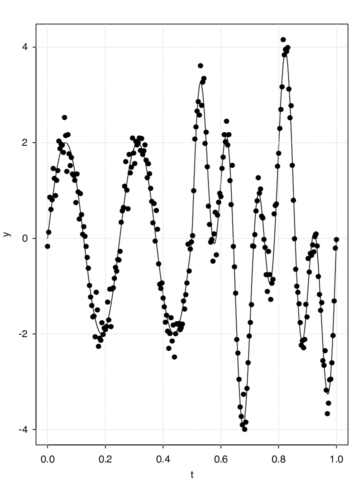
To identify frequency behaviour from the wavelet output we can calculate the discrete wavelet transform. However, because the wavelets represent variation at different discrete frequencies, we cannot obtain exact frequency values for each species at a particular time. Instead, we can calculate approximate windows of the frequency value and show how these change over time. As an example, Figure 2 (left panel) shows a time series which exhibits seasonality at different scales over different time periods. The data are simulated from:
where , , and . The right panel of Figure 2 shows its associated wavelet transform using the Daubechies’ Least Asymmetric basis. In comparison with Figure 1 (which shows the unweighted wavelet bases) we can see the transition from one level of detail (level 2 to level 3 at approx ). The frequency values for these detail levels are 4 and 8 respectively, which are not identical to above but do give an approximation to the dynamic seasonality and allow us to determine the time at which frequencies might be changing.
 |
 |
3 Modelling of multinomial data via nested ZaNI-binomial distributions
The usual probability distribution used for constrained counts across multiple categories is the multinomial. However, this distribution can be restrictive when used with the common Dirichlet conjugate prior, as has long been known [1]. Alternative link functions for the vector of proportions which aim to provide a richer set of behaviour for covariances between proportions have been proposed, for example the Isometric Log-Ratio [9, 22, ILR;] and the centralised log-ratio [23, CLR; also known as the multinomial-logistic], though these too often have restrictions on the behaviour they can model and computational restrictions come into play when the number of categories is large. Other authors have avoided transformations and used richer distributions on the simplex [23, e.g.].
An alternative approach, which remains computationally efficient even for large numbers of categories, is to decompose the count vector into nested partitions and use binomial (or binomial-like) distributions to model each section of the nesting independently. This decomposition may be identified either automatically or using informative prior information about the categories in question. In our case study we use the latter. This is related to the idea behind the nested Dirichlet distribution [21, e.g.]. However, the nested Dirichlet does not take account of the zero and inflation that arises here.
We restrict our nesting structures to binary splits only, though multiple splits are also possible [24]. We write the nesting structure as where each defines a two-component partition of the data (or a subset of it) at that particular branch of the nesting structure. Note that the order of the nesting structure is irrelevant, since each sub-model is conditionally independent. An example nesting structure for our case study is shown in Figure 4.
For a given nesting structure , vector of counts with restriction we write:
| (3.1) |
where are the probabilities associated with that branch of the nesting structure. When fitted this way, each component of the product defines an individual likelihood which, when combined with suitable prior distributions, factorises over each branch of the nesting structure. Perhaps the obvious choice for above is the binomial, but we have found this to perform poorly due to zero inflation in one or both of the counts. To account for such inflation, we use a recently proposed zero and -inflated Binomial distribution.
We consider each of our nested counts to arise from a zero inflated Poisson (ZIP) distribution [18] with some rate and zero inflation parameter. To simplify notation we consider and to arise from ZIP models, and to be their sum. We require the distribution which will naturally contain more 0 or values than expected by the standard binomial. A recently proposed distribution [28] provides for a very neat formulation via a class of Zero and inflated (ZaNI) binomials.
Perhaps the first model for zero-inflated restricted sum data was that proposed by [13]. Here a zero-inflated binomial was suggested of the form:
where is the zero-inflation parameter. However, as noted by [29], this distribution has an inconsistency in that different inferences will obtained if and are swapped, and that it is inappropriate when both counts are zero-inflated. The specific parameterisation when is a constant also does not arise naturally from the underlying ZIP models. An elegant alternative, provided by [28] sets:
where
This distribution arises naturally from the constrained zero-inflated Poisson distribution and involves positive, real-valued hyper-parameters and which control zero and inflation respectively. Now when , and when , , thus large values of indicate high levels of zero inflation and similarly high values indicate high levels of inflation. We further justify our choice of this model for our data in Section 5.
4 Data
We use data from the Irish discards sampling programme which places observers onboard demersal fishing vessels to collect discard samples. Specifically, we use the number of fish from each species discarded per haul (number of hauls=680) from 1996 until the end of 2009 in the Irish Sea. Since the sampling targets are set by quarter, the data were collated to this time unit which spanned 56 quarters.
Almost 80 species were discarded in the Irish Sea during the 14 year time-series investigated. For our model, we use seven commercial and non-commercial species. These are: whiting Merlangius merlangus, haddock Melanogrammus aeglefinus, dab Limanda limanda, plaice Pleuronectes platessa, grey gurnard Eutrigla gurnardus, norway pout Trisopterus esmarkii and poor cod Trisopterus minutus. These seven constitute 85% of all fish discarded in the Irish Sea. We aggregate the remaining 15%, which also include some commercially important species such as cod (Gadus morhua), under the label of ‘other species’. Plots of the empirical proportion () for the two most abundant species are shown in Figure 3.
 |
 |
The temporal dynamics of discards depend on the characteristics of the fishery, the environment and the biology of the species. [33] used univariate time series to show that there are annual cycles (i.e. 4 quarters) in cod, haddock and whiting discards of the Irish Sea likely owing to the seasonality in the spawning behaviour of the species. However, their model used a rigid Fourier basis. We therefore seek to determine whether these species are governed by similar dynamics in a more flexible modelling environment. We would like the model to identify these frequencies, whilst allowing for non-seasonal behaviour during certain time periods for certain species.
We use a nesting structure (Figure 4) that takes into account the classification and size of the fish involved in our study. They are separated at the first level as being either ‘abundant’ or ‘other species’, then at lower levels according to being in the familyPleuronectidae (right-eye flounders), or the order Gadiformes (ray-finned). The nesting structure we use defines seven separate models which use the counts at various levels of aggregation as detailed in Figure 4.
As we progress up the nesting structure, the likelihood of zero and inflation increases. A plot of the comparison of the aggregate Gadiformes vs non-Gadiformes (Figure 5) shows that 10% of the data are either or zero. This is because species 1 and 2 (haddock and whiting) are the most abundant of all species and thus take up all of the proportion in many cases. We might expect values of or for these models to be high.

5 Bayesian Models
In this section we outline the notation and model structure for five competing models which we later compare using WAIC [35] and out-of-sample evaluation. The models we compare are:
- 1.
A multinomial wavelet model
- 2.
A nested binomial model with constant mean
- 3.
A nested binomial wavelet model
- 4.
A nested ZI-binomial wavelet model
- 5.
A nested ZaNI-binomial wavelet model
The wavelet structures used are those outlined in Section 2. The nesting structure used is that defined in Figure 4. We include a binomial with constant mean to detect for possible Slutsky effects [25] where irregular seasonality can be spuriously obtained from smoothing. Below we provide notation for the most general case (multinomial wavelet) which can then be simplified for the other three models.
5.1 Notation
- •
is a count of fish species on trip , observation at time . is the -vector of counts for species . In total we have counts for each species.
- •
is the total number of all fish species on trip , observation at time .
- •
are zero/ inflation parameters associated with species respectively.
- •
is the proportion of fish species on trip , observation at time .
- •
is the mean proportion (logit scale) for species at time . is a -vector of means for species .
- •
is the indicator matrix which maps each mean on to a time point associated with .
- •
is the random effect for trip on species with associated variance .
- •
is the over-dispersion variance associated with proportion
- •
is a spline interpolating matrix of dimension by where is the number of wavelet basis functions and is the number of wavelet detail levels.
- •
is a wavelet basis function matrix of dimension by .
- •
is the weight coefficient associated with species and wavelet basis function . is the -vector of wavelet basis function coefficients.
- •
is a global shrinkage parameter for .
- •
is a cumulative local shrinkage parameter associated with the detail of wavelet basis function , denoted , for species .
- •
is a local shrinkage parameter associated with the detail of wavelet basis function and species .
- •
are hyper-parameters associated with the local shrinkage.
- •
is a hyper-parameter associated with global shrinkage. We fix this value.
In general we write, e.g. , to denote the entire collection of values, and similarly with other parameters. Below we outline the model structure which uses these parameters.
5.2 Model structure
Our first model sets as a multinomial-logistic distribution, and thus involves no nesting structure. The goal is to find the posterior distribution of parameters given data and . Of main interest are parameters (the species proportions), (the temporal mean dynamics), and (the wavelet coefficients). Written out in full, we have:
| (5.1) | ||||
The individual distributions are:
We outline prior distributions for the remaining terms below.
For the nested binomial, ZI-binomial and ZaNI-binomial, we introduce the given nesting structure which defines pairs formed as aggregates of the individual counts. For example, for the second layer of the nesting structure given in Figure 4 split by Gadiformes vs non-Gadiformes, and . Under this formulation, Equation 5.1 factorises over each nesting partition and thus each pair becomes a separate model. This greatly speeds up model fitting, and we now use the logit transformation rather than the multinomial-logit.
For the binomial models at nesting level we have:
For the constant mean binomial version we set all so only the random effect and over-dispersion parameters remain. For the ZI-binomial
where ZI-binomial is defined in Equation 3 and . Finally, for the ZaNI-binomial we have:
where the ZaNI-binomial is as defined in Equation 3 with and . Aside from the factorisation over and the addition of prior distributions for and , the posterior is identical to Equation 5.1.
We place weakly informative prior distributions on the remaining hyper-parameters, with the exception of , for which we follow [3] and set at . Experimentation indicates that the model is not sensitive to this setting. Overall:
- •
- •
- •
- •
- •
- •
- •
A DAG for our ZaNI-binomial model is shown in Figure 6.
6 Model fitting and results
Prior to fitting, we wrap the edges of the data to avoid edge effects. All models are fitted using STAN v2.3 [27] using the No-U-Turn sampler [14, NUTS, ], a variant of Hamiltonian Monte Carlo in which all parameters are updated simultaneously using the gradient information in the un-normalised posterior. The idea behind NUTS is that it avoids the need to tune the number of steps and the step size, which can often cause deterioration of the model output.
Using STAN, we run each of the models for 2000 iterations (1000 burn-in, no thinning) with 3 chains and check convergence using the R-hat measure [7, 12]. All of our model runs converged after this length of time. All models were fitted on a 2.6GHz Core i7 processor with 16Gb RAM. The multinomial model was slower, taking 2 hours to run. The binomials models however, could be fitted in 20 minutes for all runs of the nesting level. This could be further reduced through parallelisation, though we do not use this here as we found convergence was improved when using the values of the simpler model run as starting values for a more complex model.
For each model we compute the Wanatabe Akaike Information Criterion [35, WAIC; ]. Like other information criteria, the WAIC aims to estimate the degree to which the model fit underestimates model error. The WAIC differs from others in that it is fully Bayesian unlike, say, the deviance information criterion. In particular the WAIC penalises the deviance by a measure based on the sum of the variances of the log density, which is estimated from the posterior samples. We use:
where is the estimated log predictive density, defined as
where denotes the total number of posterior samples and denotes a posterior draw. The penalty is a measure of the effective number of parameters and is defined as the sum of the sample variances of the log density across the parameters:
where indicates the mean with respect to the posterior samples. This penalty tends to be more stable than that suggested by DIC and, by definition, guarantees a positive value for the effective number of parameters.
As an alternative measure of model fit, we also create a 10% holdout data set and test predictive performance of the models. Despite WAIC also aiming to estimate the out-of-sample fit of these models, we follow [32] in our belief that these answer differing questions about the models based on both finite and asymptotic behaviour. To make things slightly simpler, the hold-out set we create is only sampled from time points where we have multiple observations, as this means that will have already been created as part of the model run.
We first consider model comparison via WAIC. We fit the wavelet multinomial-logit, nested constant mean binomial, nested wavelet binomial, nested wavelet ZI-binomial, and nested wavelet ZaNI-binomial model to the full data set, and create WAIC values using code provided in [32]. Since WAIC is calculated on the deviance scale, we can add values provided by each nested-model and compare both multinomial and binomial models. The values are shown in Table 1. We can conclude from the totals that the nesting and the zero and inflation are beneficial over the multinomial. Furthermore, since all the binomial models are fitted on the same nesting structure we can look at the WAIC for each nested model. We note that the ZaNI-binomial is competitive for all models and seems more appropriate at more aggregated levels of the nesting structure. This is to be expected as zero and inflation is likely to be higher here.
| Nested Model | CM-B | W-B | W-ZI-B | W-ZaNI-B | Multinomial |
|---|---|---|---|---|---|
| Whiting vs Haddock | 6181 | 6172 | 6177 | 6158 | - |
| Pout vs Poor cod | 2865 | 2865 | 2877 | 2890 | - |
| Dab vs Plaice | 4172 | 4169 | 4185 | 4205 | - |
| Large vs small | 6549 | 6549 | 6533 | 6456 | - |
| Pleuronectidae vs non-Pleuronectidae | 5609 | 5620 | 5616 | 5600 | - |
| Gadiformes vs non-Gadiformes | 8266 | 8273 | 8241 | 8203 | - |
| Abundant vs Others | 8944 | 8950 | 8948 | 8913 | - |
| Total | 42586 | 42598 | 42577 | 42425 | 42960 |
Taking the ZaNI-binomial model as the chosen model, Figure 7 shows fitted values for all models. Figure 8 shows the associated wavelet transforms. We can identify some seasonal behaviour at detail level 2 in Whiting vs Haddock, detail level 4 in Dab vs Plaice (after quarter 37), and detail level 3 in Pleuronectidae vs non-Pleuronectidae and Gadiformes vs non-Gadiformes. Detail level 4 corresponds most closely with yearly periodicity whilst detail level 3 corresponds to bi-yearly seasonality.
As a final test, we use a 10% holdout data set to confirm that the ZaNI is a reasonable fit for out-of-sample data. For this test we do not use the random effects but predict from the values of . Figure 9 shows the fitted vs posterior predicted values for each of the nesting models. The fit seems very good in all models but that of Pout vs Poor Cod which is notably the model for which there is the least evidence for the wavelet ZaNI-binomial (Table 1).
 |
 |
 |
 |
 |
 |
 |
 |
 |
 |
 |
 |
 |
 |
 |
 |
 |
 |
 |
 |
 |
7 Discussion
In this paper we have proposed and fitted a novel nested wavelet zero and -inflated binomial model. The wavelet structure allows us to combine smoothing and frequency identification by using the wavelet transform. We have also used a novel shrinkage prior that has not been previously used in the wavelet literature. The nesting structure provides informative prior information on the important components of the data, and bypasses the slower and less informative traditional multinomial logit model. The performance of this model on these data seems acceptable, with the wavelet ZaNI-binomial being chosen most often via information criteria, and the out-of-sample fits showing good agreement with the left out data values.
At higher levels of the nesting structure (i.e. taxonomic order), we identified bi-yearly cycles of Gadiformes and Pleuronectidae which are likely to be a reflection of shifting fishing strategies and/or biological drivers such as spawning aggregations. For example, although most species spawn every year, certain year classes have a stronger recruitment and survival. Given that the majority of commercial species discards in the Irish Sea are from fish below the legal minimum landing size [5], the patterns observed could therefore be indicative of such phenomena in that a strong year class of Gadiformes occurs every other year.
Annual fishing regulations such as quotas and seasonal closures (i.e. cod ÔboxÕ implemented in the Irish Sea around 2000 [17]), together with fish biology such as annual recruitment, could explain the annual cycles identified at the lower levels of the nested structure, for dab and plaice. [33] identified both seasonal (year) cycles and long-term cycles for whiting and haddock discards in the Irish Sea. Although here we do not detect the annual cycles for these species, our estimate of 4 year cycles between haddock and whiting is consistent with [33] that found a mean long-term cycle of 18 quarters for haddock and 25 for whiting, possibly representing recruitment pulses of these species.
Various improvements to the model seem appropriate. First, the wavelet basis functions do not provide exact estimates of frequency. This is the price we pay for having such flexible basis functions which can be fitted to data so easily. It may be that a different choice of basis functions may provide for better frequency identification. Second, the nesting structure we have used, whilst informed by the species relationships of the fish, may instead be learnt from the data. This seems somewhat similar to the process of learning a graphical model structure [37]. It may also be that other nesting structures of which we are not aware may fit the data better. Finally, the nesting structure does not provide for frequency identification of all individual species. It is quite simple to create estimates of the posterior proportion from simple transformations of the , but this does not allow for wavelet transforms on all the individual species.
Acknowledgements
The authors would like to thank James Sweeney and John Haslett for helpful discussions on the ZaNI-binomial distribution, and Claire Gormley for drawing our attention to the wavelet shrinkage prior. This work was partly supported by the Marine Research Sub-Programme of the Irish National Development Plan 2007 – 2013 (grant PhD/FS/08/001).
5
References
- [1] Aitchison, J. (1986). The Statistical Analysis of Compositional Data. Chapman & Hall, Ltd., London, UK.
- [2] Alverson, D. L., Freeberg, M. H., Pope, J. G., and Murawski, S. A. (1994). A global assessment of fisheries bycatch and discards. Number 339 in FAO Fisheries Technical Paper. FAO. http://www.fao.org/docrep/003/t4890e/t4890e00.htm.
- [3] Bhattacharya, A. and Dunson, D. B. (2011). Sparse Bayesian infinite factor models. Biometrika 98, 2, 291–306.
- [4] Bildik, R. (2001). Intra-day seasonalities on stock returns: Evidence from the Turkish Stock Market. Emerging Markets Review 2, 4, 387–417.
- [5] Borges, L., Rogan, E., and Officer, R. (2005). Discarding by the demersal fishery in the waters around Ireland. Fisheries Research 76, 1, 1–13.
- [6] Box, G. E. P., Jenkins, G. M., and Reinsel, G. C. (2008). Time Series Analysis: Forecasting and Control, 4th ed. Wiley, London.
- [7] Brooks, S. P. and Gelman, A. (1998). General methods for monitoring convergence of iterative simulations. Journal of Computational and Graphical Statistics 7, 434–455.
- [8] Clucas, I. (1997). A Study of the Options for Utilization of Bycatch and Discards from marine capture Fisheries. FAO Fisheries Circular 928 FIIU/C, 1–59.
- [9] Egozcue, J., Pawlowsky-Glahn, V., Mateu-Figueras, G., and Barceló-Vidal, C. (2003). Isometric log-ratio transformations for compositional data analysis. Mathematical Geology 35, 3, 279–300.
- [10] European Commission. (2011). Impact Assessment of Discard Reducing Policies. Tech. rep., European Commission. http://ec.europa.eu/fisheries/documentation/studies/discards/report_en.pdf.
- [11] Franses, P. H. and Paap, R. (2004). Periodic Time Series Models. Oxford University Press, Oxford.
- [12] Gelman, A. and Rubin, D. B. (1992). Inference from iterative simulation using multiple sequences. Statistical Science 2, 457–472.
- [13] Hall, D. B. (2000). Zero-inflated Poisson and binomial regression with random effects: a case study. Biometrics 56, 4, 1030–1039.
- [14] Hoffman, M. and Gelman, A. (2011). The No-U-Turn Sampler: Adaptively Setting Path Lengths in Hamiltonian Monte Carlo. Journal of Machine Learning Research.
- [15] Holt, C. C. (2004). Forecasting seasonals and trends by exponentially weighted moving averages. International Journal of Forecasting 20, 1, 5–10.
- [16] Kelleher, K. (2005). Discards in the world’s marine fisheries. An update. FAO Fisheries Technical Paper. Rome, FAO 470, 131p.
- [17] Kelly, C. J., Codling, E. A., and Rogan, E. (2006). The Irish Sea cod recovery plan: some lessons learned. ICES Journal of Marine Science 63, 4, 600–610.
- [18] Lambert, D. (1992). Zero-Inflated Poisson Regression, with an Application to Defects in Manufacturing. Technometrics 34, 1, 1–14.
- [19] Müller, P. and Vidakovic, B., Eds. (1999). Bayesian Inference in Wavelet-Based Models. Springer.
- [20] Nason, G. P. (2008). Wavelet Methods in Statistics with R. Vol. 126. Springer.
- [21] Ng, K. W., Tang, M. L., Tan, M., and Tian, G. L. (2008). Grouped Dirichlet distribution: A new tool for incomplete categorical data analysis. Journal of Multivariate Analysis 99, 3, 490–509.
- [22] Parnell, A. C., Phillips, D. L., Bearhop, S., Semmens, B. X., Ward, E. J., Moore, J. W., Jackson, A. L., Grey, J., Kelly, D. J., and Inger, R. (2013). Bayesian stable isotope mixing models. Environmetrics 24, 6, 387–399. http://doi.wiley.com/10.1002/env.2221.
- [23] Pawlowsky-Glahn, V. and Buccianti, A. (2011). Compositional Data Analysis: Theory and Applications. Wiley-Blackwell.
- [24] Salter-Townshend, M. and Haslett, J. (2012). Fast inversion of a flexible regression model for multivariate pollen counts data. Environmetrics 23, 7, 595–605.
- [25] Slutzky, E. (1937). The summation of random causes as the source of cyclic processes. Econometrica: Journal of the Econometric Society.
- [26] So, M. K. P. and Chung, R. S. W. (2014). Dynamic seasonality in time series. Computational Statistics and Data Analysis 70, 212–226.
- [27] Stan Development Team. (2014). RStan: the R interface to Stan, Version 2.3. http://mc-stan.org.
- [28] Sweeney, J. (2012). Advances in Bayesian Model Development and Inversion in Multivariate Inverse Inference Problems with application to palaeoclimate reconstruction. Ph.D. thesis, Trinity College Dublin.
- [29] Sweeney, J. and Haslett, J. (2014). A modified Binomial likelihood model for zero/n-inflated count data. http://arxiv.org/abs/1407.0064.
- [30] Tsagarakis, K., Machias, A., Giannoulaki, M., Somarakis, S., and Karakassis, I. (2008). Seasonal and temporal trends in metrics of fish community for otter-trawl discards in a Mediterranean ecosystem. ICES Journal of Marine Science 65, 4, 539–550.
- [31] Van Opzeeland, I. C., Corkeron, P. J., Leyssen, T., Similä, T., and Van Parijs, S. M. (2005). Acoustic Behaviour of Norwegian Killer Whales, ¡I¿Orcinus orca¡/I¿, During Carousel and Seiner Foraging on Spring-Spawning Herring.
- [32] Vehtari, A. and Gelman, A. (2014). WAIC and cross-validation in Stan.
- [33] Viana, M., Jackson, A. L., Graham, N., and Parnell, A. C. (2012). Disentangling spatio-temporal processes in a hierarchical system: a case study in fisheries discards. Ecography 36, 5 (Nov.), 569–578.
- [34] Votier, S. C., Furness, R. W., Bearhop, S., Crane, J. E., Caldow, R. W. G., Catry, P., Ensor, K., Hamer, K. C., Hudson, A. V., Kalmbach, E., Klomp, N. I., Pfeiffer, S., Phillips, R. A., Prieto, I., and Thompson, D. R. (2004). Changes in fisheries discard rates and seabird communities. Nature 427, 6976, 727–730.
- [35] Watanabe, S. (2013). A Widely Applicable Bayesian Information Criterion. Machine Learning Research 14, 1, 867–897.
- [36] Winters, P. R. (1960). Forecasting Sales by Exponentially Weighted Moving Averages. Management Science 6, 3 (Apr.), 324–342.
- [37] Yuan, M. and Lin, Y. (2007). Model selection and estimation in the Gaussian graphical model. Biometrika.