Symmetry reduction of holomorphic iterated function schemes and factorization of Selberg zeta functions

David Borthwick Affiliation: Dept of Math/CS, Emory University Atlanta, GA 30322, USA Tobias Weich ^†^†thanks: weich@math.uni-paderborn.de Affiliation: Institut für Mathematik, Universität Paderborn,33098 Paderborn, Germany

Abstract

Given a holomorphic iterated function scheme with a finite symmetry group $G$ , we show that the associated dynamical zeta function factorizes into symmetry-reduced analytic zeta functions that are parametrized by the unitary irreducible representations of $G$ . We show that this factorization implies a factorization of the Selberg zeta function on symmetric $n$ -funneled surfaces and that the symmetry factorization simplifies the numerical calculations of the resonances by several orders of magnitude. As an application this allows us to provide a detailed study of the spectral gap and we observe for the first time the existence of a macroscopic spectral gap on Schottky surfaces.

1 Introduction

Let $X=\Gamma\backslash\mathbb{H}$ be a convex co-compact hyperbolic surface, with $\Delta_{X}$ the positive Laplacian on this surface. The resolvent, written in the form

R(s)=(\Delta_{X}-s(1-s))^{-1},

(1.1)

is analytic as an operator on $L^{2}(X)$ for $s\in\mathbb{C}$ with $\operatorname{Re}(s)>1$ . As an operator on weighted function spaces it can be continued meromorphically to $s\in\mathbb{C}$ with poles of finite rank [21]. The poles of this meromorphic continuation are called the resonances of $X$ and the multiplicity of a resonance is defined to be the rank of the associated pole. The set of all resonances on $X$ , repeated according to multiplicity, will be called $\textup{Res}(X)$ . The resonance set is the spectral invariant of the surface $X$ which generalizes the discrete eigenvalue spectrum of the Laplacian on a compact manifold.

Interest in the distribution of the resonances arises from different areas of research. First it is a natural mathematical question to understand the strength of the relationship between the geometry of the surface $X$ and the distribution of resonances. Second, the distribution of resonances on infinite volume hyperbolic surfaces has been found to have implications in arithmetics [7]. And third, the Laplace operator on convex co-compact surfaces is an important model for quantum-chaotic scattering, and the resonance distribution has been intensively studied in theoretical [32, 20] and experimental [3, 29] physics during recent years.

With motivation coming from these different directions, various results on the distribution of resonances on convex co-compact surfaces have been obtained. These include, for example, results on the asymptotic number of resonances in a disk in the complex plane [13, 14, 5], results on upper and lower bounds of resonances in a strip near the critical line [36, 12, 28, 15, 23] and about asymptotic spectral gaps [22, 16] in the limit of large $\operatorname{Im}(s)$ . Despite these big advances, there are still many open conjectures on the distribution of the resonances, for example the fractal Weyl upper bound is conjectured to be sharp [12] and the asymptotic spectral gap is conjectured to be much bigger then what is actually known [17]. We refer to [24] for a more detailed overview on recent results and open questions.

In order to test these conjectures numerically, the first author recently presented a detailed numerical study of the resonance structure on convex co-compact surfaces [6]. Those calculations exploit the fact that the resonances appear as zeros of the Selberg zeta function. This zeta function is defined for $\operatorname{Re}(s)>1$ by

Z_{X}(s):=\prod\limits_{\gamma\in\mathcal{P}_{X}}\prod\limits_{k\geq 0}\left(1-e^{-(s+k)l(\gamma)}\right),

(1.2)

where $\mathcal{P}_{X}$ is the set of primitive closed geodesics on $X$ (those geodesics that cannot be obtained by a repetition of a shorter closed geodesic) and $l(\gamma)$ denotes the length. For convex co-compact surfaces the Selberg zeta function is known to extend analytically to the complex plane [11] and the relation to the resonances of $\Delta_{X}$ is given by the following:

Theorem 1.1 ([27] Patterson-Perry 2001).

For a convex co-compact surface $X=\Gamma\backslash\mathbb{H}$ the zero set of the zeta function $Z_{X}(s)$ is the union of the resonances $\textup{Res}(X)$ and the negative integers $s=-k$ , $k\in\mathbb{N}_{0}$ .

For an tractable numerical calculation of the Selberg zeta function, the correspondence of the Selberg zeta function and the dynamical zeta function of an iterated function scheme, the Bowen-Series map, has been used. The problem of analytic continuation can be circumvented by a trick which was introduced under the name cycle expansion in physics [9] by Cvitanovic-Eckhardt and which has later been rigorously applied to Selberg zeta functions by Jenkinson-Pollicott [18]. These techniques allow the calculation of several thousand resonances on an ordinary personal computer and make it possible to study their distribution in the complex plane. By this approach, in [6] resonance distributions were compared to the existent conjectures. Those investigations also revealed the striking formation of resonance chains, which triggered further numerical [2, 35] and mathematical [34] studies.

The problem with the numerical techniques used so far is that, due to the exponential growth of number of closed geodesics, the convergence of the algorithm is restricted to rather narrow resonance strips near the critical line. Additionally, only surfaces whose Schottky groups have two generators and for which the fractal dimension of the limit set $\delta$ is rather small ( $0\leq\delta\lesssim 0.1$ ) could be treated [6, Section 4.1]. For a more thorough tests of the conjectures a larger $\delta$ -range would be desirable. Furthermore, recent predictions that the resonance chains observed for 3-funneled surface should be much less clear for 4-funneled surfaces [2] can not be tested at all with the current techniques.

These shortcomings of the existent techniques motivated us to take advantage of the symmetry of the convex co-compact surfaces and prove a symmetry factorization for the dynamical zeta functions. Such factorizations have been calculated in physics in the closely related setting of $3$ - and $4$ -disk systems by Cvitanovic and Eckhardt [10]. The aim of this article is to establish rigorous version of their results and apply them to the calculation of resonances on convex co-compact surfaces.

If a convex co-compact surface $X=\Gamma\backslash\mathbb{H}$ has a finite symmetry group $G$ , then the natural approach for a symmetry-reduced calculation of the resonances would be to apply the symmetry reduction on the level of the Laplacian $\Delta_{X}$ and to study the meromorphic continuation of the symmetry-reduced resolvent. For the numerical calculation of the resonances we need, however, the Patterson-Perry correspondence (Theorem 1.1). The proof of a factorization of the Selberg zeta function thus would require to reprove this correspondence for the symmetry-reduced resolvent, which seems rather technical. Therefore we have chosen to prove the factorization on the level of the dynamical zeta functions of iterated function schemes. This approach has the advantage that the results apply not only to Bowen-Series maps and convex co-compact surfaces but also extend immediately to other cases where iterated function schemes appear, e.g., in the calculation of Hausdorff dimensions [18]. Additionally, one automatically obtains the analyticity of the symmetry-reduced zeta functions for free. The drawback of this approach is, however, that the symmetry group of the commonly used Bowen-Series maps might be smaller then the symmetry group of the associated surface. This problem can be circumvented for a large class of interesting surfaces as we will show in Section 5.1.

The article is organized as follows. In Section 2 we will first introduce the holomorphic iterated function schemes (IFS), their transfer operators and the dynamical zeta functions. In Section 3 we will introduce the notion of a symmetry group of a holomorphic IFS and derive a symmetry-reduced trace formula for the transfer operator (Proposition 3.3). This symmetry-reduced trace formula is then used in Section 4 to prove, as a first main result, the factorization of the dynamical zeta function (Theorem 4.6). The rest of the section is devoted to a simplification of the symmetry-reduced zeta functions (Theorem 4.6 and Corollary 4.8) which hold under the assumption that the symmetry group acts freely on the set of $G$ -closed words.

Section 5 is then devoted to the application of the results to the resonances on convex co-compact surfaces. In Section 5.1 we first introduce a family of symmetric $n$ -funneled surfaces for which we construct iterated function schemes that incorporate the whole symmetry group of the surfaces. Using Theorem 4.1, this leads to a factorization of the Selberg zeta function into analytic symmetry-reduced zeta functions (see equation (5.9)). Finally, in Section 5.2, we perform the numerical calculations using these new symmetry-reduced formulas. The symmetry reduction is interesting for theoretical reasons as it allows to associate the calculated resonances to particular unitary irreducible representations of the symmetry group. We also demonstrate the tremendous practical value of the symmetry reduction as a means of simplifying the numerical calculations: For a 3-funneled surface we show that we can increase the width of the numerically accessible resonance strip by a factor of three and at the same time reduce the number or required periodic orbits from over 170 000 without symmetry reduction to only 41 with symmetry reduction. We are confident that this gain of efficiency will allow much more thorough numerical investigations of the resonance structure on convex co-compact surfaces. As first examples of this, we confirm the prediction from [2] that the resonance structure of symmetric 4-funneled surfaces show no clearly visible resonance chains. We also provide a detailed study of the spectral gap on Schottky surface and observe for the first time the existence of a macroscopic spectral gap on these surfaces.

Acknowledgments: T.W. has been suported by the German Research Foundation (DFG) via the grant DFG HI 412/12-1. This work was initiated at the conference on “Quantum chaos, resonances, and semiclassical measures”, Roscoff, France, June 2013, sponsored by a grant from the ANR.

2 Holomorphic iterated function schemes and their transfer operators

Definition 2.1.

A holomorphic iterated function scheme (IFS) is defined on a set of $N$ open disks $D_{1},\dots,D_{N}\subset\mathbb{C}$ whose closures $\overline{D}_{i}$ are pairwise disjoint. Associated to the IFS is a matrix $A\in\{0,1\}^{N\times N}$ called the adjacency matrix, which defines a relation $i\rightsquigarrow j$ if $A_{i,j}=1$ . It is assumed that for each pair $(i,j)\in\{1,\dots,N\}^{2}$ with $i\rightsquigarrow j$ we have a biholomorphic map $\phi_{i,j}:D_{i}\to\phi_{i,j}(D_{i})\Subset D_{j}$ . The images are required to be pairwise disjoint in the sense that

\phi_{i,j}(D_{i})\cap\phi_{k,l}(D_{k})\neq\emptyset\quad\Longleftrightarrow\quad(i,j)=(k,l).

(2.1)

For convenience we denote the union of all the disjoint disks by

D:=\bigcup_{i}D_{i}

and the union of all their images by

\phi(D):=\bigcup\limits_{i\rightsquigarrow j}\phi_{i,j}(D_{i}).

From (2.1) it follows directly that for $u\in\phi(D)$ there is exactly one pair $i\rightsquigarrow j$ and a unique $u^{\prime}\in D_{i}$ such that $u=\phi_{i,j}(u^{\prime})$ . We have thus a well defined holomorphic inverse function

\phi^{-1}:\phi(D)\to D.

Remark 2.2.

Instead of disks $D_{i}$ one could have also taken simply connected domains $U_{i}\subset\mathbb{C}$ . Using the Riemann mapping theorem such an IFS is biholomorphically conjugate to an IFS with disks, so one can always simplify such an IFS to the above situation defined on disks.

Example 2.3.

Let $D_{1},\dots,D_{2r}$ be disjoint open disks in $\mathbb{C}$ with centers on the real line and mutually disjoint closures. Then there exists for each pair $D_{i},D_{i+r}$ an element $S_{i}\in PSL(2,\mathbb{R})$ that maps via its Moebius transformation $\partial D_{i}$ to $\partial D_{i+r}$ and that maps the interior of $D_{i}$ to the exterior of $D_{i+r}$ . The Schottky group is then the free subgroup $\Gamma\subset PSL(2,\mathbb{R})$ , generated by $S_{1},\dots,S_{r}$ (for an illustration see Figure 1). The quotient $\Gamma\backslash\mathbb{H}$ is a hyperbolic surface with Euler characteristic $\chi=1-r$ , and any convex co-compact hyperbolic surface admits such a representation [8].

The generators and disks in the construction of a Schottky group give also a natural construction of a holomorphic IFS. For convenience we write $S_{i+r}:=S_{i}^{-1}$ for $i=1,\dots,r$ and use a cyclic notation of the indices: $S_{i+2r}:=S_{i}$ and $D_{i+2r}:=D_{i}$ . Then for all $i=1,\dots,2r$ the element $S_{i}$ maps all disks except $D_{i}$ holomorphically into the interior of $D_{i+r}$ . The adjacency matrix of this IFS is thus the $2r\times 2r$ matrix with $A_{i,j}=0$ if $|i-j|=r$ and $A_{i,j}=1$ else. Furthermore for any $i\rightsquigarrow j$ we define the maps for $u\in D_{i}$ by

\phi_{i,j}(u):=S_{j+r}u=S_{j}^{-1}u\in D_{j},

and from this definition it is clear that (2.1) is automatically fulfilled.

Note that the inverse map restricted to $D_{j}\cap\phi(D)$ is exactly given by $S_{j}$ . The IFS which we defined is consequently the inverse of the usual Bowen-Series map for Schottky groups (see e.g. [4, Section 15.2]).

Refer to caption — Figure 1: Illustration of the construction of a Schottky group and the corresponding IFS. The blue disks show the four disks from which the generators of the Schottky group are generated. For example the group element $S_{1}$ maps $\partial D_{1}$ to $\partial D_{3}$ and the exterior of $D_{1}$ into the interior of $D_{3}$ . The red circles illustrate the images of the other three disks under the Moebius transformation $S_{1}$ which coincide with the images of the disks under the associates holomorphic IFS.

Returning to the general case with $N$ disks, it will turn out to be useful for the notation to introduce the following symbolic coding. The symbols are given by the integers $1,\dots,N$ and the set of words of length $n$ is given by the tuples of symbols

\mathcal{W}_{n}:=\{(w_{0},\dots,w_{n}):\>w_{i}\rightsquigarrow w_{i+1}\textup{ for all }i=0,\dots,n-1\}.

Note that our notation of word length does not refer to the number of symbols, but to the number of transitions which they indicate. For $w\in\mathcal{W}_{n}$ and $0<k\leq n$ we define the truncated word by

w_{0,k}:=(w_{0},\dots,w_{k})\in\mathcal{W}_{k}.

(2.2)

Finally we define the iteration of the maps $\phi_{i,j}$ along a word $w\in\mathcal{W}_{n}$ as

\phi_{w}:=\phi_{w_{n-1},w_{n}}\circ\ldots\circ\phi_{w_{0},w_{1}}:D_{w_{0}}\mapsto D_{w_{n}}

and their images as

D_{w}:=\phi_{w}(D_{w_{0}}).

Note that $D_{w}\Subset D_{w_{n}}$ and that from the separation condition (2.1) one obtains inductively for $w,w^{\prime}\in\mathcal{W}_{n}$

D_{w}\cap D_{w^{\prime}}\neq\emptyset\quad\Longleftrightarrow\quad w=w^{\prime}.

Definition 2.4.

We call a holomorphic IFS eventually contracting if there is some $N\in\mathbb{N}$ and $\theta<1$ such that for $n\geq N$

|\phi_{w}^{\prime}(u)|\leq\theta\textup{ for all }w\in\mathcal{W}_{n}\textup{ and }u\in D_{w_{0}}.

Remark 2.5.

The Bowen-Series IFS as introduced in Example 2.3 are known to be eventually contracting (see e.g. [4, Proposition 15.4]).

We say a word $w\in\mathcal{W}_{n}$ of length $n$ is closed if $w_{0}=w_{n}$ and we denote the set of all closed words of length $n$ by $\mathcal{W}_{n}^{cl}$ .

Lemma 2.6.

If a holomorphic IFS is eventually contracting, then for each $w\in\mathcal{W}_{n}^{cl}$ there exists a unique fixed point $\phi_{w}(u_{w})=u_{w}$ .

Proof.

If $w\in\mathcal{W}_{n}^{cl}$ is closed, then $\phi_{w}(D_{w_{0}})=D_{w}\Subset D_{w_{0}}$ and we write $K_{k}:=(\phi_{w})^{k}(D_{w_{0}})$ . Then $K_{k+1}\Subset K_{k}$ and if $k_{0}n\geq N$ then from the eventually contracting property $\textup{diam}(K_{k_{0}m})\leq\theta^{m}\textup{diam}(D_{w_{0}})$ . Then $K_{1},K_{2},\ldots$ is a nested sequence of disks whose diameter converges to zero, so there is a unique $u_{w}:=\bigcap_{k>0}K_{k}$ which must be a fixed point of $\phi_{w}$ . ∎

Our next goal is to define the transfer operators associated to the iterated function schemes.

Definition 2.7 (transfer operator).

Let $\mathcal{B}(D):=\{f:D\to\mathbb{C}\textup{ holomorphic, and }f\in L^{2}(D)\}$ be the Bergmann space on $D$ , where $D:=\cup D_{i}$ for a holomoprhic IFS. For $V:\phi(D)\to\mathbb{C}$ a bounded holomorphic function, we define the transfer operator $\mathcal{L}_{V}:\mathcal{B}(D)\to\mathcal{B}(D)$ associated to the IFS by

(\mathcal{L}_{V}f)(u):=\sum\limits_{j:\>i\rightsquigarrow j}V(\phi_{i,j}(u))f(\phi_{i,j}(u)),\quad\textup{ for }u\in D_{i}.

(2.3)

Given such a potential $V$ , a word $w\in\mathcal{W}_{n}$ and a point $u\in D_{w_{0}}$ we can define the iterated product

V_{w}(u):=\prod\limits_{k=1}^{n}V(\phi_{w_{0,k}}(u)),

(2.4)

where $w_{0,k}$ is the truncation $(w_{0},\dots,w_{k})$ as defined in (2.2). A straight forward calculation of powers of the transfer operator $\mathcal{L}_{V}$ leads to

\left(\mathcal{L}_{V}^{n}f\right)(u)=\sum\limits_{w\in\mathcal{W}_{n}:\>u\in D_{w_{0}}}V_{w}(u)f(\phi_{w}(u));

thus these iterated products naturally occur in powers of $\mathcal{L}_{V}$ .

It is a well known fact that these transfer operators are trace class (see [30] for the original proof in slightly different function spaces or [4, Lemma 15.7] for a proof in our setting) and that the trace can be expressed in terms of periodic orbits. Accordingly one can define the dynamical zeta function by the Fredholm determinant

d_{V}(z):=\det(1-z\mathcal{L}_{V})

(2.5)

which is an entire function on $\mathbb{C}$ . If furthermore the IFS is eventually contracting the dynamical zeta function can be written for $|z|$ sufficiently small as (see e.g. [4, proof of Thm. 15.8]):

d_{V}(z)=\exp\left(-\sum\limits_{n>0}\frac{z^{n}}{n}\sum\limits_{w\in\mathcal{W}_{n}^{cl}}V_{w}(u_{w})\frac{1}{1-(\phi_{w})^{\prime}(u_{w})}\right).

(2.6)

Example 2.8.

An important class of transfer operators arises from the IFS associated to Bowen-Series maps of Schottky surfaces (see Example 2.3). If we choose the potential function $V_{s}(u)=[(\phi^{-1})^{\prime}(u)]^{-s}$ , which depends analytically on $s\in\mathbb{C}$ , then one obtains an analytic family of trace class operators $\mathcal{L}_{s}$ . The dynamical zeta function

d(s,z):=\det(1-z\mathcal{L}_{s})

is then analytic in $(s,z)\in\mathbb{C}^{2}$ . One has the important relation to the Selberg zeta function $Z_{X}$ for the Schottky surface $X$ ,

Z_{X}(s)=d(s,1),

where $Z_{X}(s)$ was defined in (1.2) as a product over the primitive closed geodesics (see e.g. [4, Thm. 15.8] for a proof).

3 Trace formula for the symmetry-reduced transfer operator

Definition 3.1.

A symmetry group of a holomorphic IFS is a finite group $G$ which acts holomorphically on $D$ and commutes with the IFS in the sense that for each $g\in G$ , $u\in D_{i}$ and $i\rightsquigarrow j$ , there exists a pair $k\rightsquigarrow l$ such that $g\phi_{i,j}(u)=\phi_{k,l}(gu)$ .

As an immediate consequence of the definition we obtain that $\phi(D)\subset D$ is a $G$ -invariant subset. Furthermore, as the disks $D_{i}$ are disjoint and connected, we have

g(D_{i})=D_{j}.

(3.1)

Thus we can reduce the $G$ -action to the set of symbols $\{1,\dots,N\}$ by setting $gi:=j$ for $i,j$ such that (3.1) holds. With this notation the indices $k,l$ in Definition 3.1 are uniquely defined by $k=gi$ and $l=gj$ . Accordingly we conclude that $i\rightsquigarrow j$ implies $gi\rightsquigarrow gj$ and consequently we can extend the $G$ -action on the symbols to an action on the words of length $n$ by setting for $w\in\mathcal{W}_{n}$

gw:=(gw_{0},\dots,gw_{n})\in\mathcal{W}_{n}.

For the iterated maps $\phi_{w}$ , the commutation formula reads

g\phi_{w}(u)=\phi_{gw}(gu).

(3.2)

For further use we can also introduce for $g\in G$ the set of $g$ -closed words of length $n$

\mathcal{W}_{n}^{g}:=\{w\in\mathcal{W}_{n},gw_{n}=w_{0}\}.

(3.3)

Example 3.2.

We have seen in Example 2.3 that Schottky groups naturally give rise to holomorphic IFS. We will now consider the special case of 3-funneled surfaces. These surfaces are known to be uniquely parametrized by their Fenchel-Nielsen coordinates $l_{1},l_{2},l_{3}$ which determine the lengths of the three fundamental geodesics $\gamma_{1},\gamma_{2},\gamma_{3}$ (see Figure 2).

Given three lengths $l_{1},l_{2},l_{3}$ we denote the associated Schottky surface by $X_{l_{1},l_{2},l_{3}}=\Gamma_{l_{1},l_{2},l_{3}}\backslash\mathbb{H}$ . The two generators of the Schottky group can be written in the form

S_{1}=\left(\begin{array}[]{cc}\cosh(l_{1}/2)&\sinh(l_{1}/2)\\ \sinh(l_{1}/2)&\cosh(l_{1}/2)\end{array}\right),\penalty\ \penalty\ \penalty\ S_{2}=\left(\begin{array}[]{cc}\cosh(l_{2}/2)&a\sinh(l_{2}/2)\\ a^{-1}\sinh(l_{2}/2)&\cosh(l_{2}/2)\end{array}\right),

where the parameter $a>0$ is chosen such that $\operatorname{Tr}(S_{1}S_{2}^{-1})=-2\cosh(l_{3}/2)$ .

Depending on the choice of $l_{1},l_{2},l_{3}$ the associated Bowen-Series IFS have different symmetry groups. In any case the IFS has a $\mathbb{Z}_{2}$ symmetry generated by the Moebius transformation of the matrix

\sigma_{1}=\left(\begin{array}[]{cc}-1&0\\ 0&1\end{array}\right).

This transformation corresponds to a reflection at the imaginary axis followed by a complex conjugation¹¹ 1 This complex conjugation is necessary to make the symmetry holomorphic. and it is related to the fact that all 3-funneled Schottky surfaces are symmetric with respect to reflections on the plane spanned by the three funnels.

The action of $\sigma_{1}$ interchanges disk $D_{1}$ with $D_{3}$ and $D_{2}$ which $D_{4}$ , thus we get the following action on the symbols

\sigma_{1}(1)=3,\quad\sigma_{1}(2)=4,\quad\sigma_{1}(3)=1,\quad\sigma_{1}(4)=2.

In order to prove that $\sigma_{1}$ is indeed a symmetry of the Bowen-Series IFS in the sense of Definition 3.1 we have to verify

	$\displaystyle\sigma_{1}\phi_{1,1}\sigma_{1}=\phi_{3,3},\quad\sigma_{1}\phi_{2,1}\sigma_{1}=\phi_{4,3},\quad\sigma_{1}\phi_{4,1}\sigma_{1}=\phi_{2,3}$
	$\displaystyle\sigma_{1}\phi_{1,2}\sigma_{1}=\phi_{3,4},\quad\sigma_{1}\phi_{2,2}\sigma_{1}=\phi_{4,4},\quad\sigma_{1}\phi_{3,2}\sigma_{1}=\phi_{1,4}.$

The first line follows from the fact that

\sigma_{1}S_{1}\sigma_{1}=\left(\begin{array}[]{cc}\cosh(l_{1}/2)&-\sinh(l_{1}/2)\\ -\sinh(l_{1}/2)&\cosh(l_{1}/2)\end{array}\right)=S_{1}^{-1}=S_{3}

and the second line analogously from $\sigma_{1}S_{2}\sigma_{1}=S_{4}$ .

If the Fenchel-Nielsen coordinates satisfy $l_{1}=l_{2}$ then both the Schottky surface $X_{l_{1},l_{1},l_{3}}$ and the Bowen-Series IFS admit an additional symmetry. On the surface this symmetry would correspond to a rotation of $180^{\circ}$ around the third funnel. For the IFS this symmetry is represented by a Moebius transformation of the matrix

\sigma_{2}=\left(\begin{array}[]{cc}0&\sqrt{a}\\ \frac{1}{\sqrt{a}}&0\end{array}\right).

This transformation represents a reflection at the orange circle in Figure 3 followed again by a complex conjugation to restore the holomorphicity. As this transformation interchanges $D_{1}$ with $D_{2}$ and $D_{3}$ with $D_{4}$ we obtain the action on the symbols

\sigma_{2}(1)=2,\quad\sigma_{2}(2)=1,\quad\sigma_{2}(3)=4,\quad\sigma_{2}(4)=3

and according to Definition 3.1 we have to check

	$\displaystyle\sigma_{2}\phi_{1,1}\sigma_{2}=\phi_{2,2},\quad\sigma_{2}\phi_{2,1}\sigma_{2}=\phi_{1,2},\quad\sigma_{2}\phi_{4,1}\sigma_{2}=\phi_{3,2}$
	$\displaystyle\sigma_{2}\phi_{2,3}\sigma_{2}=\phi_{1,4},\quad\sigma_{2}\phi_{3,3}\sigma_{2}=\phi_{4,4},\quad\sigma_{2}\phi_{4,3}\sigma_{2}=\phi_{3,4}.$

This is again verified by a simple matrix calculation that shows that $\sigma_{2}S_{1}\sigma_{2}=S_{2}$ and $\sigma_{2}S_{3}\sigma_{2}=S_{4}$ . Since $\sigma_{1}$ and $\sigma_{2}$ commute, we conclude that in the case $l_{1}=l_{2}$ the surface the holomorphic IFS have the Klein four-group as symmetry group.

If all three fundamental lengths are equal to each other, $l_{1}=l_{2}=l_{3}=l$ , then the Schottky surface $X_{l,l,l}$ has an even larger group as symmetry group which can be written as $\mathcal{D}_{3}\times\mathbb{Z}_{2}$ , with $\mathcal{D}_{3}$ being the symmetry group of the equilateral triangle (see Section 5.1 for more details). The Bowen-Series IFS however does not exhibit these extra symmetries and still has only the Klein four-group as symmetry group. The reason for this discrepancy lies in the construction of the Bowen-Series IFS. Morally, it corresponds to a Poincaré section which is defined by the blue dotted and red dashed cut-lines in Figure 2. This asymmetric choice of a Poincaré section is the reason why the holomorphic IFS has a weaker symmetry then the whole surface. To obtain the full symmetry decomposition of the zeta function we will have to construct a holomorphic IFS whose dynamical zeta function corresponds also to the Selberg zeta function but which incorporates the full symmetry group of the surface. This will be done for symmetric n-funneled surfaces in Section 5.1.

Given a symmetry group $G$ of a holomorphic IFS we now want to define the symmetry decomposition of the function spaces $B(D)$ . The symmetry group $G$ acts from left on $B(D)$ by its left regular representation

(gf)(u)=f(g^{-1}u).

Note that in general this action is not unitary if the scalar product in $B(D)$ is taken with respect to the Lebesgue measure. However, by averaging the Lebesgue measure $\lambda$ over $G$ with the pushforward $g_{*}\lambda$ one obtains a $G$ -invariant measure

\mu_{G}:=\frac{1}{|G|}\sum\limits_{g\in G}g_{*}\lambda=\frac{1}{|G|}\sum\limits_{g\in G}|g^{\prime}(u)|^{-1}\lambda,

which just modifies the Lebesgue measure by a positive, smooth density factor. We denote the Bergman space with the scalar product defined by $\mu_{G}$ with $B_{G}(D)$ . This space is identical to $B(D)$ as a set, but equipped with a different, topologically equivalent scalar product.

On $B_{G}(D)$ the left regular action of $G$ is unitary. We thus get a decomposition

B_{G}(D)=\bigoplus\limits_{\chi\in\hat{G}}B^{\chi}

(3.4)

where $\hat{G}$ is the set of equivalence classes of unitary representations of $G$ and $B^{\chi}:=P_{\chi}B_{G}(D)$ with the orthogonal projection operator

P_{\chi}:=\frac{d_{\chi}}{|G|}\sum\limits_{g\in G}\overline{\chi(g)}g.

Here $\chi$ is the character of the irreducible representation of dimension $d_{\chi}$ and $g$ the operator defined by the left regular representation. Note that the definition of $P_{\chi}$ does not involve the scalar product, thus the operators $P_{\chi}$ are equally projectors on $B(D)$ and we also get the decomposition of $B(D)$ in closed linear subspaces

B(D)=\bigoplus\limits_{\chi\in\hat{G}}B^{\chi}.

(3.5)

The only difference to (3.4) is that this decomposition is in general not orthogonal anymore.

If the potential $V$ of the transfer operator is $G$ -invariant, in the sense that

V(gu)=V(u),

(3.6)

then $\mathcal{L}_{V}$ commutes with the left regular representation on $B(D)$ and accordingly also with the projectors $P_{\chi}$ . Consequently $\mathcal{L}_{V}$ leaves the spaces $B^{\chi}$ invariant and we define the symmetry-reduced transfer operator to be

\mathcal{L}_{V}^{\chi}:={\mathcal{L}_{V}}\bigr|_{B^{\chi}}:B^{\chi}\to B^{\chi}.

(3.7)

For this symmetry-reduced operator we obtain the following formula for its trace:

Proposition 3.3.

Let $G$ be the symmetry group of a holomorphic, eventually contracting IFS, with $V:\phi(D)\to\mathbb{C}$ a holomorphic, bounded function which is symmetric with respect to the $G$ -action and $\mathcal{L}_{V}$ the associated transfer operator. Then for all $n\in\mathbb{N}$ , ${(\mathcal{L}_{V}^{\chi})^{n}}$ is trace class and its trace is given by:

\operatorname{Tr}_{B^{\chi}}\left[(\mathcal{L}_{V}^{\chi})^{n}\right]=\frac{d_{\chi}}{|G|}\sum\limits_{g\in G}\chi(g)\sum\limits_{w\in\mathcal{W}^{g}_{n}}\frac{V_{w}(gu_{w,g})}{1-(\phi_{w}\circ g)^{\prime}(u_{w,g})},

(3.8)

where $u_{w,g}$ is the unique fixed point satisfying

u_{w,g}=\phi_{w}(gu_{w,g}),

(3.9)

and $V_{w}$ is the iterated product

V_{w}(u)=\prod\limits_{k=1}^{n}V(\phi_{w_{0,k}}(u)).

Proof.

This proposition is a direct consequence of [4, Lemma 15.7]. First, we note that

\operatorname{Tr}_{B^{\chi}}[(\mathcal{L}_{V}^{\chi})^{n}]=\operatorname{Tr}_{B(D)}[P_{\chi}(\mathcal{L}_{V})^{n}].

Since $\overline{\chi(g)}=\chi(g^{-1})$ , we can replace $g$ by $g^{-1}$ in the definition of $P_{\chi}$ and calculate that

(P_{\chi}(\mathcal{L}_{V})^{n}f)(u)=\frac{d_{\chi}}{|G|}\sum\limits_{g\in G}\chi(g)\sum\limits_{w\in\mathcal{W}_{n}:\>gu\in D_{w_{0}}}V_{w}(gu)f(\phi_{w}(gu)).

This implies that

\operatorname{Tr}_{B^{\chi}}[(\mathcal{L}_{V}^{\chi})^{n}]=\frac{d_{\chi}}{|G|}\sum\limits_{g\in G}\chi(g)\sum\limits_{w\in\mathcal{W}_{n}:\>gu\in D_{w_{0}}}\operatorname{Tr}_{B(D)}\left[T_{V,w,g}\right]

where $T_{V,w,g}$ is the following transfer operator

(T_{V,w,g}f)(u):=\left\{\begin{array}[]{ll}V_{w}(gu)f(\phi_{w}\circ g(u))&\textup{ if }u\in D_{g^{-1}w_{0}}\\ 0&\textup{ else}\end{array}\right.

The map $\phi_{w}\circ g$ is a biholomorphic function $\phi_{w}\circ g:D_{g^{-1}w_{0}}\to D_{w}\Subset D_{w_{n}}$ . If $w_{n}\neq g^{-1}w_{0}$ , or in other words, if $w\notin\mathcal{W}^{g}_{n}$ , then the operator has trace zero as it is an isomorphism between two orthogonal subsets of $B(D)$ . Otherwise the eventually contracting property implies by the same arguments as in the proof of Lemma 2.6 that the map $\phi_{w}\circ g$ has a unique fixed point which we call $u_{w,g}$ . The operator $T_{V,w,g}$ then fulfills all the conditions of [4, Lemma 15.7] and we obtain

\operatorname{Tr}_{B(D)}(T_{V,w,g})=\frac{V_{w}(gu_{w,g})}{1-(\phi_{w}\circ g)^{\prime}(u_{w,g})}.

∎

4 Factorization of the zeta function

Proposition 3.3 allows us to prove the following factorization of the dynamical zeta function.

Theorem 4.1.

Let $G$ be the symmetry group of a holomorphic, eventually contracting IFS, let $V:\phi(D)\to\mathbb{C}$ be a holomorphic, bounded $G$ -invariant potential and $d_{V}(z)$ the dynamical zeta function associated to the IFS and $V$ . Then the dynamical zeta function admits a factorization,

d_{V}(z)=\prod\limits_{\chi\in\hat{G}}d_{V}^{\chi}(z),

where the reduced zeta functions $d_{V}^{\chi}(z)$ can be expressed for sufficiently small $|z|$ by

d_{V}^{\chi}(z)=\exp\left(-\sum\limits_{n>0}\frac{z^{n}}{n}\frac{d_{\chi}}{|G|}\sum\limits_{g\in G}\chi(g)\sum\limits_{w\in\mathcal{W}^{g}_{n}}V_{w}(gu_{w,g})\sum\limits_{k\geq 0}\left[(\phi_{w}\circ g)^{\prime}(u_{w,g})\right]^{k}\right),

(4.1)

and they extend analytically to $\mathbb{C}$ .

Proof.

As Proposition 3.3 assures that $\mathcal{L}_{V}^{\chi}$ is trace class, we can define the symmetry-reduced zeta function

d_{V}^{\chi}(z):={\det}_{B^{\chi}}(1-z\mathcal{L}_{V}^{\chi})

(4.2)

which is an analytic function on $\mathbb{C}$ . From the symmetry decomposition (3.5) of $B(D)$ into invariant subspaces $B^{\chi}$ we furthermore directly obtain the following factorization of the dynamical zeta function

d_{V}(z)=\prod\limits_{\chi\in\hat{G}}d_{V}^{\chi}(z).

Using the formula for the Fredholm determinant and the symmetry-reduced trace formula we obtain

	$\displaystyle d_{V}^{\chi}(z)$	$\displaystyle=$	$\displaystyle\exp\left(-\sum\limits_{n>0}\frac{z^{n}}{n}\operatorname{Tr}_{B^{\chi}}\left[(\mathcal{L}_{V}^{\chi})^{n}\right]\right)$
		$\displaystyle=$	$\displaystyle\exp\left(-\sum\limits_{n>0}\frac{z^{n}}{n}\frac{d_{\chi}}{\|G\|}\sum\limits_{g\in G}\chi(g)\sum\limits_{w\in\mathcal{W}^{g}_{n}}\frac{V_{w}(gu_{w,g})}{1-(\phi_{w}\circ g)^{\prime}(u_{w,g})}\right)$

expanding the last fraction as a geometric series we obtain (4.1) which finishes the proof. ∎

From an abstract point of view this result is already completely satisfactory, as we have obtained a factorization of the zeta function into reduced zeta functions which themselves are again entire functions. This result is also sufficient to determine which zeros of the dynamical zeta function are related to eigenfunctions of $\mathcal{L}_{V}$ with a certain symmetry behavior. From a practical, computational point of view we will however see that (4.1) is not yet optimal. In fact, we will show that the symmetry implies that many terms in the series appearing in (4.1) are equal and can be grouped together, which speeds up practical computations considerably. Thus the rest of this section will be devoted to simplifying (4.1) and determining efficient formulas for $d_{V}^{\chi}(z)$ .

For this purpose, we first have to study the symbolic dynamics more thoroughly and introduce some useful notation. We first introduce the set of words with arbitrary length

\mathcal{W}:=\bigcup\limits_{n=1}^{\infty}\mathcal{W}_{n}

and denote for $w\in\mathcal{W}$ its word length by $n_{w}$ such that $w\in\mathcal{W}_{n_{w}}$ . Similarly, we want to define the set of all words closed under an arbitrary group element. However, in (4.1) the words appear always together with the group element which closes them. If one word admits several closing group elements, then the same word will appear several times with all possible closing elements. It will therefore turn out to be convenient to consider pairs of words and closing group elements and we define

\mathcal{W}^{G}:=\left\{(w,g)\in\mathcal{W}\times G:\>gw_{n_{w}}=w_{0}\right\}.

In order to shorten the notation we will denote these pairs of words and group elements by a bold $\mathbf{w}$ . The group element of the pair $\mathbf{w}$ will be written as $g_{\mathbf{w}}$ and the word by a standard $w$ such that $\mathbf{w}=(w,g_{\mathbf{w}})$ . The wordlength of $w$ will be written as $n_{\mathbf{w}}$ .

As shown in the proof of Proposition 3.3, for any $\mathbf{w}\in\mathcal{W}^{G}$ there exists a unique point $u_{\mathbf{w}}$ satisfying

\phi_{w}(g_{\mathbf{w}}u_{\mathbf{w}})=u_{\mathbf{w}},

and we will call these points relative fixed points in the sequel. The $G$ -action on $\mathcal{W}_{n}$ can be extended to a $G$ -action on $\mathcal{W}^{G}$ by taking the adjoint action on the $G$ -part of $\mathcal{W}^{G}$ : for $h\in G$ ,

h\mathbf{w}:=(hw,hg_{\mathbf{w}}h^{-1}).

(4.3)

In addition to the $G$ -action on $\mathcal{W}^{G}$ we can also define the shift actions,

\begin{split}\sigma_{R}{\mathbf{w}}&:=\big((g_{\mathbf{w}}w_{n-1},w_{0},\dots,w_{n-1}),g_{\mathbf{w}}\big)\\ \sigma_{L}{\mathbf{w}}&:=\big((w_{1},\dots,w_{n},g_{\mathbf{w}}^{-1}w_{1}),g_{\mathbf{w}}\big).\end{split}

(4.4)

Note that it would not be possible to define this action on the $g$ -closed words directly, because the shift operation on the word depends explicitly on a choice of the closing group element. The importance of the shift action arises from the fact that it is conjugated to the action of the IFS on the relative fixed points $u_{\mathbf{w}}$ . To be more precise, we have for every ${\mathbf{w}}\in\mathcal{W}^{G}$ that $u_{\sigma_{L}{\mathbf{w}}}=\phi_{g_{\mathbf{w}}^{-1}w_{0,1}}(u_{\mathbf{w}})$ , where $w_{0,1}$ denotes the truncated word $(w_{0},w_{1})$ as defined in (2.2). To see this, note that $g_{\sigma_{L}{\mathbf{w}}}=g_{\mathbf{w}}$ and that $(w_{n},g_{{\mathbf{w}}}^{-1}w_{1})=g_{{\mathbf{w}}}^{-1}w_{0,1}$ , since $g_{{\mathbf{w}}}$ is a closing element for $w$ . With these facts we simply calculate

$\displaystyle\phi_{(w_{1},\dots,w_{n},g_{\mathbf{w}}^{-1}w_{1})}(g_{\mathbf{w}}\phi_{g_{\mathbf{w}}^{-1}w_{0,1}}(u_{\mathbf{w}}))$	$\displaystyle=$	$\displaystyle\phi_{(w_{1},\dots,w_{n},g_{\mathbf{w}}^{-1}w_{1})}{\phi_{w_{0,1}}(g_{\mathbf{w}}u_{\mathbf{w}})}$
	$\displaystyle=$	$\displaystyle\phi_{w_{n},g_{{\mathbf{w}}}^{-1}w_{1}}\circ\phi_{w_{n-1},w_{n}}\circ\dots\circ\phi_{w_{1},w_{0}}(g_{\mathbf{w}}u_{\mathbf{w}})$
	$\displaystyle=$	$\displaystyle\phi_{g_{\mathbf{w}}^{-1}w_{0,1}}(\phi_{w}(g_{\mathbf{w}}u_{\mathbf{w}}))$
	$\displaystyle=$	$\displaystyle\phi_{g_{\mathbf{w}}^{-1}w_{0,1}}(u_{\mathbf{w}}).$

Finally, as $\sigma_{R}=\sigma_{L}^{-1}$ , the shift action generates a $\mathbb{Z}$ -action on the set of words $\mathcal{W}$ and the set of $G$ -closed words $\mathcal{W}^{G}$ . Observe that

$\displaystyle\sigma_{L}h\sigma_{R}{\mathbf{w}}$	$\displaystyle=$	$\displaystyle\sigma_{L}h\big((g_{\mathbf{w}}w_{n-1},w_{0},\dots,w_{n-1}),g_{\mathbf{w}}\big)$
	$\displaystyle=$	$\displaystyle\sigma_{L}\big((hg_{\mathbf{w}}w_{n-1},hw_{0},\dots,hw_{n-1}),hg_{\mathbf{w}}h^{-1}\big)$
	$\displaystyle=$	$\displaystyle\big((hw_{0},\dots,hg_{\mathbf{w}}^{-1}h^{-1}hg_{\mathbf{w}}w_{n}),hg_{\mathbf{w}}h^{-1}\big)$
	$\displaystyle=$	$\displaystyle h{\mathbf{w}},$

so the $G$ -action and the $\mathbb{Z}$ -action commute and we can consider the group $G\times\mathbb{Z}$ acting on $\mathcal{W}^{G}$ . Thus we can consider the space of $G\times\mathbb{Z}$ -orbits $(G\times\mathbb{Z})\backslash\mathcal{W}^{G}$ and we will denote the orbit passing through ${\mathbf{w}}$ by

[{\mathbf{w}}]\in\left[\mathcal{W}^{G}\right]:=(G\times\mathbb{Z})\backslash\mathcal{W}^{G}.

We next want to introduce the notion of composite and prime elements in $\mathcal{W}^{G}$ . Given ${\mathbf{w}}\in\mathcal{W}^{G}$ we can define its $k$ -fold iteration by

{\mathbf{w}}^{k}:=\big((g_{\mathbf{w}}^{k-1}w_{0},\dots,g_{\mathbf{w}}^{k-1}w_{n},g_{\mathbf{w}}^{k-2}w_{1},\dots,g_{\mathbf{w}}w_{1},\dots,g_{\mathbf{w}}w_{n},w_{1},\dots,w_{n}),g_{\mathbf{w}}^{k}\big).

(4.5)

By construction ${\mathbf{w}}^{k}\in\mathcal{W}^{G}$ and $n_{{\mathbf{w}}^{k}}=kn_{\mathbf{w}}$ . Furthermore we calculate

\begin{split}\phi_{w^{k}}(g_{{\mathbf{w}}^{k}}u_{\mathbf{w}})&=(\phi_{w}\circ\dots\circ\phi_{g_{\mathbf{w}}^{k-1}w})(g_{\mathbf{w}}^{k}u_{\mathbf{w}})\\ &=[(\phi_{w}\circ g_{\mathbf{w}})\circ(\phi_{w}\circ g_{\mathbf{w}})\circ\ldots\circ(\phi_{w}\circ g_{\mathbf{w}})](u_{\mathbf{w}})\\ &=u_{\mathbf{w}},\end{split}

(4.6)

where the second last equality has been obtained by iteratively using the commutation rule (3.2). This implies that $u_{{\mathbf{w}}^{k}}=u_{\mathbf{w}}$ .

Definition 4.2.

All elements in $\mathcal{W}^{G}$ that are obtained by an iteration of a shorter word are called composite, all elements which can’t be written as an iteration of shorter elements are called prime.

Lemma 4.3.

If ${\mathbf{w}}\in\mathcal{W}^{G}$ is a composite, respectively prime element then all other elements in the $G\times\mathbb{Z}$ -orbit are equally composite, respectively prime.

Proof.

As an element is either prime or composite, it suffices to show the statement for one case. Thus assume that $\tilde{\mathbf{w}}={\mathbf{w}}^{k}$ for $k\geq 2$ is composite and consider

$\displaystyle h({\mathbf{w}}^{k})$	$\displaystyle=$	$\displaystyle\big((hg_{\mathbf{w}}^{k-1}w_{0},\dots,hg_{\mathbf{w}}^{k-1}w_{n},\dots,hw_{1},\dots,hw_{n}),hg_{\mathbf{w}}^{k}h^{-1}\big)$
	$\displaystyle=$	$\displaystyle\big(((hg_{\mathbf{w}}h^{-1})^{k-1}hw_{0},\dots,(hg_{\mathbf{w}}h^{-1})^{k-1}hw_{n},\dots,hw_{1},\dots,hw_{n}),(hg_{\mathbf{w}}h^{-1})^{k}\big)$
	$\displaystyle\underset{(\ref{eq:g_action_on_WG})}{=}$	$\displaystyle\big((g_{h{\mathbf{w}}}^{k-1}hw_{0},\dots,g_{h{\mathbf{w}}}^{k-1}hw_{n},\dots,hw_{1},\dots,hw_{n}),g_{h{\mathbf{w}}}^{k}\big)$
	$\displaystyle=$	$\displaystyle(h{\mathbf{w}})^{k}.$

Similarly one calculates $\sigma_{L/R}({\mathbf{w}}^{k})=(\sigma_{L/R}{\mathbf{w}})^{k}$ . ∎

The preceding lemma allows us to define the set of symmetry classes of $G$ -closed prime orbits as

\left[\mathcal{W}^{G}_{\textup{prime}}\right]:=\{[{\mathbf{w}}]\in(G\times\mathbb{Z})\backslash\mathcal{W}^{G},{\mathbf{w}}\textup{ is prime }\}.

Having introduced all this notation we can go one step further towards the formulas for the symmetry-reduced zeta functions by considering the terms $V_{w}(g_{\mathbf{w}}u_{{\mathbf{w}}})$ and $(\phi_{w}\circ g_{\mathbf{w}})^{\prime}(u_{{\mathbf{w}}})$ appearing in the symmetry-reduced trace formula.

Proposition 4.4.

Let $[{\mathbf{w}}]\in\left[\mathcal{W}^{G}\right]$ be a $G\times\mathbb{Z}$ -orbit. Then for all elements ${\mathbf{v}}\in[{\mathbf{w}}^{k}]$ (the $G\times\mathbb{Z}$ -orbit of ${\mathbf{w}}^{k}$ ), we obtain

V_{v}(g_{\mathbf{v}}u_{\mathbf{v}})=[V_{w}(g_{\mathbf{w}}u_{\mathbf{w}})]^{k}

(4.7)

and

(\phi_{v}\circ g_{\mathbf{v}})^{\prime}(u_{\mathbf{v}})=\left[(\phi_{w}\circ g_{\mathbf{w}})^{\prime}(u_{{\mathbf{w}}})\right]^{k}.

(4.8)

Proof.

All calculations for this proof are basically straightforward, but for the reader’s convenience we will include the details.

For this proposition we have to prove two things. First, that the two quantities are independent of the choice of representative in the $G\times\mathbb{Z}$ -orbit and second, that a $k$ -fold iteration amounts simply to the $k$ -th power of the quantities. Let’s start with the first point and take an arbitrary element ${\mathbf{w}}\in\mathcal{W}^{G}$ and $h\in G$ . Then, starting from the definition (2.4),

$\displaystyle V_{hw}(g_{h{\mathbf{w}}}u_{h{\mathbf{w}}})$	$\displaystyle=$	$\displaystyle\prod\limits_{k=1}^{n}V(\phi_{(hw)_{0,k}}(g_{h{\mathbf{w}}}u_{h{\mathbf{w}}}))$
	$\displaystyle\underset{(\ref{eq:g_action_on_WG})}{=}$	$\displaystyle\prod\limits_{k=1}^{n}V(\phi_{(hw)_{0,k}}((hg_{\mathbf{w}}h^{-1})hu_{\mathbf{w}}))$
	$\displaystyle\underset{(\ref{eq:commute_w})}{=}$	$\displaystyle\prod\limits_{k=1}^{n}V(h\phi_{w_{0,k}}(g_{\mathbf{w}}u_{\mathbf{w}}))$
	$\displaystyle\underset{(\ref{eq:V_G-inv})}{=}$	$\displaystyle\prod\limits_{k=1}^{n}V(\phi_{w_{0,k}}(g_{\mathbf{w}}u_{\mathbf{w}})).$

In order to see the invariance under $\sigma_{L}$ we first recall that $u_{\sigma_{L}{\mathbf{w}}}=\phi_{g_{\mathbf{w}}^{-1}w_{0,1}}(u_{\mathbf{w}})$ . Consequently

$\displaystyle V_{\sigma_{L}w}(g_{\sigma_{L}{\mathbf{w}}}u_{\sigma_{L}{\mathbf{w}}})$	$\displaystyle=$	$\displaystyle\prod\limits_{k=1}^{n}V[\phi_{(\sigma_{L}w)_{0,k}}(g_{\mathbf{w}}\phi_{g_{\mathbf{w}}^{-1}w_{0,1}}(u_{\mathbf{w}}))]$
	$\displaystyle=$	$\displaystyle\prod\limits_{k=1}^{n}V[\phi_{(\sigma_{L}w)_{0,k}}(\phi_{w_{0,1}}(g_{\mathbf{w}}u_{\mathbf{w}}))]$
	$\displaystyle=$	$\displaystyle\left(\prod\limits_{k=1}^{n-1}V[\phi_{w_{0,k+1}}(g_{\mathbf{w}}u_{\mathbf{w}})]\right)\cdot V(\phi_{(w_{0},\dots,w_{n},g_{\mathbf{w}}^{-1}w_{1})}(g_{\mathbf{w}}u_{\mathbf{w}}))$
	$\displaystyle=$	$\displaystyle\left(\prod\limits_{k=1}^{n-1}V[\phi_{w_{0,k+1}}(g_{\mathbf{w}}u_{\mathbf{w}})]\right)\cdot V(\phi_{(w_{n},g_{\mathbf{w}}^{-1}w_{1})}(\underbrace{\phi_{w}(g_{\mathbf{w}}u_{\mathbf{w}}))}_{=u_{\mathbf{w}}})$
	$\displaystyle\underset{(\ref{eq:V_G-inv})}{=}$	$\displaystyle\left(\prod\limits_{k=1}^{n-1}V[\phi_{w_{0,k+1}}(g_{\mathbf{w}}u_{\mathbf{w}})]\right)\cdot V(g_{\mathbf{w}}\phi_{(w_{n},g_{\mathbf{w}}^{-1}w_{1})}(u_{\mathbf{w}})$
	$\displaystyle\underset{(\ref{eq:commute_w})}{=}$	$\displaystyle\left(\prod\limits_{k=2}^{n}V[\phi_{w_{0,k}}(g_{\mathbf{w}}u_{\mathbf{w}})]\right)\cdot V(\phi_{(w_{0},w_{1})}(g_{\mathbf{w}}u_{\mathbf{w}})$
	$\displaystyle\underset{}{=}$	$\displaystyle\prod\limits_{k=1}^{n}V[\phi_{w_{0,k}}(g_{\mathbf{w}}u_{\mathbf{w}})].$

With an analogous calculation one obtains the invariance under $\sigma_{R}$ .

In order to see the invariance of $(\phi_{w}\circ g_{\mathbf{w}})^{\prime}(u_{\mathbf{w}})$ , we first consider for arbitrary $u\in D_{g_{\mathbf{w}}^{-1}w_{0}}$ the equation,

(\phi_{hw}\circ g_{h{\mathbf{w}}})(hu)\underset{(\ref{eq:g_action_on_WG})}{=}\phi_{hw}(hg_{{\mathbf{w}}}h^{-1}hu)\underset{(\ref{eq:commute_w})}{=}h\phi_{w}(g_{{\mathbf{w}}}u).

Differentiating both sides with respect to $u$ yields

h^{\prime}(u)\cdot(\phi_{hw}\circ g_{h{\mathbf{w}}})^{\prime}(hu)=h^{\prime}(\phi_{w}(g_{{\mathbf{w}}}u))\cdot(\phi_{w}\circ g_{{\mathbf{w}}})^{\prime}(u),

and plugging in $u_{\mathbf{w}}$ shows the invariance because $\phi_{w}(g_{{\mathbf{w}}}u_{\mathbf{w}})=u_{\mathbf{w}}$ . The invariance under the shift can be derived similarly by starting from the equation

$\displaystyle(\phi_{\sigma_{L}w}\circ g_{\sigma_{L}{\mathbf{w}}})(\phi_{g^{-1}_{\mathbf{w}}w_{0,1}}(u))$	$\displaystyle\underset{(\ref{eq:shift})}{=}$	$\displaystyle\phi_{(w_{1},\dots,w_{n},g_{\mathbf{w}}^{-1}w_{1})}(g_{\mathbf{w}}\phi_{g_{\mathbf{w}}^{-1}w_{0,1}}(u))$
	$\displaystyle\underset{(\ref{eq:commute_w})}{=}$	$\displaystyle\phi_{(w_{1},\dots,w_{n},g_{\mathbf{w}}^{-1}w_{1})}\circ\phi_{w_{0},w_{1}}(g_{\mathbf{w}}z)$
	$\displaystyle=$	$\displaystyle\phi_{g_{\mathbf{w}}^{-1}w_{0,1}}((\phi_{w}\circ g_{\mathbf{w}})(u)).$

Again differentiating both sides and plugging in $u_{\mathbf{w}}$ yields the desired result. The invariance under $\sigma_{R}$ follows analogously.

Having proved the $G\times\mathbb{Z}$ -invariance it finally remains to show the behavior under iterations. We calculate

$\displaystyle V_{w^{k}}(g_{{\mathbf{w}}^{k}}u_{{\mathbf{w}}^{k}})$	$\displaystyle=$	$\displaystyle V_{w^{k}}(g_{\mathbf{w}}^{k}u_{\mathbf{w}})$
	$\displaystyle=$	$\displaystyle\prod\limits_{l=1}^{kn_{\mathbf{w}}}V[\phi_{(w^{k})_{0,l}}(g_{\mathbf{w}}^{k}u_{\mathbf{w}})]$
	$\displaystyle=$	$\displaystyle\prod\limits_{l=1}^{n_{\mathbf{w}}}V[\phi_{(g_{\mathbf{w}}^{k-1}w)_{0,l}}(g_{\mathbf{w}}^{k}u_{\mathbf{w}})]\cdot\prod\limits_{l=1}^{n_{\mathbf{w}}}V[(\phi_{(g_{\mathbf{w}}^{k-2}w)_{0,l}}\circ\phi_{g_{\mathbf{w}}^{k-1}w})(g_{\mathbf{w}}^{k}u_{\mathbf{w}}))]\cdot\ldots\cdot$
		$\displaystyle\prod\limits_{l=1}^{n_{\mathbf{w}}}V[\phi_{w_{0,l}}\circ\phi_{g_{\mathbf{w}}w}\circ\ldots\circ\phi_{g_{\mathbf{w}}^{k-1}w}(g_{\mathbf{w}}^{k}u_{\mathbf{w}})].$

However each of these products becomes equal to $V_{w}(g_{\mathbf{w}}u_{\mathbf{w}})$ after iteratively commuting the $G$ -action with the IFS by (3.2). For example, the second one becomes

$\displaystyle\prod\limits_{l=1}^{n_{\mathbf{w}}}V[(\phi_{(g_{\mathbf{w}}^{k-2}w)_{0,l}}\circ\phi_{g_{\mathbf{w}}^{k-1}w})(g_{\mathbf{w}}^{k}u_{\mathbf{w}}))]$	$\displaystyle\underset{(\ref{eq:commute_w})}{=}$	$\displaystyle\prod\limits_{l=1}^{n_{\mathbf{w}}}V[(\phi_{(g_{\mathbf{w}}^{k-2}w)_{0,l}}\circ g_{\mathbf{w}}^{k-1}\circ\phi_{w})(g_{\mathbf{w}}u_{\mathbf{w}}))]$
	$\displaystyle\underset{(\ref{eq:commute_w})}{=}$	$\displaystyle\prod\limits_{l=1}^{n_{\mathbf{w}}}V[(g_{\mathbf{w}}^{k-2}\phi_{w_{0,l}}\circ g_{\mathbf{w}}\circ\phi_{w})(g_{\mathbf{w}}u_{\mathbf{w}}))]$
	$\displaystyle=$	$\displaystyle\prod\limits_{l=1}^{n_{\mathbf{w}}}V[\phi_{w_{0,l}}(g_{\mathbf{w}}u_{\mathbf{w}})].$

For the iteration behavior of $(\phi_{w}\circ g_{\mathbf{w}})^{\prime}(u_{\mathbf{w}})$ , we calculate as in (4.6),

\displaystyle(\phi_{w^{k}}\circ g_{{\mathbf{w}}^{k}})(u)=(\phi_{w}\circ g_{\mathbf{w}})\circ\ldots\circ(\phi_{w}\circ g_{\mathbf{w}})(u).

Again, differentiation of both sides w.r.t. u and insertion of $u_{{\mathbf{w}}^{k}}=u_{\mathbf{w}}$ shows that

(\phi_{w^{k}}\circ g_{{\mathbf{w}}^{k}})^{\prime}(u_{{\mathbf{w}}^{k}})=[(\phi_{w}\circ g_{\mathbf{w}})(u_{{\mathbf{w}}^{k}})]^{k},

which finishes the proof. ∎

The last result which we need for simplifying the symmetry-reduced zeta function is the following:

Lemma 4.5.

For $[{\mathbf{w}}]\in\left[\mathcal{W}_{\textup{prime}}^{G}\right]$ we denote by $\#[{\mathbf{w}}]$ the number of elements of the $G\times\mathbb{Z}$ -orbit in $\mathcal{W}^{G}$ . If $G$ acts freely on $\mathcal{W}^{G}$ then

\#[{\mathbf{w}}]=|G|\cdot n_{\mathbf{w}}.

Proof.

The $G$ -orbit $[{\mathbf{w}}]$ can be written as the quotient $[{\mathbf{w}}]=(G\times\mathbb{Z})/(G\times\mathbb{Z})_{\mathbf{w}}$ where $(G\times\mathbb{Z})_{\mathbf{w}}$ is the stabilizer of the element ${\mathbf{w}}\in\mathcal{W}^{G}$ . So we can prove the lemma by studying the stabilizer $(G\times\mathbb{Z})_{\mathbf{w}}$ . For any element ${\mathbf{w}}\in\mathcal{W}^{G}$ we have that $g_{\mathbf{w}}\sigma_{L}^{n_{\mathbf{w}}}{\mathbf{w}}={\mathbf{w}}$ , so the group generated by $(g_{\mathbf{w}},n_{\mathbf{w}})$ is a subset of the stabilizer group, i.e.

\langle(g_{\mathbf{w}},n_{\mathbf{w}})\rangle\subset(G\times\mathbb{Z})_{\mathbf{w}}.

(4.9)

Note that there are exactly $|G|\cdot n_{\mathbf{w}}$ orbits of the right group action of $\langle(g_{\mathbf{w}},n_{\mathbf{w}})\rangle$ on $G\times\mathbb{Z}$ , so if in (4.9) the equality holds, then $\#[{\mathbf{w}}]=|G|\cdot n_{\mathbf{w}}$ . We have thus to show that for a prime elment ${\mathbf{w}}$ , the stabilizer is no bigger than $\langle(g_{\mathbf{w}},n_{\mathbf{w}})\rangle$ . So we first assume that there is $h\in G$ such that $(h,n_{\mathbf{w}})\in(G\times\mathbb{Z})_{\mathbf{w}}$ , which means

h\sigma_{L}^{n_{\mathbf{w}}}{\mathbf{w}}={\mathbf{w}}=g_{\mathbf{w}}\sigma_{L}^{n_{\mathbf{w}}}{\mathbf{w}}.

From the assumption that $G$ acts freely on $\mathcal{W}^{G}$ we then obtain $h=g_{w}$ .

Next, we suppose that there is a $k\notin n_{\mathbf{w}}\mathbb{Z}$ and $h\in G$ such that $(h,k)\in(G\times\mathbb{Z})_{\mathbf{w}}$ . By adding or subtracting the elements $(g_{\mathbf{w}},n_{\mathbf{w}})$ we can assume, without loss of generality, that $0<k<n_{\mathbf{w}}$ . By basic number theoretic arguments there are integers $a,b\in\mathbb{N}$ such that $ak=bn_{\mathbf{w}}+c$ where $c$ is the greatest common divisor of $k$ and $n_{\mathbf{w}}$ . Thus we can write

\begin{array}[]{rcll}h^{a}\sigma_{L}^{ak}\big((w_{0},\ldots w_{n_{\mathbf{w}}}),g_{\mathbf{w}}\big)&=&\big((w_{0},\ldots,w_{n_{\mathbf{w}}}),g_{\mathbf{w}}\big)&\Leftrightarrow\\ \big(h^{a}g_{\mathbf{w}}^{-b}(w_{c},\ldots,w_{n_{\mathbf{w}}-1},g_{\mathbf{w}}^{-1}w_{0},\ldots,g_{\mathbf{w}}^{-1}w_{c}),h^{a}g_{\mathbf{w}}h^{-a}\big)&=&\big((w_{0},\ldots,w_{n_{\mathbf{w}}}),g_{\mathbf{w}}\big)&\end{array}

Comparing the closing words we obtain

h^{a}g_{\mathbf{w}}=g_{\mathbf{w}}h^{a}.

(4.10)

Looking at the last $c$ entries of the word, we conclude that

(w_{n_{\mathbf{w}}-c},\ldots,w_{n_{\mathbf{w}}})=h^{a}g_{\mathbf{w}}^{-b-1}(w_{0},\ldots,w_{c}).

(4.11)

Inserting this back into the above equation, we iteratively conclude that

(w_{n_{\mathbf{w}}-rc},\ldots,w_{n_{\mathbf{w}}-(r-1)c})=(h^{a}g_{\mathbf{w}}^{-b})^{r}g_{\mathbf{w}}^{-1}(w_{0},\ldots,w_{c}).

(4.12)

Additionally from (4.11) we obtain $h^{a}g_{\mathbf{w}}^{-b}g_{\mathbf{w}}^{-1}w_{c}=w_{n_{\mathbf{w}}}=g_{\mathbf{w}}^{-1}w_{0}$ , so $h^{a}g_{\mathbf{w}}^{-b}$ is a closing group element of the word $g_{\mathbf{w}}^{-1}(w_{0},\ldots,w_{c})$ and we can consider the pair

\tilde{{\mathbf{w}}}:=\big(g_{\mathbf{w}}^{-1}(w_{0},\ldots,w_{c}),h^{a}g_{\mathbf{w}}^{-b}\big)\in\mathcal{W}^{G}.

We set $t:=n_{\mathbf{w}}/c\in\mathbb{N}$ and calculate

$\displaystyle(h^{a}g_{\mathbf{w}}^{-b})^{t}\tilde{{\mathbf{w}}}$	$\displaystyle=$	$\displaystyle\big((h^{a}g_{\mathbf{w}}^{-1})^{t}(w_{0},\ldots,w_{c}),h^{a}g_{\mathbf{w}}^{-b}\big)$
	$\displaystyle\underset{(\ref{eq:tmp2})}{=}$	$\displaystyle\big((w_{0},\ldots,w_{c}),h^{a}g_{\mathbf{w}}^{-b}\big)$
	$\displaystyle\underset{(\ref{eq:tmp_commute})}{=}$	$\displaystyle g_{\mathbf{w}}\tilde{{\mathbf{w}}}.$

So from the assumption that $G$ acts freely on $G$ , we obtain $(h^{a}g_{\mathbf{w}}^{-b})^{t}=g_{\mathbf{w}}$ . Putting everything together yields

{\mathbf{w}}=\tilde{{\mathbf{w}}}^{t},

which is in contradiction to the assumption that ${\mathbf{w}}$ is prime. ∎

We can now come back to the formula for the symmetry-reduced zeta function, and first consider the three sums

\sum\limits_{n>0}\sum\limits_{g\in G}\sum\limits_{w\in\mathcal{W}^{g}_{n}}

which can be replaced by a sum over $\mathcal{W}^{G}$ . In the domain of absolute convergence we have

d_{V}^{\chi}(z)=\exp\left(-\sum\limits_{k\geq 0}\sum\limits_{{\mathbf{w}}\in\mathcal{W}^{G}}\frac{z^{n_{\mathbf{w}}}}{n_{\mathbf{w}}}\frac{d_{\chi}}{|G|}\chi(g_{\mathbf{w}})V_{w}(g_{\mathbf{w}}u_{\mathbf{w}})\left[(\phi_{w}\circ g_{\mathbf{w}})^{\prime}(u_{\mathbf{w}})\right]^{k}\right).

Note that $V_{w}(g_{\mathbf{w}}u_{\mathbf{w}})\left[(\phi_{w}\circ g_{\mathbf{w}})^{\prime}(u_{\mathbf{w}})\right]^{k}$ is invariant under the $G\times\mathbb{Z}$ -action by Proposition 4.4. For all $\mathbf{v}\in[{\mathbf{w}}]$ we have $g_{\mathbf{v}}=hg_{\mathbf{w}}h^{-1}$ , so $\chi(g_{\mathbf{w}})$ is also invariant under this action. Furthermore, we know how $V_{w}(g_{\mathbf{w}}u_{\mathbf{w}})\left[(\phi_{w}\circ g_{\mathbf{w}})^{\prime}(u_{\mathbf{w}})\right]^{k}$ and $g_{\mathbf{w}}$ behave under iteration so we can reduce the sum over $\mathcal{W}^{G}$ to $\left[\mathcal{W}^{G}_{\textup{prime}}\right]$ and its iterates. We get

d_{V}^{\chi}(z)=\exp\left(-\sum\limits_{k\geq 0}\sum\limits_{[{\mathbf{w}}]\in\left[\mathcal{W}^{G}_{\textup{prime}}\right]}\sum\limits_{l>0}\#[{\mathbf{w}}^{l}]\frac{z^{n_{\mathbf{w}}l}}{n_{\mathbf{w}}l}\frac{d_{\chi}}{|G|}\chi(g_{\mathbf{w}}^{l})\left(V_{w}(g_{\mathbf{w}}u_{\mathbf{w}})\left[(\phi_{w}\circ g_{\mathbf{w}})^{\prime}(u_{\mathbf{w}})\right]^{k}\right)^{l}\right).

(4.13)

The character $\chi$ belongs to an irreducible unitary representation $\rho_{\chi}$ on a finite dimensional vector space $V_{\chi}$ , and we can write $\chi(g)=\operatorname{Tr}_{V_{\chi}}[\rho_{\chi}(g)]$ . Thus we obtain

$\displaystyle d_{V}^{\chi}(z)$	$\displaystyle=$	$\displaystyle\exp\left(-d_{\chi}\sum\limits_{k\geq 0}\sum\limits_{[{\mathbf{w}}]\in\left[\mathcal{W}^{G}_{\textup{prime}}\right]}\sum\limits_{l>0}\frac{z^{n_{\mathbf{w}}l}}{l}\operatorname{Tr}_{V_{\chi}}\left[\rho_{\chi}(g_{\mathbf{w}})^{l}\right]\left(V_{w}(g_{\mathbf{w}}u_{\mathbf{w}})\left[(\phi_{w}\circ g_{\mathbf{w}})^{\prime}(u_{\mathbf{w}})\right]^{k}\right)^{l}\right)$
	$\displaystyle=$	$\displaystyle\prod\limits_{k\geq 0}\prod\limits_{[{\mathbf{w}}]\in\left[\mathcal{W}^{G}_{\textup{prime}}\right]}\exp\left(-d_{\chi}\sum\limits_{l>0}\frac{\left(z^{n_{\mathbf{w}}}V_{w}(g_{\mathbf{w}}u_{\mathbf{w}})\left[(\phi_{w}\circ g_{\mathbf{w}})^{\prime}(u_{\mathbf{w}})\right]^{k}\right)^{l}}{l}\operatorname{Tr}_{V_{\chi}}\left[\rho_{\chi}(g_{\mathbf{w}})^{l}\right]\right)$
	$\displaystyle=$	$\displaystyle\prod\limits_{k\geq 0}\prod\limits_{[{\mathbf{w}}]\in\left[\mathcal{W}^{G}_{\textup{prime}}\right]}\left({\det}_{V_{\chi}}\left[1-\left(z^{n_{\mathbf{w}}}V_{w}(g_{\mathbf{w}}u_{\mathbf{w}})\left[(\phi_{w}\circ g_{\mathbf{w}})^{\prime}(u_{\mathbf{w}})\right]^{k}\right)\rho_{\chi}(g_{\mathbf{w}})\right]\right)^{d_{\chi}}.$

These calculations have thus proven the following:

Theorem 4.6.

Let $G$ be the symmetry group of a holomorphic, eventually expanding IFS that acts freely on $\mathcal{W}^{G}$ . Let $V:\phi(D)\to\mathbb{C}$ be a holomorphic, bounded function which is symmetric with respect to the $G$ -action and $\mathcal{L}_{V}$ be the transfer operator associated to the holomorphic IFS and $V$ . Let $\hat{G}$ be the set of all unitary irreducible representations of $G$ and $\chi:G\to\mathbb{C}$ the character of an irreducible representation $\rho_{\chi}:G\to GL(V_{\chi})$ on the $d_{\chi}$ -dimensional vector space $V_{\chi}$ .Then the dynamical zeta function $d_{V}(z):=\det(1-z\mathcal{L}_{V})$ factorizes according to

d_{V}(z)=\prod\limits_{\chi\in\hat{G}}d_{V}^{\chi}(z)

(4.14)

and the symmetry-reduced zeta functions $d_{V}^{\chi}(z)$ are entire functions. If $\mathcal{L}_{V}^{\chi}:B^{\chi}\to B^{\chi}$ is the symmetry reduced transfer operator then they are defined by $d_{V}^{\chi}(z):={\det}_{B^{\chi}}(1-z\mathcal{L}_{V}^{\chi})$ and for $|z|$ sufficiently small they are given by

d_{V}^{\chi}(z)=\prod\limits_{k\geq 0}\prod\limits_{[{\mathbf{w}}]\in\left[\mathcal{W}^{G}_{\textup{prime}}\right]}\left({\det}_{V_{\chi}}\left[1-\left(z^{n_{\mathbf{w}}}V_{w}(g_{\mathbf{w}}u_{\mathbf{w}})\left[(\phi_{w}\circ g_{\mathbf{w}})^{\prime}(u_{\mathbf{w}})\right]^{k}\right)\rho_{\chi}(g_{\mathbf{w}})\right]\right)^{d_{\chi}}.

(4.15)

In (4.15) the action of the group elements on $D\subset\mathbb{C}$ still appear explicitly. Using the following lemma this equation can, however, be reformulated such that the precise form of the $G$ -action on $D$ does not show up anymore and the symmetry reduction depends only on the $G$ -action on the symbols.

Lemma 4.7.

Let $[{\mathbf{w}}]\in\left[\mathcal{W}_{\textup{prime}}^{G}\right]$ and let $m_{\mathbf{w}}\in\mathbb{N}$ be such that $g_{\mathbf{w}}^{m_{\mathbf{w}}}=\textup{Id}$ and that $g^{k}\neq\textup{Id}$ for all $0<k<m_{w}$ . Then $w^{m_{\mathbf{w}}}$ is a closed word. If we assume that $(\phi_{w^{m_{\mathbf{w}}}})^{\prime}(u_{w^{m_{\mathbf{w}}}})$ and $V_{w^{m_{\mathbf{w}}}}(u_{w^{m_{\mathbf{w}}}})$ are real positive numbers, then we have

	$\displaystyle(\phi_{w}\circ g_{\mathbf{w}})^{\prime}(u_{\mathbf{w}})$	$\displaystyle=$	$\displaystyle\left[(\phi_{w^{m_{\mathbf{w}}}})^{\prime}(u_{w^{m_{\mathbf{w}}}})\right]^{\frac{1}{m_{\mathbf{w}}}}$		(4.16)
	$\displaystyle V_{w}(g_{\mathbf{w}}u_{\mathbf{w}})$	$\displaystyle=$	$\displaystyle[V_{w^{m_{\mathbf{w}}}}(u_{w^{m_{\mathbf{w}}}})]^{\frac{1}{m_{\mathbf{w}}}}.$		(4.17)

Proof.

The property that $w^{m_{\mathbf{w}}}$ is a closed word directly follows from the definition (4.5) of $w^{k}$ and the definition of $m_{\mathbf{w}}$ and (4.16) and (4.17) from (4.7) and (4.8). ∎

By substituting (4.16) and (4.17) in (4.15), we derive the following:

Corollary 4.8.

Under the same conditions and with the same notation as in Theorem 4.6 and Lemma 4.7,

d_{V}^{\chi}(z)=\prod\limits_{k\geq 0}\prod\limits_{[w]\in\left[\mathcal{W}^{G}_{\textup{prime}}\right]}\left({\det}_{V_{\chi}}\left[1-z^{n_{\mathbf{w}}}\left[V_{w^{m_{\mathbf{w}}}}(u_{\mathbf{w}})((\phi_{w^{m_{\mathbf{w}}}})^{\prime}(u_{\mathbf{w}}))^{k}\right]^{\frac{1}{m_{\mathbf{w}}}}\rho_{\chi}(g_{\mathbf{w}})\right]\right)^{d_{\chi}}

(4.18)

5 Application to Selberg zeta functions

In this section the goal is to apply the results of Section 4 in order to obtain factorizations of the Selberg zeta functions associated to Schottky surfaces. Our main interest is in the symmetric $3$ -funneled Schottky surfaces which were presented in Example 3.2. However, as pointed out in that example, the symmetry group of the standard Bowen-Series IFS is much smaller than the symmetry group of the surface, thus if one wants to obtain a full factorization of the Selberg zeta function one has to work with an alternative holomorphic IFS which incorporates the whole symmetry of the surface. Such an IFS has been introduced for 3-funneled surfaces in [34] under the name flow-adapted IFS. The idea behind this flow-adapted IFS, however, easily generalizes to certain $n$ -funneled surfaces of genus zero. In Section 5.1 we will first introduce the symmetric $n$ -funneled surfaces and the associated flow-adapted IFS. Then we will use Theorem 4.6 in order to obtain a factorization of the Selberg zeta function for these cases. In Section 5.2 we will illustrate that this factorization yields an enormous speed-up in the calculation of the resonances of the Laplacian. In particular we are able to calculate for the first time the resonance structure on surfaces which were numerically not treatable previously, such as 4-funneled surfaces or weakly open surfaces with “thick” trapped sets, i.e. surfaces where the fractal dimension of the limit set $\delta>0.5$ . In Section 5.3 we will use the advantages of the symmetry factorization in order to present a detailed study of the spectral gap on Schottky surfaces.

5.1 Factorization of Selberg zeta functions for symmetric $n$ -funneled Schottky surfaces

As mentioned in Example 3.2, the 3-funneled Schottky surfaces of genus zero are uniquely determined by the three funnel-widths $l_{1},l_{2},l_{3}$ , i.e. by the lengths of the three geodesics $\gamma_{1},\gamma_{2},\gamma_{3}$ (see Figure 2). The symmetric 3-funneled surfaces are thus uniquely determined by a single parameter $l_{1}=l_{2}=l_{3}=l$ . For general $n$ -funneled surfaces it is not true anymore that the surfaces are uniquely defined by the $n$ funnel-widths. Due to their nontrivial pants decomposition, additional lengths along which the pants are glued together as well as the twist angles appear in their Fenchel-Nielsen coordinates. These have to be taken into account in order to characterize them completely [4, Section 13.3]. The symmetric $n$ -funneled surfaces which we will consider in this section can, however, be easily defined as follows.

Definition 5.1.

Let $n_{f}\geq 3$ and $0<\psi<2\pi/n_{f}$ . Then on the Poincaré disk-model $\mathbb{D}$ we can define $n_{f}$ geodesics $\tilde{c}_{1},\ldots,\tilde{c}_{n_{f}}$ by their start and end points (see Figure 4)

\tilde{a}_{j}=e^{i(\pi(2j-1)/{n_{f}}-\pi-\psi/2)}\in\partial\mathbb{D}\textup{ and }\tilde{b}_{j}=e^{i(\pi(2j-1)/{n_{f}}-\pi+\psi/2)}\in\partial\mathbb{D}.

Each of these geodesics $\tilde{c}_{j}$ cuts $\mathbb{D}$ into two half spaces and we denote the intersection of all those $j$ half spaces that contain $0\in\mathbb{D}$ by $\tilde{\mathcal{S}}$ . The surface $X_{{n_{f}},\psi}$ is then the hyperbolic surface obtained by gluing together two copies of $\tilde{\mathcal{S}}$ along the corresponding geodesic boundaries.

We will next explain how the surfaces $X_{{n_{f}},\psi}$ can be understood as Schottky surfaces in the sense of Example 2.3, and at the same time introduce the objects which are needed to define the flow-adapted IFS. We therefore transform the circles $\tilde{c}_{i}$ and the domain $\tilde{\mathcal{S}}$ to the upper half plane $\mathbb{H}$ by the Cayley transform

C:\left\{\begin{array}[]{ccc}\mathbb{C}&\rightarrow&\mathbb{H}\\ u&\mapsto&-i\frac{u-1}{u+1}\end{array}\right.

and we obtain (see Figure 5) $\mathcal{S}:=C(\tilde{\mathcal{S}})\subset\mathbb{H}$ , $c_{j}:=C(\tilde{c}_{j})$ as well as

a_{j}:=C(\tilde{a}_{j})=\frac{\sin\big(\pi(2j-1)/{n_{f}}-\pi-\psi/2\big)}{1+\cos\big(\pi(2j-1)/{n_{f}}-\pi-\psi/2\big)}\in\partial\mathbb{H}

and

b_{j}:=C(\tilde{b}_{j})=\frac{\sin\big(\pi(2j-1)/{n_{f}}-\pi+\psi/2\big)}{1+\cos\big(\pi(2j-1)/{n_{f}}-\pi+\psi/2\big)}\in\partial\mathbb{H}.

We will henceforth denote the Euclidean disks that are bounded by the geodesics $c_{j}$ by $D_{j}$ , their centers by $m_{j}:=(b_{j}+a_{j})/2$ , and their radii by $r_{j}:=(b_{j}-a_{j})/2$ . We can then define the matrices,

R_{j}:=\frac{1}{r_{j}}\left(\begin{array}[]{cc}m_{j}&r_{j}^{2}-m_{j}^{2}\\ 1&-m_{j}\\ \end{array}\right).

These matrices have $\det(R_{j})=-1$ , and the associated Möbius transformations,

R_{j}u=\frac{m_{j}u+r_{j}^{2}-m_{j}^{2}}{u-m_{j}}=\frac{r_{j}^{2}}{u-m_{j}}+m_{j},

are holomorphic transformations on the Riemann sphere $\overline{\mathbb{C}}$ that correspond to a reflection at the boundary circle of $D_{j}$ followed by a complex conjugation.

With these matrices we can now express the Schottky group associated to the surface $X_{{n_{f}},\psi}$ .

Lemma 5.2.

With the notation from above let ${n_{f}}>3$ and $0<\psi<2\pi/{n_{f}}$ . Then the finitely generated group $\Gamma_{{n_{f}},\psi}:=\langle R_{n_{f}}R_{1},\ldots,R_{n_{f}}R_{{n_{f}}-1}\rangle$ is a Schottky group and $X_{{n_{f}},\psi}=\Gamma_{{n_{f}},\psi}\backslash\mathbb{H}$ .

Proof.

First we note that that for $j=1,\ldots,{n_{f}}-1$ we have $R_{n_{f}}R_{j}\in SL(2,\mathbb{R})$ . If we define $D_{j+{n_{f}}-1}:=R_{n_{f}}(D_{j})$ , then the transformation $R_{n_{f}}R_{j}$ maps the boundary of $D_{j}$ to the boundary of $D_{j+{n_{f}}-1}$ and the interior of $D_{j}$ to the exterior of $D_{j+{n_{f}}-1}$ . This shows that $\Gamma_{{n_{f}},\psi}$ is a Schottky group in the sense of Example 2.3.

The fact that $X_{{n_{f}},\psi}$ is the associated Schottky surface can be seen as follows: By definition of the disks $D_{j}$ the fundamental domain of the Schottky group $\Gamma_{{n_{f}},\psi}$ consists of two copies of the domain $\tilde{S}$ that are glued together along $c_{n}$ . The Schottky surface $\Gamma_{{n_{f}},\psi}\backslash\mathbb{H}$ is obtained by gluing together the fundamental domain along the geodesic boundaries of the disks that are identified by the generators of the Schottky group, so the $\Gamma_{{n_{f}},\psi}\backslash\mathbb{H}$ consists of two copies of $\mathcal{S}$ that are glued together the same way as defined in Definition 5.1 (see Figure 5). ∎

We can now define the flow-adapted IFS and study its symmetry group. After this we will show, that the dynamical zeta functions of these IFS coincides with the Selberg zeta function.

Definition 5.3.

Let ${n_{f}}\geq 3$ and $0<\psi<2\pi/{n_{f}}$ . Let $m_{i}$ , $r_{i}$ and $R_{i}$ be constructed as above. We define the offset variable

\delta_{\textup{offset}}:=b_{n_{f}}-a_{1}+1.

The flow-adapted IFS is the holomorphic IFS with $N=2n_{f}$ , where the disks $D_{i}$ are the Euclidean disks in $\mathbb{C}$ with centers $m_{i}$ and radii $r_{i}$ for $1\leq i\leq n_{f}$ , and with centers $m_{i-n_{f}}+\delta_{\textup{offset}}$ and radii $r_{i-n_{f}}$ for $n_{f}<i\leq 2n_{f}$ . The adjacency matrix $A$ is given by $A_{i,j+n_{f}}=A_{j+n_{f},i}=1$ for all $1\leq i,j\leq n_{f}$ with $i\neq j$ , and $A_{i,j}=0$ else. Finally for $i\rightsquigarrow j$ the maps $\phi_{i,j}$ are given by

\phi_{i,j}(u):=\left\{\begin{array}[]{ll}R_{j-n_{f}}(u)+\delta_{\textup{offset}}&\textup{for }i=1,\dots,n_{f}\\ R_{j}(u-\delta_{\textup{offset}})&\textup{for }i=n_{f}+1,\dots,2n_{f}.\\ \end{array}\right.

We next want to compare the symmetry group of the IFS with the symmetry group of the surface (for a sketch of the disk configuration of a 4-funneled surface see Figure 6). As the surface consists of two identical parts of $\tilde{\mathcal{S}}\subset\mathbb{D}$ , glued together, we first note that the symmetry group of the domain $\tilde{\mathcal{S}}$ is the dihedral group $D_{n_{f}}$ , the symmetry group of an $n_{f}$ sided regular polygon, which is a group of order $2n_{f}$ . This symmetry group is generated by a rotation of $2\pi/n_{f}$ around $0\in\mathbb{D}$

\tilde{g}_{1}(u)=e^{i2\pi/n_{f}}u

and by the reflection along the real axis

\tilde{g}_{2}(u)=\bar{u}.

The surface itself has one additional reflection symmetry, along the plane in which the two copies of $\tilde{\mathcal{S}}$ are glued together. This reflection commutes with the action of $D_{n_{f}}$ on the two copies of $\tilde{\mathcal{S}}$ so the full symmetry group of $X_{n_{f},\psi}$ is given by $D_{n_{f}}\times\mathbb{Z}_{2}$ . As the flow-adapted IFS is directly constructed from the two copies of $\tilde{\mathcal{S}}$ this symmetry action can directly be transferred via the Cayley transform to the IFS. In particular, the group action of the first generator is given by

g_{1}(u):=C\circ\tilde{g}_{1}\circ C^{-1}(u),\quad\textup{for }u\in\bigcup\limits_{j=1}^{n_{f}}D_{j},

and

g_{1}(u):=\delta_{\textup{offset}}+C\circ\tilde{g}_{1}\circ C^{-1}(u-\delta_{\textup{offset}}),\quad\textup{for }u\in\bigcup\limits_{j=n_{f}+1}^{2n_{f}}D_{j}.

For the definition of the second generator one has to pay a bit more attention, because the reflection along the real axis is an antiholomorphic isometry of $\mathbb{D}$ . So is the transformation of this action to $\mathbb{H}$ , which is given by $C\circ g_{2}\circ C^{-1}(u)=-\bar{u}$ . In order to make this action holomorphic, as required in Definition 3.1, we have to use the fact that the flow-adapted IFS naturally commutes with complex conjugation. We can thus define

g_{2}(u)=\overline{C\circ g_{2}\circ C^{-1}(u)}=-u,\quad\textup{for }u\in\bigcup\limits_{j=1}^{n_{f}}D_{j},

and

g_{2}(u)=\delta_{\textup{offset}}+\overline{C\circ g_{2}\circ C^{-1}(u-\delta_{\textup{offset}})}=2\delta_{\textup{offset}}-u,\quad\textup{for }u\in\bigcup\limits_{j=n_{f}+1}^{2n_{f}}D_{j}.

Finally, the third group generator transforms to

g_{3}(u)=\begin{cases}u+\delta_{\textup{offset}}&\textup{for }u\in\bigcup\limits_{j=1}^{n_{f}}D_{j}\\ u-\delta_{\textup{offset}}&\textup{for }u\in\bigcup\limits_{j=n_{f}+1}^{2n_{f}}D_{j}.\end{cases}

From the construction of the flow-adapted IFS, it follows directly that the symmetry action commutes with the IFS and that $D_{n_{f}}\times\mathbb{Z}_{2}$ is really a symmetry group in the sense of Definition 3.1. The action on the symbols can be represented as a permutation group of the $2n_{f}$ symbols. In standard cycle notation, the first and third generators can be written as

	$\displaystyle g_{1}$	$\displaystyle=$	$\displaystyle(1,2,\ldots,n_{f})(n_{f}+1,n_{f}+2,\ldots,2n_{f}),$
	$\displaystyle g_{3}$	$\displaystyle=$	$\displaystyle(1,n_{f}+1)(2,n_{f}+2)\ldots(n_{f},2n_{f}).$

For the second element we have to distinguish between two cases depending on the parity of $n_{f}$ : If $n_{f}$ is even we have

g_{2}=(1,n_{f})(2,n_{f}-1)\ldots\left(\frac{n_{f}}{2},\frac{n_{f}}{2}+1\right)(n_{f}+1,2n_{f})(n_{f}+2,2n_{f}-1)\ldots\left(\frac{3n_{f}}{2},\frac{3n_{f}}{2}+1\right),

and for $n_{f}$ odd,

\begin{split}g_{2}&=(1,n_{f})(2,n_{f}-1)\ldots\left(\frac{n_{f}-1}{2},\frac{n_{f}+3}{2}\right)(n_{f}+1,2n_{f})\\ &\hskip 72.26999pt\times(n_{f}+2,2n_{f}-1)\ldots\left(\frac{3n_{f}-1}{2},\frac{3n_{f}+3}{2}\right).\end{split}

These arguments show that the flow-adapted IFS incorporates the full symmetry group $D_{n_{f}}\times\mathbb{Z}_{2}$ of the surface. In order to deduce a corresponding factorization of the Selberg zeta function $Z_{X_{n_{f},\psi}}$ associated to the surface, we have one more fact to check. We must verify that the dynamical zeta function of the flow-adapted IFS indeed contains the Selberg zeta function of the surface.

Proposition 5.4.

Let $n_{f}\geq 3$ and $0<\psi<2\pi/n_{f}$ , and let $\mathcal{L}_{s}$ be the Ruelle transfer operator of the flow-adapted IFS as defined in Definition 5.3, with potential $V_{s}(u)=[(\phi^{-1})^{\prime}(u)]^{-s}$ .²² 2 Note that for any $u\in\mathbb{R}$ , $(\phi^{-1})^{\prime}(u)$ is real and positive so we can define $[(\phi^{-1})^{\prime}(u)]^{-s}$ for any $s\in\mathbb{C}$ . Because $(\phi^{-1})^{\prime}(u)\neq 0$ , for any $u\in D$ , we can holomorphically extend $[(\phi^{-1})^{\prime}(u)]^{-s}$ in $u$ from the real line to any connected component of $\phi(D)$ . Then the dynamical zeta function coincides with the Selberg zeta function of $X_{n_{f},\psi}$

Z_{X_{n_{f},\psi}}(s)=\det(1-\mathcal{L}_{s}).

Proof.

If we take the trivial group $G=\{\mathrm{Id}\}$ as a symmetry group, then as a special case of Theorem 4.6 we obtain

\det(1-\mathcal{L}_{s})=\prod\limits_{[{\mathbf{w}}]\in\left[\mathcal{W}_{\textup{prime}}^{\{\mathrm{Id}\}}\right]}\prod\limits_{k\geq 0}\left(1-\phi_{w}^{\prime}(u_{\mathbf{w}})^{k+s}\right).

Note that this formula is not at all related to a symmetry decomposition but can be obtained directly by a straight forward calculation (see e.g. [4, proof of Theorem 15.8]). Proposition 5.4 then follows from the following Proposition 5.5 which establishes a one-to-one correspondence between the set $[\mathcal{W}_{\textup{prime}}^{\{\mathrm{Id}\}}]$ of prime words of the flow-adapted IFS and the set of primitive closed geodesics on $X_{n_{f},\psi}$ . ∎

Proposition 5.5.

Let $n_{f}\geq 3$ and $0<\psi<2\pi/n_{f}$ and consider the corresponding flow-adapted IFS from Definition 5.3. Then there exists a bijection between the classes of prime words in $[\mathcal{W}_{\mathrm{prime}}^{\{\mathrm{Id}\}}]$ and the primitive closed geodesics on $X_{n_{f},\psi}$ . Additionally, the length of the geodesic associated to $[{\mathbf{w}}]$ is given by

-\log(\phi_{w}^{\prime}(u_{\mathbf{w}})).

(5.1)

Proof.

Let $R_{j}$ with $j=1,\ldots,n_{f}$ be as in Definition 5.3, and $\Gamma_{n_{f},\psi}$ the Schottky group from Lemma 5.2. It is known (see e.g. [4, Proposition 2.16]) that the set of primitive closed geodesics on $X_{n_{f},\psi}$ is in bijection to the set of primitive conjugacy classes $[T]\in\Gamma_{n_{f},\psi}$ . (For a conjugacy class, primitive means that there is no $S\in[T]$ such that $S=R^{k}$ for some $R\in\Gamma_{n_{f},\psi}$ and $k>1$ .) Consequently, our aim is to construct a bijection

T:\left[\mathcal{W}^{\{\mathrm{Id}\}}_{\mathrm{prime}}\right]\to\left\{\textup{primitive conjugacy classes of }\Gamma_{n_{f},\psi}\right\}.

In order to accomplish this, we note that from the form of the adjacency matrix in Definition 5.3 we have, for $w\in\mathcal{W}_{k}$ , that $w_{i}\leq n_{f}\Rightarrow w_{i+1}>n_{f}$ . Thus, if $w$ is a closed word, $k$ has to be even. We first define the map,

T:\left[\mathcal{W}^{\{\mathrm{Id}\}}\right]\to\left\{\textup{conjugacy classes of }\Gamma_{n_{f},\psi}\right\},

on the closed words. Later we will show that we can easily restrict it to the prime words. For a closed word $w=(w_{0},\ldots,w_{2r})$ , we define the map $T$ by

T(w):=\left\{\begin{array}[]{ll}R_{w_{2r}}R_{w_{2r-1}-n_{f}}\ldots R_{w_{2}}R_{w_{1}-n_{f}}&\textup{if }w_{0}\leq n_{f}\\ R_{w_{2r-1}}R_{w_{2r-2}-n_{f}}\ldots R_{w_{1}}R_{w_{0}-n_{f}}&\textup{if }w_{0}>n_{f}\end{array}.\right.

(5.2)

As closed words have to be of even length, $T(w)$ consists of a even number of reflections and is thus a positive isometry. We first need to show that $T$ is well defined on $[\mathcal{W}^{\{\mathrm{Id}\}}]$ , i.e. that it doesn’t depend on the choice of the representative of $[{\mathbf{w}}]$ . So let $\mathbf{v}\in[{\mathbf{w}}]$ . Without loss of generality we can assume that $w_{0}\leq n_{f}$ and $v_{0}\leq n_{f}$ . Otherwise we could simply apply the right-shift $\sigma_{R}$ to obtain such an element in the same equivalence class, and that is mapped to the identical element in $\Gamma_{n_{f},\psi}$ . Consequently, there exists an integer $0\leq t\leq r$ such that $v=(w_{2t},\ldots,w_{2r},w_{1}\ldots,w_{2t})$ and we obtain

T(v)=R_{w_{2t}}\ldots R_{w_{1}-n_{f}}R_{w_{2r}}\ldots R_{w_{2t+2}}R_{w_{2t+1}-n_{f}}=S^{-1}T(w)S,

for $S=R_{w_{2r}}\ldots R_{w_{2t+1}-n_{f}}$ . Thus $T(v)$ is in the same conjugacy class as $T(w)$ .

In order to see the injectivity, we consider two words $v$ and $w$ that are mapped to the same conjugacy class. We assume first that

T(v)=R_{a}R_{b}T(w)R_{b}R_{a}.

From the form of the adjacency matrix, we see that it is not possible that an element in the image of $T$ begins and ends with the same generator. Thus we have either

R_{b}R_{a}=R_{w_{1}-n_{f}}R_{w_{2}}

R_{a}R_{b}=R_{w_{2r-1}-n_{f}}R_{w_{2r}}.

In the first case we have $v=\sigma_{L}^{2}w$ in the latter case $v=\sigma_{R}^{2}w$ . By iterating this argument for arbitrary conjugations of $T(w)$ and $T(v)$ , we can deduce the injectivity of the map $T$ .

As for the surjectivity of $T$ , we first note that for two arbitrary indices $1\leq i,j\leq n_{f}$ , the element $R_{i}R_{j}$ can be written as $(R_{n_{f}}R_{i})^{-1}R_{n_{f}}R_{j}$ . This shows that $\Gamma_{n_{f},\psi}$ contains all elements that can be written as a composition of an even number of elements $R_{i}$ . Let $S\in\Gamma_{n_{f},\psi}$ be such an arbitrary element, in the form $S=R_{s_{2r}}\ldots R_{s_{1}}$ with $1\leq s_{i}\leq n_{f}$ . Since two consecutive identical reflections cancel each other, we can assume that $s_{i}\neq s_{i+1}$ . Finally, if $s_{1}=s_{2r}$ then we can conjugate $S$ by $R_{s_{2}}R_{s_{1}}$ , which leads to an element composed from $2r-2$ reflections. By iterative conjugation, we can thus reduce the element to $\tilde{S}=R_{\tilde{s}_{2\tilde{r}}}\ldots R_{\tilde{s}_{1}}$ with $\tilde{s}_{1}\neq\tilde{s}_{2\tilde{r}}$ and we obtain

\tilde{S}=T((s_{2\tilde{r}},s_{1}+n_{f},s_{2},\ldots,s_{2\tilde{r}-1}+n_{f},s_{2\tilde{r}})).

We have thus constructed a bijective map between the classes of closed words and the conjugacy classes in $\Gamma_{n_{f},\psi}$ . We will now prove that this map can be restricted to a bijection between the classes of prime words and the primitive conjugacy classes. As $T$ is bijective, it suffices to show that $T$ maps composite closed words to composite conjugacy classes. This is, however, straightforward from the definition of $T$ as obviously $T([{\mathbf{w}}^{k}])=T(w)^{k}$ .

We conclude that the restriction of $T$ to the prime words defines a bijection between the classes of closed, prime words and primitive conjugacy classes. Using the above mentioned result on the one-to-one correspondence between oriented primitive geodesics and primitive conjugacy classes, this is equivalently a bijection to the set of primitive, oriented, closed geodesics.

It only remains to prove (5.1). For this, we first recall that the length of the primitive geodesic associated to a conjugacy class of an hyperbolic element $T\in\Gamma_{n_{f},\psi}$ is equal to the displacement length of $T$ denoted by $l(T)$ (see e.g. [4, Proposition 2.16]). It is also a well known fact that if $u_{T}\in\partial\mathbb{H}$ is the stable fixed point of $T$ , then $l(T)=-\log((T)^{\prime}(u_{T}))$ (see e.g. [4, (15.2)]). Next we recall from the proof of Theorem 4.4 that $\phi_{w}^{\prime}(u_{w})$ is independent of the representative in $[{\mathbf{w}}]$ . Assuming, as above, that $w_{0}\leq n_{f}$ , we calculate that

u_{\mathbf{w}}=\phi_{w}(u_{\mathbf{w}})=R_{w_{2r}}\ldots R_{w_{1}-n_{f}}u_{\mathbf{w}}.

Hence $u_{\mathbf{w}}$ is the stable fixed point of the hyperbolic element $T(w)$ , and for the displacement length of $T$ we obtain $l(T(w))=-\log((T(w))^{\prime}(u_{\mathbf{w}}))$ . This establishes (5.1) and completes the proof of Proposition 5.5. ∎

We have thus shown that the flow-adapted IFS incorporates the full symmetry group $G=D_{n_{f}}\times{\mathbb{Z}_{2}}$ of the surfaces $X_{n_{f},\psi}$ and additionally leads to a transfer operator whose dynamical zeta function incorporates the Selberg zeta function of the surface. However, before we can apply Theorem 4.6 to obtain a factorization of the Selberg zeta function we have to face one final problem. The commutation of the group action with the IFS does not imply that the potentials,

V_{s}(u)=[(\phi^{-1})^{\prime}(u)]^{-s},

that appear in the transfer operator $\mathcal{L}_{s}$ of Proposition 5.4, are $G$ -invariant. In fact these potentials are not invariant, as can be seen from the following calculations,

\phi^{-1}(gu)=g(\phi^{-1}(u))\penalty\ \penalty\ \Rightarrow\penalty\ \penalty\ (\phi^{-1})^{\prime}(gu)=\frac{g^{\prime}(\phi^{-1}(u))}{g^{\prime}(u)}(\phi^{-1})^{\prime}(u).

(5.3)

Consequently, the transfer operators $\mathcal{L}_{s}$ do not commute with the left regular $G$ -action and will in general not leave the symmetry-reduced function spaces $B^{\chi}$ invariant. This problem can however be fixed by an averaging trick for the potential, i.e. by replacing the potential $V_{s}$ by a family of $G$ -invariant potentials $V_{s}^{G}$ which leads to the same dynamical zeta functions.

Lemma 5.6.

The family of potentials,

V_{s}^{G}(u):=\prod\limits_{g\in G}V_{s}(gu)^{1/|G|}=\prod\limits_{g\in G}[(\phi^{-1})^{\prime}(gu)]^{-s/|G|}

(5.4)

is $G$ -invariant.

Furthermore, if $\mathcal{L}_{s}^{G}$ denotes the family of transfer operators associated to the potentials $V_{s}^{G}$ , then $\mathcal{L}_{s}^{G}$ commutes with the left regular $G$ -action on $B(D)$ and

\det(1-z\mathcal{L}_{s}^{G})=\det(1-z\mathcal{L}_{s})=d(s,z).

(5.5)

Proof.

The $G$ -invariance $V_{s}^{G}$ is clear by the construction (5.4). It follows directly that $\mathcal{L}_{s}^{G}$ commutes with the left regular representation of the $G$ -action.

In order to prove (5.5), we can use the fact that in (2.6) the potential appears only via the terms $V_{w}(u_{w})$ . Thus it suffices to show that for all $n\in\mathbb{N}$ and all closed words $w\in\mathcal{W}^{cl}_{n}$ we have

\left(V_{s}^{G}\right)_{w}(u_{w})=\left(V_{s}\right)_{w}(u_{w}).

(5.6)

Thus we calculate for $u\in D$ ,

$\displaystyle\left(V_{s}^{G}\right)_{w}(u)$	$\displaystyle=$	$\displaystyle\prod\limits_{k=1}^{n_{w}}V_{s}^{G}(\phi_{w_{0,k}}(u))$
	$\displaystyle=$	$\displaystyle\prod\limits_{k=1}^{n_{w}}\prod\limits_{g\in G}\left[(\phi^{-1})^{\prime}(g\phi_{w_{0,k}}(u))\right]^{-s/\|G\|}$
	$\displaystyle\underset{(\ref{eq:non_G_inv_of_phi})}{=}$	$\displaystyle\left(\prod\limits_{g\in G}\prod\limits_{k=1}^{n_{w}}\frac{g^{\prime}(\phi^{-1}(\phi_{w_{0,k}}(u)))}{g^{\prime}(\phi_{w_{0,k}}(u))}(\phi^{-1})^{\prime}(\phi_{w_{0,k}}(u))\right)^{-s/\|G\|}$

Since $\phi^{-1}(\phi_{w_{0,k}}(u))=\phi_{w_{0,k-1}}(u)$ , the terms in subsequent factors of the product over $k$ cancel out, and one obtains

\left(V_{s}^{G}\right)_{w}(u)=\left(\prod\limits_{g\in G}\frac{g^{\prime}(u)}{g^{\prime}(\phi_{w_{0,n_{w}}}(u))}\prod\limits_{k=1}^{n_{w}}(\phi^{-1})^{\prime}(\phi_{w_{0,k}}(u))\right)^{-s/|G|}.

Plugging in $u_{w}$ and using $\phi_{w_{0,n_{w}}}(u_{w})=u_{w}$ , we finally obtain

\left(V_{s}^{G}\right)_{w}(u_{w})=\left(\prod\limits_{g\in G}\prod\limits_{k=1}^{n_{w}}(\phi^{-1})^{\prime}(\phi_{w_{0,k}}(u))\right)^{-s/|G|}=\prod\limits_{k=1}^{n_{w}}\left((\phi^{-1})^{\prime}(\phi_{w_{0,k}}(u))\right)^{-s}.

This proves (5.6) and finishes the proof of Lemma 5.6. ∎

From Lemma 5.6 and Corollary 4.8 we conclude

\det(1-z\mathcal{L}_{s})=\prod\limits_{\chi\in\hat{G}}d_{\chi}(s,z),

(5.7)

where

d_{\chi}(s,z)=\prod\limits_{k\geq 0}\prod\limits_{[{\mathbf{w}}]\in\left[\mathcal{W}^{G}_{\textup{prime}}\right]}\left({\det}_{V_{\chi}}\left[1-z^{n_{\mathbf{w}}}\left[(\phi_{w^{m_{\mathbf{w}}}})^{\prime}(u_{\mathbf{w}})\right]^{\frac{s+k}{m_{\mathbf{w}}}}\rho_{\chi}(g_{\mathbf{w}})\right]\right)^{d_{\chi}}.

(5.8)

Finally, this equation together with Proposition 5.4 yields a factorization of the Selberg zeta function

Z_{X_{n_{f},\psi}}(s)=\prod_{\chi\in\hat{G}}Z_{X_{n_{f},\psi}}^{\chi}(s),

(5.9)

with

Z_{X_{n_{f},\psi}}^{\chi}(s)=d_{\chi}(s,1).

5.2 Numerical calculations of resonances on $X_{n_{f},\psi}$

We now turn to the issue of numerical computation of the resonances on the surface $X_{n_{f},\psi}$ . These coincide, according to the Patterson-Perry correspondence, with the zeros of the Selberg zeta function $Z_{X_{n_{f}},\psi}$ . And $Z_{X_{n_{f}},\psi}$ factors by (5.9) into a product of the analytic symmetry reduced zeta functions $Z^{\chi}_{X_{n_{f}},\psi}$ . So instead of calculating the zeros of $Z_{X_{n_{f},\psi}}$ , it suffices to calculate the zeros of $Z^{\chi}_{X_{n_{f}},\psi}$ . This will turn out to be much easier because the computation of (5.8) requires many fewer fixed points than the full zeta function.

A well known obstacle in the calculation of the zeros of dynamical zeta functions is the fact that the standard product form (5.8) is only valid in the region of absolute convergence. All resonances lie, however, outside the region of absolute convergence, so (5.8) is of no direct use for the numerical calculations of the zeros. The established trick to circumvent this problem, which was first used by Cvitanovic-Eckhardt in physics [9] and later by Jenkinson-Pollicott in mathematics [18], is to exploit the analyticity of the dynamical zeta function in the $z$ -variable. After performing a Taylor expansion in $z$ one obtains an expression for the dynamical zeta function that is everywhere absolutely convergent. For the symmetry-reduced zeta function, this is done in the following proposition which we will state for an arbitrary holomorphic IFS.

Proposition 5.7.

Let $d^{\chi}_{V}(s,z)$ be the symmetry-reduced dynamical zeta function from Theorem 4.6. The following power series expansion is everywhere absolutely convergent:

d_{V}^{\chi}(z)=1+\sum\limits_{N=1}^{\infty}z^{N}\sum\limits_{r=1}^{N}\frac{(-1)^{r}}{r!}\sum\limits_{\begin{array}[]{c}{\scriptstyle[([{\mathbf{w}}_{1}],l_{1}),\ldots,([{\mathbf{w}}_{r}],l_{r})]}\\ {\scriptstyle l_{1}n_{{\mathbf{w}}_{1}}+\ldots+l_{r}n_{{\mathbf{w}}_{r}}=N}\end{array}}\prod\limits_{k=1}^{r}T^{\chi}_{[{\mathbf{w}}_{k}],l_{k}},

(5.10)

where the third sum is over all $r$ -tuples of pairs $([{\mathbf{w}}],l)\in\left[\mathcal{W}^{G}_{\textup{prime}}\right]\times\mathbb{N}_{>0}$ such that $l_{1}n_{{\mathbf{w}}_{1}}+\ldots+l_{r}n_{{\mathbf{w}}_{r}}=N$ and

T_{[{\mathbf{w}}],l}^{\chi}:=\frac{d_{\chi}}{l}\frac{\chi(g_{{\mathbf{w}}}^{l})V_{w^{m_{\mathbf{w}}}}(u_{\mathbf{w}})^{l/m_{\mathbf{w}}}}{1-\phi^{\prime}_{w^{m_{\mathbf{w}}}}(u_{\mathbf{w}})^{l/m_{\mathbf{w}}}}.

(5.11)

Remark 5.8.

For the special case of the flow-adapted IFS of $X_{n_{f},\psi}$ one simply has to replace (5.11) by

T_{[{\mathbf{w}}],l}^{\chi}(s):=\frac{d_{\chi}}{l}\frac{\chi(g_{{\mathbf{w}}}^{l})(\phi^{\prime}_{w^{m_{\mathbf{w}}}}(u_{\mathbf{w}}))^{sl/m_{\mathbf{w}}}}{1-\phi^{\prime}_{w^{m_{\mathbf{w}}}}(u_{\mathbf{w}})^{l/m_{\mathbf{w}}}}.

(5.12)

Proof.

From (4.13) and Lemma 4.7 we obtain

d_{V}^{\chi}(z)=\exp\left(-d_{\chi}\sum\limits_{[{\mathbf{w}}]\in\left[\mathcal{W}^{G}_{\textup{prime}}\right]}\sum\limits_{l>0}\frac{z^{n_{\mathbf{w}}l}}{l}\frac{\operatorname{Tr}_{V_{\chi}}\left[\rho_{\chi}(g_{\mathbf{w}}^{l})\right]\left(V_{w^{m_{\mathbf{w}}}}(u_{\mathbf{w}})\right)^{l/m_{w}}}{1-(\phi_{w^{m_{w}}}^{\prime}(u_{\mathbf{w}}))^{l/m_{\mathbf{w}}}}\right).

Using the series expression of the exponential function and reordering the terms with respect to powers of $z$ leads to (5.10). As (4.13) is absolutely convergent in a neighborhood of zero, and as $d_{V}^{\chi}(z)$ is an entire function of $z$ , the uniform convergence of its Taylor expansion (5.10) on any bounded set follows immediately. ∎

Equation (5.10) can then be used for numerical calculations by truncating the series. We will denote the truncated Selberg zeta function of the surfaces $X_{n_{f},\psi}$ by

Z_{X_{n_{f},\psi}}^{(n)}(s)=\prod\limits_{\chi\in\hat{G}}Z_{X_{n_{f},\psi}}^{\chi,(n)}(s)

(5.13)

where

Z_{X_{n_{f},\psi}}^{\chi,(n)}(s)=1+\sum\limits_{N=1}^{n}\sum\limits_{r=1}^{N}\frac{(-1)^{r}}{r!}\sum\limits_{\begin{array}[]{c}{\scriptstyle[([{\mathbf{w}}_{1}],l_{1}),\ldots,([{\mathbf{w}}_{r}],l_{r})]}\\ {\scriptstyle l_{1}n_{{\mathbf{w}}_{1}}+\ldots+l_{r}n_{{\mathbf{w}}_{r}}=N}\end{array}}\prod\limits_{k=1}^{r}T^{\chi}_{[{\mathbf{w}}_{k}],l_{k}}(s).

(5.14)

This truncated zeta function has been implemented using Sage [33], which allows us to perform efficient numerical calculations using numpy and scipy [19], and also provides an interface to GAP [31], which allows an automated computation of the characters which appear in (5.11). The main problem of these Taylor expanded zeta functions is that the number of fixed points $u_{\mathbf{w}}$ required for the calculation of $Z_{X_{n_{f},\psi}}^{\chi,(n)}(s)$ grows exponentially with $n$ . In order to have a tractable numerical problem it is crucial that the convergence of $Z_{X_{n_{f},\psi}}^{\chi,(n)}(s)$ in $n$ be rather fast.

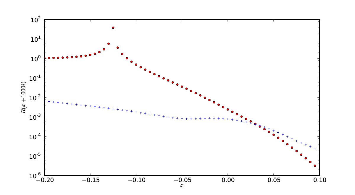
It has been observed that the convergence rate depends both on the parameters of the Schottky surface and also on the complex parameter $s$ [6, 18]. The convergence rate depends very strongly on $\operatorname{Re}(s)$ and very weekly on $\operatorname{Im}(s)$ . As in [6], we can use the relative error term,

R_{n}(s):=\frac{|Z_{X}^{(n-1)}(s)-Z_{X}^{(n)}(s)|}{Z_{X}^{(n)}(s)},

to compare convergence rates. Figure 7 shows a comparison of relative error terms for the surface $X_{3,0.1723}$ which corresponds to a 3-funneled Schottky surface with funnel-width $\ell=12$ . We compare the error term obtained by the symmetry factorized zeta function (5.13) of order 6 (blue crosses) with the non-reduced zeta function as used in [6, 18] of order 11 (red dots). Even though we use a much smaller order for the approximation of the symmetry factorized zeta function, the relative error term is significantly smaller for most $s$ values. Especially for $\operatorname{Re}(s)<0$ , the advantage of the symmetry factorized zeta function becomes very dramatic. If one requires a relative accuracy of $10^{-2}$ the non-reduced zeta function of order 11 allows the calculation of the zeta function only up to $\operatorname{Re}(s)\approx 0$ while the symmetry factorized zeta function of order 6 already allows a calculation up to $\operatorname{Re}(s)\approx-0.2$ . The benefit of the symmetry reduction becomes even clearer if one considers how many periodic orbits $u_{\mathbf{w}}$ have to be calculated in the two cases. For the non-reduced zeta function of order 11 one needs more then 170000 periodic orbits (c.f. [6, Table 1]) the symmetry-reduced zeta function of order 6, however, requires only the calculation of 41 periodic orbits.

This gain of efficiency can be used to calculate resonances in much larger domains. For example, Figure 8 shows the resonance spectrum for the surface $X_{3,0.1723}$ . Without symmetry reduction the numerical accessible resonance range was restricted [6] to $\operatorname{Re}(s)\gtrsim 0$ . The symmetry reduction allows us to calculate the resonances easily up to $\operatorname{Re}(s)=-0.3$ , increasing the width of the resonance strip by a factor of $4$ .

Another significant benefit of the symmetry factorization is that it provides additional information on the resonance spectrum. The factorization (5.9) allows us to associate the zeros of the Selberg zeta function to specific unitary irreducible representations of the symmetry group. As discussed above, the symmetry group of the symmetric 3-funneled surface is given by $D_{3}\times\mathbb{Z}_{2}$ . Via its action on the symbols, this group can be realized as a permutation group on 6 elements. One then calculates that the group has 6 conjugacy classes and thus 6 irreducible representations. The character table is given in Table 1. As Figure 8 illustrates, the resonance-chain structure corresponds with the symmetry reductions. However, one chain does not correspond to one only representation, as we might have expected, but rather to a pair of representations. The resonances on each chain alternate between the two corresponding representations. Intuitively this alternating behavior can be understood as follows: According to Definition 5.1 all the symmetric $n$ -funneled Schottky surfaces consist of two copies of $\tilde{\mathcal{S}}\subset\mathbb{D}$ that are glued together along the geodesic boundary, so the surfaces are symmetric with respect to the reflections along the plane in which the two copies are glued together and each resonant state is either symmetric or antisymmetric with respect to this reflection. Those states which are antisymmetric must vanish at the boundaries of $\tilde{\mathcal{S}}$ and can thus be considered as resonant states of the open hyperbolic billiard $\tilde{\mathcal{S}}$ with Dirichlet boundary conditions. Those states that are symmetric can be seen as resonant states of the hyperbolic billiard with Neumann boundary conditions. Looking at the character table (Table 1), we see that the two representations on each chain differ exactly by their symmetry with respect to the reflection on the gluing plane which is represented by the permutation $(1,4)(2,5)(3,6)$ . Each chain thus corresponds to one specific symmetry type of the hyperbolic billard $\tilde{\mathcal{S}}$ and the alternating behavior comes from switching between Dirichlet and von-Neumann boundary conditions. The same phenomenom is observed in the case of the symmetric 4-funneled surface (Figure 10) as well as for the non-symmetric 3-funneled surface (Figure 11). Note that this observation also fits the findings in [2, 34], where it has been shown that the chain structure is determined by the ratio of the periodic orbit lengths. For the Schottky surfaces considered here this ratio is already fully determined by the geometry of the hyperbolic billiards $\tilde{\mathcal{S}}$ , so we also expect the chain structure to be determined by one copy of $\tilde{\mathcal{S}}$ . The fact of gluing two copies of $\tilde{\mathcal{S}}$ together only doubles the length of all closed geodesics and and thus doubles the number of resonances on the chains by allowing them to alternate between symmetric and antisymmetric types.

	()	(2,3)(5,6)	(1,2,3)(4,5,6)	(1,4)(2,5)(3,6)	(1,4)(2,6)(3,5)	(1,5,3,4,2,6)
$I_{1}$	1	1	1	1	1	1
$I_{2}$	1	1	1	-1	-1	-1
$II_{1}$	1	-1	1	1	-1	1
$II_{2}$	1	-1	1	-1	1	-1
$III_{1}$	2	0	-1	-2	0	1
$III_{2}$	2	0	-1	2	0	-1

Table 1: Character table of the symmetry group

D_{3}\times\mathbb{Z}_{2}

of the symmetric 3-funneled surfaces

X_{3,\psi}

. In the first line the representatives of the conjugacy classes are given in cycle notation, where

D_{3}\times\mathbb{Z}_{2}

is realized as a permutation group on the symbols of the flow-adapted IFS. The following six lines represent the characters of the six unitary irreducible representations of this group.

	()	(2,4)(6,8)	(1,2)(3,4) (5,6)(7,8)	(1,2,3,4) (5,6,7,8)	(1,3)(2,4) (5,7)(6,8)	(1,5)(2,6) (3,7)(4,8)	(1,5)(2,8) (3,7)(4,6)	(1,6)(2,5) (3,8)(4,7)	(1,6,3,8) (2,7,4,5)	(1,7)(2,8) (3,5)(4,6)
$I_{1}$	1	1	1	1	1	1	1	1	1	1
$I_{2}$	1	1	1	1	1	-1	-1	-1	-1	-1
$II_{1}$	1	1	-1	-1	1	1	1	-1	-1	1
$II_{2}$	1	1	-1	-1	1	-1	-1	1	1	-1
$III_{1}$	1	-1	-1	1	1	-1	1	1	-1	-1
$III_{2}$	1	-1	-1	1	1	1	-1	-1	1	1
$IV_{1}$	1	-1	1	-1	1	-1	1	-1	1	-1
$IV_{2}$	1	-1	1	-1	1	1	-1	1	-1	1
$V_{1}$	2	0	0	0	-2	2	0	0	0	-2
$V_{2}$	2	0	0	0	-2	-2	0	0	0	2

Table 2: Character table of the symmetry group

D_{4}\times\mathbb{Z}_{2}

of the symmetric 4-funneled surfaces

X_{4,\psi}

. In the first line the representatives of the conjugacy classes are given in cycle notation, where

D_{4}\times\mathbb{Z}_{2}

is realized as a permutation group on the symbols of the flow-adapted IFS. The following six lines represent the characters of the ten unitary irreducible representations of this group.

Finally, the symmetry decomposition enables us to study the resonance structure of surfaces which were previously not treatable numerically. As an example, we show the resonance structure of the 3-funneled surface $X_{3,0.5930}$ (Figure 9) which corresponds to a funnel-width of 7 and the 4-funneled surface $X_{4,0.1010}$ (Figure 10) which corresponds to a funnel-width of 13. For the 3-funneled surface one observes again resonance chains on a large $\operatorname{Im}(s)$ range, where each chain is composed of resonances belonging to two representations. As expected from the observations in [2], these chains have a much stronger curvature in comparison to the resonance chains for the surface $X_{3,0.1723}$ . For the 4-funneled surface there are no resonance chains visible on a comparable scale to the 3-funneled surfaces. Only if one zooms in strongly on the $\operatorname{Im}(s)$ -scale and colors the resonances according to the different representations can one see strongly curved chains that are again each composed of contributions from two different representations. This different behavior between symmetric 3- and 4-funneled surfaces has been predicted in [2], because 4-funneled surface do not have naturally a strong clustering behavior in their primitive length spectrum. A surprising feature, however, is that there is one very stable resonance chain along the imaginary axis related to the two 2-dimensional representations $V_{1}$ and $V_{2}$ .

As we noted in Example 3.2, in the case $X_{l_{1},l_{1},l_{3}}$ with $l_{1}\neq l_{3}$ , the symmetry group is $\mathbb{Z}_{2}\times\mathbb{Z}_{2}$ , which has four one-dimensional irreducible representations, with the character table shown in Table 3. Proposition 5.7 also applies in this case, and the improvement in convergence properties for the reduced zeta function is impressive, even with this much smaller symmetry group. The error term with $n=6$ in this case is actually comparable to the corresponding error term for the full $D_{3}\times\mathbb{Z}_{2}$ reduction shown in Figure 7. In the $\mathbb{Z}_{2}\times\mathbb{Z}_{2}$ case, to calculate the symmetry-reduced zeta function up to $n=6$ requires a calculation of 196 periodic orbits, as opposed to 41 for the larger symmetry group. The gain in efficiency over the unreduced case is still very significant.

Figure 11 shows a companion plot to Figure 9, where the symmetry is broken by perturbing $l_{3}$ from $7$ to $7.01$ .

	()	(1,2)(3,4)	(1,3)(2,4)	(1,4)(2,3)
A	1	1	1	1
B	1	1	-1	-1
C	1	-1	1	1
D	1	-1	-1	1

Table 3: Character table of the symmetry group

\mathbb{Z}_{2}\times\mathbb{Z}_{2}

of the surface

X_{7,7,7.01}

5.3 Numerical investigations of the spectral gap

As illustrated in the previous subsection the symmetry factorization of the zeta function allows the numerical calculation of the resonance structure on Schottky surfaces that were previously not accessible. In this subsection we will use these convergence improvements in order to investigate the parametric dependence of the spectral gap numerically.

Let us first recall the notion of a spectral gap: By the work of Patterson [25, 26], it is known that the resonance with the largest real part is always located at the critical exponent $\delta$ and that all other resonances $s\in\textup{Res}(X)\setminus\{\delta\}$ satisfy $\operatorname{Re}(s)<\delta$ . By a spectral gap we denote a positive number $\varepsilon>0$ such that for

G_{0}(X):=\sup\{\operatorname{Re}(s),\penalty\ s\in\textup{Res}(X)\setminus\{\delta\}\}

one has $G_{0}(X)<\delta-\varepsilon$ . From the positivity and self-adjointness of $\Delta_{X}$ it follows that all resonances with $\operatorname{Re}(s)>1/2$ lie in the interval $(\tfrac{1}{2},1)$ . Consequently, if $\delta>\tfrac{1}{2}$ the existence of such a gap is immediate. For $\delta\leq\tfrac{1}{2}$ the existence of such a gap has been shown by Naud [22].

A related notion is the asymptotic spectral gap. If we introduce for $K\geq 0$ ,

G_{K}(X):=\sup\{\operatorname{Re}(s):\penalty\ s\in\textup{Res}(X)\setminus\{\delta\}\textup{ and }|\operatorname{Im}(s)|\geq K\},

then the asymptotic spectral gap can be defined by

G_{\infty}(X):=\lim_{K\to\infty}G_{K}(X).

While up to now there is not any explicit upper bound known (see [17] for a lower bound), Jakobsen and Naud made the conjecture [17], that for convex co-compact groups one has

G_{\infty}(X)=\frac{\delta}{2}.

In [6] the dependence of the asymptotic spectral gap on $\delta$ was examined. However, the numerically accessible resonance data could not support the above conjecture because of the limitation to small values of $\delta$ . Using the symmetry reduction we want to extend the $\operatorname{Im}(s)$ range in which the resonances for a given surface can be calculated as well as the range of critical exponents $\delta$ , i.e. the range of surfaces for which resonances can be calculated. This will provide a more thorough study of the spectral gap as well as the asymptotic spectral gap.

Let $X_{n_{f},\psi}$ be a symmetric $n$ -funneled surface. According to (5.9) the Selberg zeta function factorizes into its symmetry reduced zeta functions $Z_{X_{n_{f},\psi}}^{\chi}(s)$ . Beyond the convergence improvement, this symmetry factorization also allows to study the question of spectral gap and asymptotic spectral gap for particular irreducible representations $\chi$ . We define,

G^{\chi}_{K}(X_{n_{f},\psi}):=\sup\{\operatorname{Re}(s):\penalty\ s\in\mathbb{C}\setminus\{\delta\},\penalty\ Z_{X_{n_{f},\psi}}^{\chi}(s)=0,\penalty\ |\operatorname{Im}(s)|>K\}

In Figure 12 we compare the dependence of the spectral gap for the different representations for the surface $X_{3,0.3631}$ (which corresponds to a surface where the shortest geodesics have lengths equal to 9). To be more precise, Figure 12 shows the resonance envelope functions,

h^{\chi}_{w}(t):=\max\{\operatorname{Re}(s):\penalty\ Z_{X_{n_{f},\psi}}^{\chi}(s)=0,\penalty\ |\operatorname{Im}(s)-t|\leq w\}.

As expected from the observation of the resonance chain structures (see Figure 8 and 9) the envelope functions of the representations $I_{1}$ and $I_{2}$ are equal to such a good approximation that no difference can be seen in the plot. This also holds for the pairs $II_{1}$ and $II_{2}$ as well as $III_{1}$ and $III_{2}$ . Additionally one observes that, while the envelope functions of the representations $I$ and $II$ locally differ slightly from each other, the spectral gaps

G^{\chi}_{K}(X_{n_{f},\psi})=\sup\limits_{t>K+w}h^{\chi}_{w}(t)

of all the one-dimensional representations are equal to each other up to a very good precision and additionally they are all equal to the spectral gap of the non-reduced system. Only the two-dimensional representations seem to lead to different spectral gaps. The same observation has been made for all other surfaces that we have examined. We therefore conjecture, that for the determination of the asymptotic spectral gap it is enough to study the asymptotic spectral gap of the trivial representation.

Besides the numerical observations, this conjecture is supported by the following heuristic arguments. Morally, the symmetry reduced zeta function associated to the trivial representation corresponds to the Selberg zeta function of a hyperbolic billiard of the symmetry reduced fundamental domain with Neumann boundary conditions. The question of explicit bounds on the asymptotic spectral gap on convex co-compact surfaces can also be interpreted in a more general context of open quantum systems with a fractal trapped set as an improvement of the known topological pressure bounds (c.f. [24, Section 8.2]). If such a general improvement of these spectral gap bounds exists, then it should of course be also visible for all symmetry reduced zeta functions that can be interpreted as hyperbolic billiards with certain boundary conditions. Thus, in particular, it should hold also for the symmetry reduction with respect to the trivial representation. For this reason, we will from now on focus on the symmetry reduced spectral gap of the trivial representation $G^{I_{1}}_{K}(X_{n_{f},\psi})$ in more detail.

Both plots in Figure 13 show the envelope function of the surface $X_{3,0.3631}$ for the trivial representation but on different scales. In the upper plot one sees, that the envelope function $h_{100}(t)$ shows a beating structure. The oscillations correspond to those that have been observed in [6, Figure 22], however one observes that there is a revival of the amplitudes at about $t=25000$ , where the envelope function nearly reaches $\delta$ again. On the lower plot in figure 13 we see the envelope function $h_{w}(t)$ but now for a different window width $w=2500$ and on a $t$ -range which is two orders of magnitude larger. The envelope function again oscillates and the amplitudes show again a nearly periodic modulation. However, now one oscillation of the envelope function in the lower plot corresponds to the modulation of the amplitudes in the upper plot. The beating structure thus repeats at different scales. A convergence of the asymptotic spectral gap towards the conjecture of $\delta/2$ can not be observed. However, the value of $\delta/2$ seems to have an importance as it is on both scales the turning point from where the amplitude oscillations start to grow again. Figure 14 shows that these oscillating envelope functions are also not only an artifact of the 3-funneled Schottky surfaces, that show a particular strong clustering in the length spectrum (cf. [34]), but that they also occur for 4-funneled surfaces.

These oscillations of the envelope function make it difficult to extract reliable information on the asymptotic spectral gap from numerical data. Even if the envelope function has decreased to a certain value within the numerically accessible range, one cannot rule out large-scale oscillations that would return it to higher values.

We nevertheless want to examine the parametric dependence of the asymptotic spectral gap numerically. In particular, we wish to examine the dependence of $G_{K}(X)$ on the critical exponent $\delta$ for 3- and 4-funneled surfaces. In order to avoid effects that come from the finite range of numerically accessible resonances we make sure that $K\ll\max_{\operatorname{Im}}$ , where $\max_{\operatorname{Im}}$ is the maximum of imaginary parts of the accessible resonances. Figure 15 shows $G^{I_{1}}_{0}(X)$ and $G^{I_{1}}_{100}(X)$ for different 3- and 4-funneled surfaces in dependence of the critical exponent $\delta$ . As expected from the oscillation of the envelope function, the values of $G^{I_{1}}_{0}(X)$ and $G^{I_{1}}_{100}(X)$ are very similar for all surfaces. We also checked, that this doesn’t change if one goes to higher values of $K$ provided that $K\ll\max_{\operatorname{Im}}$ is fulfilled. For strongly open surfaces with $\delta\lesssim 0.3$ there is no visible macroscopic gap between the leading resonance at $\delta$ and the bulk of the resonances. This, however, changes as one goes to more closed surfaces with $\delta\approx 0.5$ . Here one sees a clear gap, and there even seems to be a universal behavior of this gap, as the values for the 3- and 4-funneled surfaces lie on approximately the same line. Note that a very similar behavior of the spectral gap has been observed in numerical and experimental data of quantum resonances in $n$ -disk systems [1].

The examples which we have presented in this subsection demonstrate that the symmetry reduction allows a much more detailed study of the spectral gaps. The efficiency gain that results from restricting our attention to the trivial representation allows us to study the behavior for the envelope function for higher imaginary parts and additionally to study the spectral gap on weakly open surfaces with $\delta\approx 0.5$ . Concerning the higher imaginary parts, we could not observe that this improves the spectral gap significantly. We have rather observed that the oscillating behavior of the envelope function repeats itself on different scales. On all surfaces which we could handle numerically the asymptotic spectral gap was already determined quite well by the resonances with low imaginary parts. The study of the weakly open surfaces with $\delta\approx 0.5$ showed however an interesting macroscopic spectral gap which not only holds asymptotically but already from the second resonance on. Especially the fact that the 3-funneled and 4-funneled surfaces behave equally, and that a similar behavior has also been observed for $n$ -disk systems [1], suggests that there is a universal principle behind this behavior. To our knowledge there are neither any rigorous nor any heuristic formulas known that describe these observations, and we consider the determination of such formulas as an important task.

Appendix A Numerical implementation of symmetry-reduced zeta functions for n-funneled Schottky surfaces

In this section we will discuss some practical aspects of the numerical implementation of the symmetry-reduced Selberg zeta functions for symmetric $n$ -funneled Schottky surfaces. For a given surface $X_{n_{f},\psi}$ , a given character $\chi$ , and a point $s\in\mathbb{C}$ , the task is to calculate the truncated Selberg zeta function (5.14) at a finite order $n$ . This task basically splits into two subtasks: First one has to calculate $T^{\chi}_{[{\mathbf{w}}],l}(s)$ for every pair $([{\mathbf{w}}],l)\in\left[\mathcal{W}^{G}\right]\times\mathbb{N}$ that appears in the sum. Then one has to handle the combinatorial task of combining these $T^{\chi}_{[{\mathbf{w}}],l}$ to the products and sums according to (5.14).

By (5.12) the first task reduces, for a given $({\mathbf{w}},l)$ , to the calculation of $\phi^{\prime}_{w^{m_{\mathbf{w}}}}(u_{{\mathbf{w}}})$ . By the proof of Proposition 5.5 this quantity is directly related to the displacement length of the hyperbolic transformation $T(w^{m_{\mathbf{w}}})$ , which was defined for a closed word in (5.2). Using the formula,

\cosh(l(T)/2)=\frac{1}{2}\left|\operatorname{Tr}(T)\right|,

relating the displacement length $l(T)$ to the trace of the hyperbolic element $T\in SL(2,\mathbb{R})$ , we obtain

\phi^{\prime}_{w^{m_{\mathbf{w}}}}(u_{{\mathbf{w}}})=\exp\left(-2l(T(w^{m_{\mathbf{w}}}))\right)=\exp\left(-2\cosh^{-1}\left(\frac{|\textup{Tr}(T(w^{m_{\mathbf{w}}}))|}{2}\right)\right).

The second task can be significantly simplified by using the recurrence relation proposed in [12, Section 7]. We can write (5.14) in the form

Z^{\chi,(n)}_{X_{n_{f},\psi}}(s)=1+\sum\limits_{N=1}^{n}\sum\limits_{r=1}^{N}B^{\chi}_{N,r}(s)

where

B^{\chi}_{N,r}(s):=\frac{1}{r!}\sum\limits_{t\in P(N,r)}\prod\limits_{k=1}^{r}a^{\chi}_{t_{k}}(s).

Here $P(N,r)$ is the set of all $r$ -partitions of $N$ , i.e. the set of all $r$ -tuples $t=(t_{1},\ldots,t_{r})\in\mathbb{N}_{>0}^{r}$ such that $t_{1}+\ldots+t_{r}=N$ and

a^{\chi}_{t_{k}}(s):=-\sum\limits_{\begin{array}[]{c}{\scriptstyle([{\mathbf{w}}],l)\in\left[\mathcal{W}^{G}\right]\times\mathbb{N}_{>0}}\\ {\scriptstyle n_{\mathbf{w}}\cdot l=t_{k}}\end{array}}T^{\chi}_{[{\mathbf{w}}],l}(s).

To implement this strategy it is sufficient to calculate $a^{\chi}_{t}(s)$ for all $t=1,\ldots,n$ . The coefficients $B^{\chi}_{N,r}(s)$ can then be obtained by the recurrence relation,

B^{\chi}_{N,r}(s)=\frac{1}{r}\sum\limits_{t=1}^{N-r+1}B^{\chi}_{N-t,r-1}(s)\cdot a^{\chi}_{t}(s),

with the start value $B^{\chi}_{N,1}(s)=a^{\chi}_{N}(s)$ .

In order to calculate the coefficients $a^{\chi}_{t}(s)$ one has to determine a representative for each class $[{\mathbf{w}}]\in\left[\mathcal{W}^{G}\right]$ for $0<n_{\mathbf{w}}\leq n$ . Note this task need only be performed once for all surfaces $X_{n_{f},\psi}$ with a fixed number of funnels $n_{f}$ , so efficiency is not of the utmost importance. (The numerically most expensive task consists in calculating the values of $Z^{\chi,(n)}_{X_{n_{f}}}(s)$ several million times in order to determine its zeros at a good precision.) Nevertheless, we want to briefly describe an elegant and fast way to determine all such representatives.

We define the symmetry-reduced symbolic dynamics for a $n_{f}$ -funneled surface to be the complete symbolic dynamics with the symbols

\left\{\frac{-n_{f}-1}{2},\ldots,-1,1,\ldots,\frac{n_{f}-1}{2}\right\}\textup{ if }n_{f}\textup{ uneven},

and

\left\{\frac{-n_{f}-2}{2},\ldots,-1,0,1,\ldots,\frac{n_{f}-2}{2}\right\}\textup{ if }n_{f}\textup{ even}.

The term “complete” means that all sequences of symbols are allowed, i.e. the adjacency matrix has the value 1 in each entry. We denote the set of words of the symmetry-reduced symbolic dynamics by $\mathcal{W}_{sr}$ . The idea of this symmetry-reduced coding has successfully been used in for 3- and 4-disk systems [10] as well as for 5-disk systems [1].

The symmetry-reduced coding can be understood in the example of the 3-funneled surface as follows: A closed geodesic can be represented on two copies of $\tilde{S}\subset\mathbb{D}$ . Because the two copies are glued together along the circles $c_{i}$ , the geodesic alternates between these two copies. If it hits one circle $c_{i}$ it leaves again at the corresponding partner $c_{i+3}$ or $c_{i-3}$ , respectively. Since there is no geodesic in $\tilde{S}$ entering and leaving the same boundary circle $c_{i}$ , the geodesic has either to leave the region $\tilde{S}$ by the next circle in clockwise direction or by the next circle in counterclockwise direction. Given a word $w_{sr}\in\mathcal{W}_{sr}$ , which consists of a sequence of the symbols $\{1,-1\}$ , we can construct the corresponding representative in $\mathcal{W}^{G}$ as follows. Start at an arbitrary circle $c_{\textup{start}}$ , with an arbitrary orientation. At each step we proceed to the next circle in the current orientation, but then we either preserve or reverse the orientation for the next step, according to sign of the current symbol. After passing through all symbols of the word $w_{sr}$ , one ends at a circle $c_{\textup{end}}$ with a final orientation. Now there is a unique symmetry of the surface that maps $c_{\textup{end}}$ to $c_{\textup{start}}$ and the final orientation to the initial orientation. We define $g$ to be the associated group element in $D_{3}\times\mathbb{Z}_{2}$ . Furthermore, by collecting the indices of the circles from which the geodesic entered the domain $\mathcal{S}$ , we get a word $w=(w_{0},w_{1},\ldots,w_{n})\in\mathcal{W}$ . The representative associated to $w_{sr}$ is then exactly the pair ${\mathbf{w}}=(w,g)$ .

For an uneven number of funnels $n_{f}>3$ , we must allow for the possibility to leave $\tilde{S}$ through the next $2,3,\ldots,(n_{f}-1)/2$ circles in either the clockwise or counterclockwise direction. The symbols $n=1,\ldots,(n_{f}-1)/2$ thus correspond to “go $n$ steps in the current orientation and keep the orientation”, and the symbols $-n=-1,\ldots,-(n_{f}-1)/2$ correspond to “go $n$ steps in the current orientation and switch the orientation for the next step”. In the even case, one has to include also the possibility of stepping forward $n_{f}/2$ circles. Here it makes no difference which orientation is taken. This possibility is encoded by the label $0$ and the current orientation for the further steps is not changed in this case.

Via this algorithm, one can identify words in the reduced symbolic dynamics with elements ${\mathbf{w}}\in\mathcal{W}^{G}$ . Note that the idea of the reduced symbolic dynamic is not to encode the absolute position of the closed geodesics, but rather to encode the relative changes as one moves along the geodesic. The reduced symbolic dynamic is thus by construction compatible with the action of the symmetry group in the following sense. If ${\mathbf{w}}$ and ${\mathbf{w}}^{\prime}$ are two elements in $\mathcal{W}^{G}$ obtained from the same reduced word $w_{sr}$ using a different starting circle or orientation, then they are in the same $G$ -orbit in $\mathcal{W}^{G}$ and vice versa. It is easy to check that the shift action on $\mathcal{W}_{sr}$ corresponds to the shift action on $\mathcal{W}^{G}$ and similarly for the composition of words. Thus one has identified the orbits of prime words under the shift action in $\mathcal{W}$ with the prime elements in $\left[\mathcal{W}^{G}\right]$ , which provides an easy means to generate a list of representatives of the elements in $\left[\mathcal{W}^{G}_{\mathrm{prime}}\right]$ .

Let us return to the 3-funneled surface for an illustrating example. The alphabet consists of two symbols $+1$ and $-1$ and accordingly there are only the two words $(1)$ and $(-1)$ of length one. Let us write $\{c_{i},\pm\}$ for a visit of the circle $c_{i}$ with positive/negative orientation. Starting with $c_{1}$ with positive orientation, the word $(1)$ leads to the sequence $\{c_{1},+\},\{c_{5},+\}$ while the word $(-1)$ leads to $\{c_{1},+\},\{c_{5},-\}$ . Now the symmetry group of the 3-funneled surface $D_{3}\times\mathbb{Z}_{2}$ , represented as a permutation group of the six symbols, contains two elements that map $c_{5}$ to $c_{1}$ , namely $(1,6,2,4,3,5)$ and $(1,5)(2,4)(3,6)$ . While the first one preserves the orientation of the labels, the second one changes them (see Figure 16).

The symmetry reduced word $(1)$ thus corresponds to the pair ${\mathbf{w}}_{(1)}=((1,5),(1,6,2,4,3,5))\in\mathcal{W}^{G}$ while the symmetry reduced word $(-1)$ corresponds to ${\mathbf{w}}_{(-1)}=((1,5),(1,5)(2,4)(3,6))\in\mathcal{W}^{G}$ . While the multiplicity of the first word is $m_{{\mathbf{w}}_{(1)}}=6$ for the second word we have $m_{{\mathbf{w}}_{(-1)}}=2$ . The closed word ${\mathbf{w}}_{(-1)}^{m_{{\mathbf{w}}_{(-1)}}}$ then corresponds to a geodesic that winds one time around one of the funnels while the closed word ${\mathbf{w}}_{(1)}^{m_{{\mathbf{w}}_{(1)}}}$ weaves around all three funnels (see Figure 17 for a sketch of the two geodesics).

The symmetry-reduced words of length two are given by $(1,1),(-1,-1)$ , $(1,-1)$ and $(-1,1)$ . The first two elements are not prime, and last two are related to each other by the shift action. At length two it thus suffices to study the single symmetry reduced word $(1,-1)$ . Applying the algorithm yields a sequence $(\{c_{1},+\},\{c_{5},+\},\{c_{3},-\})$ . The corresponding closing group element is given by $(1,3)(4,6)$ and the geodesic of the closed word ${\mathbf{w}}_{(1,-1)}^{m_{{\mathbf{w}}_{(1,-1)}}}$ winds in a figure-eight shape around two funnels (see Figure 17).

Appendix B Convergence rate estimates

For a general holomorphic IFS we have noted that the dynamical zeta function $d_{V}(z)$ is an entire function of $z$ and therefore the corresponding power series

d_{V}(z)=1+\sum_{n=1}^{\infty}d_{n}z^{n},

converges absolutely for all $z$ . In the application to Selberg zeta functions, we would like to understand the rate of convergence of this series when $z=1$ .

To estimate the coefficients (following ideas from [18]), we first note that the Fredholm definition of the determinant $d_{V}(z):=\det(1-z\mathcal{L}_{V})$ allows us to write

d_{n}=(-1)^{n}\operatorname{Tr}(\wedge^{n}\mathcal{L}_{V}),

where $\wedge^{n}A$ denotes the $n$ -th antisymmetric tensor power of the operator $A$ . We can bound the $d_{n}$ by the trace norm of $\wedge^{n}\mathcal{L}_{V}$ , which can be expressed in terms of the singular values of $\mathcal{L}_{V}$ . Using the Hadamard bound on $n\times n$ matrices with entries smaller than or equal to one, this yields the estimate,

\left|d_{n}\right|\leq n^{n/2}\sum_{i_{1}<\dots<i_{n}}\mu_{i_{1}}(\mathcal{L}_{V})\dots\mu_{i_{n}}(\mathcal{L}_{V}).

(B.1)

To estimate the singular values of $\mathcal{L}_{V}$ is relatively straightforward. Let us introduce an explicit orthonormal basis $\{\psi_{n}\}$ for $\mathcal{B}(D_{j})$ ,

\psi_{n}(z):=\sqrt{\frac{n+1}{\pi r_{j}^{2}}}\left(\frac{z-m_{j}}{r_{j}}\right)^{n},

where $m_{j}$ and $r_{j}$ denote the center and radius of $D_{j}$ , respectively. According to (2.3), for each $i\rightsquigarrow j$ the transfer operator $\mathcal{L}_{V}$ has a component

L_{i,j}:\mathcal{B}(D_{j})\to\mathcal{B}(D_{i}),

given by

L_{i,j}f(u)=V(\phi_{i,j}(u))f(\phi_{i,j}(u)),

for $u\in D_{i}$ , $f\in\mathcal{B}(D_{j})$ . If $\eta_{ij}$ is defined by

\eta_{ij}:=d(\phi_{i,j}(D_{i}),\partial D_{j})>0,

then the action of the transfer operator on a basis element can be estimated explicitly by

\left\|L_{i,j}\psi_{n}\right\|_{\mathcal{B}(D_{i})}\leq\sqrt{n+1}\>\frac{r_{i}}{r_{j}}\left(1-\frac{\eta_{ij}}{r_{j}}\right)^{n}\sup_{u\in D_{i}}\left|V(\phi_{i,j}(u))\right|.

(B.2)

Note that these bounds decay exponentially as a function of $n$ , at a rate determined only by $\eta_{ij}$ and $r_{j}$ .

By min-max, we can combine these basis element estimates into a singular value estimate,

\mu_{k}(L_{i,j})\leq\sum_{n=k}^{\infty}\left\|L_{i,j}(s)\psi_{n}\right\|_{\mathcal{B}(D_{i})}.

(B.3)

These component estimates can then be combined into an estimate of the singular values of the full transfer operator. The result is an estimate

\mu_{k}(\mathcal{L}_{V})\leq CM_{V}e^{-cn},

where $c>0$ and $C$ depend only on the geometric structure of the IFS, and

M_{V}:=\sup_{i\rightsquigarrow j}\sup_{u\in D_{i}}\left|V(\phi_{i,j}(u))\right|.

Using this estimate in (B.1) then gives

\left|d_{n}\right|\leq C^{n}M_{V}^{n}n^{n/2}e^{-cn^{2}}.

Note that although the decay of the coefficients is always super-exponential, the convergence rate could still be extremely poor for small $n$ if $V$ is large.

For the symmetry-reduced transfer operator $\mathcal{L}_{V}^{\chi}:=\mathcal{L}_{V}P_{\chi}$ , the same estimate applies, because

\mu_{k}(\mathcal{L}_{V}^{\chi})\leq\left\|P_{\chi}\right\|\mu_{k}(\mathcal{L}_{V}).

(On $\mathcal{B}(D)$ the $P_{\chi}$ are not orthogonal projections, but of course they are still bounded operators.) In cases where the disks are of roughly equal sizes we’d expect $\left\|P_{\chi}\right\|\approx 1$ , so this estimate does not explain the observation in Section 5.2 that convergence rates seem to be much higher in the symmetry-reduced case.

We can interpret this improved convergence as a result of dramatically reducing the size of the Hilbert spaces on which the transfer operator acts. Let us suppose, for example, that the singular value bounds for each component of the transfer operator given in (B.2) and (B.3) give uniform bounds

\mu_{k}(L_{i,j})\leq CM_{V}e^{-\alpha n}.

(B.4)

For a Schottky group with 2 generators, we need to combine singular estimates for 12 components $L_{i,j}$ to estimate the singular values of $\mathcal{L}_{V}$ itself. The additive Fan inequality (see e.g. [4, Theorem A.18]) allows us to combine these estimates for the 12 components into the estimate

\mu_{k}(\mathcal{L}_{V})\leq 12CM_{V}e^{-\alpha n/12}.

In other words, whatever decay rate we achieved for components in (B.4) might be considerably degraded for the full transfer operator.

On the other hand, for $\mathcal{L}_{V}^{\chi}$ we obtain a basis for all of $\mathcal{B}^{\chi}$ by applying $P^{\chi}$ to the basis $\psi_{n}$ for a single disk. If we assume that the disks are of roughly equal radii, so that $P^{\chi}$ is close to orthogonal, then we can replace the estimates (B.2) with an estimate that applies to a full basis $\{\psi_{n}\}$ for $\mathcal{B}^{\chi}$ , by taking the maximum over $i,j$ . Then instead of the component-wise estimate (B.4), we would have an estimate for the singular values of the full transfer operator,

\mu_{k}(\mathcal{L}_{V}^{\chi})\leq CM_{V}e^{-\alpha n},

with no loss of decay rate in the exponent $\alpha$ . Of course, this argument involves upper bounds which are not necessarily effective in either case. But it perhaps suggests a plausible mechanism for the dramatically improved decay rates in the symmetry-reduced numerical calculations.

Another heuristic justification for the good convergence of the symmetry-reduced zeta function is the “shadowing orbits” argument made by Cvitanovic and Eckhardt [9, 10] in the setting of $3$ -disk systems. They propose that in the Taylor coefficients $d_{n}$ with $n\geq 2$ , the contributions of long closed geodesics are largely canceled by the combination of shorter geodesics. Translated to the three-funneled surface and the case of the trivial representation $\chi=I_{1}$ , these arguments can be illustrated at the following example: According to Appendix A the pairs ${\mathbf{w}}_{(1)}=((1,5),(1,6,2,4,3,5))$ and ${\mathbf{w}}_{(-1)}=((1,5),(1,5)(2,4)(3,6))$ are the representatives of the only classes of primitive $G$ -closed words of length $1$ and ${\mathbf{w}}_{(1,-1)}=((1,5,3),(1,3)(4,6))$ is a representative of the only class of length $2$ . Using (5.14) we can write

d_{1}^{I_{1}}=-\left(T^{I_{1}}_{[{\mathbf{w}}_{(1)}],1}+T^{I_{1}}_{[{\mathbf{w}}_{(-1)}],1}\right)

(B.5)

and

d_{2}^{I_{1}}=\frac{1}{2!}\left(T^{I_{1}}_{[{\mathbf{w}}_{(1)}],1}+T^{I_{1}}_{[{\mathbf{w}}_{(-1)}],1}\right)^{2}-\left(T^{I_{1}}_{[{\mathbf{w}}_{(1,-1)}],1}+T^{I_{1}}_{[{\mathbf{w}}_{(1)}],2}+T^{I_{1}}_{[{\mathbf{w}}_{(-1)}],2}\right).

(B.6)

From the definition (5.12) of $T^{I_{1}}_{[{\mathbf{w}}_{(1)}],1}$ and the identification of closed words and closed geodesics in Proposition 5.5 we have

T^{I_{1}}_{{\mathbf{w}}_{(1)},k}=\frac{1}{k}\frac{\exp(-skl_{(1)}/m_{{\mathbf{w}}_{(1)}})}{1-\exp(-kl_{(1)}/m_{{\mathbf{w}}_{(1)}})},

where $l_{(1)}$ is the length of the closed geodesic corresponding to the symmetry reduced word $(1)$ (see upper left part of Figure 17). Analogous expressions can be obtained also for the other terms. The crucial observation is that, for three funneled Schottky surfaces with sufficiently large funnel widths, there exists a base length $\ell$ with

l_{(1)}/m_{{\mathbf{w}}_{(1)}}\approx l_{(-1)}/m_{{\mathbf{w}}_{(-1)}}\approx\mathcal{\ell}\textup{ and }l_{(1,-1)}/m_{{\mathbf{w}}_{(1,-1)}}\approx 2\ell

Indeed this approximation is well satisfied for the surfaces which we consider. For example for the surface $X_{3,0.5930}$ the base length is given by $\ell=3.5$ and we have

l_{(1)}/m_{{\mathbf{w}}_{(1)}}=3.530,\quad l_{(-1)}/m_{{\mathbf{w}}_{(-1)}}=3.5\quad\textup{and}\quad l_{(1,-1)}/m_{{\mathbf{w}}_{(1,-1)}}=7.032.

Using the approximation of the lengths as well as the approximation $1-\exp(-k\ell)\approx 1$ we observe that the terms in (B.6) cancel each other. More precisely, one observes that the different combinations of $G$ -closed words of length $1$ cancel with those of length 2. This approximate canceling can also be observed for the higher Taylor coefficients, leading to very quick convergence.

Note that for the dynamical zeta function obtained by the standard Bowen-Series maps such a cancellation can not be observed due to the asymmetric treatment of the geodesics (cf. discussion in Example 3.2). Even when the dynamical zeta function is analytic in $z$ and the Taylor coefficients thus decay super-exponentially, the convergence is much slower in this case due to the non-optimal ordering of the geodesics. For non-reduced flow-adapted IFS and three funneled Schottky surfaces, [34, Lemma 5.6.] implies that such a cancellation occurs for the coefficients of order strictly larger than 6. Without symmetry reduction the lower coefficients do however not cancel completely as the symbolic dynamic is not complete and the remaining terms have been identified to be responsible for the structure of the resonance chains.

References

[1] S. Barkhofen. Microwave Measurements on n-Disk Systems and Investigation of Branching in correlated Potentials and turbulent Flows. PhD thesis, Marburg, Philipps-Universität Marburg, Diss., 2013, 2013.
[2] S. Barkhofen, F. Faure, and T. Weich. Resonance chains in open systems, generalized zeta functions and clustering of the length spectrum. Nonlinearity, 27:1829-1858, 2014.
[3] S. Barkhofen, T. Weich, A. Potzuweit, H-J. Stöckmann, U. Kuhl, and M. Zworski. Experimental observation of the spectral gap in microwave n-disk systems. Physical review letters, 110(16):164102, 2013.
[4] D. Borthwick. Spectral theory of infinite-area hyperbolic surfaces. Basel: Birkhäuser, 2007.
[5] D. Borthwick. Sharp geometric upper bounds on resonances for surfaces with hyperbolic ends. Analysis & PDE, 5(3):513–552, 2012.
[6] D. Borthwick. Distribution of resonances for hyperbolic surfaces. Experimental Mathematics, 23:25–45, 2014.
[7] J. Bourgain, A. Gamburd, and P. Sarnak. Generalization of Selberg’s $\frac{3}{16}$ theorem and affine sieve. Acta mathematica, 207(2):255–290, 2011.
[8] J. Button. All Fuchsian Schottky groups are classical Schottky groups. In The Epstein birthday schrift, pages 117–125. Geom. Topol. Publ., Coventry, 1998.
[9] P. Cvitanović and B. Eckhardt. Periodic-orbit quantization of chaotic systems. Physical review letters, 63(8):823–826, 1989.
[10] P. Cvitanovic and B. Eckhardt. Symmetry decomposition of chaotic dynamics. Nonlinearity, 6(2):277, 1993.
[11] L. Guillopé. Fonctions zêta de selberg et surfaces de géométrie finie. Adv. Stud. Pure Math, 21:33–70, 1992.
[12] L. Guillopé, K.K. Lin, and M. Zworski. The Selberg zeta function for convex co-compact Schottky groups. Communications in mathematical physics, 245(1):149–176, 2004.
[13] L. Guillopé and M. Zworski. Upper bounds on the number of resonances for non-compact Riemann surfaces. J. Funct. Anal., 129(2):364–389, 1995.
[14] L. Guillopé and M. Zworski. Scattering asymptotics for Riemann surfaces. Annals of mathematics, 145(3):597–660, 1997.
[15] L. Guillopé and M. Zworski. The wave trace for Riemann surfaces. Geometric & Functional Analysis GAFA, 9(6):1156–1168, 1999.
[16] D. Jakobson and F. Naud. On the resonances of convex co-compact subgroups of arithmetic groups. arXiv preprint arXiv:1011.6264, 2010.
[17] D. Jakobson and F. Naud. On the critical line of convex co-compact hyperbolic surfaces. Geometric and Functional Analysis, 22(2):352–368, 2012.
[18] O. Jenkinson and M. Pollicott. Calculating Hausdorff dimension of Julia sets and Kleinian limit sets. American Journal of Mathematics, 124(3):495–545, 2002.
[19] E. Jones, T. Oliphant, P. Peterson, et al. SciPy: Open source scientific tools for Python, 2001–.
[20] W. Lu, S. Sridhar, and M. Zworski. Fractal Weyl laws for chaotic open systems. Physical review letters, 91(15):154101, 2003.
[21] R.R. Mazzeo and R.B. Melrose. Meromorphic extension of the resolvent on complete spaces with asymptotically constant negative curvature. Journal of Functional analysis, 75(2):260–310, 1987.
[22] F. Naud. Expanding maps on Cantor sets and analytic continuation of zeta functions. Ann. Sci. Éc. Norm. Supér. (4), 38(1):116–153, 2005.
[23] F. Naud. Density and location of resonances for convex co-compact hyperbolic surfaces. Inventiones mathematicae, (3):723–750, 2014.
[24] S. Nonnenmacher. Spectral problems in open quantum chaos. Nonlinearity, 24(12):R123, 2011.
[25] S.J. Patterson. The limit set of a Fuchsian group. Acta mathematica, 136(1):241–273, 1976.
[26] S.J. Patterson. On a lattice-point problem in hyperbolic space and related questions in spectral theory. Arkiv för Matematik, 26(1):167–172, 1988.
[27] S.J. Patterson and P.A. Perry. The divisor of Selberg’s zeta function for Kleinian groups. Appendix A by Charles Epstein. Duke Math. J., 106(2):321–390, 2001.
[28] P. Perry. A poisson summation formula and lower bounds for resonances in hyperbolic manifolds. International Mathematics Research Notices, 2003(34):1837–1851, 2003.
[29] A. Potzuweit, T. Weich, S. Barkhofen, U. Kuhl, H.-J. Stöckmann, and M. Zworski. Weyl asymptotics: From closed to open systems. Physical Review E, 86(6):066205, 2012.
[30] D. Ruelle. Zeta-functions for expanding maps and Anosov flows. Inventiones mathematicae, 34(3):231–242, 1976.
[31] M. Schönert et al. GAP – Groups, Algorithms, and Programming – version 3 release 4 patchlevel 4. Rheinisch Westfälische Technische Hochschule, 1997.
[32] H. Schomerus and J. Tworzydło. Quantum-to-classical crossover of quasibound states in open quantum systems. Physical review letters, 93(15):154102, 2004.
[33] W. A. Stein et al. Sage Mathematics Software (Version 6.1.1). The Sage Development Team, 2014. http://www.sagemath.org.
[34] T. Weich. Resonance chains and geometric limits on schottky surfaces. arxiv:1403.7419 (to appear in Communications in mathematical physics).
[35] T. Weich, S. Barkhofen, U. Kuhl, C. Poli, and H. Schomerus. Formation and interaction of resonance chains in the open 3-disk system. New Journal of Physics, 16:033029, 2014.
[36] M. Zworski. Dimension of the limit set and the density of resonances for convex co-compact hyperbolic surfaces. Inventiones mathematicae, 136(2):353–409, 1999.

Symmetry reduction of holomorphic iterated function schemes and factorization of Selberg zeta functions

Abstract

1 Introduction

Theorem 1.1 ([27] Patterson-Perry 2001).

2 Holomorphic iterated function schemes and their transfer operators

Definition 2.1.

Remark 2.2.

Example 2.3.

Definition 2.4.

Remark 2.5.

Lemma 2.6.

Proof.

Definition 2.7 (transfer operator).

Example 2.8.

3 Trace formula for the symmetry-reduced transfer operator

Definition 3.1.

Example 3.2.

Proposition 3.3.

Proof.

4 Factorization of the zeta function

Theorem 4.1.

Proof.

Definition 4.2.

Lemma 4.3.

Proof.

Proposition 4.4.

Proof.

Lemma 4.5.

Proof.

Theorem 4.6.

Lemma 4.7.

Proof.

Corollary 4.8.

5 Application to Selberg zeta functions

5.1 Factorization of Selberg zeta functions for symmetric nn-funneled Schottky surfaces

Definition 5.1.

Lemma 5.2.

Proof.

Definition 5.3.

Proposition 5.4.

Proof.

Proposition 5.5.

Proof.

Lemma 5.6.

Proof.

5.2 Numerical calculations of resonances on Xnf,ψX_{n_{f},\psi}

Proposition 5.7.

Remark 5.8.

Proof.

5.3 Numerical investigations of the spectral gap

Appendix A Numerical implementation of symmetry-reduced zeta functions for n-funneled Schottky surfaces

Appendix B Convergence rate estimates

References

5.1 Factorization of Selberg zeta functions for symmetric $n$ -funneled Schottky surfaces

5.2 Numerical calculations of resonances on $X_{n_{f},\psi}$