The Offset Filtration of Convex Objects Thanks: Work by D.H. and D.S. has been supported in part by the Israel Science Foundation (grant no. 1102/11), by the German-Israeli Foundation (grant no. 1150-82.6/2011), and by the Hermann Minkowski–Minerva Center for Geometry at Tel Aviv University. M.K. acknowledges support by the Max Planck Center of Visual Computing and Communication.
Abstract
We consider offsets of a union of convex objects. We aim for a filtration, a sequence of nested cell complexes, that captures the topological evolution of the offsets for increasing radii. We describe methods to compute a filtration based on the Voronoi partition with respect to the given convex objects. We prove that, in two and three dimensions, the size of the filtration is proportional to the size of the Voronoi diagram. Our algorithm runs in in the -dimensional case and in expected time , for any , in the -dimensional case. Our approach is inspired by alpha-complexes for point sets, but requires more involved machinery and analysis primarily since Voronoi regions of general convex objects do not form a good cover. We show by experiments that our approach results in a similarly fast and topologically more stable method for computing a filtration compared to approximating the input by point samples.
1 Introduction
Motivation
The theory of persistent homology has led to a new way of understanding data through its topological properties, commonly referred as topological data analysis. The most common setup assumes that the data is given as a finite set of points and analyzes the sublevel sets of the distance function to the point set. An equivalent formulation is to take offsets of the point sets with increasing offset parameter and to study the changes in the hole structure of the shape obtained by the union of the offset balls; see Figure 1 for an illustration and informal description. Notice that we postpone the exposition of formal topology background to the next section.
We pose the question how to generalize the default framework for point sets to more general input shapes. While there is no theoretical obstacle to consider distance functions from shapes rather than points (at least for reasonably “nice” shapes), it raises computational questions: How can critical points of that distance functions be computed efficiently? And how can the topological information be encoded in a combinatorial structure of small size?
With the wealth of applications of persistence of point set data, and together with the challenges raised by the extension from point sets to sets of convex objects, we believe that the latter is a logical next step of investigation. Our attention to this problem originates from the increasingly popular application of 3D printing. A common problem in this context is that often available models of shapes contain features that complicate the printing process, or turn it impossible altogether. A ubiquitous example is the presence of thin features which may easily break, and call for thickening. One work-around is to offset the model by a small value to stabilize it, but the optimal offset parameter is unclear, as it should get rid of many spurious features of the model without introducing too many new ones. Moreover, one would prefer local thickening [33], and possibly thickening by different offset size in different parts of the model. A by-product of our work here is a step toward automatically detecting target regions for local thickening that do not incur spurious artifacts. Persistent homology provides a barcode which constitutes a summary of the hole structure of the offset shape for any parameter value (Figure 1) which is clearly helpful for the choice of a good offset value. We are especially interested in an exact method in this context because any approximate barcode (obtained, for instance, by approximating the shapes by point set) introduces artificial topological noise which are difficult to discern from short-ranged features. This, in turn, makes it even more difficult to choose a suitable offset radius.
Problem definition and contribution
We design, analyze, implement, and experimentally evaluate algorithms for computing persistence barcodes of convex input objects. More precisely, we concentrate on the problem of computing a filtration, a sequence of nested combinatorial cell complexes that undergoes the same topological changes as the offset shapes. Since the input objects are convex, the nerve theorem asserts that the intersection patterns of the offsets (called the nerve) reveal the entire topological information. This leads to the generalization of Čech filtrations from point sets to our scenario. The resulting filtration has a size of , where is the number of input objects contained in -dimensional Euclidean space. This size is already problematic for small and a natural idea to reduce its size is to consider restricted offsets, that is, intersecting the offset of an input object to the Voronoi region, the portion of the space which is closest to the object. This approach is again inspired by the analogue case of point sets, where alpha-complexes are preferred over the Čech complexes for small dimensions. However, the approach for point sets does not directly carry over to arbitrary convex objects: Voronoi regions of convex objects are not necessarily convex and can intersect in non-contractible patterns which prevents the application of the nerve theorem.
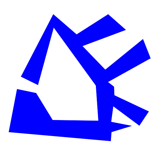


Our first result is that in , the non-contractibility does not really cause problems: the barcode of convex polygons is encoded in the barcode of the nerve of their restricted offsets, despite the presence of non-contractible intersections. The analogue statement in is not true. The result implies the existence of a linear-sized filtration, as opposed to the cubical size obtained from using the unrestricted nerves. The filtration can be computed in time , ruled by the computation time of the Voronoi diagram. While the proof ultimately still relies on the nerve theorem, it requires a deeper investigation of the structure of Voronoi diagrams of convex objects. Moreover, it requires a slight generalization of a result in [9] (see Theorem 2 below), showing that the nerve isomorphism commutes with inclusions, to the case of filtrations connected by certain simplicial maps.
Our second result is a general construction of a cell complex with the desired barcode in three dimensions. Our construction scheme computes the Voronoi diagram of the input sites as a preprocessing step and cuts (subdivides) the lower-dimensional cells of the Voronoi diagrams into smaller pieces in a controlled way. The resulting refinement of the Voronoi diagram gives rise to a dual cell complex whose size is asymptotically equal to the complexity of the Voronoi diagram of the input sites. As the latter is known to be bounded by , our filtration is significantly smaller than , as obtained by a Čech-like filtration. The time for computing the filtration is bounded from above by . The correctness proof works by (conceptually) “thicken up” lower-dimensional cells of the Voronoi diagram to obtain a good cover of the space, for which the nerve theorem applies.
We have implemented our algorithm for polygons using the Cgal library and report on extensive experimental evaluation. In particular, we compare our approach with the natural alternative to replace the input polygons with sufficiently dense point samples. Although the point sample approach yields very close approximations to the exact barcode in a comparable running time, we demonstrate that the approximation error induced by the sampling results in additional noise on a large range of scales and therefore makes the topological analysis of the offset filtration more difficult.
Related work
Since its introduction in [14], persistent homology has become an active area of research, including theoretical, algorithmic, and application results; we refer to the textbook [13] and the surveys [15, 7] for an overview. The information gathered by persistence is usually displayed either in terms of a barcode (as in this work) or, equivalently, via a persistence diagram [13].
The textbook [13] describes the most common approaches for computing filtrations of point sets, including Čech- and alpha-complexes mentioned above. Another common construction is the Vietoris-Rips complex which approximates the Čech complex in the sense that it is nested between two Čech complexes on similar scales; precisely, the Rips complex at scale contains the Čech complex at scale , and is contained in the Čech complex at scale . However, it is easy to see that this property does not carry over to the case of arbitrary convex objects.
Topological methods for shape analysis have been extensively studied: a commonly used concept are Reeb graphs which yield a skeleton representing the connectivity of the shape and can be seen as a special case of persistent homology in dimension ; see [6] for ample applications. The full theory of persistent homology has also been applied to various tasks in shape analysis, including shape segmentation [32] and partial shape similarity [16]. While these works study the intrinsic properties of a shape through descriptor functions independent of the embedding, our problem setup rather asks about extrinsic properties, that is, how the shape is embedded in ambient space.
Voronoi diagrams are one of the most basic objects in computational geometry [3, 11, 17]. Efficient algorithms for the case of point sets have been designed and implemented in 2D and 3D [27, 31, 36] and higher dimensions [21]. In the plane, generalizations to convex objects [23] and line segments and circular arcs [19, 34] have been presented. Generalizations in three dimensions include Voronoi diagrams of (infinite) lines [20] and approximating the Voronoi diagram of one polyhedron [25]. However, an exact and efficient method for a set of (convex) polyhedra in is still missing; we refer to [35] for a discussion of the difficulties.
Outline
We describe barcodes of convex objects, generalizing Čech complexes, in Section 2, introducing basic topological concepts. We define our generalization of alpha-complexes in Section 3 and show how it leads to more efficient filtrations for (Section 4) and (Section 5). We report on experimental evaluations for the planar case in Section 6. We conclude in Section 7.
2 Topological background
We review standard notation in persistent homology and dualizations of set covers through nerves. We assume familiarity with basic topological notions, in particular simplicial complexes and homology groups; the necessary background is covered by the textbook [13] and in more detail by [18, 26].
Persistent homology
A persistence module is sequence of vector spaces with linear maps for that satisfy and is the identity function on [8]. We say that is a critical value if is not isomorphic to for . We assume the usual tameness conditions that each has finite rank, and the number of critical values is finite. A generator (basis element) of is born at if for any . A generator born at dies at , if , but . In this way, every generator in is assigned to a birth-death interval and the length of the birth-death interval is called the persistence of the generator. The barcode of the persistence module is the set of these intervals.
We call a collection of spaces with the property that whenever a filtration induced by inclusion. A standard way to obtain a persistence module is to apply the homology functor on such a filtration, that is, to consider where is the -th homology group over an arbitrary fixed base field, with . Indeed, the inclusion map from to induces a map satisfying the required properties. This construction works generally for filtrations of simplicial complexes (using simplicial homology), of CW-complexes (using cellular homology) and of subsets of (using singular homology).
For simplicial complexes, we will also use a more general construction: a simplicial map between two simplicial complexes and is a map induced by mapping vertices of to vertices of . We call a sequence of simplicial complexes together with simplicial maps a filtration induced by simplicial maps. Such a filtration gives rise to a persistence module, and thus a barcode, in the same way as in the inclusion case, by applying the functor . We call the barcode of the persistence module of a filtration using the -barcode of the filtration
Nerves
Let be a collection of non-empty sets in a common domain. The underlying space is defined as . We call a non-empty subset intersecting, if . The nerve of is the collection of all intersecting subsets. It is clear by definition that every singleton set is in the nerve, and that any non-empty subset of an intersecting set is intersecting. The latter property implies that the nerve is a simplicial complex: the singleton sets are the vertices of that complex. We call a good cover if all sets in the collection are closed and triangulable, and any intersecting subset yields a contractible intersection. For example, any collection of closed convex sets forms a good cover.
Theorem 1 (Nerve Theorem).
If is a good cover, is homotopically equivalent to . In particular, for all .
The following lemma is a slightly modified version of [9, Lemma 3.4] and asserts that the isomorphisms from the nerve theorem between and commute with inclusions.
Theorem 2 (Chazal and Oudot).
Let and be good covers with for all . Then, the isomorphisms and commute with the maps and that are induced by canonical inclusions, that is, .
Barcodes of shapes
We let denote the Euclidean distance function. For a point set and , we set . Then, is called the distance function from and is called the -offset of . With as above, we write for the collection -offsets of . In particular, . We call the offset-filtration of . We pose the question of how to compute the barcode of the offset filtration of convex objects efficiently. See Figure 1 for an illustration of these concepts.
We define the analogue of Čech filtrations: We call the nerve filtration of ; it is indeed a filtration because for , .
Theorem 3.
Let be a collection of convex objects. Then, the -barcodes of offset filtration and nerve filtration of are equal for all .
Proof.
The nerve only changes for values where a collection of individual polyhedron offsets becomes intersecting. We call such an offset value nerve-critical. Since , we can restrict to collections of size at most since the -barcode is known to be trivial for (since the -th homology group is trivial for all ). Sorting the nerve-critical values and setting , the nerve filtration simplifies to the finite filtration whose barcode can be computed using standard methods; see [14, 37] or [4] for an optimized variant. Clearly, since contains a simplex for any subset of of size at most , its size is .
3 Restricted barcodes
Let be convex polyhedra in , that is, each is the intersection of finitely many half-spaces. The major disadvantage of the construction of Section 2 is the sheer size of the resulting filtration, . Our goal is to come up with a filtration that yields the same barcode and is substantially smaller in size. Our approach is reminiscent of alpha-complexes for point sets, but it requires additional ideas for being applicable to convex objects.
From now on, we make the following assumptions for simplicity: We refer to the elements of as sites. We restrict our attention to , that is, sites are polygons () or polyhedra (). We assume the sites to be pairwise disjoint and in general position, that is, for any pair of sites, there is a unique pair of points , that realizes the distance between the sites. Moreover, we assume that the number of vertices, edges and faces of each site is bounded by a constant. For a point , the site is closest if for any . We assume for simplicity the generic case that no point has more than closest sites. As a notational shortcut, we will frequently write .
The Voronoi diagram is the partition of the space into maximal connected components with the same set of closest sites. The Voronoi diagram is an arrangement in , and its combinatorial complexity is the number of cells. The Voronoi region of , denoted by , is the (closed) set of points for which is one of its closest sites. For a cell of , we call the critical value of (recall that ) and a point that attains this infimum a critical point of . Note that critical points of a cell may lie on its boundary.
For any two sites , , the bisector is the set of points that satisfy . By general position of the sites, there is a unique point on that minimizes . More generally, for , let . We will frequently use the fact that for any , is empty or contractible. This is implied by the following statement, which generalizes the well-known pseudodisk-property [24], [11, Thm.13.8]. We will prove the case in Appendix B.
Theorem 4.
For , let , be two convex disjoint polytopes in in general position and let be the unit ball. Then, is either empty, a single point, or homeomorphic to -sphere.
The restricted -offset of is defined as . We set and . In the same way as in Section 2, we define the restricted nerve filtration as and -critical values as those values where a simplex enters the restricted nerve filtration. The restricted nerve filtration can be expressed by a finite sequence of simplicial complexes that changes precisely at the -critical values. The size of the filtration is bounded by the combinatorial complexity of the Voronoi diagram. Moreover, the -critical value of a simplex associated with a Voronoi cell equals the critical value of .
![[Uncaptioned image]](1407.6132v2/non_contractible.png)
Restricting the offsets to Voronoi regions brings a problem: is not necessarily a collection of convex sets, since is not convex in general. Even worse, might not be a good cover. For instance, on the right we see three sites and the induced Voronoi diagram (in black). We see that the Voronoi regions of and intersect in two segments. This means that the proof strategy of Theorem 3 breaks down since the nerve theorem does not apply.
4 Restricted barcodes in 2D
We first restrict to the case , that means, our input sites are interior-disjoint convex polygons in the plane. While the restriction of offsets invalidates the proof of Theorem 3, it does not invalidate the statement, at least in dimensions and .
Theorem 5.
For convex polygonal sites in , the - and -barcode of the restricted nerve filtration are equal to the - and -barcode of the offset filtration, respectively.
As a consequence of this theorem, we obtain a filtration of size that has the same barcode as the offset filtration; the size follows from the fact that the complexity of the Voronoi diagram is . This is much smaller than the filtration obtained by the unrestricted nerve. The construction time is dominated by computing the Voronoi diagram and thus bounded by [34].
![[Uncaptioned image]](1407.6132v2/surrounded_regions.png)
We provide a sketch of the proof of Theorem 5, and refer the reader to Appendix A for the complete proof. We concentrate on the -barcode for the proof; the (simpler) statement for the -barcode follows with similar arguments. We first analyze more carefully what causes two restricted offsets to have a non-contractible intersection. Such a non-contractible intersection only happens when two restricted offsets intersect in several components, and thus the corresponding two sites contribute two or more bisector segments to the Voronoi diagram. This, in turn, only happens if their bisector is split by another site that “sits in-between”. Precisely, observe that the intersection of two restricted offsets consists of connected components (with ) if and only if the complement of their union induces bounded regions. We call these bounded regions surrounded region induced by the restricted offsets of two sites. A surrounded region contains at least one and potentially more sites and can therefore contain nested surrounded regions (induced by two restricted offsets within the surrounded regions). We call a surrounded region simple if it does not contain any other surrounded region. On the right, we see an example where the left and right sites induce two surrounded regions (for large enough), the upper not being simple because it contains a nested surrounded region.
Fix two sites and and assume that their restricted -offsets leave some surrounded region for some fixed . The crucial observation is that whenever this happens, is always already “filled”:
Lemma 6.
The (unrestricted) -offsets of and contain . In particular, the restricted -offsets of sites in fill out the entire region .
Proof.
Let and denote the boundary curves of and . Let , denote the points on the boundary of that lie in . Assume wlog that . The bisector of and has a segment within that connects and . Since sublevel sets on the bisector are connected, we have that for all on that bisector segment. Moreover, for any on the part of that bounds , we must have as well. Combining these two properties, the “half-region” of bounded by and the bisector segment satisfies on its boundary and by convexity of the distance function, in the whole region. Applying the same argument on the other half-region, we get the result. ∎
For a fixed , we call a site surrounded if it lies in some surrounded region, and free otherwise. Recall that we write for the restricted -offsets of the sites, and we let denote the restricted -offsets of the free sites. The previous lemma implies that disregarding the surrounded sites does not change the offset, so . Moreover, the free sites form a good cover because all surrounded regions have been removed by construction. It follows that the nerve theorem applies and for all .
The first major technical result is that . Combined with the previous statement, this implies that for any , the first homology group of the restricted -offsets is isomorphic to the first homology group of its nerve. The construction of the isomorphism is iterative, always removing the sites in an innermost, and thus simple, surrounded region at a time. Let us denote by the set of sites that are not removed yet. Initially, is the set of all sites and at the end, is the set of free sites. Let us fix a simple surrounded region , and let , be the sites surrounding it. Let be the sites within and let . We define a map from to that maps all sites in to , and each remaining site to itself. This map assigns vertices of to vertices of , and induces a simplicial map between the nerves because separates from all other sites in the nerve. Being a simplicial map, induces a map of homology groups.
Lemma 7.
is an isomorphism.
Proof.
We set and argue that : We can restrict and to a neighborhood around without changing the nerve. Since is simple, is “almost” a good cover – the only obstacle is that and intersect in two components. However, we can cut one of the two intersections open. This will cause at most one triangle in the nerve to be removed (losing this triangle is the reason why the statement does not extend to ). However, since is filled, the underlying space is a disk even after the cut, and the nerve theorem asserts that .
The proof works now by fixing a cycle in and transforming it to a cycle that does not contain any element of anymore. The idea is to “reroute” any path that enters such that it runs entirely in . Because the nerve of has trivial -homology, such a rerouting does not change the homology of the cycle. We skip further details of this elementary construction. ∎
It follows that our construction yields a sequence of isomorphisms connecting and , thus proving the equivalence of the -homology for every . This statement, however, does not immediately imply the equivalence of the -barcodes of both, because it is not clear that the constructed isomorphisms commute with inclusion. This is the second major technical result needed for the proof. With , we have the diagram
where is the isomorphism from the nerve theorem and a composition of the isomorphisms between the nerves as constructed above. The first and the third square commute as one can easily verify. The difficulty lies in the the middle square. Note that Theorem 2 does not apply here because the nerve filtration of free sites is not induced by inclusion. Indeed, when increases, sites may change their status from free to surrounded, and thus disappear from the set . However, the map as defined above induces a natural simplicial map, so the nerves of free sites form a filtration induced by simplicial maps. The remainder of the proof consists of investigating the internals of the nerve isomorphism, similar to the proof of [9, Lemma 3.4], and to show that it commutes with the simplicial map (on the level of chain groups). We skip further details. With the commutativity of the diagram, Theorem 5 follows from the persistence equivalence theorem [13, p.159].

Theorem 5 does not generalize to the -barcode. For instance, in Figure 2, we see four sites in where every triple of Voronoi regions intersects, but there is no common intersection of all four of them. Consequently, their nerve consists of the four boundary triangles of a tetrahedron and therefore carries non-trivial -homology. We refer to such homology classes as “ghost features”. In the planar case, the offset filtration can clearly not form any void (a -dimensional hole) and we can therefore safely ignore all ghosts. In , however, the -barcode carries information about the offset and the ghosts need to be distinguished from real features. At first glance, one might hope that ghost features have infinite persistence (as opposed to real features). However, we can quite easily extend the situation of Figure 2 to four prisms in that create a ghost with finite persistence This shows that considering only the nerve is problematic in dimensions higher than .
5 Restricted barcodes in 3D
As Theorem 5 does not generalize to higher-dimensions, we now present a refinement of the nerve construction for three-dimensional space. Reconsidering the “ghost example” from Section 3, it seems attractive to pass to the multi-nerve [12], that is, introducing a distinct simplex for each lower-dimensional cell of the Voronoi diagram. However, this approach is not sufficient for two reasons:
1. Voronoi cells might be non-simply connected; 2. even if the Voronoi cells form a good cover, this may not be true for the restricted offsets at all scales .See Figure 3 for an illustration.

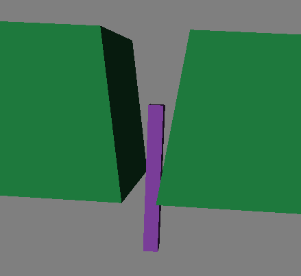
We use the following definitions: an arrangement in is a refinement of in if every -, -, -, or -dimensional cell of is contained in a cell of . For a cell and , define the restricted cell . We call stratified if for all , is empty or contractible. Note that in particular, a stratified cell is contractible. We call an arrangement a stratified refinement of , if is a refinement of and every cell of is stratified. As before, we define the critical value of a cell as .
Co-arrangements
An arrangement in gives rise to a dual structure in a natural way: fixing two cells of with , we have that either is contained in or completely disjoint from the boundary of . In the former case, we say that is incident to . If is incident to , . The of is defined as follows: for every cell of , has a co-cell such that their dimensions add up to . The boundary of a co-cell of dimension , , is the set of all co-cells of dimension such that is incident to . See Figure 4 (left) for an illustration of the corresponding concept in the planar case.

The critical value of a co-cell is defined as the critical value of its primal counterpart. This turns the co-arrangement into a filtered cell complex, since any co-cell has a critical value not smaller than any co-cell in its boundary. For , we let denote the collection of co-cells with critical value at most . Since for any , there is a well-defined homology group for each , and therefore, a barcode of the co-arrangement (equivalently, we could apply the cohomology functor on the cofiltration ). We can now state the main result which allows us to express the barcode of the offset of three-dimensional shapes as well, in terms of a combinatorial structure.
Theorem 8.
Let be a collection of convex polyhedra in , and let be a stratified refinement of . Then, the barcode of the offset filtration of equals the barcode of .
Proof.
For each cell , we define a thickening of by transforming into a -dimensional cell. The construction yields a collection of thickenings which are closed and interior-disjoint. The construction idea is to define the thickening of by an offset of with a sufficiently small radius. More precisely, we choose radii and proceed in increasing dimensions. The thickening of an -cell is its -offsets, restricted to the space that has not been occupied yet by thickenings of lower-dimensional cells. Choosing small enough and , we can ensure that two thickenings intersect if and only if the corresponding two cells are incident. More generally, a set of thickenings has a non-empty common intersection if and only the involved cells form a flag, that is, is incident to for . Finally, for sufficiently small , the intersection of such a thickened flag has a homotopy-preserving deformation to , the lowest dimensional cell of the flag. Since all cells are contractible, this implies that the thickenings form a good cover. We define as the collection of the thickening of all cells in . See Figure 4 (middle) for an illustration. For any , we define the -thickening as the subset consisting of all thickenings of cells of with a critical value of at most . forms a good cover as well just because it is a subset of the good cover . Recall that denotes the underlying space of .
The first part of the proof is to show that the filtration has the same barcode as the offset filtration . For that, we define a continuous transformation from to through a sequence of expansions and retractions. This transformation ensures that the spaces are homotopically equivalent (more formally the intersection is a deformation retract for both spaces). To construct the deformation, we let denote the deformed shape; initially, equals . We proceed in two phases, a retraction phase and an expansion phase. For a fixed , we call a cell active if , and inactive otherwise.
For the retraction phase, let be an inactive cell. Being inactive, the -offset did not reach a point on yet – however, may well intersect the thickening of already, because the offset of several sites are coming very close to (with and , such an event occurs only in the small range ). The whole purpose of the retraction phase is to remove such features from , such that has no points inside the thickenings of inactive cells empty. The retraction works as follows: let be a threshold value, starting at and continuously decreasing towards zero. The restriction of the distance function to an inactive cell induces decreasing sublevel sets with respect to threshold . This defines a retraction path for every point which has to hit the boundary, where it either stops (if we reach the boundary of an active cell) or further retracts (otherwise). Since this operation does not affect any point on any cell (active or inactive), no tearing is happening, thus the transformation is a deformation retract.
The expansion works similarly in the other direction. We let progress from towards . We let grow within each active cell simultaneously by increasing the sublevel set threshold with respect to (in informal terms, for active cells, antedates the changes happening in the cell in the future and performs them at scale all at once). Unlike in the retraction phase, this operation affects points on cells and we have to ensure that no unwanted gluing occurs. However, since is active, there is at least one point on in initially, for threshold value . Since by assumption, the sublevel set stays contractible, we are only expanding existing intersection patterns, which is enough to argue that the deformation preserves the homotopy type. At the end of the expansion, is precisely the union of all active cells, thus equal to . Also, the constructed deformations commute with inclusion on a homotopy level. Consequently, the two filtrations have the same barcode, which concludes the first part of the proof.
By duality, the flags of equal the flags of in the sense that any flag of is in one-to-one correspondence to a sequence of co-cells such that is a face of for . That implies that the nerve of the -thickenings equals the (abstract) barycentric subdivision of . Since the -thickenings are a good cover, the filtrations and have the same barcode. Putting everything together, the barcode of the offsets has the same barcode as the barycentric subdivision filtration of .
To finish the proof, it suffices to argue that the barcode of and its barycentric subdivision coincide. Note has a natural geometric realization in as the dual of an arrangement in . Moreover, its barycentric subdivision permits the same geometric realization, by picking one point in the interior of each cell and subdividing according to incidence relations. We can furthermore note that both the arrangements and the co-arrangements are CW-complexes. Since cellular and singular homology coincide for this class of complexes, the two complexes have the same homology. The argument also holds for any and the underlying map commutes with inclusions. This shows the equality of the barcodes and proves the theorem. ∎
Stratified refinements
We are left with the question of how to obtain a stratified refinement of a Voronoi diagram of convex polyhedra. We remark that for the case , the Voronoi diagram of convex polygons is already stratified, so no refinement is needed. This follows directly from the pseudodisk property (Theorem 4), ensuring that the sublevel set of each bisector stays connected for each . The resulting co-arrangement is precisely the multi-nerve as defined in [12]. However, we note that in light of Theorem 5, there is no need to consider co-arrangements at all in the planar case.
We turn to the case . Here, the Voronoi diagram is generally not stratified, for the reasons given at the beginning of the section. To stratify, we will cut every cell into stratified pieces. We consider the case of a single connected component of a bisector (that is, a -cell of the Voronoi diagram) in isolation: as it will turn out, our stratification method will ensure that all trisectors (i.e., points with the same distance to three sites) on its boundary will become stratified as well.
So, let us fix a -cell , contained in the bisector of two sites . The boundary of consists of a collection of -cells where each -cell belongs to a trisector. The boundary splits into connected components; since is homeomorphic to a plane, we can distinguish between an outer boundary of (which might be unbounded if is unbounded) and an arbitrary number of closed inner boundaries. The presence of inner boundaries turns non-simply connected, and thus is non-stratified (an example is given by Figure 3 (left)).
Note that for , we have that by definition. Therefore, cannot have more than one local minimum in the interior of since two such minima would imply two minima on the bisector, which is impossible by Theorem 4. However, it is well possible that restricted to has local minima on , both on inner and outer boundary components. The presence of such local minima turns the restricted cell disconnected for a certain range of scales and turns non-stratified as well (Figure 3 (right)).
We now define a stratified refinement of into -cells by introducing cuts in . We start by cutting along a curve on that goes through and that is unimodal for , that is, has a minimum at and -monotone otherwise. Moreover, we require to intersect every -cell in the boundary of only a constant number of times. Such a curve indeed exists since we can find two monotone paths from to the outer boundary that avoid all inner boundaries.
Having cut using , we introduce further cuts as follows: for any value , the -isoline is the curve defined by all points on the bisector with . By Theorem 4, a -isoline is a closed cycle on the bisector that loops around . Restricting to , we get that attains local maxima and minima at points on the (inner and outer) boundary curves, which we refer to as critical points. For a critical point with , an isoline segment at is a maximal connected piece of the -isoline within with on its boundary. An isoline segment may degenerate into a point. We introduce cuts along all isoline segments for all critical points. Since is unimodal, unbounded, and goes through , it intersects any isoline twice. Hence, isoline segments cannot be closed curves. An illustration is shown in Figure 5. Let be any cell of the obtained refinement of .
Lemma 9.
Any sublevel set of a refined cell is contractible.
Proof.
Fix a cell and consider restricted to . cannot have any (local) minimum in its interior, since such a local minimum would be a local minimum of the bisector and thus must be equal to . However, cuts through , so is not in the interior of any cell. Let be a point with minimal -value in . must lie on some (possibly degenerate) isoline segment because otherwise, would lie either on a segment of (which is -monotone) or on the boundary of (which we have cut into -monotone pieces). Following the boundary of , the neighboring segments of are two monotone curves , (in fact, the neighbor of might also be the second isoline segment emanating from the same critical in which case we consider to be their union).
We sweep an isoline segment in a -increasing direction which is anchored at points on and , starting with . This traces out a subset of with the property that every sublevel set is contractible. There are three cases possible:
1. and intersect in which case is bounded by , and . 2. the sweep isoline segment hits a point that is not in the interior of . Then, it follows that this intersection point must lie on an isoline segment as well (it cannot lie on a monotone curve by minimality of the isovalue). By construction, connects and 3. if none of the first two cases arise, is unbounded.In all cases, we observe that the sweeping process traces out the entire set , which implies that every sublevel set is contractible. ∎
The cuts induce a subdivision of the -cells as well. It is easy to see that no refined -cell can be a cycle – any closed curve is cut at its maxima and minima, and newly introduced isoline segments cannot not form a cycle. Therefore, all -cells in are simply-connected as well. This implies that the construction yields a stratified refinement of the Voronoi diagram.
Size of the stratified refinements
The described refinement only increases the complexity of the arrangement by a constant factor, as we shall now show. Recall that a trisector is the curve of points that have the same distance to three sites. The distance function restricted to a trisector defines a function on this curve. In the refinement procedure, we consider the local extrema of this curve. We first show the following statement.
Lemma 10.
The number of local extrema of a trisector is in .
Proof.
A trisector is defined as the set of points of equal distance to three polyhedra. Each such point is of equal distance to a face, an edge or a vertex of each of the polyhedra. This implies that a trisector of polyhedra is composed of pieces of trisectors of points, lines, and planes that support the appropriate features of the polyhedra. Each such trisector can be defined by a set of algebraic equations of constant degree, using the squared distances from a point to a point, a line, or a plane in . Maximizing or minimizing the (squared) distance function on such a trisector can be phrased as a Lagrange optimization problem with objective function and constraints being algebraic curves of constant degree. In this case, the condition of being a maximum can again be expressed as an algebraic equation of constant degree, defining a surface. Cutting this surface with the trisector yields a constant number of points, assuming that the sites are in generic position. ∎
With that lemma, it is straight-forward to prove the size bound
Theorem 11.
For a set of convex, disjoint polyhedra in generic position, let be the complexity of . Then, there exists a stratified refinement of with cells.
Proof.
We charge the cuts of a cell to - and -cells on its boundary. We start with the cuts introduced by : every such cut is between two -cells, and we can charge the cut to either of them (if cuts through a -cell, we can charge the cut to one of the incident -cells on the boundary). Since a -cell can only participate in the boundary of three -cells, and we assume that hits any -cell only a constant number of times, every -cell is charged a constant number of times. Note that a cut only introduces a constant number of new cells in the arrangement, so the complexity stays the same after all cuts induced by the -curves.
Any isoline cut on the boundary of is triggered by a local extremum at some boundary component. We charge the cut to the - or -cell that belongs to. Note that every vertex is charged for at most isoline cuts, because the vertex can only participate in bisectors, and thus, -cells. Each -cell is only charged a constant number of times, according to Lemma 10, because we cut at most times for every local extremum of the trisector that contains the -cell. Since each isoline segment induces only a constant number of additional cells, every cut can be charged to a Voronoi cell and every cell is charged only a constant number of times, we obtain the result. ∎
Together with Theorem 8, it follows that we can find a cellular filtration of size whose barcode equals the barcode of the original offset filtration. The exact value of is far from being settled but we know that it is bounded from below by (by a straightforward construction even for n points) and from above by [1, 29], so that the obtained filtration is significantly smaller than the unrestricted nerve filtration of size .
Efficient computation of the stratified refinement
We describe the procedure for constructing a refined stratification. We assume that the following primitives are readily available:
1. obtaining all critical values on a trisector; 2. finding intersection points of an isoline and a boundary curve; and 3. a boolean primitive defining a consistent order of any two points on a given isoline.As a preprocessing step we cut all boundary curves so that they are -monotone. Since the number of critical values on a trisector is constant, and using the same arguments as before, we get that the first primitive can be performed in constant time. The same holds for the second primitive, as we make sure that boundary curves are -monotone. Since an isoline is a closed curve, the third primitive can be performed by fixing a reference point on the isoline, and then, given any two points, decide according to their clockwise order from the reference point. As each isoline is composed of a constant number of curves (by our assumption that each polyhedra is of constant size), the operation can be performed in constant time.
Fixing a cell , the algorithm uses a sweep-line approach by sweeping an isoline through . For each critical point , let its critical value be . We sort all critical points according to their critical values, and go over the critical points in an increasing order. As the sweep progresses, we maintain a list of boundary curves that the sweep isoline is currently intersecting. The key observation is that when the sweep progresses between two isolines, and since the boundary curves do not intersect in their interior, the order of intersection points of the boundary curves with the isolines remains the same, with the exception that it might get shifted. However, we can fix the reference point in the third primitive so that it remains consistent with respect to the order on the previous isolines. This allows for efficient lookup, insertion, and deletion of curves by maintaining a balanced search tree of the curves, sorted by the third primitive.
The algorithm runs in two stages. The first stage creates the unbounded curve by simulating combinatorially a curve that has the desired properties, namely, that it is an unbounded curve that attains a minimum in and that is monotone otherwise. Note that is composed of two -monotone unbounded segments. We describe how to simulate a single segment using a sweep, and will repeat the procedure for the creation of the two segments. We start by picking a random intersection point for on the first isoline that we encounter in the sweep. Then, at the next isoline, we assume that acts monotonously and pick a random intersection point such that does not intersect any curve in the tree. For example, if the current intersection point is located between curves and at the current isoline, then we pick the next intersection point so that it is still located between and on the next isoline. We update the arrangement according to the choice of points by splitting the face in which the curve passes. A problem may occur when and merge, but as this must happen at a critical point, we can simply assume that intersects both and at that critical point, and update the arrangement accordingly. At the end of the process we obtain an arrangement that contains all the combinatorial information for the cuts induced by . Note that as each new edge induced by attains a minimum over in its lower endpoint, we also have the critical value of the edge.
The second stage of the algorithm introduces the cuts that are induced by isoline segments. We again perform a sweep over . When the sweep isoline hits a critical point, we look for the two curves to the sides of the intersection point in the tree, add the isoline segment bounded by those two curves to the arrangement, and split the faces accordingly. We note that it might be that the isoline segment goes in the interior of a hole. In order to handle such cases, we keep track for any two consecutive curves in the tree whether the area between them belongs to the interior of or not.
Notice that each sweep goes over critical values. At each critical value, a constant number of lookups, insertions and deletions is performed on the balanced search tree of curves. Also, the size of the tree is bounded by the size of the Voronoi diagram. Therefore, for each critical value, we perform operations, obtaining the following result.
Theorem 12.
The offset filtration of convex, disjoint polyhedra in generic position can be computed in time , excluding the computation time of the Voronoi diagram.
Together with the result of [1], we obtain an upper bound of on the expected time.
6 Convex shapes vs. point samples: Experimental comparison
Computing Voronoi diagrams of polyhedra in space is a difficult problem. While efforts to compute it are underway, so far only restricted cases have been completed; see e.g., [20]. We therefore restrict our experiments to the planar case. Still, we show that already in the plane approximating the shapes by point samples introduces noise that is hard to distinguish from real small features.
Implementation details
We implemented the restricted nerve algorithm for the two-dimensional case as described in Section 4. The algorithm requires computing the combinatorial structure of the Voronoi diagram, and the critical value of each feature of the diagram, namely what is the point on the feature that attains the minimal distance to the sites defining the feature. We solve the first task by computing the Delaunay graph for all line segments belonging to the input polygons, using Cgal’s 2D Segment Delaunay Graphs package [22]. We restrict our attention to features of the graph for which no two defining segments belong to the same polygon and remove duplicates. For the critical values, we explicitly compute the actual curves and vertices of the Voronoi diagram and compute the minimal distance to their nearest polygonal sites.
For comparison purposes, we also implemented the unrestricted nerve filtration described in Section 2. For the computation of critical values, we proceed in a brute-force manner, that is, we take the minimum distance over all pairs or triplets of line segments of the input polygons.
We also implemented an approximation of the barcode through point samples: Fixing some , we calculate a finite point set whose Hausdorff-distance to the input polygonal shapes is at most . We achieve that by placing a grid of side length in the plane and taking as our sample the centers of all grid cells which are intersected by some input polygon. We can compute this sample efficiently by taking the Minkowski sum of each polygon and a square with side length , and performing batch point location queries for a grid of points in the bounding rectangle of that polygon. We compute the alpha-filtration on the point samples, using Cgal’s 2D Triangulation package [36]. The size of the resulting filtration is linear in the number of sampled points.
In all variants, after computing the filtration, we obtain the barcode using the PHAT library [5].
Time analysis
| Number of vertices | ||||||
| Approach | ||||||
| Restricted nerve | Filtration time | 0.042 | 0.237 | 1.285 | 2.716 | 5.693 |
| Persistence time | 0 | 0 | 0 | 0 | 0 | |
| Total time | 0.042 | 0.237 | 1.285 | 2.716 | 5.693 | |
| Filtration size | 45 | 267 | 1473 | 2963 | 5949 | |
| Unrestricted nerve | Filtration time | 0.602 | 69.13 | 9920 | - | - |
| Persistence time | 0 | 0.033 | 23.11 | - | - | |
| Total time | 0.602 | 69.16 | 9943 | - | - | |
| Filtration size | 175 | 20875 | 2604375 | - | - | |
| Point sample () | Filtration time | 0.013 | 0.047 | 0.217 | 0.435 | 0.805 |
| Persistence time | 0 | 0 | 0.001 | 0.001 | 0.003 | |
| Total time | 0.013 | 0.047 | 0.217 | 0.437 | 0.808 | |
| Filtration size | 803 | 2101 | 9021 | 14235 | 22393 | |
| Point sample () | Filtration time | 0.023 | 0.07 | 0.312 | 0.594 | 1.045 |
| Persistence time | 0 | 0 | 0.003 | 0.006 | 0.01 | |
| Total time | 0.024 | 0.07 | 0.315 | 0.6 | 1.055 | |
| Filtration size | 2577 | 6707 | 28273 | 45635 | 72275 | |
| Point sample () | Filtration time | 0.304 | 0.765 | 3.22 | 5.106 | 7.975 |
| Persistence time | 0.007 | 0.016 | 0.081 | 0.132 | 0.213 | |
| Total time | 0.310 | 0.781 | 3.3 | 5.238 | 8.188 | |
| Filtration size | 48741 | 120359 | 505833 | 792395 | 1226827 | |
We compare the three approaches for several inputs of increasing sizes, and report on their running times and the size of the filtration. For generating the input, we considered a square of side length 100. We added random polygons inside the square using the following repetitive process. We randomly pick a point inside the square, and create a rectangle centered at that point with a random width and height. We then randomly select 5 points inside that rectangle and take the polygon to be their convex hull. If the polygon does not intersect any of the polygons that were previously added, we add it to our input. An illustration of an input is shown in Figure 6. All experiments were run on a 3.4GHz Intel Core i5 processor with 8GB of memory.
The experimental results are shown in Table 1. We observe that computing the filtration takes much more time than converting the filtration into a barcode. This is in sync with the common observation that despite the worst-case cubical complexity, the barcode computation scales well in practice. Moreover, we get the expected result that the unrestricted nerve yields large filtrations and high running times compared to the restricted nerve approach. In particular, for sufficiently large inputs, the time to compute the barcode from the unrestricted filtration is an order of magnitude higher than the total time in the restricted case, so even a smarter way for computing critical values will not be helpful.
Comparing the running time of the restricted nerve approach with that of the point sampling approach is difficult as it depends on the choice of . What approximation quality is reasonable generally depends on the application and the input at hand. However, we can observe that the overhead of computing the Voronoi diagrams of convex polygons instead of points is rather small, and we get the exact barcode in the same time as it would take to compute a “reasonable” approximation of the input. Of course, it should be admitted that our simple point-sampling approach could be significantly improved by sampling only the boundary of polygons instead, and even more by making the sample density adaptive to the local feature size [28] of the polygons. This however would require post-processing of the barcode to filter out topological features in the interior of polygons.
Quality of the barcodes


The barcode obtained using the point sampling approach approximates the actual barcode of the input. The stability theorem [10] ensures that the two barcodes have a distance of at most . Still, the question arises how much noise is introduced by the approximation. We remind the reader about our motivation to produce barcodes of shape: We want to identify offset values that minimize the number of short-lived homological features. Figure 6 shows an exact barcode and an approximated barcode for the same input. We see that the exact barcode contains some short bars throughout the entire barcode. The approximated barcode contains many more such bars, some originating from real features in the input, and some are artifacts of the approximation. It seems (at best) very difficult to identify the real features from the approximate barcode, which speaks in favor of using the exact approach that we have taken in this paper in such types of applications.
7 Conclusion
In this paper, we have defined cellular filtrations that yield the same barcode as the offset filtrations of convex polygons in , and convex polyhedra in . Our filtrations generalize the alpha filtrations for point sets and have a size proportional to the size of the Voronoi diagram of the involved sites. While the approach in simply consists of taking the nerve of the Voronoi regions, we had to cut lower-dimensional cells in to obtain such a filtration.
We restrict to the case of disjoint polyhedra for simplicity; in the light of our intended application to 3D printing, an extension to interior-disjoint polyhedra is desirable. Assuming disjointness, however, is not a serious restriction, as we can conceptually think of each polyhedron to be shrunk by an infinitesimal value, yielding a barcode that is arbitrarily close to the exact one. The details of this approach are left for an extended version of this paper.
We suspect that our approach from Section 5 generalizes to for and yields a filtration of same asymptotic complexity as the Voronoi diagram (for a constant dimension ). The proof of this statement, however, requires several non-trivial extensions of our results, for instance, a generalization of pseudodisk property (Theorem 4) in arbitrary dimensions.
We are in the process of implementing our refinement approach for the case of lines in , using the implementation of [20]. An interesting question in this context is whether for this special case, the Voronoi diagram is already stratified. It is not even clear to us whether in this case, an analogue of Theorem 5 holds, that is, whether the the nerve of the Voronoi regions yields an equivalent filtration.
Acknowledgment
The authors thank Micha Sharir for suggesting the outline of a proof of the pseudo-sphere property in three-dimensional space. The authors thank Michael Sagraloff for helpful discussions during this work.
References
- [1] P. Agarwal, B. Aronov, and M. Sharir. Computing envelopes in four dimensions with applications. SIAM J. Comput, 26:348–358, 1997.
- [2] P. Agarwal and M. Sharir. Pipes, cigars, and kreplach: The union of Minkowski sums in three dimensions. Disc. Comput. Geom., pages 645–685, 2000.
- [3] F. Aurenhammer and R. Klein. Chapter 5 - voronoi diagrams. In J.-R. Sack and J. Urrutia, editors, Handbook of Computational Geometry, pages 201 – 290. North-Holland, 2000.
- [4] U. Bauer, M. Kerber, and J. Reininghaus. Clear and compress: Computing persistent homology in chunks. In Topological Methods in Data Analysis and Visualization III. Springer, 2014.
- [5] U. Bauer, M. Kerber, J. Reininghaus, and H. Wagner. Phat - persistent homology algorithms toolbox. In 4th International Congress of Math. Software, 2014.
- [6] S. Biasotti, D. Giorgi, M. Spagnuolo, and B. Falcidieno. Reeb graphs for shape analysis and applications. Theoretical Computer Science, 392:5 – 22, 2008.
- [7] G. Carlsson. Topology and data. Bulletin of the Amer. Math. Soc., 46:255–308, 2009.
- [8] F. Chazal, D. Cohen-Steiner, M. Glisse, L. Guibas, and S. Oudot. Proximity of persistence modules and their diagrams. In Proc. of the 25th ACM Symp. on Comput. Geom., pages 237–246, 2009.
- [9] F. Chazal and S. Oudot. Towards persistence-based reconstruction in Euclidean spaces. In Proc. of the Twenty-fourth Annual Symp. on Comput. Geom., pages 232–241, 2008.
- [10] D. Cohen-Steiner, H. Edelsbrunner, and J. Harer. Stability of persistence diagrams. Disc. Comput. Geom., 37:103–120, 2007.
- [11] M. de Berg, M. van Kreveld, M. Overmars, and O. Schwarzkopf. Computational Geometry: Algorithms and Applications. Springer, 2nd edition, 2000.
- [12] É. Colin de Verdière, G. Ginot, and X. Goaoc. Multinerves and Helly numbers of acyclic families. In Proc. of the 28th ACM Symp. on Comput. Geom., pages 209–218, 2012.
- [13] H. Edelsbrunner and J. Harer. Computational Topology. An Introduction. Amer. Math. Soc., 2010.
- [14] H. Edelsbrunner, D. Letscher, and A. Zomorodian. Topological persistence and simplification. Disc. Comput. Geom., 28(4):511–533, 2002.
- [15] H. Edelsbrunner and D. Morozov. Persistent homology: Theory and practice. In Proc. of the Eur. Congress of Mathematics, pages 31–50, 2012.
- [16] B. Di Fabio and C. Landi. Persistent homology and partial similarity of shapes. Pattern Recognition Letters, 33(11):1445–1450, 2012.
- [17] S. Fortune. Voronoi diagrams and Delaunay triangulations. In Jacob E. Goodman and Joseph O’Rourke, editors, Handbook of Discrete and Computational Geometry, chapter 20, pages 377–388. CRC Press LLC, 1997.
- [18] A. Hatcher. Algebraic Topology. Cambridge University Press, 2001.
- [19] M. Held. Vroni and arcvroni: Software for and applications of Voronoi diagrams in science and engineering. In Voronoi Diagrams in Science and Engineering, pages 3–12, 2011.
- [20] M. Hemmer, O. Setter, and D. Halperin. Constructing the exact Voronoi diagram of arbitrary lines in three-dimensional space - with fast point-location. In Eur. Symp. on Alg., pages 398–409, 2010.
- [21] S. Hornus and J-D. Boissonnat. An efficient implementation of Delaunay triangulations in medium dimensions. Technical report, INRIA No. 6743, 2008.
- [22] M. Karavelas. 2D segment Delaunay graphs. In CGAL User and Reference Manual. CGAL Editorial Board, 4.4 edition, 2000.
- [23] M. Karavelas and M. Yvinec. The Voronoi diagram of planar convex objects. In Eur. Symp. on Alg., pages 337–348, 2003.
- [24] K. Kedem, R. Livne, J. Pach, and M. Sharir. On the union of Jordan regions and collision-free translational motion amidst polygonal obstacles. Disc. Comput. Geom., 1:59–70, 1986.
- [25] V. Milenkovic. Robust construction of the Voronoi diagram of a polyhedron. In Proc. of the 5th Canadian Conference on Comput. Geom., pages 473–478, 1993.
- [26] J.R. Munkres. Elements of algebraic topology. Westview Press, 1984.
- [27] S. Pion and M. Teillaud. 3D triangulations. In CGAL User and Reference Manual. CGAL Editorial Board, 4.4 edition, 2000.
- [28] J. Ruppert. A Delaunay refinement algorithm for quality 2-dimensional mesh generation. J. of Alg., 18(3):548 – 585, 1995.
- [29] M. Sharir. Almost tight upper bounds for lower envelopes in higher dimensions. Disc. Comput. Geom., 12(1):327–345, 1994.
- [30] M. Sharir. Private communication, 2014.
- [31] J. Shewchuk. Delaunay refinement algorithms for triangular mesh generation. Comput. Geom.: Theory and Applications, 22(1-3):21–74, 2002.
- [32] P. Skraba, M. Ovsjanikov, F. Chazal, and L. Guibas. Persistence-based segmentation of deformable shapes. In Computer Vision and Pattern Recognition Workshops, pages 2146–2153, 2010.
- [33] O. Stava, J. Vanek, B. Benes, N. Carr, and R. Mech. Stress relief: improving structural strength of 3d printable objects. ACM Transactions on Graphics, 31(4):48, 2012.
- [34] C. Yap. An O(n logn) algorithm for the Voronoi diagram of a set of simple curve segments. Disc. Comput. Geom., 2:365–393, 1987.
- [35] C.K. Yap, V. Sharma, and Jyh-Ming Lien. Towards exact numerical Voronoi diagrams. In Voronoi Diagrams in Science and Engineering, pages 2–16, 2012.
- [36] M. Yvinec. 2D triangulations. In CGAL User and Reference Manual. CGAL Editorial Board, 4.4 edition, 2000.
- [37] A. Zomorodian and G. Carlsson. Computing persistent homology. Disc. Comput. Geom., 33:249–274, 2005.
Appendix A Proof of Theorem 5: Tisk-theory
The main goal of this section is to give a proof of Theorem 5.
For that, we first slightly abstract from offsets and Voronoi regions, and define a class of objects that includes all of them.
Definition 13.
A piecewise-algebraic path is a simple path in which consists of a finite number of arcs, where each arc is a semi-algebraic curve. A piecewise-algebraic loop is such a path that is homeomorphic to a circle. A set is a bounded tisk if is the closed bounded region induced by a piecewise-algebraic loop. is an unbounded tisk if it is the closed region induced by an unbounded piecewise-algebraic path. Two tisks , with boundary curves , , are called interior-disjoint if .
We remark that every Voronoi region as well as any restricted offset is a tisk, because their boundaries consist of line segments, circular arcs, and parabolic arcs.
We consider the intersection of two interior-disjoint tisks and . Let and denote the boundary curves of and of respectively. The curve is partitioned into interior-disjoint segments, alternating between segments that belong to (such a segment may degenerate to a point), and segments that belong to . The symmetric property holds for . The partition points are denoted by . Note that is empty if and only if and are non-intersecting, or both are unbounded and their union is the whole space. Note also that by choosing an arbitrary orientation on or on , we can define a total order on . These definitions are illustrated in Figure 7.


Definition 14.
The connected components of are called complementary regions of . A surrounded region is a complementary region that is bounded.
Note that this definition of surrounded regions agrees with the definition given in Section 3 for the special case that tisks are Voronoi regions. Every surrounded region is a tisk whose boundary loop involves two consecutive points of connected by one segment in and one segment in . An unbounded complementary region might or might not be a tisk, depending on the whether and are bounded. For instance, if both and are bounded, there is only one unbounded complementary region, and it is the complement of a tisk. We can easily see that every surrounded region of contains exactly two points of . Every unbounded complementary region contains one or two points of ; more precisely, if there is only one unbounded region, it contains two points of , and if there are two such regions, they contain one point of each. See again Figure 7 for illustrations of these concepts.
Lemma 15.
Assume that is non-empty. Then, it is contractible if and only if does not induce a surrounded region.
Proof.
“” follows directly from the definition: Assume that is non-contractible. Then, decomposes into at least two connected components, and there exist consecutive points which are connected by segments in and . The tisk enclosed by this loop is a surrounded region.
For “”, contractibility implies that consists of exactly two points, and both lie in the unbounded complementary region, so there are no points in left to form a surrounded region. ∎
Next, we consider a collection of pairwise interior-disjoint tisks. We assume generic position, that is, no more than three tisks intersect in a common point. Three tisks of with boundary curves intersect in at most two points; this follows from the observation that (because any intersection of in the interior of a segment of would imply that is not interior disjoint to or ), combined with the fact that must be contained in some complementary region of , each of which contains at most points of .

Lemma 16.
If any pair in is empty or contractible, then every triple in is empty or a single point.
Proof.
Consider a triple with boundary curves and non-empty intersection. We assume that is contractible. That implies that . Wlog, we can assume that , because otherwise, contains of at most one point and we are done. Let . There exists a segment of connecting to . Assume first that is unbounded: then, there exist two segments in , one emenating at , one at . Since cannot intersect in the interior of , must be a subset of . However, contains and , therefore, it consist of at least two connected components. This is a contradiction to the assumption that is contractible. A symmetric argument implies that must be bounded.
We are left with the case that both and are bounded. Then and are segments that connect and . Since and are contractible, it follows that the loop of is the union of these segments. However, that loop encloses both and , which contradicts the interior disjointness the tisks. ∎

For the upcoming definitions, see also Figure 9. For a surrounded region induced by and , we call a tisk in a member of if . Note that a surrounded region might have an arbitrary number of members, including no member at all. We let denote the set of members of , and the set of extended members. We call a surrounded region filled, if the union of its members equals (in this case, must have at least one member). We define a simple surrounded region of to be a surrounded region such that no other surrounded region is contained in it.
The following property will be of special importance; we will refer to it as the “guarding principle”.
Lemma 17.
For a collection of tisks in generic position and a surrounded region , there is no intersection of a member of with an element of .
Proof.
Let be induced by the tisks and , and let , their boundaries. Assume by contradiction the existence of such an intersection. Then, there must be a tisk that intersects the boundary of . It is easy to see that this intersection cannot take place within (because and are interior-disjoint and is simple), and the same way for . It follows that intersects the boundary of at . However, by assumption, intersects a fourth tisk at point . So, is an intersection of four tisks which contradicts our genericity assumption. ∎
An equivalent statement is that if is induced by and , the set constitutes a separator in , separating the elements within and the elements outside of .
We now state the first main theorem that will be needed for the proof of Theorem 5. As usual, we let denote the underlying space of , which is the union over all tisks in .
Theorem 18.
Let be a collection of tisks in generic position such that every surrounded region is filled. Then .
The idea of the proof is to “clear out” surrounded regions one after the other by removing the members within a surrounded region and charging the surrounded region to one of the two tisks that surround it. These operations do not change the underlying space. Moreover, as we will show, there cannot be any non-trivial -homology in the nerve of a surrounded region. Finally, by the guarding principle, removing the member of a surrounded region does not affect the connectivity of remaining tisks. These properties will be enough to ensure the isomorphism. We give the details of the single steps next.

Lemma 19.
Let be a surrounded region that is simple and filled. Then, .
Proof.
Let the surrounded region be induced by , and we set for notational convenience. First of all, note that we can restrict and to a local neighborhood around without changing the nerve of . Formally, replace by , which is the intersection of with an -offset of (for small enough), and same for . We set . Clearly, . See Figure 10 (middle).
We want to prove the claim using the Nerve theorem; however, the intersection of and is non-contractible. We perform another local surgery to avoid this problem: Let be one of the two intersection points of , and let be the member adjacent to this point ( exists because is filled, and is unique because only three tisks intersect in one point). We can separate and locally around with a small distance while leaving the pairwise intersections with intact (again, because we assume non-degeneracy, is a non-degenerate segment). Let , be the replacements, and let ; note that and are still connected at the second intersection point of ; it follows that has the same edges of ; in fact, the nerves are the same, except that the triangle might or might not have a counterpart in . See Figure 10 (right).
It is enough to show that . Any pair of tisks in has a non-contractible intersection: we explicitly constructed and to have non-contractible intersection, and if any pair in had a non-contractible intersection, it would introduce a surrounded region inside which contradicts the assumption that is simple. By Lemma 16, this implies is a good partition and the Nerve theorem applies. So, is homotopically equivalent to , which is a topological disk because is filled. It follows that , as required. ∎
Recall that is the set of member of a surrounded region and let denote the set . We define a map
mapping each member of to , and any other tisk to itself. We have the induced simplicial map
which maps a simplex with to the simplex . Slightly abusing notation, we also write for this map on the nerve level. Note that might be equal to , so may map a -simplex to an -simplex with .
We need to argue that is well-defined, that is, . For that, observe that if does not contain any member of , it stays in the nerve when removing , and . On the other hand, if contains any member of , it can only contain extended members of by the guarding principle. Therefore, or , and both are in .
Being a simplicial map, induces a map
of homology groups. We show that this map is an isomorphism if is simple and filled.

Lemma 20.
If a surrounded region is simple and filled, the map is an isomorphism.
Proof.
implies immediately that the map is surjective. The support of a -chain is the union of all vertices that are boundary vertices of at least one simplex in the chain. For injectivity, we claim for any -cycle in , there is an homologous cycle that is only supported by vertices in . Indeed, this statement implies injectivity: Assume that are such that . Then, we can replace the representatives , by supported by . Since is the identity on , we have
To prove the remaining claim, we fix a -cycle in . decomposes into a collection of “simple” loops, that is, loops in which every vertex is traversed only once. There are three possibilities for such a loop: Its support lies (1) entirely in , (2) entirely in , or (3) contains elements of both and . In the latter case, both and must be in the support (because and are the only entry points into from the outside by the guarding principle), and the loop splits into two parts at and , one that is supported entirely by and one entirely supported by . See also Figure 11.
We construct from as follows: Iterating over all loops of , we remove loops of type (1), and leave loops of type (2) unchanged. For loops of type (3), we replace the subpath supported by with the edge . Note that after these replacements, is indeed supported by vertices in .
It remains to prove that . We show that every loop transformation yields a homologous cycle. For type (1), note that the loop is a cycle in . By Lemma 19, such a cycle is null-homologous, so removing the loop does not change the homology type. For type (2), there is nothing to do. For type (3), consider the subpath of the loop inside ; if it consists only of the edge , the loop remains unchanged. Otherwise, the concatenation of the path with the edge induces a cycle in . Using Lemma 19, the loop is null-homologous, thus we can one path by the other without changing the homotopy type. ∎
We complete the proof of the first main statement next.

Theorem 21.
Let be a collection of tisks in generic position such that every surrounded region is filled. Then .
Proof.
We assume that induces at least one surrounded region. In that case, it must also induce a simple one, and we let denote it and be the pair in that causes . By Lemma 20, because is filled, we have . Now, we set and consider , where we replace with (Figure 12). We note that , because the extension of did not introduce any new connection. This implies in particular that Moreover, , because occupies exactly the space that has been occupied by the members of . Finally, the surrounded regions of are equal to the surrounded regions of , except that the simple region was removed. In other words, representing the surrounded region by a forest where is an ancestor of if , the surrounding forest of equals the surrounding forest of with one leaf removed.
By iterating this construction, we find a collection of tisks such that , , and does not induce any surrounding region. The last property, however, implies that all pairwise intersections are contractible. Therefore, Lemma 16 applies and we can use the Nerve Theorem, which states that is homotopically equivalent to . In particular, their homology groups are isomorophic. Putting everything together, we have that
∎
Finally, we consider filtrations of tisks according to the following definition.
Definition 22.
A family of tisks is called a tisk-inclusion if for . A collection of tisk-inclusions is called a tisk-filtration. For each , it defines a collection of tisks at scale . A tisk-filtration is called sane if for every , the collection of tisks is interior-disjoint, in generic position, and all its surrounded regions are filled.
For a sane tisk-filtration , Theorem 21 establishes an isomorphism between the first homology group of and for every . On the other hand, for , we have natural inclusions from to as well as inclusions on their nerves. We show next that these inclusions commute with the isomorphisms.
Theorem 23.
For a sane tisk-filtration and , the diagram
commutes, where is the isomorphism as constructed in Theorem 21.
Proof.
The proof is lengthy and requires us to study the isomorphisms induced by the Nerve theorem, in a similar spirit as in [9]. We let denote the the surrounded regions of and those of . Clearly, and we can label the surrounded regions such that for . Recall that in the construction of (Theorem 21), we repeatedly remove tisks from surrounded regions and charge their area to one of its surrounding tisks. After removing all surrounded regions, we arrive at a collection from with the same underlying space, and a simplicial map
which induces an isomporphism between the -st homology groups. Moreover, because has no surrounded regions, the Nerve theorem defines an isomorphism
Finally, there is a natural simplicial map
where we map a tisk that is not surrounded at , but surrounded at to one of its surrounding tisks (in other words, can be seen as the restriction of to ). Putting everything together, we have the following diagram
where means that the corresponding map is induced by inclusion. We show that every square in this diagram commutes. This is immediately clear for the upper square from the top. For the lower square, we observe that the corresponding diagram on the simplicial level already commutes, by definition of .
For the middle square, we need to investigate the isomorphism in more detail. (Note that we cannot apply Theorem 2 because is not induced by inclusion) We still want to follow the approach from [9, Lemma 3.4], [18, Sec. 4G]. A technical difficulty is that these results require open covers of the underlying space, while we cover with closed spaces. However, we can just replace any tisk in by an offset of itself with a sufficiently small -value and restrict the offset to the underlying space. This yields an open cover , with same underlying space and the same nerve as – this is possible because we assume our tisks to be bounded by finitely many algebraic sets which rules out pathological cases where tisks come arbitrary close to each other without intersecting. With that, we have the diagram
where the upper and lower square obviously commute, and we only need to show that the middle square commutes. Set for convenience, and let denote the elements in the open cover . Let denote the standard simplex of dimension . We define a space as follows: Any non-empty subset defines a simplex of choosing the corresponding vertex set. Also, induces a (possibly empty) set . We set
Our next goal is to define a map that connects and . Note first that is defined through a vertex map from one nerve to the other, by identifying surrounded tisks with one of their surrounders. By assigning indices and tisks, can be encoded as a map . Note that the individual tisks are only growing when surrounded regions are eliminated; therefore, we have that . also extends to a surjective map from to in a natural way, and we have that . Therefore, the map
which maps to is well-defined.
Finally, let denote the barycentric subdivision of and note that also extends to a map in a natural way. Now we consider the following diagram
where is the natural projection from to and is the map obtained by contracting every to a single point, say . Both squares commute: For the first square, this is immediately clear, because a point is mapped to , regardless of how to follow the diagram. For the second square, let and note that and .
We consider the diagram
of -chain groups, where , are chain maps for dimension induced by and (see [26, p.72]). is the chain map defined by mapping a -simplex to the chain of -simplices that are incident to the vertex representing in . It is again straight-forward to see that the diagram commutes: Fix a -simplex . If is contracted, that is, two of its boundary vertices are identified, every simplex of incident to is also contracted. It follows that . On the other hand, of is not contracted, every simplex in the barycentric subdivision that is incident to is mapped to a non-trivial -chain, and it is easy to verify that also in this case.
Summarizing the previous two steps, we have the commutative diagram
We apply the previous theorem on the case of restricted offset filtrations and prove Theorem 5:
Theorem 24.
For convex polygonal sites in , the - and -barcode of the restricted nerve filtration are equal to the - and -barcode of the offset filtration, respectively.
Proof.
For the -barcode, it is enough to show that the restricted offset filtration yields a sane tisk-filtration according to Definition 22. By assumption, the restricted offsets are in generic position and interior-disjoint. It remains to show that for any , any surrounded region is filled.
Consider a region surrounded by and with boundary curves and . Let , denote the points on the boundary of that lie in . Assume wlog that . We have to show that the union of the restricted -offset sites cover . For that, it suffices to show that the unrestricted -offsets of and cover , what we show next. It can easily be seen that the bisector of and has a segment within that connects and . With Theorem 4, we have that for all on that bisector segment. Moreover, for any on the part of that bounds , we must have as well. Combining these two properties, the “half-region” of bounded by and the bisector segment satisfies on its boundary and by convexity of the distance function, in the whole region. Applying the same argument on the other half-region, we get the result.
The result for the -barcode is obtained by proving that an analogue version of Lemma 20 also holds for -homology. The proof for that is similar, but simpler than for the -homology case. We omit further details. ∎
Appendix B Pseudo-disk property in three dimensions
Recall the following famous result on the intersection of Minkowski sums of convex objects [24], [11, Thm.13.8]
Theorem 25.
Let , be two convex interior-disjoint polygons and let be another convex object. Then, consists of at most points.
(Partial) extensions of the theorem have been given, for instance, in [2]. We will restrict our attention to the case that is the unit ball. In this appendix, we will prove to the following generalization to the three-dimensional case –we are indebted to Micha Sharir who sketched the basic construction idea of the proof [30].
Theorem 26.
Let , be two convex disjoint polyhedra in in general position and let be the unit ball. Then, is either empty, a single point, or homeomorphic to a closed cycle.
Proof.
Since and are convex and interior-disjoint, there is a plane that separates the interior of the two sets. We can assume w.l.o.g. that passes through the origin and that equals to -plane after a suitable translation and rotation. We assume wlog that is above and is below . We fix the unit sphere . Any point on defines a direction in . The direction defines an ordering of all planes that are normal to . We say the a plane is further than a plane if comes after when we go in direction . Let be the furthest plane normal to that intersects . The same way, is the furthest plane for . We call more extreme than in direction if is further than . We call them equally extreme if and coincide. Clearly, partitions into , the set of directions that are more extreme for , , the set of directions more extreme for , and , the directions which are equally extreme.
First of all, note that and are non-empty, because in the upwards direction , is more extreme, and in the downwards direction , is more extreme. We show that is a closed cycle. For that, note that cuts out the equator from . Letting denote a vector on the equator, let be the plane spanned by and . The projections , of , to are convex sets in the plane. Fixing a direction in , we can observe that is more extreme for than if and only if is more extreme for than for , and the same is true for equally extreme points. For the planar case, however, it is known that there are precisely equally extreme directions, cutting the unit circle into two parts, one of which gives all directions where is more extreme, and one where is more extreme. When varying , the equally extreme directions vary continuously, so the family of all such planes traces out a cycle of directions where and are equally extreme, cutting into two disks, one more extreme for and one more extreme for .
Now, consider the set . is either empty, a single point, or a -dimensional convex shape. We assume that it is -dimensional, since the statement follows easily otherwise. We consider the -expansion of , where arbitrary. Every point on originates from a unique point on ; we let denote the corresponding map. Also, is differentiable. Therefore, every point on the boundary has a unique tangent plane and an associated outward normal vector. Vice versa, every direction appears as an outward normal vector exactly once because is convex. This implies the existence of a homeomorphism . In particular, the cycle maps to a cycle on . Furthermore, for , we call a supporting direction for if is completely contained in the half-space that contains and is bounded by the plane through that is normal to . Then, is a supporting direction for if and only if there exists a such that and is the outward normal vector of .
Set . Remember that we want to show that is empty, a point, or a cycle. We argue that . Let . Therefore, by the basic properties of Minkowski sums, there exists a supported direction by such that with the most extreme point in direction. Since as well, it follows that is not more extreme than in direction . The same way, , with and also a supported direction by , and is not more extreme than in direction . Now, there exist points with and the outward normal vectors of , are and , respectively. Since is not more extreme than in direction , we have that . The same way, . If either of the points lies on , we are done. Otherwise, since the preimage of under is connected, there is a path from to in the preimage, and this path has to cross . The intersection point then asserts that . The opposite directions follows by a similar argument.
Since is continuous, the previous argument shows that is closed curve on , but we have to exclude the case that is self-intersecting. Assume for a contradiction the presence of a self-intersection at and consider a sufficiently small neighborhood around on . By assumption, there are at least arcs of leaving ; for simplicity, assume that there are precisely arcs (the argument easily extends to the case of higher singularities). These arcs cut the neighborhood into sectors. Each sector is a part of which either belongs to or to (it can not belong to both, because then, the whole sector would belong to ). By generic position, the sectors are alternating between and . Now, since is differentiable and is part of it, there is a unique tangent plane at for . The same applies for the set , and we let denote the tangent plane with respect to this set. Because of the alternating sector property, it follows that . Let be the direction normal to . It follows that there exist points and such that . This implies that , contradicting the assumption that and are disjoint. ∎