Sequential Changepoint Approach for Online Community Detection
Abstract
We present new algorithms for detecting the emergence of a community in large networks from sequential observations. The networks are modeled using Erdős-Renyi random graphs with edges forming between nodes in the community with higher probability. Based on statistical changepoint detection methodology, we develop three algorithms: the Exhaustive Search (ES), the mixture, and the Hierarchical Mixture (H-Mix) methods. Performance of these methods is evaluated by the average run length (ARL), which captures the frequency of false alarms, and the detection delay. Numerical comparisons show that the ES method performs the best; however, it is exponentially complex. The mixture method is polynomially complex by exploiting the fact that the size of the community is typically small in a large network. However, it may react to a group of active edges that do not form a community. This issue is resolved by the H-Mix method, which is based on a dendrogram decomposition of the network. We present an asymptotic analytical expression for ARL of the mixture method when the threshold is large. Numerical simulation verifies that our approximation is accurate even in the non-asymptotic regime. Hence, it can be used to determine a desired threshold efficiently. Finally, numerical examples show that the mixture and the H-Mix methods can both detect a community quickly with a lower complexity than the ES method.
I Introduction
Community detection within a network arises from a wide variety of applications, including advertisement generation to cancer detection [1, 2, 3, 4, 5]. These problems often consist of some graph which contains a community where and differ in some fundamental characteristic, such as the frequency of interaction (see [6] for more details). Often this community is assumed to be a clique, which is a network of nodes in which every two nodes are connected by an edge. Here we consider the statistical community detection problem, where the observed edges are noisy realizations of the true graph structures, i.e., the observations are random graphs.
Community detection problems can be divided into either one-shot [7, 8, 9, 10, 11] or dynamic categories [12, 13, 14]. The more commonly considered one-shot setting assumes observations from static networks. The dynamic setting is concerned with sequential observations from possibly dynamic networks, and has become increasingly important since such scenarios become prevalent in social networks [13]. These dynamic categories can be further divided into networks with (1) structures that either continuously change over time [12], or (2) structures that change abruptly after some changepoint [14], the latter of which will be the focus of this paper.
In online community detection problems, due to the real time processing requirement, we cannot simply adopt the exponentially complex algorithms, especially for large networks. Existing approaches for community detection can also be categorized into parametric [15, 16, 17, 18] and non-parametric methods [19]. However, many such methods [19, 18] rely on the data being previously collected and would not be appropriate for streaming data.
Existing online community detections algorithms are usually based on heuristics (e.g. [7]). It is also recognized in [20] that there has been tenuous theoretical research regarding the detection of communities in static networks. The community detection problem in [20] was therefore cast into a hypothesis testing framework, where the null hypothesis is the nonexistence of a community, and the alternative is the presence of a single community. They model networks using an Erdős-Renyi graph structure due to its comparability to a scale-free network. Based on this model, they derive scan statistics which rely on counting the number of edges inside a subgraph [10], and establish the fundamental detectability regions for such problems.
In this paper, we propose a sequential changepoint detection framework for detecting an abrupt emergence of a single community using sequential observations of random graphs. We also adopt the Erdős-Renyi model, but our methods differ from [10] in that we use a sequential hypothesis testing formulation and the methods are based on sequential likelihood ratios, which have statistically optimal properties. From the likelihood formulations, three sequential procedures are derived: the Exhaustive Search (ES), the mixture, and the Hierarchical Mixture (H-Mix) methods. The ES method performs the best but it is exponentially complex even if the community size is known; the mixture method is polynomially complex and exploits the fact that the size of the community inside a network is typically small. A limit of the mixture method is that it raises a false alarm due to a set of highly active edges that do not form a community. The H-Mix method addresses this problem by imposing a dendrogram decomposition of the graph. The performance of the changepoint detection procedures are evaluated using the average-run-length (ARL) and the detection delay. We derived a theoretical asymptotic approximation of the ARL of the mixture method, which was numerically verified to be accurate even in the non-asymptotic regime. Hence, the theoretical approximation can be used to determine the detection threshold efficiently. The complexity and performance of the three methods are also analyzed using numerical examples.
This paper is structured as follows. Section II contains the problem formulation. Section III presents our methods for sequential community detection. Section IV explains the theoretical analysis of the ARL of the mixture model. Section V contains numerical examples for comparing performance of various methods, and Section VI concludes the paper.
II Formulation
Assume a network with nodes and an observed sequence of adjacency matrices over time with , where represents the interaction of these nodes at time . Also assume when there is no community, there are only random interactions between all nodes in the network with relatively low frequency. There may exist an (unknown) time at which a community emerges and nodes inside the community have much higher frequencies of interaction. Figures 1 and 2 illustrate such a scenario.


We formulate this problem as a sequential changepoint detection problem. The null hypothesis is that the graph corresponding to the network at each time step is a realization of an Erdős-Renyi random graph, i.e., edges are independent Bernoulli random variables that take values of 1 with probability and values of 0 with probability . Let denote the th element of a matrix , then
The alternative hypothesis is that there exists an unknown time such that after , an unknown subset of nodes in the graph form edges between community nodes with a higher probability , :
and for all other connections
We assume that is known, as it is a baseline parameter which can be estimated from historic data. We will consider both cases when is either unknown or known. Our goal is to define a stopping rule such that for a large average-run-length (ARL) value, , the expected detection delay is minimized. Here and consecutively denote the expectation when there is no changepoint, and when the changepoint occurs at time .
III Sequential community detection
Define the following statistics for edge and assumed changepoint time for observations up to some time ,
| (10) |
Then for a given changepoint time and a community , we can write the log-likelihood ratio for (II), (II) and (II) as follows:
| (11) |
Often, the probability of two community members interacting is unknown since it typically represents an anomaly (or new information) in the network. In this case, can be replaced by its maximum likelihood estimate, which can be found by taking the derivative of (11) with respect to , setting it equal to and solving for :
| (12) |
where is the cardinality of a set . In the following procedures, whenever is unknown, we replace it with .
III-A Exhaustive Search (ES) method
First consider a simple sequential community detection procedure assuming the size of the community, , and are known. The test statistic is the maximum log likelihood ratio (11) over all possible sets and all possible changepoint locations in a time window . Here is the start and is the end of the window. This window limits the complexity of the statistic, which would grow linearly with time if a window is not used. The stopping rule is to claim there has been a community formed whenever the likelihood ratio exceeds a threshold at certain time . Let . The exhaustive search (ES) procedure is given by the following
| (13) |
where is the threshold.
Note that the testing statistic in (13) searches over all possible communities, which is exponentially complex in the size of the community . One fact that alleviates this problem is when is known, there exists a recursive way to calculate the test statistic in (13), called the CUSUM statistic [21]. For each possible , when , we calculate
| (14) |
with and the detection procedure (13) is equivalent to:
| (15) |
where is the threshold. When is unknown, however, there is no recursive formula for calculating the statistic, due to a nonlinearity resulting from substituting for .
III-B Mixture method
The mixture method avoids the exponential complexity of the ES method by introducing a simple probabilistic mixture model, which exploits the fact that typically the size of the community is small, i.e. . It is motivated by the mixture method developed for detecting a changepoint using multiple sensors [22] and detecting aligned changepoints in multiple DNA sequences [23]. The mixture method does not require knowledge of the size of the community .
We assume that each edge will happen to be a connection between two nodes inside the community with probability , and use i.i.d. Bernoulli indicator variables that take on a value of 1 when node and node are both inside the community and otherwise:
Here is a guess for the fraction of edges that belong to the community. Let
| (19) |
With such a model, the likelihood ratio can be written as
| (20) |
and the mixture method detects the community using a stopping rule:
| (21) |
where is the threshold. Here can be viewed as a soft-thresholding function [22] that selects the edges which are more likely to belong to the community.
However, one problem with a mixture method is that its statistic can be gathered from edges that do not form a community. Figure 3 below displays two scenarios where the mixture statistics will be identical, but Figure 3(b) does not correspond to a network forming a community. To solve this problem, next we introduce the hierarchical mixture method.
 |
 |
| (a) | (b) |
III-C Hierarchical Mixture method (H-Mix)
In this section, we present a hierarchical mixture method (H-Mix) that takes advantage of the low computational complexity of the mixture method in section III-B while enforcing the statistics to be calculated only over meaningful communities. Hence, the H-Mix statistic is robust to the non-community interactions displayed in Figure 3. The H-Mix method requires the knowledge (or a guess) of the size of the community .
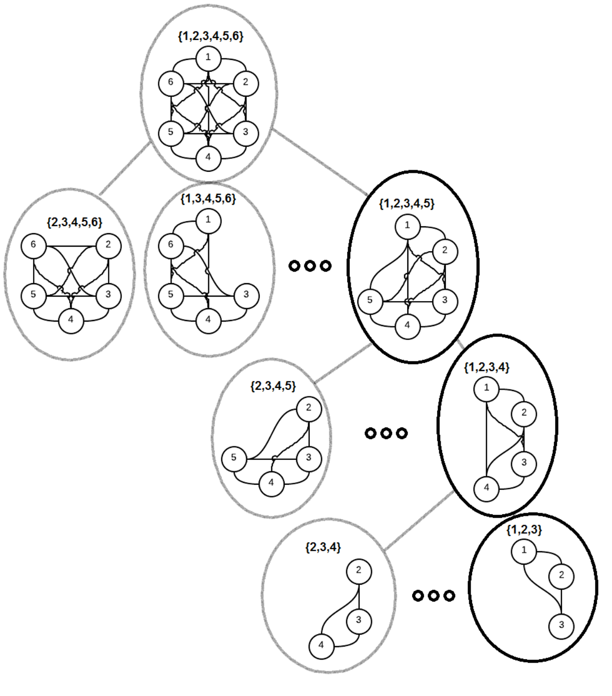
The H-Mix method enforces the community structure by constructing a dendrogram decomposition of the network, which is a hierarchical partitioning of the graphical network [24]. The hierarchical structure provided by dendrogram enables us to systematically remove nodes from being considered for the community. Suppose a network has a community of size . Starting from the root level with all nodes belonging to the community, each of the nodes in the dendrogram tree decomposition is a subgraph of the entire network that contains all but one node. Then the mixture statistic from (21) is evaluated for each subgraph: using defined in (19), for a given set of nodes and a hypothesized changepoint location , the mixture statistic is calculated as
| (22) |
We iteratively select the subgraph with the highest mixture statistic value, since it indicates that the associated node removed is most likely to be a non-member of the community and will be eliminated from subsequent steps. The algorithm repeats until there are only nodes remaining in the subgraph. Denote the mixture statistic for the selected subgraph as . Then is a series of test statistics at each hypothesized changepoint location . Finally, the H-Mix method is given by
| (23) |
where is the threshold. The idea for a dendrogram decomposition is similar to the edge removal method [2], and here we further combine it with the mixture statistic. Figure 4 illustrates the procedure described above and Algorithm 1 summarizes the H-Mix method.
III-D Complexity
| ES | ||
|---|---|---|
| Mixture | ||
| H-Mix |
In this section, the algorithm complexities will be analyzed and the complexities are summarized in Table I. The derivation of these complexities are explained as follows. Given a known subset size and at a given changepoint location and current time , evaluating the ES test statistic requires in operations. Using Stirling’s Approximation , where the entropy function is , the complexity of evaluating ES statistic is . This implies that for , the complexity will be approximately polynomial . However, a worst case scenario occurs when , as the statistic must search over the greatest number of possible networks and the complexity will consequently be which is exponential in .
The mixture method only uses the sum of all edges and therefore the complexity is . Unlike the exhaustive search algorithm, the mixture model has no dependence on the subset size , by virtue of introducing the mixture model with parameter .
On the th step, the H-Mix algorithm computes mixture statistics, and there are steps required to reduce the node set to final nodes. Therefore the total complexity is on the order of , which is further reduced to if it is assumed that .
IV Theoretical Analysis for mixture method
In this section, we present a theoretical approximation for the ARL of the mixture method when is known using techniques outlined as follows. In [23] a general expression for the tail probability of scan statistics is given, which can be used to derive the ARL of a related changepoint detection procedure. For example, in [22] a generalized form for ARL was found using the general expression in [23] . The basic idea is to relate the probability of stopping a changepoint detection procedure when there is no change, , to the tail probability of the maxima of a random field: , where is the statistic used for the changepoint detection procedure, is the threshold, and denotes the probability measure when there is no change. Hence, if we can write for some , by relying on the assumption that the stopping time is asymptotically exponentially distributed when , we can find the ARL is . However, the analysis for the mixture method here differs from that in [22] in two major aspects: (1) the detection statistics here rely on a binomial random variable, and we will use a normal random variable to approximate its distribution; (2) the change-of-variable parameter depends on and, hence, the expression for ARL will be more complicated than that in [22].
Theorem 1.
When , an upper bound to the ARL of the mixture method with known is given by:
| (24) |
and a lower bound to the ARL is given by:
| (25) |
where
| (26) |
and and denote the first and second order derivatives of a function , is a normal random variable with zero mean and unit variance, the expectation is with respect to , and the special function is given by [22]
Here is the solution to
We verify the theoretical upper and lower bounds for ARL of the mixture method versus the simulated values, and consider a case with , , and . The comparison results are shown in Figure 5, and listed in Table II. These comparisons show that the lower bound is especially a good approximation to the simulated ARL and, hence, it can be used to efficiently determine a threshold corresponding a desired ARL (which is typically set to a large number around 5000 or 10000), as shown in Table III. Figure 6 demonstrates that only small values in the integration equation (24) contribute to the sum and play a role in determining the ARL.
| (a) | (b) |
| (a) | (b) |
| Threshold | Theory LB | Theory UB | Simulated |
|---|---|---|---|
| 7.3734 | 5000 | 33878 | 6963 |
| 8.0535 | 10000 | 74309 | 14720 |
| ARL | Theory | Simulate ARL | Simulated |
|---|---|---|---|
| 5000 | 7.37 | 5049 | 7.04 |
| 10000 | 8.05 | 10210 | 7.64 |
V Numerical Examples
In this section, we compare the performance of our three methods via numerical simulations. We first use simulations to determine the threshold for each method, so these methods all have the same average run length (ARL) which is equal to 5000, and then estimate the detection delays using these ’s under different scenarios. The results are shown in Table IV, including the detection delay and the thresholds (shown in brackets). Note that the low-complexity mixture and H-Mix methods can both detect the community quickly.
| Parameters | ES | Mixture (known) | H-Mix | Mixture (unknown) |
| 3.8 (9.96) | 4.3 (6.71) | 3.8 (9.95) | 9.1 (3.03) | |
| 9.5 (10.17) | 12.8 (6.77) | 10.8 (10.18) | 12.5 (2.94) | |
| 5.0 (8.48) | 6.7 (6.88) | 6.4 (10.17) | 7.7 (2.03) |
Next, we test the case when there are a few active edges inside the network that do not form a community, as shown in Fig. 3(b). Assume the parameters are , , , and , and we set the thresholds for each method so they have the same ARL which is equal to 5000. Table V demonstrates that the ES and H-Mix methods can both identify this “false community” case by having relatively long detection delay and, hence, we can effectively rule out such “false communities” by setting a small window size . In contrast, the mixture method cannot identify a “false community” and it (falsely) raises an alarm quickly. Code for implementing theoretical calculation and simulations can be found at http://www2.isye.gatech.edu/yxie77/CommDetCode.zip.
| Method | Threshold (ARL = 5000) | Detection Delay |
|---|---|---|
| ES | 9.96 | 49.7 |
| Mixture | 6.71 | 4.3 |
| H-Mix | 9.95 | 100.7 |
VI Conclusions and Future Work
In this paper, we have presented and studied three methods for quickly detecting emergence of a community using sequential observations: the exhaustive search (ES), the mixture, and the hierarchical mixture (H-Mix) methods. These methods are derived using sequential changepoint detection methodology based on sequential likelihood ratios, and we use simple Erdős-Renyi models for the networks. The ES method has the best performance; however, it is exponentially complex and is not suitable for the quick detection of a community. The mixture method is computationally efficient, and its drawback of not being able to identify the “false community” is addressed by our H-Mix method by incorporating a dendrogram decomposition of the network. We derive accurate theoretical approximations for the average run length (ARL) of the mixture method, and also demonstrated the performance of these methods using numerical examples.
Though community detection has been the focus of this paper, locating the community within the network (community localization) can still be accomplished by the exhaustive search and hierarchical mixture methods (find the subgraph with the highest likelihood). The mixture method cannot be directly used for localizing the community.
We focused on simple Erdős-Renyi graphical models in this paper. Future work includes extending our methods to other graph models such as stochastic block models [25].
Outline of proof for Theorem 1.
We first approximate the distribution of in (10) by a normal random variable with the same mean and variance. Following (10),
Let denote the number of samples after the hypothesized changepoint location . Recall that is a Bernoulli random variable. We will approximate the distribution of by a normal random variable with the same mean and variance (when is large, by the central limit theorem this approximation will be accurate). Therefore,
| (27) |
where are i.i.d. standard normal random variables with zero mean and unit variance. Using this normal approximation, the detection statistic for the mixture method in (21) can be redefined as
| (28) |
Use the equation (3.3) in [23] for the tail probability of a sum of functions of standard normal random variables, we obtain that
| (29) |
Note that the above expression (29) can be rewritten as
| (30) |
Let . Hence
| (31) |
When is large, we can approximate this sum by an integration. We will omit the subscript of and for simplicity and recover them in the final expression (but it should be kept in mind that they depend on the variable and should be kept inside the integral). Then (30) becomes
| (32) |
Note that since is much larger than or . Using a change-of-variable
| (33) |
we have and . Plugging these into the above expression, we have that (32) becomes
| (34) |
which is linear in and a desirable result for our analysis.
On the other hand, we assume that is exponentially distributed with mean . Hence, (from Taylor expansion approximation). Therefore, . Now combine this with (34), we have the ARL is given by
| (35) |
where the last line is equal to (24). Note that is the solution to since and by our previous change-of-variable (31) and (33). This expression can be used as an upper bound to the ARL since it replaces a sum with integral.
References
- [1] S. Fortunato, “Community detection in graphs,” Phys. Rep., vol. 486, pp. 75–174, Feb 2010.
- [2] M. Newman, “Detecting community structure in networks,” Euro. Phys. Jour. B - Condensed Matter and Complex Systems, vol. 38, pp. 321–330, Mar 2004.
- [3] S. Pandit, Y. Yang, V. Kawadia, S. Screenivasan, and N. Chawla, “Detecting communities in time-evolving proximity networks,” in Network Science Workshop (NSW), pp. 173–179, 2011.
- [4] V. Kawadia and S. Screenivasan, “Sequential detection of temporal communities by estrangement confinement,” Scientific Reports, vol. 2, 2012.
- [5] Y. Chen, V. Kawadia, and R. Urgaonkar, “Detecting overlapping temporal community structure in time-evolving networks,” arXiv:1303.7226, 2013.
- [6] F. Radicchi, C. Castellano, F. Cecconi, V. Loreto, and D. Parisi, “Defining and identifying communities in networks,” Proc. Nat. Acad. Sci. USA, vol. 101, pp. 2658–2663, Mar 2004.
- [7] I. X. Leung, P. Hui, P. Liò, and J. Crowcroft, “Towards real-time community detection in large networks,” Phys. Rev. E, vol. 6, June 2009.
- [8] J. Leskovec, K. J. Lang, and M. W. Mahoney, “Empirical comparison of algorithms for network community detection,” in Proc. of 19th Int. Conf. World wide web, pp. 631–640, Apr. 2010.
- [9] S. Bhattacharyya and P. J. Bickel, “Community detection in networks using graph distance,” ArXiv ID: 1401.3915, Jan. 2014.
- [10] N. Verzelen and E. Arias-Castro, “Community detection in sparse random networks,” ArXiv ID: 1308.2955, Aug 2013.
- [11] T. Cai and X. Li, “Robust and computationally feasible community detection in the presence of arbitrary outlier nodes,” ArXiv ID: 1404.6000, Apr 2014.
- [12] S. Koujaku, M. Kudo, I. Takigawa, and H. Imai, “Structrual change point detection for evolutional networks,” Proc. World Cong. on Engr., vol. 1, Jul 2013.
- [13] W. Zhang, G. Pan, Z. Wu, and S. Li, “Online community detection for large complex networks,” in Proc. 23rd Int. Conf. Artificial Intelligence, pp. 1903–1909, 2013.
- [14] D. Duan, Y. Li, Y. Jin, and Z. Lu, “Community mining on dynamic weighted directed graphs,” in Proc. on Complex Networks Meet Information, CNIKM ’09, (New York, NY, USA), pp. 11–18, ACM, Nov 2009.
- [15] M. Kolar, L. Song, A. Ahmed, and E. P. Xing, “Estimating time-varying networks,” Ann. Appl. Stats., vol. 4, pp. 94–123, Dec 2010.
- [16] R. Lambiotte, “Community detection in complex networks,” Namur Center for Complex Systems, Feb 2010.
- [17] N. Barbieri, F. Bonchi, and G. Manco, “Cascade-based community detection,” Proc. sixth ACM int. conf. web search and data mining (WSDM), pp. 33–42, Feb 2013.
- [18] J. Sharpnack, A. Rinaldo, and A. Singh, “Changepoint detection over graphs with the spectral scan statistic,” ArXiv ID: 1206.0773, Jun 2012.
- [19] S. Zhou, J. Lafferty, and L. Wasserman, “Time varying undirected graphs,” Machine Learning, vol. 80, pp. 295–319, Sep 2010.
- [20] E. Arias-Castro and N. Verzelen, “Community detection in random networks,” ArXiv ID: 1302.7099, Feb 2013.
- [21] D. Siegmund, Sequential analysis: Tests and confidence intervals. New York, NY, USA: Springer, 1985.
- [22] Y. Xie and D. Siegmund, “Sequential multi-sensor change-point detection,” Ann. Stats., vol. 41, pp. 670–692, May 2013.
- [23] D. Siegmund, B. Yakir, and N. R. Zhang, “Detecting simultaneous variant intervals in aligned sequences,” Ann. Appl. Stats., vol. 5, pp. 645–668, Aug 2011.
- [24] A. Krishnamurthy, J. Sharpnack, and A. Singh, “Recovering graph-structured activations using adaptive compressive measurements,” in Asilomar Conf. Sig. Sys. and Computers, pp. 765–769, Nov. 2013.
- [25] J. Gómez-Gardenes and Y. Moreno, “From scale-free to Erdos-Rényi networks,” Phys. Rev. E, vol. 73, pp. 56–124, May 2006.