DESY 14-120
July 2014
Conventional versus single-ladder-splitting contributions
to double parton scattering production
of two quarkonia, two Higgs bosons and .
Abstract
The double parton distributions (dPDF), both conventional and those corresponding to parton splitting, are calculated and compared for different two-parton combinations. The conventional and splitting dPDFs have very similar shape in and . We make a first quantitative evaluation of the single-ladder-splitting contribution to double parton scattering (DPS) production of two S- or P-wave quarkonia, two Higgs bosons and . The ratio of the single-ladder-splitting to conventional contributions is discussed as a function of centre-of-mass energy, mass of the produced system and other kinematical variables. Using a simple model for the dependence of the conventional two-parton distribution on transverse parton separation (Gaussian and independent of and scales), we find that the 2v1 contribution is as big as the 2v2 contribution discussed in recent years in the literature. This means that the phenomenological analyses of including only the conventional DPS mechanism have to be revised including explicitly the single-ladder-splitting contributions discussed here. The differential distributions in rapidity and transverse momenta calculated for conventional and single-ladder-splitting DPS processes are however very similar which causes their experimental separation to be rather difficult, if not impossible. The direct consequence of the existence of the two components (conventional and splitting) is the energy and process dependence of the empirical parameter . This is illustrated in our paper for the considered processes.
pacs
12.38.Bx, 11.80.La, 14.40.Lb, 14.40.Pq, 14.80.BnI Introduction
The LHC, as the highest energy collider ever available, is the best place to study double parton scattering (DPS) (or, more generally, multi-parton interactions, or MPI). This fact triggered several recent theoretical studies of DPS. The theoretical understanding of DPS is not yet complete. Double parton distributions in the proton depending only on the longitudinal momentum fractions of the two partons and the corresponding scales were introduced long ago, and evolution equations for these quantities were derived [1, 2, 3, 4]. However, more recently [5, 6, 7, 8, 9, 10, 11, 12] it was established that these quantities are not adequate to describe proton-proton DPS (although they may be used to describe the dominant contribution to the proton-heavy nucleus DPS process [13, 14]). Rather, one should describe this process in terms of two-parton generalised parton distributions (2pGPDs), which aside from the momentum fractions and scales of the two partons also depend on the transverse impact parameter between the partons, . The work of Refs. [5, 6, 7, 12] involved considering low order Feynman diagrams and then generalising the findings to allow a resummation outwards from the hard process, whilst that of Refs. [8, 9, 10, 11] was somewhat more formal in nature and laid down some first steps towards a factorisation proof for DPS (with Refs. [8, 9] utilising the method of soft collinear effective theory, and Refs. [10, 11] following the more traditional Collin-Soper-Sterman approach).
One important finding of the work in Refs. [6, 7, 9, 12] was that there are (at least) two different types of contribution to the DPS cross section, which are accompanied by different geometrical prefactors. One of these is the “conventional” or 2v2 contribution in which two separate ladders emerge from both protons and interact in two separate hard interactions – this one has been well-known for a long time [15, 16] and is the one that is often considered in phenomenological analyses. The other type of process is the “perturbative ladder splitting” or 2v1 contribution, which is similar to the 2v2 process except that one proton initially provides one ladder, which later perturbatively splits into two. The 2v1 contribution to the DPS cross section has not received much attention in numerical studies, apart from one study [17] that gives estimates of the size of the effect in four-jet, + 3j, and production. There may also be a 1v1 contribution to DPS in which there is a perturbative ladder splitting in both protons, although there is some controversy in the literature over whether this process should entirely be regarded as single parton scattering (SPS), or if there is a portion of it that can be regarded as DPS [18, 7, 5, 11, 9, 12].
In Ref. [17] a sizable effect of the 2v1 ladder splitting process was observed for the processes studied there with a rather weak dependence on the kinematical variables. This indicates that the ladder splitting process may be important for other DPS processes studied at the LHC. In this paper we will study the relative importance of the conventional 2v2 and ladder splitting 2v1 processes, for various processes whose production is dominated by gluon-gluon fusion. The representative examples are e.g. production of two S-wave () or P-wave () quarkonia, two Higgs bosons and double open charm. The last process was studied recently by two of us [19, 20, 21]. A cross section for the process was estimated and detailed comparison to experimental data obtained by the LHCb collaboration [22] was made. Even including higher-order corrections in the -factorization approach some deficit of the cross section was observed [21], at least with the standard set of parameters. This deficit cannot be understood as due to leading-order single parton scattering mechanism [23, 21], and it is interesting to investigate if it can be at least partially due to the parton splitting contribution.
In the following we shall quantify the splitting 2v1 contribution for these processes and discuss its influence on the so-called effective cross section measured by comparison of the factorized model with experimental data. We generalize the formula for the total cross section from Ref. [6] to the case of differential distributions. Since our focus is on the relative contribution from the 2v2 and 2v1 contributions, we will not consider any possible 1v1 contribution to DPS (the method by which one would calculate such a contribution within DPS is anyway unclear at the present moment). Effectively we are therefore following Refs. [7, 5, 9] and just taking such 1v1 processes to be pure SPS.
II Sketch of the formalism
In this section we present a sketch of the formalism used to calculate the splitting 2v1 and nonsplitting 2v2 contributions to double quarkonium (double Higgs boson) and production. Various notations for calculating these contributions have been used in the literature – in the following we shall use the one from Ref. [6].
II.1 DPS production of two quarkonia and two Higgs bosons
In Fig. 1 we show the 2v2 and 2v1 DPS mechanisms of production of two quarkonia or two Higgs bosons. The first mechanism is the classical DPS mechanism (2v2) and the other two represent mechanisms (2v1) with perturbative splitting of one of the ladders.


As mentioned in the introduction, we ignore any possible contribution to DPS coming from double perturbative splitting or 1v1 graphs, and focus instead on the relative contributions coming from 2v1 and 2v2 graphs. Then, under certain assumptions, the leading-order (LO) cross section for the DPS production of two quarkonia or two Higgs bosons can be written in a compact way [6, 17] as
| (1) |
with
| (2) | |||||
and
| (3) | |||||
where = 1 for two identical final states and = 2 for two different final states. The quantities and are the independent ladder pair and ladder splitting double PDFs (dPDFs) respectively. Roughly speaking, the first gives the probability to find a pair of partons in the proton that was generated as a result of a pair existing at the nonperturbative level independently radiating partons. The second gives the probability to find a pair of partons that was generated as a result of one parton perturbatively splitting into two. We will give more detail as to how these objects are computed shortly.
The key assumption needed to obtain (1) is that the 2pGPD for the independent ladder pair can be factorised as follows:
| (4) |
where is normalised to 1. Since the two partons and are only connected via nonperturbative processes we expect to be some smooth function with a width of order of the proton radius. The quantities and in (3) and (2) are related to as follows:
| (5) | |||||
| (6) |
Under the approximation in which the independent branching partons are uncorrelated in transverse space, is given by a convolution of an azimuthally symmetric transverse parton density in the proton with itself, where must be normalised to in order to ensure the appropriate normalisation of :
| (7) |
| Transverse density profile | ||
| Hard Sphere | 0.52 | |
| Gaussian | 0.50 | |
| Top Hat | 0.46 | |
| Dipole | 0.43 | |
| Exponential | 0.43 |
In a simple model where is taken to have Gaussian functional form one gets . Other simple functional forms for also with one width parameter yield similar results, as illustrated in Table 1. Using a model with two width parameters for , one obtains an enhancement of the ratio as one of the width parameters becomes small compared to the other, and the distribution becomes ‘clumpy’, although this enhancement is rather weak unless one chooses an extremely clumpy distribution. In order to illustrate this, we use the ‘triple hot spot’ model described in section 4 of Ref. [42] for the independent ladder pair transverse density (see also Refs. [44, 45, 46]). In this model, the proton contains three clumps of parton density which can be thought of as the three gluon clouds surrounding the valence quarks, and given by:
| (8) |
where:
| (9) | ||||
| (10) |
There are two parameters and in the model, the first of which determines the spacing between the hot spots, and the second of which determines the width of the hot spots. In Ref. [42], is taken to be a function of momentum fraction , but we will simply take it to be a constant here. We can readily obtain an analytic expression for in this model, which only depends on the ratio :
| (11) |
This function is plotted in Fig. 2 for values between and . The function value never exceeds 0.5, and asymptotes to the single Gaussian result of 0.5 as becomes very much larger than . As is reduced (corresponding to the lumps in the transverse density becoming more pronounced), decreases as anticipated, reaching at . In practice taking smaller than perhaps is not reasonable (given that it is supposed to correspond to the area of a nonperturbative gluon lump divided by the area of a proton), and imposing this constraint we find .
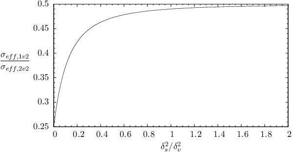
Therefore we see that there is a geometrical enhancement of the 2v1 contributions with respect to the 2v2 ones, and if the approximations (4) and (7) are valid, then this enhancement should be rather close to a factor of 2, as was first emphasised in Ref. [7].
The independent ladder pair and ladder splitting dPDFs, and , are calculated as follows.
Let us begin with the ladder splitting double PDF, and consider the case in which the scales are equal: . This is initiated at zero at some low scale :
| (12) |
is the scale at which perturbative splittings begin to occur, which should be of order of . The ladder splitting dPDF evolves according to the double DGLAP equation of Refs. [2, 4]:
| (13) |
In order to calculate the ladder splitting for (say), we start from the equal scale case and then evolve up in using the following evolution equation:
| (14) |
which only applies when . This equation is the equivalent of equation (9) in Ref. [41] (except there the evolution with respect to is presented when , so that equation differs from (14) by swapping the and indices). It is straightforward to show that equations (12), (13) and (14) are equivalent to equation (2.33) in Ref. [6].
To solve the differential equations (13) and (14) and obtain the ladder splitting dPDFs in practice we use the numerical code of Ref. [4]. A grid of dPDF values covering the ranges , was generated using 300 points in the direction, and 60 points in the direction for the evolution. We use the MSTW 2008 LO single PDFs [25] as the single PDFs in the evolution. Since the starting scale for these PDFs is GeV, we are not able to take lower than this value, and in fact we set GeV. We use the same and variable flavour number scheme as MSTW 2008 LO, with GeV and GeV.
For the independent pair distribution we must specify some nonperturbative input distributions at the input scale . Normally, due to the lack of information about the dPDFs, one commonly takes the input distributions to be a product of single PDFs:
| (15) |
Strictly speaking, this input should then be evolved up in scale using (13) with the final inhomogeneous term removed, and then (14) when . However, this evolution is almost equivalent to independent DGLAP evolution of the two partons, up to effects of the kinematic limit in the homogeneous double DGLAP evolution (which manifest themselves in equations (13) and (14) by the limits of the integrations being rather than ). This kinematic effect is known to be small unless is rather large [26], so if we take (15) as our input distributions, then to a good approximation, we can say:
| (16) |
Here we use (16) for the independent pair dPDFs. We take the single PDFs in this equation to be the MSTW 2008 LO PDFs for consistency with the ladder splitting dPDFs.
We should point out that in our study we ignore several effects. The first of these is crosstalk between the nonperturbatively generated ladder pair in the 2v1 graphs. This was first noticed in Ref. [6] but was also shown there to be numerically small in practice, so we can safely ignore it. We also ignore effects associated with correlations or interference in spin, colour, flavour, fermion number, and parton type between the two partons [27, 11]. Colour, fermion number and parton type correlations/interference are known to be Sudakov suppressed [28, 11, 8], but could potentially be non-negligible for small scales of order of a few GeV (see figure 10 of Ref. [8]). Spin correlations were studied in Ref. [26] in the context of the 2v2 process, and were found to be rather small after evolution, especially when both partons in were gluons. They were reduced to a few tens of per cent of the unpolarised contribution after only a few GeV of evolution, even in the most optimistic input scenario. However, it might be interesting to do a more detailed study of the spin effects, also including their effect in the 2v1 graphs. This is particularly in light of the experimentally observed azimuthal correlations between two mesons produced in proton-proton collisions [22], which cannot be described using an unpolarised DPS mechanism (either 2v2 or 2v1) [20, 21]. For the gluon-initiated processes we will discuss here, quark flavour interference is not a relevant effect since the flavour interference distributions are not able to mix with the double gluon distribution. Finally, we ignore interference between DPS and SPS, or twist 3 vs twist 3 terms, which were discussed in Refs. [11, 8]. It is possible to show that some of the twist 3 vs twist 3 effects are suppressed by helicity nonconservation in the associated diagrams [8, 29], but it seems likely that not all such effects are suppressed in this way – this topic needs further study.
In this paper we discuss production processes for which gluon-gluon fusion is the dominant process. We begin with processes in which a single particle is produced from the hard scattering process (). Then, at the leading order to which we work in this paper:
| (17) |
This allows us to simplify considerably the cross section. In this approximation one can easily get the cross section differential in rapidity of one and second object (meson or Higgs boson).
and
| (19) | |||||
This allows to easily calculate distributions in rapidity of and . In the last two equations the longitudinal momentum fractions are calculated from masses of the produced objects (quarkonia, Higgs bosons) and their rapidities
| (20) |
II.2 DPS production of
In Fig. 3 we show similar DPS mechanisms for production. The 2v1 mechanism (the second and third diagrams) were not considered so far in the literature.


In contrast to double quarkonium production in the case of production the cross section formula is a bit more complicated and the kinematical variables of each produced particle ( quark or antiquark) must be taken into account
| (21) | |||||
and
| (22) | |||||
for conventional and perturbative splitting contributions, respectively. The integration is 6-fold. The same is true for differential distributions. In the last two equations the longitudinal momentum fractions are calculated from the transverse masses of the produced quarks/antiquarks and their rapidities
| (23) |
The quantity corresponds to the transverse mass of either parton produced from the first hard subprocess, whilst corresponds to that from the second hard subprocess. The transverse mass is defined in the usual way to be .
II.3 Energy and process dependence of the effective cross section due to the presence of the perturbative splitting
The cross section for DPS production of some final states (e.g. , or ) can be written in a somewhat simplified way as:
| (24) |
and contain the functions and cross section of a process chosen11 1 In general above , and can be differential in ’s as well as can represent partially or fully phase space integrated quantities.. The equation is true both for phase space integrated cross section and differential distributions. The equation reflects the presence of the two components (2v2 and 2v1) as discussed above.
In phenomenology this is often simplified and written as
| (25) |
From the two equations above one gets:
| (26) |
If we assume that in addition one gets:
| (27) |
As will be discussed in this paper the ratio depends on the centre-of-mass energy and process considered. This means that as found from phenomenological analyses of the data (see Refs. [30, 31]) may depend on the energy as well as process considered. We shall discuss this in the Result section.
In early phenomenological estimates of that took into account only the 2v2 mechanism [43, 45], values of the order 30 mb were found. This is twice as large as the typical values found in the experimental studies ( 15 mb) [47, 48, 49, 50, 51, 52, 53]. In Ref. [17] it was argued that this discrepancy can be explained by the 2v1 mechanism. We also find a similar enhancement of the DPS cross section (i.e. reduction of ) by a factor of 2 coming from the 2v1 mechanism, as discussed below.
III Results
III.1 Double parton distributions
Before we present results for physical processes discussed in the present paper we wish to compare our independent ladder pair and ladder splitting dPDFs, and . In Fig. 4 we show plots of the dPDFs for selected parton combinations, and with factorization scale = 100 GeV2 (this is relevant for instance for meson production). The dPDFs shown are representative for all (49) combinations included in our full analysis.
One sees that the shapes of the dPDFs differ for the different parton combinations. Also, the overall size of the ladder splitting dPDFs are rather smaller than the independent ladder pair dPDFs – is typically of order at small . However, one notices that the shapes of the ladder splitting and independent ladder pair dPDFs are rather similar for fixed parton flavours , at least by eye. To get a better quantitative handle on this, we have plotted the ratios for each representative parton combination in Fig. 5. Indeed we see that the ratio takes a roughly constant value of for small . This is in accord with the plots of (or ) along the line given in Refs. [55, 54, 4] (although note that these plots were produced in the context of the old framework of Refs. [1, 2, 3]).
We believe that this similarity in shapes for small is related to the observation made in Refs. [6, 40] that for small the splitting in typically occurs extremely ‘early’ in (just above – e.g. less than 3 GeV for GeV even for rather large values of order [6]). Then, over most of the evolution range, the dominant evolution for the is the same as that for the (i.e. two parton branching evolution), and the similar evolution for and is what causes their shapes to converge. In order to test this idea we used the numerical code of Ref. [4] to calculate at GeV, taking various different forms for the input at GeV (a constant, , with or , etc.). For simplicity we set all the s to be the same – in practice the input is the important one determining the size of the s at low . We found very similar shapes in for GeV and regardless of the input distribution, which supports the idea that it is the evolution that causes the shapes to be similar. This qualitative behaviour is also found analytically in the double leading logarithmic approximation to the parton distributions [39], which is supposed to be valid in the limit . In this approximation one finds that the low behaviour is built up from the perturbative evolution, provided that the starting distribution is not too steep.
Another feature of note in the ratio plots is the large enhancement of the ratio when the fraction of the is close to , and the fraction of the is not too small – between and . The ratio is large here because the independent splitting dPDF is suppressed by the small size of the single PDF factor, whilst the perturbative splitting dPDF receives comparatively large contributions from direct splittings (the that splits then has to have a rather large , but the MSTW2008LO gluon density is quite large at = 100 GeV2 even at large ). As the fraction of the is decreased, the contribution from direct splittings to remains similar (since in this region it only depends on the much larger of the ), whilst the independent pair dPDF increases due to the PDF factor, and the ratio decreases. This explanation can be tested by plotting the ratio for the parton combination – then we expect no enhancement in the ratio of the kind that we found for the . This is because a gluon cannot directly split into a pair. We include the ratio as the final plot in Fig. 5, and indeed find that no enhancement of the ratio for this plot is found.
A further interesting point to make about the plot is that the ratio is roughly the same as the , or at small even though this distribution receives no direct feed from the inhomogeneous term in (13). This is due to the aforementioned point that for small final the splitting occurs very early, leaving plenty of evolution space for further emissions that allow (for example) a to eventually give rise to a pair (plus various other emitted partons). This means that we cannot suppress the 2v1 contribution to DPS by picking processes such as same sign that are initiated by such parton pairs (unless one finds a way to probe very large s in this process).
The similar shape of the ladder splitting dPDFs for small as compared to the independent ladder dPDFs indicates that the differential cross section contributions associated with the 2v1 and 2v2 mechanisms will be rather similar. This we will see in the next two subsections.


III.2 Quarkonium production
In the calculations, results of which will be discussed below, we assume , where is a generic name for the S-wave, P-wave quarkonium or Higgs boson mass.
In Table 2 we present the ratio of for the production of two identical-mass objects (two identical quarkonia, two Higgs bosons). Following our earlier discussion from section II.1 we take the ratio . The ratio only slightly depends on the mass of the object and centre-of-mass energy but the tendency is rather clear. The masses chosen correspond roughly to production of , (M = 3 GeV), , (M = 10 GeV) quarkonia and Higgs boson (M = 126 GeV). The double Higgs case is purely academic as the corresponding DPS cross section is rather small (a 10-4 fraction of fb, much smaller than the single parton scattering cross section [33, 34, 35, 36, 37]) but the effect of the perturbative splitting can be here well illustrated.
| M (GeV) / (TeV) | 0.2 | 0.5 | 1.96 | 8.0 | 13.0 |
| 3. | 0.840 | 0.775 | 0.667 | 0.507 | 0.437 |
| 10. | 1.116 | 1.022 | 0.891 | 0.780 | 0.743 |
| 126. | – | — | 1.347 | 1.134 | 1.070 |
In Fig. 6 we show the ratio defined as
| (28) |
From these plots we can see that does not depend strongly on the rapidities and , as one would expect given that the ratio of the ladder splitting and independent ladder pair dPDFs does not depend strongly on (Fig. 5).


In the calculation of the cross sections in this and in the next subsection we have to fix the two nonperturbative parameters: and . Their values are not well known. Once again we take the ratio . We choose = 30 mb which corresponds to assuming that partons in a ‘nonperturbatively generated’ pair are essentially uncorrelated in transverse space [43, 45] (but note that varying with the ratio fixed affects only the normalisations of the cross sections presented below).
In Fig. 7 we show how the empirical value depends on centre-of-mass energy assuming that the value of is independent of energy. We see a clear dependence of on energy in the plot, and also on the mass of the quarkonium. Assuming that there is no other mechanism for an energy dependence of , is therefore expected to increase with centre-of-mass energy. Note also that the empirical value obtained is in the ball park of the values extracted in experimental measurements of DPS ( mb), even though is rather larger, assumed here to be 30 mb.

III.3 production
Now we proceed to double charm production. Here we either assume and , or and . The quantity is the transverse mass of either parton emerging from subprocess , whilst is the invariant mass of the pair emerging from subprocess . In Table 3 we show the ratio of 2v1-to-2v2 cross sections for different centre of mass energies. The numbers here are similar to those for the double quarkonium production.
| (GeV2) / (TeV) | 0.2 | 0.5 | 1.96 | 7.0 | 13.0 |
| 0.628 | 0.610 | 0.503 | 0.326 | 0.254 | |
| 0.914 | 0.855 | 0.760 | 0.667 | 0.606 |
Let us show now some examples of differential distributions. In Fig. 8 we show the rapidity distribution of the charm quark/antiquark for different choices of the scale at = 7 TeV. The conventional and splitting terms are shown separately. The splitting contribution (lowest curve, red online) is smaller, but has almost the same shape as the conventional DPS contribution. We wish to note the huge difference arising from the different choices of factorization scale. The second choice leads to cross sections more adequate for the description of the LHCb data for double same-flavor meson production [22].


In Fig. 9 we show corresponding distributions in transverse momentum of charm quark/antiquark. Again the shapes of conventional and splitting contributions are almost the same.


The corresponding ratios of the 2v1-to-2v2 contributions as a function of rapidity (left) and transverse momentum (right) are shown in Fig. 10. Especially the transverse momentum dependence shows a weak but clear tendency.


Finally in Fig. 11 we show the empirical , this time for double charm production. Again rises with the centre-of-mass energy. A rather large difference between different choices of scales can be observed.

IV Conclusion
In the present paper we have presented first quantitative estimates of the single perturbative splitting 2v1 contribution to double quarkonium, double Higgs boson and production. In all cases we find that the splitting contribution is of the same order of magnitude as the more conventional 2v2 contribution often discussed in the literature. This is consistent with the observation made already in Ref. [17]. The perturbative splitting contribution was not considered explicitly in previous detailed analyses of and pairs of the same-flavor mesons.
Our calculation shows that the parton-splitting contribution is not negligible and has to be included in the full analysis. However, it is too early in the moment for detailed predictions of the corresponding contributions as our results strongly depend on the values of not well known parameters and . Both their magnitude and even their ratio are not well known. We have presented only some examples inspired by a simple geometrical model. A better understanding of the two nonperturbative parameters seems an important future task.
We have shown that almost all differential distributions (in rapidity, transverse momentum, even many two-dimensional distributions) for the conventional and the parton-splitting contributions have essentially the same shape. This makes their model-independent separation extremely difficult. This also shows why the analyses performed so far could describe different experimental data sets in terms of the conventional 2v2 contribution alone. The sum of the 2v1 and 2v2 contributions behaves almost exactly like the 2v2 contribution, albeit with a smaller that depends only rather weakly on energy, scale and momentum fractions.
With the perturbative 2v1 mechanism included, increases as is increased, and decreases as is increased. A decrease of with was also observed in Ref. [7] for the same reason. Similar trends were also observed in Ref. [32], although the calculation there is performed in a BFKL framework rather than the DGLAP framework used here. In Ref. [32] the decrease of the effective with is somewhat stronger. It is difficult to pin down the exact reason for this difference due to the different calculational frameworks used. However, we remark that the definitions of the 2pGPDs and total DPS cross section used in Ref. [32] would, in the DGLAP framework, allow some effective 1v1 contribution to DPS, which here we do not include.
At present only the leading-order version of the single perturbative splitting formalism is available. However, it is well known that NLO corrections for the gluon initiated processes are rather large, also for processes considered here. In the case of production they can be taken into account e.g. in the -factorization [38]. It is not clear in the moment how to combine the higher-order effects with the perturbative splitting mechanism discussed here. An interesting question is whether the ratio between the 2v1 and 2v2 contributions changes when higher-order corrections are included. Further studies are clearly needed.
Acknowledgments
One of us (A.S) is indebted to Alexander Snigirev for a discussion and interesting comments. We thank Markus Diehl for various useful comments on the manuscript. This work was partially supported by the Polish NCN grant DEC-2011/01/B/ST2/04535 as well as by the Centre for Innovation and Transfer of Natural Sciences and Engineering Knowledge in Rzeszów.
References
- [1] R. Kirschner, Phys. Lett. B84 (1979) 266.
- [2]
V. P. Shelest, A. M. Snigirev and G. M. Zinovjov,
Phys. Lett. B113 (1982) 325;
G. Zinovev, A. Snigirev and V. Shelest, Theor. Math. Phys. 51 (1982) 523. - [3] A. M. Snigirev, Phys. Rev. D68 (2003) 114012.
- [4] J. R. Gaunt and W. J. Stirling, JHEP 1003 (2010) 005.
- [5] J. R. Gaunt and W. J. Stirling, JHEP 1106, 048 (2011) [arXiv:1103.1888 [hep-ph]].
- [6] J. R. Gaunt, J. High Energy Phys. 01 (2013) 042; arXiv:1207.0480 [hep-ph].
- [7] B. Blok, Yu. Dokshitser, L. Frankfurt and M. Strikman, Eur. Phys. J. C 72, 1963 (2012) [arXiv:1106.5533 [hep-ph]].
- [8] A. V. Manohar and W. J. Waalewijn, Phys. Rev. D 85, 114009 (2012) [arXiv:1202.3794 [hep-ph]].
- [9] A. V. Manohar and W. J. Waalewijn, Phys. Lett. B 713, 196 (2012) [arXiv:1202.5034 [hep-ph]].
- [10] M. Diehl and A. Schäfer, Phys. Lett. B698 (2011) 389.
- [11] M. Diehl, D. Ostermeier and A. Schäfer, JHEP 03 (2012) 089.
- [12] M.G. Ryskin and A.M. Snigirev, Phys. Rev. D83 (2011) 114047.
- [13] E. Cattaruzza, A. Del Fabbro and D. Treleani, Phys. Rev. D 70, 034022 (2004) [hep-ph/0404177].
- [14] M. Strikman and D. Treleani, Phys. Rev. Lett. 88, 031801 (2002) [hep-ph/0111468].
- [15] H. D. Politzer, Nucl. Phys. B 172, 349 (1980).
- [16] N. Paver and D. Treleani, Nuovo Cim. A 70, 215 (1982).
- [17] B. Blok, Yu. Dokshitzer, L. Frankfurt and M. Strikman, arXiv:1306.3763.
- [18] M. Cacciari, G. P. Salam and S. Sapeta, JHEP 1004, 065 (2010) [arXiv:0912.4926 [hep-ph]].
- [19] M. Łuszczak, R. Maciuła and A. Szczurek, Phys. Rev. D85 (2012) 094034; arXiv:1111.3255 [hep-ph].
- [20] R. Maciuła and A. Szczurek, Phys. Rev. D87 (2013) 074039; arXiv:1301.4469 [hep-ph].
- [21] A. van Hameren, R. Maciula and A. Szczurek, Phys. Rev. D89 (2014) 094019; arXiv:1402.6972 [hep-ph].
- [22]
R. Aaij et al. (LHCb Collaboration),
J. High Energy Phys. 06, 141 (2012);
arXiv:1205.0975 [hep-ex]. - [23] W. Schäfer and A. Szczurek, Phys. Rev. D85 (2012) 094029; arXiv:1203.4129 [hep-ph].
- [24] B. Blok, Yu. Dokshitzer, L. Frankfurt and M. Strikman, Phys. Rev. D 83, 071501 (2011) [arXiv:1009.2714 [hep-ph]].
- [25] A. D. Martin, W. J. Stirling, R. S. Thorne and G. Watt, Eur. Phys. J. C 63, 189 (2009) [arXiv:0901.0002 [hep-ph]].
- [26] M. Diehl, T. Kasemets and S. Keane, JHEP 1405, 118 (2014) [arXiv:1401.1233 [hep-ph]].
- [27] M. Mekhfi, Phys. Rev. D 32, 2380 (1985).
- [28] M. Mekhfi and X. Artru, Phys. Rev. D 37, 2618 (1988).
- [29] J. -W. Qiu and G. F. Sterman, Nucl. Phys. B 353, 105 (1991).
- [30] M. H. Seymour, and A. Siódmok, J. High Energy Phys. 10, 113 (2013); arXiv:1307.5015 [hep-ph].
- [31] M. Bähr, M. Myska, M. H. Seymour and A. Siódmok, J. High Energy Phys. 03, 129 (2013); arXiv:1302.4325 [hep-ph].
- [32] C. Flensburg, G. Gustafson, L. Lönnblad and A. Ster, J. High Energy Phys. 06, 066 (2011).
- [33] T. Plehn, M. Spira and P. M. Zerwas, Nucl. Phys. B 479, 46 (1996) [Erratum-ibid. B 531, 655 (1998)] [hep-ph/9603205].
- [34] S. Dawson, S. Dittmaier and M. Spira, Phys. Rev. D 58, 115012 (1998) [hep-ph/9805244].
- [35] T. Binoth, S. Karg, N. Kauer and R. Ruckl, Phys. Rev. D 74, 113008 (2006) [hep-ph/0608057].
- [36] J. Baglio, A. Djouadi, R. Gröber, M. M. Mühlleitner, J. Quevillon and M. Spira, JHEP 1304, 151 (2013) [arXiv:1212.5581 [hep-ph]].
- [37] R. Frederix, S. Frixione, V. Hirschi, F. Maltoni, O. Mattelaer, P. Torrielli, E. Vryonidou and M. Zaro, Phys. Lett. B 732, 142 (2014) [arXiv:1401.7340 [hep-ph]].
- [38] R. Maciuła and A. Szczurek, Phys. Rev. D87 (2013) 094022; arXiv:1301.3033 [hep-ph].
- [39] R. K. Ellis, W. J. Stirling and B. R. Webber, “QCD and collider physics,” Camb. Monogr. Part. Phys. Nucl. Phys. Cosmol. 8, 1 (1996).
- [40] M.G. Ryskin and A.M. Snigirev, Phys. Rev. D86 (2012) 014018.
- [41] F. A. Ceccopieri, Phys. Lett. B 697, 482 (2011) [arXiv:1011.6586 [hep-ph]].
- [42] S. Domdey, H. -J. Pirner and U. A. Wiedemann, Eur. Phys. J. C 65, 153 (2010) [arXiv:0906.4335 [hep-ph]].
- [43] L. Frankfurt, M. Strikman and C. Weiss, Phys. Rev. D 69 (2004) 114010 [hep-ph/0311231].
- [44] I. Bender, H. G. Dosch, H. J. Pirner and H. G. Kruse, Nucl. Phys. A 414, 359 (1984).
- [45] G. Calucci and D. Treleani, Phys. Rev. D 60, 054023 (1999) [hep-ph/9902479].
- [46] B. Povh, Nucl. Phys. A 699, 226 (2002).
- [47] Axial Field Spectrometer Collaboration, T. Akesson et al., Z.Phys. C34, 163 (1987).
- [48] CDF Collaboration, F. Abe et al., Phys.Rev.Lett. 79, 584 (1997).
- [49] CDF Collaboration, F. Abe et al., Phys.Rev. D56, 3811 (1997).
- [50] D0 Collaboration, V. Abazov et al., Phys.Rev. D81, 052012 (2010), [0912.5104].
- [51] ATLAS Collaboration, G. Aad et al., New J.Phys. 15, 033038 (2013), [1301.6872].
- [52] CMS Collaboration, S. Chatrchyan et al., JHEP 1403, 032 (2014), [1312.5729].
- [53] ATLAS Collaboration, G. Aad et al., JHEP 1404, 172 (2014), [1401.2831].
- [54] E. Cattaruzza, A. Del Fabbro and D. Treleani, Phys. Rev. D 72, 034022 (2005) [hep-ph/0507052].
- [55] V. L. Korotkikh and A. M. Snigirev, Phys. Lett. B 594 (2004) 171 [hep-ph/0404155].