Actions of mapping class groups

In this subsection, we consider the action of the mapping class group on Thurston’s sphere $\mathcal{PMF}$ of projective equivalence classes of measured foliations of a surface. This space carries a natural projective piecewise-linear structure. The union of Teichmüller space with this sphere is a beautiful example of a compact space homeomorphic to a closed ball whose interior carries a natural smooth structure (in fact, it carries a natural complex-analytic structure) and whose boundary carries a natural projective piecewise-linear structure which is far from being smooth. It was constructed by Thurston as a natural compactification of Teichmüller space, and it plays a fundamental role in the proof he gave of his classification theorem of mapping classes.

We shall recall the basic elements of Thurston’s piecewise-linear (PL) structure of $\mathcal{MF}$ defined by train tracks and the quotient projective piecewise-linear (PPL) structure of $\mathcal{PMF}$.

We note right away that the PL atlas defined by train tracks is not a maximal atlas in the sense of analytic structures; in fact, one can easily see that if we take the maximal atlas associated to this PL structure, we get a PL structure whose automorphism group is uncountable, and therefore it cannot be the mapping class group.

We first recall the definition of measured foliations and of the space $\mathcal{MF}$.

We consider foliations on $S$ with singular points which are of the type given in Figure 1. For singular points on the boundary, the local model is such that if we double the surface along its boundary components, we get allowable singularities (as interior singular points). Examples of singular points at the boundary are represented in Figure 2.

A transverse measure for a foliation is a measure on each transverse arc which is equivalent to the Lebesgue measure of a compact interval of $\mathbb{R}$ such that these measures are invariant by the local holonomy maps, that is, the isotopies of arcs that keep each point on the same leaf.

A Whitehead move between two measured foliations is the operation of contracting to a point a compact leaf that joins two singular points, or the inverse operation. The move is well-defined up to an ambient isotopy. An example of a Whitehead move is represented in Figure 3.

The equivalence relation between measured foliations is generated by ambient isotopy and Whitehead moves that preserve transverse measure.

Given a measured foliations $F$ on $S$, we shall use the notation $[F]$ for its equivalence class in $\mathcal{MF}$, and sometimes also $F$ (without the brackets) when no confusion is possible.

The space of equivalence classes of measured foliations is called measured foliation space, and it is denoted by $\mathcal{MF}$ or $\mathcal{MF}(S)$. It is equipped with a topology which is defined via its embedding in the space $\mathbb{R}^{\mathcal{S}}_{+}$ of nonnegative functions on the set $\mathcal{S}$ of isotopy classes of essential simple closed curves on $S$. This is done using the geometric intersection function which we recall now.

Given a measured foliation $F$ on $S$ and an element $\gamma$ in $\mathcal{S}$, $i(F,\gamma)$ is the infimum of the total measure of $c$ over all closed curves $c$ in the homotopy class $\gamma$ which are concatenations of arcs transverse to $F$ and arcs contained in the leaves of $F$. The total measure of $c$ is the sum of the measures of the subarcs transverse to $F$.

The value $i(F,\gamma)$ does not depend on the choice of the equivalence class of $F$. We obtain in this way a map

called the geometric intersection function, or, in short, intersection function.

Using this function, we obtain a natural map

from $\mathcal{MF}$ to $\mathbb{R}_{+}^{\mathcal{S}}$. This map is injective, and $\mathcal{MF}$ inherits a topology from this injection, the space $\mathbb{R}_{+}^{\mathcal{S}}$ being equipped with the product topology. Equipped with this topology, $\mathcal{MF}$ is homeomorphic to $\mathbb{R}^{6g-6}\setminus\{0\}$. All these results are due to Thurston [163] and they are proved in [46]. It is sometimes practical to consider the empty foliation as an element of $\mathcal{MF}$ and in this case the space becomes homomorphic to $\mathbb{R}^{6g-6}$.

There is a natural action of the group of positive reals $\mathbb{R}_{+}^{*}$ on $\mathcal{MF}$ obtained from the action of $\mathbb{R}_{+}^{*}$ on measured foliations defined by multiplying the transverse measure by a constant positive factor. The quotient space of $\mathcal{MF}$ by this action is the projective foliation space, denoted by $\mathcal{PMF}$.

From the embedding of $\mathcal{MF}$ into the space $\mathbb{R}_{+}^{\mathcal{S}}$ we obtain an embedding of $\mathcal{PMF}$ in the projective space $\mathbb{P}\mathbb{R}_{+}^{\mathcal{S}}$.

It will be convenient in this subsection and in the next one to represent an element of $\mathcal{MF}$ by a partial measured foliation. This is a measured foliation whose support, $\mathrm{Supp}(F)$, is a nonempty (and not necessarily connected) subsurface $S^{\prime}$ with boundary of $S$ such that the boundary curves of $S^{\prime}$ are all essential in $S$. The partial foliation may have singularities at the boundary of $S^{\prime}$, but in the complement of these singular points the foliation is tangent to the boundary of $S^{\prime}$. Any partial measured foliation on $S$ gives a well-defined element of $\mathcal{MF}$, which is the equivalence class of the measured foliation obtained by collapsing each non-foliated region onto a spine, cf. [46].

We now recall the theory of train tracks which is at the basis of the piecewise-linear theory of $\mathcal{MF}$.

A train track $\tau$ on $S$ is a graph embedded in $S$ whose vertices we shall suppose trivalent (although this is not necessary) and such that at any vertex, the three half-edges that abut have a well-defined tangent at that point; that is, we have a notion of two half-edges abutting from one side and of the remaining half-edge abutting from the other side. (In fact, the use of the word “tangent” here can be somehow misleading, since no smooth structure on $S$ is needed in the theory. Instead, one can simply say that there is a well-defined notion of “two half-edges abutting from one side” and “one half-edge abutting from the other side” at each vertex. Equivalently, we just single out one of the three half-edges abutting at each vertex.)

The local structure at a vertex is represented in Figure 4.

A vertex of $\tau$ is also called a switch. We shall call a corner of $S$ a region in a neighborhood of a switch which is contained between the two half-edges that abut from the same side.

An edge of a train track is a connected component of the complement of the set of switches. We note that a train track may have no vertices at all, i.e. it could consist of a union of disjoint simple closed curves; in that case we shall also call such a closed curve an edge of the train track.

On a surface with boundary, a train track may be either tangent or transverse to the boundary.

On closed surfaces, all the train tracks $\tau$ that we consider satisfy the following condition: no connected component of $S\setminus\tau$ is a disc with $0$, $1$ or $2$ corners or an annulus with no corner (see Figure 5). We shall call such a train track admissible whenever this property needs to be referred to (although all our train tracks will be admissible).

For surfaces with boundary, the excluded complementary components are those such that they give rise to excluded complementary components on the closed surfaces obtained by doubling the surfaces with boundary.

Train track theory works for general surfaces of finite type, with punctures and/or boundary components, but in order to avoid several technicalities, we shall deal from now on with the case where $S$ is a closed surface.

A train track $\tau$ is said to be maximal if every component of $S\setminus\tau$ is a disc with three corners on its boundary.

There are three basic moves that can be performed on a train track and they are represented in Figure 6. They are called a shift, a right split and a left split. These three moves will be essential in what follows.

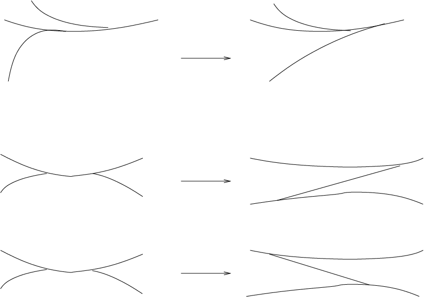
Any train track $\tau$ has a regular neighborhood $N(\tau)$ foliated by arcs that are called the ties. The local picture of the foliation by the ties near a switch is represented in Figure 7. The regular neighborhood $N(\tau)$, equipped with its foliation by the ties, is well-defined up to isotopy, and there is a natural projection $N(\tau)\searrow\tau$ from $N(\tau)$ to a train track (isotopic to) $\tau$ defined by collapsing each tie to a point.

Let $\tau$ be a train track on $S$ and let $e_{1},\ldots,e_{N}$ be its edges. Let $\mathbb{R}^{N}$ denote the real vector space with basis $\{e_{1},\ldots,e_{N}\}$ and let $(x_{1},\ldots,x_{N})$ denote the coordinates of a point in that space. We let $V_{\tau}\subset\mathbb{R}^{N}$ be the closed convex cone in $\mathbb{R}^{N}$ defined by the system of equations

where, in the last equation, $x_{j}$ and $x_{k}$ denote the coordinates at the two edges that abut from the same side at the given switch, and $x_{i}$ the coordinate on the edge that abuts from the other side.

The coordinates $x_{i}$ on the edges are also called the weights of the edge.

A train track $\tau$ is said to be recurrent if there exists an element $(x_{1},\ldots,x_{N})$ of $V_{\tau}$ satisfying $x_{i}>0$ for all $i=1,\ldots,N$.

For any train track $\tau$ on $S$, there is a map

defined as follows:

Consider the regular neighborhood $N(\tau)$ of $\tau$ equipped with its projection $N(\tau)\searrow\tau$ and let $(x_{1},\ldots,x_{N})$ be a nonzero element of $V_{\tau}$. For each nonzero coordinate $x_{i}$ ($i\in\{1,\ldots,N\}$), consider the inverse image of the edge $e_{i}$ by the projection $N(\tau)\searrow\tau$. The closure of the interior of this inverse image has a natural structure of a rectangle equipped with a foliation induced by the ties, which we call the vertical foliation. We equip this rectangle with another foliation, which we call the horizontal foliation, whose leaves are segments which are transverse to the ties and which join the two vertical edges of the rectangle, that is, the two edges that consist of ties. We equip this horizontal foliation with a transverse measure whose total mass is equal to $x_{i}$.

Finally, we glue the various foliated rectangles so obtained along their vertical sides, by using measure-preserving homeomorphisms. We obtain a partial measured foliation on $S$, which gives a well-defined element of $\mathcal{MF}$. The zero element of $V_{\tau}$ is sent to the empty foliation of $\mathcal{MF}$. This defines the map $\varphi_{\tau}:V_{\tau}\to\mathcal{MF}$.

The notion of train track was introduced by Thurston in [162]. A standard reference on train tracks is the monograph [146] by Penner and Harer. The following result is outlined by Thurston in his Notes [162]. A proof is contained in [132] p. 20 and ff.

A measured foliation $F$ (or its equivalence class $[F]\in\mathcal{MF}$) is said to be carried by a train track $\tau$ if $[F]$ is in the image set of $V_{\tau}$ by the map $\varphi_{\tau}$ in (1).

We need to recall the definition of a PL map.

Let $M$ be a positive integer. A (closed) linear half-space in $\mathbb{R}^{M}$ is (the closure of) a connected component of the complement of a hyperplane. We shall say that a subset $V$ of $\mathbb{R}^{M}$ is a linear polytope if it is the intersection of a finite number of closed linear half-spaces of $\mathbb{R}^{M}$. Let us stress on the fact that we are talking about linear and not only affine half-spaces, so that a linear polytope $V$ is $\mathbb{R}_{+}^{*}$-homogeneous (invariant by multiplication by elements of $\mathbb{R}_{+}^{*}$). In particular, it is noncompact (unless it is empty). All the polytopes we consider are linear. With this in mind, we shall henceforth use the name polytope to denote a linear polytope.

The dimension of a polytope $V\subset\mathbb{R}^{M}$ is the dimension of the smallest (in the sense of inclusion) linear subspace of $\mathbb{R}^{M}$ that contains it. It is also the smallest dimension of a vector space in which $V$ embeds.

Note that a polytope is closed and convex.

The relative interior of a polytope $V$ is the topological interior of $V\cap A$ in $A$, with $A$ being the smallest linear subspace of $\mathbb{R}^{M}$ containing $V$.

Let $M$ and $N$ be two positive integers, let $V\subset\mathbb{R}^{M}$ be a finite union of polytopes of the same dimension, $V_{1},\ldots,V_{n}\subset\mathbb{R}^{M}$, and let $f:V\to\mathbb{R}^{N}$ be a map. We shall say that $f$ is PL relative to the decomposition $V=V_{1}\cup\ldots\cup V_{n}$ if $f$ is continuous and if the restriction of $f$ to the relative interior of each of the polytopes $V_{1},\ldots,V_{n}$ is the restriction of a linear map from $\mathbb{R}^{M}$ to $\mathbb{R}^{N}$.

Given a subset $V$ of $\mathbb{R}^{M}$, we shall say that a map $f:V\to\mathbb{R}^{N}$ is piecewise-linear (PL) if it is PL relatively to some decomposition of $V$ as a union of polytopes $V_{1},\ldots,V_{n}$.

For each maximal recurrent train track $\tau$, we let $U_{\tau}=\varphi_{\tau}(V_{\tau})\subset\mathcal{MF}$ be the image of the associated map $\varphi_{\tau}:V_{\tau}\to\mathcal{MF}$ and we let $\psi_{\tau}:U_{\tau}\to V_{\tau}$ denote the inverse of the homeomorphism $\varphi_{\tau}:V_{\tau}\to\varphi(V_{\tau})=U_{\tau}$ of Theorem 3.1.

Let $\mathcal{A}$ be the following collection of maps:

The meaning of this statement is that the coordinate changes of this atlas are PL.

We shall prove a rigidity theorem (Theorem 3.11 below) for the automorphism group of this structure, which we call the train track PL structure of $\mathcal{MF}$. The proof of this theorem uses a precise description of the coordinate changes $\psi_{\tau^{-1}\sigma}=\psi_{\sigma}\circ\psi_{\tau}^{-1}$ of the atlas $\mathcal{A}$, each such coordinate change map being defined on an appropriate subset of $V_{\tau}$. We shall recall here some details given in Chapter 1 of [132], because we shall use them in the proof of Theorem 3.11.

If $\tau$ and $\sigma$ are two train tracks on $S$, we say that $\tau$ is carriedby $\sigma$, and we write this relation as $\tau\prec\sigma$, if $\tau$ is isotopic to a train track $\tau^{\prime}$ which is contained in a regular neighborhood $N(\sigma)$ of $\sigma$ and which is transverse to the ties of $N(\sigma)$. When $\tau\prec\sigma$, there is a natural linear map from the closed convex cone $V_{\tau}$ to the closed convex cone $V_{\sigma}$ which induces the inclusion map at the level of the two subspaces $\varphi_{\tau}(V_{\tau})$ and $\varphi_{\sigma}(V_{\sigma})$ of $\mathcal{MF}$. The map $V_{\tau}\to V_{\sigma}$ is defined by associating to each weight system on the edges of $\tau$ the weigh system on the edges of $\sigma$ where the weight on an edge $e$ is defined as the sum of the edges of $\tau$ (counted with multiplicity) that traverse a tie which is an inverse image of $e$ with respect to the map $N(\tau)\searrow\tau$. (The result is independent of the choice of the tie).

The following definition and proposition are needed in the proof of Theorem 3.11.

Property (3) of Proposition 3.4 implies that the restriction of the coordinate change map $\psi_{\tau^{-1}\sigma}$ to the neighborhood $N(F)$ of $F$ is linear on each subset $U_{\tau_{i}}$ of $N(F)$. In fact, $\psi_{\tau^{-1}\sigma}$ is PL relative to the given decomposition.

Proposition 3.4 is the basic technical result which implies that the coordinate changes in the atlas $\mathcal{A}$ are piecewise-linear. Without going deeply into the details, let us give an idea of the proof. Full details are given in [132], Chapter 1.

The proof of the rigidity theorem is based on an analysis of the structure of the set of singular points of the train track PL functions, that is, the points where $f$ is not linear. Indeed, in the atlas $\mathcal{A}$, there are points where non-linearity occurs, and points where non-linearity cannot occur. There is also a hierarchy on the set of points where non-linearity may occur: there are points where it may be more severe than at others. Let us give right away the reason for that. The change of coordinates, for the PL atlas, are obtained by repeated application of the elementary moves on the train tracks (shifts and splits). These elementary moves define subdivisions of the domains of the charts in $\mathcal{A}$ that parametrize the measured foliations classes. At the level of foliations carried by the train track, an elementary move is performed when the foliation has compact leaves joining singular points. Thus the “bad sets” of the PL structure (that is, those where the coordinate change is not linear) are classes of measured foliations which have compact leaves joining singular points. And the more there are such compact leaves, the more one can perform subdivisions of the domain of the chart, that is, the larger can be the codimension of the singular set to which this point belongs. By examining the topology of measured foliations, we see that the highest degree of singularity corresponds to the set of equivalence classes of measured foliations that are represented by simple closed curves. Thus, this subset of $PMF$ is preserved by a PL map. For similar reasons, the subset of measured foliations represented by systems of $n$ simple closed curves with $n$ fixed is also preserved. This gives the induced action of a PL homeomorphism of $\mathcal{MF}$ (or $\mathcal{PMF}$) on the curve complex.

Now we give some more definitions which make these ideas more precise.

We observe the following two facts:

(F1) The set $\mathrm{Sing}(f)$ is a union of codimension-1 submanifolds of $V$, each of which is equal to the intersection of two sets in the collection of polytopes $\{V_{1},\ldots,V_{n}\}$.

(F2) If the polytopes $V_{i}$ have dimension $D$, then $\mathrm{Sing}(f)$ is contained in a union of polytopes of dimension $D-1$ in $\mathbb{R}^{M}$ such that the restriction of $f$ to $\mathrm{Sing}(f)$ is PL.

Repeating this, we find a nested sequence of subsets of $V$,

where:

1. (1)

   $\mathrm{Sing}_{0}(f)=\mathrm{Sing}(f)$;

2. (2)

   for every integer $i$ satisfying $2\leq i\leq k$, $\mathrm{Sing}_{i}(f)$ is the singular set of the restriction of $f$ to $\mathrm{Sing}_{i-1}(f)$.

Note that $k\leq n$ and that for each $2\leq i\leq k$, $\mathrm{Sing}_{i}(f)$ is contained in a codimension-1 subset of $\mathrm{Sing}_{i-1}(f)$ (see Observation (F2) above).

Let $f$ be a PL function defined on a set $V=V_{1}\cup\ldots\cup V_{n}$ as above. The associated sequence $\mathrm{Sing}_{0}(f)\supset\mathrm{Sing}_{1}(f)\supset\ldots\mathrm{Sing}_{k}(f)$ defines a stratification of $V$, each stratum having a well-defined codimension in $V$. We shall call this stratification the flag induced by $f$ on the set $V$, and we shall denote this flag equipped by its stratification by $\mathrm{Fl}(f)$.

Now we consider more precisely the PL functions relative to the train track PL structure.

Let $\mathcal{P}$ be the set of train track PL functions on $\mathcal{MF}$. Due to the last condition in Definition 3.6, the set $\mathcal{P}$ is the set of smoothest possible maps on $\mathcal{MF}$ relatively to the atlas $\mathcal{A}$.

The homeomorphisms of $\mathcal{PMF}$ that preserve the train track PL structure form a group, which we call the automorphism group of the train track PL structure. We denote this group by $\mathrm{Aut}(\mathcal{PMF},\mathcal{P})$.

From Proposition 3.8, we get a homomorphism

Our next goal is to prove that, except for a finite number of special surfaces (like in most of the other rigidity theorems), this homomorphism is an isomorphism (Theorem 3.11 below).

Before proving this theorem, we need to establish a few more notation and results.

A system of curves on $S$ is the isotopy class of a collection of disjoint and pairwise non-isotopic essential curves on $S$. For $g\geq 2$, the number of elements in such a collection is bounded above by $3g-3$.

For each $k$ satisfying $1\leq k\leq 3g-3$, let $\mathcal{MF}_{k}\subset\mathcal{MF}$ be the set of measured foliation classes $x$ satisfying the following:

1. (1)

   There is no chart $(U_{\tau},\psi_{\tau})$ in $\mathcal{A}$ having $x$ in the interior of its domain $U_{\tau}$ such that there exists a coordinate change $\psi_{\tau^{-1}\sigma}$ having $\psi_{\tau}(x)$ in the interior of its domain, with $\psi_{\tau}(x)$ being on a stratum of dimension $\leq k-1$ of the flag $\mathrm{Fl}(\psi_{\tau\sigma})$.

2. (2)

   There exists a coordinate chart $(U_{\tau},\psi_{\tau})$ in $\mathcal{A}$ having $x$ in the interior of its domain and a coordinate change $\psi_{\tau^{-1}\sigma}$ having $\psi_{\tau}(x)$ in the interior of its domain, such that $\psi_{\tau}(x)$ is on a stratum of dimension $k$ of the flag $\mathrm{Fl}(\psi_{\tau^{-1}\sigma})$.

3. (3)

   The element $\psi_{\tau}(x)$ is a convex combination of $k$ elements in the 1-stratum of $\mathrm{Fl}(\psi_{\tau^{-1}\sigma})$ with respect to the linear structure on $V_{\tau}=\psi_{\tau}(U_{\tau})$ induced from its inclusion in $\mathbb{R}^{N}$.

In particular, $\mathcal{MF}_{1}\subset\mathcal{MF}$ is simply the set of measured foliation classes $x$ such that there exists a coordinate chart $(U_{\tau},\psi_{\tau})$ in $\mathcal{A}$ having $x$ in the interior of its domain and a coordinate change $\psi_{\tau^{-1}\psi}$ having $\psi_{\tau}(x)$ in the interior of its domain such that $x$ is on a stratum of dimension 1 of the flag $\mathrm{Fl}(\psi_{\tau^{-1}\sigma})$ defined by the singular set of the coordinate change.

The proof of the rigidity theorem 3.11 is based on a geometric characterization of the elements in each set $\mathcal{MF}_{k}$, which we give now.

Let $\mathcal{S^{\prime}}$ be the set of homotopy classes of systems of curves on $S$, that is, the set of homotopy classes of unions of disjoint pairwise non-homotopic simple closed curves.

We assume that $g\geq 2$ and, for every integer $k$ satisfying $1\leq k\leq 3g-3$, we denote by $\mathcal{S}_{k}$ the subset of $\mathcal{S}^{\prime}$ consisting of isotopy classes of systems of curves of cardinality $k$.

In particular $\mathcal{S}_{1}=\mathcal{S}$.

Recall that for each integer $k$ satisfying $1\leq k\leq 3g-3$, there is a natural inclusion $j_{k}:(\mathbb{R}_{+}^{*})^{k}\times\mathcal{S}_{k}\hookrightarrow\mathcal{MF}$, defined by associating to each $v\in(\mathbb{R}_{+}^{*})^{k}$ and to each element $C\in\mathcal{S}_{k}$ the equivalence class of a partial measured foliation $F$ which has the following properties:

1. (1)

   The support of $F$ is the union of disjoint annuli $A_{1},\ldots,A_{k}$ which are foliated by closed leaves;

2. (2)

   each annulus $A_{i}$ is a regular neighborhood of a closed curve $c_{i}$, where $c_{1},\ldots,c_{k}$ are the components of a system of curves representing the isotopy class $C$;

3. (3)

   for $1\leq i\leq k$, the total transverse measure of the annulus $A_{i}$ is equal to the $i$-th coordinate of $v$.

We shall call a foliation on $S$ representing an element of $\mathcal{MF}$ which is the image of some element of $\mathcal{S}^{\prime}$ by one of the maps $j_{k}$ an annular foliation.

The rigidity result, Theorem 3.11, can be seen as a rigidity theorem for some boundary structure of Teichmüller space. We mention the following:

One approach would be to use the Finsler structure of the Teichmüller metric, where the unit ball at each point at each point is the space of projective measured foliations. The questions is then to introduce somehow in this picture the piecewise-linearity of the action on projective foliation space.

Another natural problem is the following:

One may think of the Gardiner-Masur boundary [50], of the Poisson boundary [84], of the boundary of the augmented Teichmüller space [1], and there are others. We also refer to the paper [131] for a survey on compactifications of Teichmüller space.

In this section, $S=S_{g,n}$ is a surface of genus $g\geq 0$ with $n\geq 0$ punctures and $\mathcal{UMF}=\mathcal{UMF}(S)$ is the quotient of the space $\mathcal{MF}$ of measured foliations on $S$ by the equivalence relation which identifies two elements whenever they can be represented by topologically equivalent foliations, that is, foliations that are isotopic after forgetting the transverse measure. We call the elements of $\mathcal{UMF}$ unmeasured foliations and we call $\mathcal{UMF}$ unmeasured foliation space. It is equipped with the quotient topology inherited from $\mathcal{MF}$.

Given a measured foliation $F$, we shall use the same notation $[F]$ for its images in $\mathcal{MF}$ and in $\mathcal{UMF}$, specifying explicitly the space to which $[F]$ belongs whenever this is necessary.

In this subsection, we present the result saying that the action of the extended mapping class group on $\mathcal{UMF}$ is rigid. Before that, let us make a few comments on the appearance of $\mathcal{UMF}$ in various contexts.

1. (1)

   Klarreich [88] identified the Gromov boundary of $C(S)$ with the subspace $\mathcal{EF}$ of $\mathcal{UMF}$ consisting of equivalence classes of foliations satisfying the following two properties:

   1. (a)

      the foliation is maximal in the sense that its intersection number with any simple closed curve on $S$ is nonzero;

   2. (b)

      the foliation is minimal in the sense that every leaf is dense in the support.

   We shall see that $\mathcal{UMF}$ is a non-Hausdorff topological space. But unlike $\mathcal{UMF}$, the subspace $\mathcal{EF}$ (being a Gromov boundary) is Hausdorff. This is compatible with the fact (which we shall see below) that the non-Hausdorffness of $\mathcal{UMF}$ is concentrated at the measured foliations that do not satisfy one of the two above properties. The Gromov boundary of the curve complex was used as an essential ingredient in the proof of Thurston’s Ending Lamination Conjecture. In the theory of end invariants of hyperbolic 3-manifolds, convergence of a sequence of simple closed geodesic towards the ending lamination of a simply degenerate end is interpreted in terms of convergence of the vertices in the curve complex representing these curves towards a point in $\mathcal{EF}$. We refer the reader to §4.2 of [131] for a short account on end invariants.

2. (2)

   Thurston conjectured that the Bers boundary of Teichmüller space, up to quasiconformal equivalence, is homeomorphic to unmeasured lamination space (which is closely related to unmeasured foliation space). We shall see this more precisely below, in the work of Ohshika on the reduced Bers boundary, who proved Thurston’s conjecture in a more precise form (see §3.3).

3. (3)

   If we take the quotient of the Teichmüller compactifiation by replacing Thurston’s boundary by unmeasured foliation spacen then the action of the mapping class group extends continuously to this new space. This was claimed by Kerckhoff in [85]; see also the discussion in Ohshika in [131].

The extended mapping class group $\Gamma^{*}=\Gamma^{*}(S)$ of $S$ acts naturally by homeomorphisms on $\mathcal{UMF}$.

Let $\mathrm{Homeo}(\mathcal{UMF}(S))$ be the group of homeomorphisms of $\mathcal{UMF}(S)$. We have the following.

Theorem 3.14 shows that the space $\mathcal{UMF}(S)$, unlike the space $\mathcal{MF}(S)$, is topologically very inhomogeneous. Its homeomorphism group is countable, therefore this space does not contain any open set which is a manifold of positive dimension. This contrasts with the space $\mathcal{MF}$ of measured foliations, which is a manifold.

The proof of Theorem 3.14 is based on extensions of techniques that were introduced in [134], where the following result was proved:

The proofs of Proposition 3.15 and of Theorem 3.14 are based on the fact that the topology of the space $\mathcal{UMF}$ is non-Hausdorff, and that one can measure precisely the non-Hausdorffness of this space. The set $\mathcal{S}$ of homotopy classes of curves is naturally embedded in $\mathcal{UMF}$, and for each $n$, the set of systems of curves having $n$ components can be characterized by one of the levels of this non-Hausdorffness. This shows that this set has a topological significance and is invariant by any homeomorphism of $\mathcal{UMF}$. From this, we get an action of an arbitrary homeomorphism of $\mathcal{UMF}$ on the curve complex, and we can use Theorem 2.5 to conclude that this action is induced by a homeomorphism of the surface.

We shall give the important steps in the proofs of Proposition 3.15 and Theorem 3.14.

We make use again of partial foliations (§3.1). If $F$ and $G$ are two partial measured foliations on $S$ with disjoint supports, then their union can be naturally considered as a (partial) measured foliation on $S$, which we shall denote by $F+G$. We shall say that $F$ is a subfoliation of $F+G$ and that the foliation $F+G$ (or any foliation equivalent to $F+G$) contains the foliation $F$ (or any foliation equivalent to $F$).

Consider now two distinct equivalence classes of measured foliations $[F_{1}]$ and $[F_{2}]\in\mathcal{MF}$, represented by disjoint partial measured foliations $F_{1}$ and $F_{2}$. For each positive numbers $t_{1}\not=t_{2}$, the elements $t_{1}F_{1}+F_{2}$ and $t_{2}F_{1}+F_{2}$ represent distinct elements in $\mathcal{MF}$, but they represent the same elements in $\mathcal{UMF}$. For any sequence $t_{n}$ of positive real numbers converging to 0, the sequence $[t_{n}F_{1}+F_{2}]$ in $\mathcal{MF}$ converges to the equivalence class $[F_{2}]$. On the other hand, the sequence $[t_{n}F_{1}+F_{2}]$ is stationary in $\mathcal{UMF}$. Thus, every neighborhood of $[F_{2}]$ in $\mathcal{UMF}$ contains $[tF_{1}+F_{2}]$. Note that the converse is not true, that is, there exist neighborhoods of the image of $tF_{1}+F_{2}$ in $\mathcal{UMF}$ that do not contain the image of $F_{2}$ in that space.

To express this property in a proposition, we first introduce some terminology. If $x$ and $y$ are two points in a (non-Hausdorff) topological space, let us say that $x$ is separated from $y$ if there exists a neighborhood of $x$ that does not contain $y$.

From the preceding remarks, we have the following:

Both properties are used in an essential way in this theory. In fact, it is by analyzing precisely the non-Hausdorffness property that Proposition 3.15 is proved. The non-symmetry of points separation property is used to complete the proof of Theorem 3.14.

The proof of Proposition 3.15 involves the notions of adherence, adherence set, complete adherence set and adherence number. These are purely topological notions and they were introduced in [134] in the setting of spaces of equivalence classes of measured foliations.

Let $X$ be a topological space.

The relation “$x$ is adherent to $y$” is symmetric in $x$ and $y$.

Now we study these notions in the context of the non-Hausdorff space $\mathcal{UMF}$.

We denote by $\sim$ the equivalence relation between measured foliations that define the elements of $\mathcal{MF}$.

The following proposition is a direct consequence of the equivalence (1)$\Leftrightarrow$(2) of Lemma 3.21.

We shall call a foliation on $S$ representing an element of $\mathcal{UMF}$ which is the image of some element of $\mathcal{S}^{\prime}$ by the map $j$ an annular foliation.

We denote by $j:\mathcal{S}^{\prime}\hookrightarrow\mathcal{UMF}$ the natural inclusion induced from the map that we considered in Section 3.1 which associates to each weighted system of curves the corresponding annular measured foliation.

The following corollaries follow from Proposition 3.24 and of the fact that any homeomorphism of $\mathcal{UMF}$ preserves adherence numbers of points.

As in §3.1, for every $k\geq 1$, we denote by of $\mathcal{S}_{k}$ the subset of $\mathcal{S}^{\prime}$ consisting of homotopy classes that are representable by pairwise disjoint and non-homotopic $k$ simple closed curves.

References

- [1] W. Abikoff, Augmented Teichmüller spaces Bulletin of the American Mathematical Society, 82, Number 2 (1976), 157–355.
- [2] A. A’Campo-Neuen, N. A’Campo, L. Ji and A. Papadopoulos, Commentary on Teichmüller’s paper “Veränderliche Riemannsche Flächen”, Handbook of Teichmüller theory, Volume IV (ed. A. Papadopoulos), European Mathematical Society Publishing House, Zürich, 2014.
- [3] N. A’Campo, L. Ji and A. Papadopoulos, On Grothendieck’s construction of Teichmüller space, Handbook of Teichmüller theory, Volume V (ed. A. Papadopoulos), European Mathematical Society Publishing House, Zürich, 2015.
- [4] N. A’Campo, L. Ji and A. Papadopoulos, Grothendieck-Teichmüller theory, Handbook of Teichmüller theory, Volume V (ed. A. Papadopoulos), European Mathematical Society Publishing House, Zürich, 2015.
- [5] D. Alessandrini, L. Liu, A. Papadopoulos and W. Su, On local comparison between various metrics on Teichmüller spaces, Geometriae Dedicata 157 (2012), Issue 1, 91–110.
- [6] D. Alessandrini, L. Liu, A. Papadopoulos and W. Su, On various Teichmüller spaces of a surface of infinite topological type, Proceedings of the American Mathematical Society 140 (2012), 561–574.
- [7] D. Alessandrini, L. Liu, A. Papadopoulos and W. Su, The behaviour of Fenchel-Nielsen distance under a change of pants decomposition, Communications in Geometry and Analysis 20 (2012), 369–386.
- [8] D. Alessandrini, L. Liu, A. Papadopoulos, W. Su and Z. Sun, On Fenchel-Nielsen coordinates on Teichmüller spaces of surfaces of infinite type, Annales Academiæ Scientiarum Fennicæ Mathematica 36 (2011), no. 2, 621–659.
- [9] J. R. Brock, R. D. Canary and Y. N. Minsky, The classification of Kleinian groups. II: The ending lamination conjecture, Annals of Mathematics (2), 176 (2012), 1–149.
- [10] M. Burger, A. Iozzi and A. Wienhard, Higher Teichmüller Spaces: from to other Lie groups, Handbook of Teichmüller theory, Volume IV (ed. A. Papadopoulos), European Mathematical Society Publishing House, Zürich, 2014.
- [11] F. Atalan and M. Korkmaz, Automorphisms of curve complexes on nonorientable surfaces, preprint, 2012.
- [12] M. F. Atiyah and R. Bott, The Yang-Mills equations over Riemann surfaces, Philosophical Transactions of the Royal Society of London Ser. A, 308 (1983), 523–616.
- [13] Baer, Isotopien auf Kurven von orientierbaren, geschlosssenen Flächen, Journal für die reine und angewandte Mathematik 159 (1928), 101-116.
- [14] S. Banach, Théorie des opérations linéaires (”Theory of Linear Operations”). Monografie Matematyczne 1, Warszawa 1932.
- [15] L. Bers, On boundaries of Teichmüller spaces and on Kleinian groups. I, Annals of Mathematics (2) 91 (1970), 570–600.
- [16] I. Biswas, S. Nag and D. Sullivan, Determinant bundles, Quillen metrics and Mumford isomorphisms over the universal commensurability Teichmüller space, Acta Mathematica 176 (1996), 145–169.
- [17] S. Bonnot, R. C. Penner and D. Šarić, A presentation for the baseleaf preserving mapping class group of the punctured solenoid, Algebraic and Geometric Topology 7 (2007), 1171-1199.
- [18] R. Bhatia and P. Semrl, Approximate isometries on Euclidean spaces, American Mathematical Monthly 104 (1997), no. 6, pp. 497–504.
- [19] A. Borel, Stable real cohomology of arithmetic groups, Annales scientifiques de l’École normale supérieure (4) 7 (1974), 235-272.
- [20] A. Borel, Stable real cohomology of arithmetic groups. II, in Manifolds and Lie groups (Notre Dame, Ind., 1980), 21Ð55, Progr. Math., 14, Birkhäuser, Boston, Mass.
- [21] A. Borel and J.-P. Serre, Corners and arithmetic groups, Commentarii Mathematici Helvetici 48 (1973) 436–491 .
- [22] R. Bowen, Symbolic dynamics for hyperbolic flows, American Journal of Mathematics 95 (1973), 429–460.
- [23] R. Bowen, Symbolic dynamics for hyperbolic flows, Proceedings of the International Congress of Mathematicians, Vancouver 1974, Vol. 2, 299–302, 1975.
- [24] T. E. Brendle and D. Margalit, Commensurations of the Johnson kernel, Geometry and Topology 8 (2004), 1361-1384.
- [25] M. Bridgeman, and E. C. Taylor, An extension of the Weil-Petersson metric to quasi-Fuchsian space, Mathematische Annalen 341 (2008), no. 4, 927–943.
- [26] M. Bridgeman, Hausdorff dimension and the Weil-Petersson extension to quasiFuchsian space, Geometry and Topology 14 (2010), no. 2, 799–831.
- [27] M. Bridgeman, R. Canary F. Labourie and A. Sambarino, The pressure metric for convex representations, preprint, 2013.
- [28] R. D. Canary, Dynamics on character varieties: a survey, Handbook of group actions (L. Ji, A. Papadopoulos and S.-T. Yau, ed.) Higher Education Press and International Press, Beijing and Boston, 2014, p. ???
- [29] R. D. Canary, D. B. A. Epstein and P. Green, Notes on notes of Thurston. In: Analytical and geometric aspects of hyperbolic space, Symp. Warwick and Durham, 1984, Lond. Math. Soc. Lect. Note Ser. 111, 3–92 (1987).
- [30] A. Candel, Uniformization of surface laminations, Annales scientifiques de l’École normale supérieure (4) 26 (1993), no. 4, 489–516.
- [31] C. Charitos, I. Papadoperakis and A. Papadopoulos, On the homeomorphisms of the space of geodesic laminations on a hyperbolic surface, to appear in the Proceedings of the American Mathematical Society (2014).
- [32] S. Choi and W. Goldman, Convex real projective structures on closed surfaces are closed, Proceedings of the American Mathematical Society 118 (1993) no. 2, 657–661.
- [33] C. Charitos, I. Papadoperakis and G. Tsapogas, On the mapping class group of a genus 2 Handlebody, Topology Applications 158, (2011) no. 7, 978–995.
- [34] C. Charitos, I. Papadoperakis and G. Tsapogas, A Complex of incompressible surfaces for Handlebodies and the mapping class group, Monatshefte für Mathematik, 167 (2012) no. 3-4, 405–415.
- [35] C. Charitos, I. Papadoperakis and G. Tsapogas, On the mapping class group of a Heegaard splitting, Glasgow Mathematical Journal 56 (2014), 93–101.
- [36] M.-R. Darvishzadeh and W. M. Goldman, Deformation spaces of convex real-projective structures and hyperbolic affine structures, Journal of the Korean Mathematical Society 33 (1996), no.3, 625–639.
- [37] V. Disarlo, On the coarse geometry of the complex domains, A. Papadopoulos, Handbook of Teichmüller theory, Volume III (ed. A. Papadopoulos), European Mathematical Society Publishing House, Zürich, 425-439 (2012).
- [38] V. Disarlo, Combinatorial rigidity of arc complexes, preprint, 2013.
- [39] V. Disarlo, PhD thesis, University of Strasbourg and Scuola Normale Superiore di Pisa, June 2013.
- [40] C. Earle and C. McMullen, Quasiconformal isotopies, In: Holomorphic functions and moduli I, Proc. Workshop, Berkeley, 1986, Publications of the Mathematical Sciences Research Institute 10 (1988), 143–154.
- [41] C. J. Earle and F. P. Gardiner, Geometric isomorphisms between infinite dimensional Teichmüller spaces, Transactions of the American Mathematical Society 348 (1996), no.3, 1163–1190.
- [42] C. J. Earle and I. Kra, On isometries between Teichmüller spaces, Duke Mathematical Journal 41 (1974), no. 3, 583–591.
- [43] C. J. Earle and I. Kra, On holomorphic mappings between Teichmüller spaces, pp. 107-124. In: Contributions to Analysis, ed. L. V. Ahlfors et al., Academic Press, New York, 1974.
- [44] B. Farb and N. V. Ivanov, The Torelli geometry and its applications (Research announcement), Mathematical Research Letters 12, (2005), no. 2-3, 293–301.
- [45] B. Farb (ed.), Problems on mapping class groups and related topics. Providence, RI: American Mathematical Society. Proceedings of Symposia in Pure Mathematics 74, (2006).
- [46] A. Fathi, F. Laudenbach and V. Poénaru, Travaux de Thurston sur les surfaces, Séminaire Orsay, Astérisque, Vol. 66–67, Soc. Math. de France, 1979.
- [47] E. Fujikawa, Topological characterization of the asymptotically trivial mapping class group, Handbook of group actions, Volume I, (L. Ji, A. Papadopoulos and S.-T. Yau, ed.) Higher Education Press and International Press, Beijing and Boston, 2014, p. ???
- [48] S. Galatius, Mod homology of the stable mapping class group, Topology 43 (2004), no. 5, 1105–1132.
- [49] O. Garcia Prada and I. Riera, Representations of the fundamental group of a closed oriented surface in . Topology 43 (2004) (4), 831–855.
- [50] F. P. Gardiner and H. Masur, Extremal length geometry of Teichmülller space, Complex Variables Theory and Applications 16 (1991), no. 2-3, 209–237.
- [51] The symplectic nature of fundamental groups of surfaces, Advances in Mathematics 54 (1984) no. 2, 200–225.
- [52] W. M. Goldman, Convex real projective structures on compact surfaces, Journal of Differential Geometry 31 (1990), no.3, 791–845.
- [53] W. M. Goldman, Ergodic theory on moduli spaces. Annals of Mathematics (2) 146 (1997), No.3, 475–507.
- [54] W. M. Goldman, Mapping class group dynamics on surface representations. In: Problems on mapping class groups and related topics (B. Farb, ed) [45].
- [55] A. Grothendieck, Techniques de construction et théorèmes d’ existence en géométrie algébrique I. Description axiomatique de l’espace de Teichmüller et de ses variantes. Séminaire Henri Cartan, tome 13, no. 1 (1960-1961), exposés 7 à 17.
- [56] A. Grothendieck, Techniques de construction en géométrie analytique. I. Description axiomatique de l’espace de Teichmüller. Séminaire Henri Cartan, tome 13, no. 1 (1960-1961), exposés no. 7 et 8, p. 1-33.
- [57] A. Grothendieck, Techniques de construction en géométrie analytique. X. Construction de l’espace de Teichmüller. Séminaire Henri Cartan, tome 13, no. 2 (1960-1961), exposé no. 17, p. 1-20. (With and appendix by J. P. Serre: Rigidité du foncteur de Jacobi d’échelon ).
- [58] A. Grothendieck, Esquisse d’un programme (Sketch of a program), unpublished manuscript (1984), English translation by L. Schneps. In: Geometric Galois actions, vol. 1, “Around Grothendieck’s Esquisse d’un Programme” (L. Schneps and P. Lochak, ed.) London Math. Soc. Lecture Note Ser. vol. 242, pp. 5-48, Cambridge Univ. Press, Cambridge, 1997.
- [59] O. Guichard and A. Wienhard, Convex foliated projective structures and the Hitchin component for . Duke Mathematical Journal 144 (2008), no. 3, 381–445.
- [60] O. Guichard, Composantes de Hitchin et représentations hyperconvexes de groupes de surface. Journal of Differential Geometry 80 (2008), no. 3, 391–431.
- [61] O. Guichard and A. Wienhard, Topological invariants of Anosov representations. Journal of Topology 3 (2010), no. 3, 578–642.
- [62] O. Guichard and A. Wienhard, Anosov representations: domains of discontinuity and applications, Inventiones Mathematicae 190 (2012), no. 2, 357–438.
- [63] J. L. Harer, The second homology group of the mapping class group of an orientable surface, Inventiones Mathematicae 72, no. 2 (1983), 221–239.
- [64] J. L. Harer, Stability of the homology of the mapping class groups of orientable surfaces.Annals of Mathematics (2), 121 (1985), no. 2, 215–249.
- [65] J. L. Harer, The virtual cohomological dimension of the mapping class group of an orientable surface, Inventiones Mathematicae 84 (1986), 157–176.
- [66] W. Harvey, Boundary structure for the modular group. In: Riemann surfaces and related topics, Annals of Math. Studies, 97 (1981), 245-252.
- [67] A. Hatcher, Homological stability for automorphism groups of free groups, Commententarii Mathematici Helvetici 70 (1995), 39-62.
- [68] A. Hatcher, P. Lochak and L. Schneps, On the Teichmüller tower of mapping class groups, Journal für die reine und angewandte Mathematik 521 (2000), 1-24.
- [69] A. Hatcher and W. Thurston, A presentation for the mapping class group of a closed orientable surface, Topology 19 (1980), 221–237.
- [70] N. J. Hitchin, The self-duality equations on a Riemann surface. Proceedings of the London Mathematical Society, III. Ser. 55 (1987), 59–126.
- [71] N. J. Hitchin, Lie groups and Teichmüller space, Topology 31 (1992), no.3, 449–473 .
- [72] E. Irmak, Complexes of nonseparating curves and mapping class groups, Michigan Mathematical Journal, 54 (2006), no. 1, 81–110.
- [73] E. Irmak and M. Korkmaz, Automorphisms of the Hatcher-Thurston complex, Israel Journal of Mathematics 162 (2007), 183–196.
- [74] E. Irmak, J. D. McCarthy, Injective simplicial maps of the arc complex,, Injective Simplicial Maps of the Arc Complex, Turkish Journal of Mathematics 33 (2009) 1–16.
- [75] N. V. Ivanov, Algebraic properties of the Teichmüller modular group. Soviet Mathematics Doklady 29 (1984), no. 2 288-291.
- [76] N. V. Ivanov, Automorphism of complexes of curves and of Teichmüller spaces.International Mathematics Research Notices (1997) 651-666.
- [77] N. V. Ivanov, Automorphisms of Teichmüller modular groups, Lecture Notes in Mathematics, no. 1346, Springer-Verlag, Berlin and New York (1988), 199-270.
- [78] N. V. Ivanov, Automorphisms of complexes of curves and of Teichmüller spaces. In: Progress in knot theory and related topics, Travaux en Cours, V. 56, Hermann, Paris, (1997), 113–120.
- [79] N. V. Ivanov, Isometries of Teichmüller spaces from the point of view of Mostow rigidity, In: Topology, ergodic theory, real algebraic geometry, 131–149, American Mathematical Society Translations Ser. 2, 202, American Mathematical Society, Providence, RI, 2001.
- [80] N. V. Ivanov, Mapping class groups, Handbook of geometric topology, 523–633, North-Holland, Amsterdam, 2002.
- [81] L. Ji, A tale of two groups: arithmetic groups and mapping class groups, Handbook of Teichmüller theory, Volume III. (ed. A. Papadopoulos), Zürich, European Mathematical Society Publishing House, 157–295 (2012).
- [82] L. Ji and A. Papadopoulos, Historical development of Teichmüller Theory, Archive for History of exact Sciences 67 (2013), no.2, 119–147.
- [83] L. Ji, A summary of topics related to group actions, Handbook of group actions, Volume II, (L. Ji, A. Papadopoulos and S.-T. Yau, ed.) Higher Education Press and International Press, Beijing and Boston, 2014, p. ???
- [84] V. A. Kaimanovich and H. Masur, Howard The Poisson boundary of Teichmüller space, Journal of Functional Analysis 156 (1998), no. 2, 301–332.
- [85] S. Kerckhoff, The asymptotic geometry of Teichmüller space, Topology 19 (1980) 23–41.
- [86] S. P. Kerckhoff, The Nielsen realization problem. Annals of Mathematics (2) 117 (1983), 235–265.
- [87] Y. Kida, Automorphisms of the Torelli complex and the complex of separating curves, Journal of the Mathematical Society of Japan, 63 (2011), no. 2, 363-417.
- [88] E. Klarreich, The boundary at infinity of the curve complex and the relative Teichmüller space, preprint, 1999.
- [89] M. Korkmaz, Automorphisms of complexes of curves on punctured spheres and on punctured tori. Topology Appl. 95 no. 2 (1999), 85–111.
- [90] M. Korkmaz, A. Papadopoulos, On the arc and curve complex of a surface, 148 (2010), no. 3, 473–483.
- [91] M. Korkmaz, A. Papadopoulos, On the ideal triangulation graph of a punctured surface, Annales de l’Institut Fourier 62 (2012), no. 4, 1367–1382.
- [92] M. Korkmaz and S. Schleimer, Automorphisms of the disc complex, preprint, 2011.
- [93] F. Labourie, Flat projective structures on surfaces and cubic holomorphic differentials, Pure and Applied Mathematics Quarterly 3 (2007), no. 4, 1057–1099
- [94] N. Lakic, An isometry theorem for quadratic differentials on Riemann surfaces of finite genus, Transactions of the American Mathematical Society 349 (1997), no.7, 2951–2967.
- [95] J. Lamperti, On the isometries of certain function-spaces, Pacific Journal of Mathematics, Volume 8 (1958), no. 3, 459–466.
- [96] Z. Li, On the geodesic geometry of infinit-dimensional Teichmüller spaces, Handbook of Teichmüller theory (ed. A. Papadopoulos), Volume IV, Zürich, 2014.
- [97] L. Liu, On the metrics of length spectrum in Teichmüller space, Chinese Journnal of Contemporary Mathematics, 22 (2001) no.1, 23–34.
- [98] L. Liu, A. Papadopoulos, W. Su and G. Théret, On length spectrum metrics and weak metrics on Teichmüller spaces of surfaces with boundary, Annales Academiæ Scientiarum Fennicæ Mathematica 35 (2010), 255–274.
- [99] L. Liu and A. Papadopoulos, Some metrics on Teichmüller spaces of surfaces of infinite type, Transactions of the American Mathematical Society 363, no. 8, 4109-4134 (2011).
- [100] L. Liu, A. Papadopoulos, W. Su and G. Théret, On the classification of mapping class actions on Thurston’s asymmetric metric, Mathematical Proceedings of the Cambridge Philosophical Society 155 (2013) no. 3, 499–515.
- [101] P. Lochak, Results and conjectures in profinite Teichmüller theory, in Galois-Teichmueller theory and Arithmetic Geometry, Advanced studies in pure mathematics 63, 2012, 263-335.
- [102] J. Loftin, Affine spheres and convex Manifolds, American Journal of Mathematics 123 (2001) no. 2, 255–274.
- [103] J. Loftin, Cubic Differentials in the Differential Geometry of Surfaces, Handbook of Teichmüller theory Vol. V, (ed. A. Papadopoulos), European Mathematical Society Publishing House, Zürich, to appear in 2015.
- [104] F. Luo, Automorphisms of the complex of curves. Topology 39 no. 2 (2000), 283–298.
- [105] F. Luo, Simple loops on surfaces and their intersection numbers, Mathematical Research Letters 5 (1998), no.1–2, 47–56.
- [106] F. Luo, Automorphisms of Thurston’s space of measured laminations. In: In the tradition of Ahlfors and Bers. Proceedings of the first Ahlfors-Bers colloquium ed. I. Kra et al., State University of New York, Stony Brook, NY, USA, November 6-8, 1998, Contemporary Mathematics 256, 221-225 AMS, (2000).
- [107] I. Madsen and M. Weiss, The stable moduli space of Riemann surfaces: Mumford’s conjecture, Annals Mathematics (2) 165 (2007), no. 3, 843–941.
- [108] V. Markovic, Biholomorphic maps between Teichmüller spaces. Duke Mathematical Journal, 120 (2003) no. 2, 405–431.
- [109] V. Markovic, Realization of the mapping class group by homeomorphisms, Inventiones Mathematicae 168, no. 3, 523-566 (2007).
- [110] V. Markovic and D. Šarić, Teichmüller mapping class group of the universal hyperbolic solenoid, Trans actions of the American Mathematical Society 358 (2005), no. 6 2637–2650.
- [111] D. Margalit, The automorphism group of the pants complex, Duke Mathematical Journal 121 (2004) no. 3, 457–479.
- [112] H. Masur and M. Wolf, The Weil-Petersson isometry group, Geometriae Dedicata 93 (2002), 177-190.
- [113] S. Mazur and S. Ulam, Sur les transformations isométriques d’espaces vectoriels normés, Comptes rendus de l’Académie des Sciences 194 (1932), 946–948.
- [114] K. Matsuzaki, Infinite dimensional Teichmüller spaces, modular groups and moduli spaces, Handbook of Teichmüller theory, Volume IV, (ed. A. Papadopoulos), European Mathematical Society Publishing House, Zürich 2014.
- [115] J. Maubon, Higgs bundles and representations of complex hyperbolic lattices, Handbook of group actions, Volume II, (L. Ji, A. Papadopoulos and S.-T. Yau, ed.) Higher Education Press and International Press, Beijing and Boston, 2014, p. ???
- [116] J. D. McCarthy, Automorphisms of surface mapping class groups, A recent theorem of N. Ivanov, Inventiones Mathematicae, 84 (1986), F. 1, 49–71.
- [117] J. D. McCarthy and A. Papadopoulos, Simplicial actions of mapping class groups, Handbook of Teichmüller theory Volume III (ed. A. Papadopoulos), Zürich European Mathematical Society Publishing House, Zürich, 297-423 (2012).
- [118] J. D. McCarthy and W. R. Vautaw, Automorphisms of the Torelli group, 2003, available on the web.
- [119] C. McMullen, Thermodynamics, dimension and the Weil-Petersson metric, Inventiones Mathematicae 173 (2008), no. 2, 365-425.
- [120] Y. N. Minsky, The classification of Kleinian groups. I: Models and bounds, Annals of Mathematics (2) 171, (2010), no.1, 1-107.
- [121] G. D. Mostow, Strong rigidity of locally symmetric spaces, Annals of Mathematics Studies. No.78. Princeton, N. J.: Princeton University Press and University of Tokyo Press, 1973.
- [122] Mostow, G. D., Quasi-conformal mappings in n-space and the rigidity of hyperbolic space forms, Publications Mathématiques de l’Institut des Hautes Études Scientifiques 34 (1968), 53–104.
- [123] J. Nielsen, Untersuchungen zur Topologie der geschlossenen zweiseitigen Flächen. Acta Mathematica 50 (1927), 189-358, translation by J. Stillwell, in Jacob Nielsen: Collected Mathematical Papers, Volume 1 (1913-1932), Birkhäuser, 1986, pp. 223–341.
- [124] J. Nielsen, Abbildungsklassen endlicher Ordnung, Acta Mathematica 75 (1942), 23–115.
- [125] P. W. Nowak, Group actions on Banach spaces, Handbook of group actions, Volume II, (L. Ji, A. Papadopoulos and S.-T. Yau, ed.) Higher Education Press and International Press, Beijing and Boston, 2014, p. ???
- [126] C. Odden, Virtual automorphism group of the fundamental group of a closed surface, Ph. D. Thesis, Duke University, Durham, 1997.
- [127] Ch. Odden, The baseleaf preserving mapping class group of the universal hyperbolic solenoid, Transactions of the American Mathematical Society 357 (2005), no. 5, 1829–1858.
- [128] K. Ohshika, Reduced Bers boundaries of Teichmüller spaces, to appear in Annales de l’Institut Fourier.
- [129] K. Ohshika, A note on the rigidity of unmeasured lamination space, Proceedings of the American Mathematical Society 141 (2013) , no. 12, 4385-4389.
- [130] K. Ohshika, Divergence, exotic convergence, and self-bumping in the quasi- Fuchsian spaces, preprint, arXiv:1010.0070
- [131] K. Ohshika, Compactifications of Teichmüller spaces, Handbook of Teichmüller space, Handbook of Teichmüller theory, Volume IV, (ed. A. Papadopoulos), Volume Vt, Zürich 2014.
- [132] A. Papadopoulos, Réseaux ferroviaires, difféomorphismes pseudo-Anosov et automorphismes symplectiques de l’homologie d’une surface, Publications Mathématiques d’Orsay 83-03 (1983), 1–52.
- [133] A. Papadopoulos, Réseaux ferroviaires et courbes simples sur une surface, Comptes rendus de l’Académie des Sciences 297 Série I (1983), 565-568.
- [134] A. Papadopoulos, A rigidity theorem for the mapping class group action on the space of unmeasured foliations on a surface, Proceedings of the American Mathematical Society 136, no. 12 (2008), 4453–4460.
- [135] A. Papadopoulos, Measured foliations and mapping class groups of surfaces, Balkan Journal of Geometry and Applications 13 (2008), no. 1, 93–106.
- [136] A. Papadopoulos, Actions of mapping class groups, book to appear in the The QGM Master Class Series (Unversity fo Aarhus), European Mathematical Society Publishing House, Zürich.
- [137] A. Papadopoulos and R.C. Penner, Hyperbolic metrics, measured foliations and pants decompositions for non-orientable surfaces, preprint, 2013.
- [138] R. C. Penner, Weil-Petersson volumes, J. Differ. Geom. 35 (1992), no.3, 559-608.
- [139] R. C. Penner, Universal constructions in Teichmüller theory, Advances in Mathematics 98 (1993) no. 2, 143–215.
- [140] R. C. Penner, Probing mapping class groups using arcs, in [45], 97–114 (2006).
- [141] R. C. Penner, The structure and singularities of quotient arc complexes, Journal of Topology 1 (2008), no. 3, 527–550.
- [142] R. C. Penner, Surfaces, circles, and solenoids. Handbook of Teichmüller theory, Vol. I (ed. A. Papadopoulos) European Mathematical Society Publishing House, Zürich, 205-221 (2007).
- [143] R. C. Penner, The simplicial compactification of Riemann’s moduli space. S. Kojima, (ed.) et al., Topology and Teichmüller spaces, Proceedings of the 37th Taniguchi symposium, Katinkulta, Finland, July, 24-28, 1995. Singapore: World Scientific. 237-252 (1996).
- [144] R. C. Penner, The decorated Teichmüller space of punctured surfaces, Communications in Mathematical Physics 113 (1987), 299–339.
- [145] R. C. Penner, Decorated Teichmüller theory, The QGM Master Class Series. Zürich: European Mathematical Society Publishing House, (2012).
- [146] R.C. Penner and J. Harer, Combinatorics of Train Tracks, Annals of Mathematics Studies 125, Princeton University Press, 1992.
- [147] R. C. Penner, and D. Šarić, Teichmüller theory of the punctured solenoid, Geometriae Dedicata 132 (2008), 179–212 .
- [148] A. Putman, The second rational homology group of the moduli space of curves with level structures, preprint, 2011.
- [149] I. Richards, On the Classification of Noncompact Surfaces, Transactions of the American Mathematical Society (1963) no. 2, 259–269.
- [150] H. L. Royden, Automorphisms and isometries of Teichmüller space. In: Advances in the theory of Riemann surfaces, Annals of Mathematics Studies, vol. 66 (1971), 317–328.
- [151] D. Šarić, The Teichmüller theory of the solenoid, Handbook of Teichmüller theory (ed. A. Papadopoulos), Volume II, European Mathematical Society Publishing House, Zürich, 811–858 (2009).
- [152] D. Šarić, Fenchel-Nielsen coordinates on upper bounded pants decompositions, to appear in the Mathematical Proceedings of the Cambridge Philosophical Society.
- [153] D. Šarić, Earthquakes in the length-spectrum Teichmüller spaces, to appear in the Proceedings of the American Mathematical Society.
- [154] L. Schneps, The Grothendieck-Teichmüller group : a survey, In: Geometric Galois actions (ed. L. Schneps). 1. Around Grothendieck’s “Esquisse d’un programme”. Proceedings of the conference on geometry and arithmetic of moduli spaces, Luminy, France, August 1995. Cambridge: Cambridge University Press. Lond. Math. Soc. Lect. Note Ser. 242 (1997), 183–203.
- [155] P. Schmutz-Schaller, Mapping class groups of hyperbolic surfaces and automorphism groups of graphs, Compositio Mathematica 122 (2000), 243–260.
- [156] T. Sorvali, The boundary mapping induced by an isomorphism of covering groups, Annales Academiæ Scientiarum Fennicæ 526 (1972), 1–31.
- [157] D. Sullivan, Linking the universalities of Milnor-Thurston, Feigenbaum and Ahlfors-Bers, In: Milnor Fetschrift, Topological methods in modern mathematics (ed. L. Goldberg and A. Phillips), Publish or Perish, 1993, 543–563.
- [158] O. Teichmüller, Veränderliche Riemannsche Flächen. Abh. Preuss. Deutsche Math. 7, 344-359 (1944). English translation from the German by Annette A’Campo-Neuen, Handbook of Teichmüller theory, (ed. A. Papadopoulos) Vol. IV, European Mathematical Society Publishing House, Zürich, 2014.
- [159] W. P. Thurston, a spine for Teichmüller space, unpublished manuscript, 3 pages (1986).
- [160] W. P. Thurston, Three-dimensional geometry and topology. Vol. 1. Ed. by Silvio Levy. Princeton Mathematical Series. 35., Princeton University Press, Princeton (1997).
- [161] W. P. Thurston, Minimal stretch maps between hyperbolic surfaces, preprint (1986).
- [162] W. P. Thurston, The geometry and topology of Three-manifolds, Mimeographed notes, Princeton University, 1979.
- [163] W. P. Thurston, On the geometry and dynamics of diffeomorphisms of surfaces, Bulletion of the American Mathematical Society (N.S.) (1988) 19, 417–431.
- [164] J. Tits, Buildings of spherical type and finite BN-pairs, Lecture Notes in Mathematics, Vol. 567, Springer Verlag, 1974.
- [165] N. Walh, Homological stability for the mapping class groups of non-orientable surfaces, Inventiones Mathematicae, 171 (2008), no. 2, 389–424.
- [166] H. Weyl, Die Idee der Riemannschen Fläche, B.G. Teubner in Leipzig, 1913.
- [167] C. Walsh, The horoboundary and isometry group of Thurston’s Lipschitz metric, Handbook of Teichmüller theory, (ed. A. Papadopoulos) Vol. IV, European Mathematical Society Publishing House, Zürich, 2014.
- [168] R. A. Wentworth, The action of the mapping class group on representation varieties (L. Ji et al., ed), Transformation groups and moduli spaces of curves. Expanded lecture notes from the summer schools “Transformation groups and orbifolds”, June 30–July 11, 2008 and “Geometry of Teichmüller spaces and moduli spaces”, July 14–20, 2008, Hangzhou, China. Somerville, MA: International Press; Beijing: Higher Education Press. Advanced Lectures in Mathematics 16, 277-299 (2011).
- [169] A. Wienhard, A generalisation of Teichmüller space in the Hermitian context, Séminaire de Théorie Spectrale et Géométrie, Grenoble 22 (2004), 103-123.
- [170] S. A. Wolpert, Thurston’s Riemannian metric for Teichmüller space, Journal of Differential Geometry 23 (1986), no. 2, 143–174.
- [171] S. Wolpert, The length spectra as moduli for compact Riemann surfaces, Annals of Mathematics 109 (1979), 323–351.