Formation Mechanism of a Basin of Attraction for Passive Dynamic Walking Induced by Intrinsic Hyperbolicity

In this study, we use the simplest walking model (Fig. 1), introduced by Garcia et al. [29], for the dynamical analysis of passive dynamic walking. This model has two legs (rigid links), each of length $l$, connected by a frictionless hip joint. $\theta_{1}$ is the angle of the stance leg with respect to the slope normal, and $\theta_{2}$ is the angle between the stance leg and the swing leg. The mass is located only at the hip and the feet; the hip mass is $M$, and the foot mass is $m$. $g$ is the acceleration due to gravity. This model walks on a slope of angle $\gamma$, without any control or input. To simplify the analysis, we consider the limit case $\beta=m/M\to 0$, as in [29].

In this paper, we present a brief description of the model; please see [29] for more details.

The simplest walking model is a hybrid system composed of the continuous dynamics during the swing phase and the discontinuous dynamics at foot contact. This hybrid dynamic system determines the structure of the phase space, as shown in Fig. 2A. $H$ is the section of foot contact defined by the conditions (3), (4), and (5). $T$ is the jump in the phase space from the state just before foot contact to the state just after foot contact, defined by the relationship (6). Therefore, the image of $T$, $T(H)$, is the region representing all states just after foot contact and a new step starts from $T(H)$. $U$ is the map from the start of a step to the foot contact. In other words, $U$ is the map from $T(H)$ to $H$, defined by the equations of motion (1) and (2). The Poincaré map $S$ is defined by $S=T\circ U:T(H)\to T(H)$ on the Poincaré section $T(H)$. This Poincaré map represents one step, and an attractor of the Poincaré map represents stable walking. The basin of attraction of $S$ is the main topic of this paper. $S$ is parameterized by one parameter $\gamma$, and Garcia et al. [29] found that $S$ has an attracting fixed point at $0<\gamma<0.015$, and there is a period-doubling cascade to chaos for $0.015<\gamma<0.019$.

To investigate the basin of attraction, the domain of $T$ is important. The map $S$ is not defined for all $T(H)$, since some initial conditions may cause the model to fall down. We define the domain $D$ as the collection of initial conditions for which the model takes at least one step. $D$ is in $T(H)$ and bounded, as shown in Fig. 2B. $H$ has two boundaries (orange lines) defined by $\theta_{1}=0$ and $2\dot{\theta}_{1}-\dot{\theta}_{2}=0$ from the conditions (4) and (5), and the backward flows of these boundaries by the equations of motion (1) and (2) determine the boundaries of $D$ (red lines).

We also consider the sequence of inverse images of $D$, $S^{-n}(D)\ (n=1,2,\ldots)$. These regions indicate the collections of initial conditions for which the model takes at least $(n+1)$ steps. This sequence approximates the basin of attraction, and we investigate the mechanism by which the shape of the basin of attraction is formed from the geometric structure of these inverse images.

The equations of motion (1) and (2) have an equilibrium point $(\theta_{1},\dot{\theta}_{1},\theta_{2},\dot{\theta}_{2})=(\gamma,0,0,0)$. At the equilibrium point, the legs remain upright. The equilibrium point is deeply related to the geometric structure of the basin of attraction, which we will discuss in the following sections. The eigenvalues of the linearized equations of motion at the equilibrium point are $\pm 1$ and $\pm i$, and the equilibrium point is a saddle-center with one stable direction, one unstable direction, and two neutral directions.

The changes in the angle of the stance leg $\theta_{1}$ are governed by equation (1) and are not affected by the movement of the swing leg $\theta_{2}$ (this is because we are considering the limiting case, $\beta\to 0$). This equation for $\theta_{1}$ has a saddle equilibrium point at $(\theta_{1},\dot{\theta}_{1})=(\gamma,0)$, as shown in Fig. 3, similar to that of a single inverted pendulum. In the phase diagram of $(\theta_{1},\dot{\theta}_{1})$ in Fig. 3, bold lines going into $(\gamma,0)$ are the stable manifold of the equilibrium point $W^{s}$, and the bold lines going out of the equilibrium point are the unstable manifold of the equilibrium point $W^{u}$. In the phase space of four variables, $(\theta_{1},\dot{\theta}_{1},\theta_{2},\dot{\theta}_{2})$, $W^{s}\times{\mathbb{R}}^{2}$ and $W^{u}\times{\mathbb{R}}^{2}$ are the center stable manifold and the center unstable manifold, respectively, and we denote them by $W^{cs}$ and $W^{cu}$. An orbit on $W^{cs}$ behaves as follows (Fig. 4):

• •

  An orbit starting from a point on $W^{cs}$ never goes outside of $W^{cs}$;

• •

  An orbit starting from a point on $W^{cs}$ converges to $(\gamma,0)\times{\mathbb{R}}^{2}$ as $\mbox{(time)}\to+\infty$.

An orbit on $W^{cu}$ behaves in the same way as one on $W^{cs}$, as $\mbox{(time)}\to-\infty$.

To investigate the geometric structure of the basin of attraction, we compute the domain $D$, the sequence of inverse images of the domain $S^{-n}(D)\ (n=1,2,\ldots)$, the basin of attraction $B$, and the intersection of $W^{cs}$ and $T(H)$. All of these sets are defined on $T(H)$. The jump map (6) shows that $T(H)$ is a two-dimensional surface in the four-dimensional phase space ${\mathbb{R}}^{4}$, and each point on $T(H)$ is uniquely determined by two variables $(\theta_{1},\dot{\theta}_{1})$. Therefore, we use the coordinates $(\theta_{1},\dot{\theta}_{1})$ to describe this region. Because $D$ is a set of initial points on $T(H)$ that reach $H$ through the equations of motion (1) and (2) (Fig. 2), we can compute $D$ by numerically integrating the equations. We can also compute $S^{-n}(D)\ (n=1,2,\ldots)$ in a similar way. We approximate $B$ as a set of initial points on $T(H)$ that allows the model to take a sufficient number of steps. More specifically, we compared the results of 50 and 200 steps and used the initial points when the two results were identical. We can also compute the intersection of $W^{cs}$ and $T(H)$ from the fact that $W^{cs}$ is a separatrix, as shown in Fig. 3.

Figure 5A shows the domain $D$ and the basin of attraction $B$ on $T(H)$ with $\gamma=0.011$. Both $D$ and $B$ are very thin in the space of $(\theta_{1},\dot{\theta}_{1})$. To clearly see the geometrical details, we rotated the figure using $\theta_{1}+\dot{\theta}_{1}$ and $\theta_{1}-\dot{\theta}_{1}$ for the axis in Fig. 5B. The intersection of the center-stable manifold $W^{cs}$ and $T(H)$ is shown by a green line in Figs. 5A and B. From these figures, we found that $D$ had the following properties:

• •

  $D$ has a long, thin region in $(\theta_{1},\dot{\theta}_{1})$;

• •

  Two boundaries of $D$ are almost parallel, and one of them is very close to $W^{cs}$.

We also found the following properties for $B$:

• •

  $B$ is located inside $D$ and is thinner than $D$;

• •

  $B$ is V-shaped;

• •

  There are fractal-like slits in $B$ and a stripe pattern in the cusp of the V-shaped region.

To investigate how to generate these geometric characteristics of $B$ from $D$, we calculated the inverse images of $D$, $S^{-n}(D)\ (n=1,2,\ldots)$. Figure 6 shows $D$, $S^{-1}(D)$, and $S^{-2}(D)$. We found the following:

• •

  $S^{-1}(D)$ is contained in $D$ and is V-shaped;

• •

  $S^{-2}(D)$ is located inside $S^{-1}(D)$, is V-shaped, and has a slit.

Figure 7 shows the inverse image $S^{-7}(D)$. A stripe pattern appears through the sequence of $S^{-n}(D)\ (n=1,2,\ldots)$.

As shown in the above figures, $B$ is constructed by the sequence of the backward images $S^{-n}(D)\ (n=1,2,\ldots)$. Therefore, we can find the construction mechanism of the shape of the basin of attraction from the backward images; we will discuss this in Section 4.

To examine the dependence of the geometric characteristics on the parameter $\gamma$, we calculated the domain $D$, the basin of attraction $B$, and the inverse images $S^{-1}(D)$ and $S^{-2}(D)$ for various values of $\gamma$. Figures 8A and B show the results for $\gamma=0.016$ and have two attracting points, which correspond to a stable period-2 gait. Figures 8C and D show the results for $\gamma=0.0178$ and have four attracting points, which correspond to a stable period-4 gait. Figures 8E and F show the results for $\gamma=0.019$ and have a chaotic attractor. Although the characteristics of the attractor change through period-doubling bifurcations depending on $\gamma$, the shapes of $B$, $D$, $S^{-1}(D)$, and $S^{-2}(D)$ do not change very much. When $\gamma$ is larger than 0.019, the attractor disappears. We will discuss this “attractor crisis” phenomenon in Section 44.4.

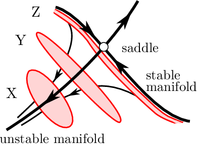
The domain $D$ is very thin, as shown in Fig. 5A. This is related to the $\lambda$-lemma, one of the most important theorems in the theory of dynamical systems [35]. From this theorem, we can say the following:

• •

  A region intersecting the unstable manifold of a saddle equilibrium point moves toward the stable manifold of the saddle when the region is moved by the flow that is backward in time;

• •

  When the region comes close to the stable manifold, the region becomes thin due to the hyperbolic behavior near the saddle.

Figure 9 illustrates how a region X moves and is deformed into thinner regions Y and Z through the backward flow. As shown in Fig. 2B, $D$ is obtained by the intersection of $T(H)$ and the backward orbit whose initial point is in $H$. Therefore, $D$ becomes thin along the center stable manifold, as shown in Figs. 5A and 9.

Since the sequence of the inverse images $S^{-n}(D)\ (n=1,2,\ldots)$ approximates the basin of attraction, it is important to clarify how the geometric structure of the inverse images is constructed, and hence clarify the shape of the basin of attraction.

First, we discuss why $S^{-1}(D)$ is V-shaped in the thin region $D$, as shown in Fig. 6. Since $S^{-1}(D)=U^{-1}(T^{-1}(D))$, we show below how the shape of $T^{-1}(D)$ is deformed by $U^{-1}$.

The inverse image $S^{-2}(D)$ has a slit due to a mechanism similar to the one discussed in the previous section. Since $S^{-2}(D)=U^{-1}(T^{-1}(S^{-1}(D)))$, we consider two steps, $T^{-1}(S^{-1}(D))$ and $U^{-1}(T^{-1}(S^{-1}(D)))$. Here, $T^{-1}(S^{-1}(D))$ is obtained by the backward image of $S^{-1}(D)$, and it is contained in $T^{-1}(D)$, as shown by the blue region in Fig. 14C. This region is moved by $U^{-1}$; it is expanded along the direction of the stable manifold and contracted along the direction of the unstable manifold, as with $T^{-1}(D)$. As a result, $S^{-2}(D)$ becomes V-shaped with a slit, as shown in Fig. 14D. We can also give a similar explanation for the stripe pattern, which is formed by the repeated expansion of nested regions.

In the above discussion, we clarified the mechanism that shapes the basin of attraction. Although the parameter $\gamma$ induces a period-doubling cascade to chaos, the mechanism for constructing the basin of attraction is the same and does not depend on $\gamma$. The domain, the inverse images of the domain, and the basin of attraction have only slight continuous changes, as shown in Fig. 8. Figures 15A and B show the basin of attraction and the chaotic attractor for $\gamma=0.0187$ and $0.01903$, respectively, before the attractor disappears. As $\gamma$ increases, the attractor expands to reach the boundaries of the basin of attraction. When the attractor contacts the boundaries of the basin of attraction (red arrows in Fig. 15B), the attractor breaks down, and the model no longer continues walking. In the theory of dynamical systems, this phenomenon is known as the boundary (attractor) crisis [36].

References

- [1] G. A. Cavagna, F. P. Saibene, and R. Margaria, “External work in walking,” Journal of Applied Physiology, vol. 18, no. 1, pp. 1–9, 1963.
- [2] G. A. Cavagna and R. Margaria, “Mechanics of walking.,” Journal of Applied Physiology, vol. 21, no. 1, pp. 271–278, 1966.
- [3] G. A. Cavagna, N. C. Heglund, and C. R. Taylor, “Mechanical work in terrestrial locomotion: two basic mechanisms for minimizing energy expenditure,” American Journal of Physiology - Regulatory, Integrative and Comparative Physiology, vol. 233, no. 5, pp. R243–R261, 1977.
- [4] N. Ogihara, S. Aoi, Y. Sugimoto, K. Tsuchiya, and M. Nakatsukasa, “Forward dynamic simulation of bipedal walking in the japanese macaque: Investigation of causal relationships among limb kinematics, speed, and energetics of bipedal locomotion in a nonhuman primate,” American Journal of Physical Anthropology, vol. 145, no. 4, pp. 568–580, 2011.
- [5] R. Alexander, “Mechanics of bipedal locomotion,” in Perspectives in Experimental Biology 1 (P. Spencer-Davies, ed.), pp. 493–504, Oxford: Pergamon Press, 1980.
- [6] S. Mochon and T. A. McMahon, “Ballistic walking,” Journal of Biomechanics, vol. 13, no. 1, pp. 49–57, 1980.
- [7] S. Mochon and T. A. McMahon, “Ballistic walking: an improved model,” Mathematical Biosciences, vol. 52, no. 3-4, pp. 241–260, 1980.
- [8] A. D. Kuo, “A simple model of bipedal walking predicts the preferred speed-step length relationship,” ASME Journal of Biomechanical Engineering, vol. 123, no. 3, pp. 264–269, 2001.
- [9] A. D. Kuo, “Energetics of actively powered locomotion using the simplest walking model,” ASME Journal of Biomechanical Engineering, vol. 124, no. 1, pp. 113–120, 2001.
- [10] M. Srinivasan and A. Ruina, “Idealized walking and running gaits minimize work,” Proceedings of the Royal Society of London A: Mathematical, Physical and Engineering Sciences, vol. 463, no. 2086, pp. 2429–2446, 2007.
- [11] J. H. Macdonald, “Lateral excitation of bridges by balancing pedestrians,” Proceedings of the Royal Society of London A: Mathematical, Physical and Engineering Sciences, vol. 465, no. 2104, pp. 1055–1073, 2009.
- [12] S. Fujiki, S. Aoi, T. Funato, N. Tomita, K. Senda, and K. Tsuchiya, “Adaptation mechanism of interlimb coordination in human split-belt treadmill walking through learning of foot contact timing: a robotics study,” Journal of The Royal Society Interface, vol. 12, no. 110, 2015.
- [13] T. McGeer, “Passive dynamic walking,” The International Journal of Robotics Research, vol. 9, no. 2, pp. 62–82, 1990.
- [14] T. McGeer, “Dynamics and control of bipedal locomotion,” Journal of Theoretical Biology, vol. 163, no. 3, pp. 277–314, 1993.
- [15] F. Asano, Z.-W. Luo, and M. Yamakita, “Biped gait generation and control based on a unified property of passive dynamic walking,” IEEE Transactions on Robotics, vol. 21, no. 4, pp. 754–762, 2005.
- [16] S. M. Bruijn, D. J. J. Bregman, O. G. Meijer, P. J. Beek, and J. H. van Dieën, “The validity of stability measures: A modelling approach,” Journal of Biomechanics, vol. 44, no. 13, pp. 2401–2408, 2011.
- [17] T. Chyou, G. F. Liddell, and M. G. Paulin, “An upper-body can improve the stability and efficiency of passive dynamic walking,” Journal of Theoretical Biology, vol. 285, no. 1, pp. 126–135, 2011.
- [18] S. Russell, P. Sheth, and K. P. Granata, “Virtual slope control of a forward dynamic bipedal walker,” ASME Journal of Biomechanical Engineering, vol. 127, no. 1, pp. 114–122, 2005.
- [19] M. J. Coleman and A. Ruina, “An uncontrolled walking toy that cannot stand still,” Physical Review Letters, vol. 80, no. 16, pp. 3658–3661, 1998.
- [20] S. Collins, A. Ruina, R. Tedrake, and M. Wisse, “Efficient bipedal robots based on passive-dynamic walkers,” Science, vol. 307, no. 5712, pp. 1082–1085, 2005.
- [21] S. H. Collins, M. Wisse, and A. Ruina, “A three-dimensional passive-dynamic walking robot with two legs and knees,” The International Journal of Robotics Research, vol. 20, no. 7, pp. 607–615, 2001.
- [22] A. Goswami, B. Thuilot, and B. Espiau, “A study of the passive gait of a compass-like biped robot: Symmetry and chaos,” The International Journal of Robotics Research, vol. 17, no. 12, pp. 1282–1301, 1998.
- [23] T. R. Johnston and M. Hubbard, “Optimization of the visco-elastic parameters describing the heel-region of a prosthesis,” Journal of Theoretical Biology, vol. 311, pp. 1–7, 2012.
- [24] A. D. Kuo, “Stabilization of lateral motion in passive dynamic walking,” The International Journal of Robotics Research, vol. 18, no. 9, pp. 917–930, 1999.
- [25] M. J. Kurz, T. N. Judkins, C. Arellano, and M. Scott-Pandorf, “A passive dynamic walking robot that has a deterministic nonlinear gait,” Journal of Biomechanics, vol. 41, no. 6, pp. 1310–1316, 2008.
- [26] M. Kwan and M. Hubbard, “Optimal foot shape for a passive dynamic biped,” Journal of Theoretical Biology, vol. 248, no. 2, pp. 331–339, 2007.
- [27] P. E. Roos and J. B. Dingwell, “Influence of simulated neuromuscular noise on movement variability and fall risk in a 3D dynamic walking model,” Journal of Biomechanics, vol. 43, no. 15, pp. 2929–2935, 2010.
- [28] J. L.-S. Su and J. B. Dingwell, “Dynamic stability of passive dynamic walking on an irregular surface,” ASME Journal of Biomechanical Engineering, vol. 129, no. 6, pp. 802–810, 2007.
- [29] M. Garcia, A. Chatterjee, A. Ruina, and M. Coleman, “The simplest walking model: Stability, complexity, and scaling,” ASME Journal of Biomechanical Engineering, vol. 120, no. 2, pp. 281–288, 1998.
- [30] A. L. Schwab and M. Wisse, “Basin of attraction of the simplest walking model,” in ASME Design Engineering Technical Conferences, 2001.
- [31] T. de Boer, M. Wisse, and F. C. T. van der Helm, “Virtual slope control of a forward dynamic bipedal walker,” ASME Journal of Biomechanical Engineering, vol. 132, no. 7, p. 071012, 2010.
- [32] H. Gritli, N. Khraief, and S. Belghith, “Period-three route to chaos induced by a cyclic-fold bifurcation in passive dynamic walking of a compass-gait biped robot,” Communications in Nonlinear Science and Numerical Simulation, vol. 17, no. 11, pp. 4356–4372, 2012.
- [33] H. Gritli, S. Belghith, and N. Khraeif, “Intermittency and interior crisis as route to chaos in dynamic walking of two biped robots,” International Journal of Bifurcation and Chaos, vol. 22, no. 03, p. 1250056, 2012.
- [34] Q. Li and X.-S. Yang, “New walking dynamics in the simplest passive bipedal walking model,” Applied Mathematical Modelling, vol. 36, no. 11, pp. 5262–5271, 2012.
- [35] C. Robinson, Dynamical systems: Stability, symbolic dynamics, and chaos. Studies in Advanced Mathematics, Boca Raton, FL: CRC Press, 2008.
- [36] C. Grebogi, E. Ott, and J. A. Yorke, “Crises, sudden changes in chaotic attractors, and transient chaos,” Physica D, vol. 7, no. 1-3, pp. 181–200, 1983.
- [37] Y. Suzuki, T. Nomura, M. Casadio, and P. Morasso, “Intermittent control with ankle, hip, and mixed strategies during quiet standing: A theoretical proposal based on a double inverted pendulum model,” Journal of Theoretical Biology, vol. 310, pp. 55 – 79, 2012.
- [38] Y. Asai, Y. Tasaka, K. Nomura, T. Nomura, M. Casadio, and P. Morasso, “A model of postural control in quiet standing: Robust compensation of delay-induced instability using intermittent activation of feedback control,” PLoS ONE, vol. 4, p. e6169, 07 2009.
- [39] T. Funato, S. Aoi, N. Tomita, and K. Tsuchiya, “Smooth enlargement of human standing sway by instability due to weak reaction floor and noise,” Royal Society Open Science. in press.