Generalization of the Fedorova-Schmidt method for determining particle size distributions
Abstract
One reports the integral transform that determines the particle size distribution of a given sample
from the small-angle scattering intensity under the assumption that the particle correlation
function is a polynomial of degree . The Fedorova-Schmidt solution [J. Appl. Cryst.
11, 405, (1978)] corresponds to the case . The procedure for obtaining a
polynomial approximation to a particle correlation function is discussed and applied
to the cases of polidisperse particles of tetrahedral or octahedral or cubical shape.
Synopsis: It is reported the integral transform that determines the particle size distribution
from the small angle scattering intensity under the assumption that the particle correlation
function is a polynomial.
Keywords: polidisperse samples, size distribution determination, small-angle scattering,
polyhedral particles.
1 Introduction
Colloidal suspensions, demixing alloys, porous glasses, carbons are classical examples of materials that have a particulate structure on a length scale of 1-nm. For these samples scattering data can successfully be used to determine the particle size distribution in the favorable cases where: a) the constituting particles and the surrounding medium are fairly homogeneous on a spatial resolution of 1nm, b) the sample particles have the same geometrical shape and are isotropically distributed, and c) interference effects among different particles are negligible. The application of this procedure to small-angle scattering (SAS) intensities traces back to the contributions of Roess(1946) and Roess & Shull (1947). In particular, Roess & Shull devised an early scheme whereby the particle size distribution could be found by comparing the observed SAS intensity with plots of theoretical intensities numerically evaluated by considering reasonable particle shape and appropriate size-distribution functions. Besides, Roess (1946) also showed that the size distribution can be expressed as an integral transform of the observed intensity in the case of spherical shape. This interesting result was improved and successfully applied by Letcher & Schmidt(1966) to get the particle size distributions of three Ludox samples by the analysis of their small-angle x-ray (SAXS) intensities. Some years later Fedorova & Schmidt (1978) generalized the previous result showing that the size distribution can be expressed as an integral transform of the SAS intensity for all the particle shapes characterized by an isotropic form factor of the following form
| (1) |
where is the scattering vector (
denoting the particle beam wave-length and the
scattering angle),
denotes the maximal chord of the particle, its volume,
and depend on the particle shape and dimensionality,
and is the Bessel function of the 1st kind. The shapes
allowed by this more general formulation include hollow spheres, disks of
negligible thickness and uniform or hollow cylinders of infinite length.
Besides, in all these cases, Fedorova and Schmidt worked out the integral
transform that yields the size distribution from the SAS
intensity collected with the pin hole or the infinite slit geometry.
The main aim of this paper is to get a generalization of this result.
In fact, it will be shown that the size distribution can be written as an
integral transform of the collected intensity in all the cases where the particle
correlation function is an degree polynomial continuous,
together with its first derivatives, throughout .
Consider a particle of maximal chord . The correlation function (CF)
of this particle identically vanishes once exceeds . Hence, the
above assumption of continuity is equivalent to state that the CF and its
first derivatives vanish at .
The plan of the paper is as follows. For completeness, section 2 reports
the expression of the correlation function (CF) in terms of the so-called stick
probability functions (Debye et al. 1957; Goodisman & Brumberger, 1971) while
§ 3 expresses the observed scattering intensity in terms of the particle CF, the
particle size distribution and a further contribution related to the overlapping of
different particles. The Fourier transform of this contribution, on the average,
negatively contributes to the observed scattering intensity and vanishes in the infinite dilution limit. Hence, as firstly pointed out by Guinier and Fournet (1955), the
relation exploited by polidisperse analysis is physically consistent only for
highly diluted samples. Sections 4 and section 5 respectively report the
generalization of the Fedorova-Schmidt result in direct and in reciprocal space.
Section 6 first discusses how to construct a polynomial approximation of a particle CF, and then, in §6.1, 6.2.1 and 6.2.2, analyzes the cases of the sphere, the cube/octahedron and the
tetrahedron.
The final conclusions are reported in § 7.
2 Stick probability functions and correlation function
The scattering intensity is the square modulus of the Fourier transform (FT) of , the scattering density of the sample. In the SAS domain, is fairly approximated by a two value function that can therefore be written as
| (2) |
where () denotes the scattering density of phase 1 (2) and defines the full geometry of phase 1 since it is equal to 1 or 0 depending on whether the tip of falls inside or outside phase 1. (The definition of is quite similar.) The spatial region occupied by the th phase will be denoted as and its volume by . The volume of the sample is and the ratio is the volume fraction of the th phase. According to Debye et al.(1957) the stick probability function relevant to the th and th phase is defined as
| (3) |
Here is a unit vector that spans all possible directions. Function is the angular average of the volume fraction of the overlapping region between phases and , once the latter has been translated by . It also represents the probability that a stick of length , after having been randomly tossed a very large number of times, falls with one end inside phase and the other end within phase . The s have the following properties [ Goodisman & Brumberger (1971), Ciccariello et al.(1981), Ciccariello (1984)]
| (4) |
| (5) |
| (6) |
| (7) |
Here the prime denotes the derivative, the area of the interphase surface,
the length of the th edge present on the interface, the associated dihedral angle. Further, in (7), and respectively denote the mean and the Gaussian curvature of the interface at the point and a further contribution that is only present when the interphase surface presents edges meeting at some vertices. We defer to Kirste and Porod (1962) for the derivation of
the integral contribution and to Ciccariello & Sobry (1995) for the explicit expression
of .
For a statistically isotropic sample one finds that [Debye et al.(1957), Goodisman &
Brumberger (1971), Ciccariello et al.(1981)] the scattering intensity is
| (8) |
with
| (9) |
where is the mean square scattering density fluctuation, i.e.
| (10) |
with . Function is commonly referred to as the correlation function of the sample. By equation. (4b) it takes the form
| (11) |
more useful in our later analysis. From (5) and (11) immediately follows that
| (12) |
Similarly, the expressions of and are also
known by Equation.s (6) and (7).
Multiplying by , integrating over all the positive s and
using Equation. (8) and (12a), one finds the so-called Porod invariant relation
| (13) |
3 The scattering intensity in the polidisperse approximation
Consider now the case of a particulate sample where the particles have the same shape and different sizes. The distribution of the particles in the space is assumed to be statistically isotropic. The phase formed by the particles will be named phase 1. Hence becomes equal to
| (14) |
where the sum runs over all the particles, labelled by index and denotes now the characteristic function of the th particle. The substitution of (14) into the definition [see equation (3)] yields
| (15) |
with
| (16) |
| (17) |
and denoting the volume of the th particle.
The sum on the right hand side (rhs) of (15) and function respectively are the intraparticle and the interparticle contributions to . The last contribution is poorly known. One knows that it and its first derivative vanish as (because the overlapping between two different particles is possible only if is greater than the lowest of the particle maximal chord values) and that it approaches as becomes very large (because the probability that the stick of length has
its ends within phase 1 is equal to ).
We elaborate now the intraparticle contribution. To this aim
one observes that function
is independent on the actual position and orientation of the particle and only
depends on the shape (fixed by assumption) and the size of the particle. It is the (isotropic) correlation function of the th particle. It is equal to zero as exceeds , the largest chord of the particle, and is equal to one at . Comparing with , it results that .
Then, denoting by the CF of the unit particle, namely the particle having its largest chord equal to the unit length, one has
| (18) |
The volume of the th particle is and the first sum on the rhs of (15) becomes
| (19) |
where the sum runs now over the particles’ different sizes labelled by . Moreover, we have denoted by the number of particles with the th size, and by the total number of the particles present in the sample. As becomes infinitely large, becomes equal to , the particle number mean density of the sample and, what is more important, since runs over a very large number, can be approximated by the infinitesimal quantity where represents the probability density of finding a particle of size within the interval ]. Then, the first sum on the rhs of (15) converts into an integral, i.e.
| (20) |
From equations (11)) and (15) one finds that the sample CF is the sum of two terms
| (21) |
with
| (22) |
and
| (23) |
The CF’s definition requires that . Setting into (22) and observing that the particle mean volume is given by
| (24) |
so that , one finds that
| (25) |
Since , one also finds that
| (26) |
From (25) and (26) one concludes that neither nor are CFs and that the only shares this property because . By Fourier transforming relation (21), multiplied by , and putting
| (27) |
one finds that the scattering intensity, given by (8), separates into two contributions, i.e.
| (28) |
with
| (29) |
and
| (30) |
and respectively represent the intraparticle and the interparticle contribution to the scattering intensity. It is noted that Guinier & Fournet (1955) first discussed the importance of the contribution , which was mainly analyzed in the molecular approximation. Apply now the basic relation
| (31) |
to and . One respectively finds
| (32) | |||
and
| (33) | |||
The negativeness of implies that is negative in some -ranges so that is not a scattering intensity but only a FT. Owing to the fact that also tends to zero as , it follows that decreases faster than as . One concludes that the asymptotic behaviour of is equal to that of . The last one immediately follows from (29) and from the fact that , where denotes the surface area of the unit particle. One finds that Porod’s law (Porod, 1951) takes the form
| (34) |
with
| (35) |
denoting the particle mean surface area, and .
Moreover, the only sum of (32) and (33) yields the correct Porod invariant [i.e. (13)].
The polidisperse approximation consists in setting and
neglecting (Guinier & Fournet, 1955; Feigin & Svergun, ; Gille, 2013). The approximation is certainly correct at large s for the behaviour of .
The last contribution is only appreciable at small s where the approximation consequently fails unless the sample is very dilute, because
vanishes as 11
1
A heuristic way for overcoming the high dilution assumption consists in assuming that has a known parameterized form, for instance , which vanishes together
with its derivative as and tends to as . Then is obtained by (23), by (30) and is
known (in terms of and by the relation . Finally the four
relations (13), (32), (33) and (34) in principle determine, , , and . . Only in this case
fairly fulfills the Porod invariant relation because the rhs of (32) closely approaches .
Finally, it is observed that the knowledge of
, and only determines since one has .
From the last equality one obtains that which tests the accuracy of .
4 Generalization of the Fedorova-Schmidt method
Hereafter it will be assumed that the approximation holds true and the problem of obtaining an integral transform that directly determines from the scattering intensity will now be tackled. In principle, if is known throughout the full -range, function , defined as
| (36) |
also is fully known. On the other hand, by equation (29) one finds that
| (37) |
Combining (36) and (37) and putting, for notational simplicity,
| (38) |
one gets the integral equation
| (39) |
which, once solved, determines , and hence via (38), in terms of , and hence of via (36). Using the property that identically vanishes if , equation (39) converts into
| (40) |
Our task now is that of showing that the (integral) transform that expresses in terms and can be explicitly written down if one assumes that:
- •
i) is an th degree polynomial, i.e.
(41) with and ,
- •
ii) and its first derivatives (with ) vanish at , i.e. after putting
(42) one assumes that
(43) - •
iii) exponentially decreases as and, as , it goes to zero sufficiently fast for the later considered integrals to exist.
Owing to assumption ii), from (40) follows that
| (44) |
For the th derivative one can no longer use (43) and one finds that
| (45) |
Up to the th order, the successive derivatives have a similar structure. The th derivative however will involve no integral contribution because the integrand vanishes owing to assumption i). In this way one finds that must obey the following linear inhomogeneous differential equation
| (46) |
If the sum on the left hand side reduces to a single term so that is simply determined by
| (47) |
If , Equation. (46) is a genuine differential equation of
order yielding as one of its solutions.
To get one must first determine
the general integral of the associated homogeneous differential equation
| (48) |
then find a particular integral of (46) and, finally, impose the appropriate
boundary conditions.
Looking for a solution of (48) of the form one finds
| (49) | |||
Using the descending Pochhammer symbol , defined as if and if , equality (49) becomes
| (50) |
It is a polynomial equation of degree in unknown . For simplicity one assumes that the roots are distinct. (The case where some roots coincide will be discussed later.) The general integral of Equation. (48) is
| (51) |
where are arbitrary constants.
A particular integral of the non-homogeneous differential equation
(46) is easily obtained by the Cauchy method [see
§39 of Goursat (1959)]. It reads
| (52) |
where is an arbitrarily chosen value and functions are the solutions of the following system of linear equations
| (53) | |||||
that reduces to if . The s solutions of this system are
| (54) |
and function reads
| (55) |
where it has been put
| (56) |
and if .
The proof that function , defined by Equation. (52), is a solution of differential equation (46) and that (55) is a solution of (53) is reported in appendix A.
The general integral of Equation. (46) is and the sought
for particle probability density has the form
Condition iii) is fulfilled if one chooses and In this way the sought for integral transform that allows one to obtain the particle size probability density from is fully determined and reads
| (57) |
Finally, the case of degenerate roots can rigorously be dealt with by the procedure described in §3.3 and 3.4 of Bender & Orszag (1978). In practice one can also proceeds, more simply, as follows. Let be a group of coinciding roots. One removes the degeneracy by the substitutions with and equal to a very small number and then apply the described procedure for determining . By continuity the resulting error will be small with because all the above reported expressions continuously depend on the s. Hereafter one will confine himself to the non degenerate case.
5 The resolvent kernel in reciprocal space
The integral transform that determines by the observed scattering intensity is immediately obtained by taking the derivative of the rhs of (36) and substituting the result into (57). The result is
| (58) |
where denotes the derivative operator with respect to .
This result generalizes the Fedorova Schmidt formula because it applies to any CF that
has a polynomial form as it happens in the case of spheres. It is noted that the
reconstruction of from the observed intensity, under the assumption of a
polynomial CF, holds also true in the case of the slit collimation thanks to
Guinier’s integral transform (Guinier, 1946) that converts , the intensity collected with the slit geometry, into the pin-hole .
Our task now is that of rewriting (58) in a more compact form that is more convenient for numerical evaluation. To this aim one formally exchanges the integration order in (58) and, after putting
| (59) |
one gets
| (60) |
It is noted that definition (59) does not always lead to an existing because, according to Riemann’s theorem (Bender & Orszag, 1978), the integral exists only if , a condition that is not a priori ensured. However each integral contributing to equation (57) exists owing to assumption iii). Consequently the convergence difficulty of (59) is related to the fact that the integration order cannot be exchanged for the s such that . Hence one must handle the case differently from that where . This will be respectively done in the following two subsections.
5.1 The case
Assume, for simplicity, that all the s are greater than . In this case the order of integration is not important and the corresponding s do exist. These can be expressed in terms of some known transcendental functions proceeding as follows. Perform the integration variable change in (59) and momentarily omit index for notational simplicity. One gets
| (61) |
Putting , using the identity [Luke, § 2.9, (1969)]
| (62) |
and denoting the derivation operator with respect to by , the previous integral becomes
Recalling the definition of , the generalized Fresnel sine integral (equation (6.5.8) of Abramowitz & Stegun, 1970), one finds that
| (63) |
which can also be expressed in terms of the hypergeometric function (Luke, 1969) as
| (64) |
Combining equations (60), (61), (62) and (63) one finds
| (65) |
with
| (66) |
For later convenience it is also mentioned that the leading asymptotic expansion of at large s is
| (67) | |||||
5.2 The case
One assumes that all the s are smaller than . In this case, as it was already said, the convergence at of each integral present in (57) is ensured by the sufficiently fast decrease of . Hence, one writes
| (68) |
with
| (69) |
Owing to condition iii), the limit of as cannot be divergent. Then, from equation (57), it follows that whatever . Expressing in terms of its FT and omitting index for simplicity, one finds
The order of integration can now be exchanged. Using again identity (62) the last integral becomes
| (70) |
A further change of the integration variable converts the above -integral into
| (71) |
This integral also can be expressed in terms of an hypergeometric function, since
| (72) | |||||
i.e. the opposite of the hypergeometric contribution present in the rhs of (64). It follows that, at large
, the leading asymptotic term of is the opposite of that of
[see (67)] plus .
Combining equations (68)-(72) and substituting the result in (58) one finds that
| (73) |
with
| (74) |
5.3 The general case of some s smaller and the others greater than
The expression of the integral transform that determines the particle size distribution from the scattering intensity, whatever the values, immediately follows from (66) and (74). It is
| (75) |
with
| (76) |
where the ′ and the ′′ respectively denote that the corresponding sums are restricted to
s greater and smaller than , and .
Owing to assumption iii) the behaviour of the general resolvent kernel
is such as to ensure the convergence of (75)
even though the property does not apply to each term of the sums. Further,
the convergence is rather weak as it will appear clear from the discussions reported in the following section.
6 Polynomial approximation of the CF
At this point one wonders: besides the spherical shape, do exist other particle shapes that have a polynomial CF? As yet the answer is unknown. But this does not imply that one cannot use the above finding to approximate the CF of particles with a given shape by a polynomial. To construct such approximations one first recalls that , the CF of a unit particle with a given shape, obeys some general constraints. The simplest of these are:
- •
a) ,
- •
b) with ( will be hereafter referred to as specific surface),
- •
c) ,
- •
d) ,
- •
e) 4,
- •
f) 4 where denotes the Guinier gyration radius of the particle,
- •
g) where is the particle angularity defined by equation (6) (Porod, 1967; Méring and Tchoubar, 1968; Ciccariello et al.; 1981), and
- •
h) where , defined by equation (7), is the particle curvosity (Kirste & Porod. 1962; Ciccariello & Sobry, 1995).
Besides the listed constraints one might consider other ones. For instance, if the particle shape is such that one does not have a parallelism condition between finite area subsets of the particle surface at a relative distance equal to the particle maximal chord, one also has . Similarly, e) and f) are particular cases of the general relation
| (77) | |||||
that connects the th moment of the particle CF to the higher order gyration radii
of the particle (see Appendix B for the proof of (77) and for the explanation of
the symbols there involved).
According to Shannon’s theorem the information content
of any SAS intensity is not particularly rich so that a ten of parameters only can be determined
(Moore, 1980; and Taupin & Luzzati, 1982). Thus, in performing a polidisperse
analysis of the SAS intensity of a given sample, it appears sensible to approximate
the particle CF by a polynomial that fulfills some of the above constraints.
In this paper the simplest cases of the third [] and fourth [] degree polynomial approximations will be considered. In particular, it will be required that the polynomial
approximation obeys a), b), c) and d) that explicitly accounts for the support
properties of the CF, the normalization at and a single geometrical feature of the
particle, namely its specific surface . For the 3rd degree case one finds that
| (78) |
The associated angularity, curvosity, volume and Guinier gyration radius respectively are
| (79) | |||||
From (78) follows that the coefficients, defined by (42), are
| (80) |
One clearly has , , and the solution of polynomial equation (50) is
| (81) |
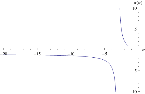
Figure 1 plots vs. . It is recalled that must be such that because, at fixed volume, the sphere is the geometric solid
that has the smallest surface. Thus, varies between and
and the variation is very sharp around .
In the following subsections we shall analyze the case of the
sphere, that of the cube and the octahedron, that of the tetrahedron and, finally, that of the
4th degree approximation.
6.1 The sphere case
This case, already fully exploited, is mainly reported in order to make fully evident that equations (75) and (76) coincide with those of Fedorova and Schmidt. As it was just said the specific surface of the sphere is . The substitution of this value in (78) reproduces the exact CF of the unit sphere, i.e.
| (82) |
This nice property implies that the constraints relevant to the angularity, the curvosity and all the Guinier higher order gyration radii [see (79)]
are exactly obeyed.
As already anticipated it is now shown that integral transform (57) coincides with
Fedorova and Schmidt’s one in the case of spherical particles. From Eqs. (80)
and (81) it follows that and . Hence Equation. (57) reads
| (83) |
Integrating twice by parts, one obtains
| (84) |
that coincides with the result of Letcher and Schmidt (1966) and Fedorova
& Schmidt (1978).
It is instructive to check equations (57) and (58)
choosing as size probability density the Poisson one, namely
| (85) |
with and . In the sphere case, the explicit evaluation of (37) yields
| (86) |
Substituting this expression in the rhs of (84) one straightforwardly
verifies that the result coincides with .
The check of (58) is more interesting. Since , the size distribution
is determined by (65) and (66). The resolvent kernel , now
denoted as , is
| (87) |
with
| (88) |
and (65) becomes
| (89) |
Function is such that the integral can be set equal to zero as because at large it behaves as that, it being wildly oscillating if , averages to zero. Hence, equation (89) can be written in the well known form
| (90) |
which converges faster than (89) at . Its correctness can explicitly be checked in the case of a (4,1) Poisson distributed spherical particles. The explicit form of is obtained by (29) and reads
| (91) |
From this expression one finds that . Substituting these expressions in the rhs of (90) and evaluating the integral one correctly finds function . It is stressed that (90) numerically is much more convenient than (58) to get from the observed scattering intensity. [A more convenient form has been recently discussed by Botet & Cabane (2012).] Finally, figure 2 shows the size distribution obtained by the numerical evaluation of (90) using as the values resulting from the numerical integration of (29) in the sphere case (with ).

6.2 The 3rd degree polynomial approximation of the cube’s, octahedron’s and tetrahedron’s CFs
Ciccariello and Sobry (1995) showed that the CF of any polyhedral particle is a 3rd degree
polynomial in the innermost -range. This condition clearly is obeyed by the known
CFs of the regular tetrahedron, octahedron (Ciccariello, 2014) and cube (Goodisman, 1980). In these cases the innermost -range is larger than half the total -range where the CFs differ from zero. For this reason it is tempting to approximate the known CFs by a 3rd degree polynomial, vanishing together with its first derivative at the outermost value and subsequently perform a polidisperse analysis along the lines expounded in §6.1.
The results of this approximation will now be illustrated.
One knows that the specific surface values of the unit cube, the unit octahedron and the unit tetrahedron are respectively equal to
| (92) |
The 3rd degree polynomial approximations of the three CF immediately result from
the substitution of the above values into (78).
Since the values of the cube and the octahedron coincide the resulting 3rd degree approximation of the cube CF is equal to that of the octahedron.


Figure 3 plots the exact CFs and their 3rd degree approximations as well as the FTs
of the exact and the polynomial approximated CFs. In direct space the agreement
is relatively good for the tetrahedron, reasonable for the cube and not bad for the
octahedron since small discrepancies are only present in the outermost /range.
These discrepancies are responsible for those observed at small ’s in reciprocal
space. They can be reduced requiring that the polynomial
approximations also obey
constraint e) because the fulfillment of this constraint implies that the
FTs of the exact and the polynomial approximated CFs coincide at .
To do that one must consider a 4th degree polynomial approximation, a case
discussed in §6.3.
We shall go on with the discussion of the 3rd degree
polynomial approximation in the cases of the (4,1) Poisson distributions of cubes, octahedra
or tetrahedra. in order to make clear all the point of the analysis.
By Equation. (78) one finds that function , defined by Equation. (40), becomes
| (93) | |||||
Its 3D FT, multiplied by , yields the polidisperse scattering intensity, i.e.
| (94) | |||||
Substituting in the above two relations the values reported in Equation.(92) one obtains the CFs as well as the scattering intensities relevant to the three collections of Poisson polidisperse tetrahedrons, octahedrons and cubes. The corresponding exact values are obtained, using the exact particle CFs, by a numerical evaluation of integrals (40) and (29), which can more conveniently be evaluated by
| (95) |
with
| (96) | |||


The results are shown in Figure. 4. The left panel shows the ’s and the right
one the intensities and their Porod plots. For the intensities, the quality of the agreement is similar to that shown in Fig. 3. However, the Porod plots show that the intensity discrepancies observed near the origin are washed out by the factor . Some discrepancies are still observed around in the only cubic and octahedral cases, while the agreement is quite satisfactory in the tetrahedron case.
6.2.1 Determination of the size distribution from the scattering intensity in the cube/octahedron case
The root of the resolvent equation relevant to the 3rd degree polynomial approximation of a particle CF is given by equation (81). Since the specific surfaces of the unit octahedron and the unit cube coincide it follows that is the same in the two case. It will be denoted by . Recalling that is equal to [see (92)], one finds
| (97) |
The resolvent kernel (66) takes now the form , with
| (98) | |||||
and . Also in this case one finds that in the sense reported just below (89), so that (65) can be written as
| (99) |
that is more convenient for numerical computation because the integrand behaves
as at large s.
The result (99) has been analytically checked substituting, in its rhs, with
given by expression (94) and setting . The result is the outset Poisson (4,1) size
distribution.
6.2.2 Determination of the size distribution from the scattering intensity in the tetrahedron case
The specific surface of the tetrahedron is given by (92c). Then the root of the resolvent equation associated to the polidisperse polynomial approximation of tetrahedrons is given by (81) and reads
| (100) |
It is smaller than one and therefore one must apply the results of §5.2. The resolvent kernel, defined by (74), is with
| (101) | |||||
also is such that in the weak sense. One concludes that the particle size distribution in the tetrahedron polynomial approximation is given by
| (102) |
The analytic check of this relation is fully satisfactory as for the case of equation (99) .

As in the case of Fig. 2, equations (99) and (102) have also been numerically checked as follows. First one evaluates the scattering intensity,
given by equation (94), for the octahedron/cube and the tetrahedron cases
on a grid of 1000 points uniformly covering the interval . Then one evaluates
integrals (98) and (101) using an -grid of 40 values uniformly
distributed over the interval [0, 20]. The resolvent kernels (including the sphere case) are plotted in figure 5 and the resulting size distributions are shown in Fig. 2. The agreement
is quite satisfactory since the discrepancies observed at small s are related to
the truncation. For a general discussion of this point see Pedersen (1994).

The s have also been reconstructed, along the lines just reported, using as scattering intensities those obtained by the exact particle CFs, i.e. using equations (95) and (96). The results are shown in figure 6, where the blue full circles, the magenta full squares and the golden full diamonds respectively refer to the polidisperse octahedra, cubes and tetrahedra. The figure represents a first test on the reliability of approximating an exact CF by a polynomial one to perform a polidisperse analysis. It shows that the resulting is reliable if the particle exact scattering intensity is reasonably approximated by the polynomial polidisperse one. It is noted that the agreement must be observed in the Porod plot of the intensities because the inversion formulae involve quantity in their integrands. This appears to be the case of tetrahedral particles, while the 3rd degree polynomial approximation is not equally satisfactory in the case of cubes and octahedra. In fact, one sees that the resulting s are satisfactory in the only outer -range. In the small/medium -range they are not satisfactory because the polynomial polidisperse intensities do not accurately approximate the polidisperse exact ones in the region (see figure 5B).
6.3 The 4th degree polynomial approximation
For greater completeness we shall now briefly report the reasults that are obtained in the cases of (4.1) Poisson distributions of tetrahedrons, octahedrons or cubes when the relevant CFs are approximated by a 4rh degree polynomial . On requires that obeys constraints a), b), c), d) and e). Then one finds that
| (103) |
where and respectively denote the volume and the specific surface of the considered unit polyhedron. The substitution of the and relevant to the unit regular tetrahedron, octahedron and cube yields the 4th degree polynomial approximations of the respective CFs. The left panel of Figure 7 compares the exact CFs to their 4th degree approximations, while the right panel shows the exact and the approximated form factors of the three particle shapes. It is evident that the agreement is far better than in Fig. 3.


The functions , relevant to the (4,1) Poisson polidisperse collections of tetrahedrons, octahedrons and cubes, can algebraically be evaluated by (40), (38) and (103). They can also be Fourier transformed in a closed algebraic form. The results are shown in Figure 8. The comparison with the results reported in Fig. 4 shows that the 4th degree approximation is more accurate than the 3rd degree one even though some discrepancies still survive in the range for the octahedron and cube cases.


We proceed now to apply the generalized Fedorova-Schmidt method. One has and so that . The resolvent equation (50) is a 2nd degree one that can immediately be written down because the coefficients , and are obtained from (103) according to definition (42). The roots are
| (104) | |||
| (105) |
with
| (106) |
Using the and values of the considered three solids one finds
| (107) |
| (108) |
For the three cases, the resolvent kernels are immediately obtained from (76) recalling that . They have the general form and is a function such that its integral over the range becomes weakly equal to zero as . Then the integral transforms that determine the size distributions from the observed intensities have the form of equations (90), (76), (102). Figure 9 shows the results in the cases where the scattering intensities are equal to the FTs of equation (40) with equal to , and and . The agreement is as satisfactory as in the case of the 3rd degree approximation (see figure 2).

Figure 10 shows the resulting size distributions in the cases where the scattering intensities are the FTs of (40) with equal to the exact CFs of the considered three platonic solids. These intensities are the observable ones. Thus Figure 10 shows the accuracy that can be achieved by the 4th degree approximation of the CFs. The comparison of Fig. 10 with Fig. 6 shows the greater accuracy of the 4th degree approximation. The surviving discrepancies are not large enough to make meaningless the application of the generalized Fedorova-Schmidt method to dilute polidisperse real samples of particles with the above considered polyhedral shapes.

7 Conclusions
The main results of this paper are: a) a reformulation of polidisperse analysis based
on the stick probability functions. This presentation should have made more clear the
fact that if the system is not very dilute, the polidisperse analysis is applied to
an intensity that, on the average, is somewhat smaller than the exact ;
b) the derivation of the integral transform that determines the particle size distribution
from the scattering intensity under the assumption that the particles have a polynomial
CFs; c) the procedure for determining an th degree polynomial approximation to
a given CF and finally d) the application of this procedure to (4,1) Poisson distributions
of cubes, octahedrons and tetrahedrons using the lowest significant polynomial
approximations, i.e. the 3rd and the 4th degree ones. For the polynomial approximation
to yield accurate results it is required that be fairly close to ,
where denotes the polidisperse intensity evaluated with the particle’s exact
form factor and the FT of the considered polidisperse polynomial approximation.
Overall the reported results indicate that polidisperse analyses of real scattering data
might be satisfactorily carried through with non spherical particles treated in the
appropriate polynomial approximation.
Appendix A Derivation of equation (52)
It is now proved that function , defined by Equation. (52), is a solution of
differential equation (46).
To this aim it is first observed that equation (46) can be written as
| (109) | |||||
where functions result from the explicit evaluation of the
derivatives present in (46) and, after regrouping the terms, multiplying the
results by . Functions and
also are the general integral and a particular
solution of the homogenous differential equation associated to (109) because
this differs from (48) by a factor.
The first derivative of is easily obtained from Equation. (52) and reads
| (110) | |||||
where the prime denotes the derivative with respect to . Using the first of Equation.s (53) one gets
| (111) |
In a similar way, for , one finds that
| (112) |
The th derivative is
| (113) | |||||
Thus one finds that
| (114) | |||
The expression within the square brackets is equal to zero because is a solution of the homogeneous differential equation. In this way one finds that
| (115) |
and the proof that is a particular integral of Equation. (A.1) is achieved.
It is now proved that (55) are the solution of Equation.s (53).
To this aim one puts for and one writes
as . Equation.s (53)
become
| (116) | |||||
The matrix associated to this system of linear equations is
that, using the expressions, becomes
| (117) |
The determinant of the matrix, formed by the first columns of (117), is the determinant of the coefficients. It is simply evaluated observing that if one multiplies the terms of the th row by for , the th column terms have as common factor. After extracting these factors, determinant reduces to to the Vendermonde determinant
whose value is
| (118) |
To get the expression of coefficient one must evaluate the determinant of the matrix obtained omitting the th column in equation (117) and multiply the result by . The value of determinant is evaluated by the same procedure expounded above. Its value is
| (119) |
where the primes on the sum and product symbols denote that the sum and the product indices cannot be equal to . Dividing this result by and simplifying one gets
| (120) |
that is Equation.(54).
Appendix B Derivation of equation. (77)
First of all the definition of the symbols present in Equation. () are as follows. The prime on the sum denotes that index ranges over the even numbers and that obey the constraint ;
| (121) |
where is the characteristic function of the particle that has its gravity center set at the origin of the Cartesian frame and its maximal chord equal to one and,finally,
| (122) |
The th moment of , using the CF definition, can be written as
| (123) | |||||
One has
| (124) |
with the further constraint , and (123) becomes
| (125) |
where it has been put
| (126) |
and the convention of summing over repeated indices has been adopted. Quantity is a fully symmetric tensor of rank that must behave as a scalar quantity. Hence it has the form
| (127) |
where the expressions must be determined and is a fully symmetric tensor resulting from the sum of terms having the form where is the Kronecker symbol and is a permutation of such that , , …, and . Clearly the existence of requires that be even. If one saturates two indices of , from definition (126) one gets
| (128) |
and by (127) that
| (129) |
Quantity can be explicitly related to . In fact from the definition follows
| (130) |
where symbol means that index is not present. Saturating with in (130), one obtains that
| (131) |
By iteration of this relation one gets
and, since , one finds that
| (132) |
| (133) |
with
| (134) |
To fully simplify the rhs of (125) one must saturate with itself. By relation (133), this amounts to evaluate . This quantity by (130) becomes equal to (it is recalled that )
| (135) |
The second term is equal to , while the third term can be written as
Collecting the above results one finds that
Iterating one gets
| (136) |
Finally, one finds that
| (137) |
Recalling definitions (121) and (122) the proof of (77) is completed.
The relation can easily be checked in the case of a spherical unit particle
since by direct evaluation one finds, from Equation. (82), that
| (138) |
and from (121) that
| (139) |
References
-
Abramowitz, M. & Stegun, I.A. (1970). Handbook of Mathematical Functions, New York: Dover.
-
Bender, C.M. & Orszag, S. A. (1978). Advanced Mathematical Methods for Scientists and Engineers. New York: McGraw-Hill, §3.3 and 3.4.
-
Botet, R. & Cabane, B. (2012). J. Appl. Cryst. 45, 406-416.
-
Ciccariello, S. (1984). J. Appl. Phys. 56, 162-67.
-
Ciccariello, S. (2014). J. Appl. Cryst. 47, in the press; arXiv: 1407.2788v1.
-
Ciccariello, S. & Sobry, R. (1995). Acta Cryst. A 51, 60-69.
-
Ciccariello, S., Cocco, G., Benedetti, A. & Enzo, S. (19881). Phys. Rev. B23, 6474-6485.
-
Debye, P., Anderson, H.R. & Brumberger, H. (1957). J. Appl. Phys. 20, 679-683.
-
Fedorova, I.S. & Schmidt, P.W. (1978). J. Appl. Cryst. 11, 405-11.
-
Feigin, L.A. & Svergun, D.I. (1987). Structure Analysis by Small-Angle X-Ray and Neutron Scattering, (Plenum Press, New York).
-
Gille, W. (2013). Particle and Particle Systems characterization , (CRC Press, London)
-
Goodisman, J. (1980). J. Appl. Cryst. 13, 132-34.
-
Goodisman, J. & Brumberger, H. (1971). J. Appl. Cryst. 4, 347-351.
-
Goursat, E. (1959). Differential Equations. New York: Dover, § 38 and 39.
-
Guinier, A. (1946). Compt. Rend. 223, 161-162.
-
Guinier, A. & Fournet, G. (1955). Small-Angle Scattering of X-rays. New York: John Wiley.
-
Kirste, R. & Porod, G. (1962). Kolloid Z. 184, 1-6.
-
Letcher, J.H. & Schmidt, P.W. (1966). J. Appl. Phys. 37, 649-655.
-
Luke, Y.L. (1969). The Special Functions and Their Approximations, Vol. I, Academic Press:New York.
-
Méring, J. & Tchoubar, D. (1968). J. Appl. Cryst. 1, 153-65.
-
Moore, P.B. (1980). J. Appl. Cryst. 13, 168-175.
-
Pedersen, J.S. (1994). J. Appl. Cryst. 27, 595-608.
-
Porod, G. (1951). Kolloid Z. 124, 83-114.
-
Porod, G. (1967). Small-Angle X-Ray Scattering. Proceedings of the Syracuse Conference, edited by H. Brumberger, 1-8, Gordon & Breach:New York.
-
Roess, L.C. (1946). J. Chem. Phys. 14, 695-697.
-
Roess, L.C. & Shull, C.G. (1947). J. Appl. Phys. 18, 308-313.
-
Taupin, D. & Luzzatti, V. (1982). J. Appl. Cryst. 15, 289-300.