跳到论文正文
W Papers独立论文阅读器 arXiv:1407.5572 论文正文 计算阅读时间 · 0%
引用这篇论文根据当前论文元数据生成,正式投稿前建议核对。


License: arXiv.org perpetual non-exclusive license
arXiv:1407.5572v2 [cs.IT] 20 Aug 2015

Secrecy Capacity Region of Some
Classes of Wiretap Broadcast ChannelsThanks: The material in this paper was submitted in part to the IEEE Information Theory Workshop, Tasmania, Australia, 2-5 November 2014 and the 49th Annual Allerton Conference on Communications, Control, and Computing 2014. This work was accomplished when Meryem Benammar was with the Dept. of Telecommunications at CentraleSupelec.Thanks: Meryem Benammar is with the Mathematical and Algorithmic Sciences Lab, France Research Center, Huawei Technologies Co., Ltd (e-mail: meryem.benammar@huawei.com). Thanks: Pablo Piantanida is with the Laboratoire des Signaux et Systèmes (L2S UMR 8506) at CentraleSupelec-CNRS-Université Paris-Sud, France (e-mail: pablo.piantanida@centralesupelec.fr).Thanks: Copyright (c) 2014 IEEE. Personal use of this material is permitted. However, permission to use this material for any other purposes must be obtained from the IEEE by sending a request to pubs-permissions@ieee.org.

Meryem Benammar and Pablo Piantanida Affiliation:
Abstract

This work investigates the secrecy capacity of the Wiretap Broadcast Channel (WBC) with an external eavesdropper where a source wishes to communicate two private messages over a Broadcast Channel (BC) while keeping them secret from the eavesdropper. We derive a non-trivial outer bound on the secrecy capacity region of this channel which, in absence of security constraints, reduces to the best known outer bound to the capacity of the standard BC. An inner bound is also derived which follows the behavior of both the best known inner bound for the BC and the Wiretap Channel. These bounds are shown to be tight for the deterministic BC with a general eavesdropper, the semi-deterministic BC with a more-noisy eavesdropper and the Wiretap BC where users exhibit a less-noisiness order between them. Finally, by rewriting our outer bound to encompass the characteristics of parallel channels, we also derive the secrecy capacity region of the product of two inversely less-noisy BCs with a more-noisy eavesdropper. We illustrate our results by studying the impact of security constraints on the capacity of the WBC with binary erasure (BEC) and binary symmetric (BSC) components.

I Introduction

Information theoretic secrecy was first introduced by Shannon in his seminal work [1]. He investigates a communication system between a source, a legitimate receiver and an eavesdropper where the source and the legitimate receiver share a secret key. It is shown that, to achieve perfect secrecy, one has to let the key rate be at least as large as the message rate. This result motivated the work [2] by Wyner who introduced the notion of Wiretap Channel. In such a setting, a source wishes to transmit a message to a legitimate receiver in the presence of an eavesdropper but without resorting to a shared key. Besides communicating reliably to the legitimate receiver at a maximum rate, the source has to maximize the equivocation at the eavesdropper so that it cannot recover the message sent over the channel. In the case of perfect secrecy, the conditional probability of the message given the eavesdropper’s observation has to be approximately uniform over the set of messages, i.e., there is no leakage of information to the eavesdropper. The surprising result of Wyner’s work [2] is that the use of a secret key is no longer required to guarantee a positive equivocation rate or even perfect secrecy. Csiszár & Körner’s [3] generalized this result –first derived with the assumption of a degraded eavesdropper– to the general BC and where the source must also transmit a common message to both users. As a matter of fact, an analysis of the corresponding rate region regarding the necessity of two auxiliary random variables, namely, rate splitting and channel prefixing, was carried out by Ozel & Ulukus in [4]. It was shown that under specific channel ordering the rate region requires only one or even none of these variables.

Several multi-terminal Wiretap networks were studied, e.g., the MAC Wiretap Channel has been investigated by Liang & Poor in [5] while physical layer security in broadcast networks was studied by Liang et al. in [6] though, the capacity region is yet to be fully characterized.

Related works

The Wiretap Broadcast Channel (WBC) was first studied under two types of secrecy constraints. The Broadcast Channel (BC) with confidential messages where the encoder transmits two private messages, each to its respective user, while keeping both of them secret from the opposite user. In [7], inner and outer bounds on the secrecy capacity were derived. The secrecy capacity of the semi-deterministic BC with confidential messages is derived in [8] while in [9] it is assumed that only one message has to be kept secret from the other user and the capacity of the semi-deterministic eavesdropper setting was characterized. As for the Gaussian MIMO BC with confidential messages, it was considered in the works of Liu et al. in [10, 11] while the Gaussian MIMO multi-receiver wiretap channel was addressed by Ekrem & Ulukus in [12] (see [13, 14] and references therein).

An alternate setting is the BC with an external eavesdropper where the secrecy requirement consists in that all messages be kept secret from the eavesdropper which is different from both users. Following this setting, the capacity of some classes of ordered and product BCs were first investigated by Ekrem & Ulukus in [15] [16], where the legitimate users’ channels exhibit a degradedness order and the eavesdropper is more-noisy than all legitimate users’ channels. In a concurrent work by Bagherikaram et al. in [17], the secrecy capacity was characterized for the case where the eavesdropper is degraded towards the weakest user and also for its corresponding additive white Gaussian noise (AWGN) channel model.

Main contributions

In this work, we consider the Wiretap BC where the encoder transmits two private messages to two users while it wishes to keep them secret from an external eavesdropper. We derive both an outer bound and an inner bound on the secrecy capacity region of this setting. The outer bound is obtained through a careful single-letter derivation that addresses the main difficulty of our setting which relies on upper bounding techniques for three terminals’ problems. It should be emphasized that both converse techniques for the standard BC and the Wiretap Channel require the use of Csiszár & Körner’s sum-identity [3] which does not apply to more than two output sequences. Besides this well-known difficulty, our outer bound clearly copies the mathematical form and behavior of the best known outer bound for the BC without an eavesdropper [18]. As for the inner bound, our techniques simply follow the notion of double binning, superposition coding and bit recombination. It also generalizes the inner bound of [16] in the case of secure messages only, and, in the absence of secrecy requirement, the obtained inner bound naturally reduces to Marton’s inner bound for the BC with common message [19].

By developing an equivalent but non-straightforward representation of the outer bound, we show that it matches the inner bound for several novel classes of non-degraded Wiretap Broadcast Channels. More precisely, we are able to characterize the secrecy region of the following settings:

  1. 1.

    The deterministic BC with an arbitrary eavesdropper where both legitimate users observe a deterministic function of the input,

  2. 2.

    The semi-deterministic BC with a more-noisy eavesdropper where only one of the legitimate users is a deterministic channel while the other is less-noisy than the eavesdropper,

  3. 3.

    The less-noisy BC with an eavesdropper degraded respect to the best legitimate user,

  4. 4.

    The product of two inversely less-noisy BC with a more-noisy eavesdropper.

Besides of novel secrecy capacity results, the outer and the inner bound also recover some known results, e.g., the degraded BC with a more-noisy eavesdropper [15] which generalizes the degraded BC with a degraded eavesdropper [17].

We finally illustrate the results by investigating the impact of secrecy constraints on the capacity of the Wiretap Broadcast Channel with binary erasure (BEC) and binary symmetric (BSC) components. To his end, we derive the secrecy capacity region of a Less Noisy BEC/BSC BC with a degraded BSC eavesdropper and compare it to the standard capacity region, i.e. without secrecy constraints. In this setting, the central difficulty arises from the converse part for which we were able to show, through convexity arguments, a novel inequality on the conditional entropy of binary sequences. Indeed, this inequality appears to be crucial in the study of the WBC with BSC and BEC components, similar to Mrs. Gerber’s lemma [20] for the binary symmetric BC. The analysis of the secrecy capacity region proved that the degraded eavesdropper’s impediment can be very severe on the BSC user whilst, it would still allow, for the worst degraded case, for positive rates for the BEC user.

The remainder of this paper is organized as follows. In Section II, we give relevant definitions of the Wiretap BC setting and the main outer and inner bounds. We then show in Section III that the obtained bounds are tight for various classes of WBCs. In Section IV, we fully characterize the capacity region of the BEC/BSC Broadcast Channel with a BSC eavesdropper. Sections V, resp. VI are dedicated to the corresponding proofs of the outer, resp. inner bounds. Last, summary and concluding remarks are drawn in Section VIII.

Notations

For any sequence (xi)i∈ℕ+(x_{i})_{i\in\mathbb{N}_{+}}, notation xknx_{k}^{n} stands for the collection (xk,xk+1,…,xn)(x_{k},x_{k+1},\dots,x_{n}). x1nx_{1}^{n} is simply denoted by xnx^{n}. Entropy is denoted by H⁡(⋅)H(\cdot), and mutual information by I⁡(⋅,⋅)I(\cdot;\cdot). 𝔼\mathds{E} resp. ℙ\mathds{P} denote the expectation resp. the generic probability while the notation PP is specific to the probability of a random variable (rv). ‖𝒳‖\|{\mathcal{X}}\| stands for the cardinality of the set 𝒳{\mathcal{X}}. We denote typical and conditional typical sets by Tδn​(X)T_{\delta}^{n}(X) and Tδn​(Y|xn)T_{\delta}^{n}(Y|x^{n}), respectively (see Appendix A for details). Let XX, YY and ZZ be three random variables on some alphabets with probability distribution pp. If p⁡(x|y​z)=p⁡(x|y)p(x|yz)=p(x|y) for each x,y,zx,y,z, then they form a Markov chain, which is denoted by X−⦵−Y−⦵−ZX-\!\!\!\!\minuso\!\!\!\!-Y-\!\!\!\!\minuso\!\!\!\!-Z. The binary entropy function h2h_{2} is defined ∀x∈[0:1]\forall x\in[0:1] by

h2​(x)≜−x​log2⁡(x)−(1−x)​log2⁡(1−x),h_{2}(x)\triangleq-x\log_{2}(x)-(1-x)\log_{2}(1-x),

and the binary convolution operator (⋆)(\star) as: x⋆y≜x⁡(1−y)+(1−x)​yx\star y\triangleq x(1-y)+(1-x)y for all (x,y)∈[0:1]2(x,y)\in[0:1]^{2} .

We will use FME to designate Fourier-Motzkin elimination.

II System Model and secrecy capacity bounds

Hereafter, we introduce the Wiretap Broadcast Channel (WBC) as represented in Fig. 1, and then derive both an outer and an inner bound on its secrecy capacity region.

II-A The Wiretap Broadcast Channel

Refer to caption
Figure 1: The Wiretap Broadcast Channel (WBC).
  • •

    Consider an n-th extension of a three-user memoryless Broadcast Channel:

    𝒲n={PY1n​Y2n​Zn|Xn:𝒳n⟼𝒴1n×𝒴2n×𝒵n},\mathcal{W}^{n}=\big\{P_{Y_{1}^{n}Y_{2}^{n}Z^{n}|X^{n}}:{\mathcal{X}}^{n}\longmapsto{\mathcal{Y}}^{n}_{1}\times{\mathcal{Y}}^{n}_{2}\times\mathcal{Z}^{n}\big\}\ ,

    defined by the conditional p.m.f:

    PY1n​Y2n​Zn|Xn≜∏i=1nPY1,i​Y2,i​Zi|Xi.P_{Y_{1}^{n}Y_{2}^{n}Z^{n}|X^{n}}\triangleq\prod^{n}\limits_{i=1}P_{Y_{1,i}Y_{2,i}Z_{i}|X_{i}}\ .
  • •

    An (M1​n,M2​n,n){(M_{1n},M_{2n},n)}-code for this channel consists of: two sets of messages ℳ1\mathcal{M}_{1} and ℳ2\mathcal{M}_{2}, an encoding function that assigns an n-sequence xn​(w1,w2)x^{n}(w_{1},w_{2}) to each message pair (w1,w2)∈ℳ1⊗ℳ1(w_{1},w_{2})\in\mathcal{M}_{1}\otimes\mathcal{M}_{1} and decoding functions, one at each receiver, that assign to the received signal an estimate message (w^j)(\hat{w}_{j}) in ℳj,j∈{1,2}\mathcal{M}_{j},j\in\{1,2\} or an error.
    The probability of error is given by:

    Pe(n)\displaystyle P_{e}^{(n)} ≜\displaystyle\triangleq ℙ(⋃j∈{1,2}{W^j≠Wj}).\displaystyle\mathds{P}\biggl(\bigcup_{j\in\{1,2\}}\bigl\{\hat{W}_{j}\neq W_{j}\bigr\}\biggr).
  • •

    A rate pair (R1,R2)(R_{1},R_{2}) is said to be achievable if there exists an (M1​n,M2​n,n){(M_{1n},M_{2n},n)}-code satisfying:

    lim infn→∞1n​log2​Mj​n\displaystyle\liminf\limits_{n\rightarrow\infty}\frac{1}{n}\log_{2}M_{jn} ≥\displaystyle\geq Rj​ ∀j∈{1,2},\displaystyle R_{j}\,\,\,\textrm{ $\forall\,j\in\{1,2\}$}\,,
    lim supn→∞Pe(n)\displaystyle\limsup\limits_{n\rightarrow\infty}\,P_{e}^{(n)} =\displaystyle= 0,\displaystyle 0\ ,
    lim infn→∞1n​H​(W1​W2|Zn)\displaystyle\liminf\limits_{n\rightarrow\infty}\frac{1}{n}H(W_{1}W_{2}|Z^{n}) ≥\displaystyle\geq R1+R2.\displaystyle R_{1}+R_{2}\ .

    Note that the last constraint implies that for some sequence ϵn\epsilon_{n} of positive values:

    I⁡(W1​W2,Zn)≤n​ϵn,I(W_{1}W_{2};Z^{n})\leq n\epsilon_{n}\ ,

    which implies individual secrecy constraints given by

    I⁡(Wj,Zn)≤n​ϵn,∀j∈{1,2}.I(W_{j};Z^{n})\leq n\epsilon_{n}\ ,\ \textrm{$\forall\,j\in\{1,2\}$}.\
  • •

    The secrecy capacity region is the closure of the set of all achievable rate pairs (R1,R2)(R_{1},R_{2}).

II-B Ordered Broadcast Channels [21]

A Broadcast Channel X→(Y,Z)X\rightarrow(Y,Z) is said to be degraded, say ZZ is degraded with respect to YY if the following holds:

∃q⁡(z|y)such thatP⁡(z|x)=∑y∈𝒴P⁡(y|x)​Q​(z|y),\exists\ q(z|y)\ \ \text{such that}\ \ P(z|x)=\sum_{y\in\mathcal{Y}}P(y|x)Q(z|y)\ ,

A channel output YY is said to be “less-noisy" than ZZ, or ZZ is said to be “more-noisy" than YY if

∀PU​ such that ​U−⦵−X−⦵−(Y,Z),I⁡(U,Z)≤I⁡(U,Y).\forall P_{U}\ \text{ such that }\ U-\!\!\!\!\minuso\!\!\!\!-X-\!\!\!\!\minuso\!\!\!\!-(Y,Z)\ ,\ I(U;Z)\leq I(U;Y)\ .

II-C Outer bound on the secrecy capacity region of the WBC

We next present an outer bound on the secrecy capacity region of the WBC under study. This bound originates from a careful single-letter characterization and accounts for different channel configurations which provides the secrecy capacity region for some new classes of wiretap broadcast channels.

Theorem 1 (Outer bound).

The secrecy capacity region of the Wiretap BC with an external eavesdropper is included in the set of rate pairs satisfying: x

R1\displaystyle R_{1} ≤\displaystyle\,\leq\, I⁡(U1;Y1|T​V1)−I⁡(U1;Z|T​V1),\displaystyle I(U_{1};Y_{1}|TV_{1})-I(U_{1};Z|TV_{1})\ , (1)
R1\displaystyle R_{1} ≤\displaystyle\leq I⁡(U1;Y1​Y2|T​V1​V2)−I⁡(U1;Z|T​V1​V2),\displaystyle I(U_{1};Y_{1}Y_{2}|TV_{1}V_{2})-I(U_{1};Z|TV_{1}V_{2})\ , (2)
R1\displaystyle R_{1} ≤\displaystyle\leq I⁡(U1;Y1|T​V1​U2)−I⁡(U1;Z|T​V1​U2),\displaystyle I(U_{1};Y_{1}|TV_{1}U_{2})-I(U_{1};Z|TV_{1}U_{2})\ , (3)
R1\displaystyle R_{1} ≤\displaystyle\leq I⁡(U1;Y1​Y2|T​V1​U2​V2)−I⁡(U1;Z|T​V1​U2​V2)\displaystyle I(U_{1};Y_{1}Y_{2}|TV_{1}U_{2}V_{2})-I(U_{1};Z|TV_{1}U_{2}V_{2})\qquad (4)
R2\displaystyle R_{2} ≤\displaystyle\leq I⁡(U2;Y2|T​V2)−I⁡(U2;Z|T​V2),\displaystyle I(U_{2};Y_{2}|TV_{2})-I(U_{2};Z|TV_{2})\ , (5)
R2\displaystyle R_{2} ≤\displaystyle\leq I⁡(U2;Y2​Y1|T​V1​V2)−I⁡(U2;Z|T​V1​V2),\displaystyle I(U_{2};Y_{2}Y_{1}|TV_{1}V_{2})-I(U_{2};Z|TV_{1}V_{2})\ , (6)
R2\displaystyle R_{2} ≤\displaystyle\leq I⁡(U2;Y2|T​V2​U1)−I⁡(U2;Z|T​V2​U1),\displaystyle I(U_{2};Y_{2}|TV_{2}U_{1})-I(U_{2};Z|TV_{2}U_{1})\ , (7)
R2\displaystyle R_{2} ≤\displaystyle\leq I⁡(U2;Y2​Y1|T​U1​V1​V2)−I⁡(U2;Z|T​U1​V1​V2)\displaystyle I(U_{2};Y_{2}Y_{1}|TU_{1}V_{1}V_{2})-I(U_{2};Z|TU_{1}V_{1}V_{2})\qquad (8)
R1+R2\displaystyle R_{1}+R_{2} ≤\displaystyle\leq I⁡(X;Y2|T​Z​V1)+I⁡(U1​S1;Y1|T​V1)\displaystyle I(X;Y_{2}|TZV_{1})+I(U_{1}S_{1};Y_{1}|TV_{1}) (9)
−I⁡(U1​S1;Z​Y2|T​V1),\displaystyle\qquad\qquad-I(U_{1}S_{1};ZY_{2}|TV_{1})\ ,
R1+R2\displaystyle R_{1}+R_{2} ≤\displaystyle\leq I⁡(X;Y2|T​Z​V1​V2)+I⁡(U1​S1;Y1​Y2|T​V1​V2)\displaystyle I(X;Y_{2}|TZV_{1}V_{2})+I(U_{1}S_{1};Y_{1}Y_{2}|TV_{1}V_{2}) (10)
−I⁡(U1​S1;Z​Y2|T​V1​V2),\displaystyle\qquad\qquad-I(U_{1}S_{1};ZY_{2}|TV_{1}V_{2})\ ,
R1+R2\displaystyle R_{1}+R_{2} ≤\displaystyle\leq I⁡(X;Y1|T​Z​V2)+I⁡(U2​S2;Y2|T​V2)\displaystyle I(X;Y_{1}|TZV_{2})+I(U_{2}S_{2};Y_{2}|TV_{2}) (11)
−I⁡(U2​S2;Z​Y1|T​V2),\displaystyle\qquad\qquad-I(U_{2}S_{2};ZY_{1}|TV_{2})\ ,
R1+R2\displaystyle\hskip-5.69054ptR_{1}+R_{2} ≤\displaystyle\leq I⁡(X;Y1|T​Z​V1​V2)+I⁡(U2​S2;Y2​Y1|T​V1​V2)\displaystyle I(X;Y_{1}|TZV_{1}V_{2})+I(U_{2}S_{2};Y_{2}Y_{1}|TV_{1}V_{2}) (12)
−I⁡(U2​S2;Z​Y1|T​V1​V2),\displaystyle\qquad\qquad-I(U_{2}S_{2};ZY_{1}|TV_{1}V_{2})\ ,

for some joint input p.m.f

PT​V1​V2​U1​U2​S1​S2​X=PT​V1​V2​U1​U2​S1​S2​PX|U1​U2​S1​S2P_{TV_{1}V_{2}U_{1}U_{2}S_{1}S_{2}X}=P_{TV_{1}V_{2}U_{1}U_{2}S_{1}S_{2}}P_{X|U_{1}U_{2}S_{1}S_{2}}

such that (T,V1,V2,S1,S2,U1,U2)−⦵−X−⦵−(Y1,Y2,Z)(T,V_{1},V_{2},S_{1},S_{2},U_{1},U_{2})-\!\!\!\!\minuso\!\!\!\!-X-\!\!\!\!\minuso\!\!\!\!-(Y_{1},Y_{2},Z).

Proof:

The proof of this theorem is relegated to Section V. ∎

The next corollary proceeds to the reduction of some auxiliary rvs which can be removed without reducing the rate region. This simplifies the complexity of the optimization of the many variables present in the bound.

Corollary 1 (Outer bound).

The rate region stated in Theorem 1 implies the next outer bound:

R1\displaystyle R_{1} ≤\displaystyle\,\leq\, I⁡(U1;Y1|T​V1)−I⁡(U1;Z|T​V1),\displaystyle I(U_{1};Y_{1}|TV_{1})-I(U_{1};Z|TV_{1})\ , (13)
R2\displaystyle R_{2} ≤\displaystyle\leq I⁡(U2;Y2|T​V2)−I⁡(U2;Z|T​V2),\displaystyle I(U_{2};Y_{2}|TV_{2})-I(U_{2};Z|TV_{2})\ , (14)
R1+R2\displaystyle R_{1}+R_{2} ≤\displaystyle\leq I⁡(X;Y2|T​Z​V1)+I⁡(U1;Y1|T​V1)\displaystyle I(X;Y_{2}|TZV_{1})+I(U_{1};Y_{1}|TV_{1}) (15)
−I⁡(U1;Z​Y2|T​V1),\displaystyle\qquad\qquad-I(U_{1};ZY_{2}|TV_{1})\ ,
R1+R2\displaystyle R_{1}+R_{2} ≤\displaystyle\leq I⁡(X;Y1|T​Z​V2)+I⁡(U2;Y2|T​V2)\displaystyle I(X;Y_{1}|TZV_{2})+I(U_{2};Y_{2}|TV_{2}) (16)
−I⁡(U2;Z​Y1|T​V2),\displaystyle\qquad\qquad-I(U_{2};ZY_{1}|TV_{2})\ ,

for some joint input p.m.f PT​V1​V2​U1​U2​XP_{TV_{1}V_{2}U_{1}U_{2}X} such that (T,V1,V2,U1,U2)−⦵−X−⦵−(Y1,Y2,Z)(T,V_{1},V_{2},U_{1},U_{2})-\!\!\!\!\minuso\!\!\!\!-X-\!\!\!\!\minuso\!\!\!\!-(Y_{1},Y_{2},Z).

Proof:

The proof is relegated to Section V-C. ∎It is easy to check that by removing the secrecy constraint, i.e., if ZZ is dropped, the above rate region reduces to the best known outer bound to the capacity of the standard BC [18, Lemma 3.5]. Moreover, this outer bound will prove to be crucial to characterize the secrecy capacity of several classes of WBCs, as will be stated later on.

II-D Inner bound on the secrecy capacity region of the WBC

In this section, we present an inner bound on the secrecy capacity region of the WBC. The coding argument combines both stochastic encoding to achieve secrecy and the standard coding techniques for the BC, i.e., superposition coding and random binning to let the sent codewords be arbitrarily dependent.

Theorem 2 (Inner bound).

The secrecy capacity region of the WBC includes all rate pairs (R1,R2)(R_{1},R_{2}) satisfying:

R1\displaystyle R_{1} ≤\displaystyle\,\leq\, I⁡(Q​U1;Y1|T)−I⁡(Q​U1;Z|T),\displaystyle I(QU_{1};Y_{1}|T)-I(QU_{1};Z|T)\ , (17)
R2\displaystyle R_{2} ≤\displaystyle\leq I⁡(Q​U2;Y2|T)−I⁡(Q​U2;Z|T),\displaystyle I(QU_{2};Y_{2}|T)-I(QU_{2};Z|T)\ , (18)
R1+R2\displaystyle R_{1}+R_{2} ≤\displaystyle\leq I⁡(U1;Y1|T​Q)+I⁡(Q​U2;Y2|T)\displaystyle I(U_{1};Y_{1}|TQ)+I(QU_{2};Y_{2}|T) (19)
−I⁡(Q​U1​U2;Z|T)−I⁡(U1;U2|T​Q),\displaystyle\qquad-I(QU_{1}U_{2};Z|T)-I(U_{1};U_{2}|TQ)\ ,
R1+R2\displaystyle R_{1}+R_{2} ≤\displaystyle\leq I⁡(U2;Y2|T​Q)+I⁡(Q​U1;Y1|T)\displaystyle I(U_{2};Y_{2}|TQ)+I(QU_{1};Y_{1}|T) (20)
−I⁡(Q​U1​U2;Z|T)−I⁡(U1;U2|T​Q),\displaystyle\qquad-I(QU_{1}U_{2};Z|T)-I(U_{1};U_{2}|TQ)\ ,
R1+R2\displaystyle R_{1}+R_{2} ≤\displaystyle\leq I⁡(Q​U1;Y1|T)+I⁡(Q​U2;Y2|T)−I⁡(Q​U1​U2;Z|T)\displaystyle I(QU_{1};Y_{1}|T)+I(QU_{2};Y_{2}|T)-I(QU_{1}U_{2};Z|T) (21)
−I⁡(U1;U2|T​Q)−I⁡(Q;Z|T),\displaystyle\qquad-I(U_{1};U_{2}|TQ)-I(Q;Z|T)\ ,

for some joint p.m.f PT​Q​U1​U2​XP_{TQU_{1}U_{2}X} such that (T,Q,U1,U2)−⦵−X−⦵−(Y1,Y2,Z)(T,Q,U_{1},U_{2})-\!\!\!\!\minuso\!\!\!\!-X-\!\!\!\!\minuso\!\!\!\!-(Y_{1},Y_{2},Z) and I⁡(U2;Y2|T​Q)+I⁡(U1;Y1|Q​T)≥I⁡(U1;U2|T​Q)I(U_{2};Y_{2}|TQ)+I(U_{1};Y_{1}|QT)\geq I(U_{1};U_{2}|TQ).

Proof:

The full proof of this inner bound is given in Section VI. ∎

Remark 3.

It is worth mentioning here the relative behavior of this inner bound with the one of Theorem 1 in [16] where the authors relied on similar encoding techniques as the ones we resort to in the proof of achievability.

The corresponding inner bound is clearly included in and it can be investigated whether these two inner bounds are indeed equal, similarly to [22], since the encoding is similar and only decoding strategies differ: successive decoding for [16] and joint decoding in our case.

III Secrecy Capacity of Some Wiretap Broadcast Channels

In this section, we derive the secrecy capacity of various Wiretap Broadcast Channel models.

III-A Deterministic BC with an arbitrary eavesdropper

Let us assume that both legitimate users’ channel outputs are deterministic functions of the input XX, as shown in Fig. 2.

Refer to caption
Figure 2: Deterministic BC with an arbitrary eavesdropper.
Theorem 4 (Secrecy capacity of the deterministic BC with a general eavesdropper).

The secrecy capacity of the deterministic BC with an arbitrary eavesdropper’s channel is given by the set of all rate pairs (R1,R2)(R_{1},R_{2}) satisfying:

R1\displaystyle R_{1} ≤\displaystyle\,\leq\, H⁡(Y1|Z),\displaystyle H(Y_{1}|Z)\ , (22)
R2\displaystyle R_{2} ≤\displaystyle\leq H⁡(Y2|Z),\displaystyle H(Y_{2}|Z)\ , (23)
R1+R2\displaystyle R_{1}+R_{2} ≤\displaystyle\leq H⁡(Y1​Y2|Z),\displaystyle H(Y_{1}Y_{2}|Z)\ , (24)

for some input p.m.f PXP_{X}.

Proof.

We start with the achievability part for which we evaluate the inner bound in Theorem 2 by setting: Q=∅Q=\emptyset, U1=Y1U_{1}=Y_{1} and U2=Y2U_{2}=Y_{2}. The claim follows then in a straightforward manner. As for the outer bound, it follows from the reduced outer bound in Corollary 1, by writing the next set of inequalities for j∈{1,2}j\in\{1,2\}:

I⁡(Uj;Yj|Vj)\displaystyle I(U_{j};Y_{j}|V_{j}) −\displaystyle- I⁡(Uj;Z|Vj)\displaystyle I(U_{j};Z|V_{j}) (25)
≤\displaystyle\leq I⁡(Uj;Yj​Z|Vj)−I⁡(Uj;Z|Vj)\displaystyle I(U_{j};Y_{j}Z|V_{j})-I(U_{j};Z|V_{j})
=\displaystyle= I(Uj;Yj|Z,Vj)\displaystyle I(U_{j};Y_{j}|Z,V_{j}) (26)
≤\displaystyle\leq H⁡(Yj|Z)\displaystyle H(Y_{j}|Z) (27)

with strict equality if Uj=YjU_{j}=Y_{j} and Vj=∅V_{j}=\emptyset. Note also that:

I⁡(X;Y2|Z​V1)\displaystyle I(X;Y_{2}|ZV_{1}) +\displaystyle+ I⁡(U1;Y1|V1)−I⁡(U1;Z​Y2|V1)\displaystyle I(U_{1};Y_{1}|V_{1})-I(U_{1};ZY_{2}|V_{1}) (28)
≤\displaystyle\leq I⁡(X;Y2|Z​V1)+I⁡(U1;Y1|Z​Y2​V1)\displaystyle I(X;Y_{2}|ZV_{1})+I(U_{1};Y_{1}|ZY_{2}V_{1})
≤\displaystyle\leq H⁡(Y2|Z​V1)+H⁡(Y1|Z​Y2​V1)\displaystyle H(Y_{2}|ZV_{1})+H(Y_{1}|ZY_{2}V_{1}) (29)
≤\displaystyle\leq H⁡(Y1​Y2|Z)\displaystyle H(Y_{1}Y_{2}|Z) (30)

with strict equality if U1=Y1U_{1}=Y_{1} and V1=∅V_{1}=\emptyset. The second sum-rate yields the same constraint. Thus, the outer bound is maximized with the choice U1=Y1U_{1}=Y_{1}, U2=Y2U_{2}=Y_{2} and V1=V2=∅V_{1}=V_{2}=\emptyset. ∎

Below, we generalize the equality between the regions in Corollary 1 and Theorem 2 to the case of the Semi-Deterministic BC with a more-noisy eavesdropper.

III-B Semi-deterministic BC with a more-noisy eavesdropper

Let us assume that only Y1Y_{1} is a deterministic function of XX but we further assume that Y2Y_{2} is less-noisy respect to the eavesdropper’s output ZZ, as shown in Fig. 3.

Refer to caption
Figure 3: The Semi-deterministic Wiretap Broadcast Channel with a more-noisy eavesdropper.
Theorem 5 (Secrecy capacity region of the semi-deterministic BC with a more-noisy eavesdropper).

The secrecy capacity of the semi-deterministic BC with a more-noisy eavesdropper is the set of all rate pairs (R1,R2)(R_{1},R_{2}) satisfying:

R1\displaystyle R_{1} ≤\displaystyle\,\leq\, H⁡(Y1|Z​Q),\displaystyle H(Y_{1}|ZQ)\ , (31)
R2\displaystyle R_{2} ≤\displaystyle\leq I⁡(U;Y2|Q)−I⁡(U;Z|Q),\displaystyle I(U;Y_{2}|Q)-I(U;Z|Q)\ , (32)
R1+R2\displaystyle R_{1}+R_{2} ≤\displaystyle\leq H⁡(Y1|Z​Q​U)+I⁡(U;Y2|Q)−I⁡(U;Z|Q)\displaystyle H(Y_{1}|ZQU)+I(U;Y_{2}|Q)-I(U;Z|Q)\ (33)

for some joint p.m.f PQ​U​X=PQ​PU|Q​PX|UP_{QUX}=P_{Q}P_{U|Q}P_{X|U} such that (Q,U)−⦵−X−⦵−(Y1,Y2,Z)(Q,U)-\!\!\!\!\minuso\!\!\!\!-X-\!\!\!\!\minuso\!\!\!\!-(Y_{1},Y_{2},Z) .

Proof.

Achievability follows from the rate region stated in Theorem 2 by letting: Q=TQ=T and U1=Y1U_{1}=Y_{1}. As for the converse, we will first evaluate the outer bound given in Corollary 1. Since Y2Y_{2} is less-noisy than ZZ, then one can easily notice that:

I⁡(U;Y2|V​Q)−I⁡(U;Z|V​Q)≤I⁡(U​V;Y2|Q)−I⁡(U​V;Z|Q).I(U;Y_{2}|VQ)-I(U;Z|VQ)\leq I(UV;Y_{2}|Q)-I(UV;Z|Q)\ . (34)

Considering the same chain of inequalities as in (26)-(27), one can write the outer bound as:

R1\displaystyle R_{1} ≤\displaystyle\,\leq\, H⁡(Y1|Z​Q),\displaystyle H(Y_{1}|ZQ)\ , (35)
R2\displaystyle R_{2} ≤\displaystyle\leq I⁡(U​V;Y2|Q)−I⁡(U​V;Z|Q),\displaystyle I(UV;Y_{2}|Q)-I(UV;Z|Q)\ , (36)
R1+R2\displaystyle\hskip-14.22636ptR_{1}+R_{2} ≤\displaystyle\leq H⁡(Y1|Z​Q​U​V)+I⁡(U​V;Y2|Q)−I⁡(U​V;Z|Q)\displaystyle H(Y_{1}|ZQUV)+I(UV;Y_{2}|Q)-I(UV;Z|Q)\ (37)

and thus, defining (U​V)=U(UV)=U, we can write that the outer bound is the union over all p.m.f PQ​U​X=PQ​PU|Q​PX|UP_{QUX}=P_{Q}P_{U|Q}P_{X|U} of the rate region given in Theorem 5. ∎

Remark 6.

When Y2Y_{2} is not less-noisy than ZZ, it is not clear yet whether the two bounds can be tight due to the fact that the auxiliary rv VV does not seem to be useless then.

III-C Degraded BC with a more-noisy eavesdropper

In this section, we assume that the legitimate user Y2Y_{2} is degraded respect to the legitimate user Y1Y_{1}. Moreover, assume that both users are less-noisy than the eavesdropper as shown in Fig. 4.

Refer to caption
Figure 4: Degraded BC with a more-noisy eavesdropper.

The capacity region of this setting was first derived in [23], and here, we simply rely on the optimality of our outer bound for this setting.

Theorem 7 (Secrecy capacity region of the degraded WBC [23]).

The secrecy capacity region of the degraded WBC is given by the set of rate pairs (R1,R2)(R_{1},R_{2}) satisfying:

R1\displaystyle R_{1} ≤\displaystyle\,\leq\, I⁡(X;Y1|T​U)−I⁡(X;Z|T​U),\displaystyle I(X;Y_{1}|TU)-I(X;Z|TU)\ , (38)
R2\displaystyle R_{2} ≤\displaystyle\leq I⁡(U;Y2|T)−I⁡(U;Z|T),\displaystyle I(U;Y_{2}|T)-I(U;Z|T)\ , (39)

for some input p.m.f PT​U​XP_{TUX} where (T,U)−⦵−X−⦵−(Y1,Y2,Z)(T,U)-\!\!\!\!\minuso\!\!\!\!-X-\!\!\!\!\minuso\!\!\!\!-(Y_{1},Y_{2},Z).

Proof.

To show this, we first note that the outer bound given in Theorem 1 is included in the following outer bound obtained through keeping only the constraints:

R1\displaystyle R_{1} ≤\displaystyle\,\leq\, I⁡(U1;Y1​Y2|T​V1​U2​V2)−I⁡(U1;Z|T​V1​U2​V2),\displaystyle I(U_{1};Y_{1}Y_{2}|TV_{1}U_{2}V_{2})-I(U_{1};Z|TV_{1}U_{2}V_{2})\ , (40)
R2\displaystyle R_{2} ≤\displaystyle\leq I⁡(U2;Y2|T​V2)−I⁡(U2;Z|T​V2).\displaystyle I(U_{2};Y_{2}|TV_{2})-I(U_{2};Z|TV_{2})\ . (41)

Now, since Y2Y_{2} is degraded respect to Y1Y_{1}, then

I⁡(U1;Y1​Y2|T​V1​U2​V2)=I⁡(U1;Y1|T​V1​U2​V2),I(U_{1};Y_{1}Y_{2}|TV_{1}U_{2}V_{2})=I(U_{1};Y_{1}|TV_{1}U_{2}V_{2})\ , (42)

and since Y1Y_{1} is less-noisy than ZZ we can write

I⁡(U1;Y1|T​V1​U2​V2)−I⁡(U1;Z|T​V1​U2​V2)\displaystyle I(U_{1};Y_{1}|TV_{1}U_{2}V_{2})-I(U_{1};Z|TV_{1}U_{2}V_{2}) (43)
≤\displaystyle\leq I⁡(U1​V1;Y1|T​V1​U2)−I⁡(U1​V1;Z|T​U2​V2)\displaystyle I(U_{1}V_{1};Y_{1}|TV_{1}U_{2})-I(U_{1}V_{1};Z|TU_{2}V_{2})
≤\displaystyle\leq I⁡(X;Y1|T​U2​V2)−I⁡(X;Z|T​U2​V2).\displaystyle I(X;Y_{1}|TU_{2}V_{2})-I(X;Z|TU_{2}V_{2})\ . (44)

Thus, the outer bound reduces to the union over all joint p.m.fs PT​U​XP_{TUX} of the rate region given in Theorem 7. ∎

In the sequel, it turns out that the outer bound we derived yields also the capacity region of another class of ordered BC, which does not include the class of degraded BC with a more-noisy eavesdropper as will be clarified shortly.

Refer to caption
Figure 5: Less-Noisy BC with a partly degraded eavesdropper.

III-D Less-Noisy BC with a partly degraded eavesdropper

Let us assume that Y1Y_{1} is a less-noisy channel than Y2Y_{2} and that ZZ is a degraded version of Y1Y_{1}. As shown in Fig. 5, this model is more general than the one first considered in [17], while it does not really generalize the model in Fig. 4, first considered in [23]. Notice that in this setting the eavesdropper is not compulsorily degraded. However, the present class is wider in that users are no longer compulsorily degraded between them and the eavesdropper is no longer more noisy than the weaker legitimate user.

Theorem 8 (Secrecy capacity region of the less-noisy WBC).

The secrecy capacity region of the ordered WBC under study is the set of all rate pairs (R1,R2)(R_{1},R_{2}) satisfying:

R2\displaystyle R_{2} ≤\displaystyle\,\leq\, I⁡(U;Y2|T)−I⁡(U;Z|T),\displaystyle I(U;Y_{2}|T)-I(U;Z|T)\ , (45)
R1+R2\displaystyle R_{1}+R_{2} ≤\displaystyle\leq I⁡(X;Y1|Z​U​T)+I⁡(U;Y2|T)−I⁡(U;Z|T),\displaystyle I(X;Y_{1}|ZUT)+I(U;Y_{2}|T)-I(U;Z|T)\ ,\,\,\,\,\,\, (46)

for some joint p.m.f PT​U​X=PT​PU|T​PX|UP_{TUX}=P_{T}P_{U|T}P_{X|U} such that (T,U)−⦵−X−⦵−(Y1,Y2,Z)(T,U)-\!\!\!\!\minuso\!\!\!\!-X-\!\!\!\!\minuso\!\!\!\!-(Y_{1},Y_{2},Z).

Proof.

The converse follows from the outer bound in Corollary 1 by keeping only the terms:

R2\displaystyle R_{2} ≤\displaystyle\,\leq\, I⁡(U2;Y2|T​V2)−I⁡(U2;Z|T​V2),\displaystyle I(U_{2};Y_{2}|TV_{2})-I(U_{2};Z|TV_{2})\ , (47)
R1+R2\displaystyle R_{1}+R_{2} ≤\displaystyle\leq I⁡(X;Y1|T​Z​U2​V2)+I⁡(U2;Y2|T​V2)\displaystyle I(X;Y_{1}|TZU_{2}V_{2})+I(U_{2};Y_{2}|TV_{2}) (48)
−I⁡(U2;Z​Y1|T​V2),\displaystyle\qquad\qquad-I(U_{2};ZY_{1}|TV_{2})\ ,

and defining the common auxiliary rv T≡(T,V2)T\equiv(T,V_{2}). As for the achievability, let U1=XU_{1}=X and Q=U2Q=U_{2} in the inner bound given by Theorem 2. This bound reduces to:

R1\displaystyle R_{1} ≤\displaystyle\,\leq\, I⁡(X;Y1|T)−I⁡(X;Z|T)=I⁡(X;Y1|Z​T),\displaystyle I(X;Y_{1}|T)-I(X;Z|T)=I(X;Y_{1}|ZT)\ ,\,\,\, (49)
R2\displaystyle R_{2} ≤\displaystyle\leq I⁡(U;Y2|T)−I⁡(U;Z|T),\displaystyle I(U;Y_{2}|T)-I(U;Z|T)\ ,\,\,\, (50)
R1+R2\displaystyle R_{1}+R_{2} ≤\displaystyle\leq I⁡(X;Y1|Z​U​T)+I⁡(U;Y2|T)−I⁡(U;Z|T),\displaystyle I(X;Y_{1}|ZUT)+I(U;Y_{2}|T)-I(U;Z|T)\ ,\,\,\,\,\,\, (51)
R1+R2\displaystyle R_{1}+R_{2} ≤\displaystyle\leq I⁡(X;Y1|T)−I⁡(X;Z|T)=I⁡(X;Y1|Z​T).\displaystyle I(X;Y_{1}|T)-I(X;Z|T)=I(X;Y_{1}|ZT)\ .\,\,\, (52)

The first bound is redundant with respect to the last one. Moreover, since Y1Y_{1} is less-noisy than Y2Y_{2}, then the bound (52) becomes redundant with respect to (51). The inner bound reduces henceforth to the one given in Theorem 8. ∎

In the sequel, we study a non-straightforward extension of this WBC for which the secrecy capacity region remained open since the previous results in literature apply only to the degraded BC case.

III-E Product of two inversely less-noisy wiretap broadcast channels

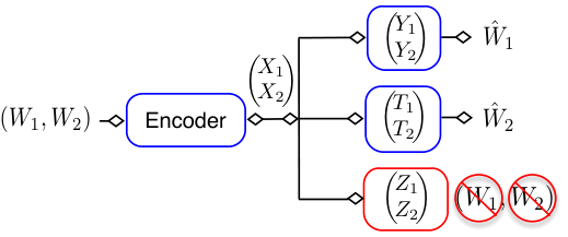
The product of inversely less-noisy broadcast channels is defined as the product of two less-noisy WBCs. The BC (Y1,T1)(Y_{1},T_{1}) has a component Y1Y_{1} which is less-noisy than T1T_{1} and an eavesdropper Z1Z_{1} is degraded towards the best user Y1Y_{1} and more-noisy than the worst user T1T_{1}. The BC (Y2,T2)(Y_{2},T_{2}) is less-noisy in the inverse order and the eavesdropper Z2Z_{2} is degraded towards T2T_{2} and more-noisy than Y2Y_{2}.

Refer to caption
Figure 6: The Parallel Broadcast Channel (PBC) with an eavesdropper.
Theorem 9 (Product of two inversely less-noisy BCs with a more-noisy eavesdropper).

The secrecy capacity region of such a setting is given by the set of rates pairs (R1,R2)(R_{1},R_{2}) satisfying:

R1\displaystyle R_{1} ≤\displaystyle\,\leq\, I⁡(X1;Y1|Z1)+I⁡(U2,Y2)−I⁡(U2,Z2),\displaystyle I(X_{1};Y_{1}|Z_{1})+I(U_{2};Y_{2})-I(U_{2};Z_{2})\ , (53)
R2\displaystyle R_{2} ≤\displaystyle\leq I⁡(X2;T2|Z2)+I⁡(U1,T1)−I⁡(U1,Z1),\displaystyle I(X_{2};T_{2}|Z_{2})+I(U_{1};T_{1})-I(U_{1};Z_{1})\ , (54)
R1+R2\displaystyle R_{1}+R_{2} ≤\displaystyle\leq I⁡(X1;Y1|Z1)+I⁡(U2,Y2)−I⁡(U2,Z2)\displaystyle I(X_{1};Y_{1}|Z_{1})+I(U_{2};Y_{2})-I(U_{2};Z_{2}) (55)
+I⁡(X2;T2|Z2​U2),\displaystyle\qquad\qquad+I(X_{2};T_{2}|Z_{2}U_{2})\ ,
R1+R2\displaystyle R_{1}+R_{2} ≤\displaystyle\leq I⁡(X2;T2|Z2)+I⁡(U1,T1)−I⁡(U1,Z1)\displaystyle I(X_{2};T_{2}|Z_{2})+I(U_{1};T_{1})-I(U_{1};Z_{1}) (56)
+I⁡(X1;Y1|Z1​U1),\displaystyle\qquad\qquad+I(X_{1};Y_{1}|Z_{1}U_{1})\ ,

for some input p.m.f PU1​X1​U2​X2=PU1​X1​PU2​X2P_{U_{1}X_{1}U_{2}X_{2}}=P_{U_{1}X_{1}}P_{U_{2}X_{2}} that satisfies (U1,U2)−⦵−(X1,X2)−⦵−(Y1,Y2,T1,T2,Z1,Z2)(U_{1},U_{2})-\!\!\!\!\minuso\!\!\!\!-(X_{1},X_{2})-\!\!\!\!\minuso\!\!\!\!-(Y_{1},Y_{2},T_{1},T_{2},Z_{1},Z_{2}).

Proof.

The proof is quite evolved in that it requires a new outer bound formulation, and is thus relegated to Appendix G. ∎

Note here that, in the absence of the eavesdropper, this theorem yields the capacity region of the product of two reversely less-noisy BCs which, though not proved in [24], can be deducted from the result of [25] for the product of reversely more-capable BCs.

IV The BEC/BSC Broadcast Channel with a BSC eavesdropper

In this section, we characterize the capacity region of the BEC/BSC broadcast channel with an external BSC eavesdropper. This model falls into the class of ordered BCs and is extremely rich since the BC (BEC and BSC) provides for a variety of orderings following the respective values of the erasure probability “ee" and the crossover probability “pp", as it is summarized in the table I and shown in [26]. Let us consider the channel model where:

𝒲:{𝒳⟼𝒴1≡BEC(e),𝒳⟼𝒴2≡BSC(p2),𝒳⟼𝒵≡BSC(p).\mathcal{W}\,:\,\left\{\begin{array}[]{lcl}{\mathcal{X}}&\longmapsto&{\mathcal{Y}}_{1}\equiv\textrm{BEC($e$)}\,,\\ {\mathcal{X}}&\longmapsto&{\mathcal{Y}}_{2}\equiv\textrm{BSC($p_{2}$)}\,,\\ {\mathcal{X}}&\longmapsto&\mathcal{Z}\,\,\equiv\textrm{BSC(p)}\,.\end{array}\right.\vskip 2.84526pt (57)
0≤e≤2​p\!\!\!0\leq e\leq 2p\!\!\! 2​p<e≤4​p​(1−p)\!\!\!2p<e\leq 4p(1-p)\!\!\! 4​p​(1−p)<e≤h⁡(p)\!\!\!4p(1-p)<e\leq h(p)\!\!\! h⁡(p)<e≤\!\!\!h(p)<e\leq 1\!\!\!
Degraded Less-noisy More-capable Es.Less-noisy
Table I: Different orderings allowed by BEC(e) and BSC(p) models.

We will consider the case where Y1Y_{1} is less-noisy that Y2Y_{2} and where ZZ is degraded towards Y2Y_{2}. Besides, we make sure that ZZ is degraded towards Y1Y_{1}. 11 1 It is worth emphasizing here that our choice of ZZ degraded respect to Y2Y_{2} follows from that both channels are naturally degraded since these are B​S​CBSC channels. Otherwise, if Y2Y_{2} were to be degraded respect to ZZ, no positive rate could be transmitted to user 22 . Summarizing these constraints, we end up with the inequalities:

2​p2≤e≤min⁡{2​p,4​p2​(1−p2)}.2p_{2}\leq e\leq\min\{2p,4p_{2}(1-p_{2})\}\ . (58)
Theorem 10 (Secrecy capacity region of the BEC(ee) /BSC(p2p_{2}) BC with BSC(pp) eavesdropper).

The capacity region of the BC with BEC(ee) / BSC(p2p_{2}) components and a BSC(pp) eavesdropper, defined by the constraint (58) where 1−4​p​(1−p)≥4​p2​(1−p2)1-4p(1-p)\geq 4p_{2}(1-p_{2}), is given by the set of rate pairs satisfying:

𝒞:{R1≤(1−e)​h2​(x)+h2​(p)−h2​(p⋆x),R2≤h2​(p⋆x)−h2​(p2⋆x),\mathcal{C}\,:\left\{\begin{array}[]{rcl}R_{1}&\leq&(1-e)\,h_{2}(x)+h_{2}(p)-h_{2}(p\star x)\ ,\\ R_{2}&\leq&h_{2}(p\star x)-h_{2}(p_{2}\star x)\ ,\end{array}\right. (59)

for some x∈[0:0.5]x\in[0:0.5].

Proof.

The proof consists in evaluating the capacity region of such an ordered channel given by ℛ\mathcal{R}, the set of rate pairs (R1,R2)(R_{1},R_{2}) satisfying:

R1≤I⁡(X;Y1|T​U)−I⁡(X;Z|T​U)=I⁡(X;Y1|Z​T​U),R2≤I⁡(U;Y2|T)−I⁡(U;Z|T)=I⁡(U;Y2|Z​T),\begin{array}[]{rcl}R_{1}&\leq&I(X;Y_{1}|TU)-I(X;Z|TU)=I(X;Y_{1}|ZTU)\ ,\\ R_{2}&\leq&I(U;Y_{2}|T)-I(U;Z|T)=I(U;Y_{2}|ZT)\ ,\end{array} (60)

and is two fold. The challenging part is obviously the converse part since it requires the use of an inequality, similar in a way to Mrs. Gerber’s lemma [20] applied to the secrecy capacity region, which we have been able to prove only under the assumption 1−4​p​(1−p)≥4​p2​(1−p2)1-4p(1-p)\geq 4p_{2}(1-p_{2}), although there is strong evidence that the converse can be proved besides this case.

Note that T=∅T=\emptyset maximizes the region since it can easily be shown to be convex and thus, will not need the time-sharing variable TT. Moreover, we can state a cardinality bound on the auxiliary rv UU used in evaluating the previous region following the usual Fenchel-Eggleston-Caratheodory theorem that is it suffices to evaluate the region using an auxiliary rv with a quaternary alphabet.

First, note that the choice X=U⊕VX=U\oplus V where U∼Bern​(0.5)U\sim\textrm{Bern}(0.5), V∼Bern​(x)V\sim\textrm{Bern}(x) yields that X∼Bern​(0.5)X\sim\textrm{Bern}(0.5) and that X|U∼Bern​(x)X|U\sim\textrm{Bern}(x). Thus, we can write:

I⁡(X;Y1|U)\displaystyle I(X;Y_{1}|U) =\displaystyle\,=\, (1−e)​H​(X|U)=(1−e)​h2​(x),\displaystyle(1-e)H(X|U)=(1-e)h_{2}(x)\ , (61)
I⁡(X;Z|U)\displaystyle I(X;Z|U) =\displaystyle= h2​(p∗x)−h2​(p),\displaystyle h_{2}(p*x)-h_{2}(p)\ , (62)
I⁡(U,Y2)\displaystyle I(U;Y_{2}) =\displaystyle= 1−h2​(p2∗x),\displaystyle 1-h_{2}(p_{2}*x)\ , (63)
I⁡(U,Z)\displaystyle I(U;Z) =\displaystyle= 1−h2​(p∗x),\displaystyle 1-h_{2}(p*x)\ , (64)

which proves the inclusion of the region ℛ\mathcal{R} in the rate region 𝒞\mathcal{C}, i.e., the achievability.

As for the inclusion in the appositive way, i.e., the converse, we will use the following lemma.

Lemma 1.

If 1−4​p​(1−p)≤4​p2​(1−p2)1-4p(1-p)\leq 4p_{2}(1-p_{2}), then ℛ\mathcal{R} defines a convex set.

Proof:

The proof is given in Appendix E. ∎

Now, since ℛ\mathcal{R} and 𝒞\mathcal{C} define convex bounded sets, then both are uniquely defined by their supporting hyperplanes. And finally, since ℛ\mathcal{R} is included in 𝒞\mathcal{C}, it thus suffices to show that all their supporting hyperplanes intersect, so let then λ∈[0:∞[\lambda\in[0:\infty[. We want to show that22 2 Note that the maxima are well defined for both regions due to the cardinality bound (for 𝒞\mathcal{C}) and for the closed and bounded interval for ℛ\mathcal{R} which results in compact supports for both optimizations.:

max(R1,R2)∈𝒞​R1+λ​R2≤max(R1,R2)∈ℛ​R1+λ​R2.\underset{(R_{1},R_{2})\in\mathcal{C}}{\max}R_{1}+\lambda R_{2}\leq\underset{(R_{1},R_{2})\in\mathcal{R}}{\max}R_{1}+\lambda R_{2}\ . (65)

Let us choose the following notation: UU is an auxiliary rv that takes its values in 𝒰={1,…,‖𝒰‖}\mathcal{U}=\{1,\dots,\|\mathcal{U}\|\} following the law: ℙ⁡(U=u)=PU​(u)≜Pu\mathds{P}(U=u)=P_{U}(u)\triangleq P_{u}. Let us assume that XX is a Bern​(α)\textrm{Bern}(\alpha) distributed Binary rv and that33 3 𝒰\mathcal{U} is the support of the law PUP_{U}, as such, PX|U​(0|u)P_{X|U}(0|u) is well defined. ℙ⁡(X=0|U=u)=PX|U​(0|u)≜xu\mathds{P}(X=0|U=u)=P_{X|U}(0|u)\triangleq x_{u}.

Define the set 𝒫\mathcal{P} of admissible transition probabilities as:

𝒫≜{(α,x‖𝒰‖,p‖𝒰‖)=(α,x1,…,x‖𝒰‖,p1,…,p‖𝒰‖)\displaystyle\mathcal{P}\triangleq\biggl\{(\alpha,\textbf{x}_{\|\mathcal{U}\|},\textbf{p}_{\|\mathcal{U}\|})=(\alpha,x_{1},\dots,x_{\|\mathcal{U}\|},p_{1},\dots,p_{\|\mathcal{U}\|})
∈[0:0.5]‖𝒰‖+1×[0:1]‖𝒰‖\displaystyle\qquad\qquad\qquad\qquad\in\left[0:0.5\right]^{\|\mathcal{U}\|+1}\times\left[0:1\right]^{\|\mathcal{U}\|}
 s.t ∑u=1‖𝒰‖pu=1,∑u=1‖𝒰‖puxu=α}.\displaystyle\qquad\qquad\text{ s.t }\sum_{u=1}^{\|\mathcal{U}\|}p_{u}=1\ ,\ \sum_{u=1}^{\|\mathcal{U}\|}p_{u}x_{u}=\alpha\biggr\}\ . (66)

With this, note that:

max(R1,R2)∈𝒞​R1+λ​R2\displaystyle\underset{(R_{1},R_{2})\in\mathcal{C}}{\max}R_{1}+\lambda R_{2} (70)
=\displaystyle= maxPU​XU−⦵−X−⦵−(Y1,Y2,Z)​I​(X;Y1|U)−I⁡(X;Z|U)\displaystyle\underset{\begin{subarray}{c}P_{UX}\\ U-\!\!\!\!\minuso\!\!\!\!-X-\!\!\!\!\minuso\!\!\!\!-(Y_{1},Y_{2},Z)\end{subarray}}{\max}I(X;Y_{1}|U)-I(X;Z|U)
+λ⁡[I⁡(U,Y2)−I⁡(U,Z)]\displaystyle\qquad\qquad\qquad+\lambda\Bigl[I(U;Y_{2})-I(U;Z)\Bigr]
=\displaystyle= max(α,x‖𝒰‖,p‖𝒰‖)∈𝒫​h2​(p)+λ⁡[h2​(p2∗α)−h2​(p∗α)]\displaystyle\underset{(\alpha\,,\,\textbf{x}_{\|\mathcal{U}\|}\,,\,\textbf{p}_{\|\mathcal{U}\|})\in\mathcal{P}}{\max}h_{2}(p)+\lambda\Bigl[h_{2}(p_{2}*\alpha)-h_{2}(p*\alpha)\Bigr]
+∑u∈𝒰Pu{(1−e)h2(xu)−h2(p∗xu)\displaystyle\quad+\sum_{u\in\mathcal{U}}P_{u}\left\{\vphantom{\Bigr]}(1-e)h_{2}(x_{u})-h_{2}(p*x_{u})\right.
+λ[h2(p∗xu)−h2(p2∗xu)]}\displaystyle\qquad\left.+\lambda\Bigl[h_{2}(p*x_{u})-h_{2}(p_{2}*x_{u})\Bigr]\right\}
≤(a)\displaystyle\overset{(a)}{\leq} max(α,x‖𝒰‖,p‖𝒰‖)∈𝒫h2​(p)\displaystyle\underset{(\alpha\,,\,\textbf{x}_{\|\mathcal{U}\|}\,,\,\textbf{p}_{\|\mathcal{U}\|})\in\mathcal{P}}{\max}\quad h_{2}(p)
+∑u∈𝒰Pu{(1−e)h2(xu)−h2(p∗xu)\displaystyle\quad+\sum_{u\in\mathcal{U}}P_{u}\left\{\vphantom{\Bigr]}(1-e)h_{2}(x_{u})-h_{2}(p*x_{u})\right.
+λ[h2(p∗xu)−h2(p2∗xu)]}\displaystyle\qquad\left.+\lambda\Bigl[h_{2}(p*x_{u})-h_{2}(p_{2}*x_{u})\Bigr]\right\}\ \ \ \
≤(b)\displaystyle\overset{(b)}{\leq} h2​(p)+(1−e)​h2​(xuλ)−h2​(p∗xuλ)\displaystyle h_{2}(p)+(1-e)h_{2}(x_{u}^{\lambda})-h_{2}(p*x_{u}^{\lambda})
+λ⁡[h2​(p∗xuλ)−h2​(p2∗xuλ)]\displaystyle\qquad+\lambda\Bigl[h_{2}(p*x_{u}^{\lambda})-h_{2}(p_{2}*x_{u}^{\lambda})\Bigr]
=\displaystyle= max(R1,R2)∈ℛ​R1+λ​R2,\displaystyle\underset{(R_{1},R_{2})\in\mathcal{R}}{\max}R_{1}+\lambda R_{2}\ , (71)

where:

xuλ\displaystyle x_{u}^{\lambda} =\displaystyle= argmax{(1−e)h2(x)−h2(p∗x)\displaystyle\arg\max\left\{\vphantom{\Bigr]}(1-e)h_{2}(x)-h_{2}(p*x)\right. (72)
+λ[h2(p∗x)−h2(p2∗x)]}.\displaystyle\qquad\left.\qquad+\lambda\Bigl[h_{2}(p*x)-h_{2}(p_{2}*x)\Bigr]\right\}\ .

Now, (a)(a) follows from the fact that since x,p1,p2∈[0:1/2]x,p_{1},p_{2}\in[0:1/2] and p≥p2p\geq p_{2}, then:

∀α∈[0:1/2],p2∗α≤p∗α≤1/2\displaystyle\forall\alpha\in[0:1/2]\quad,\quad p_{2}*\alpha\leq p*\alpha\leq 1/2 (73)
then maxα∈[0:1/2][h2(p2∗α)−h2(p∗α)]=0\displaystyle\max_{\alpha\in[0:1/2]}\left[h_{2}(p_{2}*\alpha)-h_{2}(p*\alpha)\right]=0 (74)

with equality for α=1/2\alpha=1/2. As for (b)(b), it is a direct result of the existence of a value of xuλx_{u}^{\lambda} that maximizes the expression, and from that letting 𝒰={0,1}\mathcal{U}=\{0,1\} and P0=P1=12P_{0}=P_{1}=\frac{1}{2} and U⟼X≡B​S​C​(xuλ)U\longmapsto X\equiv BSC(x_{u}^{\lambda}), leads to this maximum value equality in (b)(b) in addition to being admissible: P0​xuλ+P1​(1−xuλ)=α=12P_{0}x_{u}^{\lambda}+P_{1}(1-x_{u}^{\lambda})=\alpha=\frac{1}{2}. This ends the proof of equality of the two rate regions. ∎

In the sequel, we evaluate the effect of eavesdropping on such a BEC(ee)/BSC(p2p_{2}) BC with a BSC(pp) eavesdropper.

First note 𝒞s​t​d\mathcal{C}_{std} the standard capacity region of the BC without an eavesdropper, 𝒞\mathcal{C} being its secrecy capacity region. We have that [26]:

𝒞s​t​d:{R1≤(1−e)​h2​(x),R2≤1−h2​(p2⋆x),\mathcal{C}_{std}\,:\left\{\begin{array}[]{rcl}R_{1}&\leq&(1-e)\,h_{2}(x)\ ,\\ R_{2}&\leq&1-h_{2}(p_{2}\star x)\ ,\end{array}\right. (75)

for some x∈[0:0.5]x\in[0:0.5].

The presence of eavesdropper engenders an impediment on the sum rate given by 1−h2​(p)1-h_{2}(p), that does not depend on the choice of the channel parameters (e,p2)(e,p_{2}). As such, it turns out that the channel to user 22 ,i.e. BSC(p2p_{2}) is very sensitive to such the BSC(pp) eavesdropper in that it could have zero admissible rate R2R_{2} if the eavesdropper were to have a channel as good as to allow for p=p2p=p_{2}. However, and that’s peculiar to the BEC(ee) channel, user 11 always has strictly positive rates whatever the value of pp, since e≤2​p≤h2​(p)e\leq 2p\leq h_{2}(p) and thus, a rate of h2​(p)−2​p>0h_{2}(p)-2p>0 is always achievable.

To illustrate this, we consider the following transmission scheme where e=2​pe=2p, i.e. the worst eavesdropper is considered for user 11, and where we vary pp in the interval [p2:0.5][p_{2}:0.5]. Fig 7 plots the obtained curves. As expected, the eavesdropper has no impediment on the available rates for both users when pp is close to 0.50.5, however, as pp decreases, the gap between the standard capacity region and the secrecy capacity region increases, and the rate available at user 22 decreases to zero whilst that of user 11, stays above a given threshold.

Figure 7: Secrecy capacity region of the BC with BEC(ee)/BSC(p2p_{2}) components and a BSC(pp) eavesdropper.

V Proof of Theorem 1: Outer Bound

In this section, we prove the outer bound in Theorem 1, since this rate region is symmetric in the rates RjR_{j}, j∈{1,2}j\in\{1,2\}, the constraints will be shown only for the following two single rates and two sum-rates:

R1\displaystyle R_{1} ≤\displaystyle\leq I⁡(U1;Y1|T​V1)−I⁡(U1;Z|T​V1),\displaystyle I(U_{1};Y_{1}|TV_{1})-I(U_{1};Z|TV_{1})\ , (76)
R1\displaystyle R_{1} ≤\displaystyle\leq I⁡(U1;Y1​Y2|T​V1​V2)−I⁡(U1;Z|T​V1​V2),\displaystyle I(U_{1};Y_{1}Y_{2}|TV_{1}V_{2})-I(U_{1};Z|TV_{1}V_{2})\ , (77)
R1+R2\displaystyle R_{1}+R_{2} ≤\displaystyle\leq I⁡(X;Y2|T​Z​V1)+I⁡(U1​S1;Y1|T​V1)\displaystyle I(X;Y_{2}|TZV_{1})+I(U_{1}S_{1};Y_{1}|TV_{1}) (78)
−I⁡(U1​S1;Z​Y2|T​V1),\displaystyle\qquad\qquad-I(U_{1}S_{1};ZY_{2}|TV_{1})\ ,
R1+R2\displaystyle R_{1}+R_{2} ≤\displaystyle\leq I⁡(X;Y2|T​Z​V1​V2)+I⁡(U1​S1;Y1​Y2|T​V1​V2)\displaystyle I(X;Y_{2}|TZV_{1}V_{2})+I(U_{1}S_{1};Y_{1}Y_{2}|TV_{1}V_{2}) (79)
−I⁡(U1​S1;Z​Y2|T​V1​V2).\displaystyle\qquad\qquad-I(U_{1}S_{1};ZY_{2}|TV_{1}V_{2})\ .

V-A Single rates’ constraints

By Fano’s inequality we have that:

n​R1≤I⁡(W1,Y1n)+n​ϵn.nR_{1}\leq I(W_{1};Y_{1}^{n})+n\,\epsilon_{n}\ . (80)

Moreover, from the secrecy constraint: I⁡(W1,Zn)≤n​ϵnI(W_{1};Z^{n})\leq n\,\epsilon_{n}. Thus, one can write that:

n⁡(R1−2​ϵn)\displaystyle n(R_{1}-2\epsilon_{n}) (81)
≤\displaystyle\leq I⁡(W1,Y1n)−I⁡(W1,Zn)\displaystyle I(W_{1};Y_{1}^{n})-I(W_{1};Z^{n})
=\displaystyle= ∑i=1n[I⁡(W1;Y1,i|Y1i−1)−I⁡(W1;Zi|Zi+1n)]\displaystyle\sum^{n}_{i=1}\left[I(W_{1};Y_{1,i}|Y^{i-1}_{1})-I(W_{1};Z_{i}|Z^{n}_{i+1})\right] (82)
=(a)\displaystyle\overset{(a)}{=} ∑i=1n[I⁡(W1​Zi+1n;Y1,i|Y1i−1)−I⁡(W1​Y1i−1;Zi|Zi+1n)]\displaystyle\sum^{n}_{i=1}\left[I(W_{1}Z^{n}_{i+1};Y_{1,i}|Y^{i-1}_{1})-I(W_{1}Y^{i-1}_{1};Z_{i}|Z^{n}_{i+1})\right]\,\,\,\,\,\, (83)
=(b)\displaystyle\overset{(b)}{=} ∑i=1n[I⁡(W1;Y1,i|Y1i−1​Zi+1n)−I⁡(W1;Zi|Y1i−1​Zi+1n)]\displaystyle\sum^{n}_{i=1}\left[I(W_{1};Y_{1,i}|Y^{i-1}_{1}Z^{n}_{i+1})-I(W_{1};Z_{i}|Y^{i-1}_{1}Z^{n}_{i+1})\right]\,\,\,\,\,\, (84)

where (a)(a) and (b)(b) follow both from the Csiszár & Körner’s sum-identity (156):

∑i=1n[I⁡(Zi+1n;Y1,i|W1​Y1i−1)−I⁡(Y1i−1;Zi|W1​Zi+1n)]\displaystyle\sum^{n}_{i=1}\left[I(Z^{n}_{i+1};Y_{1,i}|W_{1}Y^{i-1}_{1})-I(Y^{i-1}_{1};Z_{i}|W_{1}Z^{n}_{i+1})\right] =\displaystyle= 0,\displaystyle 0\ ,\qquad (85)
∑i=1n[I⁡(Zi+1n;Y1,i|Y1i−1)−I⁡(Y1i−1;Zi|Zi+1n)]\displaystyle\sum^{n}_{i=1}\left[I(Z^{n}_{i+1};Y_{1,i}|Y^{i-1}_{1})-I(Y^{i-1}_{1};Z_{i}|Z^{n}_{i+1})\right] =\displaystyle= 0.\displaystyle 0\ . (86)

We then define: U1,i=W1U_{1,i}=W_{1}, V1,i=Y1i−1V_{1,i}=Y^{i-1}_{1} and Ti=Zi+1nT_{i}=Z^{n}_{i+1}, which yields the first single rate constraint.

In the same fashion, we can write the other single rates by treating the two outputs Y1Y_{1} and Y2Y_{2} together, i.e Y1∼(Y1,Y2)Y_{1}\sim(Y_{1},Y_{2}) letting V2,i=Y2i−1V_{2,i}=Y^{i-1}_{2}. We end up with the couple of constraints:

{R1≤I⁡(U1;Y1|T​V1)−I⁡(U1;Z|T​V1),R1≤I⁡(U1;Y1​Y2|T​V1​V2)−I⁡(U1;Z|T​V1​V2).\left\{\begin{array}[]{rcl}R_{1}&\leq&I(U_{1};Y_{1}|TV_{1})-I(U_{1};Z|TV_{1})\ ,\\ R_{1}&\leq&I(U_{1};Y_{1}Y_{2}|TV_{1}V_{2})-I(U_{1};Z|TV_{1}V_{2})\ .\end{array}\right. (87)

Furthermore, similar all manipulations can be performed by starting from the Fano’s inequality and secrecy requirement:

n​R1≤I⁡(W1;Y1n|W2)−I⁡(W1;Zn|W2)+n​ϵn.nR_{1}\leq I(W_{1};Y_{1}^{n}|W_{2})-I(W_{1};Z^{n}|W_{2})+n\,\epsilon_{n}\ . (88)

Thus, we could condition over U2,i=W2U_{2,i}=W_{2} the two previous rate constraints to obtain:

{R1≤I⁡(U1;Y1|T​V1​U2)−I⁡(U1;Z|T​V1​U2),R1≤I⁡(U1;Y1​Y2|T​V1​U2​V2)−I⁡(U1;Z|T​V1​U2​V2).\left\{\begin{array}[]{rcl}R_{1}&\leq&I(U_{1};Y_{1}|TV_{1}U_{2})-I(U_{1};Z|TV_{1}U_{2})\ ,\\ R_{1}&\leq&I(U_{1};Y_{1}Y_{2}|TV_{1}U_{2}V_{2})-I(U_{1};Z|TV_{1}U_{2}V_{2})\ .\end{array}\right. (89)

V-B Sum-rate constraints

Let us start by Fano’s inequality writing:

n​R1≤I⁡(W1,Y1n)−I⁡(W1,Y2n​Zn)+I⁡(W1,Y2n​Zn)+n​ϵn.n\,R_{1}\leq I(W_{1};Y_{1}^{n})-I(W_{1};Y^{n}_{2}Z^{n})+I(W_{1};Y^{n}_{2}Z^{n})+n\,\epsilon_{n}\ . (90)

Then, combining with the following constraint obtained from Fano’s inequality:

n​R2≤I⁡(W2;Y2n​Zn|W1)+n​ϵn,n\,R_{2}\leq I(W_{2};Y^{n}_{2}Z^{n}|W_{1})+n\,\epsilon_{n}\ , (91)

we can write:

n⁡(R1+R2)\displaystyle n\,(R_{1}+R_{2}) ≤\displaystyle\leq I⁡(W1,Y1n)−I⁡(W1,Y2n​Zn)\displaystyle I(W_{1};Y_{1}^{n})-I(W_{1};Y^{n}_{2}Z^{n}) (92)
+I⁡(W1​W2,Y2n​Zn)+2​n​ϵn.\displaystyle\qquad+I(W_{1}W_{2};Y^{n}_{2}Z^{n})+2n\,\epsilon_{n}\ .

Now, let us elaborate on that:

I⁡(W1,Y1n)−I⁡(W1,Y2n​Zn)\displaystyle I(W_{1};Y_{1}^{n})-I(W_{1};Y^{n}_{2}Z^{n}) (95)
=\displaystyle= ∑i=1n[I⁡(W1;Y1,i|Y1i−1)−I⁡(W1;Y2,i​Zi|Y2,i+1n​Zi+1n)]\displaystyle\sum^{n}_{i=1}\left[I(W_{1};Y_{1,i}|Y^{i-1}_{1})-I(W_{1};Y_{2,i}Z_{i}|Y^{n}_{2,i+1}Z^{n}_{i+1})\right]\qquad
=(a)\displaystyle\overset{(a)}{=} ∑i=1n[I(W1Y2,i+1nZi+1n;Y1,i|Y1i−1)\displaystyle\sum^{n}_{i=1}\bigl[I(W_{1}Y^{n}_{2,i+1}Z^{n}_{i+1};Y_{1,i}|Y^{i-1}_{1})
−I(W1Y1i−1;Y2,iZi|Y2,i+1nZi+1n)]\displaystyle\qquad\qquad-I(W_{1}Y^{i-1}_{1};Y_{2,i}Z_{i}|Y^{n}_{2,i+1}Z^{n}_{i+1})\bigr]
=\displaystyle= ∑i=1n[I(W1Y1i−1Y2,i+1nZi+1n;Y1,i)\displaystyle\sum^{n}_{i=1}\bigl[I(W_{1}Y^{i-1}_{1}Y^{n}_{2,i+1}Z^{n}_{i+1};Y_{1,i})
−I⁡(W1​Y1i−1​Y2,i+1n​Zi+1n,Y2,i​Zi)\displaystyle\qquad\qquad-I(W_{1}Y^{i-1}_{1}Y^{n}_{2,i+1}Z^{n}_{i+1};Y_{2,i}Z_{i})
+I(Y2,i+1nZi+1n;Y2,iZi)−I(Y1i−1;Y1,i)],\displaystyle\vphantom{\sum^{n}_{i=1}}\qquad\qquad+I(Y^{n}_{2,i+1}Z^{n}_{i+1};Y_{2,i}Z_{i})-I(Y^{i-1}_{1};Y_{1,i})\bigr]\ ,

where (a)(a) is again a consequence of Csiszár & Körner’s sum-identity (156):

∑i=1nI⁡(Zi+1n;Y1,i|W1​Y1i−1)\displaystyle\sum^{n}_{i=1}I(Z^{n}_{i+1};Y_{1,i}|W_{1}Y^{i-1}_{1}) (96)
=\displaystyle= ∑i=1nI⁡(Y1i−1;Y2,i​Zi|W1​Y2,i+1n​Zi+1n).\displaystyle\sum^{n}_{i=1}I(Y^{i-1}_{1};Y_{2,i}Z_{i}|W_{1}Y^{n}_{2,i+1}Z^{n}_{i+1})\ .

As for the other term, note that:

I⁡(W1​W2,Y2n​Zn)\displaystyle I(W_{1}W_{2};Y^{n}_{2}Z^{n}) =\displaystyle= ∑i=1n[I(W1W2Y2,i+1nZi+1n;Y2,iZi)\displaystyle\sum^{n}_{i=1}\bigl[I(W_{1}W_{2}Y^{n}_{2,i+1}Z^{n}_{i+1};Y_{2,i}Z_{i}) (97)
−I(Y2,i+1nZi+1n;Y2,iZi)].\displaystyle\qquad\quad-I(Y^{n}_{2,i+1}Z^{n}_{i+1};Y_{2,i}Z_{i})\bigr]\ .\,\,\,

Looking at the first term of the last equality:

∑i=1nI⁡(W1​W2​Y2,i+1n​Zi+1n,Y2,i​Zi)\displaystyle\sum^{n}_{i=1}I(W_{1}W_{2}Y^{n}_{2,i+1}Z^{n}_{i+1};Y_{2,i}Z_{i}) (101)
=\displaystyle= ∑i=1n[I(W1W2Y2,i+1nZi+1nZi−1;Y2,iZi)\displaystyle\sum^{n}_{i=1}\left[I(W_{1}W_{2}Y^{n}_{2,i+1}Z^{n}_{i+1}Z^{i-1};Y_{2,i}Z_{i})\right.
−I(Zi−1;Y2,iZi|W1W2Y2,i+1nZi+1n)]\displaystyle\qquad\left.-I(Z^{i-1};Y_{2,i}Z_{i}|W_{1}W_{2}Y^{n}_{2,i+1}Z^{n}_{i+1})\right]
=(a)\displaystyle\overset{(a)}{=} ∑i=1n[I(W1W2Y2,i+1nZi+1nZi−1;Y2,iZi)\displaystyle\sum^{n}_{i=1}\left[I(W_{1}W_{2}Y^{n}_{2,i+1}Z^{n}_{i+1}Z^{i-1};Y_{2,i}Z_{i})\right.
−I(Y2,i+1nZi+1n;Zi|W1W2Zi−1)]\displaystyle\qquad\left.-I(Y^{n}_{2,i+1}Z^{n}_{i+1};Z_{i}|W_{1}W_{2}Z^{i-1})\right]
=\displaystyle= ∑i=1n[I(W1W2Zi−1;Zi)\displaystyle\sum^{n}_{i=1}\left[I(W_{1}W_{2}Z^{i-1};Z_{i})\right.
+I(W1W2Y2,i+1nZi+1nZi−1;Y2,i|Zi)]\displaystyle\qquad\left.+I(W_{1}W_{2}Y^{n}_{2,i+1}Z^{n}_{i+1}Z^{i-1};Y_{2,i}|Z_{i})\right]
=\displaystyle= ∑i=1n[I(W1W2;Zi|Zi−1)+I(Zi−1;Zi)\displaystyle\sum^{n}_{i=1}\left[I(W_{1}W_{2};Z_{i}|Z^{i-1})+I(Z^{i-1};Z_{i})\right.
+I(W1W2Y2,i+1nZi+1nZi−1;Y2,i|Zi)].\displaystyle\qquad\left.+I(W_{1}W_{2}Y^{n}_{2,i+1}Z^{n}_{i+1}Z^{i-1};Y_{2,i}|Z_{i})\right]\ .

Here, (a)(a) is a consequence of Csiszár & Körner’s sum-identity (156) but between the outputs ZZ and (Y2,Z)(Y_{2},Z):

∑i=1nI⁡(Zi−1;Y2,i​Zi|W1​W2​Y2,i+1n​Zi+1n)\displaystyle\sum^{n}_{i=1}I(Z^{i-1};Y_{2,i}Z_{i}|W_{1}W_{2}Y^{n}_{2,i+1}Z^{n}_{i+1}) (102)
=\displaystyle= ∑i=1nI⁡(Y2,i+1n​Zi+1n;Zi|W1​W2​Zi−1).\displaystyle\sum^{n}_{i=1}I(Y^{n}_{2,i+1}Z^{n}_{i+1};Z_{i}|W_{1}W_{2}Z^{i-1})\ .

Using the secrecy constraint, one can then notice that:

∑i=1nI⁡(W1​W2;Zi|Zi−1)=I⁡(W1​W2,Zn)≤n​ϵn.\sum^{n}_{i=1}I(W_{1}W_{2};Z_{i}|Z^{i-1})=I(W_{1}W_{2};Z^{n})\leq n\,\epsilon_{n}\ . (103)

Moreover, observe that:

∑i=1nI⁡(Zi−1,Zi)=∑i=1nI⁡(Zi+1n,Zi),\sum^{n}_{i=1}I(Z^{i-1};Z_{i})=\sum^{n}_{i=1}I(Z^{n}_{i+1};Z_{i})\ , (104)

and

I⁡(W1​W2​Y2,i+1n​Zi+1n​Zi−1;Y2,i|Zi)\displaystyle I(W_{1}W_{2}Y^{n}_{2,i+1}Z^{n}_{i+1}Z^{i-1};Y_{2,i}|Z_{i}) (105)
≤\displaystyle\leq I⁡(W1​W2​Y2,i+1n​Zi+1n​Y1i−1​Zi−1;Y2,i|Zi).\displaystyle I(W_{1}W_{2}Y^{n}_{2,i+1}Z^{n}_{i+1}Y_{1}^{i-1}Z^{i-1};Y_{2,i}|Z_{i})\ .

The sum-rate can be then bounded as follows:

n⁡(R1+R2−2​ϵn)\displaystyle n(R_{1}+R_{2}-2\epsilon_{n}) (107)
≤\displaystyle\leq I⁡(W1,Y1n)−I⁡(W1,Y2n​Zn)+I⁡(W1​W2,Y2n​Zn)\displaystyle\vphantom{\sum^{n}}I(W_{1};Y_{1}^{n})-I(W_{1};Y^{n}_{2}Z^{n})+I(W_{1}W_{2};Y^{n}_{2}Z^{n})\,\,\,
≤\displaystyle\leq ∑i=1n[I(W1Y1i−1Y2,i+1nZi+1n;Y1,i)\displaystyle\sum^{n}_{i=1}\left[I(W_{1}Y^{i-1}_{1}Y^{n}_{2,i+1}Z^{n}_{i+1};Y_{1,i})\right.
−I⁡(W1​Y1i−1​Y2,i+1n​Zi+1n,Y2,i​Zi)\displaystyle\qquad\vphantom{\sum_{i=1}}\left.-I(W_{1}Y^{i-1}_{1}Y^{n}_{2,i+1}Z^{n}_{i+1};Y_{2,i}Z_{i})\right.
+I⁡(W1​W2​Y2,i+1n​Zi+1n​Y1i−1​Zi−1;Y2,i|Zi)\displaystyle\vphantom{\sum_{i=1}}\qquad+I(W_{1}W_{2}Y^{n}_{2,i+1}Z^{n}_{i+1}Y_{1}^{i-1}Z^{i-1};Y_{2,i}|Z_{i})
+I(Zi+1n;Zi)−I(Y1i−1;Y1,i)].\displaystyle\vphantom{\sum_{i=1}}\qquad+\left.I(Z^{n}_{i+1};Z_{i})-I(Y^{i-1}_{1};Y_{1,i})\right]\ .

And to end, we use the following remarks:

∑i=1n[I⁡(Zi+1n,Zi)−I⁡(Y1i−1,Y1,i)]\displaystyle\sum^{n}_{i=1}\left[I(Z^{n}_{i+1};Z_{i})-I(Y^{i-1}_{1};Y_{1,i})\right] (109)
=\displaystyle= ∑i=1n[I⁡(Y1i−1​Zi+1n,Zi)−I⁡(Y1i−1​Zi+1n,Y1,i)]\displaystyle\sum^{n}_{i=1}\left[I(Y^{i-1}_{1}Z^{n}_{i+1};Z_{i})-I(Y^{i-1}_{1}Z^{n}_{i+1};Y_{1,i})\right]
=\displaystyle= ∑i=1n[I(Y1i−1Zi+1n;Y2,iZi)−I(Y1i−1Zi+1n;Y1,i)\displaystyle\sum^{n}_{i=1}\left[I(Y^{i-1}_{1}Z^{n}_{i+1};Y_{2,i}Z_{i})-I(Y^{i-1}_{1}Z^{n}_{i+1};Y_{1,i})\right.
−I(Y1i−1Zi+1n;Y2,i|Zi)].\displaystyle\quad\quad\left.-I(Y^{i-1}_{1}Z^{n}_{i+1};Y_{2,i}|Z_{i})\right]\ .

Thus, combining with the previous equality, we end up with:

n⁡(R1+R2−2​ϵn)\displaystyle n(R_{1}+R_{2}-2\epsilon_{n}) (112)
≤\displaystyle\leq I⁡(W1,Y1n)−I⁡(W1,Y2n​Zn)+I⁡(W1​W2,Y2n​Zn)\displaystyle\vphantom{\sum^{n}}I(W_{1};Y_{1}^{n})-I(W_{1};Y^{n}_{2}Z^{n})+I(W_{1}W_{2};Y^{n}_{2}Z^{n})
≤\displaystyle\leq ∑i=1n[I(W1Y1i−1Y2,i+1nZi+1n;Y1,i)−I(Y1i−1Zi+1n;Y1,i)\displaystyle\sum^{n}_{i=1}\left[I(W_{1}Y^{i-1}_{1}Y^{n}_{2,i+1}Z^{n}_{i+1};Y_{1,i})-I(Y^{i-1}_{1}Z^{n}_{i+1};Y_{1,i})\right.
−I⁡(W1​Y1i−1​Y2,i+1n​Zi+1n,Y2,i​Zi)+I⁡(Y1i−1​Zi+1n,Y2,i​Zi)\displaystyle\quad\vphantom{\sum_{i=1}}\left.-I(W_{1}Y^{i-1}_{1}Y^{n}_{2,i+1}Z^{n}_{i+1};Y_{2,i}Z_{i})+I(Y^{i-1}_{1}Z^{n}_{i+1};Y_{2,i}Z_{i})\right.
+I⁡(W1​W2​Y2,i+1n​Y1i−1​Zi+1n​Zi−1;Y2,i|Zi)\displaystyle\quad\vphantom{\sum_{i=1}}+\left.I(W_{1}W_{2}Y^{n}_{2,i+1}Y_{1}^{i-1}Z^{n}_{i+1}Z^{i-1};Y_{2,i}|Z_{i})\right.
−I(Y1i−1Zi+1n;Y2,i|Zi)]\displaystyle\quad\vphantom{\sum_{i=1}}\left.-I(Y^{i-1}_{1}Z^{n}_{i+1};Y_{2,i}|Z_{i})\right]
≤(a)\displaystyle\overset{(a)}{\leq} ∑i=1n[I(W1Y2,i+1n;Y1,i|Y1i−1Zi+1n)\displaystyle\sum^{n}_{i=1}\left[I(W_{1}Y^{n}_{2,i+1};Y_{1,i}|Y^{i-1}_{1}Z^{n}_{i+1})\right.
−I⁡(W1​Y2,i+1n;Y2,i​Zi|Y1i−1​Zi+1n)\displaystyle\quad\left.\vphantom{\sum_{i=1}}-I(W_{1}Y^{n}_{2,i+1};Y_{2,i}Z_{i}|Y^{i-1}_{1}Z^{n}_{i+1})\right.
+I(Xi;Y2,i|ZiY1i−1Zi+1n)]+2nϵn,\displaystyle\quad\vphantom{\sum_{i=1}}+\left.I(X_{i};Y_{2,i}|Z_{i}Y_{1}^{i-1}Z^{n}_{i+1})\right]+2n\,\epsilon_{n}\ ,

where (a)(a) is a consequence of introducing the input XiX_{i}:

I⁡(W1​W2​Y2,i+1n​Zi−1;Y2,i|Zi​Y1i−1​Zi+1n)\displaystyle I(W_{1}W_{2}Y^{n}_{2,i+1}Z^{i-1};Y_{2,i}|Z_{i}Y_{1}^{i-1}Z^{n}_{i+1}) (113)
≤\displaystyle\leq I⁡(Xi;Y2,i|Zi​Y1i−1​Zi+1n).\displaystyle I(X_{i};Y_{2,i}|Z_{i}Y_{1}^{i-1}Z^{n}_{i+1})\ .

Letting: S1,i=Y2,i+1nS_{1,i}=Y^{n}_{2,i+1}, U1,i=W1U_{1,i}=W_{1}, V1,i=Y1i−1V_{1,i}=Y^{i-1}_{1}, and Ti=Zi+1nT_{i}=Z^{n}_{i+1}, and noting that: by resorting to a standard time-sharing argument we end up with the following single-letter constraint:

R1+R2\displaystyle R_{1}+R_{2} ≤\displaystyle\leq I⁡(U1​S1;Y1|V1​T)−I⁡(U1​S1;Y2​Z|V1​T)\displaystyle I(U_{1}S_{1};Y_{1}|V_{1}T)-I(U_{1}S_{1};Y_{2}Z|V_{1}T) (114)
+I⁡(Xi;Y2|Z​V1​T).\displaystyle\qquad+I(X_{i};Y_{2}|ZV_{1}T)\ .

Similarly, we can show the same sum-rate constraint, by replacing the output Y1Y_{1} with the two outputs (Y1​Y2)(Y_{1}Y_{2}), which results in:

R1+R2\displaystyle R_{1}+R_{2} ≤\displaystyle\leq I⁡(X;Y2|T​Z​V1​V2)+I⁡(U1​S1;Y1​Y2|T​V1​V2)\displaystyle I(X;Y_{2}|TZV_{1}V_{2})+I(U_{1}S_{1};Y_{1}Y_{2}|TV_{1}V_{2}) (115)
−I⁡(U1​S1;Z​Y2|T​V1​V2).\displaystyle\qquad-I(U_{1}S_{1};ZY_{2}|TV_{1}V_{2})\ .

V-C Proof of Corollary 1

In the previous section, we found that an outer bound on the secrecy region for the Wiretap BC can be obtained by considering only the constraints:

R1\displaystyle R_{1} ≤\displaystyle\leq I⁡(U1;Y1|T​V1)−I⁡(U1;Z|T​V1),\displaystyle I(U_{1};Y_{1}|TV_{1})-I(U_{1};Z|TV_{1})\ , (116)
R2\displaystyle R_{2} ≤\displaystyle\leq I⁡(U2;Y2|T​V2)−I⁡(U2;Z|T​V2),\displaystyle I(U_{2};Y_{2}|TV_{2})-I(U_{2};Z|TV_{2})\ , (117)
R1+R2\displaystyle R_{1}+R_{2} ≤\displaystyle\leq I⁡(X;Y2|T​Z​V1)+I⁡(U1​S1;Y1|T​V1)\displaystyle I(X;Y_{2}|TZV_{1})+I(U_{1}S_{1};Y_{1}|TV_{1}) (118)
−I⁡(U1​S1;Z​Y2|T​V1),\displaystyle\quad-I(U_{1}S_{1};ZY_{2}|TV_{1})\ ,
R1+R2\displaystyle R_{1}+R_{2} ≤\displaystyle\leq I⁡(X;Y1|T​Z​V2)+I⁡(U2​S2;Y2|T​V2)\displaystyle I(X;Y_{1}|TZV_{2})+I(U_{2}S_{2};Y_{2}|TV_{2}) (119)
−I⁡(U2​S2;Z​Y1|T​V2).\displaystyle\quad-I(U_{2}S_{2};ZY_{1}|TV_{2})\ .

An important claim is then that the auxiliary rvs S1S_{1} and S2S_{2} can be eliminated with no impediment to the rate region. Since the region is symmetric in R1R_{1} and R2R_{2}, we only show the claim for S1S_{1}. We are looking for a random variable U1⋆U_{1}^{\star} such that we can write:

R1\displaystyle R_{1} ≤\displaystyle\leq I⁡(U1⋆;Y1|T​V1)−I⁡(U1⋆;Z|T​V1),\displaystyle I(U_{1}^{\star};Y_{1}|TV_{1})-I(U_{1}^{\star};Z|TV_{1})\ , (120)
R1+R2\displaystyle R_{1}+R_{2} ≤\displaystyle\leq I⁡(X;Y2|T​Z​V1)+I⁡(U1⋆;Y1|T​V1)\displaystyle I(X;Y_{2}|TZV_{1})+I(U_{1}^{\star};Y_{1}|TV_{1}) (121)
−I⁡(U1⋆;Z​Y2|T​V1).\displaystyle\quad-I(U_{1}^{\star};ZY_{2}|TV_{1})\ .

To see this, define the two following functions:

f1​(Q)\displaystyle f_{1}(Q) ≜\displaystyle\triangleq I⁡(U1;Y1|T​V1)−I⁡(U1;Z|T​V1)\displaystyle I(U_{1};Y_{1}|TV_{1})-I(U_{1};Z|TV_{1})
−I⁡(Q;Y1|T​V1)+I⁡(Q;Z|T​V1),\displaystyle\qquad-I(Q;Y_{1}|TV_{1})+I(Q;Z|TV_{1})\ ,
f2​(Q)\displaystyle f_{2}(Q) ≜\displaystyle\triangleq I⁡(U1​S1;Y1|T​V1)−I⁡(U1​S1;Y2​Z|T​V1)\displaystyle I(U_{1}S_{1};Y_{1}|TV_{1})-I(U_{1}S_{1};Y_{2}Z|TV_{1})
−I⁡(Q;Y1|T​V1)+I⁡(Q;Y2​Z|T​V1).\displaystyle\qquad-I(Q;Y_{1}|TV_{1})+I(Q;Y_{2}Z|TV_{1})\ .

We note first that:

f1​(U1)=0,f2​(U1​S1)=0.f_{1}(U_{1})=0\quad,\quad f_{2}(U_{1}S_{1})=0\ . (122)

Moreover,

f1​(U1​S1)\displaystyle f_{1}(U_{1}S_{1}) +\displaystyle+ f2​(U1)\displaystyle f_{2}(U_{1}) (123)
=\displaystyle= −I⁡(U1​S1;Y2|T​Z​V1)+I⁡(U1;Y2|T​Z​V1)\displaystyle-I(U_{1}S_{1};Y_{2}|TZV_{1})+I(U_{1};Y_{2}|TZV_{1})\,\,\,\,\,\,
=\displaystyle= −I⁡(S1;Y2|T​Z​U1​V1)\displaystyle-I(S_{1};Y_{2}|TZU_{1}V_{1}) (124)
≤\displaystyle\leq 0.\displaystyle 0\ . (125)

Therefore, either f1​(U1​S1)≤0f_{1}(U_{1}S_{1})\leq 0 and thus, letting U1⋆=(U1​S1)U_{1}^{\star}=(U_{1}S_{1}) will not reduce the region, or f2​(U1)≤0f_{2}(U_{1})\leq 0 and in this case U1⋆=UU_{1}^{\star}=U allows us to prove our claim. The same holds for the other couple of constraints on R2R_{2} and R1+R2R_{1}+R_{2}.

VI Proof of Theorem 2: Inner Bound

In this section, we prove the achievability of the inner bound stated in Theorem 2. Let R1R_{1} and R2R_{2} denote the information rates. Let TT be any the time sharing random variable. The coding argument is as follows.

VI-A Code generation, encoding and decoding procedures

VI-A1 Rate splitting

We split the message intended to each user of rate RjR_{j} into two sub-messages: one of rate R¯j=Rj−R0​j\bar{R}_{j}=R_{j}-R_{0j} that will be decoded only by the user, and one of rate R0​jR_{0j} that will be carried through the common message. Thus in stead of transmitting the message pair (w1,w2)(w_{1},w_{2}), we transmit the triple (w¯0,w¯1,w¯2)(\bar{w}_{0},\bar{w}_{1},\bar{w}_{2}).

{R¯0≜R01+R02,R¯j≜Rj−R0​j≥0.\left\{\begin{array}[]{rcl}\bar{R}_{0}&\triangleq&R_{01}+R_{02}\ ,\\ \bar{R}_{j}&\triangleq&R_{j}-R_{0j}\geq 0\ .\end{array}\right. (126)

VI-A2 Codebook generation

Generate 2n​T02^{nT_{0}} sequences qn​(s0)q^{n}(s_{0}) following

PQn​(qn​(s0))=∏i=1nPQ​(qin​(s0)),P_{Q}^{n}(q^{n}(s_{0}))=\prod_{i=1}^{n}P_{Q}(q^{n}_{i}(s_{0}))\ , (127)

where T0≥R¯0T_{0}\geq\bar{R}_{0} and map these in 2n​R¯02^{n\bar{R}_{0}} bins indexed by w¯0\bar{w}_{0}: ℬ0n​(w¯0)\mathcal{B}^{n}_{0}(\bar{w}_{0}).

For each s0∈[1:2n​T0]s_{0}\in[1:2^{nT_{0}}] and for each j∈{1,2}j\in\{1,2\}, generate 2n​Tj2^{nT_{j}} sequences ujn​(s0,sj)u_{j}^{n}(s_{0},s_{j}) following

PUj|Qn​(ujn​(s0,sj)|qn​(s0))=∏i=1nPUj|Q​(uj,in​(s0,sj)|qin​(s0)).P_{U_{j}|Q}^{n}(u_{j}^{n}(s_{0},s_{j})|q^{n}(s_{0}))=\prod_{i=1}^{n}P_{U_{j}|Q}(u_{j,i}^{n}(s_{0},s_{j})|q^{n}_{i}(s_{0}))\ . (128)

Map these sequences in 2n​R¯j2^{n\bar{R}_{j}} bins indexed by w¯j\bar{w}_{j}: ℬjn​(s0,w¯j)\mathcal{B}^{n}_{j}(s_{0},\bar{w}_{j}) and consisting in 2n⁡(Tj−R¯j)2^{n(T_{j}-\bar{R}_{j})} n-sequences. Each of these bins are divided into 2n​R~j2^{n\tilde{R}_{j}} sub-bins indexed by ljl_{j}: ℬjn​(s0,w¯j,lj)\mathcal{B}^{n}_{j}(s_{0},\bar{w}_{j},l_{j}), thus each bin contains 2n⁡(Tj−R¯j−R~j)2^{n(T_{j}-\bar{R}_{j}-\tilde{R}_{j})} sequences where 0≤R~j≤Tj−R¯j0\leq\tilde{R}_{j}\leq T_{j}-\bar{R}_{j}.

The codebook consisting of all the bins is known to all terminals, including the eavesdropper.

Figure 8: Codebook generation and encoding.

VI-A3 Encoding

Fig. 8 plots the encoding operation. To send (W¯0,W¯1,W¯2)(\bar{W}_{0},\bar{W}_{1},\bar{W}_{2}), the encoder selects at random an index s0s_{0} such that qn​(s0)∈ℬ0n​(w¯0)q^{n}(s_{0})\in\mathcal{B}^{n}_{0}(\bar{w}_{0}). Then, in the product bin ℬ1n​(s0,w¯1)×ℬ2n​(s0,w¯2)\mathcal{B}^{n}_{1}(s_{0},\bar{w}_{1})\times\mathcal{B}^{n}_{2}(s_{0},\bar{w}_{2}), it chooses at random a pair of sub-bins ℬjn​(s0,w¯1,l1)\mathcal{B}^{n}_{j}(s_{0},\bar{w}_{1},l_{1}) and ℬ2n​(s0,w¯2,l2)\mathcal{B}^{n}_{2}(s_{0},\bar{w}_{2},l_{2}) indexed by l1l_{1} and l2l_{2}. In the corresponding product sub-bin, it looks for a pair of sequences indexed with s1s_{1} and s2s_{2} satisfying:

(qn​(s0),u1n​(s0,s1),u2n​(s0,s2))∈Tδn​(Q​U1​U2).\left(q^{n}(s_{0}),u_{1}^{n}(s_{0},s_{1}),u_{2}^{n}(s_{0},s_{2})\right)\in T_{\delta}^{n}(QU_{1}U_{2})\ . (129)

Based on the Mutual Covering Lemma [27], the encoding will succeed if the following inequalities hold:

{T1−(R¯1+R~1)+T2−(R¯2+R~2)>I⁡(U1;U2|Q),0≤R~1≤T1−R¯1,0≤R~2≤T2−R¯2.\left\{\begin{array}[]{rcl}T_{1}-(\bar{R}_{1}+\tilde{R}_{1})+T_{2}-(\bar{R}_{2}+\tilde{R}_{2})&>&I(U_{1};U_{2}|Q)\ ,\\ 0&\leq&\tilde{R}_{1}\leq T_{1}-\bar{R}_{1}\ ,\\ 0&\leq&\tilde{R}_{2}\leq T_{2}-\bar{R}_{2}\ .\end{array}\right. (130)

VI-A4 Decoding

Upon receiving yjny_{j}^{n}, decoder jj looks jointly for a pair of indices (s0,sj)(s_{0},s_{j}) such that:

(qn​(s0),ujn​(s0,sj),yjn)∈Tδn​(Q​Uj​Yj).\left(q^{n}(s_{0}),u_{j}^{n}(s_{0},s_{j}),y^{n}_{j}\right)\in T_{\delta}^{n}(QU_{j}Y_{j})\ . (131)

From the decoded indices s0s_{0} and sjs_{j}, it can infer the initial values of both W¯0\bar{W}_{0} and W¯j\bar{W}_{j}.

Based on Lemma 5, the error probability can be made arbitrarily small provided that:

{Tj≤I⁡(Uj;Yj|Q),Tj+T0≤I⁡(Q​Uj,Yj).\left\{\begin{array}[]{rcl}T_{j}&\leq&I(U_{j};Y_{j}|Q)\ ,\\ T_{j}+T_{0}&\leq&I(QU_{j};Y_{j})\ .\end{array}\right. (132)

VI-B Equivocation analysis

We find conditions on the rates T0,T1,T2T_{0},T_{1},T_{2} and R~1,R~2\tilde{R}_{1},\tilde{R}_{2} to achieve perfect secrecy for all message triples (W¯0,W¯1,W¯2)(\bar{W}_{0},\bar{W}_{1},\bar{W}_{2}).

To this end, we first note that it suffices to find conditions for which 1n​I​(W¯0​W¯1​W¯2;Zn|𝒞)\frac{1}{n}I(\bar{W}_{0}\bar{W}_{1}\bar{W}_{2};Z^{n}|\mathcal{C}) can be made arbitrarily small where 𝒞\mathcal{C} denotes the codebook used in the transmission, the latter constraint leading to the individual secrecy requirements being fulfilled.

Note that:

I⁡(W¯0​W¯1​W¯2;Zn|𝒞)\displaystyle I(\bar{W}_{0}\bar{W}_{1}\bar{W}_{2};Z^{n}|\mathcal{C}) (133)
=\displaystyle= n⁡(R¯0+R¯1+R¯2)−H⁡(W¯0​W¯1​W¯2|Zn,𝒞)\displaystyle n(\bar{R}_{0}+\bar{R}_{1}+\bar{R}_{2})-H(\bar{W}_{0}\bar{W}_{1}\bar{W}_{2}|Z^{n},\mathcal{C})
=(a)\displaystyle\overset{(a)}{=} n⁡(R¯0+R¯1+R¯2)−H⁡(S0​S1​S2|Zn,𝒞)\displaystyle n(\bar{R}_{0}+\bar{R}_{1}+\bar{R}_{2})-H(S_{0}S_{1}S_{2}|Z^{n},\mathcal{C})
+H⁡(S0​S1​S2|Zn​W¯0​W¯1​W¯2,𝒞),\displaystyle\qquad\qquad+H(S_{0}S_{1}S_{2}|Z^{n}\bar{W}_{0}\bar{W}_{1}\bar{W}_{2},\mathcal{C})\ , (134)

where (a) follows from that, knowing the codebook, the sent messages are deterministic functions of the binning indices chosen.

We first start by giving a lower bound to H⁡(S0​S1​S2|Zn,𝒞)H(S_{0}S_{1}S_{2}|Z^{n},\mathcal{C}). Let us write:

H⁡(S0​S1​S2|Zn,𝒞)\displaystyle H(S_{0}S_{1}S_{2}|Z^{n},\mathcal{C}) (139)
=\displaystyle= H⁡(S0|Zn,𝒞)+H⁡(S1​S2|Zn,S0,𝒞)\displaystyle H(S_{0}|Z^{n},\mathcal{C})+H(S_{1}S_{2}|Z^{n},S_{0},\mathcal{C})
=\displaystyle= H⁡(S0|𝒞)−I⁡(S0;Zn|𝒞)+H⁡(S1​S2|S0,𝒞)\displaystyle H(S_{0}|\mathcal{C})-I(S_{0};Z^{n}|\mathcal{C})+H(S_{1}S_{2}|S_{0},\mathcal{C})
−I(S1S2;Zn|S0,𝒞)\displaystyle\quad-I(S_{1}S_{2};Z^{n}|S_{0},\mathcal{C})
=\displaystyle= n​T0−I⁡(S0;Zn|𝒞)+H⁡(S1​S2|S0,𝒞)\displaystyle nT_{0}-I(S_{0};Z^{n}|\mathcal{C})+H(S_{1}S_{2}|S_{0},\mathcal{C})
−I(S1S2;Zn|S0,𝒞)\displaystyle\quad-I(S_{1}S_{2};Z^{n}|S_{0},\mathcal{C})
=\displaystyle= n⁡(T0+T1+T2)−I⁡(S0;Zn|𝒞)\displaystyle n(T_{0}+T_{1}+T_{2})-I(S_{0};Z^{n}|\mathcal{C})
−I(S1;S2|S0,𝒞)−I(S1S2;Zn|S0,𝒞)\displaystyle\quad-I(S_{1};S_{2}|S_{0},\mathcal{C})-I(S_{1}S_{2};Z^{n}|S_{0},\mathcal{C})
=(a)\displaystyle\overset{(a)}{=} n⁡(T0+T1+T2)−I⁡(Qn;Zn|𝒞)\displaystyle n(T_{0}+T_{1}+T_{2})-I(Q^{n};Z^{n}|\mathcal{C})
−I(U1n;U2n|Qn,𝒞)−I(U1nU2n;Zn|Qn,𝒞),\displaystyle\quad-I(U_{1}^{n};U_{2}^{n}|Q^{n},\mathcal{C})-I(U_{1}^{n}U_{2}^{n};Z^{n}|Q^{n},\mathcal{C})\ ,

where (a) follows similarly from the fact that, knowing the codebook, the sent sequences are functions of the chosen binning indices.

The next lemma provides the main result for carrying on with the analysis.

Lemma 2.

Assuming the codebook generation presented before, the next inequalities hold true:

I⁡(Qn;Zn|𝒞)\displaystyle I(Q^{n};Z^{n}|\mathcal{C}) ≤\displaystyle\leq n​I​(Q,Z)+n​ϵn,\displaystyle nI(Q;Z)+n\,\epsilon_{n}\ , (140)
I(U1n;U2n|Qn,𝒞)\displaystyle I(U_{1}^{n};U_{2}^{n}|Q^{n},\mathcal{C}) ≤\displaystyle\leq n​I​(U1;U2|Q)+n​ϵn,\displaystyle nI(U_{1};U_{2}|Q)+n\,\epsilon_{n}\ , (141)
I(U1nU2n;Zn|Qn,𝒞)\displaystyle I(U_{1}^{n}U_{2}^{n};Z^{n}|Q^{n},\mathcal{C}) ≤\displaystyle\leq n​I​(U1​U2;Z|Q)+n​ϵn.\displaystyle nI(U_{1}U_{2};Z|Q)+n\,\epsilon_{n}\ . (142)
Proof:

The proof of this lemma is presented in Appendix B. ∎Lemma 2 allows us thus to write:

1n​H​(S0​S1​S2|Zn,𝒞)\displaystyle\dfrac{1}{n}H(S_{0}S_{1}S_{2}|Z^{n},\mathcal{C}) ≥\displaystyle\geq T0+T1+T2−I⁡(Q​U1​U2,Z)\displaystyle T_{0}+T_{1}+T_{2}-I(QU_{1}U_{2};Z) (143)
−I⁡(U1;U2|Q).\displaystyle-I(U_{1};U_{2}|Q)\ .

Now, let us upper bound the remainder term to be studied: H⁡(S0​S1​S2|Zn​W¯0​W¯1​W¯2,𝒞)H(S_{0}S_{1}S_{2}|Z^{n}\bar{W}_{0}\bar{W}_{1}\bar{W}_{2},\mathcal{C}).

The following Lemma is useful to carry on with the proof.

Lemma 3.

Assuming the same coding scheme presented before, then

lim supn→∞1n​H​(S0​S1​S2|Zn​W¯0​W¯1​W¯2,𝒞)\displaystyle\limsup_{n\rightarrow\infty}\dfrac{1}{n}H(S_{0}S_{1}S_{2}|Z^{n}\bar{W}_{0}\bar{W}_{1}\bar{W}_{2},\mathcal{C})
≤max⁡{0,I1,I2,I3,I4},\displaystyle\qquad\leq\max\left\{0,I_{1},I_{2},I_{3},I_{4}\right\}\ , (144)

where

I1\displaystyle I_{1} =\displaystyle= T1−R¯1−I⁡(U1;Z​U2|Q),\displaystyle T_{1}-\bar{R}_{1}-I(U_{1};ZU_{2}|Q)\ , (145)
I2\displaystyle I_{2} =\displaystyle= T2−R¯2−I⁡(U2;Z​U1|Q),\displaystyle T_{2}-\bar{R}_{2}-I(U_{2};ZU_{1}|Q)\ , (146)
I3\displaystyle I_{3} =\displaystyle= T1−R¯1+T2−R¯2\displaystyle T_{1}-\bar{R}_{1}+T_{2}-\bar{R}_{2} (147)
−I⁡(U1​U2;Z|Q)−I⁡(U1;U2|Q),\displaystyle\qquad-I(U_{1}U_{2};Z|Q)-I(U_{1};U_{2}|Q)\ ,
I4\displaystyle I_{4} =\displaystyle= T0−R¯0+T1−R¯1+T2−R¯2\displaystyle T_{0}-\bar{R}_{0}+T_{1}-\bar{R}_{1}+T_{2}-\bar{R}_{2} (148)
−I⁡(Q​U1​U2,Z)−I⁡(U1;U2|Q).\displaystyle\qquad-I(QU_{1}U_{2};Z)-I(U_{1};U_{2}|Q)\ .
Proof:

This Lemma is proved in Appendix C.∎

As a conclusion of this lemma, and combining (134) and (143) we can conclude that:

1n​I​(W¯0​W¯1​W¯2;Zn|𝒞)−ϵn\displaystyle\dfrac{1}{n}I(\bar{W}_{0}\bar{W}_{1}\bar{W}_{2};Z^{n}|\mathcal{C})-\epsilon_{n} (150)
≤\displaystyle\leq R¯0+R¯1+R¯2−(T0+T1+T2)+I⁡(Q​U1​U2,Z)\displaystyle\bar{R}_{0}+\bar{R}_{1}+\bar{R}_{2}-(T_{0}+T_{1}+T_{2})+I(QU_{1}U_{2};Z)
+I⁡(U1;U2|Q)​max⁡{0,I1,I2,I3,I4}\displaystyle\quad+I(U_{1};U_{2}|Q)\max\left\{0,I_{1},I_{2},I_{3},I_{4}\right\}
=\displaystyle= max{R¯0+R¯1+R¯2−(T0+T1+T2)\displaystyle\max\big\{\bar{R}_{0}+\bar{R}_{1}+\bar{R}_{2}-(T_{0}+T_{1}+T_{2})
+I⁡(Q​U1​U2,Z)+I⁡(U1;U2|Q),\displaystyle\qquad\qquad+I(QU_{1}U_{2};Z)+I(U_{1};U_{2}|Q)\ ,
R¯0−T0+R¯2−T2+I⁡(Q​U2,Z),\displaystyle\qquad\bar{R}_{0}-T_{0}+\bar{R}_{2}-T_{2}+I(QU_{2};Z)\ ,
R¯0−T0+R¯1−T1+I⁡(Q​U1,Z),\displaystyle\qquad\bar{R}_{0}-T_{0}+\bar{R}_{1}-T_{1}+I(QU_{1};Z)\ ,
R¯0−T0+I(Q;Z), 0}.\displaystyle\qquad\bar{R}_{0}-T_{0}+I(Q;Z)\ ,\ 0\big\}\ .

Hence, full secrecy is guaranteed by forcing all operands in the max term to be less than zero.

By collecting all inequalities and applying FME on the rates R01R_{01} and R02R_{02} (see details in Appendix D), we obtain the desired rate region:

R1\displaystyle R_{1} ≤\displaystyle\leq I⁡(Q​U1,Y1)−I⁡(Q​U1,Z),\displaystyle I(QU_{1};Y_{1})-I(QU_{1};Z)\ , (151)
R2\displaystyle R_{2} ≤\displaystyle\leq I⁡(Q​U2,Y2)−I⁡(Q​U2,Z),\displaystyle I(QU_{2};Y_{2})-I(QU_{2};Z)\ , (152)
R1+R2\displaystyle R_{1}+R_{2} ≤\displaystyle\leq I⁡(U1;Y1|Q)+I⁡(Q​U2,Y2)\displaystyle I(U_{1};Y_{1}|Q)+I(QU_{2};Y_{2}) (153)
−I⁡(Q​U1​U2,Z)−I⁡(U1;U2|Q),\displaystyle\qquad-I(QU_{1}U_{2};Z)-I(U_{1};U_{2}|Q)\ ,
R1+R2\displaystyle R_{1}+R_{2} ≤\displaystyle\leq I⁡(U2;Y2|Q)+I⁡(Q​U1,Y1)\displaystyle I(U_{2};Y_{2}|Q)+I(QU_{1};Y_{1}) (154)
−I⁡(Q​U1​U2,Z)−I⁡(U1;U2|Q),\displaystyle\qquad-I(QU_{1}U_{2};Z)-I(U_{1};U_{2}|Q)\ ,
R1+R2\displaystyle R_{1}+R_{2} ≤\displaystyle\leq I⁡(Q​U1,Y1)+I⁡(Q​U2,Y2)−I⁡(Q​U1​U2,Z)\displaystyle I(QU_{1};Y_{1})+I(QU_{2};Y_{2})-I(QU_{1}U_{2};Z) (155)
−I⁡(U1;U2|Q)−I⁡(Q,Z).\displaystyle\qquad-I(U_{1};U_{2}|Q)-I(Q;Z)\ .

Obviously, the time sharing variable TT can be added and thus, the achievability of the region (3) is proved. ∎

VII Summary and Discussion

In this work, we investigated the secrecy capacity region of the general memoryless two-user Wiretap Broadcast Channel (WBC). We derived a novel outer bound which implies, to the best of our knowledge, all known capacity results in the corresponding setting while by removing secrecy constraints it performs as well as the best-known outer bound for the general Broadcast Channel (BC). An inner bound on the secrecy capacity region of the WBC was also derived by simply using existent encoding techniques based on random binning and stochastic encoders. These bounds allowed us to characterize the secrecy capacity region of several classes of channels, including the deterministic BC with a general eavesdropper, the semi-deterministic BC with a more-noisy eavesdropper and the less-noisy BC with a degraded eavesdropper, as well as some classes of ordered BCs previously studied. Furthermore, the secrecy capacities of the BC with BEC/BSC components and a BSC eavesdropper, as well as the product of two inversely ordered BC with a degraded eavesdropper were also characterized.

In the same spirit of Corollary 1, a more general study of the role of the auxiliary variables of the outer bound in Theorem 1 may lead to the characterization of capacity for other classes of Wiretap BCs and this will be object of future work.

Appendix A Useful Notions and Results

The appendix below provides basic notions on some concepts used in this paper.

Following [28], we use in this paper strongly typical sets and the so-called Delta-Convention. Some useful facts are recalled here. Let XX and YY be random variables on some finite sets 𝒳{\mathcal{X}} and 𝒴{\mathcal{Y}}, respectively. We denote by PX​YP_{XY} (resp. PY|XP_{Y|X}, and PXP_{X}) the joint probability distribution of (X,Y)(X,Y) (resp. conditional distribution of YY given XX, and marginal distribution of XX).

Definition 11.

For any sequence xn∈𝒳nx^{n}\in{\mathcal{X}}^{n} and any symbol a∈𝒳a\in{\mathcal{X}}, notation N⁡(a|xn)N(a|x^{n}) stands for the number of occurrences of aa in xnx^{n}.

Definition 12.

A sequence xn∈𝒳nx^{n}\in{\mathcal{X}}^{n} is called (strongly) δ\delta-typical w.r.t. XX (or simply typical if the context is clear) if

|1n​N​(a|xn)−PX​(a)|≤δ​ for each ​a∈𝒳,\left|\frac{1}{n}N(a|x^{n})-P_{X}(a)\right|\leq\delta\ \text{ for each }a\in{\mathcal{X}}\ ,

and N⁡(a|xn)=0N(a|x^{n})=0 for each a∈𝒳a\in{\mathcal{X}} such that PX​(a)=0P_{X}(a)=0. The set of all such sequences is denoted by Tδn​(X)T_{\delta}^{n}(X).

Definition 13.

Let xn∈𝒳nx^{n}\in{\mathcal{X}}^{n}. A sequence yn∈𝒴ny^{n}\in{\mathcal{Y}}^{n} is called (strongly) δ\delta-typical (w.r.t. YY) given xnx^{n} if for all ​a∈𝒳,b∈𝒴\text{for all }a\in{\mathcal{X}},b\in{\mathcal{Y}}

|1nN(a,b|xn,yn)−1nN(a|xn)PY|X(b|a)|≤δ,\left|\frac{1}{n}N(a,b|x^{n},y^{n})-\frac{1}{n}N(a|x^{n})P_{Y|X}(b|a)\right|\leq\delta\ ,

and, N(a,b|xn,yn)=0N(a,b|x^{n},y^{n})=0 for each a∈𝒳a\in{\mathcal{X}}, b∈𝒴b\in{\mathcal{Y}} such that PY|X​(b|a)=0P_{Y|X}(b|a)=0. The set of all such sequences is denoted by Tδn​(Y|xn)T_{\delta}^{n}(Y|x^{n}).

Delta-Convention [28]: For any sets 𝒳{\mathcal{X}}, 𝒴{\mathcal{Y}}, there exists a sequence {δn}n∈ℕ∗\{\delta_{n}\}_{n\in{\mathbb{N}}^{*}} such that lemmas below hold.44 4 As a matter of fact, δn→0\delta_{n}\to 0 and n​δn→∞\sqrt{n}\,\delta_{n}\to\infty as n→∞n\to\infty. From now on, typical sequences are understood with δ=δn\delta=\delta_{n}. Typical sets are still denoted by Tδn​(⋅)T_{\delta}^{n}(\cdot).

Lemma 4 ([28, Lemma 1.2.12]).

There exists a sequence ηn→n→∞0\eta_{n}\xrightarrow[n\to\infty]{}0 such that

PXn​(Tδn​(X))≥1−ηn.P_{X}^{n}(T_{\delta}^{n}(X))\geq 1-\eta_{n}\ .
Lemma 5 (Joint typicality lemma [27]).

There exists a sequence ηn→n→∞0\eta_{n}\xrightarrow[n\to\infty]{}0 such that for each xn∈Tδn​(X)x^{n}\in T_{\delta}^{n}(X):

|−1n​log⁡PYn​(Tδn​(Y|xn))−I⁡(X,Y)|≤ηn.\left|-\frac{1}{n}\log P^{n}_{Y}(T_{\delta}^{n}(Y|x^{n}))-I(X;Y)\right|\leq\eta_{n}\ .
Lemma 6 (Csiszár & Körner’s sum-identity [3, Lemma 7]).

Consider two random sequences XnX^{n} and YnY^{n}, and a constant CC (independent of time). The following identity holds:

∑i=1nI⁡(Yi+1n;Xi|C​Xi−1)=∑i=1nI⁡(Xi−1;Yi|C​Yi+1n).\sum_{i=1}^{n}I(Y_{i+1}^{n};X_{i}|CX^{i-1})=\sum_{i=1}^{n}I(X^{i-1};Y_{i}|CY_{i+1}^{n})\ . (156)
Proof:
∑i=1n[I⁡(Yi+1n;Xi|C​Xi−1)−I⁡(Xi−1;Yi|C​Yi+1n)]\displaystyle\sum_{i=1}^{n}\Bigl[I(Y_{i+1}^{n};X_{i}|CX^{i-1})-I(X^{i-1};Y_{i}|CY_{i+1}^{n})\Bigr]
=\displaystyle= ∑i=1n[I⁡(Yi+1n;Xi​Xi−1|C)−I⁡(Xi−1;Yi​Yi+1n|C)]\displaystyle\sum_{i=1}^{n}\Bigl[I(Y_{i+1}^{n};X_{i}X^{i-1}|C)-I(X^{i-1};Y_{i}Y_{i+1}^{n}|C)\Bigr]
=\displaystyle= ∑i=1n[I⁡(Yi+1n;Xi|C)−I⁡(Yin;Xi−1|C)]\displaystyle\sum_{i=1}^{n}\Bigl[I(Y_{i+1}^{n};X^{i}|C)-I(Y_{i}^{n};X^{i-1}|C)\Bigr]
=\displaystyle= ∑i=1n[Si−Si−1]\displaystyle\sum_{i=1}^{n}\Bigl[S_{i}-S_{i-1}\Bigr]
=\displaystyle= Sn−S0\displaystyle S_{n}-S_{0}
=\displaystyle= 0\displaystyle 0

where: Si≜I⁡(Yi+1n;Xin|C)S_{i}\triangleq I(Y_{i+1}^{n};X_{i}^{n}|C), and where we define Yn+1n=X0=∅Y_{n+1}^{n}=X^{0}=\emptyset which leads to Sn=S0=0S_{n}=S_{0}=0. ∎

Appendix B Proof of Lemma 2

We want to show the following set of inequalities:

I⁡(Qn,Zn)\displaystyle I(Q^{n};Z^{n}) ≤\displaystyle\leq n​I​(Q,Z)+n​ϵn,\displaystyle n\,I(Q;Z)+n\,\epsilon_{n}\ , (157)
I⁡(U1n;U2n|Qn)\displaystyle I(U_{1}^{n};U_{2}^{n}|Q^{n}) ≤\displaystyle\leq n​I​(U1;U2|Q)+n​ϵn,\displaystyle n\,I(U_{1};U_{2}|Q)+n\,\epsilon_{n}\ , (158)
I⁡(U1n​U2n;Zn|Qn)\displaystyle I(U_{1}^{n}U_{2}^{n};Z^{n}|Q^{n}) ≤\displaystyle\leq n​I​(U1​U2;Z|Q)+n​ϵn.\displaystyle n\,I(U_{1}U_{2};Z|Q)+n\,\epsilon_{n}\ . (159)

All inequalities can be proved using the same approach, so we only prove inequality (158).

Let ℰ{\mathcal{E}} be the indicator function defined by

ℰ≜{1 if (qn,u1n,u2n)∈Tδn​(Q​U1​U2)0 otherwise{\mathcal{E}}\triangleq\left\{\begin{array}[]{lcl}1&&\textrm{ if $(q^{n},u_{1}^{n},u_{2}^{n})\in T_{\delta}^{n}(QU_{1}U_{2})$}\\ 0&&\textrm{ otherwise}\end{array}\right. (160)

with probability ℙ⁡(ℰ=1)\mathds{P}({\mathcal{E}}=1). We have that:

I⁡(U1n;U2n|Qn)\displaystyle I(U_{1}^{n};U_{2}^{n}|Q^{n}) (161)
≤\displaystyle\leq I⁡(U1n,ℰ;U2n|Qn)\displaystyle I(U_{1}^{n},{\mathcal{E}};U_{2}^{n}|Q^{n})
=\displaystyle= I(U1n;U2n|Qn,ℰ)+I(ℰ;U2n|Qn)\displaystyle I(U_{1}^{n};U_{2}^{n}|Q^{n},{\mathcal{E}})+I({\mathcal{E}};U_{2}^{n}|Q^{n}) (162)
≤(a)\displaystyle\overset{(a)}{\leq} I(U1n;U2n|Qn,ℰ)+1\displaystyle I(U_{1}^{n};U_{2}^{n}|Q^{n},{\mathcal{E}})+1 (165)
=\displaystyle= ℙ(ℰ=1)I(U1n;U2n|Qn,ℰ=1)\displaystyle\mathds{P}({\mathcal{E}}=1)I(U_{1}^{n};U_{2}^{n}|Q^{n},{\mathcal{E}}=1)
+ℙ(ℰ=0)I(U1n;U2n|Qn,ℰ=0)+1\displaystyle\qquad+\mathds{P}({\mathcal{E}}=0)I(U_{1}^{n};U_{2}^{n}|Q^{n},{\mathcal{E}}=0)+1\ \ \
≤\displaystyle\leq I(U1n;U2n|Qn,ℰ=1)\displaystyle I(U_{1}^{n};U_{2}^{n}|Q^{n},{\mathcal{E}}=1)
+n​ℙ​(ℰ=0)​log2⁡(‖U2‖)+1,\displaystyle\qquad+n\,\mathds{P}({\mathcal{E}}=0)\log_{2}(\|U_{2}\|)+1\ ,

where (a)(a) is due to upper bounding h2​(ℰ)≤1h_{2}({\mathcal{E}})\leq 1. By the codebook generation, as nn grows large, ℙ⁡(ℰ=0)\mathds{P}({\mathcal{E}}=0) can be made arbitrarily small. Note that if encoding is succeeds, only jointly typical sequences U1nU_{1}^{n} and U2nU_{2}^{n} are sent. Then, if ℰ=1{\mathcal{E}}=1, as a result of Lemma 5, we can have

I(U1n;U2n|Qn,ℰ=1)≤nI(U1;U2|Q)+nϵnI(U_{1}^{n};U_{2}^{n}|Q^{n},{\mathcal{E}}=1)\leq nI(U_{1};U_{2}|Q)+n\epsilon_{n} (166)

and thus,

1n​I​(U1n;U2n|Qn)≤I⁡(U1;U2|Q)+2​ϵn.\dfrac{1}{n}I(U_{1}^{n};U_{2}^{n}|Q^{n})\leq I(U_{1};U_{2}|Q)+2\epsilon_{n}\ . (167)

The remaining inequalities follow in a similar manner and thus details are omitted here.

Appendix C Proof of Lemma 3

In this section, we want to prove the following:

lim supn→∞1n​H​(S0​S1​S2|Zn​W¯0​W¯1​W¯2,𝒞)≤max⁡{0,I1,I2,I3,I4}.\limsup_{n\rightarrow\infty}\dfrac{1}{n}H(S_{0}S_{1}S_{2}|Z^{n}\bar{W}_{0}\bar{W}_{1}\bar{W}_{2},\mathcal{C})\leq\max\left\{0,I_{1},I_{2},I_{3},I_{4}\right\}\ .

To do this, given the output znz^{n} and the messages (W¯0,W¯1,W¯2)(\bar{W}_{0},\bar{W}_{1},\bar{W}_{2}), let us define 𝒮\mathcal{S} as the set of indices (s0,s1,s2)(s_{0},s_{1},s_{2}) falling in the respective messages’ bins, such that:

(qn​(s0),u1n​(s0,s1),u2n​(s0,s2),zn)∈Tδn​(Q​U1​U2​Z).(q^{n}(s_{0}),u_{1}^{n}(s_{0},s_{1}),u_{2}^{n}(s_{0},s_{2}),z^{n})\in T_{\delta}^{n}(QU_{1}U_{2}Z)\ . (168)

Then, we can show that the expected size of this list, over all codebooks, is upper bound by

𝔼⁡(‖𝒮‖)≤1+2n​I1+2n​I2+2n​I3+2n​I4,\mathds{E}(\|\mathcal{S}\|)\leq 1+2^{nI_{1}}+2^{nI_{2}}+2^{nI_{3}}+2^{nI_{4}}\ , (169)

where:

I1\displaystyle I_{1} =\displaystyle= T1−R1−I⁡(U1;Z​U2|Q),\displaystyle T_{1}-R_{1}-I(U_{1};ZU_{2}|Q)\ , (170)
I2\displaystyle I_{2} =\displaystyle= T2−R2−I⁡(U2;Z​U1|Q),\displaystyle T_{2}-R_{2}-I(U_{2};ZU_{1}|Q)\ , (171)
I3\displaystyle I_{3} =\displaystyle= T1−R1+T2−R2\displaystyle T_{1}-R_{1}+T_{2}-R_{2} (172)
−I⁡(U1​U2;Z|Q)−I⁡(U1;U2|Q),\displaystyle\qquad-I(U_{1}U_{2};Z|Q)-I(U_{1};U_{2}|Q)\ ,
I4\displaystyle I_{4} =\displaystyle= T0−R0+T1−R1+T2−R2\displaystyle T_{0}-R_{0}+T_{1}-R_{1}+T_{2}-R_{2} (173)
−I⁡(Q​U1​U2,Z)−I⁡(U1;U2|Q).\displaystyle\qquad-I(QU_{1}U_{2};Z)-I(U_{1};U_{2}|Q)\ .

To see this, one can note that:

𝔼​‖𝒮‖\displaystyle\mathds{E}\|\mathcal{S}\| =\displaystyle= ℙ{(S0,S1,S2)∈𝒮}+∑(s0,s1,s2)≠(S0,S1,S2)ℙ{(s0,s1,s2)∈𝒮}.\displaystyle\mathds{P}\{(S_{0},S_{1},S_{2})\in\mathcal{S}\}+\sum_{\mathclap{(s_{0},s_{1},s_{2})\neq(S_{0},S_{1},S_{2})}}\mathds{P}\{(s_{0},s_{1},s_{2})\in\mathcal{S}\}\qquad. (174)

where (S0,S1,S2)(S_{0},S_{1},S_{2}) are the true indices chosen by the source.

Due to the LLN and the codebook construction, and Lemma 4, we can show that:

ℙ{(S0,S1,S2)∈𝒮}≥1−η\mathds{P}\{(S_{0},S_{1},S_{2})\in\mathcal{S}\}\geq 1-\eta (175)

As for the probability of undetected errors, we can distinguish many cases following the values of (s0,s1,s2)(s_{0},s_{1},s_{2}). Hereafter, we give only representative classes of errors.

  • •

    If s1≠S1s_{1}\neq S_{1} and (s0,s2)=(S0,S2)(s_{0},s_{2})=(S_{0},S_{2}), then by similar tools to Lemma 5, we can show that:

    ℙ{(S0,s1,S2)∈𝒮}≤2[−n​I​(U1;Z​U2|Q)+n​ϵn]\mathds{P}\{(S_{0},s_{1},S_{2})\in\mathcal{S}\}\leq 2^{[-nI(U_{1};ZU_{2}|Q)+n\epsilon_{n}]} (176)
  • •

    If s1≠S1s_{1}\neq S_{1}, s2≠S2s_{2}\neq S_{2} and s0=S0s_{0}=S_{0}, then:

    ℙ{(S0,s1,s2)∈𝒮}≤2[−n​I​(U1​U2;Z|Q)−n​I​(U1;U2|Q)+n​ϵn]\mathds{P}\{(S_{0},s_{1},s_{2})\in\mathcal{S}\}\leq 2^{[-nI(U_{1}U_{2};Z|Q)-nI(U_{1};U_{2}|Q)+n\epsilon_{n}]} (177)
  • •

    Last, if s0≠S0s_{0}\neq S_{0}, then for all (s1,s2)(s_{1},s_{2}),

    ℙ{(s0,s1,s2)∈𝒮}≤2[−n​I​(Q​U1​U2,Z)−n​I​(U1;U2|Q)+n​ϵn]\mathds{P}\{(s_{0},s_{1},s_{2})\in\mathcal{S}\}\leq 2^{[-nI(QU_{1}U_{2};Z)-nI(U_{1};U_{2}|Q)+n\epsilon_{n}]} (178)

Now, once the list size has been bounded, by defining

ℰ≜{1 if (S0,S1,S2)∈𝒮 0 if otherwise{\mathcal{E}}\triangleq\left\{\begin{array}[]{lcl}1&&\textrm{ if $(S_{0},S_{1},S_{2})\in\mathcal{S}$ }\\ 0&&\textrm{ if otherwise}\end{array}\right. (179)

we have that

H⁡(S0​S1​S2|Zn​W¯0​W¯1​W¯2,𝒞)\displaystyle H(S_{0}S_{1}S_{2}|Z^{n}\bar{W}_{0}\bar{W}_{1}\bar{W}_{2},\mathcal{C})
=\displaystyle= I(ℰ;S0S1S2|ZnW¯0W¯1W¯2,𝒞)\displaystyle I({\mathcal{E}};S_{0}S_{1}S_{2}|Z^{n}\bar{W}_{0}\bar{W}_{1}\bar{W}_{2},\mathcal{C})
+ H(S_0 S_1 S_2 | Z^n ¯ W _0 ¯ W _1 ¯ W _2 ,E, C ) (180)
≤(a)\displaystyle\overset{(a)}{\leq} 1+H⁡(S0​S1​S2|Zn​W¯0​W¯1​W¯2,ℰ,𝒞)\displaystyle 1+H(S_{0}S_{1}S_{2}|Z^{n}\bar{W}_{0}\bar{W}_{1}\bar{W}_{2},{\mathcal{E}},\mathcal{C}) (181)
≤(b)\displaystyle\overset{(b)}{\leq} 1+H⁡(S0​S1​S2|Zn​W¯0​W¯1​W¯2,ℰ=1,𝒞)\displaystyle 1+H(S_{0}S_{1}S_{2}|Z^{n}\bar{W}_{0}\bar{W}_{1}\bar{W}_{2},{\mathcal{E}}=1,\mathcal{C})
+ P (E= 0) H(S_0 S_1 S_2 | ¯ W _0 ¯ W _1 ¯ W _2 ) , (182)

where (a)(a) comes from that the entropy of the binary variable ℰ{\mathcal{E}} is upper-bounded by 11 while (b)(b) follows by upper bounding: ℙ⁡(ℰ=1)≤1\mathds{P}({\mathcal{E}}=1)\leq 1 and

H⁡(S0​S1​S2|Zn​W¯0​W¯1​W¯2,ℰ=0,𝒞)\displaystyle H(S_{0}S_{1}S_{2}|Z^{n}\bar{W}_{0}\bar{W}_{1}\bar{W}_{2},{\mathcal{E}}=0,\mathcal{C})
≤H⁡(S0​S1​S2|W¯0​W¯1​W¯2).\displaystyle\quad\leq H(S_{0}S_{1}S_{2}|\bar{W}_{0}\bar{W}_{1}\bar{W}_{2})\ .

By our codebook construction and Lemma 4, again ℙ⁡(ℰ=0)\mathds{P}({\mathcal{E}}=0) can be made arbitrarily small. Next, note that:

H⁡(S0​S1​S2|Zn​W¯0​W¯1​W¯2,ℰ=1,𝒞)\displaystyle H(S_{0}S_{1}S_{2}|Z^{n}\bar{W}_{0}\bar{W}_{1}\bar{W}_{2},{\mathcal{E}}=1,\mathcal{C}) (183)
=(a)\displaystyle\overset{(a)}{=} H⁡(S0​S1​S2|Zn​W¯0​W¯1​W¯2,ℰ=1,𝒞,𝒮,‖𝒮‖)\displaystyle H(S_{0}S_{1}S_{2}|Z^{n}\bar{W}_{0}\bar{W}_{1}\bar{W}_{2},{\mathcal{E}}=1,\mathcal{C},\mathcal{S},\|\mathcal{S}\|)
≤\displaystyle\leq H⁡(S0​S1​S2|ℰ=1,𝒮,‖𝒮‖)\displaystyle H(S_{0}S_{1}S_{2}|{\mathcal{E}}=1,\mathcal{S},\|\mathcal{S}\|) (184)
=\displaystyle= ∑s∈supp​(‖𝒮‖)P⁡(‖𝒮‖=s)​H​(S0​S1​S2|ℰ=1,𝒮,‖𝒮‖=s)\displaystyle\sum_{\mathclap{s\in\textrm{supp}(\|\mathcal{S}\|)}}P(\|\mathcal{S}\|=s)H(S_{0}S_{1}S_{2}|{\mathcal{E}}=1,\mathcal{S},\|\mathcal{S}\|=s)\ \ \ \ \ \ (185)
≤(b)\displaystyle\overset{(b)}{\leq} ∑s∈supp​(‖𝒮‖)P⁡(‖𝒮‖=s)​log2⁡(s)\displaystyle\sum_{s\in\textrm{supp}(\|\mathcal{S}\|)}P(\|\mathcal{S}\|=s)\log_{2}(s) (186)
=\displaystyle= 𝔼⁡[log2⁡(‖𝒮‖)]\displaystyle\mathds{E}\left[\log_{2}(\|\mathcal{S}\|)\right] (187)
≤(c)\displaystyle\overset{(c)}{\leq} log2⁡(𝔼​‖𝒮‖)\displaystyle\log_{2}\left(\mathds{E}\|\mathcal{S}\|\right) (188)
≤(d)\displaystyle\overset{(d)}{\leq} n​max⁡{0,I1,I2,I3,I4}+log2⁡(5),\displaystyle n\max\left\{0,I_{1},I_{2},I_{3},I_{4}\right\}+\log_{2}{(5)}\ , (189)

where (a)(a) follows form the fact that 𝒮\mathcal{S} and ‖𝒮‖\|\mathcal{S}\| are functions of the output ZnZ^{n}, the codebook and the chosen messages to be sent; (b)(b) is a result of that knowing ℰ=1{\mathcal{E}}=1, the sent indices (S0,S1,S2)(S_{0},S_{1},S_{2}) belong to the set 𝒮\mathcal{S} and thus their uncertainty can not exceed the log cardinality of that set; and finally, (c)(c) is a consequence of Jensen’s inequality while (d)(d) comes from (169) along with an application of the log-sum-exp inequality:

log2⁡(∑x∈𝒳2x)≤maxx∈𝒳⁡x+log2⁡(‖𝒳‖).\log_{2}\left(\sum_{x\in{\mathcal{X}}}2^{x}\right)\leq\max_{x\in{\mathcal{X}}}x+\log_{2}(\|{\mathcal{X}}\|)\ . (190)

This, along with the previous remarks yields the desired inequality:

lim supn→∞1n​H​(S0​S1​S2|Zn​W¯0​W¯1​W¯2,𝒞)\displaystyle\limsup_{n\rightarrow\infty}\dfrac{1}{n}H(S_{0}S_{1}S_{2}|Z^{n}\bar{W}_{0}\bar{W}_{1}\bar{W}_{2},\mathcal{C})
≤max⁡{0,I1,I2,I3,I4}.\displaystyle\qquad\leq\max\left\{0,I_{1},I_{2},I_{3},I_{4}\right\}\ .

Appendix D Fourier-Motzkin Elimination

We resort to FME, recalling all the constraints:

T1\displaystyle T_{1} ≤\displaystyle\leq I⁡(U1;Y1|Q),\displaystyle I(U_{1};Y_{1}|Q)\ , (191)
T1+T0\displaystyle T_{1}+T_{0} ≤\displaystyle\leq I⁡(Q​U1,Y1),\displaystyle I(QU_{1};Y_{1})\ , (192)
T2\displaystyle T_{2} ≤\displaystyle\leq I⁡(U2;Y2|Q),\displaystyle I(U_{2};Y_{2}|Q)\ , (193)
T2+T0\displaystyle T_{2}+T_{0} ≤\displaystyle\leq I⁡(Q​U2,Y2),\displaystyle I(QU_{2};Y_{2})\ , (194)
T0−R¯0\displaystyle T_{0}-\bar{R}_{0} ≥\displaystyle\geq I⁡(Q,Z),\displaystyle I(Q;Z)\ , (195)
T0−R¯0+T1−R¯1\displaystyle T_{0}-\bar{R}_{0}+T_{1}-\bar{R}_{1} ≥\displaystyle\geq I⁡(Q​U1,Z),\displaystyle I(QU_{1};Z)\ , (196)
T0−R¯0+T2−R¯2\displaystyle T_{0}-\bar{R}_{0}+T_{2}-\bar{R}_{2} ≥\displaystyle\geq I⁡(Q​U2,Z),\displaystyle I(QU_{2};Z)\ , (197)
T0+T1+T2−(R¯0+R¯1+R¯2)\displaystyle T_{0}+T_{1}+T_{2}-(\bar{R}_{0}+\bar{R}_{1}+\bar{R}_{2}) ≥\displaystyle\geq I⁡(Q​U1​U2,Z)\displaystyle I(QU_{1}U_{2};Z) (198)
+I⁡(U1;U2|Q),\displaystyle+I(U_{1};U_{2}|Q)\ ,
T1−R¯1−R~1+T2−R¯2−R~2\displaystyle T_{1}-\bar{R}_{1}-\tilde{R}_{1}+T_{2}-\bar{R}_{2}-\tilde{R}_{2} ≥\displaystyle\geq I⁡(U1;U2|Q),\displaystyle I(U_{1};U_{2}|Q)\ , (199)
0≤R~1≤T1−R¯1\displaystyle 0\leq\tilde{R}_{1}\leq T_{1}-\bar{R}_{1}\! , 0≤R~2≤T2−R¯2.\displaystyle\!0\leq\tilde{R}_{2}\leq T_{2}-\bar{R}_{2}\ .

The resulting rate region after FME is as follows:

R¯1\displaystyle\bar{R}_{1} ≤\displaystyle\leq I⁡(U1;Y1|Q),\displaystyle I(U_{1};Y_{1}|Q)\ , (200)
R¯1+R¯0\displaystyle\bar{R}_{1}+\bar{R}_{0} ≤\displaystyle\leq I⁡(Q​U1,Y1)−I⁡(Q​U1,Z),\displaystyle I(QU_{1};Y_{1})-I(QU_{1};Z)\ , (201)
R¯2\displaystyle\bar{R}_{2} ≤\displaystyle\leq I⁡(U2;Y2|Q),\displaystyle I(U_{2};Y_{2}|Q)\ , (202)
R¯2+R¯0\displaystyle\bar{R}_{2}+\bar{R}_{0} ≤\displaystyle\leq I⁡(Q​U2,Y2)−I⁡(Q​U2,Z),\displaystyle I(QU_{2};Y_{2})-I(QU_{2};Z)\ , (203)
R¯1+R¯2\displaystyle\bar{R}_{1}+\bar{R}_{2} ≤\displaystyle\leq I⁡(U1;Y1|Q)+I⁡(U2;Y2|Q)\displaystyle I(U_{1};Y_{1}|Q)+I(U_{2};Y_{2}|Q) (204)
−I⁡(U1;U2|Q),\displaystyle\quad-I(U_{1};U_{2}|Q)\ ,
R¯0+R¯1+R¯2\displaystyle\bar{R}_{0}+\bar{R}_{1}+\bar{R}_{2} ≤\displaystyle\leq I⁡(Q​U1,Y1)+I⁡(U2;Y2|Q)\displaystyle I(QU_{1};Y_{1})+I(U_{2};Y_{2}|Q) (205)
−I⁡(Q​U1​U2,Z)−I⁡(U1;U2|Q),\displaystyle\quad-I(QU_{1}U_{2};Z)-I(U_{1};U_{2}|Q)\ ,
R¯0+R¯1+R¯2\displaystyle\bar{R}_{0}+\bar{R}_{1}+\bar{R}_{2} ≤\displaystyle\leq I⁡(Q​U2,Y2)+I⁡(U1;Y1|Q)\displaystyle I(QU_{2};Y_{2})+I(U_{1};Y_{1}|Q) (206)
−I⁡(Q​U1​U2,Z)−I⁡(U1;U2|Q),\displaystyle\quad-I(QU_{1}U_{2};Z)-I(U_{1};U_{2}|Q)\ ,
2​R¯0+R¯1+R¯2\displaystyle 2\,\bar{R}_{0}+\bar{R}_{1}+\bar{R}_{2} ≤\displaystyle\leq I⁡(Q​U2,Y2)+I⁡(Q​U1,Y1)−I⁡(Q​U1​U2,Z)\displaystyle I(QU_{2};Y_{2})+I(QU_{1};Y_{1})-I(QU_{1}U_{2};Z) (207)
−I⁡(U1;U2|Q)−I⁡(Q,Z).\displaystyle-I(U_{1};U_{2}|Q)-I(Q;Z)\ .

Eliminating rate splitting parameters:

The achievable rate region writes then as:

R1−R01\displaystyle R_{1}-R_{01} ≤\displaystyle\leq I⁡(U1;Y1|Q),\displaystyle I(U_{1};Y_{1}|Q)\ , (208)
R1+R02\displaystyle R_{1}+R_{02} ≤\displaystyle\leq I⁡(Q​U1,Y1)−I⁡(Q​U1,Z),\displaystyle I(QU_{1};Y_{1})-I(QU_{1};Z)\ , (209)
R2−R02\displaystyle R_{2}-R_{02} ≤\displaystyle\leq I⁡(U2;Y2|Q),\displaystyle I(U_{2};Y_{2}|Q)\ , (210)
R2+R01\displaystyle R_{2}+R_{01} ≤\displaystyle\leq I⁡(Q​U2,Y2)−I⁡(Q​U2,Z),\displaystyle I(QU_{2};Y_{2})-I(QU_{2};Z)\ , (211)
R1−R01+R2−R02\displaystyle R_{1}-R_{01}+R_{2}-R_{02} ≤\displaystyle\leq I⁡(U1;Y1|Q)+I⁡(U2;Y2|Q)\displaystyle I(U_{1};Y_{1}|Q)+I(U_{2};Y_{2}|Q) (212)
−I⁡(U1;U2|Q),\displaystyle-I(U_{1};U_{2}|Q)\ ,
R1+R2\displaystyle R_{1}+R_{2} ≤\displaystyle\leq I⁡(Q​U1,Y1)+I⁡(U2;Y2|Q)\displaystyle I(QU_{1};Y_{1})+I(U_{2};Y_{2}|Q) (213)
−I⁡(Q​U1​U2,Z)−I⁡(U1;U2|Q),\displaystyle-I(QU_{1}U_{2};Z)-I(U_{1};U_{2}|Q)\ ,
R1+R2\displaystyle R_{1}+R_{2} ≤\displaystyle\leq I⁡(Q​U2,Y2)+I⁡(U1;Y1|Q)\displaystyle I(QU_{2};Y_{2})+I(U_{1};Y_{1}|Q) (214)
−I⁡(Q​U1​U2,Z)−I⁡(U1;U2|Q),\displaystyle-I(QU_{1}U_{2};Z)-I(U_{1};U_{2}|Q)\ ,
R1+R2+R01+R02\displaystyle R_{1}+R_{2}+R_{01}+R_{02} ≤\displaystyle\leq I⁡(Q​U2,Y2)+I⁡(Q​U1,Y1)−I⁡(Q,Z)\displaystyle I(QU_{2};Y_{2})+I(QU_{1};Y_{1})-I(Q;Z) (215)
−I⁡(Q​U1​U2,Z)−I⁡(U1;U2|Q).\displaystyle-I(QU_{1}U_{2};Z)-I(U_{1};U_{2}|Q)\ .

Eliminating the rates splitting parameters R01R_{01} and R02R_{02} with the positivity constrains: R0,j>0R_{0,j}>0 and Rj−R0​j>0R_{j}-R_{0j}>0 for j∈{1,2}j\in\{1,2\}, yields the desired inner bound.

Appendix E Proof of Lemma 1

In this section, we show the convexity of the rate region given by:

ℛ:{R1≤(1−e)​h2​(x)+h2​(p)−h2​(p∗x),R2≤h2​(p∗x)−h2​(p2∗x),\mathcal{R}\,:\left\{\begin{array}[]{rcl}R_{1}&\leq&(1-e)\,h_{2}(x)+h_{2}(p)-h_{2}(p*x)\ ,\\ R_{2}&\leq&h_{2}(p*x)-h_{2}(p_{2}*x)\ ,\end{array}\right. (216)

where the union is over x∈[0:0.5]x\in[0:0.5].

Obtaining this result comes to writing an equivalent of Mrs. Gerber’s Lemma [20] in the presence of an eavesdropper in the same fashion as in [20]. Our aim will be to show that, for the corner point of this region, the rate R2R_{2} is a concave function of the rate R1R_{1}.

Let us define the function f1f_{1} as follows:

R1=f1​(x)≜(1−e)​h2​(x)+h2​(p)−h2​(p∗x).R_{1}=f_{1}(x)\triangleq(1-e)h_{2}(x)+h_{2}(p)-h_{2}(p*x)\ . (217)

We have that:

f1′​(x)=(1−e)​h2′​(x)+(1−2​p)​h2′​(p∗x),f^{\prime}_{1}(x)=(1-e)h^{\prime}_{2}(x)+(1-2p)h^{\prime}_{2}(p*x)\ , (218)

and,

f1′′​(x)=(1−e)​h2′′​(x)+(1−2​p)2​h2′′​(p∗x),f^{\prime\prime}_{1}(x)=(1-e)h^{\prime\prime}_{2}(x)+(1-2p)^{2}h^{\prime\prime}_{2}(p*x)\ , (219)

where:

h2′​(x)=log2⁡(1−xx)andh2′′​(x)=−1x⁡(1−x).h^{\prime}_{2}(x)=\log_{2}\left(\dfrac{1-x}{x}\right)\qquad\text{and}\qquad h^{\prime\prime}_{2}(x)=-\dfrac{1}{x(1-x)}\ . (220)

Let us also define the function f2f_{2} as:

R2=f2​(x)≜h2​(p2∗x)−h2​(p∗x).R_{2}=f_{2}(x)\triangleq h_{2}(p_{2}*x)-h_{2}(p*x)\ . (221)

In the same fashion, we can write:

f2′​(x)=(1−2​p2)​h2′​(p2∗x)−(1−2​p)​h2′​(p∗x),f^{\prime}_{2}(x)=(1-2p_{2})h^{\prime}_{2}(p_{2}*x)-(1-2p)h^{\prime}_{2}(p*x)\ , (222)

and

f2′′​(x)=(1−2​p2)2​h2′′​(p2∗x)−(1−2​p)2​h2′′​(p∗x).f^{\prime\prime}_{2}(x)=(1-2p_{2})^{2}h^{\prime\prime}_{2}(p_{2}*x)-(1-2p)^{2}h^{\prime\prime}_{2}(p*x)\ . (223)

To show that:

d2​R2d​R12=d2​f2d​f12≤0,\frac{d^{2}R_{2}}{dR_{1}^{2}}=\frac{d^{2}f_{2}}{df_{1}^{2}}\leq 0\ , (224)

we observe that:

d​f2d​f1\displaystyle\frac{df_{2}}{df_{1}} =\displaystyle= d​f2d​x​d​xd​f1=d​f2d​x​d​f1−1​(y)d​y\displaystyle\frac{df_{2}}{dx}\,\frac{dx}{df_{1}}=\frac{df_{2}}{dx}\,\frac{df_{1}^{-1}(y)}{dy} (225)
=\displaystyle= 1f1′​(f1−1​(y))​d​f2d​x=1f1′​(x)​d​f2d​x.\displaystyle\frac{1}{f^{\prime}_{1}(f_{1}^{-1}(y))}\,\frac{df_{2}}{dx}=\frac{1}{f^{\prime}_{1}(x)}\,\frac{df_{2}}{dx}\ .

As such, one can write in the same manner that:

d2​f2d​f12=f2′′​(x)​f1′​(x)−f1′′​(x)​f2′​(x)(f1′​(x))3.\frac{d^{2}f_{2}}{df_{1}^{2}}=\dfrac{f^{\prime\prime}_{2}(x)f^{\prime}_{1}(x)-f^{\prime\prime}_{1}(x)f^{\prime}_{2}(x)}{\left(f^{\prime}_{1}(x)\right)^{3}}\ . (226)

Since 0≤x≤120\leq x\leq\frac{1}{2} , then 0≤p∗x≤120\leq p*x\leq\frac{1}{2}, and thus, one can easily check that:

f1′​(x)≥0.f^{\prime}_{1}(x)\geq 0\ . (227)

Thus, it suffices to show that for all x∈[0:0.5]x\in[0:0.5],

f2′′​(x)​f1′​(x)−f1′′​(x)​f2′​(x)≤0.f^{\prime\prime}_{2}(x)f^{\prime}_{1}(x)-f^{\prime\prime}_{1}(x)f^{\prime}_{2}(x)\leq 0\ . (228)

For notation convenience, we let:

a≜1−2​panda2≜1−2​p2.a\triangleq 1-2p\qquad\text{and}\qquad a_{2}\triangleq 1-2p_{2}\ . (229)

Now, one can write that:

f2′′​(x)​f1′​(x)−f1′′​(x)​f2′​(x)\displaystyle f^{\prime\prime}_{2}(x)f^{\prime}_{1}(x)-f^{\prime\prime}_{1}(x)f^{\prime}_{2}(x)
=\displaystyle= a2​h2′′​(p∗x)​[(1−e)​h2′​(x)−a2​h2′​(p2∗x)]\displaystyle a^{2}\,h_{2}^{\prime\prime}(p*x)\,\Bigl[(1-e)\,h_{2}^{\prime}(x)-a_{2}\,h_{2}^{\prime}(p_{2}*x)\Bigr]
- a_2^2   h_2^′′(p_2*x)   [ (1-e)  h_2^′(x) - a   h_2^′(p *x) ]
- (1-e)   h_2^′′(x)   [ a  h_2^′(p*x) - a_2   h_2^′(p_2 *x) ] , (230)

and thus

f2′′​(x)​f1′​(x)−f1′′​(x)​f2′​(x)h2′′​(p∗x)​h2′′​(p2∗x)​h2′′​(x)\displaystyle\dfrac{f^{\prime\prime}_{2}(x)f^{\prime}_{1}(x)-f^{\prime\prime}_{1}(x)f^{\prime}_{2}(x)}{h_{2}^{\prime\prime}(p*x)\,h_{2}^{\prime\prime}(p_{2}*x)\,h_{2}^{\prime\prime}(x)} (231)
=\displaystyle= a2​(1−e)​h2′​(x)−a2​h2′​(p2∗x)h2′′​(p2∗x)​h2′′​(x)\displaystyle a^{2}\,\dfrac{(1-e)\,h_{2}^{\prime}(x)-a_{2}\,h_{2}^{\prime}(p_{2}*x)}{h_{2}^{\prime\prime}(p_{2}*x)\,h_{2}^{\prime\prime}(x)}
−a22​(1−e)​h2′​(x)−a​h2′​(p∗x)h2′′​(p∗x)​h2′′​(x)\displaystyle\qquad-\,a_{2}^{2}\,\dfrac{(1-e)\,h_{2}^{\prime}(x)-a\,h_{2}^{\prime}(p*x)}{h_{2}^{\prime\prime}(p*x)\,h_{2}^{\prime\prime}(x)}
−(1−e)​a​h2′​(p∗x)−a2​h2′​(p2∗x)h2′′​(p2∗x)​h2′′​(p∗x).\displaystyle\qquad\qquad-\,(1-e)\,\dfrac{a\,h_{2}^{\prime}(p*x)-a_{2}\,h_{2}^{\prime}(p_{2}*x)}{h_{2}^{\prime\prime}(p_{2}*x)h_{2}^{\prime\prime}(p*x)}\ .\qquad

Let us now define a variable α\alpha such that: α≜1−2​x\alpha\triangleq 1-2x. We have that:

a⋅α=1−2​(p∗x)anda2⋅α=1−2​(p2∗x).a\cdot\alpha=1-2(p*x)\qquad\text{and}\qquad a_{2}\cdot\alpha=1-2(p_{2}*x)\ . (232)

Moreover:

h2′​(x)\displaystyle h_{2}^{\prime}(x) =\displaystyle= log2⁡(1−xx)=log2⁡(1+α1−α),\displaystyle\log_{2}\left(\dfrac{1-x}{x}\right)=\log_{2}\left(\dfrac{1+\alpha}{1-\alpha}\right)\ , (233)
h2′′​(x)\displaystyle h_{2}^{\prime\prime}(x) =\displaystyle= −1x⁡(1−x)=−41−α2.\displaystyle-\dfrac{1}{x(1-x)}=-\dfrac{4}{1-\alpha^{2}}\ . (234)

Then, to show the desired inequality (228), since:

h2′′​(p∗x)​h2′′​(p2∗x)​h2′′​(x)≤0,h_{2}^{\prime\prime}(p*x)\,h_{2}^{\prime\prime}(p_{2}*x)\,h_{2}^{\prime\prime}(x)\leq 0\ , (235)

one only has to show, after some simplifications, that:

−a2​(1−(a2​α)2)​[a2−1+e⁡(1−(a​α)2)]​log2⁡(1+a2​α1−a2​α)\displaystyle-a_{2}\,\left(1-(a_{2}\alpha)^{2}\right)\left[a^{2}-1+e\left(1-(a\alpha)^{2}\right)\right]\log_{2}\left(\dfrac{1+a_{2}\alpha}{1-a_{2}\alpha}\right)
+a⁡(1−(a​α)2)​[a22−1+e⁡(1−(a2​α)2)]​log2⁡(1+a​α1−a​α)\displaystyle+a\,\left(1-(a\alpha)^{2}\right)\left[a_{2}^{2}-1+e\left(1-(a_{2}\alpha)^{2}\right)\right]\log_{2}\left(\dfrac{1+a\alpha}{1-a\alpha}\right)
(1−e)​(a2−a22)​log2⁡(1+α1−α)≥0.\displaystyle(1-e)\,\left(a^{2}-a_{2}^{2}\right)\log_{2}\left(\dfrac{1+\alpha}{1-\alpha}\right)\geq 0\ . (236)

We will resort to the known series expansion of the log:

log⁡(1+α1−α)=2​∑k=1k odd∞αkk,\log\left(\dfrac{1+\alpha}{1-\alpha}\right)=2\sum^{\infty}_{\begin{subarray}{c}k=1\\ \textrm{$k$ odd}\end{subarray}}\dfrac{\alpha^{k}}{k}\ , (237)

to write that the inequality (236), after simplifications, requires:

(a22−a2)\displaystyle(a_{2}^{2}-a^{2}) ∑k=5k odd∞αk​[(1k−2−1k)​Tk−(1k−4−1k−2)​Vk]\displaystyle\sum^{\infty}_{\begin{subarray}{c}k=5\\ \textrm{$k$ odd}\end{subarray}}\alpha^{k}\biggl[\left(\dfrac{1}{k-2}-\dfrac{1}{k}\right)T_{k}-\left(\dfrac{1}{k-4}-\dfrac{1}{k-2}\right)V_{k}\biggr] (238)
≥\displaystyle\geq −23​α3​T3,\displaystyle-\dfrac{2}{3}\alpha^{3}T_{3}\ ,

for all α∈[0:1]\alpha\in[0:1], where

Tk\displaystyle T_{k} =\displaystyle= (1−e)​(1−a2k+1−ak+1a22−a2)+a22​a2​a2k−1−ak−1a22−a2\displaystyle(1-e)\left(1-\dfrac{a_{2}^{k+1}-a^{k+1}}{a_{2}^{2}-a^{2}}\right)+a_{2}^{2}\,a^{2}\,\dfrac{a_{2}^{k-1}-a^{k-1}}{a_{2}^{2}-a^{2}}\qquad (239)
Vk\displaystyle V_{k} =\displaystyle= e​a22​a2​a2k−3−ak−3a22−a2.\displaystyle e\,a_{2}^{2}\,a_{2}\,\dfrac{a_{2}^{k-3}-a^{k-3}}{a_{2}^{2}-a^{2}}\ . (240)

By hypothesis p2≤pp_{2}\leq p and hence a22−a2≥0a_{2}^{2}-a^{2}\geq 0. We are thus left with only the analysis of the summation. In the sequel, we show the following results on summation operand.

Lemma 7 (Properties of some series).
  1. 1.

    The sequence (Tk)k(T_{k})_{k} dominates the sequence (Vk)k(V_{k})_{k} in that:

    (∀k∈ℕodd),Tk≥Vk≥0.(\forall k\in\mathds{N}_{\textrm{odd}})\ ,\ T_{k}\geq V_{k}\geq 0\ . (241)
  2. 2.

    If a2+a22≤1a^{2}+a_{2}^{2}\leq 1, then (Vk)k≥5(V_{k})_{\begin{subarray}{c}k\geq 5\end{subarray}} for kk odd is a decreasing sequence.

  3. 3.

    The following identity holds:

    −23​α3​T3=∑k=5k odd∞α3​T3​(1k−2−1k−1k−4+1k−2).-\dfrac{2}{3}\alpha^{3}T_{3}=\sum^{\infty}_{\begin{subarray}{c}k=5\\ \textrm{$k$ odd}\end{subarray}}\alpha^{3}T_{3}\left(\dfrac{1}{k-2}-\dfrac{1}{k}-\dfrac{1}{k-4}+\dfrac{1}{k-2}\right)\ . (242)
Proof:

Proof is given in Appendix F. ∎

Indeed, Lemma 7 motivates our choice a2+a22≤1a^{2}+a_{2}^{2}\leq 1 in the sequel and thus allows us to write:

∑k=5k odd∞αk​[(1k−2−1k)​Tk−(1k−4−1k−2)​Vk]\displaystyle\sum^{\infty}_{\begin{subarray}{c}k=5\\ \textrm{$k$ odd}\end{subarray}}\alpha^{k}\biggl[\left(\dfrac{1}{k-2}-\dfrac{1}{k}\right)T_{k}-\left(\dfrac{1}{k-4}-\dfrac{1}{k-2}\right)V_{k}\biggr] (245)
+23​α3​T3\displaystyle\qquad+\dfrac{2}{3}\alpha^{3}T_{3}
=(a)\displaystyle\overset{(a)}{=} ∑k=5k odd∞(1k−2−1k)​(αk​Tk−α3​T3)\displaystyle\sum^{\infty}_{\begin{subarray}{c}k=5\\ \textrm{$k$ odd}\end{subarray}}\left(\dfrac{1}{k-2}-\dfrac{1}{k}\right)(\alpha^{k}T_{k}-\alpha^{3}T_{3})
−(1k−4−1k−2)​(αk​Vk−α3​T3)\displaystyle\qquad-\left(\dfrac{1}{k-4}-\dfrac{1}{k-2}\right)(\alpha^{k}V_{k}-\alpha^{3}T_{3})
≥(b)\displaystyle\overset{(b)}{\geq} ∑k=5k odd∞(1k−2−1k)​(αk​Vk−α3​T3)\displaystyle\sum^{\infty}_{\begin{subarray}{c}k=5\\ \textrm{$k$ odd}\end{subarray}}\left(\dfrac{1}{k-2}-\dfrac{1}{k}\right)(\alpha^{k}V_{k}-\alpha^{3}T_{3})
−(1k−4−1k−2)​(αk​Vk−α3​T3)\displaystyle\qquad-\left(\dfrac{1}{k-4}-\dfrac{1}{k-2}\right)(\alpha^{k}V_{k}-\alpha^{3}T_{3})
=\displaystyle= ∑k=5k odd∞(1k−2−1k−1k−4+1k−2)​(αk​Vk−α3​T3)\displaystyle\sum^{\infty}_{\begin{subarray}{c}k=5\\ \textrm{$k$ odd}\end{subarray}}\left(\dfrac{1}{k-2}-\dfrac{1}{k}-\dfrac{1}{k-4}+\dfrac{1}{k-2}\right)(\alpha^{k}V_{k}-\alpha^{3}T_{3})
≥(c)\displaystyle\overset{(c)}{\geq} 0,\displaystyle 0\ , (246)

where (a)(a) comes from claim (3) in Lemma 7 and (b)(b) results from claim (1) in Lemma 7 while (c)(c) comes from the fact that

1k−2−1k−1k−4+1k−2≤0,\dfrac{1}{k-2}-\dfrac{1}{k}-\dfrac{1}{k-4}+\dfrac{1}{k-2}\leq 0\ , (247)

and hence, since (Vk)k≥5(V_{k})_{k\geq 5} is a decreasing sequence, then for all α∈[0:1]\alpha\in[0:1] we can write that:

(∀k≥5)αk​Vk≤αk​V5≤α3​V5,(\forall k\geq 5)\qquad\alpha^{k}V_{k}\leq\alpha^{k}V_{5}\leq\alpha^{3}V_{5}\ , (248)

and since:

T3−V5=(1−e)​(1−a2−a22+a2​a22)≥0,T_{3}-V_{5}=(1-e)(1-a^{2}-a_{2}^{2}+a^{2}\,a_{2}^{2})\geq 0\ , (249)

then,

(∀k≥5)αk​Vk−α3​T3≤0.(\forall k\geq 5)\qquad\alpha^{k}V_{k}-\alpha^{3}T_{3}\leq 0\ . (250)

It is worth mentioning that the assumption a22+a2≤1a_{2}^{2}+a^{2}\leq 1 was used only in the monotony of the sequence (Vk)(V_{k}).

Appendix F Proof of Lemma 7

In this section, we prove the claims stated in Lemma 7. We start by showing claim (1) which consists to show that ∀k∈ℕodd\forall k\in\mathds{N}_{\textrm{odd}}, Tk≥Vk≥0T_{k}\geq V_{k}\geq 0. Let the sequence (Sk)k∈ℕodd(S_{k})_{k\in\mathds{N}_{\textrm{odd}}} defined as follows:

Sk≜a2k−1−ak−1a22−a2,S_{k}\triangleq\dfrac{a_{2}^{k-1}-a^{k-1}}{a_{2}^{2}-a^{2}}\ , (251)

with k−1≜2​sk-1\triangleq 2s, then one can write that for all k≥3k\geq 3,

Sk=∑j=0s−1a22​j​a2​(s−1−j).S_{k}=\sum_{j=0}^{s-1}a_{2}^{2\,j}a^{2\,(s-1-j)}\ . (252)

Now, we know that:

Tk\displaystyle T_{k} =\displaystyle= (1−e)​(1−Sk+2)+a22​a2​Sk,\displaystyle(1-e)\left(1-S_{k+2}\right)+a_{2}^{2}\,a^{2}\,S_{k}\ , (253)
Vk\displaystyle V_{k} =\displaystyle= e​a22​a2​Sk−2.\displaystyle e\,a_{2}^{2}\,a_{2}\,S_{k-2}\ . (254)

Let k≥3k\geq 3 for which we have that:

Tk−Vk=(1−e)​(1−Sk+2)+a22​a2​(Sk−e​Sk−2).T_{k}-V_{k}=(1-e)\left(1-S_{k+2}\right)+a_{2}^{2}\,a^{2}\,(S_{k}-eS_{k-2})\ . (255)

It is easy to check that:

Sk\displaystyle S_{k} =\displaystyle= ak−3+a22​Sk−2,\displaystyle a^{k-3}+a_{2}^{2}S_{k-2}\ , (256)
Sk+2\displaystyle S_{k+2} =\displaystyle= a2k−1+ak−1+a2​a22​Sk−2.\displaystyle a_{2}^{k-1}+a^{k-1}+a^{2}\,a_{2}^{2}S_{k-2}\ . (257)

Thus, by substituting these expressions in (255), we end up with the next equality:

Tk−Vk\displaystyle T_{k}-V_{k} =\displaystyle= (1−e)​(1−a2k−1−ak−1)\displaystyle(1-e)\left(1-a_{2}^{k-1}-a^{k-1}\right) (259)
+a22​a2​(Sk−Sk−2)\displaystyle\qquad+a_{2}^{2}\,a^{2}\,(S_{k}-S_{k-2})
=\displaystyle= (1−e)​(1−a2k−1−ak−1)\displaystyle(1-e)\left(1-a_{2}^{k-1}-a^{k-1}\right)
+a22​a2​(ak−3+(a22−1)​Sk−2).\displaystyle\qquad+a_{2}^{2}\,a^{2}\,(a^{k-3}+(a_{2}^{2}-1)\,S_{k-2})\ .

Now, from the choice of the system parameters (58), we see that:

max⁡{a,a22}≤1−e≤a2.\max\{a,a_{2}^{2}\}\leq 1-e\leq a_{2}\ . (260)

Then, to lower bound Tk−VkT_{k}-V_{k} we split into the following cases:

(i) If 1−a2k−1−ak−1≥01-a_{2}^{k-1}-a^{k-1}\geq 0, then

Tk−Vk\displaystyle T_{k}-V_{k}
=\displaystyle= (1−e)​(1−a2k−1−ak−1)\displaystyle(1-e)\left(1-a_{2}^{k-1}-a^{k-1}\right)
+a22​a2​(ak−3+(a22−1)​Sk−2)\displaystyle\qquad\qquad+a_{2}^{2}\,a^{2}\,(a^{k-3}+(a_{2}^{2}-1)\,S_{k-2})
≥\displaystyle\geq a22​(1−a2k−1−ak−1)+a22​a2​(ak−3+(a22−1)​Sk−2)\displaystyle a_{2}^{2}\left(1-a_{2}^{k-1}-a^{k-1}\right)+a_{2}^{2}\,a^{2}\,(a^{k-3}+(a_{2}^{2}-1)\,S_{k-2})
=\displaystyle= a22​(1−a2k−1+(a22−1)​a2​Sk−2)\displaystyle a_{2}^{2}\left(1-a_{2}^{k-1}+(a_{2}^{2}-1)\,a^{2}\,S_{k-2}\right)
=\displaystyle= a22​(1−a22)​(1−a2k−11−a22−a2​Sk−2)\displaystyle a_{2}^{2}(1-a_{2}^{2})\left(\dfrac{1-a_{2}^{k-1}}{1-a_{2}^{2}}-a^{2}\,S_{k-2}\right)
=(a)\displaystyle\overset{(a)}{=} a22​(1−a22)​(∑j=0s−1a22​j−a2​∑j=0s−2a22​j​a2​(s−2−j))\displaystyle a_{2}^{2}(1-a_{2}^{2})\left(\sum_{j=0}^{s-1}a_{2}^{2\,j}-a^{2}\sum_{j=0}^{s-2}a_{2}^{2\,j}a^{2\,(s-2-j)}\right)
=\displaystyle= a22​(1−a22)​(∑j=0s−1a22​j−∑j=0s−2a22​j​a2​(s−1−j))\displaystyle a_{2}^{2}(1-a_{2}^{2})\left(\sum_{j=0}^{s-1}a_{2}^{2\,j}-\sum_{j=0}^{s-2}a_{2}^{2\,j}a^{2\,(s-1-j)}\right)
=\displaystyle= a22​(1−a22)​(a2k−3+∑j=0s−2a22​j​(1−a2​(s−1−j))⏟≥0)\displaystyle a_{2}^{2}(1-a_{2}^{2})\left(a_{2}^{k-3}+\sum_{j=0}^{s-2}a_{2}^{2\,j}\underbrace{\left(1-a^{2\,(s-1-j)}\right)}_{\geq 0}\right)
≥\displaystyle\geq 0.\displaystyle 0\ .

where (a)(a) comes from (252) and some standard manipulations of multinomial coefficients.

(ii) If 1−a2k−1−ak−1≤01-a_{2}^{k-1}-a^{k-1}\leq 0, then

Tk−Vk\displaystyle T_{k}-V_{k}
=\displaystyle= (1−e)​(1−a2k−1−ak−1)+a22​a2​(ak−3+(a22−1)​Sk−2)\displaystyle(1-e)\left(1-a_{2}^{k-1}-a^{k-1}\right)+a_{2}^{2}\,a^{2}\,(a^{k-3}+(a_{2}^{2}-1)\,S_{k-2})
≥\displaystyle\geq (1−a2k−1−ak−1)+a22​a2​(ak−3+(a22−1)​Sk−2)\displaystyle\left(1-a_{2}^{k-1}-a^{k-1}\right)+a_{2}^{2}\,a^{2}\,(a^{k-3}+(a_{2}^{2}-1)\,S_{k-2})
=\displaystyle= 1−a2k−1−ak−1​(1−a22)−a22​a2​(1−a22)​Sk−2\displaystyle 1-a_{2}^{k-1}-a^{k-1}(1-a_{2}^{2})-a_{2}^{2}\,a^{2}(1-a_{2}^{2})\,S_{k-2}
=\displaystyle= (1−a22)​(1−a2k−11−a22−ak−1−a22​a2​Sk−2)\displaystyle(1-a_{2}^{2})\left(\dfrac{1-a_{2}^{k-1}}{1-a_{2}^{2}}-a^{k-1}-a_{2}^{2}\,a^{2}\,S_{k-2}\right)
≥(a)\displaystyle\overset{(a)}{\geq} (1−a22)​(1−a2k−11−a22−ak−1−a24​Sk−2)\displaystyle(1-a_{2}^{2})\left(\dfrac{1-a_{2}^{k-1}}{1-a_{2}^{2}}-a^{k-1}-a_{2}^{4}S_{k-2}\right)
=\displaystyle= (1−a22)​(∑j=0s−1a22​j−ak−1−a24​∑j=0s−2a22​j​a2​(s−2−j))\displaystyle(1-a_{2}^{2})\left(\sum_{j=0}^{s-1}a_{2}^{2\,j}-a^{k-1}-a_{2}^{4}\sum_{j=0}^{s-2}a_{2}^{2\,j}a^{2\,(s-2-j)}\right)
=\displaystyle= (1−a22)​(∑j=0s−1a22​j−ak−1−∑j=0s−2a22​(j+2)​a2​(s−2−j))\displaystyle(1-a_{2}^{2})\left(\sum_{j=0}^{s-1}a_{2}^{2\,j}-a^{k-1}-\sum_{j=0}^{s-2}a_{2}^{2\,(j+2)}a^{2\,(s-2-j)}\right)
=\displaystyle= (1−a22)​(∑j=0s−1a22​j−ak−1−∑j=2sa22​j​a2​(s−j))\displaystyle(1-a_{2}^{2})\left(\sum_{j=0}^{s-1}a_{2}^{2\,j}-a^{k-1}-\sum_{j=2}^{s}a_{2}^{2\,j}a^{2\,(s-j)}\right)
=\displaystyle= (1−a22)​(1−ak−1⏟≥0+a22−a22​s⏟≥0+∑j=2s−1a22​j​(1−a2​(s−j)))\displaystyle(1-a_{2}^{2})\left(\underbrace{1-a^{k-1}}_{\geq 0}+\underbrace{a_{2}^{2}-a_{2}^{2\,s}}_{\geq 0}+\sum_{j=2}^{s-1}a_{2}^{2\,j}\left(1-a^{2\,(s-j)}\right)\right)
≥\displaystyle\geq 0,\displaystyle 0\ ,

where (a)(a) comes from that a2≥a≥0a_{2}\geq a\geq 0.

This proves our claim. Next, we show that if a2+a22≤1a^{2}+a_{2}^{2}\leq 1 then (Vk)k≥5{(V_{k})}_{k\geq 5} is decreasing for kk odd. Let kk be an odd integer such that k≥5k\geq 5. We have that:

Vk+2−Vke​a2​a22=Sk+2−Sk.\displaystyle\dfrac{V_{k+2}-V_{k}}{ea^{2}a_{2}^{2}}=S_{k+2}-S_{k}\ . (261)

We check our last claim by induction, i.e., assuming S7−S5≤0S_{7}-S_{5}\leq 0 and

∀k≥5,Sk+2−Sk≤0 then Sk+4−Sk+2≤0.\forall k\geq 5\ ,\ S_{k+2}-S_{k}\leq 0\qquad\textrm{ then }\qquad S_{k+4}-S_{k+2}\leq 0\ .

To this end, we have that:

S7−S5=a22​(a2+a22−1)≤0.S_{7}-S_{5}=a_{2}^{2}(a^{2}+a_{2}^{2}-1)\leq 0\ . (262)

Let then k≥5k\geq 5, such that Sk+2−Sk≤0S_{k+2}-S_{k}\leq 0, thus:

Sk+4−Sk+2\displaystyle S_{k+4}-S_{k+2} (263)
=\displaystyle= a2k+1+(a2−1)​Sk+2\displaystyle a_{2}^{k+1}+(a^{2}-1)S_{k+2}
=\displaystyle= a2k+1+(a2−1)​(a2k−1+a2​Sk)\displaystyle a_{2}^{k+1}+(a^{2}-1)\left(a_{2}^{k-1}+a^{2}S_{k}\right) (264)
=\displaystyle= a2k+1−a2k−1+a2​(a2k−1+(a2−1)​Sk)\displaystyle a_{2}^{k+1}-a_{2}^{k-1}+a^{2}\left(a_{2}^{k-1}+(a^{2}-1)S_{k}\right) (265)
=\displaystyle= a2k+1−a2k−1⏟≤0+a2​(Sk+2−Sk)⏟≤0\displaystyle\underbrace{a_{2}^{k+1}-a_{2}^{k-1}}_{\leq 0}+a^{2}\,\underbrace{\left(S_{k+2}-S_{k}\right)}_{\leq 0} (266)
≤\displaystyle\leq 0,\displaystyle 0\ , (267)

which proves the claim. Finally, it is easy to verify that:

−23​α3​T3=∑k=5k odd∞α3​T3​(1k−2−1k−1k−4+1k−2),-\dfrac{2}{3}\alpha^{3}T_{3}=\sum^{\infty}_{\begin{subarray}{c}k=5\\ \textrm{$k$ odd}\end{subarray}}\alpha^{3}T_{3}\left(\dfrac{1}{k-2}-\dfrac{1}{k}-\dfrac{1}{k-4}+\dfrac{1}{k-2}\right)\ , (268)

by noticing

∑k=5k odd∞(1k−2−1k−1k−4+1k−2)=−23.\sum^{\infty}_{\begin{subarray}{c}k=5\\ \textrm{$k$ odd}\end{subarray}}\left(\dfrac{1}{k-2}-\dfrac{1}{k}-\dfrac{1}{k-4}+\dfrac{1}{k-2}\right)=-\dfrac{2}{3}\ . (269)

Appendix G Proof of Theorem 9

In this section, we prove the result on the product of the two inversely less-noisy BC with a more-noisy eavesdropper.

G-A Proof of the achievability

The achievability easily follows by evaluating the region:

{R1≤I⁡(Q​U1,𝐘)−I⁡(Q​U1,𝐙),R2≤I⁡(Q​U2,𝐓)−I⁡(Q​U2,𝐙),R1+R2≤I⁡(U1;𝐘|Q)+I⁡(Q​U2,𝐓)=−I⁡(Q​U1​U2,𝐙)−I⁡(U1;U2|Q),R1+R2≤I⁡(Q​U1,𝐘)+I⁡(U2;𝐓|Q)=−I⁡(Q​U1​U2,𝐙)−I⁡(U1;U2|Q),R1+R2≤I⁡(Q​U1,𝐘)−I⁡(Q​U1,𝐙)+I⁡(Q​U2,𝐓)=−I⁡(Q​U2,𝐙)−I⁡(U1;U2|𝐙​Q),\left\{\begin{array}[]{rcl}R_{1}&\leq&I(QU_{1};\mathbf{Y})-I(QU_{1};\mathbf{Z})\ ,\\ R_{2}&\leq&I(QU_{2};\mathbf{T})-I(QU_{2};\mathbf{Z})\ ,\\ R_{1}+R_{2}&\leq&I(U_{1};\mathbf{Y}|Q)+I(QU_{2};\mathbf{T})\\ &=&\quad-I(QU_{1}U_{2};\mathbf{Z})-I(U_{1};U_{2}|Q)\ ,\\ R_{1}+R_{2}&\leq&I(QU_{1};\mathbf{Y})+I(U_{2};\mathbf{T}|Q)\\ &=&\quad-I(QU_{1}U_{2};\mathbf{Z})-I(U_{1};U_{2}|Q)\ ,\\ R_{1}+R_{2}&\leq&I(QU_{1};\mathbf{Y})-I(QU_{1};\mathbf{Z})+I(QU_{2};\mathbf{T})\\ &=&\quad-I(QU_{2};\mathbf{Z})-I(U_{1};U_{2}|\mathbf{Z}Q)\ ,\end{array}\right.

based on the choices: Q=(U1,U2)Q=(U_{1},U_{2}) and U1=X1U_{1}=X_{1} and U2=X2U_{2}=X_{2} such that PU1​X1​U2​X2=PU1​X1​PU2​X2P_{U_{1}X_{1}U_{2}X_{2}}=P_{U_{1}X_{1}}P_{U_{2}X_{2}}.

The single rate constraints write thus as:

R1\displaystyle R_{1} ≤\displaystyle\leq I⁡(X1,Y1)−I⁡(X1,Z1)+I⁡(U2,Y2)−I⁡(U2,Z2)\displaystyle I(X_{1};Y_{1})-I(X_{1};Z_{1})+I(U_{2};Y_{2})-I(U_{2};Z_{2})\qquad (270)
=(a)\displaystyle\overset{(a)}{=} I⁡(X1;Y1|Z1)+I⁡(U2,Y2)−I⁡(U2,Z2),\displaystyle I(X_{1};Y_{1}|Z_{1})+I(U_{2};Y_{2})-I(U_{2};Z_{2})\ , (271)

where (a)(a) is a result of that Z1Z_{1} is degraded towards Y1Y_{1}. The sum-rates follow in a similar fashion, however the last sum-rate is redundant since:

I⁡(X1;X2|Z1​Z2​U1​U2)≤I⁡(X1;X2|U1​U2)=0.I(X_{1};X_{2}|Z_{1}Z_{2}U_{1}U_{2})\leq I(X_{1};X_{2}|U_{1}U_{2})=0\ . (272)

G-B Proof of the converse

Let us concatenate the two outputs 𝐘=(Y1,Y2)\mathbf{Y}=(Y_{1},Y_{2}), 𝐙=(Z1,Z2)\mathbf{Z}=(Z_{1},Z_{2}) and 𝐓=(T1,T2)\mathbf{T}=(T_{1},T_{2}). We start by single rate constraints.

G-B1 Single-rate constraints

By Fano’s inequality and the secrecy constraint, we have that:

n⁡(R1−ϵn)\displaystyle n(R_{1}-\epsilon_{n}) ≤\displaystyle\leq I⁡(W1,𝐘n)−I⁡(W1,𝐙n)\displaystyle I(W_{1};\mathbf{Y}^{n})-I(W_{1};\mathbf{Z}^{n}) (273)
≤\displaystyle\leq I⁡(W1,𝐘n​Z1n)−I⁡(W1,𝐙n)\displaystyle I(W_{1};\mathbf{Y}^{n}Z_{1}^{n})-I(W_{1};\mathbf{Z}^{n}) (274)
=\displaystyle= I⁡(W1;𝐘n|Z1n)−I⁡(W1;Z2n|Z1n).\displaystyle I(W_{1};\mathbf{Y}^{n}|Z_{1}^{n})-I(W_{1};Z_{2}^{n}|Z_{1}^{n})\ . (275)

Thus, by standard Csiszár & Körner’s sum-identity (156) and some basic manipulations, we get that:

n⁡(R1−ϵn)\displaystyle n(R_{1}-\epsilon_{n}) (281)
≤\displaystyle\leq ∑i=1n[I(W1;𝐘i|Z1n𝐘i−1Z2,i+1n)\displaystyle\sum^{n}_{i=1}\left[I(W_{1};\mathbf{Y}_{i}|Z_{1}^{n}\mathbf{Y}^{i-1}Z^{n}_{2,i+1})\right.
−I(W1;Z2,i|Z1n𝐘i−1Z2,i+1n)]\displaystyle\left.\qquad-I(W_{1};Z_{2,i}|Z_{1}^{n}\mathbf{Y}^{i-1}Z^{n}_{2,i+1})\right]
=\displaystyle= ∑i=1n[I(W1;Y1,iY2,i|Z1n𝐘i−1Z2,i+1n)\displaystyle\sum^{n}_{i=1}\left[I(W_{1};Y_{1,i}Y_{2,i}|Z_{1}^{n}\mathbf{Y}^{i-1}Z^{n}_{2,i+1})\right.
−I(W1;Z2,i|Z1n𝐘i−1Z2,i+1n)]\displaystyle\left.\qquad-I(W_{1};Z_{2,i}|Z_{1}^{n}\mathbf{Y}^{i-1}Z^{n}_{2,i+1})\right]
=\displaystyle= ∑i=1n[I(W1;Y2,i|Z1n𝐘i−1Z2,i+1n)\displaystyle\sum^{n}_{i=1}\left[I(W_{1};Y_{2,i}|Z_{1}^{n}\mathbf{Y}^{i-1}Z^{n}_{2,i+1})\right.
−I⁡(W1;Z2,i|Z1n​𝐘i−1​Z2,i+1n)\displaystyle\left.\qquad-I(W_{1};Z_{2,i}|Z_{1}^{n}\mathbf{Y}^{i-1}Z^{n}_{2,i+1})\right.
+I(W1;Y1,i|Y2,iZ1n𝐘i−1Z2,i+1n)]\displaystyle\vphantom{\sum^{n}_{i=1}}\left.\qquad+I(W_{1};Y_{1,i}|Y_{2,i}Z_{1}^{n}\mathbf{Y}^{i-1}Z^{n}_{2,i+1})\right]
=(a)\displaystyle\overset{(a)}{=} ∑i=1n[I(W1;Y2,i|Z1,in𝐘i−1Z2,i+1n)\displaystyle\sum^{n}_{i=1}\left[I(W_{1};Y_{2,i}|Z_{1,i}^{n}\mathbf{Y}^{i-1}Z^{n}_{2,i+1})\right.
−I⁡(W1;Z2,i|Z1,in​𝐘i−1​Z2,i+1n)\displaystyle\left.\qquad-I(W_{1};Z_{2,i}|Z_{1,i}^{n}\mathbf{Y}^{i-1}Z^{n}_{2,i+1})\right.
+I(W1;Y1,i|Y2,iZ1,in𝐘i−1Z2,i+1n)]\displaystyle\vphantom{\sum^{n}_{i=1}}\left.\qquad+I(W_{1};Y_{1,i}|Y_{2,i}Z_{1,i}^{n}\mathbf{Y}^{i-1}Z^{n}_{2,i+1})\right]
≤(b)\displaystyle\overset{(b)}{\leq} ∑i=1n[I(W1;Y2,i|Z1,in𝐘i−1Z2,i+1n)\displaystyle\sum^{n}_{i=1}\left[I(W_{1};Y_{2,i}|Z_{1,i}^{n}\mathbf{Y}^{i-1}Z^{n}_{2,i+1})\right.
−I⁡(W1;Z2,i|Z1,in​𝐘i−1​Z2,i+1n)\displaystyle\left.\qquad-I(W_{1};Z_{2,i}|Z_{1,i}^{n}\mathbf{Y}^{i-1}Z^{n}_{2,i+1})\right.
+I(X1,i;Y1,i|Z1,i)],\displaystyle\vphantom{\sum^{n}_{i=1}}\left.\qquad+I(X_{1,i};Y_{1,i}|Z_{1,i})\right]\ ,

where (a)(a) follows from that Z1Z_{1} is degraded respect to Y1Y_{1} and (b)(b) comes from the Markov chain:

(Z1i−1,𝐘i−1,Z2,i+1n,Y2,i)−⦵−X1,i−⦵−(Y1,i,Z1,i).(Z_{1}^{i-1},\mathbf{Y}^{i-1},Z^{n}_{2,i+1},Y_{2,i})-\!\!\!\!\minuso\!\!\!\!-X_{1,i}-\!\!\!\!\minuso\!\!\!\!-(Y_{1,i},Z_{1,i})\ . (282)

Thus, letting U2,i=W1U_{2,i}=W_{1} and V2=(Z1,in,𝐘i−1,Z2,i+1n)V_{2}=(Z_{1,i}^{n},\mathbf{Y}^{i-1},Z^{n}_{2,i+1}) we can simply get the rate constraint:

R1≤I⁡(X1;Y1|Z1)+I⁡(U2;Y2|V2)−I⁡(U2;Z2|V2).R_{1}\leq I(X_{1};Y_{1}|Z_{1})+I(U_{2};Y_{2}|V_{2})-I(U_{2};Z_{2}|V_{2})\ . (283)

G-B2 Sum-rate constraint


We start by writing:

n⁡(R1+R2−ϵn)\displaystyle n(R_{1}+R_{2}-\epsilon_{n}) (284)
≤\displaystyle\leq I⁡(W1,𝐘n)−I⁡(W1,𝐓n​𝐙n)+I⁡(W1​W2,𝐓n​𝐙n)\displaystyle I(W_{1};\mathbf{Y}^{n})-I(W_{1};\mathbf{T}^{n}\mathbf{Z}^{n})+I(W_{1}W_{2};\mathbf{T}^{n}\mathbf{Z}^{n})
≤\displaystyle\leq I⁡(W1,𝐘n​Z1n)−I⁡(W1,𝐓n​𝐙n)+I⁡(W1​W2,𝐓n​𝐙n)\displaystyle I(W_{1};\mathbf{Y}^{n}Z^{n}_{1})-I(W_{1};\mathbf{T}^{n}\mathbf{Z}^{n})+I(W_{1}W_{2};\mathbf{T}^{n}\mathbf{Z}^{n})\qquad (286)
=(a)\displaystyle\overset{(a)}{=} I⁡(W1;𝐘n|Z1n)−I⁡(W1;𝐓n​Z2n|Z1n)\displaystyle I(W_{1};\mathbf{Y}^{n}|Z^{n}_{1})-I(W_{1};\mathbf{T}^{n}Z_{2}^{n}|Z_{1}^{n})
+I⁡(W1​W2;𝐓n​Z2n|Z1n)+n​ϵn,\displaystyle\qquad+I(W_{1}W_{2};\mathbf{T}^{n}Z_{2}^{n}|Z_{1}^{n})+n\epsilon_{n}\ ,\ \ \

where (a)(a) follows from the secrecy constraint. By standard manipulations, similarly to those used in the proof of the outer bound in Section V-B, write that:

n⁡(R1+R2−ϵn)\displaystyle n(R_{1}+R_{2}-\epsilon_{n}) (290)
≤\displaystyle\leq ∑i=1n[I(W1𝐓i+1n;Yi|Z1n𝐘i−1Z2,i+1n)\displaystyle\sum^{n}_{i=1}\left[I(W_{1}\mathbf{T}^{n}_{i+1};Y_{i}|Z^{n}_{1}\mathbf{Y}^{i-1}Z_{2,i+1}^{n})\right.
−I⁡(W1​𝐓i+1n;𝐓i​Z2,i|Z1n​𝐘i−1​Z2,i+1n)\displaystyle\left.-I(W_{1}\mathbf{T}^{n}_{i+1};\mathbf{T}_{i}Z_{2,i}|Z^{n}_{1}\mathbf{Y}^{i-1}Z_{2,i+1}^{n})\right.
+I(W1W2𝐓i+1nZ2i−1;𝐓i|Z2,iZ1n𝐘i−1Z2,i+1n)]\displaystyle\vphantom{\sum^{n}}\left.+I(W_{1}W_{2}\mathbf{T}^{n}_{i+1}Z_{2}^{i-1};\mathbf{T}_{i}|Z_{2,i}Z^{n}_{1}\mathbf{Y}^{i-1}Z_{2,i+1}^{n})\right]
=\displaystyle= ∑i=1n[I(W1𝐓i+1n;Y1,iY2,i|Z1n𝐘i−1Z2,i+1n)\displaystyle\sum^{n}_{i=1}\left[I(W_{1}\mathbf{T}^{n}_{i+1};Y_{1,i}Y_{2,i}|Z^{n}_{1}\mathbf{Y}^{i-1}Z_{2,i+1}^{n})\right.
−I⁡(W1​𝐓i+1n;T1,i​T2,i​Z2,i|Z1n​𝐘i−1​Z2,i+1n)\displaystyle\left.-I(W_{1}\mathbf{T}^{n}_{i+1};T_{1,i}T_{2,i}Z_{2,i}|Z^{n}_{1}\mathbf{Y}^{i-1}Z_{2,i+1}^{n})\right.
+I(W1W2𝐓i+1nZ2i−1;T1,iT2,i|Z2,iZ1n𝐘i−1Z2,i+1n)]\displaystyle\vphantom{\sum^{n}}\left.+I(W_{1}W_{2}\mathbf{T}^{n}_{i+1}Z_{2}^{i-1};T_{1,i}T_{2,i}|Z_{2,i}Z^{n}_{1}\mathbf{Y}^{i-1}Z_{2,i+1}^{n})\right]
=\displaystyle= ∑i=1n[I(W1𝐓i+1n;Y2,i|Z1n𝐘i−1Z2,i+1n)\displaystyle\sum^{n}_{i=1}\left[I(W_{1}\mathbf{T}^{n}_{i+1};Y_{2,i}|Z^{n}_{1}\mathbf{Y}^{i-1}Z_{2,i+1}^{n})\right.
−I⁡(W1​𝐓i+1n;T2,i​Z2,i|Z1n​𝐘i−1​Z2,i+1n)\displaystyle\left.-I(W_{1}\mathbf{T}^{n}_{i+1};T_{2,i}Z_{2,i}|Z^{n}_{1}\mathbf{Y}^{i-1}Z_{2,i+1}^{n})\right.
+I⁡(W1​W2​𝐓i+1n​Z2i−1;T2,i|Z2,i​Z1n​𝐘i−1​Z2,i+1n)\displaystyle\vphantom{\sum^{n}}\left.+I(W_{1}W_{2}\mathbf{T}^{n}_{i+1}Z_{2}^{i-1};T_{2,i}|Z_{2,i}Z^{n}_{1}\mathbf{Y}^{i-1}Z_{2,i+1}^{n})\right.
+I⁡(W1​𝐓i+1n;Y1,i|Y2,i​Z1n​𝐘i−1​Z2,i+1n)\displaystyle\vphantom{\sum^{n}}\left.+I(W_{1}\mathbf{T}^{n}_{i+1};Y_{1,i}|Y_{2,i}Z^{n}_{1}\mathbf{Y}^{i-1}Z_{2,i+1}^{n})\right.
−I⁡(W1​𝐓i+1n;T1,i|T2,i​Z2,i​Z1n​𝐘i−1​Z2,i+1n)\displaystyle\vphantom{\sum^{n}}\left.-I(W_{1}\mathbf{T}^{n}_{i+1};T_{1,i}|T_{2,i}Z_{2,i}Z^{n}_{1}\mathbf{Y}^{i-1}Z_{2,i+1}^{n})\right.
+I(W1W2𝐓i+1nZ2i−1;T1,i|T2,iZ2,iZ1n𝐘i−1Z2,i+1n)]\displaystyle\vphantom{\sum^{n}}\left.+I(W_{1}W_{2}\mathbf{T}^{n}_{i+1}Z_{2}^{i-1};T_{1,i}|T_{2,i}Z_{2,i}Z^{n}_{1}\mathbf{Y}^{i-1}Z_{2,i+1}^{n})\right]\qquad
≤\displaystyle\leq ∑i=1n[I(W1𝐓i+1n;Y2,i|Z1n𝐘i−1Z2,i+1n)\displaystyle\sum^{n}_{i=1}\left[I(W_{1}\mathbf{T}^{n}_{i+1};Y_{2,i}|Z^{n}_{1}\mathbf{Y}^{i-1}Z_{2,i+1}^{n})\right.
−I⁡(W1​𝐓i+1n;T2,i​Z2,i|Z1n​𝐘i−1​Z2,i+1n)\displaystyle\left.-I(W_{1}\mathbf{T}^{n}_{i+1};T_{2,i}Z_{2,i}|Z^{n}_{1}\mathbf{Y}^{i-1}Z_{2,i+1}^{n})\right.
+I⁡(X2,i;T2,i|Z2,i​Z1n​𝐘i−1​Z2,i+1n)\displaystyle\vphantom{\sum^{n}}\left.+I(X_{2,i};T_{2,i}|Z_{2,i}Z^{n}_{1}\mathbf{Y}^{i-1}Z_{2,i+1}^{n})\right.
+I⁡(W1​𝐓i+1n;Y1,i|Y2,i​Z1n​𝐘i−1​Z2,i+1n)\displaystyle\vphantom{\sum^{n}}\left.+I(W_{1}\mathbf{T}^{n}_{i+1};Y_{1,i}|Y_{2,i}Z^{n}_{1}\mathbf{Y}^{i-1}Z_{2,i+1}^{n})\right.
−I⁡(W1​𝐓i+1n;T1,i|T2,i​Z2,i​Z1n​𝐘i−1​Z2,i+1n)\displaystyle\vphantom{\sum^{n}}\left.-I(W_{1}\mathbf{T}^{n}_{i+1};T_{1,i}|T_{2,i}Z_{2,i}Z^{n}_{1}\mathbf{Y}^{i-1}Z_{2,i+1}^{n})\right.
+I(W1W2𝐓i+1nZ2i−1;T1,i|T2,iZ2,iZ1n𝐘i−1Z2,i+1n)].\displaystyle\vphantom{\sum^{n}}\left.+I(W_{1}W_{2}\mathbf{T}^{n}_{i+1}Z_{2}^{i-1};{T_{1,i}}|T_{2,i}Z_{2,i}Z^{n}_{1}\mathbf{Y}^{i-1}Z_{2,i+1}^{n})\right]\ .

On one hand, we observe that:

I⁡(W1​𝐓i+1n;Y1,i|Y2,i​Z1n​𝐘i−1​Z2,i+1n)\displaystyle I(W_{1}\mathbf{T}^{n}_{i+1};Y_{1,i}|Y_{2,i}Z^{n}_{1}\mathbf{Y}^{i-1}Z_{2,i+1}^{n}) (293)
−I⁡(W1​𝐓i+1n;T1,i|T2,i​Z2,i​Z1n​𝐘i−1​Z2,i+1n)\displaystyle\quad-I(W_{1}\mathbf{T}^{n}_{i+1};T_{1,i}|T_{2,i}Z_{2,i}Z^{n}_{1}\mathbf{Y}^{i-1}Z_{2,i+1}^{n})
+I⁡(W1​W2​𝐓i+1n​Z2i−1;T1,i|T2,i​Z2,i​Z1n​𝐘i−1​Z2,i+1n)\displaystyle\quad+I(W_{1}W_{2}\mathbf{T}^{n}_{i+1}Z_{2}^{i-1};T_{1,i}|T_{2,i}Z_{2,i}Z^{n}_{1}\mathbf{Y}^{i-1}Z_{2,i+1}^{n})
=\displaystyle= I⁡(W1​𝐓i+1n;Y1,i|Y2,i​Z1n​𝐘i−1​Z2,i+1n)\displaystyle I(W_{1}\mathbf{T}^{n}_{i+1};Y_{1,i}|Y_{2,i}Z^{n}_{1}\mathbf{Y}^{i-1}Z_{2,i+1}^{n})
+I⁡(W2​Z2i−1;T1,i|T2,i​Z2,i​Z1n​𝐘i−1​Z2,i+1n​W1​𝐓i+1n)\displaystyle\quad+I(W_{2}Z_{2}^{i-1};T_{1,i}|T_{2,i}Z_{2,i}Z^{n}_{1}\mathbf{Y}^{i-1}Z_{2,i+1}^{n}W_{1}\mathbf{T}^{n}_{i+1})\,\,\,\,\,\,\,\,\,\,\,\,
=(a)\displaystyle\overset{(a)}{=} I⁡(W1​𝐓i+1n;Y1,i|Y2,i​Z1n​𝐘i−1​Z2,i+1n)\displaystyle I(W_{1}\mathbf{T}^{n}_{i+1};Y_{1,i}|Y_{2,i}Z^{n}_{1}\mathbf{Y}^{i-1}Z_{2,i+1}^{n})
+I⁡(W2​Z2i−1;T1,i|T2,i​Z1n​𝐘i−1​Z2,i+1n​W1​𝐓i+1n)\displaystyle\quad+I(W_{2}Z_{2}^{i-1};T_{1,i}|T_{2,i}Z^{n}_{1}\mathbf{Y}^{i-1}Z_{2,i+1}^{n}W_{1}\mathbf{T}^{n}_{i+1})
≤\displaystyle\leq I⁡(W1​𝐓i+1n;Y1,i|Y2,i​Z1n​𝐘i−1​Z2,i+1n)\displaystyle I(W_{1}\mathbf{T}^{n}_{i+1};Y_{1,i}|Y_{2,i}Z^{n}_{1}\mathbf{Y}^{i-1}Z_{2,i+1}^{n})
+I⁡(X1,i;T1,i|T2,i​Z1n​𝐘i−1​Z2,i+1n​W1​𝐓i+1n),\displaystyle\quad+I(X_{1,i};T_{1,i}|T_{2,i}Z^{n}_{1}\mathbf{Y}^{i-1}Z_{2,i+1}^{n}W_{1}\mathbf{T}^{n}_{i+1})\ ,

where (a)(a) follows from that Z2Z_{2} is degraded respect to T2T_{2}. On the other hand, we have that:

I⁡(X1,i;T1,i|T2,i​Z1,i)\displaystyle I(X_{1,i};T_{1,i}|T_{2,i}Z_{1,i}) (294)
=(a)\displaystyle\overset{(a)}{=} I⁡(X1,i;T1,i|Z1,i)−I⁡(T2,i;T1,i|Z1,i)\displaystyle I(X_{1,i};T_{1,i}|Z_{1,i})-I(T_{2,i};T_{1,i}|Z_{1,i})
≤(b)\displaystyle\overset{(b)}{\leq} I⁡(X1,i;T1,i|Z1,i)−I⁡(Y2,i;T1,i|Z1,i)\displaystyle I(X_{1,i};T_{1,i}|Z_{1,i})-I(Y_{2,i};T_{1,i}|Z_{1,i}) (295)
=\displaystyle= I⁡(X1,i;T1,i|Y2,i​Z1,i),\displaystyle I(X_{1,i};T_{1,i}|Y_{2,i}Z_{1,i})\ , (296)

where (a)(a) and (b)(b) follow from the Markov chains:

(Y2,i,T2,i)−⦵−X1,i−⦵−(Y1,i,Z1,i)(Y_{2,i},T_{2,i})-\!\!\!\!\minuso\!\!\!\!-X_{1,i}-\!\!\!\!\minuso\!\!\!\!-(Y_{1,i},Z_{1,i}) (297)

and

(Y1,i,Z1,i)−⦵−X2,i−⦵−(Y2,i,T2,i),(Y_{1,i},Z_{1,i})-\!\!\!\!\minuso\!\!\!\!-X_{2,i}-\!\!\!\!\minuso\!\!\!\!-(Y_{2,i},T_{2,i})\ , (298)

and thus this implies that T2T_{2} is less-noisy than Y2Y_{2}. From this observation, we have:

I⁡(W1​𝐓i+1n;Y1,i|Y2,i​Z1n​𝐘i−1​Z2,i+1n)\displaystyle I(W_{1}\mathbf{T}^{n}_{i+1};Y_{1,i}|Y_{2,i}Z^{n}_{1}\mathbf{Y}^{i-1}Z_{2,i+1}^{n}) (299)
+I⁡(X1,i;T1,i|T2,i​Z1n​𝐘i−1​Z2,i+1n​W1​𝐓i+1n)\displaystyle\qquad+I(X_{1,i};T_{1,i}|T_{2,i}Z^{n}_{1}\mathbf{Y}^{i-1}Z_{2,i+1}^{n}W_{1}\mathbf{T}^{n}_{i+1})
≤\displaystyle\leq I⁡(W1​𝐓i+1n;Y1,i|Y2,i​Z1n​𝐘i−1​Z2,i+1n)\displaystyle I(W_{1}\mathbf{T}^{n}_{i+1};Y_{1,i}|Y_{2,i}Z^{n}_{1}\mathbf{Y}^{i-1}Z_{2,i+1}^{n})
+I⁡(X1,i;T1,i|Y2,i​Z1n​𝐘i−1​Z2,i+1n​W1​𝐓i+1n)\displaystyle\qquad+I(X_{1,i};T_{1,i}|Y_{2,i}Z^{n}_{1}\mathbf{Y}^{i-1}Z_{2,i+1}^{n}W_{1}\mathbf{T}^{n}_{i+1})
=\displaystyle= I⁡(X1,i;T1,i|Y2,i​Z1n​𝐘i−1​Z2,i+1n)\displaystyle I(X_{1,i};T_{1,i}|Y_{2,i}Z^{n}_{1}\mathbf{Y}^{i-1}Z_{2,i+1}^{n}) (300)
≤\displaystyle\leq I⁡(X1,i;T1,i|Z1,i).\displaystyle I(X_{1,i};T_{1,i}|Z_{1,i})\ . (301)

Then, letting S2,i=𝐓i+1nS_{2,i}=\mathbf{T}^{n}_{i+1}, the resulting sum-rate reads as:

R1+R2\displaystyle R_{1}+R_{2} ≤\displaystyle\leq I⁡(X1;Y1|Z1)+I⁡(U2​S2;Y2|V2)\displaystyle I(X_{1};Y_{1}|Z_{1})+I(U_{2}S_{2};Y_{2}|V_{2}) (302)
−I⁡(U2​S2;T2​Z2|V2)+I⁡(X2;T2|Z2​V2).\displaystyle-I(U_{2}S_{2};T_{2}Z_{2}|V_{2})+I(X_{2};T_{2}|Z_{2}V_{2})\ .\,\,\,

The variable S2S_{2} can be eliminated in a similar manner as we already did in Section V-C. Since, Y2Y_{2} is less-noisy than Z2Z_{2} and so is T1T_{1} towards Z1Z_{1}, then we can show the converse of the region by letting U2≡(U2,V2)U_{2}\equiv(U_{2},V_{2}) and U1≡(U1,V1)U_{1}\equiv(U_{1},V_{1}).

Acknowledgment

The authors are grateful to the Associate Editor Prof. Yingbin Liang and to anonymous reviewers for very constructive comments and suggestions on the earlier version of the paper, which has significantly improved its quality.

References

  • [1] C. E. Shannon, “Communication theory of secrecy systems,” Bell System Technical Journal, vol. 28, no. 4, pp. 656–715, Oct. 1949. [Online]. Available: http://dx.doi.org/10.1002/j.1538-7305.1949.tb00928.x
  • [2] A. D. Wyner, “The wire-tap channel,” Bell System Technical Journal, vol. 54, no. 8, pp. 1355–1387, Oct. 1975.
  • [3] I. Csiszar and J. Korner, “Broadcast channels with confidential messages,” Information Theory, IEEE Transactions on, vol. 24, no. 3, pp. 339–348, 1978.
  • [4] O. Ozel and S. Ulukus, “Wiretap channels: Roles of rate splitting and channel prefixing,” in Information Theory Proceedings (ISIT), 2011 IEEE International Symposium on, 2011, pp. 628–632.
  • [5] Y. Liang and H. Poor, “Generalized multiple access channels with confidential messages,” in Information Theory, 2006 IEEE International Symposium on, 2006, pp. 952–956.
  • [6] Y. Liang, H. V. Poor, and S. Shamai (Shitz), “Physical layer security in broadcast networks,” Security and Communication Networks, Wiley, vol. 2, no. 5, pp. 227–238, 2009.
  • [7] R. Liu, I. Maric, P. S, and R. Yates, “Discrete memoryless interference and broadcast channels with confidential messages: Secrecy rate regions,” Information Theory, IEEE Transactions on, vol. 54, no. 6, pp. 2493–2507, 2008.
  • [8] Y. Zhao, P. Xu, Y. Zhao, W. Wei, and Y. Tang, “Secret communications over semi-deterministic broadcast channels,” in Communications and Networking in China, 2009. ChinaCOM 2009. Fourth International Conference on, 2009, pp. 1–4.
  • [9] W. Kang and N. Liu, “The secrecy capacity of the semi-deterministic broadcast channel,” in Information Theory, 2009. ISIT 2009. IEEE International Symposium on, 2009, pp. 2767–2771.
  • [10] R. Liu and H. Poor, “Secrecy Capacity Region of a Multiple-Antenna Gaussian Broadcast Channel With Confidential Messages,” Information Theory, IEEE Transactions on, vol. 55, no. 3, pp. 1235–1249, 2009.
  • [11] R. Liu, T. Liu, H. Poor, and S. Shamai, “Multiple-input multiple-output Gaussian broadcast channels with confidential messages,” Information Theory, IEEE Transactions on, vol. 56, no. 9, pp. 4215–4227, 2010.
  • [12] E. Ekrem and S. Ulukus, “The Secrecy Capacity Region of the Gaussian MIMO Multi-Receiver Wiretap Channel,” Information Theory, IEEE Transactions on, vol. 57, no. 4, pp. 2083–2114, 2011.
  • [13] Y. Liang, H. V. Poor, and S. Shamai (Shitz), Information Theoretic Security. Foundations and Trends in Communications and Information Theory, Now Publishers, Hanover, MA, USA, 2008, vol. 5, no. 4-5.
  • [14] R. Bassily, E. Ekrem, X. He, E. Tekin, J. Xie, M. Bloch, S. Ulukus, and A. Yener, “Cooperative security at the physical layer: A summary of recent advances,” Signal Processing Magazine, IEEE, vol. 30, no. 5, pp. 16–28, 2013.
  • [15] E. Ekrem and S. Ulukus, “Secrecy capacity of a class of broadcast channels with an eavesdropper,” EURASIP Journal on Wireless Communications and Networking, vol. 2009, no. 1, pp. 824 235–, 2009. [Online]. Available: http://jwcn.eurasipjournals.com/content/2009/1/824235
  • [16] ——, “Multi-receiver wiretap channel with public and confidential messages,” Information Theory, IEEE Transactions on, vol. 59, no. 4, pp. 2165–2177, 2013.
  • [17] G. Bagherikaram, A. Motahari, and A. Khandani, “Secrecy capacity region of Gaussian broadcast channel,” in Information Sciences and Systems. CISS 2009. 43rd Annual Conference on, 2009, pp. 152–157.
  • [18] C. Nair and A. El Gamal, “An outer bound to the capacity region of the broadcast channel,” in Information Theory, 2006 IEEE International Symposium on, 2006, pp. 2205–2209.
  • [19] K. Marton, “A coding theorem for the discrete memoryless broadcast channel,” Information Theory, IEEE Transactions on, vol. 25, no. 3, pp. 306–311, 1979.
  • [20] A. Wyner and J. Ziv, “A theorem on the entropy of certain binary sequences and applications–I,” Information Theory, IEEE Transactions on, vol. 19, no. 6, pp. 769–772, 1973.
  • [21] A. Gamal, “The capacity of a class of broadcast channels,” Information Theory, IEEE Transactions on, vol. 25, no. 2, pp. 166–169, 1979.
  • [22] Y. Liang, G. Kramer, and H. Poor, “Equivalence of two inner bounds on the capacity region of the broadcast channel,” in Communication, Control, and Computing, 2008 46th Annual Allerton Conference on, 2008, pp. 1417–1421.
  • [23] S. Shafiee and S. Ulukus, “Achievable Rates in Gaussian MISO Channels with Secrecy Constraints,” in Information Theory, 2007. ISIT 2007. IEEE International Symposium on, 2007, pp. 2466–2470.
  • [24] A. El Gamal, “Capacity of the product and sum of two unmatched brodcast channels,” Probl. Peredachi Inf., vol. 16, pp. 3–23, 1980.
  • [25] Y. Geng, A. Gohari, C. Nair, and Y. Yu, “The capacity region for two classes of product broadcast channels,” in Information Theory Proceedings (ISIT), 2011 IEEE International Symposium on, 2011, pp. 1544–1548.
  • [26] C. Nair, “Capacity regions of two new classes of two-receiver broadcast channels,” Information Theory, IEEE Transactions on, vol. 56, no. 9, pp. 4207–4214, 2010.
  • [27] T. Cover and J. Thomas, Elements of information theory (2nd Ed). Wiley-Interscience, 2006.
  • [28] I. Csiszár and J. Körner, Information theory: coding theorems for discrete memoryless systems. Academic, New York, 1981.