Margulis spacetimes via the arc complexThanks: J.D. is partially supported by the National Science Foundation under the grant DMS 1103939. F.G. and F.K. are partially supported by the Agence Nationale de la Recherche under the grants DiscGroup (ANR-11-BS01-013) and ETTT (ANR-09-BLAN-0116-01), and through the Labex CEMPI (ANR-11-LABX-0007-01). The authors also acknowledge support from the GEAR Network, funded by the National Science Foundation under grant numbers DMS 1107452, 1107263, and 1107367 (“RNMS: GEometric structures And Representation varieties”).
Abstract.
We study strip deformations of convex cocompact hyperbolic surfaces, defined by inserting hyperbolic strips along a collection of disjoint geodesic arcs properly embedded in the surface. We prove that any deformation of the surface that uniformly lengthens all closed geodesics can be realized as a strip deformation, in an essentially unique way. The infinitesimal version of this result gives a parameterization, by the arc complex, of the moduli space of Margulis spacetimes with fixed convex cocompact linear holonomy. As an application, we provide a new proof of the tameness of such Margulis spacetimes by establishing the Crooked Plane Conjecture, which states that admits a fundamental domain bounded by piecewise linear surfaces called crooked planes. The noninfinitesimal version gives an analogous theory for complete anti-de Sitter -manifolds.
1. Introduction
The understanding of moduli spaces using simple combinatorial models is a major theme in geometry. While coarse models, like the curve complex or pants complex, are used to great effect in the study of the various metrics and compactifications of Teichmüller spaces (see [MM, R, BM, BMNS] for instance), parameterizations and/or cellulations can provide insight at both macroscopic and microscopic scales. One prominent example is Penner’s cell decomposition of the decorated Teichmüller space of a punctured surface [P1], which was generalized in [H, GL] and has interesting applications to mapping class groups (see [P2]). In this paper we give a parameterization, comparable to Penner’s, of the moduli space of certain Lorentzian -manifolds called Margulis spacetimes.
A Margulis spacetime is a quotient of the -dimensional Minkowski space by a free group acting properly discontinuously by isometries. The first examples were constructed by Margulis [Ma1, Ma2] in 1983, as counterexamples to Milnor’s suggestion [Mi] to remove the cocompactness assumption in the Auslander conjecture [Au]. Since then many authors, most prominently Charette, Drumm, Goldman, Labourie, and Margulis, have studied their geometry, topology, and deformation theory: see [D, DG1, DG2, ChaG, GM, GLM1, CDG1, CDG2, ChoG], as well as [DGK1]. Any Margulis spacetime is determined by a noncompact hyperbolic surface , with , and an infinitesimal deformation of called a proper deformation. The subset of proper deformations forms a symmetric cone, which we call the admissible cone, in the tangent space to the Fricke–Teichmüller space of (classes of) complete hyperbolic structures of the same type as on the underlying topological surface. In the case that is convex cocompact, seminal work of Goldman–Labourie–Margulis [GLM1] shows that the admissible cone is open with two opposite, convex components, consisting of the infinitesimal deformations of that uniformly expand or uniformly contract the marked length spectrum of .
In this paper we study a simple geometric construction, called a strip deformation, which produces uniformly expanding deformations of : it is defined by cutting along finitely many disjoint, properly embedded geodesic arcs, and then gluing in a hyperbolic strip, i.e. the region between two ultraparallel geodesic lines in , at each arc. An infinitesimal strip deformation (Definition 1.4) is the derivative of a path of strip deformations along some fixed arcs as the widths of the strips decrease linearly to zero. It is easy to see that, as soon as the supporting arcs decompose the surface into disks, an infinitesimal strip deformation lengthens all closed geodesics of uniformly (this was observed by Thurston [T1] and proved in more detail by Papadopoulos–Théret [PT]); thus it is a proper deformation. Our main result (Theorem 1.5) states that all proper deformations of can be realized as infinitesimal strip deformations, in an essentially unique way: after making some choices about the geometry of the strips, the map from the complex of arc systems on to the projectivization of the admissible cone, taking any weighted system of arcs to the corresponding infinitesimal strip deformation, is a homeomorphism.
We note that infinitesimal strip deformations are also used by Goldman–Labourie–Margulis–Minsky in [GLMM]. They construct modified infinitesimal strip deformations along geodesic arcs that accumulate on a geodesic lamination, in order to describe infinitesimal deformations of a surface for which all lengths increase, but not uniformly.
As an application of our main theorem, we give a new proof of the tameness of Margulis spacetimes, under the assumption that the associated hyperbolic surface is convex cocompact. This result was recently established, independently, by Choi–Goldman [ChoG] and by the authors [DGK1]. Here we actually prove the stronger result, named the Crooked Plane Conjecture by Drumm–Goldman [DG1], that any Margulis spacetime admits a fundamental domain bounded by crooked planes, piecewise linear surfaces introduced by Drumm [D]. This follows from our main theorem by observing that a strip deformation encodes precise directions for building fundamental domains in bounded by crooked planes (Section 7.4). In the case that the free group has rank two, the Crooked Plane Conjecture was verified by Charette–Drumm–Goldman [CDG3]. In particular, when the surface is a once-holed torus, they found a tiling of the admissible cone according to which triples of isotopy classes of crooked planes embed disjointly; this picture is generalized by our parameterization via strip deformations.
We now state precisely our main results, both in the setting of Margulis spacetimes just discussed, and in the related setting of complete anti-de Sitter -manifolds (Section 1.4).
1.1. Margulis spacetimes
The -dimensional Minkowski space is the affine space endowed with the parallel Lorentzian structure induced by a quadratic form of signature ; its isometry group is , acting affinely. Let be the group , acting on the real hyperbolic plane by isometries in the usual way, and on the Lie algebra by the adjoint action. We shall identify with the Lie algebra endowed with the Lorentzian structure induced by half its Killing form. The group of orientation-preserving isometries of identifies with , acting on by . Its subgroup preserving the time orientation is , where is the identity component of .
By [FG] and [Me], if a discrete group acts properly discontinuously and freely by isometries on , and if is not virtually solvable, then is a free group and its action on is orientation-preserving (see e.g. [Ab]) and induces an embedding of into with image
| (1.1) |
where is an injective and discrete representation and a -cocycle, i.e. for all . By definition, a Margulis spacetime is a manifold determined by such a proper group action. Properness is invariant under conjugation by . We shall consider conjugate proper actions to be equivalent; in other words, we shall consider Margulis spacetimes to be equivalent if there exists a marked isometry between them. In particular, we will be interested in holonomies up to conjugacy, i.e. as classes in , and in -cocycles up to addition of a coboundary, i.e. as classes in the cohomology group .
Note that for a Margulis spacetime , the representation is the holonomy of a noncompact hyperbolic surface , and the -cocycle can be interpreted as an infinitesimal deformation of this holonomy, obtained as the derivative at of some smooth path of representations with , in the sense that for all (see [DGK1, § 2.3] for instance). Thus the moduli space of Margulis spacetimes projects to the space of noncompact hyperbolic surfaces; describing the fiber above amounts to identifying the proper deformations of , i.e. the infinitesimal deformations of for which the group acts properly discontinuously on .
A properness criterion was given by Goldman–Labourie–Margulis [GLM1]: suitably interpreted [GM], it states that for a convex cocompact representation and a -cocycle , the group acts properly discontinuously on if and only if the infinitesimal deformation “uniformly lengthens all closed geodesics”, i.e.
| (1.2) |
or “uniformly contracts all closed geodesics”, i.e. (1.2) holds for instead of . Here is the function (see (2.1)) assigning to any representation the hyperbolic translation length of . That the injective and discrete representation is convex cocompact means that is finitely generated and that does not contain any parabolic element; equivalently, is the union of a compact convex set (called the convex core), whose preimage in is the smallest nonempty, closed, -invariant, convex subset of , and of finitely many ends of infinite volume (called the funnels). In [DGK1] we gave a new proof of the Goldman–Labourie–Margulis criterion, as well as another equivalent properness criterion in terms of expanding (or contracting) equivariant vector fields on . These criteria are to be extended to arbitrary injective and discrete (for finitely generated ) in [GLM2, DGK3], allowing to have parabolic elements.
We now fix a convex cocompact hyperbolic surface (possibly nonorientable) with fundamental group and holonomy representation . We shall use the following terminology.
Definition 1.1.
The Fricke–Teichmüller space of is the set of conjugacy classes of convex cocompact holonomies of hyperbolic structures on the topological surface underlying . Its tangent space identifies with the first cohomology group .
Definition 1.2.
The positive admissible cone in is the subset of classes of -cocycles satisfying (1.2). The admissible cone is the union of the positive admissible cone and of its opposite. The projectivization of the admissible cone, a subset of , will be denoted .
The positive admissible cone is an open, convex cone in the finite-dimensional vector space .
We now describe the fundamental objects of the paper, namely strip deformations, which will be used to parameterize (Theorem 1.5).
1.2. The arc complex and strip deformations
We call arc of any nontrivial isotopy class of embedded lines in for which each end exits in a funnel; we shall denote by the set of arcs of . A geodesic arc is a geodesic representative of an arc. The following notion was first introduced by Thurston [T1, proof of Lem. 3.4].
Definition 1.3.
A strip deformation of the hyperbolic surface along a geodesic arc is a new hyperbolic surface that is obtained from by cutting along and gluing in (without any shearing) a strip, the region in bounded by two ultraparallel geodesics. A strip deformation of along a collection of pairwise disjoint and nonisotopic geodesic arcs is a hyperbolic surface obtained by simultaneously performing this operation for each geodesic arc , where . (Note that the operations commute since the are disjoint.) We shall also say that the holonomy representation of the resulting surface (defined up to conjugation) is a strip deformation of the holonomy representation of .
The nonshearing condition in Definition 1.3 means that the strip at the arc is inserted so that the two endpoints of the most narrow cross section of the strip are identified with the two preimages of a single point (see Figure 1). This point is called the waist of the strip. The thickness of the strip at its most narrow cross section is called the width of the strip. In the above definition, the waist and width of each strip may be chosen arbitrarily.
2pt
\pinlabel [u] at 183 90
\pinlabel [t] at 660 95
\pinlabel [b] at 660 128
\pinlabel [b] at 100 115
\pinlabel [b] at 575 130
\pinlabel [t] at 575 100
\endlabellist
We shall also use the infinitesimal version of this construction:
Definition 1.4.
An infinitesimal strip deformation of is the class in of a -cocycle obtained as the derivative at of a path of strip deformations of , along fixed geodesic arcs , with fixed waists, and such that the widths of the strips, measured at the waists, are of the form for some fixed numbers ; these numbers are called the widths of the infinitesimal strip deformation.
Our parameterization of the admissible cone by strip deformations depends on certain choices: for each arc , we fix
- •
a geodesic representative of ,
- •
a point (the waist),
- •
a positive number (the width).
We require that the intersect minimally, meaning that the representatives and of two arcs and always have smallest possible intersection number (including ideal intersection points). This can be achieved by choosing the representatives to intersect the boundary of the convex core orthogonally, but we do not require this.
For any arc , we define to be the infinitesimal strip deformation of along with waist and width . Recall that the arc complex of is the simplicial complex with vertex set and with one -dimensional simplex for each collection of pairwise homotopically disjoint arcs. Top-dimensional cells of correspond to so-called hyperideal triangulations of (see Section 2.2). The map extends by barycentric interpolation to a map . By postcomposing with the projectivization map , we obtain a map
Let be the complex of arc systems of , i.e. the subset of obtained by removing all cells corresponding to collections of arcs that do not subdivide the surface into topological disks. For instance, no vertex of is in , but the interior of any top-dimensional cell is (see Section 6 for more examples). By work of Penner [P1] on the decorated Teichmüller space, is homeomorphic to an open ball of dimension , where is the Euler characteristic of . Our main result is that any point of the positive admissible cone is realized as an infinitesimal strip deformation, in a unique way given our choice of :
Theorem 1.5.
The map restricts to a homeomorphism between and the projectivized admissible cone .
It is natural to wonder about the image of in , before projectivization. Since is convex, it seems reasonable to hope that should appear as the boundary of a convex object in : thus the following conjecture would provide a concrete realization of as part of the boundary of the convex hull of a natural discrete subset in a finite-dimensional vector space.
Conjecture 1.6.
There exists a choice of minimally intersecting geodesic representatives and waists , for , such that if all the widths equal , then is a convex hypersurface in .
1.3. Fundamental domains for Margulis spacetimes
In 1992, Drumm [D] introduced piecewise linear surfaces in the -dimensional Minkowski space called crooked planes (see [ChaG]). The Crooked Plane Conjecture of Drumm–Goldman states that any Margulis spacetime should admit a fundamental domain in bounded by finitely many crooked planes. Charette–Drumm–Goldman [CDG1, CDG3] proved this conjecture in the special case that the fundamental group is a free group of rank two. Here we give a proof of the Crooked Plane Conjecture in the general case that the linear holonomy is convex cocompact.
Theorem 1.7.
Any discrete subgroup of acting properly discontinuously and freely on , with convex cocompact linear part, admits a fundamental domain in bounded by finitely many crooked planes.
This is an easy consequence of Theorem 1.5: the idea is to interpret infinitesimal strip deformations as motions of crooked planes making them disjoint in (see Section 7.4). Theorem 1.7 provides a new proof of the tameness of Margulis spacetimes with convex cocompact linear holonomy, independent from the original proofs given in [ChoG, DGK1].
1.4. Strip deformations and anti-de Sitter -manifolds
In [DGK1] we showed that, in a precise sense, Margulis spacetimes behave like “infinitesimal analogues” or “renormalized limits” of complete manifolds, which are quotients of the negatively-curved anti-de Sitter space . Following this point of view further, we now derive analogues of Theorems 1.5 and 1.7 for manifolds.
The anti-de Sitter space is a model space for Lorentzian manifolds of constant negative curvature. It can be realized as the set of negative points in with respect to a quadratic form of signature ; its isometry group is . Equivalently, can be realized as the identity component of , endowed with the biinvariant Lorentzian structure induced by half the Killing form of ; the group of orientation-preserving isometries then identifies with
acting on by right and left multiplication: .
By [KR], any torsion-free discrete subgroup of acting properly discontinuously on is, up to switching the two factors of , of the form
where is a discrete group and are two representations with injective and discrete. Suppose that is finitely generated. By [Ka, GK], a necessary and sufficient condition for the action of on to be properly discontinuous is that (up to switching the two factors) be injective and discrete and be “uniformly contracting” with respect to , in the sense that there exists a -equivariant Lipschitz map with Lipschitz constant , or equivalently that
| (1.3) |
where is the hyperbolic translation length function of as above, see (2.1). One should view (1.2) as the derivative of (1.3) as tends to with derivative . If is the fundamental group of a compact surface and both are injective and discrete, then (1.3) is never satisfied [T1].
Suppose that is convex cocompact, of infinite covolume, and let be the hyperbolic surface , with holonomy . Let be the subset of the Fricke–Teichmüller space of (Definition 1.1) consisting of classes of convex cocompact representations that are “uniformly longer” than , namely that satisfy (1.3). As in Section 1.2, for each arc of we fix a geodesic representative of , a point , and a positive number , and we require that the intersect minimally. Let be the class of the strip deformation of along with waist and width . Since the vertices of a cell of the arc complex correspond to disjoint arcs, the cut-and-paste operations along them do not interfere and the map naturally extends to a map , where is the abstract cone over the arc complex , with the property that
| (1.4) |
for all . Recall that is the quotient of by the equivalence relation for all : we abbreviate as . Let be the abstract open cone over , equal to the image of . We prove the following “macroscopic” version of Theorem 1.5.
Theorem 1.8.
For convex cocompact , the map restricts to a homeomorphism between and .
In other words, any “uniformly lengthening” deformation of can be realized as a strip deformation, and the realization is unique once the geodesic representatives , waists , and widths are fixed for all arcs .
Note that the situation is very different when is the fundamental group of a compact surface: as mentioned above, in this case is Fuchsian and is necessarily non-Fuchsian [T1], up to switching the two factors. As proved independently in [GKW] and [DT], the subset of the Fricke–Teichmüller space (i.e. the classical Teichmüller space in the orientable case) consisting of representations “uniformly longer” than is always nonempty. It would be interesting to obtain a parameterization of by some simple combinatorial object in this situation as well. See the recent paper [T] for an approach via harmonic maps.
By analogy with the Minkowski setting, it is natural to ask whether a free, properly discontinuous action on admits a fundamental domain bounded by nice polyhedral surfaces. In Section 8, we introduce piecewise geodesic surfaces in that we call AdS crooked planes, and prove:
Theorem 1.9.
Let be the holonomy representations of two convex cocompact hyperbolic structures on a fixed surface and assume that acts properly discontinuously on . Then admits a fundamental domain bounded by finitely many crooked planes.
Theorem 1.9 provides a new proof of the tameness (obtained in [DGK1]) of complete -manifolds of finite type, in this special case.
In contrast with Theorem 1.9, in [DGK2] we construct examples of pairs with convex cocompact and noninjective or nondiscrete such that the group acts properly discontinuously on but does not admit any fundamental domain bounded by disjoint crooked planes. It would be interesting to determine exactly which proper actions admit such fundamental domains. The examples of [DGK2] build on a disjointness criterion that we establish there for crooked planes (see Proposition 8.2 of the current paper for a sufficient condition).
1.5. Organization of the paper
Section 2 is devoted to some basic estimates for infinitesimal strip deformations. These allow us, in Section 3, to reduce the proofs of Theorems 1.5 and 1.8 to Claim 3.2, about the behavior of the map at faces of codimension zero and one. We prove Claim 3.2 in Section 5, after introducing some formalism in Section 4. In Section 6 we give some basic examples of the tiling of the admissible cone produced by Theorem 1.5. Finally, Sections 7 and 8 are devoted to the proofs of Theorems 1.7 (the Crooked Plane Conjecture) and 1.9 (its anti-de Sitter counterpart) using strip deformations. In Appendix A we make some remarks about the choices involved in the definition of the map , in relation with Conjecture 1.6; this appendix is not needed anywhere in the paper.
Acknowledgments
We would like to thank Thierry Barbot, Virginie Charette, Todd Drumm, and Bill Goldman for interesting discussions related to this work, as well as François Labourie and Yair Minsky for igniting remarks. We are grateful to the Institut Henri Poincaré in Paris and to the Centre de Recherches Mathématiques in Montreal for giving us the opportunity to work together in stimulating environments.
2. Metric estimates for (infinitesimal) strip deformations
In this section we provide some estimates for the effect, on curve lengths, of a (possibly infinitesimal) strip deformation, especially when supported on long arcs.
Let be a convex cocompact hyperbolic surface of infinite volume, with fundamental group and holonomy representation . Let be the corresponding Fricke–Teichmüller space (Definition 1.1), whose tangent space identifies with the cohomology group . For any and any we set
| (2.1) |
where is the hyperbolic metric on : this is the translation length of if is hyperbolic, and otherwise. We thus obtain a function , whose differential is denoted .
As in Section 1.2, for each arc of we fix a geodesic representative of , a point , and a positive number , such that the lifts of the have minimal intersection numbers in .
Remark 2.1.
The space of all such choices of is connected.
Indeed, one system of minimally intersecting geodesic representatives of the arcs is given by the geodesics orthogonal to the boundary of the convex core, and any other system is obtained from this one by pushing the endpoints at infinity of the geodesics forward by an isotopy of the circles at infinity of the funnels.
Let be the arc complex of . The goal of this section is to set up some notation and establish estimates for the map of Section 1.2 and its projectivization , which realize infinitesimal strip deformations with respect to our choice of .
2.1. Variation of length of geodesics under strip deformations
For , we denote by the support of , i.e. the union of the geodesic arcs corresponding to the vertices of the smallest cell of containing . Let be the strip width function mapping any to
| (2.2) |
where is the width (as measured at the narrowest point) of the strip to be inserted along , and the distance is implicitly measured along . Note that is times the weight of in the barycentric expression for , and is the length of the path crossing the strip at at constant distance from the waist segment. For , we denote by the measure of angles of geodesics at , valued in . We first make the following elementary observation.
Observation 2.2.
For any and any ,
| (2.3) |
where is the geodesic representative of on .
Formula (2.3) is analogous to the cosine formula expressing the effect of an earthquake on the length of a closed geodesic (see [Ke]), and is proved similarly. The difference is that the angle in the formula for earthquakes is replaced by its complement to in the formula for strip deformations, changing the cosine into a sine. In general, strip deformations of should be thought of as analogues of earthquakes, where instead of sliding against itself, the surface is pushed apart in a direction orthogonal to each geodesic arc of the support. In (2.3), unlike in the formula for earthquakes, the contribution of each intersection point depends, not only on the angle, but also (via ) on itself.
Proof of Observation 2.2.
Up to passing to a double covering, we may assume that is orientable and takes values in . By linearity, it is sufficient to prove the formula when is a vertex of the arc complex and the corresponding strip width is . For , we set
where all matrices are understood to be elements of . Up to conjugation we may assume that . Suppose the oriented geodesic loop crosses the geodesic representative at points , in this order. For , we use the following notation:
- •
is the distance between and along , with the convention that ,
- •
is the signed distance from to the waist along , for the orientation of towards the left of at ,
- •
is the angle, at , between the oriented geodesics and , for the orientation of towards the left of at .
Consider the map of Section 1.4. Then lifts to a homomorphism sending to
| (2.4) |
Note that, ignoring nondiagonal entries,
Therefore, if we set , then (2.4) is equal to
By differentiating the formula for hyperbolic (where is the translation length of in ), we find
2.2. Angles at the boundary of the convex core
Let be a hyperideal triangulation of , i.e. a set of arcs corresponding to a top-dimensional face of the arc complex (here is the Euler characteristic of ). Then divides into connected components (hyperideal triangles). Let denote the geodesic boundary of the convex core of .
Proposition 2.3.
For any choice of minimally intersecting geodesic representatives , there exists such that all the intersect at an angle (measured in ). Moreover, can be taken to depend continuously on the holonomy and on the choice of geodesic representatives of the arcs of any fixed hyperideal triangulation of .
Proof.
This is a consequence of the minimal intersection numbers of the . Indeed, fix a hyperideal triangulation of , consider one component of , and choose one geodesic arc of that exits at one end. In the universal cover , a lift of is intersected by a collection of naturally ordered, pairwise disjoint lifts of . Each escapes through two components ( and another one) of the lift of ; let denote the geodesic arc orthogonal to these two components. The are lifts of the geodesic arc of which is in the same class as but intersects at right angles.
Consider another geodesic arc of , which also crosses . Let be the geodesic representative of that is orthogonal to . In , a lift of that intersects lies entirely between and , for some . By minimality of the intersection numbers, the corresponding lift of lies entirely between and . Since the angles at which the intersect are all the same, the angle at which intersects is bounded away from , independently of . We conclude by repeating for all boundary components . ∎
2.3. The unit-peripheral normalization
Given a choice of geodesic representatives and waists of the arcs of , we now discuss a specific choice of widths , which we call the unit-peripheral normalization.
Remark 2.4.
For any systems and of widths, there is a cell-preserving, cellwise projective homeomorphism such that
where (resp. ) is the map defined in Section 1.2 with respect to (resp. to ). Such a map preserves .
Choosing all the widths so that
| (2.5) |
for all (or equivalently for all vertices ) corresponds, by Observation 2.2, to asking all infinitesimal strip deformations associated with the choice of to increase the total length of at unit rate. In this case is contained in some affine hyperplane of (namely where correspond to the connected components of ).
Definition 2.5.
We call (2.5) the unit-peripheral normalization.
In the unit-peripheral normalization, by (2.3), the bound of Proposition 2.3 satisfies
| (2.6) |
for all and . By convexity of in the formula (2.2), the inequality (2.6) holds in fact for all in the convex core of .
In Section 2.4 we shall bound the length variation of closed geodesics under infinitesimal strip deformations using Observation 2.2 and the following.
Proposition 2.6.
In the unit-peripheral normalization, there exists (depending on and on the choice of geodesic representatives and waists ) such that for any and any ,
where is the closed geodesic of corresponding to and
Proof.
Fix . Any lift of to intersects the preimage of in a collection of points , naturally ordered along , so that takes to for all . Let be the lifted geodesic arc of that contains , and let be the lift of the function to . Recall that the support consists of at most geodesic arcs, where is the absolute value of the Euler characteristic of . It is enough to find a constant , independent of , such that for any ,
| (2.7) |
indeed, the result will follow (with ) by adding up for .
Let be the preimage of the convex core of . We first observe the existence of a constant , independent of and , such that if and exit the same boundary component of , then . Indeed, has at most half-arcs exiting any boundary component of ; therefore, if and both exit , then for some integer and some element stabilizing . By Proposition 2.3, this implies that the shortest distance from to is bounded from below, independently of ; therefore, so is .
Let us prove the existence of such that (2.7) holds for all with . For any , there exists (independent of and ) such that remains -close to for at least
units of length to the left and right of : this follows from the fact that if two geodesics of intersect at an angle at a point , then
| (2.8) |
for all . If is small enough (independently of and ), then in particular cannot exit on this interval around : otherwise would exit it as well, by Proposition 2.3. But on this interval, the maximum of is at least , by definition of . Using (2.6), it follows that
and so (2.7) holds with when .
We now treat the case of integers such that . Using (2.8), we see that the distance from to the line is at most
For any there exists (independent of and ) such that remains -close to for at least
units of length to the right and left of : this follows from the fact that if are two disjoint geodesics of and if is closest to , then
for all , and is bounded on . If is small enough (independently of and ), then in particular cannot exit on this interval around : otherwise would exit the same boundary component of , by Proposition 2.3, which would contradict the definition of . But on this interval, the maximum of is at least , by definition of . Using (2.6), it follows that
and so (2.7) holds with when . ∎
2.4. Boundedness of the map
Observation 2.2 and Proposition 2.6 imply that in the unit-peripheral normalization (2.5),
| (2.9) |
for all and , where is the geodesic representative of on . The square on the right-hand side can be interpreted by saying that small intersection angles in weaken the effect of the strip deformation on the length of in two different ways: first, by spreading out the intersection points along (Proposition 2.6); second, by lessening the effect of each (Observation 2.2).
Recall that in the unit-peripheral normalization, the set is contained in some affine hyperplane of that does not contain .
Proposition 2.7.
In the unit-peripheral normalization, the set is bounded in ; its projectivization is contained in an affine chart of .
Proof.
There is a family such that the form a dual basis of . We then apply (2.9) to the . ∎
The set does not depend on the choice of normalization of widths , by Remark 2.4.
2.5. Lengthening the boundary of
To conclude this section, we show that a strip deformation with large weight (i.e. belonging to for some large ) lengthens the boundary of by a large amount, regardless of the supporting arcs. This will be needed in Section 3.1 in the proof that the map is proper (Proposition 3.1.(3)).
Lemma 2.8.
In the unit-peripheral normalization, there exists (depending on and on the choice of geodesic representatives ) such that for any and any , the total boundary length of the convex core for is at least .
As can be seen in the proof by considering one very long arc, is actually the optimal order of magnitude.
Proof.
Up to passing to a double covering, we may assume that is orientable and takes values in . By definition (2.5) of the unit-peripheral normalization, we can find a point such that
where as before. Let be the arc of through . In the upper half-plane model of , we may assume that lifts to and to . Taking the basepoint of at , the holonomy of the boundary loop through (suitably oriented) then has the form
with and , which we see as an element of . By Proposition 2.3, we can bound below by some independent of and . Let be the width (measured at the waist as usual) of the strip inserted along when producing the deformation from : by definition, , where the distance is measured along . If only one end of exits through the boundary loop , then inserting a strip of width , as in the deformation , corresponds to multiplying by
which increases . If the other end of , or some other arcs in the support of , also exit through , then inserting strips to produce increases even more, so we may use as a lower bound for the length of the convex core corresponding to . A computation shows
and so
where does not depend on nor . ∎
3. Reduction of the proof of Theorems 1.5 and 1.8
We continue with the notation of Section 2. As in Section 1.2, let be the subset of the arc complex obtained by removing all faces corresponding to collections of arcs that do not subdivide the surface into disks. By Penner’s work [P1] on the decorated Teichmüller space, is an open ball of dimension , where is the Euler characteristic of . In order to prove Theorems 1.5 and 1.8, it is sufficient to prove the following proposition.
Proposition 3.1.
For any convex cocompact ,
- (1)
the restriction of to (resp. of to ) takes values in the projectivized admissible cone (resp. in ),
- (2)
is an open ball of dimension , and is open in and homotopically trivial,
- (3)
the restrictions and are proper,
- (4)
the restrictions and are local homeomorphims.
Indeed, (3) and (4) imply that the restrictions and are coverings, and (2) implies that these coverings are trivial. We will prove (1), (2), (3) in Section 3.1, while in Section 3.2 we will reduce (4) to a basic claim (Claim 3.2) about the behavior of the map at faces of codimension and in the arc complex, to be proved in Section 5.
3.1. Range and properness of and
In this section we prove statements (1), (2), and (3) of Proposition 3.1.
Proof of Proposition 3.1.(1).
(See also [PT].) The inclusion means that any infinitesimal strip deformation of , performed on pairwise disjoint geodesic arcs that subdivide into topological disks, lengthens every curve at a uniform rate relative to its length. (Observation 2.2 gives lengthening, but not uniform lengthening a priori.) To see that this is true, note that, by compactness, there exist and such that any closed geodesic of must cross one of the at least once every units of length, at an angle (because cannot exit the convex core). If we denote by the element of corresponding to , then Observation 2.2 implies
| (3.1) |
where is defined to be the minimum, for , of the strip widths associated with . This proves that any infinitesimal strip deformation , for , satisfies (1.2), hence .
To see that , it is sufficient to establish that (where we identify with ), for we may adjust the widths as we wish. Note that the bounds and above can be taken to hold uniformly when and the geodesic representatives vary in a compact subset of the deformation space. We can thus argue by integration of the infinitesimal inequality (3.1), using (1.4). More precisely, for any and , the vector is realized as an infinitesimal strip deformation of , for instance along geodesic arcs that bound the strips used to produce from . Bounds and as above hold for these geodesic arcs, independently of and , as long as . Therefore, (3.1) implies
for all , all , and all , and so for all and all , proving . ∎
Proof of Proposition 3.1.(2).
To see that is open in the Fricke–Teichmüller space , we note that for any and , there exists a neighborhood of in such that the convex cores of all hyperbolic metrics on with holonomies in are mutually -bi-Lipschitz. Thus
for all and . In particular, if satisfies (1.3), then for small enough, any with also satisfies (1.3), and so , proving the openness of .
The fact that is open in follows from [GLM1] or [DGK1]. Alternatively, we may argue as above: by (1.2) and linearity of the maps for , it is enough to check that the neighborhood of , corresponding to mutually -bi-Lipschitz convex cores, can be taken to contain a ball of radius as , for some independent of and some smooth Riemannian metric on a neighborhood of in . This in turn follows from the existence of a smooth local trivialization of the natural bundle of hyperbolic surfaces above , and compactness of the convex core.
By construction (see (1.2)), the positive admissible cone of is also a convex subset of , hence its projectivization is an open ball of dimension .
Finally, we check that is homotopically trivial. Fix and consider a continuous map from the sphere to . We want to deform to a constant map, inside the set of continuous maps from to . Choose a hyperideal triangulation of . For any , let be the postcomposition of with a strip deformation of width along all arcs of simultaneously (taking for instance geodesic representatives that exit the boundary of the convex core of perpendicularly). Then by Proposition 3.1.(1), and for large the convex core of any hyperbolic metric corresponding to some , for , looks in fact like a collection of near-ideal triangles connected by long, thin isthmi of length , according to the combinatorics of the dual trivalent graph of (see Figure 2).
2pt
\pinlabel at 60 25
\pinlabel at 330 92
\pinlabel at 330 36
\pinlabel at 330 10
\endlabellist
Here the error term is uniform in . The thickness of each isthm (i.e. the smallest length of a geodesic arc across the convex core in the isotopy class of the strip) is . These thicknesses form coordinates for the Fricke–Teichmüller space of . There exists , depending on , such that when these coordinates are all , then the metric is in . Choose large enough to make all isthm thicknesses in all the metrics for ranging in , then interpolate linearly to thicknesses . This proves that is homotopically trivial. ∎
In particular, is connected and simply connected. Theorem 1.8 will imply that it is actually a ball.
Proof of Proposition 3.1.(3).
To establish the properness of the restriction , we consider a sequence escaping to infinity in , such that converges to some class ; we must show that does not lie in . By Remark 2.4, up to replacing the sequence with for some cell-preserving, cellwise projective homeomorphism , so that for all , we may assume that we are working in the unit-peripheral normalization.
Suppose that, up to passing to a subsequence, the supports stabilize; then converges to some point , up to passing again to a subsequence. By construction, the restriction of to any cell of the arc complex is continuous: in particular, . Since , the support fails to decompose the surface into disks, hence the infinitesimal deformation fails to lengthen all curves (Observation 2.2), and .
Otherwise, the supports diverge. Up to passing to a subsequence, we may assume that they admit a Hausdorff limit , which consists of a nonempty compact lamination together with some isolated leaves escaping in the funnels. For any we can find a simple closed geodesic forming angles with , hence with for large . Since the closure of in is compact and does not contain (Proposition 2.7), the sequence converges to some infinitesimal deformation in the projective class . By (2.9), the corresponding element satisfies
Since this holds for arbitrarily small , we see that does not satisfy (1.2), i.e. . Thus is proper.
We now show that the restriction is proper. As in the infinitesimal case, up to applying a cellwise linear homeomorphism , we may assume that we are working in the unit-peripheral normalization. Consider a sequence escaping to infinity in , with and for all ; we must show that escapes to infinity in . If , then escapes to infinity in , because the length of the boundary of the convex core of the corresponding hyperbolic metric on goes to infinity by Lemma 2.8. Up to passing to a subsequence, we may therefore assume that is bounded and that is bounded in . We then argue as in the infinitesimal case. If the supports stabilize, then, up to passing to a subsequence, converges to for some and ; by continuity of on each cell of , the sequence converges to . Since we have : indeed, the support is disjoint from some simple closed geodesic , hence the corresponding element satisfies . If the supports diverge, then for any we can find a simple closed geodesic forming angles with for all large enough . Proposition 2.6 then implies
for the corresponding element . Consider the representative of in the metric that agrees with outside of the strips and also includes (nongeodesic) segments crossing each strip at constant distance from the waist. The length of this representative is exactly
Thus the length of in the metric is , and so any limit of a subsequence of satisfies . This holds for arbitrarily small , hence . ∎
3.2. Reduction of Proposition 3.1.(4)
The following claim is a stepping stone to the proof of Proposition 3.1.(4); it will be proved in Section 5. The numbering of the statements (0), (1) refers to the codimension of the faces.
Claim 3.2.
Let be two hyperideal triangulations of differing by a diagonal switch.
- (0)
The points , for ranging over the edges of , are the vertices of a nondegenerate, top-dimensional simplex in , denoted .
- (1)
The simplices and have disjoint interiors in .
- (2)
There exists a choice of geodesic arcs and waists for which is convex in .
Here, we say that a closed subset of is convex if it is convex and compact in some affine chart of . (Note that the whole image has compact closure in some affine chart, by Proposition 2.7.) We now explain how Proposition 3.1.(4) follows from Claim 3.2.
Proof of Proposition 3.1.(4) assuming Claim 3.2.
Let us prove that is a local homeomorphism near any point . The simplicial structure of defines a partition of into strata, where the stratum of is the unique simplex containing in its interior. If belongs to a top-dimensional stratum of , then local homeomorphicity is Claim 3.2.(0). If belongs to a codimension- stratum, then local homeomorphicity is Claim 3.2.(1).
Before treating the important case that belongs to a codimension- stratum, we first recall some useful classical terminology. For any stratum of , the union of the simplices of containing the closure of is the suspension of with a simplicial sphere , called the link of . (That is a sphere follows e.g. from [P1].) The map induces a cellwise affine map
called the link map of at . It also induces a (positively) projectivized link map
To prove that is a local homeomorphism at , it is sufficient to prove that the projectivized link map of at the stratum of is a homeomorphism.
We now turn to codimension- strata of . These come in two types. The first type corresponds to decompositions of into two hyperideal quadrilaterals and hyperideal triangles. Each quadrilateral can be divided into triangles in two ways, differing by a diagonal exchange. Fixing the division of one quadrilateral, we find ourselves in a codimension- situation as above, where we can apply Claim 3.2.(1). Thus the fact that is a local homeomorphism at follows from the fact that there is no interference between the diagonal exchanges inside the two quadrilaterals. More precisely, let be the codimension- stratum and the two neighboring codimension- strata, so that . Then is the suspension of and , and . Since and are homeomorphisms, so is .
The second type of codimension- strata of corresponds to decompositions of into one hyperideal pentagon and hyperideal triangles. The link of such a stratum is a pentagon (a so-called pentagon move between triangulations, see Figure 3).
2pt \pinlabel [l] at 76 157 \pinlabel [l] at 105 81 \pinlabel [l] at 252 31 \pinlabel [l] at 338 184 \pinlabel [l] at 146 259 \pinlabel [l] at 126 36 \pinlabel [l] at 256 81 \pinlabel [l] at 298 154 \pinlabel [l] at 212 259 \pinlabel [l] at 21 184 \pinlabel [l] at 512 173 \pinlabel [l] at 377 116 \pinlabel [l] at 487 51 \pinlabel [l] at 608 116 \pinlabel [l] at 543 246 \pinlabel [l] at 445 246 \pinlabel [l] at 84 50 \pinlabel [l] at 282 50 \pinlabel [l] at 459 120 \pinlabel [l] at 530 120 \pinlabel [l] at 386 58 \endlabellist

Consider an affine chart of containing (Proposition 2.7) and equip it with a Euclidean metric so that the simplices in this chart become endowed with dihedral angles at their codimension- faces. By Claim 3.2.(1), the projectivized link map is a (piecewise projective) map from a circle to a circle, of degree either 1 or 2, because the image of each of the five segments in the source circle covers between 0 and of the target circle: five numbers in that range can add to either or , but to no other multiple of . By Remark 2.1, the degree (1 or 2) remains constant as we change the positions of the geodesic arcs and waists, because one cannot pass continuously from to . However, by Claim 3.2.(2) there is at least one choice of geodesic arcs and waists for which the degree is . Indeed, by convexity of , one pair of consecutive numbers has sum : the remaining three numbers cannot add to , so a total of is impossible. The degree is for this choice of geodesic arcs and waists, hence for all choices, and is a homeomorphism. Therefore is a local homeomorphism at .
For in a stratum of of codimension , we argue by induction on . The projectivized link map is a map from a -sphere to a -sphere . It is a local homeomorphism by induction, hence a covering. But any connected covering of is a homeomorphism since is simply connected when . Therefore is a local homeomorphism at .
The fact that the restriction of to is a local homeomorphism follows by the same argument as for the restriction of to . Indeed, as in the proof of Proposition 3.1.(1), an infinitesimal perturbation of the widths of an actual (noninfinitesimal) strip deformation is the same as an infinitesimal deformation performed on the deformed surface. ∎
4. Formalism for infinitesimal strip deformations
In Section 3 we explained how Theorems 1.5 and 1.8 reduce to Claim 3.2. Before we prove Claim 3.2 in Section 5, we introduce some notation and formalism that will also be useful in Section 7.
4.1. Killing vector fields on
We identify the -dimensional Minkowski space with the Lie algebra , equipped with the symmetric bilinear form equal to half the Killing form. Note that also naturally identifies with the space of Killing vector fields on , i.e. vector fields whose flow preserves the hyperbolic metric: an element defines the Killing field
and any Killing field is of this form for a unique . We shall write for the vector at of the Killing field . Recall that is said to be hyperbolic (resp. parabolic, resp. elliptic) if the one-parameter subgroup of generated by is hyperbolic (resp. parabolic, resp. elliptic). We view the hyperbolic plane as a hyperboloid in and its boundary at infinity as the projectivized light cone:
| (4.1) | |||||
The geodesic lines of are the intersections of the hyperboloid with the linear planes of . For any , the tangent space naturally identifies with the linear subspace of vectors orthogonal to ; this linear subspace is the translate back to the origin of the affine plane tangent at to the hyperboloid . For any (seen as a Killing field on ),
| (4.2) |
where is the natural Minkowski cross product on :
Note that for any the vector is orthogonal to both and , and is positively oriented (i.e. satisfies the “right-hand rule”). Here is an easy consequence of (4.2).
Lemma 4.1.
An element , seen as a Killing vector field on , may be described as follows:
- (1)
If is timelike (i.e. ), then it is elliptic: it is an infinitesimal rotation of velocity centered at . The velocity is positive if is future-pointing and negative otherwise.
- (2)
If is lightlike (i.e. and ), then it is parabolic with fixed point .
- (3)
If is spacelike (i.e. ), then it is hyperbolic: it is an infinitesimal translation of velocity with axis . If are future-pointing lightlike vectors representing respectively the attracting and repelling fixed points of in , then the triple is positively oriented (i.e. satisfies the right-hand rule).
- (3’)
Let be a geodesic of whose endpoints in are represented by future-pointing lightlike vectors . Then is an infinitesimal translation along an axis orthogonal to if and only if is spacelike and belongs to . Endow with the transverse orientation placing on the left; then translates in the positive (resp. negative) direction if and only if (resp. ).
4.2. Bookkeeping for cocycles
We now introduce a formalism for describing cocycles that will be useful in the proofs of Claim 3.2 (Section 5) and Theorem 1.7 (Section 7.4). The basic idea, following Thurston’s description of earthquakes [T2], is to consider deformations (to be named ) of the hyperbolic surface that are locally isometric everywhere except along some fault lines, where they are discontinuous. Each such deformation is characterized up to equivalence by a map (to be named ) describing the relative motion of two pieces of the surface adjacent to a fault line.
Consider a geodesic cellulation of the convex cocompact hyperbolic surface , consisting of vertices , geodesic edges , and finite-sided polygons , such that the intersection of two edges (resp. polygons), if nonempty, is a vertex (resp. an edge) in their boundary. The elements of may be geodesic segments, properly embedded geodesic rays, or properly embedded geodesic lines; the elements of may have infinite area. A particular case of interest is when consists of the geodesic representatives of the supporting arcs of a strip deformation ; in this case all polygons are hyperideal and . Let be the the preimage of in the universal cover . The vertices , edges , and polygons of the cellulation are the respective preimages of , and . In what follows, we refer to the elements of as the tiles. We denote by the set of edges of endowed with a transverse orientation. For , we denote by the same edge with the opposite transverse orientation.
Let us first recall a description of infinitesimal earthquake transformations. For simplicity, we assume that the fault locus is a finite disjoint union of properly embedded geodesic lines. We may build a geodesic cellulation such that the union of all edges in contains the fault locus. Now consider an assignment of infinitesimal motions to the tiles of the lifted cellulation (using the interpretation of Section 4.1). Define a map by assigning to any transversely oriented edge the relative motion along that edge: where are the tiles adjacent to , with transversely oriented from to . The map defines an infinitesimal left earthquake transformation of if is -equivariant, i.e.
| (4.3) |
for all and , and if for any whose projection lies in the fault locus, is an infinitesimal translation to the left along (and if does not project to the fault locus). It is a simple observation that the infinitesimal deformation of described by depends only on the relative motion map ; that is, may be recovered from up to a global isometry (see below).
We now generalize this description of infinitesimal earthquakes and work with a larger class of deformations, for which the relative motion between adjacent tiles is allowed to be any infinitesimal motion. Consider a -equivariant map satisfying the following consistency conditions:
- •
for all ;
- •
the total motion around any vertex is zero: if are the transversely oriented edges crossed (in the positive direction) by a loop encircling a vertex , then .
Under these conditions, defines a cohomology class as follows. Choose a base tile and an element . Then determines a map by integration: given a tile , consider a path with initial endpoint in the interior of and final endpoint in the interior of , such that avoids the vertices of ; we set
where the sum is over all transversely oriented edges crossed (in the positive direction) by the path . This does not depend on the choice of , by the consistency conditions above. For any tile ,
defines a -cocycle , independent of : we shall say that is -equivariant. The cohomology class of depends only on , not on the choice of and : indeed, the map integrating with initial data and differs from by the constant vector , and therefore the cocycle it determines differs from by the coboundary . The map assigns infinitesimal motions to the tiles in ; by construction, for any tiles adjacent to an edge transversely oriented from to .
Let be the space of -equivariant maps satisfying the two consistency conditions above. The integration process we have just described defines an -linear map
| (4.4) |
Note that each tile has trivial stabilizer in , because it is finite-sided and is torsion-free. Therefore the map is onto, i.e. any infinitesimal deformation of is achieved by some assignment of relative motions. Indeed, choose a representative in for each element of , and choose arbitrary values for on these representatives. We can extend this to a -equivariant map , and define for any tiles adjacent to an edge transversely oriented from to . This map satisfies the consistency conditions above.
4.3. Infinitesimal strip deformations
In our main case of interest, the cellulation is a geodesic hyperideal triangulation and the edges of are the geodesic representatives of the supporting arcs of an infinitesimal strip deformation.
Remark 4.2.
In our geodesic hyperideal triangulations, we do not a priori require the extended edges to meet in a single point in .
Recall that denotes the choice of geodesic representatives, waists, and widths of strips defining (see Section 1.2).
Definition 4.3.
Let be an arc of with . The relative motion map of the infinitesimal strip deformation is defined as follows:
- •
for any transversely oriented lift of , the element is the infinitesimal translation of velocity along the axis orthogonal to at (the lift of) , in the positive direction;
- •
for any other transversely oriented edge .
Recall the map from (4.4). The following observation is elementary but essential for the proof of Claim 3.2 in Sections 5.1 and 5.2.
Observation 4.4.
The relative motion map realizes the infinitesimal strip deformation , in the sense that .
In Section 5.2, it will be necessary to work simultaneously with two different geodesic hyperideal triangulations and . Consider a common refinement of . For , we use notation and similar to Section 4.2. Then there are natural inclusion maps
defined as follows: for any and , set
- •
if is contained in an edge , with (resp. ) if the transverse orientations of and agree (resp. disagree),
- •
otherwise,
and similarly for . By using these inclusion maps we may compare relative motion maps defined on the two different triangulations and . We consider and equivalent if . Here are two simple observations:
Observations 4.5.
(1) and .
(2) Let be an arc of with .
Let and be the two relative motion maps realizing as in Observation 4.4, so that .
Then .
Observation 4.5.(2) means that for any arc the map is well defined, up to equivalence, independently of the geodesic hyperideal triangulation containing .
We will also need to compose (i.e. add) infinitesimal strip deformations supported on arcs that intersect. Suppose that and are two arcs of with geodesic representatives and contained in and , respectively. We define the sum to be
Then commutes with this operation: by Observation 4.5.(1),
5. Behavior of at faces of codimension and
5.1. Proof of Claim 3.2.(0)
Let be the geodesic hyperideal triangulation of whose edges are the geodesic representatives , chosen in the definition of the map (see Section 1.2), of the arcs of . We continue with the notation of Sections 4.2 and 4.3. Let us prove that the infinitesimal strip deformations , for , span all of . Since , it is equivalent to show that the are linearly independent. Suppose that
| (5.1) |
for some , and let us prove that for all . By Observation 4.4 and linearity of , the left-hand side of (5.1) is realized by the -equivariant relative motion of the tiles , such that for any transversely oriented lift of any ,
| (5.2) |
(see Definition 4.3). Since by (5.1), there is a map integrating that is -equivariant (i.e. -equivariant in the sense of (4.3)). Indeed, choose an arbitrary base tile and an arbitrary motion of that tile. The map determined by and this initial data, as in Section 4.2, is -equivariant for some -coboundary . Then the map integrates and is -equivariant.
Consider an edge , with adjacent tiles . The vectors and encode the infinitesimal motions of the respective tiles . The vector may be decomposed as , where is called the transverse motion and the longitudinal motion. By Lemma 4.1.(3), the longitudinal motion is an infinitesimal translation with axis . Similarly, we decompose as . By (5.2) and Lemma 4.1.(3’), if we endow with the transverse orientation from to , then , which means that and impart the same longitudinal motion to , i.e. . Thus receives a well-defined amount of longitudinal motion from , equal to the longitudinal motion of the tile on either side of the edge; this amount is invariant under the action of because is -equivariant. It is sufficient to prove that all longitudinal motions of edges of are zero, because then and , and so the linear dependence (5.1) is trivial. Indeed, the three linear forms on that vanish on the three edges bounding a tile form a dual basis of (because the edges, extended in , have no common intersection point), hence a Killing field that imparts zero longitudinal motion to all three edges must be zero. We now assume by contradiction that not all longitudinal motions are zero.
Choose for an edge receiving maximal longitudinal motion, i.e. such that has maximal Lorentzian norm among all edges. Let (resp. ) be the endpoints in of all the edges of (resp. ), cyclically ordered (see Figure 4, left).
2pt \pinlabel at 119 81 \pinlabel at 118 36 \pinlabel at 142 56 \pinlabel at 67 58 \pinlabel at 213 57 \pinlabel at 212 115 \pinlabel at 170 153 \pinlabel at 110 153 \pinlabel at 70 117 \pinlabel at 422 251 \pinlabel at 436 209 \pinlabel at 446 196 \pinlabel at 488 182 \pinlabel2c at 427 154 \pinlabel2d at 455 155 \pinlabel2e at 481 154 \pinlabel2f at 559 154 \pinlabel2/c at 390 321 \pinlabel2/d at 390 243 \pinlabel2/e at 390 215 \pinlabel2/f at 390 190 \pinlabel at 199 29 \pinlabel at 157 20 \pinlabel at 133 20 \pinlabel at 75 31 \pinlabel at 139 208 \pinlabel at 376 137 \pinlabel at 380 73 \pinlabel at 365 114 \pinlabel at 354 127 \pinlabel at 311 141 \pinlabel at 427 187 \pinlabel at 418 297 \pinlabel at 522 156 \pinlabel at 396 277 \pinlabel at 280 166 \pinlabel at 405 43 \pinlabelProjective transformation at 273 247 \endlabellist

For convenience, we refer to an edge by its two endpoints, so that e.g. . The fact that the longitudinal motion of is at least that of means that the image of lies in a bigon of bounded by two projective lines through the point , namely the line through and and the line through and . Of the two regions of that these lines determine, the correct one is the one containing (if is on then the longitudinal motion of is zero). We refer to Figure 4 (left panel), in which the relevant region is shaded. Similarly, the fact that the longitudinal motion of is at least that of means that lies in a region of bounded by two projective lines through the point , namely the line through and and the line through and . These two conditions determine a quadrilateral of to which must belong. Similarly, must belong to another quadrilateral of , corresponding to the fact that the longitudinal motion of is at least that of and of .
Consider the affine chart of obtained by slicing along the affine plane parallel to passing through and ; note that this plane contains the origin only if and we have assumed this is not the case. The corresponding projective transformation is shown in Figure 4, right. In this new affine chart the points and are at infinity, the points lie in this order on one branch of a hyperbola with asymptotes of directions (horizontal) and (vertical), and the points lie in this order on the other branch of . Consider the restriction of the metric to this affine plane. The two asymptotes, which are lightlike, divide the plane into four quadrants: two of them timelike (namely those containing ) and two of them spacelike. We claim that and lie in opposite, timelike quadrants; this will contradict the fact that the vector of relative motion is spacelike. Indeed, by construction the quadrilateral is the intersection of two infinite Euclidean strips: the first strip is the union of all translates, along the direction of the line , of the rectangle circumscribed to the segment with sides parallel to the asymptotes; the second strip is the union of all translates, along the direction of the line , of the rectangle circumscribed to the segment . Without loss of generality, we may assume that have respective coordinates where . Then the four boundary lines of the two Euclidean strips intersect the horizontal axis at distance from the origin, and the vertical axis at distance from the origin. The quadrilateral , which is the intersection of the two strips, therefore lies entirely in the timelike quadrant that contains the branch of on which lie. Similarly, lies entirely in the opposite quadrant. Therefore the image of in is timelike, a contradiction.
5.2. Proof of Claim 3.2.(1)–(2)
The two hyperideal triangulations and have all but one arc in common. Let (resp. ) be the arc of (resp. ) that is not an arc of (resp. ). By Claim 3.2.(0), the sets and are both bases of . Therefore there is, up to scale, exactly one linear relation of the form
| (5.3) |
where . Claim 3.2.(1) is equivalent to the inequality . Given the nondegeneracy guaranteed by Claim 3.2.(0), this inequality will hold in general if it holds for one particular choice of geodesic representatives, waists, and widths of the arcs of (using Remark 2.1). Therefore, it is sufficient to exhibit some choice of geodesic representatives, waists, and widths for which
| (5.4) |
The last inequality will clearly imply Claim 3.2.(2).
The arcs are the diagonals of a quadrilateral bounded by four arcs , with separating from and separating from . In the following, we show how to choose geodesic representatives, waists, and widths for the arcs of and so that (5.3) becomes
| (5.5) |
(which implies (5.4)). In particular, all coefficients in (5.3) vanish except for .
Let be any geodesic representatives of , respectively, and let be the hyperideal quadrilateral bounded by these four edges. Let be lifts of these edges bounding a lift of . The quadrilateral is the intersection of with the cone spanned by four spacelike vectors , where we index the so that
for all , with indices to be interpreted cyclically modulo throughout the section (i.e. ): see Figure 5.
2pt
\pinlabel at 3 3
\pinlabel at 115 3
\pinlabel at 115 115
\pinlabel at 3 115
\pinlabel at 65 30
\pinlabel at 93 47
\pinlabel at 52 88
\pinlabel at 30 52
\pinlabel at 54 14
\pinlabel at 104 64
\pinlabel at 65 102
\pinlabel at 15 64
\pinlabel at 45 35
\pinlabel at 75 51
\pinlabel at 75 82
\pinlabel at 34 77
\pinlabel at 59 51
\pinlabel at 59 58
\endlabellist
We now choose the geodesic representatives and so that their lifts and inside satisfy
This configuration is achieved, for instance, if all the chosen geodesic representatives of the arcs of are perpendicular to the boundary of the convex core: then are dual to the relevant boundary components of the preimage of the convex core in .
Let be geodesic hyperideal triangulations of corresponding to , respectively, and containing our chosen geodesic representatives , from above. We now apply the formalism of Section 4.3 to the smallest geodesic cellulation refining and . The vertex set of is just the one point . The set of polygons consists of the hyperideal triangles in and of four “small” (nonhyperideal) triangles arranged around . The set of edges consists of together with the four geodesic rays formed by cutting and in half at . Let be the respective preimages in of . There are four “small” tiles that partition :
For any , the tile is bounded by the infinite edge together with the two half-infinite edges and , where
(see Figure 5). Note that and .
By multiplying the by positive scalars, we may arrange that
| (5.6) |
Now, define
for all , and extend this to a -equivariant (in the sense of (4.3)) map , with value outside the -orbits of the . The corresponding -equivariant map describing the relative motion of the tiles, defined as in Section 4.2, satisfies because is -equivariant. By Observation 4.4 and linearity of , in order to establish (5.5), it is sufficient to see that for some appropriate choice of the strip waists and widths, we have
| (5.7) |
where we interpret (Definition 4.3) as elements of as in Section 4.3.
We first assume that are pairwise distinct. Endow each with the transverse orientation placing on the positive side; this makes into an element of . Then
is, by Lemma 4.1.(3’), an infinitesimal translation along a geodesic of orthogonal to at a point ; the translation direction is negative with respect to the transverse orientation. We choose the waist to be the projection to of and the width to be the velocity of the infinitesimal translation . Then
by definition of . Next, we transversely orient the ray from to (see Figure 5). By (5.6),
By Lemma 4.1.(3’), this implies that is an infinitesimal translation along a geodesic of orthogonal to at some point ; the direction of translation is positive with respect to the transverse orientation. Note that , hence . We choose the waist to be the projection to of , and the width to be the velocity of the infinitesimal translation . Similarly, we choose the waist and width for to be defined by . Then
Since all take value outside the -orbits of the and , we conclude that (5.7) holds. This establishes (5.5), hence (5.4), hence Claim 3.2.(1)–(2), in the case that are pairwise distinct.
In the case that some of the are equal, we still define as above. For , if is not equal to any other , then we choose the waist and the width as above. If for some , then for some , and
is the sum of two infinitesimal translations orthogonal to , both positive with respect to the transverse orientation of . Therefore, using Lemma 4.1.(3’), we see that is again a positive infinitesimal translation orthogonal to . We choose to have waist and width defined by , so that . Then (5.7) holds as above. This completes the proof of Claim 3.2.(1)–(2).
6. Examples
2pt
\pinlabel(a) [b] at 47 -18
\pinlabel(b) [b] at 145 -18
\pinlabel(c) [b] at 249 -18
\pinlabel(d) [b] at 357 -18
\pinlabel1 at 6 107
\pinlabel1 at 67 34
\pinlabel1 at 106 109
\pinlabel1 at 115 33
\pinlabel1 at 215 96
\pinlabel1 at 209 63
\pinlabel1 at 326 94
\pinlabel1 at 333 28
\pinlabel2 at 50 83
\pinlabel2 at 46 54
\pinlabel2 at 147 94
\pinlabel2 at 145 56
\pinlabel2 at 244 103
\pinlabel2 at 245 14
\pinlabel2 at 355 97
\pinlabel2 at 357 65
\pinlabel3 at 144 84
\pinlabel3 at 113 63
\pinlabel3 at 253 89
\pinlabel3 at 223 71
\pinlabel3 at 380 94
\pinlabel3 at 380 28
\endlabellist
Four noncompact surfaces (two of them orientable) have a 2-dimensional arc complex . They are represented in Figure 6. Here we summarize some elementary facts about , and how relates to the geometry of when is the holonomy representation of a convex cocompact hyperbolic structure on the surface. Margulis spacetimes whose associated hyperbolic surface has one of these four topological types were studied by Charette–Drumm–Goldman: in [CDG1, CDG3], they gave a similar tiling of according to which isotopy classes of crooked planes embed disjointly in the Margulis spacetime.
(a) Thrice-holed sphere: The arc complex has vertices, edges, faces. Its image is a triangle whose sides stand in natural bijection with the three boundary components of the convex core of : an infinitesimal deformation of lies in a side of the triangle if and only if it fixes the length of the corresponding boundary component, to first order. The set is the interior of the triangle.
(b) Twice-holed projective plane: The arc complex has vertices, edges, faces. Its image is a quadrilateral. The horizontal sides of the quadrilateral correspond to infinitesimal deformations that fix the length of a boundary component. The vertical sides correspond to infinitesimal deformations that fix the length of one of the two simple closed curves running through the half-twist. The set is the interior of the quadrilateral.
(c) Once-holed Klein bottle: The arc complex is infinite, with one vertex of infinite degree and all other vertices of degree either or . The closure of is an infinite-sided polygon with sides indexed in . The exceptional side has only one point in , and corresponds to infinitesimal deformations that fix the length of the only nonperipheral, two-sided simple closed curve , which goes through the two half-twists. The group naturally acts on the arc complex , via Dehn twists along . All nonexceptional sides are contained in and correspond to infinitesimal deformations that fix the length of some curve, all these curves being related by some power of the Dehn twist along . The set is the interior of the polygon.
(d) Once-holed torus: The arc complex is infinite, with all vertices of infinite degree; it is known as the Farey triangulation. The arcs are parameterized by . The closure of contains infinitely many segments in its boundary. These segments, also indexed by , are in natural correpondence with the simple closed curves. Only one point of each side belongs to : namely, the strip deformation along a single arc, which lengthens all curves except the one curve disjoint from that arc. The group acts on , transitively on the vertices, via the mapping class group of the once-holed torus. We refer to [GLMM] or [Gu] for more details about and its closure in this case.
Remark 6.1.
In Examples (c) and (d), where the surface has only one boundary loop , the closure of in does not meet the projective line corresponding to infinitesimal deformations that fix the length of . This is implied by Proposition 2.7.
7. Fundamental domains in Minkowski -space
In this section, we deduce Theorem 1.7 (the Crooked Plane Conjecture, assuming convex cocompact linear holonomy) from Theorem 1.5 (the parameterization by the arc complex of Margulis spacetimes with fixed convex cocompact linear holonomy). To begin, we review the construction of crooked planes in Minkowski space, originally due to Drumm [D].
7.1. Crooked planes in
A crooked plane in , as defined in [D], is the union of
- •
a stem, which is the union of all causal (i.e. timelike or lightlike) lines of a given timelike plane that pass through a given point, called the center;
- •
two wings, which are two disjoint open lightlike half-planes whose respective boundaries are the two (lightlike) boundary lines of the stem.
Let us fix some notation. We see as a hyperboloid in as in (4.1). For any future-pointing lightlike vector , we denote by the left wing associated with : by definition, this is the connected component of consisting of (spacelike) vectors that lie “to the left of seen from ”, i.e. such that is positively oriented for any . For any geodesic line of , with endpoints in represented by future-pointing lightlike vectors , we denote by the left crooked plane centered at associated with : by definition, this is the union of the stem
and of the wings and (see Figure 7).
2pt
\pinlabel at 85 25
\pinlabel at 120 60
\pinlabel at 50 63
\pinlabel at 78 100
\pinlabel at 108 119
\endlabellist
A general left crooked plane is just a translate of such a set by some vector . The images of left crooked planes under the orientation-reversing linear map are called right crooked planes; we will not work directly with them here.
Thinking of as the set of Killing vector fields on as in Section 4.1 and using Lemma 4.1, we can describe as follows:
- •
the interior of the stem is the set of elliptic Killing fields on whose fixed point belongs to ;
- •
the lightlike line , in the boundary of the stem , is union the set of parabolic Killing fields with fixed point , and similarly for ;
- •
the wing is the set of hyperbolic Killing fields with attracting fixed point , and similarly for .
In other words, is the set of Killing fields on with a nonrepelling fixed point in , where is the closure of in .
Any crooked plane divides into two connected components. Given a transverse orientation of , the positive crooked half-space (resp. the negative crooked half-space ) is the connected component of consisting of nonzero Killing fields on with a nonrepelling fixed point in lying on the positive (resp. negative) side of .
7.2. Disjointness of crooked half-spaces in
In order to build fundamental domains in for proper actions of free groups, it is important to understand when two crooked planes are disjoint. A complete disjointness criterion for crooked planes was given by Drumm–Goldman in [DG2]. More recently, the geometry of crooked planes and crooked half-spaces was studied in [BCDG]. We now recall a sufficient condition due to Drumm.
Let be a transversely oriented geodesic line of and let be future-pointing lightlike vectors representing the endpoints of in , with lying to the left for the transverse orientation. We shall use the following terminology.
Definition 7.1.
The open cone of is called the stem quadrant of the transversely oriented geodesic .
By Lemma 4.1.(3’), the stem quadrant consists of all infinitesimal translations of whose axis is orthogonal to and oriented in the positive direction. The following sufficient condition for disjointness of crooked planes was first proved by Drumm:
Proposition 7.2 (Drumm [D]).
Let be two disjoint geodesics of , transversely oriented away from each other. For any and ,
in particular, the crooked planes and are disjoint.
Conversely, for , we have if and only if [DG2, BCDG]. Thus the space of directions in which one can translate to make it disjoint from is a convex open cone of with a quadrilateral basis.
It is clear from the definitions in terms of nonrepelling fixed points of Killing fields that . Therefore Proposition 7.2 is a consequence of the following lemma, applied to and .
Lemma 7.3.
For any transversely oriented geodesic of and any ,
Proof.
Let be the closure of the connected component of lying on the positive side of for the transverse orientation, and let be its complement in . Consider a nonzero Killing vector field (resp. ) on with a nonrepelling fixed point in (resp. ). The lemma says that if is a hyperbolic Killing field with translation axis orthogonal to , oriented towards , then .
Let be the geodesic line of whose closure contains the nonrepelling fixed points of and of ; orient it from the former to the latter. For , let be the linear form giving the signed length of the projection to . By definition of a Killing vector field, for any the function is constant on ; we call its value the component of along . The Killing field (resp. ) has nonnegative (resp. nonpositive) component along , because is oriented towards (resp. away from) the nonrepelling fixed point of (resp. ). On the other hand, has positive component along : indeed, if the oriented translation axis of does not meet , then this component is ; otherwise, meets at an angle and the component is . Thus has positive component along , while has nonpositive component, which implies . ∎
7.3. Drumm’s strategy
In the early 1990s, Drumm [D] introduced a strategy to produce proper affine deformations of . We now briefly recall it; see [ChaG] for more details.
Begin with a convex cocompact representation . Then is a Schottky group, playing ping pong on : there is a fundamental domain in for the action of that is bounded by finitely many pairwise disjoint geodesics , and there is a free generating subset of such that for all . The corresponding left crooked planes centered at the origin in satisfy . Now orient transversely each geodesic or away from and translate the corresponding crooked plane or by a vector or in the corresponding stem quadrant or . By Proposition 7.2, the resulting crooked planes are pairwise disjoint and bound a closed region in . The Minkowski isometries that identify opposite pairs of crooked planes generate an affine deformation of , where for all . (In other words, comes from propagating the movement of the original crooked planes equivariantly by translating, not only each crooked plane, but the whole closed positive crooked half-space it bounds.)
Remark 7.4.
If is nonorientable, then some elements belong to (corresponding to one-sided loops in ); the associated affine isometries preserve the orientation but reverse the time orientation of .
By construction, is a fundamental domain for the action of on the union of all translates of . Drumm proved the following.
Theorem 7.5 (Drumm [D]).
In the setting above, .
In particular, acts properly on and is a fundamental domain for this action.
In summary, given a fundamental domain in and appropriate motions of the corresponding crooked planes, Drumm’s procedure yields a proper cocycle . The idea of the proof of Theorem 1.7 is that Theorem 1.5, correctly interpreted, gives an inverse to Drumm’s procedure: a proper cocycle is an infinitesimal strip deformation by Theorem 1.5, and this determines disjoint geodesics in (namely the preimage of the support of the strips) that bound a fundamental domain in , as well as relative motions of the corresponding left crooked planes in . These yield a fundamental domain in bounded by crooked planes.
7.4. Proof of Theorem 1.7: the Crooked Plane Conjecture
By [FG] and [Me], any discrete subgroup of that is not virtually solvable and acts properly discontinuously and freely on is of the form as in (1.1), where is a free group. We assume that is convex cocompact. By [GLM1] or [DGK1], the cocycle belongs to the admissible cone of (Definition 1.2). Note that replacing with amounts to conjugating the -action on by the orientation-reversing linear map , which maps left crooked planes to right crooked planes. Therefore, it is sufficient to consider the case that belongs to the positive admissible cone of , and to prove that in this case there exists a fundamental domain in for that is bounded by finitely many left crooked planes.
By Theorem 1.5, the cocycle is an infinitesimal strip deformation supported on some collection of geodesic arcs on , which cut the surface into topological disks. We use the notation and formalism of Section 4. By Observation 4.4, the infinitesimal strip deformation is described by a -equivariant assignment of infinitesimal motions to the tiles, such that for any tiles adjacent to an edge transversely oriented from to , the Killing vector field is an infinitesimal translation of orthogonal to , in the positive direction; in other words, belongs to the stem quadrant (Definition 7.1), by Lemma 4.1.(3’). To any we associate the crooked plane where
| (7.1) |
One could think of as the motion of the edge under the infinitesimal deformation , which we take to be the average of the motions of the adjacent tiles. Since is -equivariant, the map is -equivariant, meaning that for all and .
We claim that the crooked planes , for , are pairwise disjoint. Indeed, consider two adjacent edges bounding tiles as in Figure 8.
2pt
\pinlabel at 120 90
\pinlabel [l] at 106 185
\pinlabel [r] at 192 155
\pinlabel at 80 220
\pinlabel at 230 185
\endlabellist
Transversely orient from to , and from to , so that the positive half-plane of in (i.e. the connected component of lying on the positive side of for the transverse orientation) contains that of . Note that
Since and , Proposition 7.2 implies
hence
| (7.2) |
In particular, the crooked planes and are disjoint whenever border the same tile. Now, let be any distinct edges. Assign transverse orientations so that the positive half-plane of in contains that of . There is a sequence of transversely oriented edges such that any consecutive edges border a common tile and the positive half-plane of in contains that of . Applying (7.2) to , we see by induction that
| (7.3) |
In particular, the crooked planes and are disjoint.
To conclude, we note that since the arcs supporting the infinitesimal strip deformation cut the surface into topological disks, we may choose geodesic arcs from that bound a fundamental domain in for the action of , and a free generating subset of such that for all . By (7.3), the crooked planes and , for , are pairwise disjoint and bound a closed, connected region in . For any , the element identifies with . Therefore, is a fundamental domain for the action of on . That then follows from Theorem 7.5, or alternatively from Lemma 7.6 below, which implies that the crooked planes , for , do not accumulate on any set.
Lemma 7.6.
For any and any sequence going to infinity,
Proof.
It is enough to treat the case that there exists a sequence of distinct elements of (tiles) such that and is adjacent to and for all . We transversely orient towards . Consider a Killing field , where . By definition, the Killing field admits a nonrepelling fixed point in the closure of in . Let be the geodesic line of whose closure contains and ; orient it from the former to the latter. The component (see the proof of Lemma 7.3) of along is nonnegative. Moreover, for any the line crosses in the positive direction (at a point ), and so the Killing field has nonnegative component along , equal to . In fact, for the angle is bounded below by a positive constant depending only on the geometry of the tiles, and is at least the width of the infinitesimal strip deformation along . It follows that the component along of the Killing field
goes to infinity as . This completes the proof. ∎
Remark 7.7.
In (7.1) above, we could have taken
for an arbitrary fixed , not necessarily ; the proof would have worked the same way. For each arc supporting the strip deformation, there is an interval’s worth of parallel crooked planes (for varying in ), each embedded in the Margulis spacetime; their union is a parallel crooked slab, as defined in [CDG3]. Crooked planes from different parallel crooked slabs never intersect; crooked planes in the same parallel crooked slab are tangent along subsets of their stems.
8. Fundamental domains in anti-de Sitter -space
In this section we introduce piecewise totally geodesic surfaces in analogous to the crooked planes of Section 7.1. We establish a sufficient condition for disjointness similar to Proposition 7.2 and prove Theorem 1.9.
8.1. crooked planes
As in Minkowski space, we define a crooked plane in to be the union of three pieces (see Figure 9):
- •
a stem, defined to be the union of all causal (i.e. timelike or lightlike) geodesics of a given timelike plane of that pass through a given point, called the center of the crooked plane;
- •
two wings, defined to be two disjoint open lightlike half-planes of whose respective boundaries are the two (lightlike) boundary lines of the stem.

As in Minkowski space, an crooked plane centered at the identity is determined by a geodesic line of and a choice of orientation (left or right): we denote by the left crooked plane centered at associated with , which is described explicitly as follows:
- •
the interior of the stem of is the set of elliptic elements whose fixed point belongs to ;
- •
the boundary of the stem is union the set of parabolic elements fixing one of the two endpoints of in ;
- •
the wings of are and , where is the set of hyperbolic elements with attracting fixed point , and similarly for .
In other words, is the set of orientation-preserving isometries of (i.e. elements of ) with a nonrepelling fixed point in , where is the closure of in , as in Section 7.1. Note that this is exactly the image under the exponential map of the crooked plane from Section 7.1 (see also [Go]). We also have for all .
A general left crooked plane is a -translate (on either side) of for some geodesic of . The images of left crooked planes under the orientation-reversing isometry of are called right crooked planes; we will not work with them in this paper.
Similarly to the Minkowski setting, an crooked plane divides into two connected components (see Figure 9). Note that by contrast a timelike geodesic plane in does not divide into two components: it is one-sided (topologically a Möbius strip). Given a transverse orientation of , we denote by (resp. ) the connected component of consisting of nontrivial elements with a nonrepelling fixed point in lying on the positive (resp. negative) side of .
Remark 8.1.
The Minkowski space and the anti-de Sitter space can both be embedded into the -dimensional Einstein space . By [Go], the closure in of a Minkowski or crooked plane is a crooked surface in the sense of Frances [F]. Note that Drumm’s strategy from Section 7.3 has recently been carried out in the Einstein setting in [CFL], although no complete disjointness criterion is known for the moment.
8.2. Disjointness for left crooked planes
In [DGK2] we give a complete disjointness criterion for crooked planes. Here we only need the following sufficient condition analogous to Proposition 7.2; as before, denotes the stem quadrant of (Definition 7.1).
Proposition 8.2.
Let be two disjoint geodesics of , transversely oriented away from each other. For any and ,
in particular, the crooked planes and are disjoint.
It is clear from the definitions in terms of nonrepelling fixed points of isometries of that . Therefore Proposition 8.2 is a consequence of the following lemma, applied to and .
Lemma 8.3.
For any transversely oriented geodesic of and any element ,
Note that, in the analogy between the Minkowski and anti-de Sitter settings, Lemma 8.3 is slightly stronger than Lemma 7.3: for the intersection is empty, whereas for the intersection is the union of two affine subcones of the stem. This is the subject of the following remark.
Remark 8.4.
In , a crooked plane meets any translate of itself. In , the crooked plane does not meet its translates for : these are obtained from by sliding and tilting (see Figure 10).
2pt
\endlabellist
Proof of Lemma 8.3.
Let be the closure of the connected component of lying on the positive side of for the transverse orientation, and let be its complement in . Consider an element (resp. ) with a nonrepelling fixed point in (resp. ). The lemma says that if is hyperbolic with translation axis orthogonal to , oriented towards , then .
Note that for any and ,
| (8.1) |
where is the translation length of in ; see below for a proof. This inequality remains true when is either a point of or a horoball centered in , and is either a point of or a horoball centerered in , with and disjoint: indeed, the (signed) distance function to a given horosphere of is a Busemann function, of the form where is a geodesic ray from to its center in ; by continuity, the inequality passes to the limit for and . Thus, if (resp. ) is a singleton or horoball of with (resp. ), then
It follows that cannot equal . ∎
Proof of (8.1).
Note that project in that order to the oriented translation axis of . Thus, without loss in generality, we may assume that . Let be the intersection point of with the geodesic line through and . Choose points so that lie in that order along (possibly ). We refer to Figure 11.
2pt
\pinlabelAxis of at 115 66
\pinlabel at 12 69
\pinlabel at 12 15
\pinlabel at 57 62
\pinlabel at 54 21
\pinlabel at 99 23
\pinlabel at 81 24
\pinlabel at 86 2
\pinlabel at 179 16
\pinlabel at 99 41
\pinlabel at -3 8
\endlabellist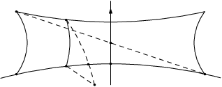
By the triangle inequality,
Define and now take and to be at the same distance from , on opposite sides. Let be the intersection point of with the line through and . Then , and so the cosine formula in the right-angled triangle yields
where . On the other hand, , so it is sufficient to see that for all . This follows from the fact that the function is decreasing on , with limit at infinity. ∎
8.3. Crooked fundamental domains in obtained from strip deformations
Let be the holonomy representations of two convex cocompact hyperbolic structures on a fixed surface. Assume that acts properly discontinuously on . By [Ka], up to switching and we may assume that is “uniformly longer” than in the sense that (1.3) is satisfied. This implies [T1] that the surface is not compact. Note that switching and amounts to conjugating the -action on by the orientation-reversing isometry , which maps left crooked planes to right crooked planes. Assuming that is “uniformly longer” than , we shall prove the existence of a fundamental domain in for that is bounded by finitely many left crooked planes.
By Theorem 1.8, we can realize as a strip deformation of supported on some collection of geodesic arcs on the hyperbolic surface , which cut the surface into topological disks. We proceed as in the infinitesimal case, again using the notation of Section 4. Similarly to Observation 4.4, the strip deformation taking to is described by an assignment of motions to the tiles satisfying the following:
- •
is -equivariant: for all and ,
- •
for any transversely oriented geodesic , bordering tiles on the negative and positive sides respectively, the relative displacement
is hyperbolic with translation axis orthogonal to , oriented in the positive direction; equivalently, by Lemma 4.1.(3’). The translation length of is the width of the strip to be inserted in along the projection of .
To any we associate the crooked plane where
| (8.2) |
Here the square root of a hyperbolic element denotes the hyperbolic element with the same oriented axis but half the translation length. One could think of as the motion of the edge under the strip deformation, which we take to be the average of the motions of the adjacent tiles. Since is -equivariant, is -equivariant and
for all and . We claim that the , for , are pairwise disjoint. Indeed, consider two adjacent edges bounding tiles as in Figure 8. Transversely orient from to , and from to so that the positive half-plane of in (i.e. the connected component of lying on the positive side of for the transverse orientation) contains that of . Then
Since and , Proposition 8.2 implies
hence
| (8.3) |
This shows in particular that the crooked planes and are disjoint whenever border the same tile. As in the Minkowski setting, induction and (8.3) allow us to conclude that for any edges , transversely oriented so that the positive half-plane of in contains that of ,
| (8.4) |
A candidate fundamental domain is then defined as the intersection of the crooked half-spaces corresponding to the half-planes defining a fundamental domain in for . The proof concludes by showing that . This is implied by the following analogue of Lemma 7.6, which shows that the crooked planes , for , do not accumulate on any set.
Lemma 8.5.
For any and any sequence going to infinity,
Proof.
Let be distinct edges bounding a common tile , transversely oriented as in Figure 8. By construction, . Applying (8.1) twice, we see that for any and ,
| (8.5) |
where depends only on the width of the strip along . The inequality remains true when is either a point of or a horoball centered at an endpoint of , and is either a point of or a horoball centerered at an endpoint of , with and disjoint.
To prove the lemma, it is enough to treat the case that is a sequence of distinct edges, each separated from the next by just one tile, and that . For , let be any point of or any horoball centered at an endpoint of , disjoint from . The shortest path from to intersects each at a point . Applying (8.5) to each subsegment, we find
where is the smallest of the finitely many values . Up to conjugation we may assume . Let , where . By definition of , there is a singleton or a horoball centered at an endpoint of such that . Then
By the triangle inequality, . The result follows. ∎
Remark 8.6.
In (8.2), we could have taken
for an arbitrary fixed , not necessarily ; the proof would have worked the same way. (Here .)
Appendix A Realizing the zero cocycle
This appendix is a complement to the discussion of Section 5.2, whose notation and setup we continue with (in particular, we refer to Figure 5). It is not needed for the proofs of Theorems 1.5 and 1.8.
In Section 5.2 we gave a realization, through the map of (4.4), of the zero cocycle as a linear combination of the infinitesimal strip deformation maps by choosing specific geodesic representatives, waists, and widths. In this appendix, we keep the same geodesic representatives (whose extensions to intersect in triples as in Figure 5) but vary the waists; we determine all possible realizations of the zero cocycle supported on the arcs and discuss their geometric significance in relation with Conjecture 1.6.
A.1. Generalized infinitesimal strip deformations
Let be a geodesic hyperideal triangulation of , with set of edges . Recall the notation from Section 4.2.
Definition A.1.
A relative motion map is called a generalized infinitesimal strip deformation if for any transversely oriented edge . The support of is the set of arcs such that is nonzero on the lifts to of . We also refer to the cohomology class in induced by as a generalized infinitesimal strip deformation.
Infinitesimal strip deformations in the sense of Definition 1.4 are generalized infinitesimal strip deformations for which lies in one particular spacelike quadrant of the timelike plane . We will call these strip deformations positive (and their opposites negative) to distinguish them among generalized strip deformations. Generalized infinitesimal strip deformations can also be neither positive nor negative: if for instance is timelike, then the relative motion of the two tiles adjacent to is an infinitesimal rotation centered at a point of .
Generalized infinitesimal strip deformations supported on a single arc form a linear -plane in .
A.2. The point associated with a realization of the zero cocycle
We now work in the setting of Section 5.2: the hyperideal triangulations differ by a single diagonal exchange and have a common refinement . We have four spacelike vectors , scaled so that
| (A.1) |
and our chosen geodesic representatives lift to with
for all (with the convention that ). For simplicity, we henceforth assume that are all distinct in the quotient surface . Recall that and . All edges and carry transverse orientations shown in Figure 5.
For any , we define a -equivariant map supported on the -orbits of the “small” tiles by
| (A.2) |
for all , where is the Minkowski cross-product of Section 4.1. As in Section 4.2, any -equivariant map defines a relative motion map given by
for any tiles adjacent to an edge which is transversely oriented from to .
Lemma A.2.
Let be a -equivariant map with outside the -orbits of . The associated map is a generalized infinitesimal strip deformation (Definition A.1) if and only if for some (unique) .
In this case the support of the generalized infinitesimal strip deformation is contained in . Note that Lemma A.2 holds regardless of how the other geodesic representatives for are chosen.
Proof.
Since outside the -orbits of the , we have outside the -orbits of the and for . By Definition A.1, the fact that is a generalized infinitesimal strip deformations is equivalent to
| (A.3) |
for all . We first check that the space of -equivariant maps for which satisfies (A.3) has dimension . By construction, and . If satisfies (A.3), then we may write
for all , where . Since (A.1) is the only relation between , the condition is equivalent to , and so we may eliminate the and write
where . The condition is equivalent to , which amounts to
i.e. by (A.1). The space of quadruples satisfying this condition has dimension , as announced.
A.3. The case of timelike
Lemma A.3.
If is timelike, then the map associated with is a generalized infinitesimal strip deformation whose support is exactly . The six (nonzero) vectors are all spacelike, i.e. correspond to either positive or negative infinitesimal strip deformations. The corresponding waists on are the respective orthogonal projections of in .
Proof.
From (A.4) and (A.5) we know that and are orthogonal to , hence are zero or spacelike if is timelike. To see that they are nonzero, we note that the planes and are timelike, hence the vectors and are spacelike; in particular, these vectors are not collinear to , and we conclude using (A.4) and (A.5).
A.4. The map of Section 5.2
Recall that the map we constructed in Section 5.2 is given by for all . By (5.7), the associated map satisfies the hypotheses of Lemma A.2, hence for some . We now determine . (This will not be needed afterwards.)
Lemma A.4.
The vector is timelike and satisfies , where is the intersection point of the common perpendicular to and in with the common perpendicular to and .
Proof.
In general, is not the point .
A.5. Link with Conjecture 1.6
The following lemma provides evidence for Conjecture 1.6.
Lemma A.5.
Let the map of Section 1.2 be defined with respect to our choice of geodesic representatives of the arcs of , with waists on that are all orthogonal projections of a common point , and with infinitesimal widths all equal to . Then the image of looks salient at the codimension-2 face shared by and , when seen from the origin of .
Proof.
Recall the linear relation (5.3):
By Claim 3.2.(0) the coefficients are unique up to scale, and by Claim 3.2–(1) we may take and to be positive. The fact that the image of looks salient at the codimension-2 face shared by and is then expressed by
| (A.6) |
Let us prove that this inequality holds.
By definition, the coefficients encode a realization of the zero cocycle by (positive and negative) infinitesimal strip deformations with the given geodesic representatives and waists. By Lemma A.3 and uniqueness of , this realization is of the form for some timelike with . (In particular, for .) Moreover, if varies continuously in while remains in the same component of the timelike cone of , then the signs (positive or negative) of the infinitesimal strip deformations defining remain constant, similar to (5.4). Therefore, since the infinitesimal widths are all equal to , the relation (5.3) has the form
where we set , and for spacelike . Note that the points , for , form a parallelogram in : indeed,
by (A.1). By Lemma A.2, it follows that the , for , form a parallelogram in the spacelike plane . As a consequence,
and so (A.6) holds. ∎
References
- [Ab] H. Abels, Properly discontinuous groups of affine transformations: a survey, Geom. Dedicata 87 (2001), p. 309–333.
- [Au] L. Auslander, The structure of compact locally affine manifolds, Topology 3 (1964), p. 131–139.
- [BM] J. Brock, H. Masur, Coarse and synthetic Weil–Petersson geometry: quasi-flats, geodesics, and relative hyperbolicity, Geom. Topol. 12 (2008), p. 2453–2495.
- [BMNS] J. Brock, Y. Minsky, H. Namazi, J. Souto, Bounded combinatorics and uniform models for hyperbolic 3-manifolds, preprint, arXiv:1312.2293.
- [BCDG] J.-P. Burelle, V. Charette, T. Drumm, W. M. Goldman, Crooked half-spaces, Enseign. Math., to appear.
- [CDG1] V. Charette, T. Drumm, W. M. Goldman, Affine deformations of the three-holed sphere, Geom. Topol. 14 (2010), p. 1355–1382.
- [CDG2] V. Charette, T. Drumm, W. M. Goldman, Finite-sided deformation spaces of complete affine -manifolds, J. Topol., to appear.
- [CDG3] V. Charette, T. Drumm, W. M. Goldman, Proper affine deformations of two-generator Fuchsian groups, in preparation.
- [ChaG] V. Charette, W. M. Goldman, Affine Schottky groups and crooked tilings, in Crystallographic groups and their generalizations (Kortrijk, 1999), p. 69–97, Contemp. Math. 262, American Mathematical Society, Providence, RI, 2000.
- [CFL] V. Charette, D. Francoeur, R. Lareau-Dussault, Fundamental polyhedra in the Einstein Universe, preprint, arXiv:1307:6531.
- [ChoG] S. Choi, W. M. Goldman, Topological tameness of Margulis spacetimes, preprint, 2013.
- [DGK1] J. Danciger, F. Guéritaud, F. Kassel, Geometry and topology of complete Lorentz spacetimes of constant curvature, preprint, arXiv:1306.2240.
- [DGK2] J. Danciger, F. Guéritaud, F. Kassel, Fundamental domains for free groups acting on anti-de Sitter -space, preprint.
- [DGK3] J. Danciger, F. Guéritaud, F. Kassel, Geometry, topology, and moduli spaces of Margulis spacetimes, in preparation.
- [DT] B. Deroin, N. Tholozan, Dominating surface group representations by Fuchsian ones, preprint, arXiv:1311.2919.
- [D] T. Drumm, Fundamental polyhedra for Margulis space-times, Topology 21 (1992), p. 677–683.
- [DG1] T. Drumm, W. M. Goldman, Crooked Planes, Electronic Research Announcements of the American Math. Soc. 1 (1) (1995).
- [DG2] T. Drumm, W.M. Goldman, The geometry of crooked planes, Topology 38 (1999), p. 323–352.
- [F] C. Frances, The conformal boundary of Margulis space-times, C. R. Math. Acad. Sci. Paris 336 (2003), p. 751–756.
- [FG] D. Fried, W. M. Goldman, Three-dimensional affine crystallographic groups, Adv. Math. 47 (1983), p. 1–49.
- [Go] W. M. Goldman, Crooked surfaces and anti-de Sitter geometry, preprint, arXiv:1302.4911.
- [GLM1] W. M. Goldman, F. Labourie, G. A. Margulis, Proper affine actions and geodesic flows of hyperbolic surfaces, Ann. of Math. 170 (2009), p. 1051–1083.
- [GLM2] W. M. Goldman, F. Labourie, G. A. Margulis, in preparation.
- [GLMM] W. M. Goldman, F. Labourie, G. A. Margulis, Y. Minsky, Complete flat Lorentz -manifolds and laminations on hyperbolic surfaces, in preparation.
- [GM] W. M. Goldman, G. A. Margulis, Flat Lorentz -manifolds and cocompact Fuchsian groups, in Crystallographic groups and their generalizations (Kortrijk, 1999), p. 135–145, Contemp. Math. 262, American Mathematical Society, Providence, RI, 2000.
- [Gu] F. Guéritaud, Lengthening deformations of singular hyperbolic tori, preprint, to appear in Boileau Festschrift (J.-P. Otal, ed.), available at http://math.univ-lille1.fr/~gueritau/math.html.
- [GK] F. Guéritaud, F. Kassel, Maximally stretched laminations on geometrically finite hyperbolic manifolds, preprint, arXiv:1307.0256.
- [GKW] F. Guéritaud, F. Kassel, M. Wolff, Compact anti-de Sitter -manifolds and folded hyperbolic structures on surfaces, preprint, arXiv:1311.2804.
- [GL] R. Guo, F. Luo, Cell decompositions of Teichmüller spaces of surfaces with boundary, Pacific J. Math. 253 (2011), p. 423–438.
- [H] G. P. Hazel, Triangulating Teichmüller space using the Ricci flow, PhD thesis, University of California, San Diego, 2004, see http://math.ucsd.edu/thesis/thesis/ghazel/ghazel.pdf.
- [Ka] F. Kassel, Quotients compacts d’espaces homogènes réels ou -adiques, PhD thesis, Université Paris-Sud 11, November 2009, available at http://math.univ-lille1.fr/kassel/.
- [Ke] S. P. Kerckhoff, The Nielsen realization problem, Ann. of Math. 117 (1983), p. 235–265.
- [KR] R. S. Kulkarni, F. Raymond, 3-dimensional Lorentz space-forms and Seifert fiber spaces, J. Differential Geom. 21 (1985), p. 231–268.
- [Ma1] G. A. Margulis, Free completely discontinuous groups of affine transformations (in Russian), Dokl. Akad. Nauk SSSR 272 (1983), p. 785–788.
- [Ma2] G. A. Margulis, Complete affine locally flat manifolds with a free fundamental group, J. Soviet Math. 1934 (1987), p. 129–139, translated from Zap. Naucha. Sem. Leningrad. Otdel. Mat. Inst. Steklov (LOMI) 134 (1984), p. 190–205.
- [MM] H. Masur, Y. Minsky, Geometry of the complex of curves. I. Hyperbolicity, Invent. Math. 138 (1999), p. 103–149.
- [Me] G. Mess, Lorentz spacetimes of constant curvature (1990), Geom. Dedicata 126 (2007), p. 3–45.
- [Mi] J. Milnor, On fundamental groups of complete affinely flat manifolds, Adv. Math. 25 (1977), p. 178–187.
- [P1] R. C. Penner, The decorated Teichmüller space of punctured surfaces, Comm. Math. Phys. 113 (1987), p. 299–339.
- [P2] R. C. Penner, Decorated Teichmüller theory, QGM Master Class Series, European Mathematical Society, Zürich, 2012.
- [PT] A. Papadopoulos, G. Théret, Shortening all the simple closed geodesics on surfaces with boundary, Proc. Amer. Math. Soc. 138 (2010), p. 1775–1784.
- [R] K. Rafi, A combinatorial model for the Teichmüller metric, Geom. Funct. Anal. 17 (2007), p. 936–959.
- [T1] W. P. Thurston, Minimal stretch maps between hyperbolic surfaces, preprint (1986), arXiv:9801039.
- [T2] W. P. Thurston, Earthquakes in two-dimensional hyperbolic geometry, in Low-dimensional topology and Kleinian groups (Coventry/Durham, 1984), p. 91–112, London Math. Soc. Lecture Note Ser. 112, Cambridge University Press, Cambridge, 1986.
- [T] N. Tholozan, Dominating surface group representations and deforming closed anti-de Sitter -manifolds, preprint, arXiv:1403.7479.