Channel Estimation and Optimal Training Design for Correlated MIMO Two-Way Relay Systems in Colored EnvironmentThanks: R. Wang is with the Department of Information and Communications at Tongji University, Shanghai, 201804, P. R. China. Email: liouxingrui@gmail.com. M. Tao is with the Department of Electronic Engineering at Shanghai Jiao Tong University, Shanghai, China. Emails: mxtao@sjtu.edu.cn. H. Mehrpouyan is with the Department of Computer and Electrical Engineering and Computer Science at California State University, Bakersfield, CA, USA. Email: hani.mehr@ieee.org. Y. Hua is with the Department of Electrical Engineering at the University of California, Riverside, CA, USA. Email: yhua@ee.ucr.edu.

Relay assisted cooperative communications has been regarded as one of the most promising techniques in combating long distance channel fading in complex wireless communication systems. One popular example is one-way relaying, which has been well studied in the past decade [1, 2, 3]. Although one-way relaying shows great potential in reducing power consumption, enhancing reliability, and extending coverage, it suffers from low spectral efficiency due to the half-duplex nature of the network. To overcome this disadvantage, by using the idea of network coding, two-way relaying (TWR) has been proposed and has received great attention recently [4]. In fact, TWR can maintain the advantages of traditional relaying while doubling spectrum efficiency.

The improvement in spectrum efficiency in TWR is achieved by applying self-interference cancelation at each source node and extracting the desired information from the received network-coded messages. In this case, the accuracy of the self-interference cancelation process significantly affects the performance of TWR systems. Moreover, when using the popular amplify-and-forward (AF) relaying strategy, the accuracy of self-interference cancelation process is highly dependent on the precision of the channel estimation process. Thus, obtaining highly accurate channel state information (CSI) becomes more important in TWR systems compared to traditional one-way relaying systems. In fact, devising new channel estimation schemes for TWR systems has received great attention recently. For example, in [5], the authors propose to estimate the cascaded channel of TWR systems under the AF relaying strategy. By using multiple phase shift keying (M-PSK) training symbols, blind and partially-blind channel estimators are investigated in [6, 7]. Different from [5, 6, 7], where flat fading channel are assumed, the authors in [8] investigate time varying channel estimation via a new complex-exponential basis expansion model. Moreover, in [9, 10], the channel estimation process for TWR is extended to the scenario of orthogonal frequency division multiplexing (OFDM) systems.

It is worth noting that the works summarized above are concerned with single-antenna TWR systems. As expected, the multi-antenna or multi-input multi-output (MIMO) technique can be introduced to TWR systems to further improve transmission reliability and bandwidth efficiency. One efficient way to realize such performance improvement is to exploit the estimated CSI for the application of source and relay precoding [11, 12, 13, 14]. Therefore, in MIMO TWR systems, in addition to affecting the performance of self-interference cancelation, inaccurate channel estimation also imposes a negative effect on the precoder design.

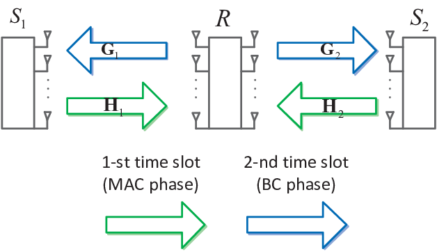
Fig. 1 depicts a MIMO TWR setup. Let us denote the process of data transmission from the source nodes to the relay and relay to the source nodes as the broadcasting (BC) and multiple access (MAC) phases, respectively. In [15], a MIMO channel estimator is proposed that uses the self-interference as a training sequence to estimate the channel matrices corresponding to the BC phase. In [16], the performances of different channel estimators, including individual and cascaded channel estimators, are compared based on the least squares (LS) criterion. In [17], an LS estimator is used to obtain the cascaded channel matrices corresponding to the BC and MAC phases using a single carrier cyclic prefix. Note that in the contributions of [15, 16, 17], the channel statistics, whether cascaded channels or the individual channels, are assumed to be unknown deterministic matrices. Based on the estimation theory, if channel statistics are known, the channel estimation can be conducted under the Bayesian framework and the estimation accuracy can be further enhanced. Hence, by taking these statistics into account, we seek to improve upon the channel estimators in [15, 16, 17].

Very recently, the authors in [18, 19] independently investigate the minimum mean-square-error (MMSE) channel estimation for TWR systems based on a correlated Gaussian MIMO channel model. In particular, in [18], the cascaded channel matrices for AF TWR systems are estimated and the training sequences at the two source nodes are optimized to minimize the total channel estimation MSE. Different from [18], the authors in [19] aim to estimate the individual channel matrices for each link. To reach this goal, two different estimation schemes, i.e., the superimposed channel training and the two-stage channel estimation schemes, are proposed. In addition, the training sequences at the two source nodes, as well as, at the relay node are jointly optimized to improve channel estimation accuracy.

In this paper, similar to [15, 16, 17, 18, 19], while assuming that the channel statistics are known, we analyze and devise channel estimators for correlated MIMO TWR systems. Specifically, we consider the Kronecker-structured channel model, such that the individual channel matrices can be estimated based on the Bayesian framework. However, unlike [18, 19], we take into account the interference from the nearby users. Thus, in this model, the disturbance at the source nodes and the relay node consists of both noise and interference. Note that the considered colored estimation environment may be more practical for applications in today’s more densely deployed wireless networks. Although channel estimation in point-to-point MIMO systems in colored environments has been studied in [20, 21], to the best of our knowledge, this topic has not been addressed in the TWR scenario.

To enhance TWR performance, we seek to estimate the individual channel matrices corresponding to source-to-relay and relay-to-source links, see Fig. 1. To this end, a new two-phase estimation scheme is proposed, where the bidirectional transmission of a TWR system is decomposed into the MAC and BC phases. For the MAC and BC phases, the channel estimation is performed at the relay node and two source/user nodes, respectively. The proposed estimation scheme is different from the ones in [18, 19], where the channel estimation is assumed to only be conducted at the user ends. As such, our proposed estimation scheme can more efficiently support precoding at the relay since it requires significantly less feedback overhead [13, 22, 23]. Based on the proposed estimation scheme, we derive the optimal linear MMSE (LMMSE) estimator for each phase. Next, the corresponding training design problems are formulated with the aim of minimizing the total MSE of channel estimation process for each phase. The training design problem considered here is different from that of [18, 19], since we take into account the effect of colored disturbances caused by interference at the relay node and user ends. Moreover, the training design scenarios for point-to-point systems in [20, 21] are different from the scenario under consideration in this paper, since our proposed training sequence design is optimized to simultaneously enhance channel estimation accuracy over both links in the BC and MAC phases. Although, for the general scenario, it is difficult to derive the optimal training sequence structures as in [18, 19, 20, 21], we propose two iterative design algorithms to solve the training design problems. These algorithms are verified to converge quickly to the near optimal solution and to not be sensitive to the initialization process. For some special cases, where the covariance matrices of the channels or disturbances have specific forms, two specific approaches are applied to obtain the optimal training sequences: 1) the original problem is converted into a standard convex optimization problem; 2) the optimal structures of the training sequences are first derived and then used to reduce the original non-convex problem into a simple power allocation problem. Finally, to reduce training overhead, the minimum required training length for channel estimation in both the MAC and BC phases are derived and extensive simulations are carried out to support the findings of the paper.

The rest of the paper is organized as follows. In Section II, we present the system model. The optimal LMMSE estimators for both MAC and BC phases are derived in Section III. The training designs for the MAC and the BC phases are analyzed in Section IV and V, respectively. Simulation results are provided in Section VI. Finally, we conclude the paper in Section VII.

Notations: $\cal E(\cdot)$ denotes the expectation operator. $\otimes$ denotes the Kronecker operator. ${\rm vec}(\cdot)$ signifies the matrix vectorization operator. Superscripts ${\bf A}^{T}$, ${\bf A}^{*}$, and ${\bf A}^{H}$ denote the transpose, conjugate, and conjugate transpose of matrix $\bf A$, respectively. ${\rm Tr}({\bf A})$, ${\bf A}^{-1}$, $\det({\bf A})$, and ${\rm Rank}(\bf A)$ stand for the trace, inverse, determinant, and rank of ${\bf A}$, respectively. ${\bm{\lambda}}({\bf A})$ denotes a vector containing eigenvalues of ${\bf A}$. ${\rm Blkdiag}({\bf A}_{1},{\bf A}_{2},\cdots,{\bf A}_{N})$ denotes a block diagonal matrix constructed by matrices ${\bf A}_{i}$, for $\forall i$. ${\rm Diag}(\bf a)$ denotes a diagonal matrix with ${\bf a}$ being its diagonal entries. ${\bf A}(n:m,:)$ and ${\bf A}(:,n:m)$ denote the sub-matrices constructed by $n$ to $m$ rows and $n$ to $m$ columns of ${\bf A}$, respectively. $||{\bf A}||^{2}_{F}$ denotes the Frobenius norm of ${\bf A}$. ${\bf 0}$ and ${\bf I}$ denote the zero and identity matrices, respectively. ${\Re}(z)$ denotes the real part of complex variable $z$. The distribution of a circular symmetric complex Gaussian vector with mean vector $\bf x$ and covariance matrix ${\bf\Sigma}$ is denoted by ${\cal CN}({\bf x},{\bf\Sigma})$. ${\mathbb{C}}^{x\times y}$ denotes the space of complex $x\times y$ matrices. $\mathbb{S}^{N}$ and $\mathbb{S}^{N}_{+}$ denote the set of symmetric $N\times N$ matrices and the set of positive semidefinite $N\times N$ matrices, respectively. ${\bf x}\preccurlyeq{\bf y}$ denotes that the vector $\bf y$ majorizes the vector $\bf x$.

Consider a TWR system, where source nodes $S_{1}$ and $S_{2}$ intend to exchange messages with one another through a relay node $R$. $S_{1}$, $R$, and $S_{2}$ are assumed to be equipped with $N_{1}$, $M$, and $N_{2}$ antennas, respectively. The channel matrices from $S_{1}$ and $S_{2}$ to $R$ are denoted by ${\bf H}_{1}$ and ${\bf H}_{2}$, respectively, and the channel matrices from $R$ to $S_{1}$ and $S_{2}$ are denoted by ${\bf G}_{1}$ and ${\bf G}_{2}$, respectively.

Signal transmission within the TWR system is assumed to be achieved in two time slots. In the first phase, referred to as the MAC phase, the source node $S_{i}$, for $i=1,2$, transmits its signal to the relay node $R$, while in the second phase, referred to as the BC phase, the relay node $R$ forwards the its combined received signal to the two source nodes $S_{1}$ and $S_{2}$. The proposed channel estimator aims to obtain the individual channels of the two hops, i.e., $\{{\bf H}_{1},{\bf H}_{2},{\bf G}_{1},{\bf G}_{2}\}$. Note that different from the cases studied in [5, 18], where the cascaded channels are estimated, here, the individual channel matrices are estimated. This approach enhances precoding design and/or power allocation at the relay node, which can further improve the overall system performance [11, 12, 13, 14, 22, 23].

Following the transmission model in Fig. 1, we assume that ${\bf H}_{1}$ and ${\bf H}_{2}$ are estimated in the MAC phase via the training signals sent from the two source nodes, and ${\bf G}_{1}$ and ${\bf G}_{2}$ are estimated in the BC phase via the training signal transmitted from the relay.

The received training signals at the relay node in the MAC phase can be expressed as

$${\bf y}_{R}(t)={\bf H}_{1}{\bf s}_{1}(t)+{\bf H}_{2}{\bf s}_{2}(t)+{\bf n}_{R}(t),$$

(1)

where ${\bf s}_{i}(t)\in\mathbb{C}^{N_{i}\times 1}$ denotes the training signal at the source $S_{i}$ and ${\bf n}_{R}(t)\in\mathbb{C}^{M\times 1}$ represents the correlated Gaussian disturbance at the relay node. ${\bf n}_{R}(t)$ models the total background noise as well as the interference from adjacent communication links. ${\bf n}_{R}(t)$ is modeled as a stochastic process with respect to the time variable $t$ [20, 21, 24]. Here, the channel matrix ${\bf H}_{i}\in\mathbb{C}^{M\times N_{i}}$ is modeled by the Rayleigh fading with mean zero and covariance ${\bf Z}_{H_{i}}\in\mathbb{S}^{MN_{i}\times MN_{i}}_{+}$, i.e., ${\rm vec}({\bf H}_{i})\sim\mathcal{CN}({\bf 0},{\bf Z}_{H_{i}})$. To estimate the channel matrices at the relay, the source nodes typically need to send a sequence of known training signals. Assuming training sequences have a length of $L_{S}$, the received signal in (1) can be written in matrix from as

$${\bf Y}_{R}={\bf H}_{1}{\bf S}_{1}+{\bf H}_{2}{\bf S}_{2}+{\bf N}_{R},$$

(2)

where ${\bf Y}_{R}\triangleq[{\bf y}_{R}(1),{\bf y}_{R}(2),\cdots,{\bf y}_{R}(L_{S})]\in\mathbb{C}^{M\times L_{S}}$, ${\bf S}_{i}\triangleq[{\bf s}_{1}(1),{\bf s}_{1}(2),\cdots,{\bf s}_{1}(L_{S})]\in\mathbb{C}^{N_{i}\times L_{S}}$ and ${\bf N}_{R}\triangleq[{\bf n}_{R}(1),{\bf n}_{R}(2),\cdots,{\bf n}_{R}(L_{S})]\in\mathbb{C}^{M\times L}$. Here, the disturbance ${\bf N}_{R}$ is modeled as ${\rm vec}({\bf N}_{R})\sim\mathcal{CN}({\bf 0},{\bf K}_{R})$ with ${\bf K}_{R}\in\mathbb{S}^{ML_{S}\times ML_{S}}_{+}$. Suppose that the source node $S_{i}$ has a maximum power of $\tau_{i}$ during the channel estimation phase, the training sequence ${\bf S}_{i}$ should fulfill the following power constraint

$${\rm Tr}({\bf S}_{i}{\bf S}^{H}_{i})\leq\tau_{i}.$$

(3)

In the BC phase, the received training signals at the source nodes are given by

$${\bf y}_{i}(t)={\bf G}_{i}{\bf s}_{R}(t)+{\bf n}_{i}(t),~i=1,2$$

(4)

where ${\bf s}_{R}(t)\in\mathbb{C}^{M\times 1}$ denotes the training signal at the relay node and ${\bf n}_{i}(t)\in\mathbb{C}^{N_{i}\times 1}$ represents the correlated Gaussian disturbance at the node $S_{i}$. The channel matrix ${\bf G}_{i}\in\mathbb{C}^{M\times N_{i}}$ is modeled by a Rayleigh fading parameter with mean zero and covariance ${\bf Z}_{G_{i}}\in\mathbb{S}^{MN_{i}\times MN_{i}}_{+}$, i.e., ${\rm vec}({\bf G}_{i})\sim\mathcal{CN}({\bf 0},{\bf Z}_{G_{i}})$. As in (1), here, the disturbance term ${\bf n}_{i}(t)$ also includes the total background noise and interference from nearby communication nodes. By rewriting (4) into matrix form, we have

$$\begin{split}{\bf Y}_{i}={\bf G}_{i}{\bf S}_{R}+{\bf N}_{i},~i=1,2,\end{split}$$

(5)

where ${\bf Y}_{i}\triangleq[{\bf y}_{i}(1),{\bf y}_{i}(2),\cdots,{\bf y}_{i}(L_{R})]\in\mathbb{C}^{N_{i}\times L_{R}}$, ${\bf S}_{R}\triangleq[{\bf s}_{R}(1),{\bf s}_{R}(2),\cdots,{\bf s}_{R}(L_{R})]\in\mathbb{C}^{N_{i}\times L_{R}}$ and ${\bf N}_{i}\triangleq[{\bf n}_{i}(1),{\bf n}_{i}(2),\cdots,{\bf n}_{i}(L_{R})\in\mathbb{C}^{M\times L_{R}}$. The disturbance ${\bf N}_{i}$ is modeled as ${\rm vec}({\bf N}_{i})\sim\mathcal{CN}({\bf 0},{\bf K}_{i})$ with ${\bf K}_{i}\in\mathbb{S}^{N_{i}L_{R}\times N_{i}L_{R}}$. Here, we assume that the training sequence length at the relay is $L_{R}$. The following condition must be met to satisfy the power constraint at the relay node

$$\begin{split}{\rm Tr}({\bf S}_{R}{\bf S}^{H}_{R})\leq\tau_{R}.\end{split}$$

(6)

In (6), $\tau_{R}$ denotes the maximum power at the relay node during the training phase.

In this work, we assume that the channel covariance matrices ${\bf Z}_{H_{i}}$ and ${\bf Z}_{G_{i}}$ and the covariance of disturbance ${\bf K}_{R}$ and ${\bf K}_{i}$, for $i=1,2$, are structured and their statistics are known. Let us first focus on the properties of the channel statistics.

The correlation amongst the channel parameters can be caused by insufficient antenna spacing as verified by measurements in [25, 26]. Accordingly, the channel matrices are assumed to follow the Kronecker-structured model, i.e., the covariance matrices are separated between the transmitter and receiver sides and given by ${\bf Z}_{H_{i}}={\bf Z}_{t,{H_{i}}}\otimes{\bf Z}_{r,H}$, ${\bf Z}_{G_{i}}={\bf Z}_{t,G}\otimes{\bf Z}_{r,{G_{i}}}$ for $j={1,2}$. Here, indexes ‘$t$’ and ‘$r$’ denote ‘transmitter’ and ‘receiver’, respectively. In addition, since the channels ${\bf H}_{1}$ and ${\bf H}_{2}$ terminate at the relay node and the channels ${\bf G}_{1}$ and ${\bf G}_{2}$ begin at the relay node, we have that ${\bf Z}_{r,H_{1}}={\bf Z}_{r,H_{2}}={\bf Z}_{r,H}$ and ${\bf Z}_{t,G_{1}}={\bf Z}_{t,G_{2}}={\bf Z}_{t,G}$. Using the Kronecker model and the above definitions, the channel matrices can be expressed as [18, 19, 20, 21, 24]

$$\begin{split}{\bf H}_{i}={\bf C}_{r,H}{\bf W}_{H_{i}}{\bf C}^{T}_{t,H_{i}},~{\bf G}_{i}={\bf C}_{r,G_{i}}{\bf W}_{G_{i}}{\bf C}^{T}_{t,G},~i=1,2\end{split}$$

(7)

where ${\bf Z}_{t,H_{i}}={\bf C}_{t,H_{i}}{\bf C}^{H}_{t,H_{i}}$, ${\bf Z}_{r,H}={\bf C}_{r,H}{\bf C}^{H}_{r,H}$, ${\bf Z}_{t,G}={\bf C}_{t,G}{\bf C}^{H}_{t,G}$, and ${\bf Z}_{r,G_{i}}={\bf C}_{r,G_{i}}{\bf C}^{H}_{r,G_{i}}$. ${\bf W}_{H_{i}}$ and ${\bf W}_{G_{i}}$ are unknown matrices, where their entries are modeled by $\mathcal{CN}(0,1)$.

The structured disturbance covariance ${\bf K}_{i}$, for $i\in\{R,1,2\}$, are assumed to be modeled by [20, 21, 24]

$$\begin{split}{\bf K}_{i}={\bf K}_{q,i}\otimes{\bf K}_{r,i},~i=R,1,2,\end{split}$$

(8)

where ${\bf K}_{q,1}/{\bf K}_{q,2}\in\mathbb{C}^{L_{S}\times L_{S}}$, ${\bf K}_{q,R}\in\mathbb{C}^{L_{R}\times L_{R}}$ denote the temporal covariance matrix and ${\bf K}_{r,1}\in\mathbb{C}^{N_{1}\times N_{1}}$, ${\bf K}_{r,2}\in\mathbb{C}^{N_{2}\times N_{2}}$, and ${\bf K}_{r,R}\in\mathbb{C}^{M\times M}$ denote the received spatial covariance matrix. Moreover, it is assumed that ${\bf K}_{r,1}$, ${\bf K}_{r,2}$, and ${\bf K}_{r,R}$ share the same eigenvectors with ${\bf Z}_{r,{G_{1}}}$, ${\bf Z}_{r,{G_{2}}}$ and ${\bf Z}_{r,H}$, respectively. This assumption is valid when the disturbances are either spatially uncorrelated or share the same spatial structure as the channel [24, 21]. In addition, as summarized in [21], this assumption models the following scenarios: 1) Additive noise-limited scenario, ${\bf K}_{r,i}=\mu_{i}{\bf I}$ with $\mu_{i}$ being some variance, for $i=R,1,2$; 2) Interference-limited scenario, ${\bf K}_{r,i}={\bf Z}_{r,{G_{i}}}$, for $i=1,2$, and ${\bf K}_{r,R}={\bf Z}_{r,H}$; 3) Additive noise and temporally uncorrelated interference scenario, ${\bf K}_{r,i}=\mu_{i}{\bf I}+\nu_{i}{\bf Z}_{r,{G_{i}}}$, for $i=1,2$, and ${\bf K}_{r,R}=\mu_{R}{\bf I}+\nu_{R}{\bf Z}_{r,H}$ with $\nu_{i}$, for $i=R,1,2$, being the number of interfering users; and 4) Additive noise and spatially uncorrelated interference scenario, ${\bf K}_{r,i}={\bf I}$.

The singular value decomposition (SVD) of ${\bf Z}_{t,{H_{i}}}$, ${\bf Z}_{r,H}$, ${\bf Z}_{t,G}$, and ${\bf Z}_{r,{G_{i}}}$ are given by

$$\begin{split}{\bf Z}_{a,b}={\bf U}_{a,b}{\bm{\Sigma}}_{a,b}{\bf U}^{H}_{a,b},~a\in\{r,t\},b\in\{H,H_{1},H_{2},G,G_{1},G_{2}\},\end{split}$$

(9)

where ${\bf U}_{a,b}$ denotes the unitary eigenvector matrix and ${\bm{\Sigma}}_{a,b}$ is a diagonal matrix with $[{\bm{\Sigma}}_{a,b}]_{n,n}={\sigma}_{a,b,n}$ being the $n$-th eigenvalue of ${\bf Z}_{a,b}$. Accordingly, the SVD decomposition of ${\bf C}_{a,b}$ is denoted by ${\bf C}_{a,b}={\bf U}_{a,b}{\bm{\Sigma}}^{1/2}_{a,b}\tilde{{\bf U}}^{H}_{a,b}$ with $\tilde{{\bf U}}_{a,b}$ represting a unitrary matrix. The SVD decomposition of ${\bf K}_{q,i}$ and ${\bf K}_{r,i}$ is denoted by

$${\bf K}_{a,b}={\bf V}_{a,b}{\bm{\Delta}}_{a,b}{\bf V}^{H}_{a,b},~a\in\{r,t\},b\in\{1,2,R\},$$

(10)

where ${\bf V}_{a,b}$ denotes the unitary eigenvector matrix, ${\bm{\Delta}}_{a,b}$ is a diagonal matrix with $[{\bm{\Delta}}_{a,b}]_{n,n}={\delta}_{a,b,n}$ being the $n$-th eigenvalue of ${\bf K}_{a,b}$. As mentioned before, it is assumed that ${\bf V}_{r,1}={\bf U}_{r,G_{1}}$, ${\bf V}_{r,2}={\bf U}_{r,G_{2}}$ and ${\bf V}_{r,R}={\bf U}_{r,H}$.

Following the proposed estimation scheme in Section II, we next obtain the channel estimates based on (2) and (5). For the estimation during the MAC phase, we rewrite (2) as

$\displaystyle{\bf Y}_{R}={\bf C}_{r,H}{\bf W}_{H_{1}}{\bf C}^{T}_{t,H_{1}}{\bf S}_{1}+{\bf C}_{r,H}{\bf W}_{H_{2}}{\bf C}^{T}_{t,H_{2}}{\bf S}_{2}+{\bf N}_{R}={\bf C}_{r,H}{\bf W}_{H}{\bf C}^{T}_{t,H}{\bf S}+{\bf N}_{R},$

(11)

where ${\bf W}_{H}\triangleq[{\bf W}_{H_{1}},{\bf W}_{H_{2}}]$, ${\bf C}^{T}_{t,H}\triangleq{\rm Blkdiag}({\bf C}^{T}_{t,H_{1}},{\bf C}^{T}_{t,H_{2}})$, and ${\bf S}\triangleq[{\bf S}^{T}_{1},{\bf S}^{T}_{2}]^{T}$. Vectorizing ${\bf Y}_{R}$ in (11) and applying the identity

$\displaystyle\begin{split}{\rm vec}({\bf A}{\bf B}{\bf C})=({\bf C}^{T}\otimes{\bf A}){\rm vec}({\bf B}),\end{split}$

(12)

we can rewrite (11) into

$$\begin{split}{\bf y}_{R}=\left({\bf S}^{T}{\bf C}_{t,H}\otimes{\bf C}_{r,H}\right){\bf w}_{H}+{\bf n}_{R},\end{split}$$

(13)

where ${\bf y}_{R}\triangleq{\rm vec}({\bf Y}_{R})$, ${\bf w}_{H}\triangleq{\rm vec}({\bf W}_{H})$ and ${\bf n}_{R}\triangleq{\rm vec}({\bf N}_{R})$. The estimation of ${\bf w}_{H}$ based on the LMMSE criterion can be obtained as $\hat{{\bf w}}_{H}={\bf T}_{R}{\bf y}_{R}$. The estimation matrix ${\bf T}_{R}$ has the following form [27]

$$\vskip-12.0pt\begin{split}{\bf T}_{R}=\mathfrak{R}_{w_{h}y_{R}}\mathfrak{R}^{-1}_{y_{R}y_{R}}.\end{split}$$

(14)

where

$$\begin{split}\mathfrak{R}_{w_{h}y_{R}}\triangleq&{\cal E}({\bf w}_{H}{\bf y}^{H}_{R})={\bf C}^{H}_{t,H}{\bf S}^{*}\otimes{\bf C}^{H}_{r,H}\\ \mathfrak{R}_{y_{R}y_{R}}\triangleq&{\cal E}({\bf y}_{R}{\bf y}^{H}_{R})=\left({\bf S}^{T}{\bf C}_{t,H}\otimes{\bf C}_{r,H}\right)\left({\bf S}^{T}{\bf C}_{t,H}\otimes{\bf C}_{r,H}\right)^{H}+{\bf K}_{R}={\bf S}^{T}{\bf C}_{t,H}{\bf C}^{H}_{t,H}{\bf S}^{*}\otimes{\bf C}_{r,H}{\bf C}^{H}_{r,H}+{\bf K}_{R}.\end{split}$$

Let us define ${\bf h}\triangleq{\rm vec}({\bf H})=\left({\bf C}_{t,H}\otimes{\bf C}_{r,H}\right){\bf w}$ with ${\bf H}\triangleq[{\bf H}_{1},{\bf H}_{2}]$, the resulting estimation error, or mean-square-error (MSE), $e_{R}$ can be derived as

$$\begin{split}e_{R}=&{\cal E}\left(||{\bf h}-\hat{{\bf h}}||^{2}_{2}\right)\\ =&{\rm Tr}\left[{\bf C}_{0,H}({\bf w}_{H}-\hat{{\bf w}}_{H})({\bf w}_{H}-\hat{{\bf w}}_{H})^{H}\right]\\ =&{\rm Tr}\left[{\bf C}_{0,H}({\bf w}_{H}-{\bf T}_{R}{\bf y}_{R})({\bf w}_{H}-{\bf T}_{R}{\bf y}_{R})^{H}\right],\end{split}$$

where ${\bf C}_{0,H}\triangleq{\bf C}^{H}_{t,H}{\bf C}_{t,H}\otimes{\bf C}^{H}_{r,H}{\bf C}_{r,H}$. Substituting ${\bf T}_{R}$ into (III) and using the matrix identity $({\bf I}+{\bf A}{\bf B})^{-1}={\bf I}-{\bf A}({\bf I}+{\bf B}{\bf A})^{-1}{\bf B}$, we obtain the following more compact form for $e_{R}$

$$e_{R}={\rm Tr}\left[{\bf C}_{0,H}\left({\bf I}+\left({\bf S}^{T}{\bf C}_{t,H}\otimes{\bf C}_{r,H}\right)^{H}{\bf K}^{-1}_{R}\left({\bf S}^{T}{\bf C}_{t,H}\otimes{\bf C}_{r,H}\right)\right)^{-1}\right].$$

(15)

Note that since the channel estimation model in (13) is linear and Gaussian, the proposed LMMSE estimator is equivalent to the optimal MMSE estimator.

During the BC phase, the channel estimation should be based on the received signal in (5). By vectorizing ${\bf Y}_{i}$ in (5), we have

$$\begin{split}{\bf y}_{i}=\left({\bf S}^{T}_{R}{\bf C}_{t,G}\otimes{\bf C}_{r,G_{i}}\right){\bf w}_{G_{i}}+{\bf n}_{i},~i=1,2\end{split}$$

(16)

where ${\bf y}_{i}\triangleq{\rm vec}({\bf Y}_{i})$, ${\bf w}_{G_{i}}\triangleq{\rm vec}({\bf W}_{G_{i}})$, and ${\bf n}_{i}\triangleq{\rm vec}({\bf N}_{i})$. Similar to steps above, the estimation MSE of ${\bf g}_{i}$ can be obtained as

$$\begin{split}e_{i}&={\cal E}\left(||{\bf g}_{i}-\hat{{\bf g}}_{i}||^{2}_{2}\right)={\rm Tr}\left[{\bf C}_{0,G_{i}}({\bf w}_{G_{i}}-\hat{{\bf w}}_{G_{i}})({\bf w}_{G_{i}}-\hat{{\bf w}}_{G_{i}})^{H}\right]\\ &={\rm Tr}\left[{\bf C}_{0,G_{i}}({\bf w}_{H}-{\bf T}_{i}{\bf y}_{i})({\bf w}_{H}-{\bf T}_{i}{\bf y}_{i})^{H}\right],~i=1,2\end{split}$$

(17)

where ${\bf C}_{0,G_{i}}\triangleq{\bf C}^{H}_{t,G}{\bf C}_{t,G}\otimes{\bf C}^{H}_{r,G_{i}}{\bf C}_{r,G_{i}}$ and

$$\begin{split}{\bf T}_{i}=\mathfrak{R}_{w_{G_{i}}y_{i}}\mathfrak{R}^{-1}_{y_{i}y_{i}}.\end{split}$$

(18)

In (18),

$$\begin{split}\mathfrak{R}_{w_{G_{i}}y_{i}}=&{\cal E}({\bf w}_{G_{i}}{\bf y}^{H}_{i})={\bf C}^{H}_{t,G}{\bf S}^{*}_{R}\otimes{\bf C}^{H}_{r,G_{i}}\\ \mathfrak{R}_{y_{i}y_{i}}=&{\cal E}({\bf y}_{i}{\bf y}^{H}_{i})=\left({\bf S}^{T}_{i}{\bf C}_{t,G}\otimes{\bf C}_{r,G_{i}}\right)\left({\bf S}^{T}_{R}{\bf C}_{t,G}\otimes{\bf C}_{r,G_{i}}\right)^{H}+{\bf K}_{i}={\bf S}^{T}_{R}{\bf C}_{t,G}{\bf C}^{H}_{t,G}{\bf S}^{*}_{R}\otimes{\bf C}_{r,G_{i}}{\bf C}^{H}_{r,G_{i}}+{\bf K}_{i}.\end{split}$$

By substituting ${\bf T}_{i}$ into (17), we obtain

$$\begin{split}e_{i}&={\rm Tr}\left[{\bf C}_{0,G_{i}}\left({\bf I}+\left({\bf S}^{T}_{R}{\bf C}_{t,G}\otimes{\bf C}_{r,G_{i}}\right)^{H}{\bf K}^{-1}_{i}\left({\bf S}^{T}_{R}{\bf C}_{t,G}\otimes{\bf C}_{r,G_{i}}\right)\right)^{-1}\right].\end{split}$$

(19)

In this section, the design of the training sequences for the MAC phase are analyzed. Namely, we shall optimize the training sequences ${\bf S}_{1}$ and ${\bf S}_{2}$ subject to two source power constraints to minimize the total estimation MSE, i.e., $e_{R}$ in (III). The corresponding training sequence optimization problem can be formulated as

$$\begin{split}\min_{{\bf S}_{1},{\bf S}_{2}}~~&{\rm Tr}\left[{\bf C}_{0,H}\left({\bf I}+\left({\bf S}^{T}{\bf C}_{t,H}\otimes{\bf C}_{r,H}\right)^{H}{\bf K}^{-1}_{R}\left({\bf S}^{T}{\bf C}_{t,H}\otimes{\bf C}_{r,H}\right)\right)^{-1}\right]\\ {\rm s.t.}~~&{\rm Tr}({\bf S}_{i}{\bf S}^{H}_{i})\leq\tau_{i},~i=1,2.\end{split}$$

(20)

Before solving (20), we first introduce the following lemma that deals with the minimum length of the training sequence ${\bf S}$, $L_{S}$.

With the minimum length of the training sequences determined, we seek to solve the non-convex optimization problem in (20) with respect to ${\bf S}_{1}$ and ${\bf S}_{2}$. Although the objective function in (20) has a similar form to that of point-to-point systems, there are two power constraints in (20) that make the problem of solving this non-convex optimization problem more difficult than that of point-to-point systems in [20, 21]. In order to proceed, we first note that $e_{R}$ in (15) can be obtained by substituting (14) into (III). Thus, to make the problem tractable, we propose an iterative algorithm, which decouples the primal problem into two sub-problems and solves each of them in an alternating approach. Let us rewrite (15) into the following form

$$\begin{split}\tilde{e}_{R}=&{\rm Tr}\left[{\bf C}_{0,H}({\bf w}_{H}-{\bf T}_{R}{\bf y}_{R})({\bf w}_{H}-{\bf T}_{R}{\bf y}_{R})^{H}\right]\\ =&{\rm Tr}\left[{\bf C}_{0,H}-\left({\bf S}^{T}{\bf C}_{t,H}\otimes{\bf C}_{r,H}\right)^{H}{\bf T}^{H}_{R}{\bf C}^{H}_{0,H}-{\bf C}_{0,H}{\bf T}_{R}\left({\bf S}^{T}{\bf C}_{t,H}\otimes{\bf C}_{r,H}\right)\right.\\ &+\left.{\bf C}_{0,H}{\bf T}_{R}\left({\bf S}^{T}{\bf C}_{t,H}\otimes{\bf C}_{r,H}\right)\times\left({\bf S}^{T}{\bf C}_{t,H}\otimes{\bf C}_{r,H}\right)^{H}{\bf T}^{H}_{R}+{\bf C}_{0,H}{\bf T}_{R}{\bf K}_{R}{\bf T}^{H}_{R}\right].\end{split}$$

(21)

Then, the optimization problem in (20) is equivalent to

$$\begin{split}&\min_{{\bf T}_{R},{\bf S}_{1},{\bf S}_{2}}~~\tilde{e}_{R}\\ &{\rm s.t.}~~{\rm Tr}({\bf S}_{i}{\bf S}^{H}_{i})\leq\tau_{i},~i=1,2.\end{split}$$

(22)

In the first subproblem, we intend to optimize the LMMSE estimator matrix ${\bf T}_{R}$ for a given ${\bf S}_{1}$ and ${\bf S}_{2}$. Since ${\bf T}_{R}$ is not related to the the power constraint, the problem simplifies to an unconstrained optimization problem given by

$$\begin{split}\min_{{\bf T}_{R}}~~\tilde{e}_{R}.\end{split}$$

(23)

Given that (23) is convex with respect to ${\bf T}_{R}$, by setting its gradient to zero, it can be shown that the optimal ${\bf T}_{R}$ is equal to (14).

In the second subproblem, the training sequences ${\bf S}_{1}$ and ${\bf S}_{2}$ need to be optimized for a given ${\bf T}_{R}$ by solving the following optimization problem

$$\begin{split}&\min_{{\bf S}_{1},{\bf S}_{2}}~~\tilde{e}_{R}\\ &{\rm s.t.}~~{\rm Tr}({\bf S}_{i}{\bf S}^{H}_{i})\leq\tau_{i},~i=1,2.\end{split}$$

(24)

Next, it is shown that the optimization problem in (24) can be transformed into a convex quadratically constrained quadratic programable (QCQP) problem [28]. To achieve this goal, we first reformulate the last term in (21) as

$$\begin{split}&{\rm Tr}\left[{\bf C}_{0,H}{\bf T}_{R}\left({\bf S}^{T}{\bf C}_{t,H}\otimes{\bf C}_{r,H}\right)\left({\bf S}^{T}{\bf C}_{t,H}\otimes{\bf C}_{r,H}\right)^{H}{\bf T}^{H}_{R}\right]\\ \overset{(a)}{=}&{\rm Tr}\left[{\bf T}^{H}_{R}{\bf C}_{0,H}{\bf T}_{R}({\bf S}^{T}\otimes{\bf I})({\bf C}_{t,H}{\bf C}^{H}_{t,H}\otimes{\bf C}_{r,H}{\bf C}^{H}_{r,H})({\bf S}^{*}\otimes{\bf I})\right]\\ \overset{(b)}{=}&{\rm vec}({\bf S}\otimes{\bf I})^{H}\left({\bf T}^{H}_{R}{\bf C}_{0,H}{\bf T}_{R}\otimes{\bf C}^{T}_{tr}\right){\rm vec}({\bf S}\otimes{\bf I})\\ \overset{(c)}{=}&{\bf s}^{H}{\bf E}^{H}\left({\bf T}^{H}_{R}{\bf C}_{0,H}{\bf T}_{R}\otimes{\bf C}^{T}_{tr}\right){\bf E}{\bf s},\end{split}$$

(25)

where ${\bf C}_{tr}\triangleq{\bf C}_{t,H}{\bf C}^{H}_{t,H}\otimes{\bf C}_{r,H}{\bf C}^{H}_{r,H}$, ${\bf s}\triangleq{\rm vec}({\bf S})$, ${\bf E}\triangleq{\rm Blkdiag}(\tilde{{\bf E}}_{(1)},\tilde{{\bf E}}_{(2)},\cdots,\tilde{{\bf E}}_{(L_{S})})$, $\tilde{{\bf E}}_{(i)}=\tilde{{\bf E}}$, $\tilde{{\bf E}}\triangleq\left[\bar{{\bf E}}_{(1)};\bar{{\bf E}}_{(2)};\cdots;\bar{{\bf E}}_{(M)}\right]$, $\bar{{\bf E}}_{(i)}\triangleq{\rm Blkdiag}(\underbrace{{\bf e}_{i},{\bf e}_{i},\cdots,{\bf e}_{i}}_{N_{1}+N_{2}~\text{elements}})$, and ${\bf e}_{i}\triangleq[0,0,\cdots,\underbrace{1}_{i-\text{th element}},\cdots,0]^{T}$. In (25), Eq. $(a)$ is obtained by using the circular property ${\rm Tr}\{{\bf A}{\bf B}\}={\rm Tr}\{{\bf B}{\bf A}\}$ and the matrix identity

$$\begin{split}({\bf A}\otimes{\bf B})({\bf C}\otimes{\bf D})={\bf A}{\bf C}\otimes{\bf B}{\bf D},\end{split}$$

(26)

Eq. $(b)$ is obtained by using the identity

$$\begin{split}{\rm Tr}({\bf A}{\bf B}{\bf C}{\bf D})={\rm vec}({\bf D})^{T}({\bf A}\otimes{\bf C}^{T}){\rm vec}({\bf B}^{T})~{\rm and}~({\bf A}\otimes{\bf B})^{H}&={\bf A}^{H}\otimes{\bf B}^{H},\end{split}$$

(27)

and Eq. $(c)$ is obtained by using ${\rm vec}({\bf S}\otimes{\bf I})={\bf E}{\bf s}$. Similarly, the term ${\rm Tr}\left[{\bf C}_{0,H}{\bf T}_{R}({\bf S}^{T}{\bf C}_{t,H}\otimes{\bf C}_{r,H})\right]$ can be expressed as

$$\begin{split}{\rm Tr}\left[{\bf C}_{0,H}{\bf T}_{R}({\bf S}^{T}{\bf C}_{t,H}\otimes{\bf C}_{r,H})\right]=&{\rm Tr}\left[({\bf S}\otimes{\bf I})^{T}({\bf C}_{t,H}\otimes{\bf C}_{r,H}){\bf C}_{0,H}{\bf T}_{R}\right]\\ =&{\rm vec}({\bf S}\otimes{\bf I})^{T}{\rm vec}({\bf C}_{T})\\ =&{\rm vec}({\bf C}_{T})^{T}{\bf E}{\bf s},\end{split}$$

(28)

where ${\bf C}_{T}\triangleq({\bf C}_{t,H}\otimes{\bf C}_{r,H}){\bf C}_{0,H}{\bf T}_{R}$. To obtain (28), we use the fact

$$\begin{split}{\rm Tr}({\bf A}^{T}{\bf B})={\rm vec}({\bf A})^{T}{\rm vec}({\bf B}).\end{split}$$

(29)

The source power constrain in (24) can be rewritten as

$$\begin{split}{\rm Tr}({\bf S}_{i}{\bf S}^{H}_{i})={\rm Tr}({\bf E}_{i}{\bf S}{\bf S}^{H}),\end{split}$$

(30)

where ${\bf E}_{1}\triangleq{\rm Blkdiag}({\bf I}_{N_{1}},{\bf 0}_{N_{2}\times N_{2}})$ and ${\bf E}_{2}\triangleq{\rm Blkdiag}({\bf 0}_{N_{1}\times N_{1}},{\bf I}_{N_{2}})$. Based on the property that ${\rm Tr}({\bf A}{\bf B}{\bf C}{\bf D})={\rm vec}({\bf D}^{T})^{T}({\bf C}^{T}\otimes{\bf A}){\rm vec}({\bf B})$, Eq. (30) can be further modified as

$$\begin{split}{\rm Tr}({\bf S}_{i}{\bf S}^{H}_{i})={\bf s}^{H}({\bf I}\otimes{\bf E}_{i}){\bf s}.\end{split}$$

(31)

According to (25), (28), and (31), the optimization problem in (24) can be transformed into

$$\begin{split}\min_{{\bf s}}&~~{\bf s}^{H}{\bf E}^{H}\left({\bf T}^{H}_{R}{\bf C}_{0,H}{\bf T}_{R}\otimes{\bf C}^{T}_{tr}\right){\bf E}{\bf s}-2\Re({\rm vec}({\bf C}_{T})^{T}{\bf E}{\bf s})\\ {\rm s.t.}&~~{\bf s}^{H}({\bf I}\otimes{\bf E}_{i}){\bf s}\leq\tau_{i},~i=1,2.\end{split}$$

(32)

Since both ${\bf E}^{H}\left({\bf T}^{H}_{R}{\bf T}_{R}\otimes{\bf C}^{T}_{tr}\right){\bf E}$ and ${\bf I}\otimes{\bf E}_{i}$ are positive semidefinite matrices, we conclude that the optimization problem in (32) is a convex QCQP problem, which can be easily solved by applying the available software package in for example [29].

In summary, we outline the proposed iterative training design algorithm as follows:

 

Algorithm 1

• •

  Initialize ${\bf S}_{1}$, ${\bf S}_{2}$

• •

  Repeat

  • –

    Update the LMMSE estimator matrix ${\bf T}_{R}$ using (14) for fixed ${\bf S}_{1}$ and ${\bf S}_{2}$;

  • –

    For fixed ${\bf T}_{R}$, solve the convex QCQP problem in (32) to get the optimal ${\bf S}_{1}$ and ${\bf S}_{2}$;

• •

  Until The difference between the MSE from one iteration to another is smaller than a certain predetermined threshold.

 

To this point, it is shown that the joint source training design can be solved via Algorithm 1. In the following, we illustrate that for some special cases, the optimal solution of (20) can be obtained in closed-form.

References

• [1] Editors: Y. Hua, D. W. Bliss, S. Gazor, Y. Rong, and Y. Sung, “Theories and methods for advanced wireless relays: Issue I,” IEEE J. Sel. Areas Commun., vol. 30, no. 8, 2012.
• [2] Y. Rong, X. Tang, and Y. Hua, “A unified framework for optimizing linear nonregenerative multicarrier MIMO relay communication systems,” IEEE Trans. Signal Process., vol. 57, no. 12, pp. 4837–4851, 2009.
• [3] T. Kong and Y. Hua, “Optimal design of source and relay pilots for MIMO relay channel estimation,” IEEE Trans. Signal Process., vol. 59, no. 9, pp. 4438 –4446, sept. 2011.
• [4] S. Zhang, S. Liew, and P. P. Lam, “Hot topic: physical-layer network coding,” in Proc. ACM MobiCom’06, Los Angeles, USA, Sept. 2006.
• [5] F. Gao, R. Zhang, and Y.-C. Liang, “Optimal channel estimation and training design for two-way relay networks,” IEEE Trans. Commun., vol. 57, no. 10, pp. 3024–3033, 2009.
• [6] S. Abdallah and I. Psaromiligkos, “Partially-blind estimation of reciprocal channels for af two-way relay networks employing M-PSK modulation,” IEEE Trans. Wireless Commun., vol. 11, no. 5, pp. 1649 –1654, 2012.
• [7] ——, “Blind channel estimation for amplify-and-forward two-way relay networks employing M-PSK modulation,” IEEE Trans. Signal Process., vol. 60, no. 7, pp. 3604 –3615, 2012.
• [8] G. Wang, F. Gao, W. Chen, and C. Tellambura, “Channel estimation and training design for two-way relay networks in time-selective fading environments,” IEEE Trans. Wireless Commun., vol. 10, no. 8, pp. 2681–2691, 2011.
• [9] F. Gao, R. Zhang, and Y.-C. Liang, “Channel estimation for OFDM modulated two-way relay networks,” IEEE Trans. Signal Process., vol. 57, no. 11, pp. 4443–4455, 2009.
• [10] S. Zhang, F. Gao, and C.-X. Pei, “Optimal training design for individual channel estimation in two-way relay networks,” IEEE Trans. Signal Process., vol. 60, no. 9, pp. 4987–4991, 2012.
• [11] R. Zhang, Y.-C. Liang, C. C. Chai, and S. Cui, “Optimal beamforming for two-way multi-antenna relay channel with analogue network coding,” IEEE J. Sel. Areas Commun., vol. 27, no. 5, pp. 699–712, 2009.
• [12] Y. Rong, “Joint source and relay optimization for two-way linear non-regenerative MIMO relay communications,” IEEE Trans. Signal Process., vol. 60, no. 12, pp. 6533–6546, 2012.
• [13] R. Wang and M. Tao, “Joint source and relay precoding designs for MIMO two-way relaying based on MSE criterion,” IEEE Trans. Signal Process., vol. 60, no. 3, pp. 1352–1365, 2012.
• [14] S. Xu and Y. Hua, “Optimal design of spatial source-and-relay matrices for a non-regenerative two-way MIMO relay system,” IEEE Trans. Wireless Commun., vol. 10, no. 5, pp. 1645–1655, May 2011.
• [15] J. Zhao, M. Kuhn, A. Wittneben, and G. Bauch, “Self-interference aided channel estimation in two-way relaying systems,” in IEEE GLOBECOM 2008, pp. 1–6.
• [16] Z. Fang, J. Shi, and H. Shan, “Comparison of channel estimation schemes for MIMO two-way relaying systems,” in Cross Strait Quad-Regional Radio Science and Wireless Technology Conference (CSQRWC), 2011, vol. 1, 2011, pp. 719–722.
• [17] T.-H. Pham, Y.-C. Liang, A. Nallanathan, and H. K. Garg, “Optimal training sequences for channel estimation in bi-directional relay networks with multiple antennas,” IEEE Trans. Commun., vol. 58, no. 2, pp. 474–479, 2010.
• [18] D.-H. Kim, M. Ju, and H.-M. Kim, “Optimal training signal design for estimation of correlated MIMO channels in two-way amplify-and-forward relay systems,” IEEE Commun. Lett., vol. 17, no. 3, pp. 491–494, 2013.
• [19] C. Chiong, Y. Rong, and Y. Xiang, “Channel training algorithms for two-way MIMO relay systems,” IEEE Trans. Signal Process., vol. 61, no. 16, pp. 3988–3998, 2013.
• [20] M. Biguesh, S. Gazor, and M. Shariat, “Optimal training sequence for MIMO wireless systems in colored environments,” IEEE Trans. Signal Process., vol. 57, no. 8, pp. 3144–3153, 2009.
• [21] E. Bjornson and B. Ottersten, “A framework for training-based estimation in arbitrarily correlated rician MIMO channels with rician disturbance,” IEEE Trans. Signal Process., vol. 58, no. 3, pp. 1807 –1820, 2010.
• [22] R. Wang, M. Tao, and Z. Xiang, “Nonlinear precoding design for MIMO amplify-and-forward two-way relay systems,” IEEE Trans. Veh. Technol., vol. 61, no. 9, pp. 3984 –3995, 2012.
• [23] R. Wang, M. Tao, and Y. Huang, “Linear precoding designs for amplify-and-forward multiuser two-way relay systems,” IEEE Trans. Wireless Commun., vol. 11, no. 12, pp. 4457 – 4469, 2012.
• [24] Y. Liu, T. Wong, and W. W. Hager, “Training signal design for estimation of correlated MIMO channels with colored interference,” IEEE Trans. Signal Process., vol. 55, no. 4, pp. 1486–1497, 2007.
• [25] D. Chizhik, J. Ling, P. Wolniansky, R. Valenzuela, N. Costa, and K. Huber, “Multiple-input-multiple-output measurements and modeling in manhattan,” IEEE J. Sel. Areas Commun., vol. 21, no. 3, pp. 321–331, 2003.
• [26] K. Yu, M. Bengtsson, B. Ottersten, D. McNamara, P. Karlsson, and M. Beach, “A wideband statistical model for nlos indoor mimo channels,” in IEEE VTC Spring 2002, vol. 1, pp. 370–374.
• [27] S. M. Kay, Fundamentals of statistical signal processing: Estimation theory. Englewood Cliffs, NJ: Prentice-Hall, 1993.
• [28] S. Boyd and L. Vandenberghe, Convex Optimization. Cambridge University Press, 2004.
• [29] M. Grant and S. Boyd, CVX: Matlab Software for Disciplined Convex Programming, version 1.21. \urlhttp://cvxr.com/cvx, July 2010.
• [30] E. Jorswieck and H. Boche, Majorization and Matrix-Monotone Functions in Wireless Communications. Now Publishers Inc, 2007.
• [31] K. B. Petersen and M. S. Pedersen, The Matrix Cookbook. On line: http://matrixcookbook.com, 2008.
• [32] J.-B. Lasserre, “A trace inequality for matrix product,” IEEE Trans. Autom. Contr., vol. 40, no. 8, pp. 1500–1501, 1995.