跳到论文正文
W Papers独立论文阅读器 arXiv:1407.4666 论文正文 计算阅读时间 · 0%
引用这篇论文根据当前论文元数据生成,正式投稿前建议核对。


License: arXiv.org perpetual non-exclusive license
arXiv:1407.4666v1 [math.PR] 17 Jul 2014

A limit theorem for selectors

Francisco Durango, José L. Fernández, Pablo Fernández and María J. González
Date: August 24, 2026
Abstract.

Any (measurable) function KK from ℝn\mathbb{R}^{n} to ℝ\mathbb{R} defines an operator 𝐊\mathbf{K} acting on random variables XX by 𝐊⁡(X)=K⁡(X1,…,Xn)\mathbf{K}(X)=K(X_{1},\ldots,X_{n}), where the XjX_{j} are independent copies of XX. The main result of this paper concerns selectors HH, continuous functions defined in ℝn\mathbb{R}^{n} and such that H⁡(x1,x2,…,xn)∈{x1,x2,…,xn}H(x_{1},x_{2},\ldots,x_{n})\in\{x_{1},x_{2},\ldots,x_{n}\}. For each such selector HH (except for projections onto a single coordinate) there is a unique point ωH\omega_{H} in the interval (0,1)(0,1) so that for any random variable XX the iterates 𝐇(N)\mathbf{H}^{(N)} acting on XX converge in distribution as N→∞N\to\infty to the ωH\omega_{H}-quantile of XX.

Key words and phrases: 
Limit theorem for statistics, order and extreme statistics, Boolean cube, monotone Boolean function, Zermelo’s algorithm, edge isoperimetric inequality.

1. Introduction

Any (Borel measurable) function KK from ℝn\mathbb{R}^{n} to ℝ\mathbb{R} defines an operator 𝐊\mathbf{K} acting on random variables XX by 𝐊⁡(X)=K⁡(X1,…,Xn)\mathbf{K}(X)=K(X_{1},\ldots,X_{n}), where the XjX_{j} are independent copies of XX. The NN-th iterate of the operator 𝐊\mathbf{K} is denoted by 𝐊(N)\mathbf{K}^{(N)}. We investigate in this paper the convergence (in distribution) of the iterates 𝐊(N)\mathbf{K}^{(N)} of a special kind of functions KK which we call selectors.

A selector is a continuous function H:ℝn→ℝH\colon\mathbb{R}^{n}\to\mathbb{R} which satisfies the selecting property:

H⁡(x1,x2,…,xn)∈{x1,x2,…,xn},for any (x1,x2,…,xn)∈ℝn.H(x_{1},x_{2},\ldots,x_{n})\in\{x_{1},x_{2},\ldots,x_{n}\}\,,\quad\mbox{for any $(x_{1},x_{2},\ldots,x_{n})\in\mathbb{R}^{n}$}\,.

(Occasionally, in what follows, we shall consider also measurable –but not necessarily continuous– functions HH satisfying the selecting property.) Maximum, minimum, and, in general, order statistics are conspicuous examples of selectors.

We will prove that selectors admit very concrete expressions combining max and min operators, and Sperner families: in fact, selectors are Sperner statistics; see the definition in Section 3.2, and then Theorem 4.10.

Theorem 7.1 claims that to each selector HH (except for projections onto a single coordinate) we may ascribe a unique point ωH\omega_{H} in the interval [0,1][0,1] so that for any random variable XX the iterates 𝐇(N)\mathbf{H}^{(N)} acting on XX converge in distribution to the quantile of XX corresponding to the point ωH\omega_{H}. This ωH\omega_{H} is the unique fixed point of a certain polynomial hh canonically associated to HH.

This limit result parallels the Weak Law of Large Numbers, which corresponds to the function K⁡(x1,…,xn)=1n​∑i=1nxiK(x_{1},\ldots,x_{n})=\frac{1}{n}\sum_{i=1}^{n}x_{i}, and the Central Limit Theorem, which corresponds to the function K⁡(x1,…,xn)=1n​∑i=1nxiK(x_{1},\ldots,x_{n})=\frac{1}{\sqrt{n}}\sum_{i=1}^{n}x_{i} (for typified random variable XX). See Section 8.

Theorem 7.1 is an outgrow of a convergence result for the Zermelo value of binary games when the outcomes of the game are randomized and the length of the game tends to infinity. We discuss this illustration in Section 2, as a motivating starting point.

The paper is organized as follows. We introduce in Section 3 the basic notions that will be used in the paper: conservative and Sperner statistics, and the associated modules. Section 4 shows the equivalence between selectors and Sperner statistics. We introduce in Section 5 the so called Sperner polynomials, that will be essential in the analysis (see Section 6) of the fixed points of modules of selectors. The convergence result for the iteration of selectors is proved in Section 7. Finally, Section 8 discusses some analogies with laws of large numbers.

1.1. Notation and preliminaries

Quantiles.

We denote the distribution function of a random variable XX by FXF_{X}. We define the quantile function QXQ_{X} of XX as follows. QXQ_{X} is defined in [0,1][0,1]. Write, for η∈(0,1)\eta\in(0,1),

aX​(η)\displaystyle a_{X}(\eta) =sup{t∈ℝ:FX​(t)<η}=inf{t∈ℝ:FX​(t)≥η},\displaystyle=\sup{\{t\in\mathbb{R}:F_{X}(t)<\eta\}}=\inf{\{t\in\mathbb{R}:F_{X}(t)\geq\eta\}}\,,
zX​(η)\displaystyle z_{X}(\eta) =inf{t∈ℝ:FX​(t)>η}=sup{t∈ℝ:FX​(t)≤η}.\displaystyle=\inf{\{t\in\mathbb{R}:F_{X}(t)>\eta\}}=\sup{\{t\in\mathbb{R}:F_{X}(t)\leq\eta\}}\,.

Observe that aX​(η)≤zX​(η)a_{X}(\eta)\leq z_{X}(\eta) and that η≤FX​(aX​(η))≤FX​(zX​(η))\eta\leq F_{X}\big(a_{X}(\eta)\big)\leq F_{X}\big(z_{X}(\eta)\big). Notice also that aX​(η)<zX​(η)a_{X}(\eta)<z_{X}(\eta) means that 𝐏⁡(X≤aX​(η))=η\mathbf{P}\big(X\leq a_{X}(\eta)\big)=\eta, and that 𝐏⁡(aX​(η)<X<zX​(η))=0\mathbf{P}\big(a_{X}(\eta)<X<z_{X}(\eta)\big)=0.

For η∈(0,1)\eta\in(0,1), we define the η\eta-quantile QX​(η)Q_{X}(\eta) of XX as the random variable which takes the value aX​(η)a_{X}(\eta) with probability η\eta, and the value zX​(η)z_{X}(\eta) with probability 1−η1-\eta. Observe that, if aX​(η)<zX​(η)a_{X}(\eta)<z_{X}(\eta), then QXQ_{X} takes two values, and that QXQ_{X} is a constant if aX​(η)=zX​(η)a_{X}(\eta)=z_{X}(\eta).

We set also

QX​(0)=inf{t∈ℝ:FX​(t)>0},andQX​(1)=sup{t∈ℝ:FX​(t)<1}Q_{X}(0)=\inf{\{t\in\mathbb{R}:F_{X}(t)>0\}}\,,\quad\text{and}\quad Q_{X}(1)=\sup{\{t\in\mathbb{R}:F_{X}(t)<1\}}

(the essential infimum of XX, and the essential supremum of XX, respectively). Notice that 𝐏⁡(QX​(0)≤X≤QX​(1))=1\mathbf{P}(Q_{X}(0)\leq X\leq Q_{X}(1))=1.

  • •

    For a continuous random variable with continuous and strictly increasing distribution function, QX​(η)Q_{X}(\eta) is a constant for each η∈(0,1)\eta\in(0,1), QX​(0)=−∞Q_{X}(0)=-\infty, QX​(1)=+∞Q_{X}(1)=+\infty, and QXQ_{X} (restricted to (0,1)(0,1)) is the inverse for FXF_{X}.

  • •

    For a finite random variable XX, the quantile QX​(η)Q_{X}(\eta) is a constant, unless η\eta is one of the values attained by FXF_{X}. For instance, if XX takes just two values a<ba<b with respective probabilities p∈(0,1)p\in(0,1) and 1−p1-p, then

    QX​(η)=d{a,if​ 0≤η<p,X,if​η=p,b,if​p<η≤1.Q_{X}(\eta)\stackrel{{\scriptstyle\rm d}}{{=}}\begin{cases}a,&\ \text{if}\ 0\leq\eta<p\,,\\ X,&\ \text{if}\ \eta=p\,,\\ b,&\ \text{if}\ p<\eta\leq 1\,.\\ \end{cases}

See [10] for a detailed description of quantiles, where QX​(η)Q_{X}(\eta) is defined always as aX​(η)a_{X}(\eta).

Bernstein polynomials.

For each integer n≥1n\geq 1, the Bernstein polynomials, given by

Bj(n)​(t)=(nj)​tj​(1−t)n−j,for j=0,1,…,n,B^{(n)}_{j}(t)=\binom{n}{j}\,t^{j}(1-t)^{n-j},\quad\text{for $j=0,1,\ldots,n$,}

form a basis of the space of polynomials of degree at most nn. Recall that

(1.1) (positivity) Bj(n)​(t)>0for t∈(0,1);\displaystyle B^{(n)}_{j}(t)>0\quad\text{for $t\in(0,1)$;}
(1.2) (partition of unity) ∑j=0nBj(n)​(t)=1.\displaystyle\sum_{j=0}^{n}B^{(n)}_{j}(t)=1.
(1.3) (derivatives) dd​x​Bj(n)​(x)=n⁡[Bj−1(n−1)​(x)−Bj(n−1)​(x)]for 0≤j≤n.\displaystyle\frac{d}{dx}B^{(n)}_{j}(x)=n\big[B^{(n-1)}_{j-1}(x)-B^{(n-1)}_{j}(x)\big]\quad\text{for $0\leq j\leq n$.}

(We are using here the convention that Bn(n−1)≡0B^{(n-1)}_{n}\equiv 0 and that B−1(n−1)≡0B^{(n-1)}_{-1}\equiv 0.)

Subsets and the Boolean cube.

Let 𝔹n={0,1}n\mathbb{B}^{n}=\{0,1\}^{n} be the Boolean cube. We shall use the standard identification between 𝔹n\mathbb{B}^{n} and 𝒫⁡(n)\mathcal{P}(n) (the subsets of {1,…,n}\{1,\dots,n\}).

For each p∈(0,1)p\in(0,1), the Bernoulli measure μp\mu_{p} in 𝔹n\mathbb{B}^{n} is given by μp({(x1,…,xn)})=p#{xj=1}(1−p)#{xj=0}\mu_{p}(\{(x_{1},\dots,x_{n})\})=p^{\#\{x_{j}=1\}}\,(1-p)^{\#\{x_{j}=0\}} for any (x1,…,xn)∈𝔹n(x_{1},\dots,x_{n})\in\mathbb{B}^{n}; so the coordinates are independent Bernoulli random variables with success probability pp.

A family 𝒟\mathcal{D} of subsets of {1,…,n}\{1,\dots,n\} is a downset if the following property holds: if A∈𝒟A\in\mathcal{D} and B⊆AB\subseteq A, then B∈𝒟B\in\mathcal{D}. A collection 𝒰\mathcal{U} is an upset if A∈𝒰A\in\mathcal{U} and A⊆BA\subseteq B implies B∈𝒰B\in\mathcal{U}.

A Sperner family in {1,2,…​n}\{1,2,\ldots n\} is a collection {A1,…,Ak}\{A_{1},\ldots,A_{k}\} of nonempty subsets of {1,2,…​n}\{1,2,\ldots n\} such that no AiA_{i} of the family is contained in any other AjA_{j} of the family. For instance, the family of all subsets of size rr (1≤r≤n1\leq r\leq n) is a Sperner family.

A family of nonempty pairwise disjoint subsets of {1,2,…​n}\{1,2,\ldots n\} will be called a disjoint family; such a disjoint family is obviously a Sperner family.

2. Randomizing Zermelo’s (value of game) algorithm

This research originated with the analysis of a randomized version of Zermelo’s algorithm, which we describe now.

Two players α\alpha and β\beta alternately add symbols LL or RR to form a string; symbols are always added to the right of the existing string. The string is empty at the outset; the game ends when the length of the string is 2​N2N, for some predetermined integer N≥1N\geq 1. The collection of strings of length 2​N2N with the symbols LL and RR is partitioned into two subsets, AA and BB. This partition is known before the game starts.

Let us say that α\alpha starts and, so, that β\beta places the final symbol of the string. Player α\alpha aims to have the final string in AA, while player β\beta aims for BB. Zermelo’s theorem dictates that either player α\alpha has a winning strategy or player β\beta has a winning strategy. We refer to [5] for background on Zermelo’s theorem and algorithm.

Represent all the posible plays in a binary rooted tree with 2​N2N generations (plus the root, the 00th generation). Each branch of the tree is indexed in an obvious way by a complete string of LL (left) and RR (right). Label the leaves of the tree corresponding to AA with 1 and those corresponding to BB with 0. Fill in all the internal nodes (including the root) of the tree backwardly with values 0 and 1 as follows: in the odd numbered generations, place the minimum of the value of the two descendants nodes; and in the even numbered generations, the maximum.

Refer to caption
Figure 1. Zermelo’s algorithm for N=2N=2.

The value that finally appears at the root is the value VNV_{N} of the game from the point of view of α\alpha, in the sense that if VN=1V_{N}=1, α\alpha has a winning strategy, and if VN=0V_{N}=0 is β\beta who has a winning strategy. Figure 1 would correspond to a winning game for β\beta.

For each choice of the partition, AA and BB, of the set of the 22​N2^{2N} leaves, we obtain in this fashion a well determined value VN=VN​(A,B)V_{N}=V_{N}(A,B).

If we now randomize the choice of the partition, VNV_{N} becomes a Bernoulli variable. Fix a probability p∈(0,1)p\in(0,1) and toss 22​N2^{2N} independent coins with success probability 1−p1-p to decide for each leaf of the tree whether it is to be included in AA (the value 1) or in BB (the value 0).

The values of the nodes of the 2​N−12N-1 generation are independent Bernoulli variables with success probability (1−p)2(1-p)^{2}, while the values on the preceding generation (the 2​N−22N-2 generation) are again independent Bernoulli variables, but now with probability of success 1−(1−(1−p)2)21-(1-(1-p)^{2})^{2}. Set

h⁡(p)=(1−(1−p)2)2.h(p)=(1-(1-p)^{2})^{2}.

Iterating, we deduce that

𝐏⁡(VN=0)=h(N)​(p),\mathbf{P}(V_{N}=0)=h^{(N)}(p),

where the superscript NN on hh means that hh is composed with itself NN times.

The polynomial hh increases from h⁡(0)=0h(0)=0 to h⁡(1)=1h(1)=1, and has a unique fixed point in (0,1)(0,1), namely p∗=1−1/φ=(3−5)/2≈0​.​382p^{*}=1-1/\varphi=(3-\sqrt{5})/2\approx 0\mbox{.}382, where φ=(1+5)/2\varphi={(1+\sqrt{5})}/{2} denotes the golden section.

Refer to caption
Refer to caption
Figure 2. The graphs of the polynomial hh of the Zermelo game and of its iterates.

As N→∞N\to\infty, the iterates h(N)​(p)h^{(N)}(p) tend to 1 if p>p∗p>p^{*}; to 0 if p<p∗p<p^{*}; and to p∗p^{*} if p=p∗p=p^{*}.

Thus the random variable VNV_{N} tends in distribution to the constant 0 if p>p∗p>p^{*}; to the constant 1 if p<p∗p<p^{*}; and to a Bernoulli variable with probability of success 1−p∗1-p^{*}, if p=p∗p=p^{*}.

In other terms, for large NN,

  • •

    player β\beta is almost certain to win if p>p∗p>p^{*},

  • •

    player α\alpha is almost certain to win if p<p∗p<p^{*}.

In terms of quantiles (see Section 1.1),

VN→dQX​(p∗)as N→∞,V_{N}\xrightarrow{\rm d}Q_{X}(p^{*})\quad\text{as $N\to\infty$},

where XX is a Bernoulli variable with probability of success 1−p∗1-p^{*}.

If, instead, player β\beta starts and player α\alpha plays the last move, then the critical value p∗p^{*} is 1/φ≈0​.​6181/\varphi\approx 0\mbox{.}618, meaning that β\beta is almost certain to win only if p>1/φp>1/\varphi.

If, further, who plays first is decided by means of a symmetric coin toss, the whole affair becomes equalized and, for large NN,

  • •

    if p<1−1/φp<1-1/\varphi, α\alpha is almost certain to win;

  • •

    if p>1/φp>1/\varphi, β\beta is almost certain to win;

  • •

    while, if 1−1/φ<p<1/φ1-1/\varphi<p<1/\varphi, each player has an equal chance of having a winning strategy.

3. Conservative statistics

A (Borel) measurable function H:ℝn→ℝH:\mathbb{R}^{n}\rightarrow\mathbb{R} is said to be a conservative statistic if there exists a function h:[0,1]→[0,1]h\colon[0,1]\to[0,1] such that for any random variable XX the distribution function of 𝐇⁡(X)\mathbf{H}(X) is given by

F𝐇⁡(X)=h⁡(FX);F_{\mathbf{H}(X)}=h(F_{X})\,;

that is, if X1,…,XnX_{1},\dots,X_{n} are independent copies of XX,

𝐏⁡(H⁡(X1,…,Xn)≤t)=h⁡(𝐏⁡(X≤t)),for each t∈ℝ.\mathbf{P}(H(X_{1},\dots,X_{n})\leq t)=h\big(\mathbf{P}(X\leq t)\big)\,,\quad\mbox{for each $t\in\mathbb{R}$}\,.

The function hh is called the module of HH and nn is termed the dimension of HH. As we will see in a moment, each such module hh is a nondecreasing function which satisfies h⁡(0)=0h(0)=0 and h⁡(1)=1h(1)=1.

Observe that the module hh is completely determined by the statistic HH, as if UU is a random variable uniformly distributed in [0,1][0,1], then hh is the (restriction to [0,1][0,1] of the) distribution function of 𝐇⁡(U)\mathbf{H}(U),

h⁡(t)=𝐏⁡(𝐇⁡(U)≤t)for each t∈[0,1].h(t)=\mathbf{P}(\mathbf{H}(U)\leq t)\quad\text{for each $t\in[0,1]$.}

In particular, this yields that hh is nondecreasing.

The standard projections Hj​(x1,x2,…,xn)=xjH_{j}(x_{1},x_{2},\ldots,x_{n})=x_{j} for 1≤j≤n1\leq j\leq n are all (trivially) conservative statistics, each of them with the identity as module.

For n=4n=4, the function M​mM\!m

(3.1) M​m​(x1,x2,x3,x4)=max⁡(min⁡(x1,x2),min⁡(x3,x4))M\!m(x_{1},x_{2},x_{3},x_{4})=\max\big(\min(x_{1},x_{2}),\min(x_{3},x_{4})\big)

is a conservative statistic. Observe that

𝐏⁡(max⁡(min⁡(X1,X2),min⁡(X3,X4))≤t)=[1−(1−𝐏⁡(X≤t))2]2,\displaystyle\mathbf{P}\big(\max(\min(X_{1},X_{2}),\min(X_{3},X_{4}))\leq t\big)=\big[1-\big(1-\mathbf{P}(X\leq t)\big)^{2}\big]^{2}\,,

so the module of M​mMm is the polynomial

(3.2) h⁡(t)=(1−(1−t)2)2.h(t)=(1-(1-t)^{2})^{2}.

This is the statistic pertaining to the randomization of Zermelo’s algorithm of Section 2.

3.1. Modules are polynomials

For the proof of the next lemma, we shall use Lemma 4.1 in Section 4, which says that any conservative statistic satisfies the selecting property.

Lemma 3.1.

The module hh of a conservative statistic HH of dimension nn is the restriction to [0,1][0,1] of a polynomial of degree at most nn.

Proof.

Consider the Boolean cube 𝔹n={0,1}n\mathbb{B}^{n}=\{0,1\}^{n}. Since HH satisfies the selecting property (see Lemma 4.1), for each B∈𝔹nB\in\mathbb{B}^{n}, the value H⁡(B)∈{0,1}H(B)\in\{0,1\}. For 1≤k≤n1\leq k\leq n, define

ak\displaystyle a_{k} =#⁡{B∈𝔹n:B has k zeros and H⁡(B)=0},\displaystyle=\#\{B\in\mathbb{B}^{n}:\text{$B$ has $k$ zeros and $H(B)=0$}\},

Observe that a0=0a_{0}=0 while an=1a_{n}=1, and that ak≤(nk)a_{k}\leq\binom{n}{k}, for k=0,1,…,nk=0,1,\ldots,n.

Let XX be a Bernoulli variable with probability of success pp. Since h⁡(FX​(0))=h⁡(1−p)h(F_{X}(0))=h(1-p), and

𝐏⁡(𝐇⁡(X)=0)=∑k=0nak​(1−p)k​pn−k,\mathbf{P}\big(\mathbf{H}(X)=0\big)=\sum_{k=0}^{n}a_{k}\,(1-p)^{k}\,p^{n-k}\,,

we conclude that

h⁡(1−p)=∑k=0nak​(1−p)k​pn−k.h(1-p)=\sum_{k=0}^{n}a_{k}\,(1-p)^{k}\,p^{n-k}\,.

This is true for any p∈(0,1)p\in(0,1) and therefore

h⁡(t)=∑k=0nak​tk​(1−t)n−k,for anyt∈[0,1].∎h(t)=\sum_{k=0}^{n}a_{k}\,t^{k}\,(1-t)^{n-k}\,,\quad\text{for any}\quad t\in[0,1]\,.\qed

Observe, from the proof, that the module (of any conservative statistic) may be written as

(3.3) h⁡(t)=∑k=0nak​tk​(1−t)n−k=∑k=0n[ak(nk)]​Bk(n)​(t),h(t)=\sum_{k=0}^{n}a_{k}\,t^{k}\,(1-t)^{n-k}=\sum_{k=0}^{n}\bigg[\frac{a_{k}}{\binom{n}{k}}\bigg]B^{(n)}_{k}(t)\,,

where the coefficients aka_{k} are integers satisfying

(3.4) a0=0,an=1,0≤ak≤(nk),k=0,1,…,n.a_{0}=0\,,a_{n}=1,\quad 0\leq a_{k}\leq\binom{n}{k},\quad k=0,1,\ldots,n\,.

Notice also that, for any module hh, h⁡(0)=0h(0)=0 and h⁡(1)=1h(1)=1.

From the proof above, we deduce also the following convenient expression for the module hh of a conservative statistic.

Lemma 3.2.

For 0≤t≤10\leq t\leq 1, let JtJ^{t} be a Bernoulli variable with 𝐏⁡(Jt=0)=t\mathbf{P}(J^{t}=0)=t. Let HH be a conservative statistic. Then 𝐇⁡(Jt)\mathbf{H}(J^{t}) is also a Bernoulli variable and

h⁡(t)=𝐏⁡(𝐇⁡(Jt)=0).h(t)=\mathbf{P}(\mathbf{H}(J^{t})=0)\,.
Example 3.3.

1) The module of M​mMm in (3.2) can be written in the form (3.3) as follows:

h⁡(t)=(1−(1−t)2)2=4​t2​(1−t)2+4​t3​(1−t)+t4,h(t)=(1-(1-t)^{2})^{2}=4\,t^{2}\,(1-t)^{2}+4\,t^{3}\,(1-t)+t^{4},

and so a0=a1=0a_{0}=a_{1}=0, a2=a3=4a_{2}=a_{3}=4, and a4=1a_{4}=1 in this example.

2) For any integer n≥1n\geq 1, the order statistic Hr:nH_{r:n}, where 1≤r≤n1\leq r\leq n, orders the coordinates (x1,…,xn)(x_{1},\ldots,x_{n}) into xi1≤xi2≤⋯≤xinx_{i_{1}}\leq x_{i_{2}}\leq\cdots\leq x_{i_{n}} and then selects Hr:n(x1,…,xn)=xirH_{r:n}(x_{1},\ldots,x_{n})=x_{i_{r}}. In particular, Hn:n(x1,…,xn)=max(x1,…,xn)H_{n:n}(x_{1},\dots,x_{n})=\max(x_{1},\dots,x_{n}) and H1:n(x1,…,xn)=min(x1,…,xn)H_{1:n}(x_{1},\dots,x_{n})=\min(x_{1},\dots,x_{n}). These Hr:nH_{r:n} are conservative statistics; the corresponding modules hr:nh_{r:n} are (see [8]) the polynomials

(3.5) hr:n(t)=∑j=rn(nj)tj(1−t)n−j=∑j=rnBj(n)(t),h_{r:n}(t)=\sum_{j=r}^{n}\binom{n}{j}\,t^{j}(1-t)^{n-j}=\sum_{j=r}^{n}B^{(n)}_{j}(t)\,,

with coefficients aj=0a_{j}=0 for j<rj<r and aj=(nj)a_{j}={n\choose j} for j≥rj\geq r.

In particular, for the maximum, hn:n(t)=tnh_{n:n}(t)=t^{n}; and for the minimum, h1:n(t)=1−(1−t)nh_{1:n}(t)=1-(1-t)^{n}.

Remark 3.4.

The degree of a module hh could be smaller than the dimension nn. For instance the module of H⁡(x1,x2,x3)=max⁡(x1,x2)H(x_{1},x_{2},x_{3})=\max(x_{1},x_{2}) is h⁡(t)=t2=t2​(1−t)+t3h(t)=t^{2}=t^{2}(1-t)+t^{3}, so that its coefficients, as in (3.3), are a0=a1=0,a2=a3=1a_{0}=a_{1}=0,a_{2}=a_{3}=1. For a projection, say H⁡(x1,…,xn)=x1H(x_{1},\dots,x_{n})=x_{1}, the module is h⁡(t)=th(t)=t, which can be written in the form of (3.3) as

t=∑j=1n(n−1j−1)​tj​(1−t)n−j=∑j=1njn​Bj(n)​(t).t=\sum_{j=1}^{n}{{n-1}\choose{j-1}}\,t^{j}\,(1-t)^{n-j}=\sum_{j=1}^{n}\frac{j}{n}\,B_{j}^{(n)}(t).
Remark 3.5.

Not all the polynomials of the form (3.3) and satisfying (3.4) are modules, simply because they are not necessarily non decreasing in [0,1][0,1], as it is shown, for n=4n=4, by the polynomial h⁡(t)=2​t​(1−t)3+t4h(t)=2t(1-t)^{3}+t^{4} with coefficients a0=0,a1=2,a2=0,a3=0,a4=1a_{0}=0,a_{1}=2,a_{2}=0,a_{3}=0,a_{4}=1.

Remark 3.6.

The real polynomials QQ of degree nn which satisfy Q⁡(0)=0Q(0)=0, Q⁡(1)=1Q(1)=1 and 0<Q⁡(x)<10<Q(x)<1 for any x∈(0,1)x\in(0,1) are precisely those polynomials which may be expressed as

Q⁡(x)=∑j=0mβj​Bj(m)​(x),Q(x)=\sum_{j=0}^{m}\beta_{j}\,B^{(m)}_{j}(x)\,,

with β0=0\beta_{0}=0, βm=1\beta_{m}=1 and 0≤βj≤10\leq\beta_{j}\leq 1 for j=0,1,…​mj=0,1,\dots m. The Bernstein degree mm is usually larger than nn. See [17].

3.2. Sperner statistics

Sperner statistics, which we are about to introduce, are precisely, as we will show later on (Theorem 4.9), the continuous conservative statistics.

For each subset AA of {1,…,n}\{1,\dots,n\} we introduce the function minA:ℝn→ℝ\min\nolimits_{A}\colon\mathbb{R}^{n}\to\mathbb{R} given by

minA⁡(x1,x2,…,xn)=min⁡{xi,i∈A},\min_{A}(x_{1},x_{2},\ldots,x_{n})=\min\{x_{i},i\in A\}\,,

which gives the minimum of the values of the coordinates corresponding to the index subset AA. Correspondingly,

maxA⁡(x1,x2,…,xn)=max⁡{xi,i∈A}.\max_{A}(x_{1},x_{2},\ldots,x_{n})=\max\{x_{i},i\in A\}\,.

To each Sperner family 𝒮={A1,…,Ak}\mathcal{S}=\{A_{1},\ldots,A_{k}\} of subsets of {1,2,…​n}\{1,2,\ldots n\} we associate a Sperner statistic H𝒮H_{\mathcal{S}} in ℝn\mathbb{R}^{n} given by

(3.6) H𝒮=max⁡(minA1,minA2,…,minAk).H_{\mathcal{S}}=\max\big(\min_{A_{1}},\min_{A_{2}},\ldots,\min_{A_{k}}\big)\,.

The statistic H𝒮H_{\mathcal{S}} is a projection (onto a certain coordinate) if and only if 𝒮\mathcal{S} consist of just one singleton.

The Sperner statistic corresponding to the family consisting of all the subsets of {1,…,n}\{1,\dots,n\} of size rr is precisely the order statistic Hn−r+1:nH_{n-r+1:n}. The Sperner statistic of any disjoint family is termed a Zermelo statistic.

Lemma 3.7.

Any Sperner statistic H𝒮H_{\mathcal{S}} is conservative, and actually, its module h𝒮h_{\mathcal{S}} is given by the polynomial

(3.7) h𝒮​(t)=1−∑i(1−t)|Ai|+∑i<j(1−t)|Ai∪Aj|−⋯h_{\mathcal{S}}(t)=1-\sum_{i}(1-t)^{|A_{i}|}+\sum_{i<j}(1-t)^{|A_{i}\cup A_{j}|}-\cdots
Proof.

Let |𝒮|=k|\mathcal{S}|=k and let X1,…,XnX_{1},\ldots,X_{n} be independent copies of a random variable XX. Using inclusion/exclusion, write now, for any t∈[0,1]t\in[0,1],

h𝒮​(t)\displaystyle h_{\mathcal{S}}(t) =𝐏(H𝒮(X1,…,Xn)≤t)=𝐏(⋂i=1k{minAi(X1,…,Xn)≤t})\displaystyle=\mathbf{P}\big(H_{\mathcal{S}}\big(X_{1},\ldots,X_{n}\big)\leq t\big)=\mathbf{P}\Big(\bigcap_{i=1}^{k}\big\{\min_{A_{i}}\big(X_{1},\ldots,X_{n}\big)\leq t\big\}\Big)
=1−𝐏(⋃i=1k{minAi(X1,…,Xn)>t})\displaystyle=1-\mathbf{P}\Big(\bigcup_{i=1}^{k}\big\{\min_{A_{i}}\big(X_{1},\ldots,X_{n}\big)>t\big\}\Big)
=1−∑i=1k𝐏({minAi(X1,…,Xn)>t})+∑i<j𝐏({minAi∪Aj(X1,…,Xn)>t})−⋯\displaystyle=1-\sum_{i=1}^{k}\mathbf{P}\Big(\big\{\min_{A_{i}}\big(X_{1},\ldots,X_{n}\big)>t\big\}\Big)+\sum_{i<j}\mathbf{P}\Big(\big\{\min_{A_{i}\cup A_{j}}\big(X_{1},\ldots,X_{n}\big)>t\big\}\Big)-\cdots
=1−∑i=1k(1−FX​(t))|Ai|+∑i<j(1−FX​(t))|Ai∪Aj|−⋯\displaystyle=1-\sum_{i=1}^{k}(1-F_{X}(t))^{|A_{i}|}+\sum_{i<j}(1-F_{X}(t))^{|A_{i}\cup A_{j}|}-\cdots

This gives (3.7). Observe also that

1−h𝒮​(1−t)=∑it|Ai|−∑i<jt|Ai∪Aj|−….∎1-h_{\mathcal{S}}(1-t)=\sum_{i}t^{|A_{i}|}-\sum_{i<j}t^{|A_{i}\cup A_{j}|}-\ldots\,.\qed

For the particular case of a Zermelo statistic, 𝒮\mathcal{S} is a disjoint family and the expression of h𝒮h_{\mathcal{S}} simplifies to

(3.8) h𝒮​(t)=∏i(1−(1−t)|Ai|).h_{\mathcal{S}}(t)=\prod_{i}\big(1-(1-t)^{|A_{i}|}\big)\,.

For the module of an order statistic, see (3.5).

Remark 3.8 (On Sperner and arbitrary families).

The operator (3.6) can be defined for arbitrary families 𝒜={A1,…,Ak}\mathcal{A}=\{A_{1},\dots,A_{k}\} of subsets of {1,…,n}\{1,\dots,n\}. But observe that

H𝒜=max⁡(minA1,…,minAk)H_{\mathcal{A}}=\max\big(\min_{A_{1}},\dots,\min_{A_{k}}\big)

would coincide with the Sperner statistic H𝒮H_{\mathcal{S}}, where 𝒮\mathcal{S} is the Sperner family obtained by retaining only the minimal (with respect to inclusion) elements of the family 𝒜\mathcal{A}. Clearly, h𝒜=h𝒮h_{\mathcal{A}}=h_{\mathcal{S}}.

Also, given a Sperner family 𝒮\mathcal{S}, one could define the associated upset

𝒰={U⊂{1,…,n}:U⊇Ai​ for some Ai∈𝒮}.\mathcal{U}=\{U\subset\{1,\dots,n\}:U\supseteq A_{i}\text{ for some $A_{i}\in\mathcal{S}$}\}.

Again, H𝒮≡H𝒰H_{\mathcal{S}}\equiv H_{\mathcal{U}} and h𝒮≡h𝒰h_{\mathcal{S}}\equiv h_{\mathcal{U}}. See also the remarks preceding Theorem 4.3.

The case of Sperner statistics with the identity as module is a bit special.

Lemma 3.9.

The module h𝒮h_{\mathcal{S}} of a Sperner statistic is the identity if and only if 𝒮\mathcal{S} consists of just one singleton. In this case, as we have seen, H𝒮H_{\mathcal{S}} is a projection.

Proof.

The converse part is obvious. Write

h𝒮​(t)=1−∑i(1−t)|Ai|+∑i<j(1−t)|Ai∪Aj|−⋯,h_{\mathcal{S}}(t)=1-\sum_{i}(1-t)^{|A_{i}|}+\sum_{i<j}(1-t)^{|A_{i}\cup A_{j}|}-\cdots\,,

and observe that if h𝒮h_{\mathcal{S}} is the identity, then for any t∈[0,1]t\in[0,1],

(3.9) t=∑it|Ai|−∑i<jt|Ai∪Aj|+⋯t=\sum_{i}t^{|A_{i}|}-\sum_{i<j}t^{|A_{i}\cup A_{j}|}+\cdots

Assume that |A1|≤|A2|≤⋯≤|Ak||A_{1}|\leq|A_{2}|\leq\cdots\leq|A_{k}|. Observe that 𝒮\mathcal{S} must contain (at least) one singleton, so that |A1|=1|A_{1}|=1. We must show that k=1k=1.

Assume that k≥2k\geq 2. Notice that |A2|=1|A_{2}|=1 is impossible (as the coefficients of the linear terms in (3.9) would not match). So |A2|≥2|A_{2}|\geq 2.

As no AiA_{i} is contained in any other AjA_{j}, we have that

|A1∪Aj|≥|Aj|+1≥|A2|+1,\displaystyle|A_{1}\cup A_{j}|\geq|A_{j}|+1\geq|A_{2}|+1, ifj≥2,\displaystyle\text{if}\quad j\geq 2\,,
|Ai∪Aj|≥|Ai|+1≥|A2|+1,\displaystyle|A_{i}\cup A_{j}|\geq|A_{i}|+1\geq|A_{2}|+1, if1<i<j.\displaystyle\text{if}\quad 1<i<j\,.

Thus if, say, |A2|=|A3|=⋯=|Al||A_{2}|=|A_{3}|=\cdots=|A_{l}| and |Al|<|Al+1||A_{l}|<|A_{l+1}| or l=kl=k, then

t=t+(l−1)​t|A2|+higher order terms,for any t∈[0,1],t=t+(l-1)t^{|A_{2}|}+\text{higher order terms}\,,\quad\mbox{for any $t\in[0,1]$}\,,

which is impossible.∎

Remark 3.10 (Isomorphic statistics).

We say that two conservatives statistics HH and GG in ℝn\mathbb{R}^{n} are isomorphic if there exists a permutation σ\sigma of the index set ℕn\mathbb{N}_{n} such that

G⁡(x1,x2,…,xn)=H⁡(xσ⁡(1),xσ⁡(2),…,xσ⁡(n)).G(x_{1},x_{2},\ldots,x_{n})=H(x_{\sigma(1)},x_{\sigma(2)},\ldots,x_{\sigma(n)})\,.

Obviously, isomorphic conservative statistics have the same module; the converse does not hold in general. For instance, the statistics associated to the Sperner families ℱ={{1,2},{3,4}}\mathcal{F}=\{\{1,2\},\{3,4\}\} and 𝒢={{1,2},{1,3},{2,3,4}}\mathcal{G}=\{\{1,2\},\{1,3\},\{2,3,4\}\} have the same module, namely h⁡(t)=1−2​(1−t)2+(1−t)4h(t)=1-2(1-t)^{2}+(1-t)^{4}. Notice that, by Lemma 3.9, two Sperner statistics with the identity as module are isomorphic.

3.2.1. Some properties of modules of Sperner statistics

Next, we collect a few useful observations about the modules of Sperner statistics.

Lemma 3.11.

Let 𝒮={A1,…,Ak}\mathcal{S}=\{A_{1},\ldots,A_{k}\} be a Sperner family ((not consisting of just one singleton)). Then

h𝒮′​(0)=|⋂j=1kAj|,andh𝒮′​(1)=number of singletons among the Aj.h_{\mathcal{S}}^{\prime}(0)=\Big|\displaystyle\bigcap_{j=1}^{k}A_{j}\Big|\,,\quad\text{and}\quad h_{\mathcal{S}}^{\prime}(1)=\mbox{number of singletons among the $A_{j}$}\,.

Notice also that if h𝒮′​(1)>0h_{\mathcal{S}}^{\prime}(1)>0 then h𝒮′​(0)=0h_{\mathcal{S}}^{\prime}(0)=0, so that always h𝒮′​(0)⋅h𝒮′​(1)=0h_{\mathcal{S}}^{\prime}(0)\cdot h_{\mathcal{S}}^{\prime}(1)=0.

Proof.

At t=0t=0 we have, by (3.7), that

h𝒮′​(0)=∑i|Ai|−∑i<j|Ai∪Aj|+⋯,h_{\mathcal{S}}^{\prime}(0)=\sum_{i}|A_{i}|-\sum_{i<j}|A_{i}\cup A_{j}|+\cdots\,,

which by inclusion/exclusion may be written, using that ∑k=0n(−1)k​(nk)=0\sum_{k=0}^{n}(-1)^{k}{n\choose k}=0, as

h𝒮′​(0)=|⋂j=1kAj|.h_{\mathcal{S}}^{\prime}(0)=\Big|\bigcap_{j=1}^{k}A_{j}\Big|\,.

At t=1t=1, using again (3.7), we have

h𝒮′​(1)=∑i;|Ai|=1|Ai|=number of singletons among the Ai.h_{\mathcal{S}}^{\prime}(1)=\sum_{i;|A_{i}|=1}|A_{i}|=\mbox{number of singletons among the $A_{i}$}\,.

If h𝒮′​(1)>0h_{\mathcal{S}}^{\prime}(1)>0, then 𝒮\mathcal{S} contains (at least) one singleton, which has no intersection with any of the other Aj∈𝒮A_{j}\in\mathcal{S}, and so h𝒮′​(0)=0h_{\mathcal{S}}^{\prime}(0)=0. ∎

Lemma 3.12.

Let 𝒮\mathcal{S} be a Sperner family. For t∈(0,1)t\in(0,1),

0<h𝒮​(t)<1.0<h_{\mathcal{S}}(t)<1.
Proof.

Just observe that min≤H𝒮≤max\min\leq H_{\mathcal{S}}\leq\max, so that, for t∈(0,1)t\in(0,1),

0<tn≤h𝒮​(t)≤1−(1−t)n<1.0<t^{n}\leq h_{\mathcal{S}}(t)\leq 1-(1-t)^{n}<1.

These bounds can be easily improved. Let M=M⁡(𝒮)M=M(\mathcal{S}) be the size of the smallest member of 𝒮\mathcal{S}. Say |A1|=M|A_{1}|=M. Then, h𝒮​(t)≤1−(1−t)M<1h_{\mathcal{S}}(t)\leq 1-(1-t)^{M}<1, as minA1≤H𝒮\min\nolimits_{A_{1}}\leq H_{\mathcal{S}}. On the other hand, let b=b⁡(𝒮)b=b(\mathcal{S}) the smallest size of a set B⊂ℕnB\subset\mathbb{N}_{n} (if any) which intersects every Aj∈𝒮A_{j}\in\mathcal{S}. Then, for every t∈(0,1)t\in(0,1), 0<tb≤h𝒮​(t)0<t^{b}\leq h_{\mathcal{S}}(t), as H𝒮≤maxBH_{\mathcal{S}}\leq\max_{B}. ∎

Lemma 3.13.

Let 𝒮\mathcal{S} be a Sperner family ((not consisting of just one singleton)). Then:

  • a)

    If h𝒮′​(1)>0h_{\mathcal{S}}^{\prime}(1)>0, then h⁡(t)<th(t)<t, for any t∈(0,1)t\in(0,1).

  • b)

    If h𝒮′​(0)>0h_{\mathcal{S}}^{\prime}(0)>0, then h⁡(t)>th(t)>t, for any t∈(0,1)t\in(0,1).

Proof.

a) If h𝒮′​(1)>0h_{\mathcal{S}}^{\prime}(1)>0, then, by Lemma 3.11, 𝒮\mathcal{S} contains a singleton, say A1={a}A_{1}=\{a\}. Let 𝒯=𝒮∖A1≠∅\mathcal{T}=\mathcal{S}\setminus A_{1}\neq\emptyset. Each member of 𝒯\mathcal{T} has empty intersection with A1A_{1}. We claim that

h𝒮​(t)=t​h𝒯​(t)for any t∈(0,1).h_{\mathcal{S}}(t)=t\,h_{\mathcal{T}}(t)\quad\text{for any $t\in(0,1)$.}

Consider U1,…,UnU_{1},\ldots,U_{n} independent uniform variables in [0,1][0,1]. Then

h𝒮​(t)\displaystyle h_{\mathcal{S}}(t) =h𝒮(𝐏(U≤t))=𝐏(⋂j=1k{minAj(U1,…,Un)≤t})\displaystyle=h_{\mathcal{S}}(\mathbf{P}(U\leq t))=\mathbf{P}\Big(\bigcap_{j=1}^{k}\big\{\min_{A_{j}}(U_{1},\ldots,U_{n})\leq t\big\}\Big)
=𝐏({Ua≤t}⋂⋂j=2k{minAj(U1,…,Un)≤t})=t𝐏(⋂j=2k{minAj(U1,…,Un)≤t})\displaystyle=\mathbf{P}\Big(\{U_{a}\leq t\}\ {\textstyle{\bigcap}}\ \bigcap_{j=2}^{k}\big\{\min_{A_{j}}(U_{1},\ldots,U_{n})\leq t\big\}\Big)=t\,\mathbf{P}\Big(\bigcap_{j=2}^{k}\big\{\min_{A_{j}}(U_{1},\ldots,U_{n})\leq t\big\}\Big)
=t​𝐏​(H𝒯​(U1,…,Un)≤t)=t​h𝒯​(𝐏⁡(U≤t))=t​h𝒯​(t).\displaystyle=t\,\mathbf{P}(H_{\mathcal{T}}(U_{1},\dots,U_{n})\leq t)=t\,h_{\mathcal{T}}(\mathbf{P}(U\leq t))=t\,h_{\mathcal{T}}(t).

From Lemma 3.12 and the fact that the family 𝒯\mathcal{T} is not empty, we conclude that h𝒮​(t)<th_{\mathcal{S}}(t)<t.

b) If h𝒮′​(0)>0h_{\mathcal{S}}^{\prime}(0)>0, then ⋂j=1kAj≠∅\bigcap_{j=1}^{k}A_{j}\neq\emptyset, say 1∈⋂j=1kAj1\in\bigcap_{j=1}^{k}A_{j}. Now the singleton {1}\{1\} is not a member of 𝒮\mathcal{S}. Define a new Sperner family 𝒯={B1,B2,…,Bk}\mathcal{T}=\{B_{1},B_{2},\ldots,B_{k}\}, where, for 1≤j≤k1\leq j\leq k, we set Bj=Aj∖{1}B_{j}=A_{j}\setminus\{1\}, and observe that each BjB_{j} is not empty.

Again, if U1,…,UnU_{1},\ldots,U_{n} are independent uniform variables, we have, for each t∈[0,1]t\in[0,1]

𝐏(⋂j=1k{minAj(U1,…,Un)≤t})\displaystyle\mathbf{P}\Big(\bigcap_{j=1}^{k}\big\{\min_{A_{j}}(U_{1},\ldots,U_{n})\leq t\big\}\Big)
=𝐏(⋂j=1k{minAj(U1,…,Un)≤t}⋂{U1≤t})+𝐏(⋂j=1k{minAj(U1,…,Un)≤t}⋂{U1>t})\displaystyle=\mathbf{P}\Big(\bigcap_{j=1}^{k}\big\{\min_{A_{j}}(U_{1},\ldots,U_{n})\leq t\big\}\bigcap\{U_{1}\leq t\}\Big)+\mathbf{P}\Big(\bigcap_{j=1}^{k}\big\{\min_{A_{j}}(U_{1},\ldots,U_{n})\leq t\big\}\bigcap\{U_{1}>t\}\Big)
=𝐏(U1≤t)+𝐏(⋂j=1k{minBj(U1,…,Un)≤t}⋂{U1>t})\displaystyle=\mathbf{P}\big(U_{1}\leq t\big)+\mathbf{P}\Big(\bigcap_{j=1}^{k}\big\{\min_{B_{j}}(U_{1},\ldots,U_{n})\leq t\big\}\bigcap\{U_{1}>t\}\Big)
=𝐏(U1≤t)+𝐏(⋂j=1k{minBj(U1,…,Un)≤t})𝐏(U1>t).\displaystyle=\mathbf{P}\big(U_{1}\leq t\big)+\mathbf{P}\Big(\bigcap_{j=1}^{k}\big\{\min_{B_{j}}(U_{1},\ldots,U_{n})\leq t\big\}\Big)\,\mathbf{P}\big(U_{1}>t\big)\,.

Therefore, for each t∈[0,1]t\in[0,1],

h𝒮​(t)=t+(1−t)​h𝒯​(t).h_{\mathcal{S}}(t)=t+(1-t)\,h_{\mathcal{T}}(t)\,.

and consequently, because of Lemma 3.12, we have h𝒮​(t)>th_{\mathcal{S}}(t)>t, for t∈(0,1)t\in(0,1). ∎

We now describe a recursive construction of h𝒮h_{\mathcal{S}} based upon expressing h𝒮h_{\mathcal{S}} in terms of modules associated to smaller families. This construction is somehow implicit in the proof of Lemma 3.13.

For 1≤r≤n1\leq r\leq n, we define 𝒮∖r\mathcal{S}\setminus r as follows: from the family {A1∖{r},…,Ak∖{r}}\{A_{1}\setminus\{r\},\ldots,A_{k}\setminus\{r\}\} remove successively any set which is superset of any other set in the (remaining) family. The resulting family is a Sperner family of {1,…,n}∖{r}\{1,\dots,n\}\setminus\{r\} unless 𝒮\mathcal{S} contains the singleton {r}\{r\}; in this case we end up with 𝒮∖r=∅\mathcal{S}\setminus r=\emptyset, and we conventionally agree that h𝒮∖r≡0h_{\mathcal{S}\setminus r}\equiv 0.

We also define, for 1≤r≤n1\leq r\leq n, the family 𝒮⊢r={Aj,1≤j≤k,r∉Aj}\mathcal{S}\vdash r=\{A_{j},1\leq j\leq k,r\notin A_{j}\}. This family is a Sperner family (of {1,…,n}∖{r}\{1,\dots,n\}\setminus\{r\}) unless r∈⋂j=1kAjr\in\bigcap_{j=1}^{k}A_{j}; in this case we end up with 𝒮⊢r=∅\mathcal{S}\vdash r=\emptyset and we conventionally agree that h𝒮⊢r≡1h_{\mathcal{S}\vdash r}\equiv 1.

With these two operations and the corresponding conventions we may state:

Lemma 3.14.

For each t∈[0,1]t\in[0,1] and 1≤r≤n1\leq r\leq n,

h𝒮​(t)=t​h𝒮⊢r​(t)+(1−t)​h𝒮∖r​(t).h_{\mathcal{S}}(t)=t\,h_{\mathcal{S}\vdash r}(t)+(1-t)\,h_{\mathcal{S}\setminus r}(t)\,.
Proof.

Write h𝒮​(t)=𝐏⁡(H𝒮​(U1,…,Un)≤t)h_{\mathcal{S}}(t)=\mathbf{P}\big(H_{\mathcal{S}}(U_{1},\ldots,U_{n})\leq t\big), where the UjU_{j} are uniform and independent random variables, and condition on the partition {Ur≤t,Ur>t}\{U_{r}\leq t,U_{r}>t\}. ∎

Remark 3.15 (Stochastic Logic).

In Stochastic Logic (see [15] and [16]), for a general Boolean function JJ and for probabilities 0≤pr≤10\leq p_{r}\leq 1 for 1≤r≤n1\leq r\leq n, one considers independent Bernoulli variables BprB_{p_{r}}, 1≤r≤n1\leq r\leq n, with 𝐏⁡(Bpr=0)=pr\mathbf{P}(B_{p_{r}}=0)=p_{r} and observes that the variable J⁡(Bp1,…,Bpn)J(B_{p_{1}},\ldots,B_{p_{n}}) is Bernoulli with a probability of attaining 0 given by a multilinear polynomial on p1,…,pnp_{1},\ldots,p_{n} of degree 1 in each variable.

For a Sperner statistic H𝒮H_{\mathcal{S}} of 𝒮={A1,…,Ak}\mathcal{S}=\{A_{1},\ldots,A_{k}\} one has that

𝐏⁡(H𝒮​(Bp1,…,Bpn)=0)=1−∑r∏i∈Ar(1−pi)+∑r<s∏i∈Ar∪As(1−pi)−⋯\mathbf{P}\big(H_{\mathcal{S}}\big(B_{p_{1}},\ldots,B_{p_{n}}\big)=0\big)=1-\sum_{r}\prod_{i\in A_{r}}(1-p_{i})+\sum_{r<s}\,\prod_{i\in A_{r}\cup A_{s}}(1-p_{i})-\cdots

Compare with equation (3.7) and Lemma 3.2.

4. Selectors

We shall show now that selectors are the continuous conservative statistics (see Theorem 4.3). Further, in Section 4.2, we will show that selectors are exactly the Sperner statistics we have just introduced. The key observation for this latter result is that selectors are determined by their restriction to the Boolean cube 𝔹n\mathbb{B}^{n}, and that they are monotone in ℝn\mathbb{R}^{n} (and in 𝔹n\mathbb{B}^{n}). Both characterizations of selectors appear summarized in Theorem 4.10.

4.1. Selectors and conservative statistics

Lemma 4.1.

Any conservative statistic satisfies the selecting property.

Proof.

Let HH be conservative and let (x1,…,xn)(x_{1},\ldots,x_{n}) be any point in ℝn\mathbb{R}^{n}. Let XX be a random variable such that 𝐏⁡(X=xj)=1/n\mathbf{P}(X=x_{j})=1/n. Observe that the coordinates xjx_{j} are not necessarily all distinct. The distribution function of XX has jumps exactly at the xjx_{j}, and, therefore, the distribution function h⁡(FX)h(F_{X}) has jumps at most at the xjx_{j}, as hh is a nondecreasing polynomial. We conclude that the random variable H⁡(X1,…,Xn)H(X_{1},\ldots,X_{n}) takes values only on {x1,…,xn}\{x_{1},\ldots,x_{n}\}. ∎

There are statistics satisfying the selecting property which are not conservative statistics. Define HH in ℝ2\mathbb{R}^{2} by

H⁡(x,y)={x,ifx≤0,y,ifx>0.H(x,y)=\begin{cases}x,&\text{if}\quad x\leq 0\,,\\ y,&\text{if}\quad x>0\,.\end{cases}

Assume that HH is conservative with module hh. Fix p∈(0,1)p\in(0,1) and let XX be the variable 𝐏⁡(X=−1)=p\mathbf{P}(X=-1)=p, P⁡(X=1)=1−pP(X=1)=1-p, and let YY be an independent copy of XX. Now, H⁡(X,Y)H(X,Y) takes the value −1-1 with probability 1−(1−p)21-(1-p)^{2}, and thus h⁡(p)=1−(1−p)2h(p)=1-(1-p)^{2}, for every p∈(0,1)p\in(0,1). Again fix p∈(0,1)p\in(0,1) and let XX be the variable 𝐏⁡(X=1)=p\mathbf{P}(X=1)=p, 𝐏⁡(X=2)=1−p\mathbf{P}(X=2)=1-p, and let YY be an independent copy of XX. Now, H⁡(X,Y)=YH(X,Y)=Y, and therefore h⁡(p)=ph(p)=p, for every p∈(0,1)p\in(0,1). This contradiction shows that HH is not conservative.

Lemma 4.2.

Any selector is a conservative statistic.

Proof.

Recall that a selector is a continuous function. Let 𝜺→=(ε1,…,εn)\vec{\boldsymbol{\varepsilon}}=(\varepsilon_{1},\ldots,\varepsilon_{n}) be any list of the symbols ±1\pm 1 and let t∈ℝt\in\mathbb{R}. Define

Ωt​(𝜺→)={(x1,…,xn):xj>t if εj=+1; and xj≤t if εj=−1, for j=1,2,…,n}.\Omega_{t}(\vec{\boldsymbol{\varepsilon}})=\big\{(x_{1},\ldots,x_{n}):\text{$x_{j}>t$ if $\varepsilon_{j}=+1$; and $x_{j}\leq t$ if $\varepsilon_{j}=-1$, for $j=1,2,\ldots,n$}\}.

For each tt, the collection of the 2n2^{n} subsets of the form Ωt​(𝜺→)\Omega_{t}(\vec{\boldsymbol{\varepsilon}}) constitutes a partition of ℝn\mathbb{R}^{n}.

For given tt and given 𝜺→\vec{\boldsymbol{\varepsilon}}, we have that H⁡(Ωt​(𝜺→))⊂(t,+∞)H\big(\Omega_{t}(\vec{\boldsymbol{\varepsilon}})\big)\subset(t,+\infty) or H(Ωt(𝜺→))⊂(−∞,t]H\big(\Omega_{t}(\vec{\boldsymbol{\varepsilon}})\big)\subset(-\infty,t]. (Since HH is a selector, this is clearly so if all the εj\varepsilon_{j} are equal.) Assume that this is not the case, and that for 𝐱=(x1,…,xn),𝐲=(y1,…,yn)∈Ωt​(𝜺→)\mathbf{x}=(x_{1},\ldots,x_{n}),\mathbf{y}=(y_{1},\ldots,y_{n})\in\Omega_{t}(\vec{\boldsymbol{\varepsilon}}) and H⁡(𝐱)>tH(\mathbf{x})>t while H⁡(𝐲)≤tH(\mathbf{y})\leq t. Using both that HH is continuous and satisfies the selecting property, we may perturb both 𝐱\mathbf{x} and 𝐲\mathbf{y} and assume that 𝐱\mathbf{x} and 𝐲\mathbf{y} are in the topological interior of Ωt​(𝜺→)\Omega_{t}(\vec{\boldsymbol{\varepsilon}}) and that H⁡(𝐱)>tH(\mathbf{x})>t while H⁡(𝐲)<tH(\mathbf{y})<t (strict inequality now). Continuity of HH would give the existence of 𝐳\mathbf{z} in the interior of Ωt​(𝜺→)\Omega_{t}(\vec{\boldsymbol{\varepsilon}}), with H⁡(𝐳)=tH(\mathbf{z})=t, but this is impossible since HH is a selector.

Reasoning as above, for 𝜺→\vec{\boldsymbol{\varepsilon}} fixed, if for a single value of tt we have H(Ωt(𝜺→))⊂(−∞,t]H\big(\Omega_{t}(\vec{\boldsymbol{\varepsilon}})\big)\subset(-\infty,t], then this is the case for every tt. Define aka_{k} as the number of sets Ωt​(𝜺→)\Omega_{t}(\vec{\boldsymbol{\varepsilon}}) where 𝜺→\vec{\boldsymbol{\varepsilon}} has exactly kk coordinates −1-1 and H(Ωt(𝜺→))⊂(−∞,t]H\big(\Omega_{t}(\vec{\boldsymbol{\varepsilon}})\big)\subset(-\infty,t], for k=0,1,…,nk=0,1,\ldots,n. Observe that aka_{k} does not depend on tt.

Finally, for any random variable XX we have

𝐏⁡(𝐇⁡(X)≤t)=∑k=0nak​FX​(t)k​(1−FX​(t))n−k=h⁡(FX​(t))\mathbf{P}\big(\mathbf{H}(X)\leq t\big)=\sum_{k=0}^{n}a_{k}F_{X}(t)^{k}(1-F_{X}(t))^{n-k}=h(F_{X}(t))

where hh is the polynomial h⁡(x)=∑k=0nak​xk​(1−x)n−kh(x)=\sum_{k=0}^{n}a_{k}x^{k}(1-x)^{n-k}. We conclude that HH is a conservative statistic. ∎

There are conservative statistics which are not continuous. Take a disk DD in contained in {x>y}⊂ℝ2\{x>y\}\subset\mathbb{R}^{2}, and let D^\hat{D} be its symmetric image with respect to the line y=xy=x. Denote C=D∪D^C=D\cup\hat{D} and define H⁡(x,y)H(x,y) by

H⁡(x,y)={y,if(x,y)∈C,x,otherwise.H(x,y)=\begin{cases}y,&\text{if}\quad(x,y)\in C,\\ x,&\text{otherwise.}\end{cases}

This function HH satisfies the selecting property and it is not continuous. Let X,YX,Y be independent and identically distributed. Now, for each t∈ℝt\in\mathbb{R} and by symmetry,

𝐏⁡(H⁡(X,Y)≤t)\displaystyle\mathbf{P}(H(X,Y)\leq t) =𝐏⁡(X≤t,(X,Y)∉C)+𝐏⁡(Y≤t,(X,Y)∈C)\displaystyle=\mathbf{P}(X\leq t;(X,Y)\notin C)+\mathbf{P}(Y\leq t;(X,Y)\in C)
=𝐏⁡(X≤t,(X,Y)∉C)+𝐏⁡(X≤t,(X,Y)∈C)=P⁡(X≤t),\displaystyle=\mathbf{P}(X\leq t;(X,Y)\notin C)+\mathbf{P}(X\leq t;(X,Y)\in C)=P(X\leq t)\,,

so that HH is conservative with module h⁡(x)=xh(x)=x.

Theorem 4.3.

Any continuous conservative statistic is a selector, and conversely.

Proof.

This is a consequence of Lemmas 4.1 and 4.2. ∎

Among the selectors, the order statistics may be characterized as follows.

Lemma 4.4.

A symmetric selector HH is an order statistic, and conversely..

By symmetric we mean that the value of HH is unchanged if the coordinates are reordered.

Proof.

Since HH is symmetric, HH is determined by its restriction to the set {(x1,…,xn):x1≤⋯≤xn}\{(x_{1},\ldots,x_{n}):x_{1}\leq\cdots\leq x_{n}\}, and, in fact, since HH is continuous, HH is determined by its restriction to {(x1,…,xn):x1<⋯<xn}\{(x_{1},\ldots,x_{n}):x_{1}<\cdots<x_{n}\}. But a selector on {(x1,…,xn):x1<⋯<xn}\{(x_{1},\ldots,x_{n}):x_{1}<\cdots<x_{n}\} must select the same coordinate for all points. ∎

Remark 4.5.

The only C1C^{1} selectors HH are the projections: constantly selecting a fixed coordinate. This is so because at any point (x1,x2,…,xn)(x_{1},x_{2},\ldots,x_{n}) with no repeated coordinates, the gradient of HH has to be one of the vectors in the standard basis.

4.2. Selectors and Sperner statistics

In this section we show that every selector is a Sperner statistic; since Sperner statistics are obviously selectors, the two notions coincide.

We start by pointing out two further properties of selectors. Once we have shown that selectors are Sperner statistics, those two properties f selectors will be obvious, but they are instrumental (in our approach) for showing that the two notions coincide.

A function G:ℝn→ℝG:\mathbb{R}^{n}\to\mathbb{R} is called monotone if

G⁡(x1,x2,…,xn)≤G⁡(y1,y2,…,yn)G(x_{1},x_{2},\ldots,x_{n})\leq G(y_{1},y_{2},\ldots,y_{n})

whenever xi≤yix_{i}\leq y_{i}, for i=1,2,…,ni=1,2,\ldots,n.

Lemma 4.6.

Any selector HH is monotone.

Proof.

It is enough to show that for any given (x2,x3,…,xn)(x_{2},x_{3},\ldots,x_{n}) the function

x∈ℝ↦u=g⁡(x)=H⁡(x,x2,…,xn),x\in\mathbb{R}\mapsto u=g(x)=H(x,x_{2},\ldots,x_{n})\,,

is increasing. Since HH is a selector, the graph of gg in the (x,u)(x,u) plane is contained in the union of the horizontal lines {u=x2},{u=x3},…,{u=xn\{u=x_{2}\},\{u=x_{3}\},\ldots,\{u=x_{n}} and the line {u=x}\{u=x\}, and since gg is a continuous function, we conclude, as desired, that gg is non-decreasing. In fact gg has to be one of the following five types of functions: g⁡(x)=xkg(x)=x_{k}, for some xkx_{k} and for all x∈ℝx\in\mathbb{R}; or g⁡(x)=xg(x)=x for all x∈ℝx\in\mathbb{R}; or g⁡(x)=max⁡(x,xj)g(x)=\max(x,x_{j}), for some xjx_{j} and for all x∈ℝx\in\mathbb{R}; or g⁡(x)=min⁡(x,xk)g(x)=\min(x,x_{k}), for some xkx_{k} and for all x∈ℝx\in\mathbb{R}; or, finally, g⁡(x)=max⁡(min⁡(x,xj),xk)g(x)=\max(\min(x,x_{j}),x_{k}) for some xk<xjx_{k}<x_{j} and for all x∈ℝx\in\mathbb{R}. ∎

There are monotone functions which satisfy the selecting property and which are not continuous and, even further, which are not conservative statistics. For instance, let H⁡(x,y)=yH(x,y)=y if y≥|x|y\geq|x|, and H⁡(x,y)=xH(x,y)=x otherwise. Clearly, HH is monotone and satisfies the selecting property. Let us assume that HH is a conservative statistic with module hh. Consider X,YX,Y independent Bernoulli variables with parameter 1−p∈(0,1)1-p\in(0,1); then H⁡(X,Y)H(X,Y) is Bernoulli with parameter 1−p21-p^{2}, and consequently, h⁡(t)=t2h(t)=t^{2}, for any t∈(0,1)t\in(0,1) (see Lemma 3.2). Consider now X,YX,Y independent and uniformly distributed in {−1,0,+1}\{-1,0,+1\}; now 𝐏⁡(H⁡(X,Y)≤−1)=2/9\mathbf{P}(H(X,Y)\leq-1)=2/9 and 𝐏⁡(X≤−1)=1/3\mathbf{P}(X\leq-1)=1/3 which would imply h⁡(1/3)=2/9h(1/3)=2/9, instead of h⁡(1/3)=1/9h(1/3)=1/9.

Lemma 4.7.

Selectors HH are positively homogeneous of degree 11: for λ>0\lambda>0 and any x1,…,xn∈ℝx_{1},\ldots,x_{n}\in\mathbb{R},

H⁡(λ​x1,…,λ​xn)=λ​H​(x1,…,xn).H(\lambda x_{1},\ldots,\lambda x_{n})=\lambda\,H(x_{1},\ldots,x_{n})\,.

More generally, if ff is an increasing homeomorphism of ℝ\mathbb{R}, then

H⁡(f⁡(x1),…,f⁡(xn))=f⁡(H⁡(x1,…,xn)).H\big(f(x_{1}),\ldots,f(x_{n})\big)=f\big(H(x_{1},\dots,x_{n})\big)\,.
Proof.

This follows immediately from the fact that for any permutation σ\sigma of {1,…,n}\{1,\dots,n\}, a selector restricted to

{(x1,x2,…,xn)∈ℝn:xσ⁡(1)<xσ⁡(2)<⋯<xσ⁡(n)}\big\{(x_{1},x_{2},\ldots,x_{n})\in\mathbb{R}^{n}:x_{\sigma(1)}<x_{\sigma(2)}<\cdots<x_{\sigma(n)}\big\}

is a projection. ∎

The following lemma shows that it is enough to consider selectors as Boolean functions.

Lemma 4.8.

If two selectors in ℝn\mathbb{R}^{n} coincide on 𝔹n={0,1}n\mathbb{B}^{n}=\{0,1\}^{n} then they coincide everywhere.

Proof.

Let HH and JJ be two selectors in ℝn\mathbb{R}^{n}. Assume that HH and JJ coincide on [0,1]n[0,1]^{n}. For any a>0a>0, using f⁡(x)=2​a​x−af(x)=2ax-a in Lemma 4.7, we see that H,JH,J coincide on [−a,a]n[-a,a]^{n}, and consequently H≡JH\equiv J.

Next, we show that if H,JH,J coincide on {0,1}n\{0,1\}^{n}, then they coincide on [0,1]n[0,1]^{n}. To verify this we now consider selectors defined only on [0,1]n[0,1]^{n} and not in the whole of ℝn\mathbb{R}^{n}. Those selectors satisfy Lemmas 4.6 and 4.7.

We will prove by induction that a selector H~\widetilde{H} defined on [0,1]n[0,1]^{n} is determined by its values on {0,1}n\{0,1\}^{n}. Assume that this is true for dimension nn. Let H~\widetilde{H} be a selector defined on [0,1]n+1[0,1]^{n+1}. Consider the restriction GG of H~\widetilde{H} to the face of the boundary of [0,1]n+1[0,1]^{n+1} given by xn+1≡1x_{n+1}\equiv 1, i.e.,

(x1,x2,…,xn)↦G⁡(x1,x2,…,xn)=H~​(x1,x2,…,xn,1)(x_{1},x_{2},\ldots,x_{n})\mapsto G(x_{1},x_{2},\ldots,x_{n})=\widetilde{H}(x_{1},x_{2},\ldots,x_{n},1)

There are two possibilities. First, if for some point (x¯1,…,x¯n)∈(0,1)n(\bar{x}_{1},\ldots,\bar{x}_{n})\in(0,1)^{n} we have G⁡(x¯1,…,x¯n)=1G(\bar{x}_{1},\ldots,\bar{x}_{n})=1, then since H~\widetilde{H} is a selector, H~​(x1,…,xn,1)=1\widetilde{H}(x_{1},\ldots,x_{n},1)=1 for each (x1,…,xn)∈(0,1)n({x_{1}},\ldots,{x_{n}})\in(0,1)^{n}. Consequently,

(4.1) H~​(ϵ1,…,ϵn,1)=1for any(ϵ1,…,ϵn)∈{0,1}n.\widetilde{H}(\epsilon_{1},\ldots,\epsilon_{n},1)=1\quad\text{for any}\quad(\epsilon_{1},\ldots,\epsilon_{n})\in\{0,1\}^{n}\,.

Conversely, if (4.1) happens, then just by monotonicity

(4.2) H~​(x1,…,xn,1)=1,for any(x1,…,xn)∈[0,1]n.\widetilde{H}(x_{1},\ldots,x_{n},1)=1,\quad\text{for any}\quad(x_{1},\ldots,x_{n})\in[0,1]^{n}\,.

The other possibility is that G⁡(x1,…,xn)≠1G(x_{1},\ldots,x_{n})\neq 1, for each (x1,…,xn)∈(0,1)n({x_{1}},\ldots,{x_{n}})\in(0,1)^{n}. Then GG is a selector in [0,1]n[0,1]^{n}, and by induction GG is determined by its values at the corners {0,1}n\{0,1\}^{n}.

Arguing similarly with the other faces of ∂[0,1]n+1\partial[0,1]^{n+1} we conclude that the restriction of H~\widetilde{H} to ∂[0,1]n+1\partial[0,1]^{n+1} is determined by its values on {0,1}n+1\{0,1\}^{n+1}. By homogeneity (Lemma 4.7) we conclude that H~\widetilde{H} is determined in the whole of [0,1]n+1[0,1]^{n+1} by its values on {0,1}n+1\{0,1\}^{n+1}, as desired.

The case n=2n=2, to start the induction argument, is quite direct. Let HH be a selector on [0,1]2[0,1]^{2}. There are four cases to consider, given by the values of HH on the corners a=(0,1)a=(0,1) and on b=(1,0)b=(1,0). If H⁡(a)=0,H⁡(b)=0H(a)=0,H(b)=0, then H⁡(x,0)=0H(x,0)=0, H⁡(0,y)=0H(0,y)=0, H⁡(x,1)=xH(x,1)=x, H⁡(1,y)=yH(1,y)=y, for any x,y∈[0,1]x,y\in[0,1]. By homogeneity, H⁡(x,y)=min⁡(x,y)H(x,y)=\min(x,y), for any (x,y)∈[0,1]2(x,y)\in[0,1]^{2}. Similarly, H⁡(a)=1,H⁡(b)=1H(a)=1,H(b)=1, implies that H⁡(x,y)=max⁡(x,y)H(x,y)=\max(x,y); while H⁡(a)=1,H⁡(b)=0H(a)=1,H(b)=0, implies that H⁡(x,y)=yH(x,y)=y, and H⁡(a)=0,H⁡(b)=1H(a)=0,H(b)=1, implies that H⁡(x,y)=xH(x,y)=x, again, for (x,y)∈[0,1]2(x,y)\in[0,1]^{2}. ∎

We shall take advantage now of a standard fact concerning Boolean function in {0,1}n\{0,1\}^{n}, to wit, any monotone Boolean function FF in {0,1}n\{0,1\}^{n} may be represented as

(4.3) F=max(minA1,minA2,…,minAk,),F=\max\Big(\min\limits_{A_{1}},\min\limits_{A_{2}},\ldots,\min\limits_{A_{k}},\Big)\,,

where 𝒮={A1,A2,…,Ak}\mathcal{S}=\{A_{1},A_{2},\ldots,A_{k}\} is a Sperner family in {1,…,n}\{1,\dots,n\}. To see why this is true, with the usual identification of subsets of {1,…,n}\{1,\dots,n\} with elements of {0,1}n\{0,1\}^{n}, the AA comprising the Sperner family are precisely the minimal subsets AA under the action of FF; minimal meaning that F⁡(A)=1F(A)=1, while for any proper subset B⊊AB\varsubsetneq A one has F⁡(B)=0F(B)=0.

Let HH be any selector. By Lemma 4.6 we know that HH is monotone. The restriction FF of HH to {0,1}n\{0,1\}^{n} is a monotone Boolean function. Let 𝒮\mathcal{S} be the Sperner family of the representation (4.3), and consider the selector H𝒮H_{\mathcal{S}}. These two selectors HH and H𝒮H_{\mathcal{S}} coincide on {0,1}n\{0,1\}^{n}, and so by Lemma 4.8 we conclude that HH and H𝒮H_{\mathcal{S}} coincide. We have proved:

Theorem 4.9.

Any selector is a Sperner statistic, and conversely.

Combining Theorems 4.3 and 4.9, we have:

Theorem 4.10.

Let H:ℝn→ℝH\colon\mathbb{R}^{n}\to\mathbb{R}. The following are equivalent:

  • i)

    HH is a continuous conservative statistic;

  • ii)

    HH is a selector;

  • iii)

    HH is a Sperner statistic.

Remark 4.11.

As a complement to Theorem 4.10, it would be interesting to determine which (noncontinuous) statistics with the selecting property are conservative statistics; and also to determine which noncontinuous conservative statistics have h⁡(t)=th(t)=t as module.

Even further, it could be the case that conservative statistics are of just of two types: either selectors, or else statistics satisfying the selecting property and obtained via a symmetrization procedure akin to the one described in the example following Lemma 4.2. Those of the second class have always the identity as module, while among the selectors only the projections have the identity as module.

5. Sperner polynomials

For the analysis of the iteration of Sperner statistics, it is most convenient to consider, instead of its module, the following (dual) polynomial associated to a Sperner statistic.

Let 𝒮={A1,…,Ak}\mathcal{S}=\{A_{1},\dots,A_{k}\} be a Sperner family, and let H𝒮H_{\mathcal{S}} and h𝒮h_{\mathcal{S}} be its associated statistic and module, respectively. We have already seen that defining

ak=#⁡{B∈𝔹n:B has k zeros and H𝒮​(B)=0},for 1≤k≤n,a_{k}=\#\{B\in\mathbb{B}^{n}:\text{$B$ has $k$ zeros and $H_{\mathcal{S}}(B)=0$}\},\quad\text{for $1\leq k\leq n$,}

then

h𝒮​(t)=∑k=0nak​tk​(1−t)n−k.h_{\mathcal{S}}(t)=\sum_{k=0}^{n}a_{k}\,t^{k}\,(1-t)^{n-k}\,.

Define now

(5.1) bk=#⁡{B∈𝔹n:B has k ones and H𝒮​(B)=1}.b_{k}=\#\{B\in\mathbb{B}^{n}:\text{$B$ has $k$ ones and $H_{\mathcal{S}}(B)=1$}\}.

Observe that (nk)−bk=an−k{n\choose k}-b_{k}=a_{n-k}, and b0=0b_{0}=0, bn=1b_{n}=1. The Sperner polynomial of H𝒮H_{\mathcal{S}} is defined as

(5.2) g𝒮​(x):=∑k=0nbk​xk​(1−x)n−kg_{\mathcal{S}}(x):=\sum_{k=0}^{n}b_{k}\,x^{k}\,(1-x)^{n-k}

Observe that

(5.3) g𝒮​(x)=1−h𝒮​(1−x),g_{\mathcal{S}}(x)=1-h_{\mathcal{S}}(1-x),

so 0<g𝒮​(x)<10<g_{\mathcal{S}}(x)<1 for all x∈(0,1)x\in(0,1), by Lemma 3.12.

Notice also that, for each p∈(0,1)p\in(0,1),

(5.4) g𝒮​(p)=𝐄p​(H𝒮),g_{\mathcal{S}}(p)=\mathbf{E}_{p}(H_{\mathcal{S}}),

where the expectation is taken with respect to the Bernoulli measure μp\mu_{p}.

Remark 5.1.

The Sperner polynomial of H𝒮H_{\mathcal{S}} is, in fact, the module of the dual selector

H^𝒮​(x1,…,xn)=1−H𝒮​(1−x1,…,1−xn).\widehat{H}_{\mathcal{S}}(x_{1},\dots,x_{n})=1-H_{\mathcal{S}}(1-x_{1},\dots,1-x_{n}).

Alternatively, the dual selector can be written as

H^𝒮=min⁡(maxA1,…,maxAk),\widehat{H}_{\mathcal{S}}=\min\big(\max_{A_{1}},\dots,\max_{A_{k}}\big),

interchanging the roles of minima and maxima.

Remark 5.2.

The list of coefficients (b0,b1,…,bn)(b_{0},b_{1},\dots,b_{n}) is sometimes called the profile of (the upset 𝒰\mathcal{U} associated to) 𝒮\mathcal{S}.

For Sperner polynomials we have that b0=0b_{0}=0, bn=1b_{n}=1, and 0≤bk≤(nk)0\leq b_{k}\leq\binom{n}{k} for k=0,1,…,nk=0,1,\ldots,n. Besides, the local LYM inequality (see, for instance, Chapter 3 of [6]) yields that the sequence bk/(nk)b_{k}/{n\choose k} is increasing.

It would be interesting to determine which polynomials gg are Sperner polynomials. In other terms, to “characterize” the profile-polytope of upsets of Sperner families. See [11].

We show now a useful recurrence relation for Sperner polynomials. It is really a restatement of Lemma 3.14 in terms of Sperner polynomials, with equality issues dealt with. For convenience, only for this lemma, we include the constant functions g≡1g\equiv 1 and g≡0g\equiv 0 as (degenerate) Sperner polynomials.

Lemma 5.3.

For any Sperner polynomial gg of dimension nn and for any t∈(0,1)t\in(0,1), the following recurrence holds:

(5.5) g⁡(t)=t​g1​(t)+(1−t)​g0​(t),g(t)=t\,g_{1}(t)+(1-t)\,g_{0}(t),

where g1g_{1} and g0g_{0} are Sperner polynomials with dimension less than nn, and g1​(t)≥g0​(t)g_{1}(t)\geq g_{0}(t) for all t∈[0,1]t\in[0,1].

Moreover, if g1​(t∗)=1g_{1}(t^{*})=1 and g0​(t∗)=0g_{0}(t^{*})=0 for some t∗∈(0,1)t^{*}\in(0,1), then gg is the identity. If g1​(t∗)=g0​(t∗)g_{1}(t^{*})=g_{0}(t^{*}) for some t∗∈(0,1)t^{*}\in(0,1), then g≡g1≡g0g\equiv g_{1}\equiv g_{0}.

Proof.

Take independent Bernoulli random variables I1,…,InI_{1},\dots,I_{n} with success probability tt. Conditioning on the value of I1I_{1}, for any t∈(0,1)t\in(0,1),

g⁡(t)\displaystyle g(t) =𝐏⁡(H⁡(I1,…,In)=1)\displaystyle=\mathbf{P}(H(I_{1},\dots,I_{n})=1)
=t​𝐏​(H⁡(I1,…,In)=1|I1=1)+(1−t)​𝐏​(H⁡(I1,…,In)=1|I1=0)\displaystyle=t\,\mathbf{P}(H(I_{1},\dots,I_{n})=1|I_{1}=1)+(1-t)\,\mathbf{P}(H(I_{1},\dots,I_{n})=1|I_{1}=0)
=t​g1​(t)+(1−t)​g0​(t).\displaystyle=t\,g_{1}(t)+(1-t)\,g_{0}(t).

Observe that, if for some t∗∈(0,1)t^{*}\in(0,1), g1​(t∗)=1g_{1}(t^{*})=1 and g0​(t∗)=0g_{0}(t^{*})=0, then in fact g1​(t)=1g_{1}(t)=1 and g0​(t)=0g_{0}(t)=0 for all tt, and gg is the identity.

Write

H1​(x2,…,xn)=H⁡(1,x2,…,xn)andH0​(x2,…,xn)=H⁡(0,x2,…,xn).H_{1}(x_{2},\dots,x_{n})=H(1,x_{2},\dots,x_{n})\quad\text{and}\quad H_{0}(x_{2},\dots,x_{n})=H(0,x_{2},\dots,x_{n}).

Both H1H_{1} and H0H_{0} are monotone Boolean functions. Observe that

g1​(t)=𝐄t​(H1)andg0​(t)=𝐄t​(H0)g_{1}(t)=\mathbf{E}_{t}(H_{1})\quad\text{and}\quad g_{0}(t)=\mathbf{E}_{t}(H_{0})

(expectations in n−1n-1 dimensions). Notice that H1≥H0H_{1}\geq H_{0}, by the monotonicity of HH. Therefore, g1​(t)≥g0​(t)g_{1}(t)\geq g_{0}(t) for all t∈[0,1]t\in[0,1]. Now, if for some t∗∈(0,1)t^{*}\in(0,1), g1​(t∗)=g0​(t∗)g_{1}(t^{*})=g_{0}(t^{*}), then H1≡H0H_{1}\equiv H_{0}, since μt\mu_{t} gives positive mass to all the atoms in 𝔹n\mathbb{B}^{n}. Consequently, g1≡g0g_{1}\equiv g_{0}. ∎

The following example illustrates some alternative ways of calculating modules and Sperner polynomials.

Example 5.4.

For n=3n=3, say that 𝒮={{1,2},{2,3}}\mathcal{S}=\{\{1,2\},\{2,3\}\}, so that

H⁡(x1,x2,x3)=max⁡(min⁡(x1,x2),min⁡(x2,x3)).H(x_{1},x_{2},x_{3})=\max\big(\min(x_{1},x_{2}),\min(x_{2},x_{3})\big).

Following (3.7), we could write

h⁡(t)=1−2​(1−t)2+(1−t)3,h(t)=1-2(1-t)^{2}+(1-t)^{3},

so that

g⁡(t)=2​t2−t3.g(t)=2t^{2}-t^{3}.

Alternatively, observe that H=1H=1 for (1,1,0)(1,1,0) and (0,1,1)(0,1,1), and also for (1,1,1)(1,1,1) (that is, H=1H=1 in the upset associated to 𝒮\mathcal{S}):

[Uncaptioned image]

Then, using (5.2), as b3=1b_{3}=1 and b2=2b_{2}=2, we get g⁡(t)=2​t2​(1−t)+t3=2​t2−t3.g(t)=2\,t^{2}\,(1-t)+t^{3}=2\,t^{2}-t^{3}.

With Lemma 5.3, we could reinterpret this calculation in a binary tree, as follows: the leaves are labeled 1 (if H=1H=1) or 0 otherwise. Then proceed backwards applying (5.5):

[Uncaptioned image]

Here is a bound on the derivative of a Sperner polynomial that shall be useful in the sequel.

Lemma 5.5.

For any Sperner polynomial g⁡(t)g(t),

(5.6) g′​(t)≥g​(t)​(1−g​(t))t⁡(1−t)for t∈(0,1).g^{\prime}(t)\geq\frac{g(t)\,(1-g(t))}{t\,(1-t)}\quad\text{for $t\in(0,1)$.}

If for some t∗∈(0,1)t^{*}\in(0,1) there holds equality in (5.6), then gg is the identity.

Proof.

We prove the claim by induction (in the dimension of the Sperner polynomial).

Recall (5.5). Notice that, for t∈(0,1)t\in(0,1),

g⁡(t)=t​g1​(t)+(1−t)​g0​(t)and sog′​(t)=t​g1′​(t)+(1−t)​g2′​(t)+(g1​(t)−g0​(t)),g(t)=tg_{1}(t)+(1-t)\,g_{0}(t)\quad\text{and so}\quad g^{\prime}(t)=t\,g_{1}^{\prime}(t)+(1-t)\,g^{\prime}_{2}(t)+(g_{1}(t)-g_{0}(t)),

and by the induction hypothesis,

g′(t)≥1t⁡(1−t)[tg1(t)(1−g1(t))+(1−t)g0(t)(1−g0(t))+t(1−t)(g1(t)−g0(t))\displaystyle g^{\prime}(t)\geq\frac{1}{t\,(1-t)}\big[t\,g_{1}(t)\,(1-g_{1}(t))+(1-t)\,g_{0}(t)(1-g_{0}(t))+t\,(1-t)\,(g_{1}(t)-g_{0}(t))
=1t⁡(1−t)​[t​g1​(t)+(1−t)​g0​(t)−(t​g12​(t)+(1−t)​g02​(t)−t⁡(1−t)​(g1​(t)−g0​(t)))]\displaystyle=\frac{1}{t\,(1-t)}\,\big[t\,g_{1}(t)+(1-t)\,g_{0}(t)-\big(t\,g_{1}^{2}(t)+(1-t)g_{0}^{2}(t)-t(1-t)(g_{1}(t)-g_{0}(t))\big)\big]
≥1t⁡(1−t)[(tg1(t)+(1−t)g0(t))⋅(1−(tg1(t)+(1−t)g0(t))]=g​(t)​(1−g​(t))t⁡(1−t).\displaystyle\geq\frac{1}{t\,(1-t)}\,\big[(t\,g_{1}(t)+(1-t)\,g_{0}(t))\cdot\big(1-(t\,g_{1}(t)+(1-t)\,g_{0}(t)\big)\big]=\frac{g(t)\,(1-g(t))}{t\,(1-t)}.

For the last inequality, observe that

t​g12​(t)+(1−t)​g02​(t)−t⁡(1−t)​(g1​(t)−g0​(t))≤(t​g1​(t)+(1−t)​g0​(t))2tg_{1}^{2}(t)+(1-t)\,g_{0}^{2}(t)-t\,(1-t)\,(g_{1}(t)-g_{0}(t))\leq(t\,g_{1}(t)+(1-t)\,g_{0}(t))^{2}

because g1​(t)−g0​(t)≥(g1​(t)−g0​(t))2g_{1}(t)-g_{0}(t)\geq(g_{1}(t)-g_{0}(t))^{2}.

We take as the base step for induction the case n=2n=2. There are three possible Sperner polynomials: g⁡(t)=t2g(t)=t^{2}, g⁡(t)=t2+t⁡(1−t)=tg(t)=t^{2}+t(1-t)=t and g⁡(t)=t2+2​t​(1−t)g(t)=t^{2}+2t(1-t). In all of them, the claim is satisfied.

If for some t∗∈(0,1)t^{*}\in(0,1) there holds equality in (5.6), then

g1​(t∗)−g0​(t∗)=(g1​(t∗)−g0​(t∗))2;g_{1}(t^{*})-g_{0}(t^{*})=(g_{1}(t^{*})-g_{0}(t^{*}))^{2};

this implies that g1​(t∗)−g0​(t∗)g_{1}(t^{*})-g_{0}(t^{*}) is equal to 1 or 0.

If g1​(t∗)−g0​(t∗)=1g_{1}(t^{*})-g_{0}(t^{*})=1, then g1​(t∗)=1g_{1}(t^{*})=1 and g0​(t∗)=0g_{0}(t^{*})=0, and we conclude that gg is the identity (see Lemma 5.3).

If g1​(t∗)=g0​(t∗)g_{1}(t^{*})=g_{0}(t^{*}) then g⁡(t)=g1​(t)=g0​(t)g(t)=g_{1}(t)=g_{0}(t) for all tt, again by Lemma 5.3, and equality holds in (5.6) for t=t∗t=t^{*} and gg replaced by g1g_{1}. Iterating the argument, we conclude that gg is the identity. ∎

6. Fixed points and iteration of modules of selectors

Let HH be a selector. As we have seen, there is a Sperner family 𝒮={A1,…,Ak}\mathcal{S}=\{A_{1},\ldots,A_{k}\} so that H≡H𝒮H\equiv H_{\mathcal{S}}. Write h𝒮h_{\mathcal{S}} for the module.

We analyze now the fixed points of h𝒮h_{\mathcal{S}} in [0,1][0,1], which play a crucial role in the limit theorem of Section 7. Trivially, t=0t=0 and t=1t=1 are always fixed points.

In the following cases, either the module h𝒮h_{\mathcal{S}} is the identity (all points are fixed), or h𝒮h_{\mathcal{S}} has no fixed points in (0,1)(0,1) (see Lemmas 3.9, 3.11 and 3.13):

identity:

If 𝒮\mathcal{S} contains a singleton and ⋂j=1kAj≠∅\bigcap_{j=1}^{k}A_{j}\neq\emptyset then k=1k=1. In this case H𝒮H_{\mathcal{S}} is a projection and h𝒮h_{\mathcal{S}} is the identity.

lower:

If 𝒮\mathcal{S} contains a singleton and ⋂j=1kAj=∅\bigcap_{j=1}^{k}A_{j}=\emptyset, then h𝒮​(x)<xh_{\mathcal{S}}(x)<x, for each x∈(0,1)x\in(0,1).

upper:

If 𝒮\mathcal{S} contains no singleton and ⋂j=1kAj≠∅\bigcap_{j=1}^{k}A_{j}\neq\emptyset, then h𝒮​(x)>xh_{\mathcal{S}}(x)>x, for each x∈(0,1)x\in(0,1). (This includes the case 𝒮={A1}\mathcal{S}=\{A_{1}\}, with |A1|≥2|A_{1}|\geq 2).

Apart from these cases, the module of any selector has a unique fixed point in (0,1)(0,1).

Theorem 6.1.

Let 𝒮={A1,…,Ak}\mathcal{S}=\{A_{1},\ldots,A_{k}\} be a Sperner family, with k≥2k\geq 2. If each |Aj|≥2|A_{j}|\geq 2 and ∩j=1kAj=∅\cap_{j=1}^{k}A_{j}=\emptyset, the module h𝒮h_{\mathcal{S}} has a unique fixed point in (0,1)(0,1), that happens to be repellent.

We will refer to this fixed point as the Sperner point ωH\omega_{H} of HH. (In the lower case, ωH=1\omega_{H}=1; in the upper case, ωH=0\omega_{H}=0; conventionally, the identity has no Sperner point.)

Proof of Theorem 6.1.

Write simply hh and gg for h𝒮h_{\mathcal{S}} and g𝒮g_{\mathcal{S}}, respectively. Recall (Lemma 3.11) that h′​(0)=h′​(1)=0h^{\prime}(0)=h^{\prime}(1)=0. So h⁡(t)h(t) must have fixed points in (0,1)(0,1). If we prove the following:

(6.1) if for t∈(0,1)t\in(0,1), h⁡(t)=th(t)=t, then h′​(t)>1h^{\prime}(t)>1,

then we would get the uniqueness of the fixed point.

The associated Sperner polynomial g⁡(x)=1−h⁡(1−x),g(x)=1-h(1-x), satisfies g′​(x)=h′​(1−x)g^{\prime}(x)=h^{\prime}(1-x), and so g′​(0)=g′​(1)=0g^{\prime}(0)=g^{\prime}(1)=0.

So condition (6.1) is equivalent to the corresponding condition for gg:

(6.2) if for t∈(0,1)t\in(0,1), g⁡(t)=tg(t)=t, then g′​(t)>1g^{\prime}(t)>1.

Now, Lemma 5.5 yields that if g⁡(t)=tg(t)=t, then g′​(t)≥1g^{\prime}(t)\geq 1. The case g′​(t)=1g^{\prime}(t)=1 corresponds to the identity.∎

Remark 6.2.

An alternative argument to prove the uniqueness of the fixed point in (0,1)(0,1) for any module as in Theorem 6.1 goes as follows. The estimate (5.6) yields that the function

(6.3) α⁡(t)=g⁡(t)1−g⁡(t)​1−tt\alpha(t)=\frac{g(t)}{1-g(t)}\,\frac{1-t}{t}

is nondecreasing. Also, writing

g⁡(t)t=α⁡(t)​1−g⁡(t)1−t\frac{g(t)}{t}=\alpha(t)\,\frac{1-g(t)}{1-t}

one observes that

(6.4) limt↓0α⁡(t)=g′​(0)andlimt↑1α⁡(t)=1g′​(1).\lim_{t\downarrow 0}\alpha(t)=g^{\prime}(0)\quad\text{and}\quad\lim_{t\uparrow 1}\alpha(t)=\frac{1}{g^{\prime}(1)}.

So in our case, α⁡(t)\alpha(t) ranges from 00 to +∞+\infty.

In fact, α⁡(t)\alpha(t) is strictly increasing. If it were not the case, then α⁡(t)=α^\alpha(t)=\widehat{\alpha} in an interval II, that is, g⁡(t)​(1−t)=α^​t​(1−g⁡(t))g(t)(1-t)=\widehat{\alpha}\,t(1-g(t)) for all t∈It\in I. As gg is a polynomial, the same relation would hold for all t∈[0,1]t\in[0,1], and α⁡(t)\alpha(t) would be a constant for t∈[0,1]t\in[0,1]. This contradicts (6.4).

If there were two fixed points t1<t2t_{1}<t_{2} in (0,1)(0,1), then α⁡(t1)=1=α⁡(t2)\alpha(t_{1})=1=\alpha(t_{2}). This contradiction with the fact that α\alpha is strictly increasing ends the argument.

Observe that g⁡(t)g(t) can be written as

g⁡(t)=α⁡(t)​t1+(α⁡(t)−1)​t,g(t)=\frac{\alpha(t)\,t}{1+(\alpha(t)-1)\,t},

with strictly increasing α⁡(t)\alpha(t). The SS-shaped graph of gg is transversal to the foliation of the figure, given by the values of α\alpha, from 0 to +∞+\infty (values of α\alpha less than 1 correspond with level curves below the diagonal).

[Uncaptioned image]
Remark 6.3 (Fixed points of conservative statistics).

The module hh of a conservative statistic HH (not necessarily continuous) and other than the identity may have in principle more than one fixed point. Those fixed points p∈[0,1]p\in[0,1] of hh with h′​(p)≥1h^{\prime}(p)\geq 1, the repellent fixed points, will play later on, when we consider the iteration of hh, a role analogous to the Sperner point of selectors (see Remarks 6.10 and 7.3).

6.1. An alternative approach to Theorem 6.1

An alternative proof of Theorem 6.1 may be written in terms of some well-known results on monotone Boolean functions which can be traced back to [4]. Let HH be a Sperner statistic. Its restriction to the Boolean cube is a monotone Boolean function. Recall from (5.4) that, for each p∈(0,1)p\in(0,1),

g​(p)=𝐄p​(H).g(p)=\mathbf{E}_{p}(H).

Russo’s lemma (see [18]) asserts that

g′​(p)=Ip​(H),g^{\prime}(p)=I_{p}(H),

where Ip​(H)I_{p}(H) (the total influence of HH) is defined as

Ip​(H)=∑B∈𝔹nμp​(B)​n​(B),I_{p}(H)=\sum_{B\in\mathbb{B}^{n}}\mu_{p}(B)\,n(B),

and n⁡(B)n(B) is the number of neighbours B′B^{\prime} of BB (differing from BB in one coordinate) such that H⁡(B)≠H⁡(B′)H(B)\neq H(B^{\prime}).

Further, the quantity Ip​(H)I_{p}({H}) can be bounded from below as follows

Ip​(H)≥g⁡(p)p​logp⁡(g⁡(p))I_{p}(H)\geq\frac{g(p)}{p}\,\log_{p}(g(p))

(an edge isoperimetric inequality, see formula (3) in [12]). This yields

(6.5) g′​(p)≥g⁡(p)p​logp⁡(g⁡(p)).g^{\prime}(p)\geq\frac{g(p)}{p}\,\log_{p}(g(p))\,.

If g⁡(p)=pg(p)=p, we get that g′​(p)≥1g^{\prime}(p)\geq 1. The case g⁡(p)=pg(p)=p and g′​(p)=1g^{\prime}(p)=1 corresponds to the identity, as it is shown with the following argument (similar to that in Remark 6.2). Write (6.5) as

(6.6) g′​(p)g⁡(p)≥ln⁡(g⁡(p))p​ln⁡(p),that isg′​(p)g⁡(p)​ln⁡(p)≤ln⁡(g⁡(p))p.\frac{g^{\prime}(p)}{g(p)}\geq\frac{\ln(g(p))}{p\,\ln(p)},\quad\text{that is}\quad\frac{g^{\prime}(p)}{g(p)}\,\ln(p)\leq\frac{\ln(g(p))}{p}.

This is equivalent to saying that the function

α⁡(t)=ln⁡(g⁡(t))ln⁡(t)\alpha(t)=\frac{\ln(g(t))}{\ln(t)}

is nonincreasing because, thanks to (6.6),

α′​(t)=1ln⁡(t)2​[g′​(t)g⁡(t)​ln⁡(t)−ln⁡(g⁡(t))t]≤0.\alpha^{\prime}(t)=\frac{1}{\ln(t)^{2}}\Big[\frac{g^{\prime}(t)}{g(t)}\,\ln(t)-\frac{\ln(g(t))}{t}\Big]\leq 0.

Notice that, as 𝒮\mathcal{S} does not contain singletons, b1=0b_{1}=0, so g⁡(t)=bk​tk​(1+O⁡(t))g(t)=b_{k}\,t^{k}\,(1+O(t)) for certain k≥2k\geq 2 and bk≥1b_{k}\geq 1. This means that

limt↓0α⁡(t)=k≥2.\lim_{t\downarrow 0}\alpha(t)=k\geq 2.

Observe also that limt↑1α⁡(t)=0.\lim_{t\uparrow 1}\alpha(t)=0. As

g⁡(t)=tα⁡(t),g(t)=t^{\alpha(t)},

the values of α\alpha (ranging now from k≥2k\geq 2 to 00) give rise to a foliation (similar to the one depicted in Remark 6.2) and we end the proof as there.

Remark 6.4.

The case p=1/2p=1/2 of the above observation (that is, g⁡(1/2)=1/2g(1/2)=1/2 and g′​(1/2)=1g^{\prime}(1/2)=1 together imply that gg is the identity) can be dealt with the classical Kruskal–Katona theorem (see [14], [13]). Consider an upset 𝒰\mathcal{U} and denote by bkb_{k} the number of sets in 𝒰\mathcal{U} of size kk. Write

|𝒰|=∑k=0nbkand‖𝒰‖=∑k=0nk​bk.|\mathcal{U}|=\sum_{k=0}^{n}b_{k}\quad\text{and}\quad||\mathcal{U}||=\sum_{k=0}^{n}k\,b_{k}.

As a consequence of the Kruskal-Katona theorem,

‖𝒰‖≥n​|𝒰|−‖I⁡(|𝒰|)‖,\|\mathcal{U}\|\geq n\,|\mathcal{U}|-\|I(|\mathcal{U}|)\|,

where I⁡(j)I(j) denotes the set (the initial segment of length jj) comprising the first jj sets in the colex order. Notice that ‖I⁡(2r)‖=r​ 2r−1\|I(2^{r})\|=r\,2^{r-1} (the mean size of the subsets of {1,…,r}\{1,\dots,r\}).

In particular, if |𝒰|=2n−1|\mathcal{U}|=2^{n-1}, then

(6.7) ‖𝒰‖≥n​ 2n−1−n−12​ 2n−1=2n−1​n+12=n+12​|𝒰|.\|\mathcal{U}\|\geq n\,2^{n-1}-\frac{n-1}{2}\,2^{n-1}=2^{n-1}\,\frac{n+1}{2}=\frac{n+1}{2}\,|\mathcal{U}|.

Consider now the upset 𝒜={B∈𝔹n:H⁡(B)=1}\mathcal{A}=\{B\in\mathbb{B}^{n}:H(B)=1\}. If g⁡(1/2)=1/2g(1/2)=1/2, then

∑k=0nbk​12n=12⟹|𝒜|=∑k=0nbk=2n−1.\sum_{k=0}^{n}b_{k}\,\frac{1}{2^{n}}=\frac{1}{2}\quad\Longrightarrow\quad|\mathcal{A}|=\sum_{k=0}^{n}b_{k}=2^{n-1}.

Observe that

g′​(x)=∑k=0nbk​[k​xk−1​(1−x)n−k−(n−k)​xk​(1−x)n−k−1],g^{\prime}(x)=\sum_{k=0}^{n}b_{k}\,\big[k\,x^{k-1}\,(1-x)^{n-k}-(n-k)\,x^{k}\,(1-x)^{n-k-1}\big]\,,

so

g′​(1/2)=12n−1​∑k=0nbk​(2​k−n)=12n−1​ 2​‖𝒜‖−n≥1,g^{\prime}(1/2)=\frac{1}{2^{n-1}}\sum_{k=0}^{n}b_{k}\,(2k-n)=\frac{1}{2^{n-1}}\,2\|\mathcal{A}\|-n\geq 1,

thanks to (6.7). Equality holds only if 𝒜\mathcal{A} is the complement of the initial segment of length 2n−12^{n-1}. This case corresponds to a projection, in which case we already know that hh is the identity.

6.2. Location of the fixed points of modules of Zermelo and of order statistics

Order statistics, which somehow have maximal overlapping, and Zermelo statistics, which have no overlapping at all, are extreme cases of Sperner statistics. We now analyze the location of their Sperner points.

6.2.1. Order statistics

The module of the order statistic Hr:nH_{r:n}, 1≤r≤n1\leq r\leq n, is the polynomial

hr:n(x)=∑j=rnBj(n)(x).h_{r:n}(x)=\sum_{j=r}^{n}B^{(n)}_{j}(x)\,.

For r=1r=1 and r=nr=n the only fixed points of hr:n(x)h_{r:n}(x) are 0 and 1. For 1<r<n1<r<n, the the uniqueness of the fixed point of hr:nh_{r:n} in (0,1)(0,1) can be proved by a simple Calculus argument.

Lemma 6.5.

The module of any order statistic hr:nh_{r:n}, with 1<r<n1<r<n, has a unique fixed point ωr:n\omega_{r:n} in (0,1)(0,1), which besides is repellent.

Proof.

Fix 1<r<n1<r<n; we shall repeatedly use below that r≠1r\neq 1 and r≠nr\neq n. We simplify and denote hr:nh_{r:n} by hh. Observe that, using (1.3),

h′​(x)=n​Br−1(n−1)​(x)=n​(n−1r−1)​xr−1​(1−x)n−r.h^{\prime}(x)=n\,B^{(n-1)}_{r-1}(x)=n\,{{n-1}\choose{r-1}}\,x^{r-1}\,(1-x)^{n-r}\,.

So that, h′​(0)=h′​(1)=0h^{\prime}(0)=h^{\prime}(1)=0, while h′​(x)>0h^{\prime}(x)>0, for x∈(0,1)x\in(0,1). Besides,

h′′​(x)h′​(x)=(r−1)−x⁡(n−1)x⁡(1−x).\frac{h^{\prime\prime}(x)}{h^{\prime}(x)}=\frac{(r-1)-x(n-1)}{x(1-x)}\,.

This gives that h′h^{\prime} is a unimodal density, which increases for 0≤x≤(r−1)/(n−1)0\leq x\leq{(r-1)}/{(n-1)}, and decreases on (r−1)/(n−1)<x<1{(r-1)}/{(n-1)}<x<1. Further, observe that

(6.8) h′​(r−1n−1)=n​(n−1r−1)​(r−1)r−1​(n−r)n−r(n−1)n−1>1.h^{\prime}\Big(\frac{r-1}{n-1}\Big)=n\binom{n-1}{r-1}\frac{(r-1)^{r-1}(n-r)^{n-r}}{(n-1)^{n-1}}>1\,.

To see this, one may use Stirling’s approximation

2​π​nn+1/2​e−n≤n!≤e​nn+1/2​e−nfor all n≥1.\sqrt{2\pi}\,n^{n+1/2}\,e^{-n}\leq n!\leq e\,n^{n+1/2}\,e^{-n}\quad\text{for all $n\geq 1$.}

From (6.8) we deduce that there are only two points in (0,1)(0,1) where h′h^{\prime} equals 1, and so the polynomial hh has a unique fixed point in (0,1)(0,1). Besides, since h′​(0)=h′​(1)=0h^{\prime}(0)=h^{\prime}(1)=0, this fixed point is repellent. ∎

Lemma 6.6.

a) For any given nn, the Sperner points ωr:n\omega_{r:n} increase with rr:

(6.9) 0<ω2:n<ω3:n<⋯<ωn−1:n<1,0<\omega_{2:n}<\omega_{3:n}<\cdots<\omega_{n-1:n}<1\,,

and satisfy the symmetry relation

(6.10) ωr:n+ωn−r+1:n=1,for 1<r<n.\omega_{r:n}+\omega_{n-r+1:n}=1\,,\quad\text{for $1<r<n$.}

b) For any 1<r<n1<r<n,

(6.11) |ωr:n−2​r−12​n|≤ln⁡(n)n.\Big|\omega_{r:n}-\frac{2r-1}{2n}\Big|\leq\sqrt{\frac{\ln(n)}{n}}\,.

We refer to [3] for some general results concerning unimodality of order statistics.

Equation (6.11) implies that if n→∞n\to\infty and r/n→λ∈(0,1)r/n\to\lambda\in(0,1) then ωr:n→λ\omega_{r:n}\to\lambda.

Proof.

a) Since hr:n(x)>hs:n(x)h_{r:n}(x)>h_{s:n}(x), for any x∈(0,1)x\in(0,1) and for 1<r<s<n1<r<s<n, one deduces that ωr:n<ωs:n\omega_{r:n}<\omega_{s:n} for 1<r<s<n1<r<s<n.

As a consequence of (1.2), these modules satisfy the symmetry relation

(6.12) hr:n(x)+hn−r+1:n(1−x)≡1.h_{r:n}(x)+h_{n-r+1:n}(1-x)\equiv 1\,.

This yields (6.10).

b) To estimate the location of the fixed points, we first observe from (3.5) that, for any xx,

h⁡(x)=𝐏⁡(Bin​(n,x)≥r)=𝐏⁡(Bin​(n,x)≥r−1/2),h(x)=\mathbf{P}(\textrm{Bin}(n,x)\geq r)=\mathbf{P}(\textrm{Bin}(n,x)\geq r-{1}/{2})\,,

and so,

𝐏(Bin(n,ωr:n)n−ωr:n≥2​r−12​n−ωr:n⏟:=tr:n)=ωr:n.\mathbf{P}\Big(\frac{\textrm{Bin}(n,\omega_{r:n})}{n}-\omega_{r:n}\geq\underset{:=t_{r:n}}{\underbrace{\frac{2r-{1}}{2n}-\omega_{r:n}}}\Big)=\omega_{r:n}\,.

Asume that tr:n≥0t_{r:n}\geq 0. Then from Hoeffding’s inequality (see, for instance, Theorem A.1.4 in [1]), we deduce that

ωr:n≤e−2ntr:n2\omega_{r:n}\leq e^{-2nt_{r:n}^{2}}

and, consequently, that

tr:n2≤12​nln(1ωr:n).t_{r:n}^{2}\leq\frac{1}{2n}\ln{\big(\frac{1}{\omega_{r:n}}\big)}\,.

Assume now that tr:n≤0t_{r:n}\leq 0. Write ω∗r:n=ωn−r+1:n=1−ωr:n\omega^{*}_{r:n}=\omega_{n-r+1:n}=1-\omega_{r:n}. We have

𝐏(Bin(n,ω∗r:n)n−ωr:n∗≥2​(n−r+1)−12​n−ωr:n∗)=ωr:n∗,\mathbf{P}\Big(\frac{\textrm{Bin}(n,\omega^{*}_{r:n})}{n}-\omega^{*}_{r:n}\geq\frac{2(n-r+1)-{1}}{2n}-\omega^{*}_{r:n}\Big)=\omega^{*}_{r:n}\,,

and, therefore, that

𝐏(Bin(n,ω∗r:n)n−ωr:n∗≥−tr:n)=ωr:n∗.\mathbf{P}\Big(\frac{\textrm{Bin}(n,\omega^{*}_{r:n})}{n}-\omega^{*}_{r:n}\geq-t_{r:n}\Big)=\omega^{*}_{r:n}\,.

And now, from Hoeffding’s inequality, as above,

tr:n2≤12​nln(1ω∗r:n)t_{r:n}^{2}\leq\frac{1}{2n}\ln{\big(\frac{1}{\omega^{*}_{r:n}}\big)}

We conclude that

tr:n2≤12​nmax(ln(1ωr:n),ln(1ω∗r:n)).t_{r:n}^{2}\leq\frac{1}{2n}\max\Big(\ln\big(\frac{1}{\omega_{r:n}}\big)\,,\,\ln\big(\frac{1}{\omega^{*}_{r:n}}\big)\Big)\,.

We shall show now that ω2:n≥1/n2\omega_{2:n}\geq{1}/{n^{2}}. This will finish the proof, thanks to (6.9).

Now, fix nn and write ω=ω2:n\omega=\omega_{2:n}; it satisfies

1−ω=𝐏⁡(Bin​(n,ω)≤1),1-\omega=\mathbf{P}(\textrm{Bin}(n,\omega)\leq 1)\,,

or,

1−ω=(1−ω)n+n​ω​(1−ω)n−1,1-\omega=(1-\omega)^{n}+n\,\omega\,(1-\omega)^{n-1}\,,

or,

1=(1−ω)n−1+n​(1−ω)n−2​ω=(1−ω)n−2​(1+(n−1)​ω).1=(1-\omega)^{n-1}+n(1-\omega)^{n-2}\omega=(1-\omega)^{n-2}(1+(n-1)\omega)\,.

Let ff be defined by f⁡(x)=(1−x)n−2​(1+(n−1)​x)f(x)=(1-x)^{n-2}(1+(n-1)x). Now f⁡(0)=1f(0)=1, f⁡(1)=0f(1)=0, ff is positive in [0,1)[0,1), increases up to x=1/(n−1)2x={1}/{(n-1)^{2}} and decreases thereafter. So, the first point xx after 0 where it reaches the value 11, which is x=ωx=\omega, must satisfy x≥1/(n−1)2>1/n2x\geq{1}/{(n-1)^{2}}>{1}/{n^{2}}, as claimed. ∎

6.2.2. Zermelo statistics

Again, there is a direct proof of the fact that the modules of Zermelo statistics (except for some exceptional trivial cases), have a unique fixed point in (0,1)(0,1).

Lemma 6.7.

Let k≥2k\geq 2 and let α1,…,αk\alpha_{1},\ldots,\alpha_{k} be integer numbers, αj≥2\alpha_{j}\geq 2, for j=1,…,kj=1,\ldots,k. The equation

(6.13) ∏j=1k(1−sαj)=1−s\prod_{j=1}^{k}(1-s^{\alpha_{j}})=1-s

has a unique solution for s∈(0,1)s\in(0,1).

Proof.

Consider the function ff defined for t∈[0,1]t\in[0,1] by

f⁡(t)=11−t​∏j=1k(1−tαj).f(t)=\frac{1}{1-t}\,\prod_{j=1}^{k}(1-t^{\alpha_{j}})\,.

Observe that f⁡(0)=1f(0)=1 and f⁡(1)=0f(1)=0. We want to show that f⁡(t)=1f(t)=1 occurs only at a single t∈(0,1)t\in(0,1).

For t∈[0,1]t\in[0,1] we have

f′​(t)=f⁡(t)​(11−t−∑j=1kαj​tαj−11−tαj).f^{\prime}(t)=f(t)\Big(\frac{1}{1-t}-\sum_{j=1}^{k}\frac{\alpha_{j}\,t^{\alpha_{j}-1}}{1-t^{\alpha_{j}}}\Big)\,.

In particular, f′​(0)=1f^{\prime}(0)=1, and therefore f⁡(t)=1f(t)=1 for some t∈(0,1)t\in(0,1).

To show that there is only one solution of (6.13), it is enough to show that f′f^{\prime} vanishes at a single point in (0,1)(0,1), or, equivalently, that the function gg given by

g⁡(t)=∑j=1kαj​tαj−1​(1−t)1−tαjg(t)=\sum_{j=1}^{k}\frac{\alpha_{j}\,t^{\alpha_{j}-1}(1-t)}{1-t^{\alpha_{j}}}

takes the value 1 for a unique t∈(0,1)t\in(0,1). But observe that gg is increasing, g⁡(0)=0g(0)=0 and g⁡(1)=k>1g(1)=k>1. ∎

In fact, Lemma 6.7 holds for real αj>1\alpha_{j}>1.

Let 𝒮={A1,…,Ak}\mathcal{S}=\{A_{1},\ldots,A_{k}\} be a disjoint family with k≥2k\geq 2. Denote aj=|Aj|a_{j}=|A_{j}|, for 1≤j≤k1\leq j\leq k. Recall that the module h𝒮h_{\mathcal{S}} of its associated Zermelo statistic H𝒮H_{\mathcal{S}} is given by

h𝒮​(t)=∏j=1k(1−(1−t)aj).h_{\mathcal{S}}(t)=\prod_{j=1}^{k}\big(1-(1-t)^{a_{j}}\big)\,.

If one of the aja_{j} is 1, then h𝒮​(t)<th_{\mathcal{S}}(t)<t, for each t∈(0,1)t\in(0,1) and h𝒮h_{\mathcal{S}} has no fixed point in (0,1)(0,1). If each aj≥2a_{j}\geq 2, then tt is a fixed point of h𝒮h_{\mathcal{S}} if and only if s=1−ts=1-t satisfies (6.13). Therefore,

Corollary 6.8.

For a Zermelo statistic and with the notations above,

  1. a)

    If aj=1a_{j}=1 for some 1≤j≤k1\leq j\leq k, then h𝒮h_{\mathcal{S}} has no fixed points in (0,1)(0,1).

  2. b)

    If aj≥2a_{j}\geq 2 for each 1≤j≤k1\leq j\leq k, then h𝒮h_{\mathcal{S}} has a unique Sperner point in (0,1)(0,1).

As for the location of the fixed point, consider, for k≥2k\geq 2 and m≥2m\geq 2, the Zermelo statistics Zk,mZ_{k,m} where the disjoint family have kk members each of size mm (so that n=k​mn=km), and denote the unique fixed point of its module hk,m​(t)=(1−(1−t)m)kh_{k,m}(t)=(1-(1-t)^{m})^{k} by ηk,m\eta_{k,m}.

It can be proved that:

Lemma 6.9.

Fix integers k≥2k\geq 2 and m≥2m\geq 2. Then, for large mm we have that

1−ηk,m≍1k1/(m−1).1-\eta_{k,m}\asymp\frac{1}{k^{1/(m-1)}}.

More precisely,

limm→∞supk≥2|ln⁡(11−ηk,m)−ln⁡(k)m−1|=0.\lim_{m\to\infty}\sup_{k\geq 2}\Big|\ln\big(\frac{1}{1-\eta_{k,m}}\big)-\frac{\ln(k)}{m-1}\Big|=0\,.

In fact,

1b⁡(m)​1k1/(m−1)≤1−ηk,m≤b⁡(m)​1k1/(m−1),\frac{1}{b(m)}\frac{1}{k^{1/(m-1)}}\leq 1-\eta_{k,m}\leq b(m)\,\frac{1}{k^{1/(m-1)}}\,,

where

b⁡(m)=3​(ln⁡(m))1/m−1.b(m)=3(\ln(m))^{1/{m-1}}\,.

6.3. Iteration of modules of selectors

Let HH be a selector (or Sperner statistic), and let 𝒮={A1,…,Ak}\mathcal{S}=\{A_{1},\ldots,A_{k}\} be the associated Sperner family, so that H=H𝒮H=H_{\mathcal{S}}. Write h=h𝒮h=h_{\mathcal{S}} for the module, and h(N)h^{(N)} for the composition of hh with itself NN times.

To analyze the asymptotic behaviour of h(N)h^{(N)} as N→∞N\to\infty, we distinguish, as in the beginning of Section 6, four possibilities:

identity:

hh is the identity. In this case, h(N)h^{(N)} is the identity for any N≥1N\geq 1. Recall that this occurs only when the Sperner family consists of a singleton (so HH is a projection).

lower:

h⁡(t)<th(t)<t, for any t∈(0,1)t\in(0,1). Recall that this occurs precisely when 𝒮\mathcal{S} contains a singleton and k≥2k\geq 2. Observe that h′​(0)=0h^{\prime}(0)=0 and h′​(1)>0h^{\prime}(1)>0. In this case,

h(∞)​(t):=limN→∞h(N)​(t)={0,for​ 0≤t<1,1,for​t=1.h^{(\infty)}(t):=\lim_{N\to\infty}h^{(N)}(t)=\begin{cases}0,&\text{for}\ 0\leq t<1\,,\\ 1,&\text{for}\ t=1\,.\end{cases}
upper:

h⁡(t)>th(t)>t, for any t∈(0,1)t\in(0,1). Here, h′​(0)>0h^{\prime}(0)>0 and h′​(1)=0h^{\prime}(1)=0. This occurs when ⋂j=1kAj\bigcap_{j=1}^{k}A_{j} is non empty, and 𝒮\mathcal{S} contains no singleton. In this case,

h(∞)​(t)=limN→∞h(N)​(t)={0,for​t=0,1,for​ 0<t≤1.h^{(\infty)}(t)=\lim_{N\to\infty}h^{(N)}(t)=\begin{cases}0,&\text{for}\ t=0\,,\\ 1,&\text{for}\ 0<t\leq 1\,.\\ \end{cases}
fixed point in (0,1)(0,1):

Here h′​(0)=0h^{\prime}(0)=0 and h′​(1)=0h^{\prime}(1)=0, and hh has a unique fixed point ω\omega in (0,1)(0,1), which is repellent. We have

h(∞)​(t)=limN→∞h(N)​(t)={0,for​ 0≤t<ω,ω,for​t=ω,1,for​ω<t≤1.h^{(\infty)}(t)=\lim_{N\to\infty}h^{(N)}(t)=\begin{cases}0,&\text{for}\ 0\leq t<\omega\,,\\ \omega,&\text{for}\ t=\omega\,,\\ 1,&\text{for}\ \omega<t\leq 1\,.\end{cases}
Refer to caption
Figure 3. The limit function h(∞)h^{(\infty)} for h⁡(t)=(1−(1−t)2)2h(t)=(1-(1-t)^{2})^{2}.
Remark 6.10 (Iteration of conservative statistics).

Let hh be the module of a conservative statistic HH. Recall (Lemma 4.1) that HH satisfies the selecting property; no continuity is assumed (or required) here.

If h⁡(x)=xh(x)=x, for every x∈[0,1]x\in[0,1], then likewise h(N)​(x)=xh^{(N)}(x)=x, for every x∈[0,1]x\in[0,1].

If hh is not the identity, then hh has a finite number of fixed points. Let a0=0<a1<a2<⋯<ak<ak+1=1a_{0}=0<a_{1}<a_{2}<\cdots<a_{k}<a_{k+1}=1, be the fixed points of hh. We term an (open) interval (aj,aj+1)(a_{j},a_{j+1}) determined by consecutive fixed points an up interval if h⁡(x)>xh(x)>x for every x∈(aj,aj+1)x\in(a_{j},a_{j+1}); otherwise, if h⁡(x)<xh(x)<x for every x∈(aj,aj+1)x\in(a_{j},a_{j+1}), we call it a down interval. In an up interval (aj,aj+1)(a_{j},a_{j+1}), we have that limN→∞h(N)​(x)=aj+1\lim_{N\to\infty}h^{(N)}(x)=a_{j+1}, for every x∈(aj,aj+1)x\in(a_{j},a_{j+1}), while in a down interval (aj,aj+1)(a_{j},a_{j+1}), we have that limN→∞h(N)​(x)=aj\lim_{N\to\infty}h^{(N)}(x)=a_{j}.

Consequently, except for a finite number of points xx, we have that h(N)​(x)h^{(N)}(x) converges, as N→∞N\to\infty, to h(∞)​(x)h^{(\infty)}(x), where h(∞)h^{(\infty)} is the distribution function of a random variable LHL_{H} which takes as values only some of the fixed points of hh, precisely those where h′​(x)≥1h^{\prime}(x)\geq 1. This random variable LHL_{H} depends only on HH.

7. A limit theorem for selectors

Let HH be a selector (or Sperner statistic) of dimension nn and module hh. We are interested in the asymptotic behavior of the repeated application of HH to random samples.

Recall that, for a random variable XX, 𝐇⁡(X)=H⁡(X1,…,Xn)\mathbf{H}(X)=H(X_{1},\dots,X_{n}), where the XjX_{j} are independent copies of XX. Now define

𝐇(N)​(X)=𝐇⁡(𝐇(N−1)​(X))for N≥2\mathbf{H}^{(N)}(X)=\mathbf{H}(\mathbf{H}^{(N-1)}(X))\quad\text{for $N\geq 2$}

(of course, 𝐇(1)=𝐇\mathbf{H}^{(1)}=\mathbf{H}). Observe that 𝐇(N)\mathbf{H}^{(N)} acts on nNn^{N} independent copies of XX.

By its very definition, for any random variable XX the distribution function F𝐇(N)​(X)F_{{\mathbf{H}}^{(N)}(X)} of 𝐇(N)​(X){\mathbf{H}}^{(N)}(X) is given by h(N)∘FXh^{(N)}\circ F_{X}, where h(N)h^{(N)} denotes the composition of hh with itself NN times.

For projections, we already know that hh is the identity, and we get:

𝐇(N)​(X)=dX,for any N≥1 and any random variable X.\mathbf{H}^{(N)}(X)\stackrel{{\scriptstyle\rm d}}{{=}}X,\quad\text{for any $N\geq 1$ and any random variable~$X$.}
Theorem 7.1.

Let HH be a Sperner statistic different from a projection. Let ωH\omega_{H} be its Sperner point. Then for any random variable XX, we have

𝐇N​(X)⟶dQX​(ωH).\mathbf{H}_{N}(X)\stackrel{{\scriptstyle d}}{{\longrightarrow}}Q_{X}(\omega_{H})\,.

This follows readily from the discussion in Section 6.3.

Recall from Section 6 that the Sperner point could be 1 (when h⁡(x)<xh(x)<x, that is, if 𝒮\mathcal{S} contains a singleton and ∩j=1kAj=∅\cap_{j=1}^{k}A_{j}=\emptyset); or 0 (when h⁡(x)>h(x)>, that is, if 𝒮\mathcal{S} contains no singleton and ∩j=1kAj≠∅\cap_{j=1}^{k}A_{j}\neq\emptyset). In the remaining cases, the Sperner point belongs to (0,1)(0,1).

The Zermelo max-min statistic M​mM\!m of equation (3.1) applied repeatedly to any variable XX converges to QX​(1−1/φ)Q_{X}(1-1/\varphi). If XX takes the values a<ba<b with respective probabilities p∈(0,1)p\in(0,1) and 1−p1-p, then

𝐌​𝐦(N)​(X)⟶d{a,if 1−1/φ<p,X,if 1−1/φ=p,b,if 1−1/φ>p.\mathbf{M\!m}^{(N)}(X)\stackrel{{\scriptstyle\rm d}}{{\longrightarrow}}\begin{cases}a,&\quad\mbox{{if $1-1/\varphi<p$}}\,,\\ X,&\quad\mbox{{if $1-1/\varphi=p$}}\,,\\ b,&\quad\mbox{{if $1-1/\varphi>p$}}\,.\end{cases}

This is just the example discussed in Section 2 of this paper.

For XX a standard normal random variable, 𝐌​𝐦(N)​(X)\mathbf{M\!m}^{(N)}(X) converges in distribution to the constant Φ−1​(1−1/φ)=Φ−1​((3−5)/2)\Phi^{-1}(1-1/\varphi)=\Phi^{-1}((3-\sqrt{5})/2), where Φ\Phi denotes the distribution function of a standard normal random variable.

Remark 7.2 (Fixed points of 𝐇\mathbf{H}).

Let HH be a selector. We say that a random variable XX is a fixed point of the operator 𝐇\mathbf{H} if 𝐇⁡(X)=dX\mathbf{H}(X)\stackrel{{\scriptstyle\rm d}}{{=}}X. Observe that the constants are (trivial) fixed points of 𝐇\mathbf{H}. Theorem 7.1 says that the only (non trivial) fixed points of 𝐇\mathbf{H} are the random variables XX taking two values a<ba<b, with respective probabilities ωH\omega_{H} and 1−ωH1-\omega_{H}.

Remark 7.3 (Limit theorem for conservative statistics).

Let HH be a conservative statistic whose module hh is not the identity, and let XX be any random variable. An analogue of Theorem 7.1 in this case would read: the sequence {𝐇(N)​(X)}\{\mathbf{H}^{(N)}(X)\} converges in distribution to a finite random variable which is a mixture of the quantiles {QX(ω):ω∈ℱH)}\{Q_{X}(\omega):\omega\in\mathcal{F}_{H})\} of the repellent fixed points of hh.

7.1. Rate of convergence

Let hh be the module of a selector HH. Let UU be a uniform variable. Recall that hh is the distribution function of 𝐇⁡(U)\mathbf{H}(U); and, in general, h(N)h^{(N)} is the distribution function of 𝐇(N)​(U)\mathbf{H}^{(N)}(U).

Suppose that hh is not the identity. The sequence {h(N)}N\{h^{(N)}\}_{N} does not converge to h∞h^{\infty} in the sup-norm (Kolmogorov metric). The next lemma specifies the rate of convergence of {h(N)}N\{h^{(N)}\}_{N} to h∞h^{\infty} in the L1L^{1} norm (Wasserstein metric).

Lemma 7.4.

For any module hh as above,

(7.1) ∫01|h(N)​(x)−h(∞)​(x)|​𝑑x=O⁡(1Nη)\int_{0}^{1}\big|h^{(N)}(x)-h^{(\infty)}(x)\big|dx=O\Big(\frac{1}{N^{\eta}}\Big)

for some η>0\eta>0.

The distribution function of 𝐇(N)\mathbf{H}^{(N)} applied to nNn^{N} uniform independent variables is 00 for x<0x<0 and 11 for x>1x>1, and the same is true for the distribution function of the limit random variable. That is why the integral above (just on [0,1][0,1]) gives the Wasserstein distance.

If hh is “lower”, Lemma 7.4 follows directly from the following lemma, while the “upper” case is analogous; for the case with one fixed point in (0,1)(0,1), it is enough to split [0,1][0,1] into two intervals and rescale these arguments.

Lemma 7.5.

Let gg be a polynomial which increases in [0,1][0,1], satisfies g⁡(0)=0g(0)=0 and g⁡(1)=1g(1)=1, g⁡(x)<xg(x)<x for each x∈(0,1)x\in(0,1) and g′​(0)=0g^{\prime}(0)=0 and g′​(1)≥1g^{\prime}(1)\geq 1. Then:

  1. i)

    If g′​(1)>1g^{\prime}(1)>1, then

    ∫01g(n)​(x)​𝑑x<C​δn,where C>0 and δ∈(0,1).\int_{0}^{1}g^{(n)}(x)\ dx<C\,\delta^{n}\,,\quad\text{where $C>0$ and $\delta\in(0,1)$.}
  2. ii)

    In general,

    (7.2) ∫01g(n)​(x)​𝑑x<C​1nη,where C>0 and η>0.\int_{0}^{1}g^{(n)}(x)\ dx<C\,\frac{1}{n^{\eta}}\,,\quad\text{where $C>0$ and $\eta>0$.}
Proof.

i) The case g′​(1)>1g^{\prime}(1)>1. Let β\beta be a number smaller than 1/21/2, but so close to 1/21/2 that the segments from (0,0)(0,0) to (1/2,β)(1/2,\beta) and from (1/2,β)(1/2,\beta) to (1,1)(1,1) both lie within the region delimited by the graph of gg and the bisectrix of the first quadrant. Let ff be the function from [0,1][0,1] onto [0,1][0,1] whose graph is given by the two segments above. See Figure 4.
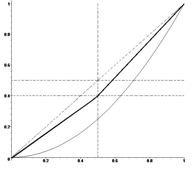
Refer to caption
Figure 4. The function ff.

Observe that ff is a bijection from [0,1][0,1] onto [0,1][0,1] and that for any 0<x<10<x<1 one has that

g⁡(g⁡(x))<g⁡(f⁡(x))<f⁡(f⁡(x)),g\big(g(x)\big)<g\big(f(x)\big)<f\big(f(x)\big)\,,

because gg is increasing and since for any x∈(0,1)x\in(0,1), we have g⁡(x)<f⁡(x)g(x)<f(x). In general g(n)​(x)<f(n)​(x)g^{(n)}(x)<f^{(n)}(x), for any x∈(0,1)x\in(0,1) and any integer n≥1n\geq 1.

Let α0=1/2\alpha_{0}=1/2. We define now a sequence indexed by ℤ\mathbb{Z} by αn=f(n)​(α0)\alpha_{n}=f^{(n)}(\alpha_{0}), for n≥1n\geq 1, and α−n=f−n​(α0)\alpha_{-n}=f^{-n}(\alpha_{0}), for n≥1n\geq 1. It is easy to check that

αn=12​(2​β)nand1−α−n=12​1(2−2​β)n.\alpha_{n}=\frac{1}{2}\,(2\beta)^{n}\quad\text{and}\quad 1-\alpha_{-n}=\frac{1}{2}\,\frac{1}{(2-2\beta)^{n}}.

Now, for each n≥1n\geq 1 we have

f(2​n)​([0,α−n])⊂[0,αn],f^{(2n)}\big([0,\alpha_{-n}]\big)\subset[0,\alpha_{n}]\,,

and then that

∫01f(2​n)​(t)​𝑑t\displaystyle\int_{0}^{1}f^{(2n)}(t)dt =∫0α−nf(2​n)​(t)​𝑑t+∫α−n1f(2​n)​(t)​𝑑t≤αn​α−n+(1−α−n)\displaystyle=\int_{0}^{\alpha_{-n}}f^{(2n)}(t)dt+\int_{\alpha_{-n}}^{1}f^{(2n)}(t)dt\leq\alpha_{n}\alpha_{-n}+(1-\alpha_{-n})
=12​(2​β)n​(1−12​1(2−2​β)n)+12​1(2−2​β)n≤12​(2​β)n+12​1(2−2​β)n<δn\displaystyle=\frac{1}{2}\,(2\beta)^{n}\,\Big(1-\frac{1}{2}\,\frac{1}{(2-2\beta)^{n}}\Big)+\frac{1}{2}\,\frac{1}{(2-2\beta)^{n}}\leq\frac{1}{2}\,(2\beta)^{n}+\frac{1}{2}\,\frac{1}{(2-2\beta)^{n}}<\delta^{n}

taking δ=max⁡(2​β,1/(2−2​β))\delta=\max(2\beta,1/(2-2\beta)).

ii) The case g′​(1)=1g^{\prime}(1)=1. For simplicity, we will change the roles of the points 0 and 1. So assume that g′​(0)=1g^{\prime}(0)=1 and g′​(1)=0g^{\prime}(1)=0. For some positive integer kk, and for some aa positive and small enough, we have that

g⁡(x)<x⁡(1−a​xk):=f⁡(x),for​x∈(0,1/2].g(x)<x(1-ax^{k}):=f(x),\quad\text{for}\ x\in(0,1/2]\,.

Following the argument in part i), to obtain (7.2), we just have to analyze the rate of convergence to 0 of the decreasing sequence defined by α0=1/2\alpha_{0}=1/2, and

αn=αn−1​(1−a​αn−1k),for​n≥1.\alpha_{n}=\alpha_{n-1}(1-a\alpha_{n-1}^{k})\,,\ \text{for}\ n\geq 1\,.

Now, since the sequence zn=a​αnkz_{n}=a\alpha_{n}^{k} verifies zn<zn−1​(1−zn−1)z_{n}<z_{n-1}(1-z_{n-1}), for each n≥1n\geq 1, we have that

1zn−1zn−1≥1\frac{1}{z_{n}}-\frac{1}{z_{n-1}}\geq 1

and, consequently, that zn<C/nz_{n}<{C}/{n} and that αn<C/n1/k\alpha_{n}<{C}/{n^{1/k}}, for some constant C>0C>0 and each n≥1n\geq 1. ∎

8. Comparison with (linear) limit theorems

For the sake of comparison we now recast the Weak Law of Large Numbers and the Central Limit Theorem in the framework of Theorem 7.1. We do not strive for sharp hypothesis. See, for instance, Chapter 9 of [7] and also [2].

Let 𝜸→=(γ1,…,γn)\boldsymbol{\vec{\gamma}}=(\gamma_{1},\ldots,\gamma_{n}) be a vector in ℝn\mathbb{R}^{n} with (strictly) positive coordinates. Consider the linear function(al) S𝜸→:ℝn↦ℝS_{\boldsymbol{\vec{\gamma}}}:\mathbb{R}^{n}\mapsto\mathbb{R} given by S𝜸→​(x1,…,xn)=∑j=1nγj​xjS_{\boldsymbol{\vec{\gamma}}}(x_{1},\ldots,x_{n})=\sum_{j=1}^{n}\gamma_{j}x_{j}; of course, this continuous function S𝜸→S_{\boldsymbol{\vec{\gamma}}} is not as selector.

We are interested in the asymptotic behavior of 𝐒𝜸→(N)​(X)\mathbf{S}_{\boldsymbol{\vec{\gamma}}}^{(N)}(X) as N→∞N\to\infty.

8.1. Weak law

Here we assume that ‖𝜸→‖1=1\|\boldsymbol{\vec{\gamma}}\|_{1}=1, so that S𝜸→S_{\boldsymbol{\vec{\gamma}}} is an average. Observe that ‖𝜸→‖2<1\|\boldsymbol{\vec{\gamma}}\|_{2}<1.

Assume that XX has finite variance σ2\sigma^{2} and expectation μ\mu. Observe that 𝐒𝜸→​(X)\mathbf{S}_{\boldsymbol{\vec{\gamma}}}(X) has variance ‖𝜸→‖22​σ2\|\boldsymbol{\vec{\gamma}}\|_{2}^{2}\,\sigma^{2} and expectation μ\mu. In general, 𝐒𝜸→(N)​(X)\mathbf{S}_{\boldsymbol{\vec{\gamma}}}^{(N)}(X) has variance ‖𝜸→‖22​N​σ2\|\boldsymbol{\vec{\gamma}}\|_{2}^{2N}\sigma^{2} and expectation μ\mu. We conclude, since ‖𝜸→‖2<1\|\boldsymbol{\vec{\gamma}}\|_{2}<1, that

𝐒𝜸→(N)​(X)​⟶dN→∞​μ.\mathbf{S}_{\boldsymbol{\vec{\gamma}}}^{(N)}(X)\underset{N\to\infty}{\stackrel{{\scriptstyle\rm d}}{{\longrightarrow}}}\mu\,.

This is, of course, a rephrasing (of some form) of the Weak Law of Large Numbers.

Observe that, since the variance of 𝐒𝜸→​(X)\mathbf{S}_{\boldsymbol{\vec{\gamma}}}(X) is ‖𝜸→‖22​σ2\|\boldsymbol{\vec{\gamma}}\|_{2}^{2}\,\sigma^{2} and ‖𝜸→‖22<1\|\boldsymbol{\vec{\gamma}}\|_{2}^{2}<1, the only variables XX (with finite variance) such that 𝐒𝜸→​(X)=dX\mathbf{S}_{\boldsymbol{\vec{\gamma}}}(X)\stackrel{{\scriptstyle\rm d}}{{=}}X are the constants. Compare with Remark 7.2.

More generally, let 𝜸→(k)\boldsymbol{\vec{\gamma}}^{(k)}, k≥1k\geq 1, be a sequence of vectors in ℝn\mathbb{R}^{n} with positive coordinates and such that ‖𝜸→(k)‖1=1\|\boldsymbol{\vec{\gamma}}^{(k)}\|_{1}=1 for k≥1k\geq 1. For such a sequence we have that, if ∑k=1∞(1−‖𝜸→(k)‖2)=+∞\sum_{k=1}^{\infty}(1-\|\boldsymbol{\vec{\gamma}}^{(k)}\|_{2})=+\infty, then for any random variable XX with finite variance,

(𝐒𝜸→(N)∘𝐒𝜸→(N−1)∘⋅∘𝐒𝜸→(1))(X)⟶dN→∞𝐄(X).\big(\mathbf{S}_{\boldsymbol{\vec{\gamma}}^{(N)}}\circ\mathbf{S}_{\boldsymbol{\vec{\gamma}}^{(N-1)}}\circ\cdot\circ\mathbf{S}_{\boldsymbol{\vec{\gamma}}^{(1)}}\big)(X)\underset{N\to\infty}{\stackrel{{\scriptstyle\rm d}}{{\longrightarrow}}}\mathbf{E}(X)\,.

Observe that if ∑k=1∞(1−‖𝜸→(k)‖2)<+∞\sum_{k=1}^{\infty}(1-\|\boldsymbol{\vec{\gamma}}^{(k)}\|_{2})<+\infty, the limit of (𝐒𝜸→(N)∘𝐒𝜸→(N−1)∘⋅∘𝐒𝜸→(1))(X)\big(\mathbf{S}_{\boldsymbol{\vec{\gamma}}^{(N)}}\circ\mathbf{S}_{\boldsymbol{\vec{\gamma}}^{(N-1)}}\circ\cdot\circ\mathbf{S}_{\boldsymbol{\vec{\gamma}}^{(1)}}\big)(X), if it exists, will not be a constant (unless XX itself is a constant).

8.2. Central limit

Now we assume that ‖𝜸→‖2=1\|\boldsymbol{\vec{\gamma}}\|_{2}=1. Observe that ‖𝜸→‖3<1\|\boldsymbol{\vec{\gamma}}\|_{3}<1.

Let XX be a random variable with 𝐄⁡(X)=0\mathbf{E}(X)=0, 𝐄⁡(X2)=1\mathbf{E}(X^{2})=1 and 𝐄⁡(|X|3)=ρ<+∞\mathbf{E}(|X|^{3})=\rho<+\infty. The Berry–Esseen inequality gives that

|F𝐒𝜸→​(X)​(x)−Φ⁡(x)|≤ρ​‖𝜸→‖33,for any x∈ℝ.|F_{\mathbf{S}_{\boldsymbol{\vec{\gamma}}}(X)}(x)-\Phi(x)|\leq\rho\|\boldsymbol{\vec{\gamma}}\|^{3}_{3}\,,\quad\mbox{for any $x\in\mathbb{R}$}\,.

Since 𝐒𝜸→(N)\mathbf{S}_{\boldsymbol{\vec{\gamma}}}^{(N)} is also a 𝐒\mathbf{S} operator but with the vector {(γi1,…,γiN);1≤ij≤n,1≤j≤N}\{\big(\gamma_{i_{1}},\dots,\gamma_{i_{N}}\big);1\leq i_{j}\leq n,1\leq j\leq N\} instead of the original {γi;1≤i≤n}\{\gamma_{i};1\leq i\leq n\}, it follows that for any N≥1N\geq 1,

|F𝐒𝜸→(N)​(X)​(x)−Φ⁡(x)|≤ρ​‖𝜸→‖33​N,for any x∈ℝ.|F_{\mathbf{S}_{\boldsymbol{\vec{\gamma}}}^{(N)}(X)}(x)-\Phi(x)|\leq\rho\|\boldsymbol{\vec{\gamma}}\|^{3N}_{3}\,,\quad\mbox{for any $x\in\mathbb{R}$}\,.

Since ‖𝜸→‖3<1\|\boldsymbol{\vec{\gamma}}\|_{3}<1, we conclude that

𝐒𝜸→(N)​(X)​⟶dN→∞​standard normal;\mathbf{S}_{\boldsymbol{\vec{\gamma}}}^{(N)}(X)\underset{N\to\infty}{\stackrel{{\scriptstyle\rm d}}{{\longrightarrow}}}\mbox{standard normal}\,;

again, a rephrasing of (some form) of the Central Limit Theorem.

Observe that as a consequence of this limit theorem it follows that if XX has 𝐄⁡(X)=0\mathbf{E}(X)=0, 𝐄⁡(X2)=1\mathbf{E}(X^{2})=1 (and 𝐄⁡(|X|3)<+∞\mathbf{E}(|X|^{3})<+\infty) and if XX is a fixed point of 𝐒𝜸→\mathbf{S}_{\boldsymbol{\vec{\gamma}}}, in the sense that 𝐒𝜸→​(X)=dX\mathbf{S}_{\boldsymbol{\vec{\gamma}}}(X)\stackrel{{\scriptstyle\rm d}}{{=}}X, then XX is a standard normal variable. Compare with Remark 7.2.

More generally, let 𝜸→(k)\boldsymbol{\vec{\gamma}}^{(k)}, k≥1k\geq 1, be a sequence of vectors in ℝn\mathbb{R}^{n} with positive coordinates and such that ‖𝜸→(k)‖2=1\|\boldsymbol{\vec{\gamma}}^{(k)}\|_{2}=1 for k≥1k\geq 1. For such a sequence we have that if ∑k=1∞(1−‖𝜸→(k)‖3)=+∞\sum_{k=1}^{\infty}(1-\|\boldsymbol{\vec{\gamma}}^{(k)}\|_{3})=+\infty then for any random variable XX with 𝐄⁡(X)=0\mathbf{E}(X)=0, 𝐄⁡(X2)=1\mathbf{E}(X^{2})=1 and 𝐄⁡(|X|3)=ρ<+∞\mathbf{E}(|X|^{3})=\rho<+\infty the following convergence holds

(𝐒𝜸→(N)∘𝐒𝜸→(N−1)∘⋅∘𝐒𝜸→(1))(X)⟶dN→∞standard normal.\big(\mathbf{S}_{\boldsymbol{\vec{\gamma}}^{(N)}}\circ\mathbf{S}_{\boldsymbol{\vec{\gamma}}^{(N-1)}}\circ\cdot\circ\mathbf{S}_{\boldsymbol{\vec{\gamma}}^{(1)}}\big)(X)\underset{N\to\infty}{\stackrel{{\scriptstyle\rm d}}{{\longrightarrow}}}\mbox{standard normal}\,.

References

  • [1] Alon, N. and Spencer, J. H.: The probabilistic method. Second edition. Wiley-Interscience Series in Discrete Mathematics and Optimization, Wiley-Interscience, New York, 2000.
  • [2] Anshelevich, M.: The linearization of the central limit operator in free probability theory. Probab. Theory Related Fields 115 (1999), 401–416.
  • [3] Alam, K.: Unimodality of the distribution of an order statistic. Ann. Math. Stat. 43 (1972), no. 6, 2041–2044.
  • [4] Ben-Or, M. and Linial, N.: Collective coin flipping. In Randomness and Computation, 91–115. Academic Press, New York, 1989.
  • [5] Binmore, K.: Fun and games. A text on game theory. Houghton Mifflin, 1991.
  • [6] Bollobás, B.: Combinatorics: Set systems, hypergraphs, families of vectors and combinatorial probability. Cambridge University Press, 1986.
  • [7] Breiman, L.: Probability. Classics in Applied Mathematics 7, SIAM, 1992.
  • [8] David, H. A. and Nagaraja, N. H.: Order statistics, 3d edition. Wiley, 2003.
  • [9] Eccles, T.: A stability result for the union-closed size problem. ArXiv 1311.2298, 2013.
  • [10] Embrechts, P. and Hofert, M.: A note on generalized inverses. Math. Meth. Oper. Res. 77 (2013), no. 3, 423–432.
  • [11] Engel, K.: Sperner theory. Encyclopaedia of Mathematics and its Applications 65, Cambridge Univ. Press, 1997.
  • [12] Kahn, J. and Kalai, G.: Thresholds and expectation thresholds. Comb. Prob. Comput. 16 (2007), no. 3, 495–502.
  • [13] Katona, G. O. H. : A theorem on finite sets. In Theory of Graphs, 187–207. Akadémiai Kiadé, Budapest, 1968.
  • [14] Kruskal, J. B.: The number of simplices in a complex. In Mathematical Optimization Techniques, 251–278. University of California Press, Berkeley, 1963.
  • [15] Qian, W. and Riedel, M. D.: The synthesis of Stochastic Logic to perform multivariate polynomial arithmetic. International Workshop on Logic and Synthesis, Lake Tahoe, CA, 2008.
  • [16] Li, X., Qian, W., Riedel, M., Bazargan, K. and Lilja, D.: A reconfigurable stochastic architecture for highly reliable computing. In ACM Great Lakes Symposium on VLSI, 315–320. ACM, Boston, Ma, 2009.
  • [17] Qian, W., Riedel, M. D. and Rosenberg, I.: Uniform approximation and Bernstein polynomials with coefficients in the unit interval. European J. Combin. 32 (2011), 440–463.
  • [18] Russo, L.: On the critical percolation probabilities. Z. Wahrsch. Verw. Geb. 56 (1981), 229–237.
  • [19] Zermelo, E.: Über eine Anwendung der Mengenlehre auf die Theorie des Schachspiels. In Proc. Fifth Congress Mathematicians (Cambridge 1912), 501–504. Cambridge University Press, 1913.

Francisco Durango: Departamento de Matemáticas, Universidad Autónoma de Madrid, 28049-Madrid, Spain. fra.durango@estudiante.uam.es

José L. Fernández: Departamento de Matemáticas, Universidad Autónoma de Madrid, 28049-Madrid, Spain. joseluis.fernandez@uam.es

Pablo Fernández: Departamento de Matemáticas, Universidad Autónoma de Madrid, 28049-Madrid, Spain. pablo.fernandez@uam.es

María J. González: Departamento de Matemáticas, Universidad de Cádiz, 11510-Puerto Real, Cádiz, Spain. majose.gonzalez@uca.es