Casimir Energies of Periodic Dielectric Gratings

The Casimir force, arising from fluctuations of charges and fields in quantum electrodynamics, has entered an era of unprecedented precision measurements. One particularly appealing application is to the case of periodic gratings, where both lateral and perpendicular forces can be measured [1, 2, 3, 4, 5]. On the theoretical side, one can use Rayleigh expansion methods for rectangular [6] and lamellar [7, 8, 9] gratings, $C$ methods [10], and perturbative methods [11, 12, 13] to calculate Casimir interaction energies of periodic dielectrics or conductors. These approaches are often limited in their ability to handle deep corrugations [14, 15, 16, 17, 18, 19, 20] (for perfectly conducting rectangular corrugations, one can obtain exact results using path integral techniques [21, 22]). Here we take a different approach and model the grating as a smooth dielectric function that depends on $z$, the distance perpendicular to the grating, is periodic with period $L$ in the transverse direction $x$, and is independent of the transverse direction $y$. The dielectric function can also depend on frequency, including dissipation (e.g. a Drude model). We will use scattering theory methods [23, 24, 25, 26, 27, 28, 29, 30] to find the Casimir energy for two such gratings in terms of the reflection matrix for scattering from each grating individually. We compute these reflection matrices using a variable phase approach [31, 32], which enables us to solve the scattering theory problem by integrating an ordinary matrix differential equation in $z$ for the coupled modes arising from a Fourier decomposition in $x$. This calculation is the Cartesian analog of the approach in Ref. [33], which shows how to obtain scattering matrices of asymmetric objects by solving coupled ordinary differential equations in a spherical basis. For the grating case, the band structure in the periodic direction leads to a discrete scattering problem, since mixing only takes place between modes whose wave numbers in the $x$ direction differ by an integer multiple of $\frac{2\pi}{L}$. Because the method obtains the full $S$-matrix without approximation, it can be applied to an arbitrary background profile, limited only by the computational resources needed to describe the Fourier decomposition of the dielectric background.

In the next section, we show how to compute the electromagnetic reflection matrices for scattering from a periodic dielectric using the generalized variable phase method. Then, in the following section, we demonstrate the method by using this scattering data to carry out a sample calculation of the Casimir interaction energy of two dielectric gratings.

We formulate the problem as Maxwell scattering from a periodic, frequency- and space-dependent dielectric $\epsilon(k,\bm{r})$,

where $\omega=ck$ is the wave frequency. This equation has transverse solutions with $k\neq 0$, as well as unphysical longitudinal solutions with $k=0$. We use the technique of Ref. [33], in which we instead solve the generalized Helmholtz equation

Eq. (2) shares the same transverse solutions as Eq. (1), but it has longitudinal solutions for which $k$ is related to wavelength and frequency in the usual way, rather than having $k=0$. Our method will include these longitudinal modes in the calculation, so that we are working with a nonsingular differential operator. We then discard the longitudinal modes at the end of the calculation via projection onto the subspace of transverse modes.

We consider the case where $\epsilon(k,\bm{r})$ is periodic in the $x$ direction with period $L$ and independent of $y$. (It is straightforward to extend this formalism to the case where $\epsilon(k,\bm{r})$ is periodic in both the $x$ and $y$ directions.) As a result, we can write $\epsilon(k,\bm{r})$ as a Fourier series,

where $\epsilon_{n}(k,z)\to\delta_{n0}$ for $z\to\pm\infty$. For simplicity, we also assume that $\epsilon(k,\bm{r})$ is symmetric in $z$. We can then write the general solution to Eq. (2) as

where we have decomposed the solutions in terms of the transverse momenta $k_{x}$ and $k_{y}$, the vector component $i=x,y,z$, and the parity under $z$ reflection $\chi=\pm 1$.

Because the dielectric background is periodic in $x$ and independent of $y$, the only values of $k_{x}$ that mix are those differing by integer multiples of $\frac{2\pi}{L}$, while the $k_{y}$ values do not mix at all. The result is a band structure in $k_{x}$ where each scattering channel is labeled by $k_{x_{0}}$ ranging from $-\frac{\pi}{L}$ to $\frac{\pi}{L}$ and comprises a discrete set of $k_{x}$ values, differing from $k_{x_{0}}$ by an integer times $\frac{2\pi}{L}$. We therefore solve a matrix scattering problem for modes with $k_{x}=k_{x_{0}}+\frac{2\pi n}{L}$, indexed by the integer $n$, and a fixed value of $k_{y}=k_{y_{0}}$. We define $k_{z}=k\sqrt{1-\frac{k_{x}^{2}+k_{y}^{2}}{k^{2}}}$, and each mode has three spatial components since we have a vector field. For a given $k$ and $\chi$, we obtain a separate matrix scattering problem for each value of $k_{x_{0}}$ between $-\frac{\pi}{L}$ and $\frac{\pi}{L}$ and each value of $k_{y_{0}}$ from zero to infinity. On the real $k$-axis, this matrix is finite-dimensional, since only modes with $|n|<\frac{L}{2\pi}\left(|k|-\sqrt{k_{x_{0}}^{2}+k_{y_{0}}^{2}}\right)$, those that represent propagating rather than evanescent waves, contribute to the $S$-matrix. To compute the Casimir energy, we will analytically continue to the imaginary $k$-axis, in which case there will be no limit on $|n|$; as usual, we will be able to truncate these matrices at large wave number for numerical calculations. Even though the ultimate calculation will be carried out on the imaginary axis, it is helpful to begin from the real axis, because there the unitarity of the finite-dimensional $S$-matrix gives a strong check of the numerical calculation.

In the region where the dielectric differs from vacuum, the decomposition of scattering solutions into transverse and longitudinal components is highly nontrivial. The $S$-matrix, however, is defined in terms of free asymptotic waves, for which it is straightforward to identify transverse and longitudinal modes. We have the TE and TM transverse modes respectively,

and the longitudinal mode

where $\bm{k}=(k_{x},k_{y},k_{z})$ and $k=|\bm{k}|$. The $S$-matrix for scattering governed by Eq. (2) must commute with the projection onto the subspace of transverse modes (for both real and imaginary wave number), which gives another strong check on our numerical calculations.

To define the $S$-matrix, we combine the solutions with $k$ and $-k$ (or, equivalently, the outgoing wave solution and its conjugate, the incoming wave solution) to form the physical wave functions [34] in the symmetric and antisymmetric channels under reflection in $z$,

respectively, where $F(k,k_{x_{0}},k_{y_{0}},z)$ is the outgoing wave solution, written as a matrix in the vectorspace of modes with $k_{x}=k_{x_{0}}+\frac{2\pi n}{L}$ and $k_{y}=k_{y_{0}}$. Here $\hat{M}$ is a diagonal matrix with $+1$ on the diagonal for $x$ and $y$ vector components and $-1$ for $z$ components. This matrix captures the additional minus sign involved in imposing the parity boundary conditions on the $z$-component of the vector wave function at $z=0$. On the real axis, the resulting $\hat{S}$ matrix is unitary and finite-dimensional: it only involves asymptotic propagating waves with $|n|<\frac{L}{2\pi}\left(|k|-\sqrt{k_{x_{0}}^{2}+k_{y_{0}}^{2}}\right)$.

To compute the $S$-matrix, we consider both the regular and outgoing solutions to the generalized Helmholtz equation in Eq. (2). In doing so, it will be helpful to parameterize these solutions in a way that factors out the free solutions [35]. Defining $\hat{k}_{z}(k,k_{x_{0}},k_{y_{0}})$ to be a diagonal matrix with $k_{z}$ on the diagonal, we write the outgoing solution as

and the transpose of the regular solution as (note the reversed order)

The regular solution is different in the two parity channels, but the outgoing solution is the same. Plugging these solutions into Eq. (2), we obtain equations of the form [33]

and

which are to be solved subject to the boundary conditions

and

where $\hat{h}_{+}(k,k_{x_{0}},k_{y_{0}})$ is a diagonal matrix whose diagonal entries are zero for the $z$ components of $E_{i,\chi,k_{x},k_{y}}(z)$ and $(-ik_{z})^{-1}$ for the $x$ and $y$ components, while $\hat{h}_{-}(k,k_{x_{0}},k_{y_{0}})$ is a diagonal matrix whose diagonal entries are zero for the $x$ and $y$ components of $E_{i,\chi,k_{x},k_{y}}(z)$ and $(-ik_{z})^{-1}$ for the $z$ components. The matrices $\hat{D}_{0}(k,k_{x_{0}},k_{y_{0}},z)$ and $\hat{D}_{1}(k,k_{x_{0}},k_{y_{0}},z)$ are the result of applying the vector derivatives in Eq. (2) to the general solution in Eq. (4) and depend on the dielectric Fourier components $\epsilon_{n}(k,z)$ and their derivatives. These matrices are typically obtained from symbolic computation, as shown in a sample calculation available from http://community.middlebury.edu/˜ngraham .

The $S$-matrix is then given by [34, 33]

where $\widetilde{\cal W}_{\pm}(k,k_{x_{0}},k_{y_{0}})$ is the generalized Wronskian of the incoming and outgoing solutions,

which is independent of $z$. Here $\hat{N}(k,k_{x_{0}},k_{y_{0}})$ is a diagonal matrix with $\sqrt{\frac{k}{k_{z}}}$ on the diagonal, which normalizes the incident flux in the different components of our scattering basis, yielding a unitary $S$-matrix for real $k$. Since the Wronskian can be evaluated at any value of $z$, in order to optimize the numerical calculation, we will choose a common fitting point at the characteristic width of the potential, and then evaluate the Wronskian by integrating $\hat{G}$ inward to this point from infinity and $\hat{H}_{\pm}$ outward to this point from the origin. The numerical advantages of this approach become particularly important for imaginary $k$, as will be required for our Casimir energy calculation. Although in principle the $S$-matrix could be obtained from either $\hat{G}$ or $\hat{H}_{\pm}$ alone, this combined approach is necessary on the imaginary $k$-axis to avoid numerical problems from growing exponentials in that case.

With the $S$-matrix in hand, we are prepared to consider the Casimir energy. For two gratings whose origins are separated by the vector $\Delta\bm{r}$, we define the translation matrix $\hat{U}(k,k_{x_{0}},k_{y_{0}})$ as a diagonal matrix with $\exp[i\bm{k}\cdot\Delta\bm{r}]$ on the diagonal. For each grating, we form the reflection coefficient as the difference between the $S$-matrices for the symmetric and antisymmetric channels,

We then project both $\hat{U}(k,k_{x_{0}},k_{y_{0}})$ and $\hat{r}(k,k_{x_{0}},k_{y_{0}})$ onto the subspace spanned by the transverse modes in Eq. (5), denoting the results as $\bar{U}(k,k_{x_{0}},k_{y_{0}})$ and $\bar{r}(k,k_{x_{0}},k_{y_{0}})$ respectively. This projection discards the longitudinal modes, leaving the transverse modes unchanged.

The Casimir interaction energy per unit area for two identical gratings is then given by the scattering theory approach as [23, 24, 26, 27, 28, 29, 30]

This result is now suitable for numerical computation.

We illustrate the method by calculating the Casimir force between two identical gratings with a frequency-independent dielectric function given in terms of Fourier components

with all other $\epsilon_{n}(k,z)=0$. This profile gives a step function shape in $z$; we choose height $h=2$, width $w=2\ell_{0}$, steepness $s=16/\ell_{0}$, and period $L=2\pi\ell_{0}$, where we work in units of the length $\ell_{0}$. The total dielectric function is shown in Fig. 1.

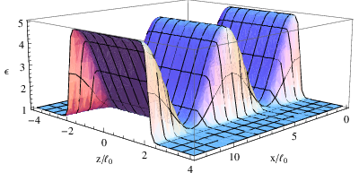
We let $\Delta z$ be the separation between the gratings, measured between their center planes, and $\Delta x$ be their transverse displacement.

To see the effects of corrugations on the Casimir force, we compare the Casimir energy of the two gratings to the Casimir energy of two planar dielectric slabs with the same transverse area, maximum width $2w$, and dielectric constant $\epsilon=2h$. For a slab, the reflection matrix is diagonal, with diagonal entries given by the Fresnel result

for the TE and TM polarization modes respectively, where

the incident and transmitted angles are given by

and $\beta=k\sqrt{\epsilon}\cos\phi_{t}$. Results for the ratio of Casimir energies $\frac{{\cal E}}{{\cal E}_{\hbox{\tiny slab}}}$ are shown in Fig. 2. In this calculation, the $\kappa$ and $k_{y_{0}}$ integrals in Eq. (21) are truncated at $k_{\hbox{\tiny min}}=0.0078125/\ell_{0}$ and $k_{\hbox{\tiny max}}=2.5/\ell_{0}$, and the matrices in $k_{x}$ are truncated to include only modes within the same $k_{\hbox{\tiny max}}$ of $k_{x_{0}}$. For each $\kappa$, $k_{x_{0}}$, and $k_{y_{0}}$, for both $\kappa$ and $-\kappa$ we integrate $\hat{G}$ and $\hat{H}_{\pm}$ from $z=0$ and $z=4w$ respectively to a common fitting point at $z=w$. We form the Wronskian in the symmetric and antisymmetric channels to obtain the $S$-matrices in each channel, which we then combine to form the reflection matrix. Because of the symmetry of our dielectric profile, the integrand is even in $k_{x_{0}}$ and we only need to compute the case of positive $k_{x_{0}}$.

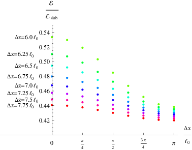
As we expect, Fig. 2 shows that the energy of the two gratings is smaller in magnitude than in the case of two slabs, since we have effectively removed dielectric material from the slabs to form the gratings. The dependence of the energy of the gratings on $\Delta x$ leads to a lateral force trying to align the gratings (the energy for the case of two slabs is negative and independent of $\Delta x$). The dependence on $\Delta x$ becomes weaker as $\Delta z$ increases, since the calculation is increasingly dominated by long wavelength fluctuations, which are less sensitive to the contours of the grating.

Having demonstrated the effectiveness of this method with a sample calculation, a natural next step is to develop large-scale numerical calculations, which can allow for closer separations by handling a larger range of $k$ values, and can also include more Fourier components in the dielectric function in order to focus on steep gratings, for which calculations based on the Rayleigh expansion are often not applicable. Work in this direction is in progress [36].