Discrete Renormalization Group for Tensorial Group Field Theory
Abstract
This article provides a Wilsonian description of the perturbatively renormalizable Tensorial Group Field Theory introduced in arXiv:1303.6772 [hep-th] (Commun. Math. Phys. 330, 581-637). It is a rank-3 model based on the gauge group , and as such is expected to be related to Euclidean quantum gravity in three dimensions. By means of a power-counting argument, we introduce a notion of dimensionality of the free parameters defining the action. General flow equations for the dimensionless bare coupling constants can then be derived, in terms of a discretely varying cut-off, and in which all the so-called melonic Feynman diagrams contribute. Linearizing around the Gaussian fixed point allows to recover the splitting between relevant, irrelevant, and marginal coupling constants. Pushing the perturbative expansion to second order for the marginal parameters, we are able to determine their behaviour in the vicinity of the Gaussian fixed point. Along the way, several technical tools are reviewed, including a discussion of combinatorial factors and of the Laplace approximation, which reduces the evaluation of the amplitudes in the UV limit to that of Gaussian integrals.
1 Introduction
Group Field Theory (GFT) [1, 2, 3, 4] is an approach to Quantum Gravity which lies at the crossroad of Tensor Models [5, 6, 7, 8, 9], Loop Quantum Gravity (LQG) [10, 11, 12, 13, 14], and Spin Foam Models [15, 16, 17, 18]. This research program aims at addressing questions which are notoriously difficult in loop quantum gravity, such as the construction of the dynamical sector of the theory and of its continuum limit [19], by means of quantum and statistical field theory techniques. A GFT is nothing but a field theory defined on a (compact) group manifold, with specific non-local interactions. The latter are chosen in such a way that the Feynman expansion generates cell complexes of a given dimension, interpreted as discrete space-time histories. In particular, the amplitudes of any spin foam model can be generated by a suitably constructed GFT, which is what triggered interest in the GFT formalism [20, 21]. Hence GFTs can be viewed as a natural way of completing the definition of spin foam models, which by themselves do not associate unambiguous amplitudes to boundary states. Note that alternatively to the summing strategy implemented in GFT, one can instead look for a definition of the refinement limit of spin foams [22, 23, 24]. A more direct route from canonical LQG to GFT has recently been proposed [25]: from this perspective, the GFT formalism defines a second-quantized version of LQG, and hence should be especially relevant to the analysis of the many-body sector of the theory (see [26, 27] for cosmological applications of these ideas).
Thanks to recent breakthroughs in the field of tensor models, triggered by the pioneering work of Gurau [28], who found a generalization of the expansion of matrix models [29, 30, 31], standard field theory techniques are currently being developed and generalized to more and more complicated GFTs. The common ingredient to all the models studied so far is tensor invariance [32, 33, 34, 9, 35, 36]: it provides a generalized notion of locality for GFTs, which as we have just mentioned are non-local in the ordinary sense. They then differ by: the rank of the tensor fields, identified with the space-time dimension; the space in which the indices of the tensor fields live; and the propagator. Theories based on tensors with indices in the integers11 1 Equivalently, such models can also be viewed as GFTs on the group . and trivial propagator are referred to as Tensor Models. A wealth of results about their expansions has now been accumulated [37, 38, 39, 40, 41], from single to multiple scalings in [42, 43, 44], and up to the rigorous non-perturbative level [45, 46]. Similar models with non-trivial propagators are referred to as Tensorial Field Theories [47, 48, 49, 50]: they are indeed genuine field theories, for which full-fledge renormalization methods take over the large expansion. Finally, Tensorial Group Field Theories (TGFT) are Tensorial Field Theories based on (compact) Lie groups22 2 In view of the correspondence between simple GFTs and tensor models resulting from harmonic analysis, we have in mind a theory in which the group structure plays a significant enough role.. The only models of this type available in the literature so far are the so-called TGFTs with gauge invariance condition [51, 52, 53, 54]. This paper will focus on one such example, a rank- renormalizable model based on the gauge group . In addition to being technically relevant to spin foam models and LQG in general, it is expected to be related to Euclidean quantum gravity in three dimensions, though the full correspondence is unclear at present: while tensor invariance seems to provide a perfectly viable discretization prescription, the quantum gravity interpretation (if any) of the Laplace-type propagator has not been investigated in details.
The aim of this article is two-folds. The first objective is to pave the way towards general renormalization group techniques à la Wilson, which will allow to better understand the theory spaces of TGFTs, their flows and fixed points. Secondly, we want to determine the properties of the Gaussian fixed point of the specific model we are considering. Indeed, the examples worked out so far [55, 56] suggest that asymptotic freedom might be a reasonably generic property of Tensorial Field Theories. The occurrence of asymptotic freedom in such models is surprising at first, because they are not gauge theories. However, the non-locality of the interactions is responsible for wave-function renormalization terms which are absent from ordinary scalar field theories, and which typically dominate over the coupling constants renormalization terms. Hence the -functions can be negative despite the absence of non-Abelian gauge symmetries.
In section 2, we introduce the model and the main results of [52] which are relevant to the present publication. In addition, we provide a detailed analysis of the symmetry factors appearing in the Feynman expansion, which significantly simplifies the calculations reported on in the later sections. In section 3 we introduce a discrete version of Wilson’s renormalization group. It is based on the introduction of dimensionless coupling parameters, and differs in this sense from the analyses performed in previous works [55, 56, 52]. A new notion of reducibility is also proposed, which is to some extent the correct generalization of -particle reducibility from ordinary local field theories to TGFTs. In section 4, we linearize the flow equations in the vicinity of the Gaussian fixed point. This allows to classify the coupling constants in terms of their relevance, and recover the fact that this model is renormalizable up to order six interactions. We then explicitly compute the eigendirections associated to this linear system, and deduce the functional relationship between the marginal coupling constants and the other renormalizable constants in the asymptotic UV region. In section 5, the flow equations for the marginal coupling constants are pushed to second order in perturbation theory. Although the calculations underlying the results of this section are rather lengthy and technical, they are as far as we know the first of their kind in a non-Abelian model and are therefore included in full details. Finally, the qualitative properties of the flow equations in the vicinity of the Gaussian fixed point are investigated in section 6. Relying on a continuous version of the discrete flow, we will be able to completely settle the question of asymptotic freedom when and have same signs, and in particular when they are strictly positive.
2 The model and its divergences
In this section, we introduce the TGFT model studied in [52], and summarize some of the key steps in the proof of its renormalizability. This paper was to a large extent based on a Bogolioubov recursion relation, which defined the renormalized series. The analysis was greatly simplified, thanks to a refined notion of graph connectedness, called face-connectedness. As already noted in [52], this structure is not appropriate in the effective Wilsonian language, where connected graphs in the ordinary sense33 3 This ordinary notion was called vertex-connectedness in [52]. must be summed over. Since the purpose of this paper is to investigate further the renormalization group flow equations of this model, we will only outline the definition of the effective series, in which the usual graph-theoretic notion of connectedness is at play.
2.1 Definition and Feynman expansion
We are interested in a group field theory for a field and its complex conjugate . The free theory is defined by a Gaussian measure , with covariance , that is to say:
| (1) |
This covariance can be perturbed by non-Gaussian interaction terms, encapsulated in an action , so as to define the (Euclidean) interacting partition function:
| (2) |
In tensorial GFTs, is assumed to be a weighted sum of connected tensor invariants. By analogy with space-time based quantum field theories, this prescription is referred to as a locality principle, and is used as such for renormalization purposes. Connected tensor invariants in dimension are in one-to-one correspondence with -colored graphs (also called -bubbles), which are bipartite edge-colored closed graphs with fixed valency at each node. In our -dimensional context, a -colored graph is a connected graph with two types of nodes (black or white), and edges labeled by integers (the colors), in such a way that: a) any edge connects a white node to a black one; b) at any node, exactly three edges with distinct colors meet. Simple examples are provided in Figure 1.

The unique invariant associated to a given -bubble is constructed as follows: a) each white (resp. black) node represents a field (resp. a conjugate field ); b) a color- edge between the nodes and indicates a convolution with respect to the variables of the fields located at and respectively.
Example. The colored graph on the right side of Figure 1 represents the following invariant integral:
| (3) |
With these definitions, the interaction part of the action can be written as
| (4) |
where is the set of all bubbles, and is the coupling constant associated to . In order to simplify the counting of Feynman graphs, we divided each coupling constant by a combinatorial factor , defined as the number of automorphisms of the bubble graph .
Definition 1.
Let be a colored graph. An automorphism of is a permutation of its nodes44 4 This definition coincides with the more general concept of graph automorphism, even if a graph automorphism is usually thought of as a couple of permutations, respectively of the nodes and of the edges. When imposing compatibility with the colored structure, becomes redundant, hence our definition in terms of a single permutation., such that:
- (i)
conserves the nature of the nodes;
- (ii)
if and are connected by an edge of color , then so do and .
At this stage, it is natural to assume that the colors have no physical role other than imposing combinatorial restrictions on the interactions, and we will therefore require to be invariant under color permutations. This can be formalized as follows. The group of permutations of the color set acts naturally on : for any , is the bubble obtained from by permutation of the color labels as dictated by . The invariance of under color permutation is simply the statement that:
| (5) |
The second ingredient of the model is the covariance . In [51, 52], it was motivated from two basic requirements: first, it should impose the so-called gauge invariance condition of spin foam models; second, it should have a rich enough spectrum so as to provide an abstract notion of scale. The gauge invariance condition is an invariance of the field55 5 Note that there is no gauge symmetry involved at the field theory level, and that the nomenclature arises from the lattice gauge theory interpretation of the amplitudes. under an arbitrary simultaneous translation of its variables:
| (6) |
In the GFT context we can however work with generic fields, and impose (6) through the covariance. The latter should therefore contain the projector on the space of gauge invariant fields, defined by the kernel:
| (7) |
In order to get a non-trivial spectrum, we combine it with the operator
| (8) |
where denotes the Laplace operator on acting on the color- variables. At this stage, this should be seen as a conservative natural choice, partially motivated by a study of the -point radiative corrections of the Boulatov-Ooguri models [57], and formal analogies with the Osterwalder-Schrader axioms [9, 35]. The covariance is then defined as66 6 It is easily seen that and commute.
| (9) |
whose kernel can be written in the Schwinger representation:
| (10) |
where is the heat kernel on at time . This covariance is ill-defined at coinciding points , and this can be regulated by cutting-off the contribution of the integral over in the neighborhood of . The divergences in this cut-off, generic in the perturbation expansion of the theory, can be analyzed in details.
The unnormalized -point functions can be expanded perturbatively in terms of Feynman amplitudes, which are indexed by generalized -colored graphs. The new type of lines, of color and represented as dashed lines, is introduced to represent the propagators; they connect the elementary bubble vertices generated by . These lines can also appear as external legs, contrary to the internal bubble lines, and this is the only respect in which the Feynman graphs differ from generic -colored graphs. Given a Feynman graph , we define as the number of external legs, and as the number of bubble vertices of type . Then
| (11) |
where is a symmetry factor associated to , and its amplitude. A simple counting shows that is nothing but the number of automorphisms of , which generalizes the definition of for bubbles (hence the notation).
Definition 2.
Let be a Feynman graph. An automorphism of is a permutation of its nodes, such that:
- (i)
conserves the nature of the nodes;
- (ii)
if and are connected by an edge of color , then so do and ;
- (iii)
if a node (resp. ) is connected to an external leg , then (resp. ).
Proposition 1.
The symmetry factor associated to an arbitrary Feynman graph is the order of its group of automorphisms.
Proof.
Consider a Feynman graph , with labeled external legs, and bubbles of type for any . Define then the group
| (12) |
where is the permutation group of elements, and is the group of automorphisms of . Its order is
| (13) |
One can fix an arbitrary labeling of all the nodes of all the vertices appearing in . Any Wick contraction with the same vertices appearing in the Feynman expansion is then represented by a set of pairs of labels. Call the set of all possible such pairings. acts naturally on , by permutation of identical bubbles and by automorphism on each individual bubble. The Feynman graph can be identified with the orbit of some , and the stabilizer to the group of automorphisms . Taking the factors coming from the perturbative expansion of the exponentials and from the definition of the action into account, we therefore obtain:
| (14) | |||||
∎
It is immediate to remark that, because of the colored structure of the Feynman graphs, the symmetry factor of any connected and non-vacuum graph (i.e. with at least one external leg) is simply . This implies in particular that the connected and normalized Schwinger functions expand as:
| (15) |
Examples. The graphs , and represented in Figure 2 have different symmetry factors. is a connected and non-vacuum graph with external legs, hence . On the other hand, its amputated version admits one non-trivial automorphism, and therefore . Finally, the vacuum graph has a symmetry factor .


In order to write the explicit expression of , we need to introduce further graph-theoretic definitions and notations. We note the set of color- internal edges in , and the set of external legs, which we will sometimes simply call lines and legs. We can furthermore partition , where (resp. ) is the set of legs hooked to white (resp. black) nodes. A face of color is a non-empty subset which, upon addition of color- edges only, can be completed into a maximally connected subset of color- edges and (internal, color-) lines. Such a maximally connected subset may form a closed loop, we say that is internal (or closed) in this case, and is external (or open) otherwise. The set of internal faces and external faces of are respectively noted , and . We will also need to keep track of direct identifications of boundary variables through single colored lines. We call these empty external faces because they play a similar role as external faces; their set is denoted . When no confusion arises, we will use the same symbol to denote the cardinality of one of the sets defined so far and the set itself. We can fix an arbitrary orientation of the lines and faces , and encode their adjacency relations into a matrix or 0. However, in order to make the expressions more explicit, it is convenient to fix the orientations so that: a) is positively oriented from the white to the black end nodes it connects; b) if , and otherwise77 7 The fact that the faces can always be oriented in such a way is a particularity of tensorial GFTs.. This canonical orientation allows to define the source and target of an external face. The function maps to , where is the color of and is the external leg connected to its source. We define in a similar way. The bare amplitude of a graph is a function of external group elements , which formally writes:
| (16) | |||||
We clearly separated the contributions of the internal faces (first line), from the external propagators (second line88 8 We could simplify this expression by means of the symmetry , but we think that the present expression is better suited for what will come next.), and how these are connected to the holonomy variables in the bulk through the external faces (third and fourth line).
2.2 Divergences and power-counting
In [52], the scale ladder provided by the parameter was used as a basis for renormalization theory. Divergences from high scales (i.e. from the region ) generate counter-terms at lower scales (i.e. bigger parameters), and the theory is renormalizable if those can be reabsorbed into a finite number of coupling constants. The divergences can be most easily understood in the multiscale representation of the Feynman amplitudes. This consists in slicing the range of the Schwinger parameter , according to a geometric progression. To this effect, one fixes an arbitrary constant and define the propagator at scale by:
| (17) |
if and
| (18) |
This induces a decomposition of the amplitude of a graph as a sum indexed by internal scale attributions :
| (19) |
The amplitude at scale is simply obtained from (16) by restricting the integrals to the slices . Note that the external legs are left untouched, and by convention they are attributed the scale label . The sum over is regulated thanks to the introduction of a cut-off on the scale labels , which can be removed only after renormalization. The main interest of the decomposition (19) is that it allows to compute rigorous bounds on by a systematic optimization procedure, which yields simple bounds on as functions of .
Given a couple , one can construct a set of high subgraphs, defined as the maximally connected subgraphs with internal scales strictly smaller than the external scales. To this effect, let us define as the subgraph made of the lines of with scales higher or equal to . Its connected components99 9 As already mentioned before, in this paper we use the ordinary graph-theoretic notion of connectedness, which is referred to as vertex-connectedness in [52]. can be labeled , where is the number of connected components. The ’s are exactly the high subgraphs at scale : they are connected; their internal lines have scales higher or equal to ; and their external legs have scales strictly smaller than . An important property of the high subgraphs is that they form an inclusion tree. That is to say that two high subgraphs and are either line-disjoint, or one is included into the other; and furthermore all the high subgraphs are by definition included in , which is itself a high subgraph (at scale ). These high subgraphs are ultimately responsible for the nested structure of divergences, and when successively integrated out, make the coupling constants run with respect to . More precisely, only the divergent high subgraphs have to be taken into account in the renormalization group equations. They are determined by a precise power-counting theorem, and we refer the reader to [51, 52] for details. For the purpose of this paper, we only need to know that the divergent high subgraphs are characterized by the inequality , where is the superficial degree of divergence, defined as [58, 51, 52]:
| (20) |
and is the rank of the incidence matrix of . Alternatively, as proven in [52], the divergence degree can be conveniently re-expressed in terms of the numbers of -valent vertices , the number of external legs and an integer :
| (21) |
Note that in [52] the bare action was assumed to stop at -valent bubble interactions, in which case the last sum reduces to . The condition characterizes the class of melonic graphs1010 10 In this paper, we always assume . When , may also be and does not imply that is melonic., which contains the divergent graphs as a subset when for (see Table 1).
| 6 | 0 | 0 | 0 | 0 |
|---|---|---|---|---|
| 4 | 0 | 0 | 0 | 1 |
| 4 | 0 | 1 | 0 | 0 |
| 2 | 0 | 0 | 0 | 2 |
| 2 | 0 | 1 | 0 | 1 |
| 2 | 0 | 2 | 0 | 0 |
| 2 | 1 | 0 | 0 | 0 |
Let us conclude this section by recalling how melonic graphs are defined.
Definition 3.
Let be a graph. For any integer such that , a -dipole is a line of linking two nodes and which are connected by exactly additional colored lines.
Definition 4.
Let be a graph. The contraction of a -dipole is an operation consisting in:
- (i)
deleting the two nodes and linked by , together with the lines that connect them;
- (ii)
reconnecting the resulting pairs of open legs according to their colors.
We call the resulting graph.
See Figure 3 for examples of -dipoles and their contractions.

Definition 5.
We call contraction of a subgraph the successive contractions of all the lines of . The resulting graph is independent of the order in which the lines of are contracted, and is noted .
Given a graph , and some lines , we will denote by the minimal subgraph of containing the lines .
Definition 6.
A melopole is a single-vertex graph such that there is at least one ordering of its lines as such that is a -dipole for . See Figure 4.

Definition 7.
A melonic graph is a connected1111 11 This definition slightly differs from that of [52], in the sense that melonic graphs were defined to be face-connected there, which is a stronger condition. graph containing at least one maximal tree such that is a melopole.
A simple example of melonic graph is provided in Figure 5.

2.3 Contraction operators
In the multiscale representation of the amplitudes, the divergences can be extracted by the action of so-called contraction operators. In order to define them, let us introduce generalized amplitudes
| (22) | |||||
where and1212 12 For any , denotes the Lie algebra element with the smallest norm such that .
| (23) | |||||
| (24) |
We can then express any amplitude as a Taylor expansion with respect to the parameter :
| (25) | |||||
The interest of such an expression is that the remainder can be shown to be power-counting convergent [52], and can therefore be dispensed with. Moreover, one shows that
| (26) |
where are the lines of . We can therefore implicitly define the contraction operator by the equation:
| (27) |
More explicitly, the heat-kernels associated to the external faces can be integrated out, yielding:
| (28) |
Finally, if is obtain from by amputation of its external legs, we define:
| (29) |
Let us now consider higher order terms. To begin with, the first order always identically vanishes:
| (30) |
The model studied in the present paper generates quadratically divergent graphs at most, which means we will not need to go beyond second order. Moreover, all the quadratically divergent graphs have external legs and are melonic. The amplitudes we need to expand to second order have therefore the following structure:
| (31) | |||||
where has three elements. Suppose for instance that , with of color . Then on can prove that [52]:
| (32) |
where we have defined
| (33) | |||||
By use of the Leibniz rule, together with the fact that terms containing first derivatives vanish, the last two equations can be generalized to
| (34) |
where
| (35) | |||||
if there exists a of color , and
| (36) |
otherwise. Again, this definition makes no reference to external legs, and can therefore be generalized to amputated graphs: if is obtained by amputation of the external legs of , then
| (37) |
3 Renormalization group flow
In this section, we define general flow equations for Wilson’s effective action. They involve: a) a step by step integration of UV slices which retains only the tensor invariant contributions of high divergent graphs, as already outlined above; and b) a large scale approximation () of the coefficients entering the equations. Because we are working with a field theory defined on a compact group rather than Euclidean space, finite size effects make the renormalization group non-autonomous1313 13 I thank Daniele Oriti for discussions on this point. i.e. the flow equations have an explicit dependence in the cut-off. However, such effects can be neglected in the deep UV regime, where only the local structure of is probed.
3.1 Wilson’s effective action and dimensionless coupling constants
In ordinary quantum field theories, Wilson’s effective action is best described in terms of dimensionless coupling constants. In GFT, and more generally in quantum gravity, such a notion is a priori empty since all the fields and coupling constants are already strictly speaking dimensionless. Dimensionful quantities should only appear in the spectra of quantum observables such as the length, area or volume operators. For example, in canonical loop quantum gravity, the area of a surface punctured by a single spin-network link with spin is where is the (dimensionless) Immirzi parameter and is the Planck length. In this respect, the spins themselves can be attributed a canonical dimension. In our context, let us attribute a unit canonical dimension
| (38) |
to spin variables. Since the propagator decays quadratically in the spins, one immediately infers the dimension of the mass: . As for the canonical dimensions of all the other coupling constants, they can be deduced from the power-counting. For example, Table 1 shows that four-valent coupling constants will receive linearly divergent contributions of order at scale . Hence they are to be thought of as coupling constants with unit canonical dimension. More generally, we are lead in this way to define
| (39) |
for an arbitrary coupling constant , where is the valency of the bubble . Note that such a definition of canonical dimension has also recently been introduced in matrix and tensor models, for similar purposes [59]. We define the effective action at scale as a sum over all possible bubbles
| (40) | |||||
| (41) |
where (resp. ) are the dimensionful (resp. dimensionless) coupling constants. We furthermore again assume color permutation invariance, and set up . The latter is consistent provided that we allow the mass parameter of the covariance to vary with the scale. We will denote by the covariance in the slice with mass , and by the full covariance with cut-off . The dimensionless mass coupling at scale is
| (42) |
In the following, we will use perturbative expansions with respect to the dimensionless coupling constants. The degree of divergence
| (43) |
tells us how Feynman amplitudes diverge in an expansion with respect to the dimensionful parameters . Taking into account the additional scalings appearing in equation (41), we immediately infer a modified degree of divergence
| (44) |
for the new expansion in the ’s. From now on, (a non-vacuum) graph will be said to be divergent whenever , that is whenever and . The new classification of divergent graphs is summarized in Table 2.
| 6 | 0 | 0 |
| 4 | 0 | 1 |
| 2 | 0 | 2 |
3.2 Discrete renormalization group flow
In order to determine the effective action and the mass coupling from and , we proceed in two steps. The first step consists in integrating out fluctuations at scale to deduce the effective action before wave-function renormalization:
| (45) |
where the rest term is a sum of contributions which are suppressed at large , and is a possibly large constant due to vacuum divergences. contains in particular the Feynman graphs with , and the convergent Taylor remainders associated to the non-tensorial parts of the non-vacuum divergent graphs. may be written as
| (46) |
in terms of intermediate dimensionless coupling constants . The additional wave-function and mass terms
| (47) | |||||
| (48) |
respectively parameterized by a dimensionless constant and a dimension constant , are generated by the -valent divergent graphs. They need to be reabsorbed into the covariance via a field renormalization, which is the second step of the procedure. To this effect, let us define the operator
| (49) |
and call the covariance of the measure:
| (50) |
It can be computed by summing over connected -point functions, in the following way:
| (51) | |||||
The expression of is:
| (52) | |||||
the second line making the smooth cut-off on the spins explicit. Thanks to this decay we can discard the higher powers of the mass and Laplace operators generated by the exponential terms in the denominator of . Using moreover the approximation in the numerator, we are lead to:
| (53) | |||||
| (54) | |||||
| (55) |
We have thus determined the mass at scale . The other coupling constants are obtained after the field redefinition
| (56) |
The powers of subsequently appearing in the interaction part of the action must be reabsorbed into the coupling constants:
| (57) |
entering the effective action . Together with the covariance , they parameterize the theory once the cut-off has been lowered to .
3.3 Reducible graphs
In space-time based quantum field theories, momentum conservation allows to discard -particle irreducible graphs, because their contributions are strongly suppressed1414 14 They are even identically zero if one works with a sharp slicing of the momenta. when the difference between the scale of the probes and that of the internal lines grows very large. Due to the combinatorial non-locality introduced by the interactions, momentum conservation has slightly stronger implications in TGFT, which we wish to elaborate upon here.
The harmonic decomposition of the field is
| (58) |
where is the Wigner matrix associated to the irreducible representation . The full propagator 10 is diagonal with respect to the modes :
| (59) |
where
| (60) |
The kernel of a tensor invariant in this spin representation is simply a product of delta functions, identifying the indices pairwise along colored edges. As a result, these indices are conserved along the faces of the Feynman graphs. This is the counterpart of momentum conservation in local quantum field theories. Note that the key difference between these two conservation rules is of combinatorial nature, and therefore it is natural to expect that the class of graphs which are suppressed due to combinatorial obstructions in TGFTs is not exactly the same as in local quantum field theories.
Let us introduce the following notion of reducibility in TGFT.
Definition 8.
Let be a connected graph. We say that is reducible if it possesses a line which does not appear in any of the internal faces:
| (61) |
If not, is said to be irreducible.
Examples. A -particle reducible graph is always reducible, but the converse is not true (see Figure 6).


In the particular model we are considering, all divergent graphs are melonic. It turns out that -particle reducibility and reducibility are equivalent in this restricted context.
Proposition 2.
Let be a melonic graph. Then
| (62) |
Proof.
The non-trivial implication is . Let be melonic. Let us suppose that is reducible, and that is a reducible line1515 15 That is to say that verifies the condition of (61).. Then there exists a maximal tree such that is a melopole. It must be that since , being contained in no internal face, cannot form a -dipole in . Then consists in two vertices connected by , and is therefore -particle reducible. Hence is itself -particle reducible. ∎
Let us now explain why, similarly to -particle reducible graphs in ordinary field theories, the contribution of reducible graphs can be neglected in the renormalization group flow of TGFTs. Let be such a graph. Suppose moreover that the internal lines are in the slice , while the boundary data have spins in the slice . By conservation of the spins along the external faces of , the sum over the spins associated to a reducible line is effectively zero except in the region where both
| (63) |
and
| (64) |
hold. These two conditions cannot be satisfied at the same time when grows large, and therefore the amplitude of vanishes in this limit.
3.4 Melonic flow equations
Now that the general set up has been introduced, let us derive the flow equations. Given a bubble , let us note the set of melonic (one particle) irreducible graphs which give back after contraction of their internal lines. We will also note the amplitude of a graph with respect to the covariance , where is defined by , and its amputated value. The key coefficients entering the flow equations will be expressed in terms of the finite values:
| (65) |
Let be a bubble of arbitrary valency. Identifying the melonic term in appearing on the right side of equation (45), we immediately find:
| (66) | |||||
and therefore:
| (67) |
When is large enough, we can finally approximate the -dependent terms by their limit values, yielding:
| (68) |
Let us now turn to the computation of the wave-function renormalization. By color invariance, we can focus on terms proportional to at arbitrary fixed . Let us call the set of irreducible and connected -point melonic graphs. For any graph , we can define
| (69) |
Then can formally be written:
| (70) |
for any fixed .
4 Relevant and irrelevant directions around the Gaussian fixed point
In this section, we study the behavior of the model around the Gaussian fixed point:
| (71) |
4.1 Linearized flow equations
The wave function renormalization does not contribute at linear order around the Gaussian fixed point. One can also set in all the coefficients at this order.
Definition 9.
Given two bubbles , we say that is smaller than () if and only if there exists a single-vertex melonic graph on which contracts to . If in addition , we say that is strictly smaller than (). This defines a partial order relation on .
Given two bubbles such that , let us designate by the set of melonic graphs with a single bubble and which contract to . We then define the quantity
| (72) |
which is strictly positive. Let us also set for any , and for any such that the condition does not hold. The linearized flow equations around the Gaussian fixed point are:
| (73) |
4.2 Irrelevant, marginal and relevant directions
We will say that a coupling constant and its dimensionless counterpart are renormalizable if , and are non-renormalizable otherwise. Just like in ordinary field theories, the infrared physics is largely independent of the values of the non-renormalizable coupling constants, because they correspond to stable directions of the Gaussian fixed point. On the contrary, a renormalizable coupling constant is: unstable against perturbations around the Gaussian fixed point if ; marginal if , in which case stability requires further discussion.
In our discrete setting, this is a consequence of the form of the linearized recursive relation (73). The linear operator mapping the vector to is triangular superior with respect to the order relation on . Its diagonal is . We can find eigendirections such that and whenever does not hold. These eigenvectors verify
| (74) |
Unstable directions correspond to (i.e. ), and stable ones to (i.e. ). When , the evolution of linear perturbations in the direction is trivial, and therefore the stability properties of this direction is determined by higher order contributions to the full flow equations.
All the directions such that are stable, and hence irrelevant in the renormalization sense. Setting perturbations in these directions to is equivalent to imposing for any of valency higher or equal to , which we assume in the rest of this paper.
Finally there is one type of -valent interactions which can be also discarded from the outset. Such bubbles, represented in Figure 7 cannot generate irreducible melonic graphs. These is fortunate because they represent topologically singular elementary cells (their boundary is a -torus), and therefore they are difficult to interpret geometrically. The fact that we are free to set their coupling constant to is particularly interesting.
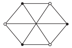
All in all, we have reached the conclusion that the effective action can be well-approximated by three coupling constants: one associated to -valent bubbles, and two associated to -valent interactions. Explicitly, we have:
| (75) |
where
| (76) | |||||
| (77) | |||||
| (78) | |||||
Each term in is represented by a drawing from the top line of Figure 8 (where colors are left implicit). In , or , there are exactly three distinct bubbles contributing, which correspond to the three possible colorings of the graphs , or respectively. Such bubbles have therefore identical coupling constants by color invariance. In addition there are four possible types of counter-terms one generates when lowering the scale from to . The first is mass, associated to the intermediate parameter and reabsorbed into . The three others are wave-function counter-terms, depending on the color on which the Laplace operator is inserted (which is graphically represented by a cross), associated to a unique parameter or equivalently .

4.3 Computation of the relevant and marginal eigendirections
Let us now investigate how the color invariant parameters , , and vary with the scale . We will also denote the eigendirections of this system , , and . In order to determine them, we first need to compute the coefficients appearing in the recursive equation:
| (79) |

The unique type of graph contributing to is represented in Figure 9. There is one such graph per color , which we label . Each such graph has a symmetry factor . One therefore finds
| (80) |
The value of , which we denote , can be straightforwardly computed:
| (81) | |||||
| (82) | |||||
| (83) |
Hence we have shown that:
| (84) |

We call the graphs contributing to , as represented in Figure 10. There are three such graphs, each of them having a symmetry factor . Remark moreover that
| (85) |
and therefore
| (86) |


Two types of graphs contribute to , they are represented in Figure 11. The value of a is again , and its symmetry factor . These graphs therefore contribute with a term to . The evaluation of a graph is
| (87) | |||||
| (88) |
In order to evaluate this limit, we resort to a Laplace approximation (see the Appendix), which turns the integral over into a Gaussian integral over a vector . This yields
| (89) |
and the Gaussian integral can be explicitly performed to give
| (90) | |||||
Since there are three graphs of the type , with trivial symmetry factors, the net contribution to is . We have thus obtained:
| (91) |

The graphs to be taken into account for the computation of are those of Figure 12. Their value is . Two graphs and with contribute to the flows of distinct -valent bubbles. The symmetry factor being , one therefore finds
| (92) |

Similarly, is determined by the graphs (see Figure 13), which have value . Two such graphs (mapped into one another by the exchange ) correspond to a single -valent effective bubble, and . This shows that
| (93) |
The eigendirections associated to the dynamical system (79) can be readily computed. One finds the following (unnormalized) vectors:
| (94) |
In the last equation, we used the approximation to get rid of the dependence of the first entry. and correspond to unstable and hence relevant directions, while and are marginal. The stability of the latter is determined by higher order contributions to the flow equations, which we analyze in the next section. The unstable directions in the plane are represented in Figure 14.
In the deep UV, the exponential suppression of the parameters of the theory along these directions imposes a non-trivial functional dependence of the parameters and from and . Indeed, assuming that the components of the vector in the directions and are small but non-vanishing at small scale , the first-order equations (74) impose that they must be respectively of order and at scales . When grows very large, we can therefore assume that vanishes in the directions and . This yields:
| (113) | |||||
| (114) |
Hence, the behaviour of the flow in this asymptotic region is determined by that of the two marginal coupling constants.

5 Second order contributions to the flow of marginal coupling constants
We now focus on second order contributions to the flows of and . For clarity of the presentation, we successively compute the coupling constants counter-terms and the wave-function renormalization. This partial results are then combined to determine the flow equations.
5.1 Coupling constants renormalization


As far as is concerned, one needs to evaluate the graphs represented in Figure 15. The contracted amplitudes of the graphs factorizes over its two face-connected components. One has already been encountered, and has value . The second factor is
| (115) | |||||
| (116) |
and can be explicitly computed:
| (117) | |||||
The symmetry factors are trivial: . At fixed , there are two graphs contributing, corresponding to the labeling of the graphs. The net contribution to is therefore:
| (118) |
Each graph also evaluates to . At fixed , there are two possible choices for the color , and the symmetry factors are again trivial. Therefore the total contribution of these graphs to is:
| (119) |
Let us now turn to the graphs . Their contracted amplitudes evaluate to:
| (120) | |||||
| (121) | |||||
| (122) | |||||
| (123) |
One can easily see that . Since at fixed there are two possible choices for which generate the same effective bubble, we conclude that these graphs produce a term
| (124) |
in the expression of .
Finally, the contracted amplitude of a graph is , and . Each of them generates a distinct effective bubble. Therefore this graphs result in a term:
| (125) |
In summary, we have just shown that:
| (126) |


We proceed in a similar way to determine . The four types of graphs contributing are represented in Figure 16.
The graphs evaluate to . At fixed , we are free to choose between two values of and the sign , therefore four distinct graphs generate the same effective bubble. Since the symmetry factors are trivial, these graphs are responsible for a term
| (127) |
in the computation of .
The amplitude of any graph is . The symmetry factors are trivial, and the value of uniquely determines the effective bubble generated by the graph. Once is fixed one has two possibilities for , and two for . Hence these graphs produce a term
| (128) |
The graphs generate a term proportional to . At fixed , there is a freedom in the choice of . Since this results in the following contribution to :
| (129) |
Finally, the graphs generate amplitudes evaluating to . At fixed , one is free to choose between two values for and two values for . The symmetry factor is , hence the total contribution of these graphs is:
| (130) |
This concludes the computation of :
| (131) |
5.2 Wave-function renormalization


The wave-function renormalization is determined, at this order, by the graphs , , and , more precisely by their Taylor expansion at order two around their local part.
Each graph generates a term:
| (134) | |||||
In order to evaluate the Gaussian integral with respect to , we re-arrange the quadratic form appearing in the exponentials:
| (135) |
so that:
| (136) |
To evaluate the integral over , we make use of the general formula:
| (137) | |||||
This finally yields:
| (138) |
The symmetry factor associated to each such graph is , therefore they collectively generate a term
| (139) |
in the expression of .
The contribution of a graph can be evaluated in a similar way. It is
| (141) | |||||
where the quadratic form is defined by:
| (142) |
One can re-arrange in such a way that one can easily integrate and successively, for instance:
| (143) | |||||
Hence:
| (144) | |||||
| (145) | |||||
| (146) |
Since , the contribution of this graphs to is:
| (147) |
Let us now consider a graph , and call , the two remaining colors. By expanding the amplitude of the graph to Taylor order around its tensor invariant part, one easily sees that a kernel of the form
| (148) |
is generated. By varying one therefore generates Laplace operators, which split equitably between the three internal colors. Therefore the total contribution of these graphs to is:
| (149) |
Finally, we can examine the contributions. Each of these amplitudes produces a term:
| (151) | |||||
where
| (152) |
One can then rewrite as
| (153) | |||||
so that
| (155) | |||||
| (156) |
Since and generate Laplacians acting on the same color, the combinatorial factor is simply . Hence these graphs generate a term:
| (157) |
in the expression of .
This concludes the computation of the wave-function parameter:
| (158) |
5.3 Resulting equations
We can now gather the results (126), (131) and (158) to deduce the flow equations for and up to second order. This yields:
(159) (160)
We notice that all the wave-function contributions come with a positive sign, as opposed to all the other terms which come with a minus sign. In order to determine how the -valent couplings behave in the UV region, one can first determine the signs of the resulting coefficients. To this purpose, we prove the following lemma:
Lemma 1.
For any :
- (i)
;
- (ii)
.
There exists , such that for any :
- (iii)
.
Proof.
To begin with, we remark that
| (161) | |||||
| (162) |
Hence
| (163) | |||||
| (164) |
This immediately yields
| (165) | |||||
| (166) | |||||
| (167) |
where in the third line we have used that .
We can prove the second inequality in a similar way:
| (168) | |||||
| (169) | |||||
| (170) |
with the last line an immediate consequence of .
In order to prove the third inequality it is sufficient to show that the derivative of with respect to converges to a strictly positive number when . One has
| (171) | |||||
| (172) |
and
| (173) | |||||
| (174) | |||||
| (175) |
This yields in particular:
| (176) |
which concludes the proof. ∎
Remark. The explicit expressions of and being rather involved, we did not try to prove that in full generality. However one can easily check numerically that this holds, as one would expect. See Figure 18.

These inequalities immediately imply that all the coefficients appearing in equations (159) and (160) are strictly positive. If one starts with small positive coupling constants at scale , and will both grow towards the infrared. One would therefore be tempted to conclude that the model is asymptotically free. However, due to the non-linear nature of the flow equations we have derived, only a careful analysis can settle this question, which is the purpose of the next and final section.
6 Qualitative behaviour in the vicinity of the Gaussian fixed point
The main purpose of this last section is to determine under which conditions the theory flows towards a Gaussian model in the deep UV. To this effect, we will analyze the qualitative properties of the continuous flow which underlies the discrete equations derived in the preceding section.
6.1 Continuous flow
The truncated system of equations we have derived in the previous sections takes the form:
Since the last three equations form a closed system, and we only wish to determine at which conditions the theory becomes Gaussian in the UV, we will ignore the mass coupling constant. We can moreover assume that the qualitative behaviour of the theory will be well-captured by a continuous version of the flow, which we now describe.
Let us introduce new effective coupling constants , and , where is to be thought of as and is a continuously varying UV cut-off1616 16 Contrary to standard notations, the UV side of the scale ladder corresponds to .. We then define the autonomous system of first-order differential equations:
| (177) |
From now on, the term ’Gaussian fixed point’ will refer to the fixed point of the system . Our goal is to determine which solutions of converge to the Gaussian fixed point in the limit .
Let us now gather a few useful facts about . First, the coefficients are all strictly positive. Second, five different planes will play a special role, as subspaces on which one of the components of the flow cancels. These are:
| (178) | ||||
| (179) | ||||
| (180) | ||||
| (181) | ||||
| (182) |
In particular, we immediately notice that on (resp. ), both (resp. ) and (resp. ). With the help of Cauchy–Lipschitz theorem, this immediately implies the following lemma:
Lemma 2.
The sign of (resp. ) is invariant under the flow of .
Thus we will conveniently organize our analysis according to the signs of and , and as a warming exercise construct the phase portrait of the flow in the invariant subspace . The following set of inequalities will prove useful in this respect.
Lemma 3.
For any :
- (i)
;
- (ii)
.
There exists , such that for any :
- (iii)
;
- (iv)
.
Proof.
One first has that:
| (183) |
which by use of formula (164) implies
| (185) |
The sign of is immediately obtained from that of :
| (186) |
The last two inequalities are again more involved, due to the complicated expressions for and . Using the explicit expression of , , and applying once more formula (164), one finds:
| (187) | |||||
| (188) |
The functions and evaluate to when , so to prove that they are positive, it is enough to show that their first derivatives are positive for any . These are given by
| (189) | |||||
| (190) |
By use of the asymptotic expansions of and , see equations (172) and (175), one obtains:
| (191) | |||||
| (192) |
In particular, one concludes that both and diverge to when , which concludes the proof. ∎
Remark. Again, even if we have not proven it in full generality, one can convince oneself that the functions and are strictly positive on (see Figure 19), which guarantees that the coefficients and are strictly positive for any value of . We also provide numerical plots of the -coefficients in Figure 20, which confirm our claims.


6.2 Phase portrait on the invariant subspace
Let us assume that and look at the reduced autonomous system:
| (193) |
According to Lemma 3, the relative positions of the lines and in the plane are as represented in Figure 21, no matter what the value of is. We define the open sets:
| (194) | ||||
| (195) | ||||
| (196) | ||||
| (197) | ||||
| (198) | ||||
| (199) |
in each of which the signs of and do not change. In Figure 21, the small arrows in each region indicate the signs of and . In particular, one notices that the only two regions in which and are both strictly increasing are and . We therefore expect that any non-trivial trajectory1717 17 That is, any trajectory not contained in the axis. converging to the Gaussian fixed point in the limit would approach it from one of these two regions. Let us now investigate in more details whether one of these scenarii actually occurs.
In the following, we denote by a maximal solution of , defined for any . Let us first focus on the case . One can first prove the following lemma.
Lemma 4.
Let . If , then one can find such that .
Proof.
Let us first assume that . If for all , then and are both decreasing with respect to . Moreover, , and hence diverges in the limit . Since for all , necessarily crosses , which yields a contradiction. Hence there must exists such that .
The non-trivial part of this lemma concerns the situation in which . If for all , then and are both monotonically increasing and bounded from below. Therefore they must converge in , and since there is no other fixed point available, converges to in the limit . Now, one also has:
| (200) |
where and we made use of Lemma 3. This implies that
| (201) |
which is incompatible with . Hence there must be a such that . ∎
This is sufficient to conclude with the following proposition.
Proposition 3.
Let . There exists no solution of such that:
| (202) |
Proof.
The flow of is outward-pointing on the boundary of . Therefore is stable with respect to the time-reversed flow of . Combined with the fact that in this region both and are increasing with respect to this time-reversed flow, the previous Lemma provides the desired result. ∎
Remark. We can easily go a bit further and show that the trajectories in the half-space are of two types: those verifying and ; and those such that . In both cases, and . See Figure 21.

Let us now consider the other half of the plane. An analogue of Lemma 4 holds in this sector.
Lemma 5.
Let . If , then there exists such that:
| (203) |
Moreover:
| (204) |
Proof.
Assume .
If for all , then and are monotonically decreasing on , and bounded from above. must therefore converge in the limit , hence to the Gaussian fixed point. This is impossible since for all , therefore there must be a such that .
Similarly, we can show that has to be in region for some . This region is stable under the flow of . Therefore is increasing, bounded on , and must therefore converge in . is decreasing, and similarly either converges or tends to in . In order to determine which of these two cases arises, notice that in the region Lemma 3 ensures that:
| (205) |
where . This yields the bound
| (206) |
for any . It therefore appears that if were to converge to a finite value in , would converge to a non-zero value, and the limit value of would not be a fixed point. Hence must tend to when .
∎
This allows to conclude that the Gaussian fixed point is UV attractive relative to negative perturbations of .
Proposition 4.
Let be a solution of and . There exists a neighborhood of such that:
| (207) |
Proof.
In order to construct an appropriate neighborhood , let us consider a solution such that and . By Lemma 5, enters in region and remains there at later times. Hence the distance between the origin and the curve is non-zero. Reparameterizing the trajectory of by the function , we define the open set:
| (208) | ||||
which contains the origin. In the half-plane , coincides with the greyed region in Figure 21.
It is easy to check that is stable with respect to the time-reversed flow of . Indeed, this flow evaluated on the boundary of is either tangential (on ) or inward-pointing (on ).
Consider now a solution such that and . If , one can find such that . If not, and being monotonic on and bounded, they would have to converge in , hence to . But this cannot be since one would also have for any . This observation, together with Lemma 5 implies the existence of some such that , and hence for all . On , is increasing and bounded from below by , therefore converges in . Similarly, converges in . Since the only fixed point available is the Gaussian one, converges to when . ∎
Remark. Like in the previous case, one could try to map the flow more precisely in this region. However this would require more involved computations. Since from a physical perspective we are only interested in the properties of the flow of in the vicinity of the trivial fixed point, we decided to ignore possible complications arising from trajectories reaching simultaneously large negative values of and . That was the technical purpose of the introduction of the open set . See Figure 21.
Similar results can be proven with the same methods in the plane: no trajectory with is asymptotically free, and on the contrary all trajectories with are.
6.3 General properties of trajectories with
We now come back to the full three-dimensional system . It turns out that the case in which and have identical signs can be analyzed in a way very similar to what has been achieved in the previous section. We can first infer the relative positions of the planes , and from Lemma 3 (and our numerical checks).
Lemma 6.
If and , then:
| (209) |
If and , then:
| (210) |
This allows us to define the disjoint open sets
| (211) | ||||
| (212) | ||||
| (213) | ||||
| (214) | ||||
| (215) |
which moreover verify
| (216) | |||
| (217) |
In the following denotes a maximal solution of . We can first show that in the subspace, all trajectories must intersect at early times.
Lemma 7.
Let . If , then one can find such that .
Proof.
Let us first assume that . Since , and are all negative in this region, we can repeat the argument of Lemma 4 and conclude that cannot remain within at all times , and hence must enter region .
It hence appears that there are no asymptotically free trajectories with both and .
Proposition 5.
Let . There exists no solution of such that:
| (219) |
Proof.
One only needs to check that the region , in which , is stable with respect to the time-reversed flow of . This is guaranteed by the following facts:
| (220) |
on ;
| (221) |
on ; and
| (222) |
on . ∎
The previous proposition is the main result of this paper: the hypothesis that the Gaussian fixed point is UV stable against perturbations and , as suggested by equations (159) and (160), is not confirmed by a careful inspection of the equations.
We now consider the situation in which both and are negative. As compared to the previous section, we will avoid unnecessary complications by relying even more on a suitably chosen stable neighborhood of the origin.
Lemma 8.
Suppose that for some . Then:
| (223) |
Proof.
We can first remark that is stable with respect to the flow of . Indeed one has
| (224) |
for any such that and . Hence is monotonically decreasing on , and one of the two following cases occur: a) , or b) .
Assuming that a) is realized, then also . It results that must asymptotically reach the set . But unless , in which case . This implies that must converge to the Gaussian fixed point in .
Let us now show that this behaviour is not consistent with the flow equations. When and , Lemma 3 allows to prove that:
| (225) |
where and . These in turn imply
| (226) |
for any . These two inequalities are incompatible with .
Hence the situation b) is the one which actually occurs. ∎
Proposition 6.
Let be a solution of and . There exists a neighborhood of such that:
| (227) |
Proof.
Let us define the open disc
| (228) |
The flow of generates the set
| (229) |
which according to Lemma 8 is infinitely extended in the direction . See Figure 22 for a qualitative representation of and . Then
| (230) |
is an open set containing the origin. Moreover, is by construction stable under the time-reversed flow of .
Assume that . If for all , then is a monotonically decreasing function. Moreover, since is bounded on , must converge in . Then one also has when , therefore by the same argument as already invoked in Lemma 8 one must have . If on the other hand for some , then for any . By monotonicity and boundedness of , and , one then again concludes that .
Finally, the case in which has already been treated in the previous section, and similar results hold for . ∎

6.4 Trajectories with
The phase portrait in regions in which and have opposite signs is more difficult to analyze.
On the one hand, there is no obvious UV stable open set in which , and are simultaneously strictly increasing under the flow of . Hence there seems to be no immediately identifiable argument proving that asymptotically free trajectories do exist in this region. On the other hand, none of the bounds we relied on in the previous sections (in particular to exclude asymptotic freedom when and ), are easily generalizable. Therefore the non-existence of asymptotically free trajectories in this sector seems equally hard to establish.
In a sense the dynamical system becomes truly three dimensional when , with all the complications this may lead to. A comprehensive study in this regime is therefore beyond the scope of the present work, and we leave the question open for future investigations.
7 Conclusion and outlook
Let us start with a summary of what has been achieved in this paper. The main goal was to develop a Wilsonian renormalization group picture of the renormalizable TGFT of [52]. This required the introduction of dimensionless parameters, with canonical dimensions inferred from the power-counting. The perturbative expansion was then performed with respect to the dimensionless parameters rather than the dimensionful ones, which is responsible for subtle departures with respect to previous analyzes of such models [55, 56, 52]: the class of graphs which are divergent in this sense is enlarged. General (and formal) flow equations, involving melonic graphs only, have been derived.
We then applied these general equations in the vicinity of the Gaussian fixed point, where perturbation theory can be applied. We first recovered the splitting between renormalizable and non-renormalizable coupling constants, which allowed us to restrict ourselves to four independent parameters: the mass, a -valent coupling constant, and two -valent coupling constants. The eigendirections of the linearized system were then computed, reducing further the set of independent couplings in the deep UV region: the mass and -valent coupling constant become linearly dependent of the two marginal -valent coupling constants at high scales. In order to fully understand the flow in the vicinity of the Gaussian fixed point, the perturbative expansion was pushed to second order in the marginal parameters. Resorting to continuous methods, we eventually derived some general properties. Our main result is the following (see Proposition 5):
Renormalization group trajectories with non-zero and positive marginal parameters are not asymptotically free.
For such trajectories, the existence of a Landau pole can therefore not be excluded. On the contrary, we also proved that the Gaussian fixed point is UV attractive with respect to negative perturbations of the marginal parameters (see Proposition 6). However this corresponds to a regime in which one does not expect to be able to define the partition function rigorously.
A few comments are in order as far as asymptotic freedom is concerned. As was made clear in previous works [55, 56], asymptotic freedom is to be expected in such models, due to an enhanced wave-function renormalization as compared to ordinary scalar field theories. Indeed, tadpoles are not exactly local (i.e. tensorial) in TGFTs, and therefore wave-function counter-terms appear already at first order in the perturbative expansion. If big enough, these terms can balance the first-order coupling constant counter-terms and make the -function negative. This is exactly what happens in [55, 56], and also what seems to happen in the present paper, see equations (159) and (160). However, our analysis shows that the non-linear terms appearing in equations (159) and (160) spoil these expectations. The non-trivial dynamics of the -valent coupling constant and the two marginal coupling constants and yield a complicated phase portrait (already in the vicinity of the origin), as is well illustrated by Figure 21.
Note also that our construction relies heavily on the introduction of dimensionless parameters. While this is required and well-understood in ordinary quantum field theory, the same procedure in TGFT deserves more clarification. It is indeed based on a more abstract notion of dimensionality given by the power-counting, and not immediately interpretable in terms of physical dimensions such as lengths, energies etc. It depends in particular on the choice of propagator, of Laplace-type in our situation, which is one other aspect of TGFTs for which a clear physical interpretation is lacking. Note also that in renormalizable models with quartic interactions, a computation along the lines of [55, 56] and the discrete renormalization group picture developed in this paper would match. Therefore we expect such models to be asymptotically free. Good candidates in TGFTs with gauge invariance condition are rank- models on dimension groups [60], rank- models on dimension groups, and rank- models on dimension groups (see the full classification of renormalizable models in [52, 54]).
Finally, while our analysis excludes the existence of asymptotically free trajectories in this model when and , it does not prove the existence of a Landau pole either. Moreover, we did not include a detailed investigation of the situation in which and have opposite signs, which as we have argued is probably involved, but might simultaneously support asymptotic freedom and convergence of the path-integral. Therefore the question of the existence of this model with no cut-off remains open, and could be investigated further. In particular, our calculations are consistent with the existence of a non-trivial UV fixed point with , , and . More generally, the existence of non-trivial fixed points for this model will be first investigated by means of an -expansion [60]. Similarly to ordinary scalar field theories, one can indeed construct renormalizable TGFT models on groups of dimension (see [52] and [54]), and then analytically continue the dimension to . This procedure should give first hints about the model. It will then be desirable to investigate the same questions with different and more adapted tools, such as the Functional Renormalization Group [59, 36].
Acknowledgments
I would like to thank Dine Ousmane Samary and Joseph Ben Geloun for discussions, especially in the early stages of this work. I am also grateful to Daniele Oriti and Vincent Rivasseau for their comments on a draft version of this paper. The final version greatly benefited from insightful remarks I owe to Razvan Gurau and an anonymous referee, which I wish to acknowledge.
Appendix: Laplace approximation
Two properties are involved in the evaluation of the amplitudes at large scales. The first one is the short time asymptotics of the heat-kernel
| (231) |
valid on any compact which does not contain . is the class angle of , defined by
| (232) |
and is the norm of . We can use the orthonormal basis , with the Pauli matrices. We then have:
| (233) |
In what follows, we shall adopt a vectorial notation for scalar products between Lie algebra elements.
The second property we use in the computations is that arbitrarily close to the identity, the normalized Haar measure is equivalent to the Lebesgue measure on the Lie algebra :
| (234) |
Consider now an integral of the form
| (235) |
where: and are finite sets such that, for any , ; or ; and for any . Let us moreover assume that:
| (236) |
When the parameters are simultaneously sent to , the integrand of is more and more peaked around the configurations such that
| (237) |
for any . By hypothesis, the unique such configuration is . One can therefore linearize the variables around the identity to accurately estimate the integral. Using this idea in combination with (231) and (234) one finds that:
| (238) | |||||
Hence determining the asymptotic behaviour of reduces to the computation of a Gaussian integral. Such formula have already been used in the literature, for instance in [57] and [61].
References
- [1] Laurent Freidel. Group field theory: An Overview. Int.J.Theor.Phys., 44:1769–1783, 2005, hep-th/0505016.
- [2] Daniele Oriti. The Group field theory approach to quantum gravity. 2006, gr-qc/0607032.
- [3] Daniele Oriti. The microscopic dynamics of quantum space as a group field theory. pages 257–320, 2011, 1110.5606.
- [4] Thomas Krajewski. Group field theories. PoS, QGQGS2011:005, 2011, 1210.6257.
- [5] Jan Ambjorn, Bergfinnur Durhuus, and Thordur Jonsson. Three-dimensional simplicial quantum gravity and generalized matrix models. Mod.Phys.Lett., A6:1133–1146, 1991.
- [6] Mark Gross. Tensor models and simplicial quantum gravity in 2-D. Nucl.Phys.Proc.Suppl., 25A:144–149, 1992.
- [7] Naoki Sasakura. Tensor model for gravity and orientability of manifold. Mod.Phys.Lett., A6:2613–2624, 1991.
- [8] Razvan Gurau and James P. Ryan. Colored Tensor Models - a review. SIGMA, 8:020, 2012, 1109.4812.
- [9] Vincent Rivasseau. The Tensor Track: an Update. 2012, 1209.5284.
- [10] Abhay Ashtekar and Ranjeet S Tate. Lectures on non-perturbative canonical gravity, volume 6. World Scientific Publishing Company Incorporated, 1991.
- [11] Carlo Rovelli. Quantum gravity. Cambridge University Press, 2004.
- [12] Thomas Thiemann. Modern canonical quantum general relativity. Cambridge University Press, 2007.
- [13] Rodolfo Gambini and Jorge Pullin. A first course in Loop Quantum Gravity. Oxford University Press, USA, 2011.
- [14] Martin Bojowald. Canonical gravity and applications. Cambridge University Press Cambridge, 2011.
- [15] Alejandro Perez. The Spin Foam Approach to Quantum Gravity. Living Rev.Rel., 16:3, 2013, 1205.2019.
- [16] John C. Baez. Spin foam models. Class.Quant.Grav., 15:1827–1858, 1998, gr-qc/9709052.
- [17] Daniele Oriti. Spacetime geometry from algebra: spin foam models for non-perturbative quantum gravity. Reports on Progress in Physics, 64(12):1703, 2001.
- [18] Sergei Alexandrov, Marc Geiller, and Karim Noui. Spin Foams and Canonical Quantization. SIGMA, 8:055, 2012, 1112.1961.
- [19] Daniele Oriti. Group field theory as the microscopic description of the quantum spacetime fluid: A New perspective on the continuum in quantum gravity. PoS, QG-PH:030, 2007, 0710.3276.
- [20] Roberto De Pietri, Laurent Freidel, Kirill Krasnov, and Carlo Rovelli. Barrett-Crane model from a Boulatov-Ooguri field theory over a homogeneous space. Nucl.Phys., B574:785–806, 2000, hep-th/9907154.
- [21] Michael P. Reisenberger and Carlo Rovelli. Space-time as a Feynman diagram: The Connection formulation. Class.Quant.Grav., 18:121–140, 2001, gr-qc/0002095.
- [22] Bianca Dittrich. From the discrete to the continuous: Towards a cylindrically consistent dynamics. New J.Phys., 14:123004, 2012, 1205.6127.
- [23] Bianca Dittrich. How to construct diffeomorphism symmetry on the lattice. PoS, QGQGS2011:012, 2011, 1201.3840.
- [24] Benjamin Bahr, Bianca Dittrich, Frank Hellmann, and Wojciech Kaminski. Holonomy Spin Foam Models: Definition and Coarse Graining. Phys.Rev., D87:044048, 2013, 1208.3388.
- [25] Daniele Oriti. Group field theory as the 2nd quantization of Loop Quantum Gravity. 2013, 1310.7786.
- [26] Steffen Gielen, Daniele Oriti, and Lorenzo Sindoni. Cosmology from Group Field Theory Formalism for Quantum Gravity. Phys.Rev.Lett., 111(3):031301, 2013, 1303.3576.
- [27] Steffen Gielen, Daniele Oriti, and Lorenzo Sindoni. Homogeneous cosmologies as group field theory condensates. JHEP, 1406:013, 2014, 1311.1238.
- [28] Razvan Gurau. Colored Group Field Theory. Commun.Math.Phys., 304:69–93, 2011, 0907.2582.
- [29] Razvan Gurau. The 1/N expansion of colored tensor models. Annales Henri Poincare, 12:829–847, 2011, 1011.2726.
- [30] Razvan Gurau and Vincent Rivasseau. The 1/N expansion of colored tensor models in arbitrary dimension. Europhys.Lett., 95:50004, 2011, 1101.4182.
- [31] Razvan Gurau. The complete 1/N expansion of colored tensor models in arbitrary dimension. Annales Henri Poincare, 13:399–423, 2012, 1102.5759.
- [32] Razvan Gurau. A generalization of the Virasoro algebra to arbitrary dimensions. Nucl.Phys., B852:592–614, 2011, 1105.6072.
- [33] Razvan Gurau. Universality for Random Tensors. 2011, 1111.0519.
- [34] Valentin Bonzom, Razvan Gurau, and Vincent Rivasseau. Random tensor models in the large N limit: Uncoloring the colored tensor models. Phys.Rev., D85:084037, 2012, 1202.3637.
- [35] Vincent Rivasseau. The Tensor Track, III. 2013, 1311.1461.
- [36] Vincent Rivasseau. The Tensor Theory Space. 2014, 1407.0284.
- [37] Valentin Bonzom, Razvan Gurau, Aldo Riello, and Vincent Rivasseau. Critical behavior of colored tensor models in the large N limit. Nucl.Phys., B853:174–195, 2011, 1105.3122.
- [38] Dario Benedetti and Razvan Gurau. Phase Transition in Dually Weighted Colored Tensor Models. Nucl.Phys., B855:420–437, 2012, 1108.5389.
- [39] Valentin Bonzom. Revisiting random tensor models at large N via the Schwinger-Dyson equations. JHEP, 1303:160, 2013, 1208.6216.
- [40] Valentin Bonzom. New 1/N expansions in random tensor models. JHEP, 1306:062, 2013, 1211.1657.
- [41] Razvan Gurau and James P. Ryan. Melons are branched polymers. 2013, 1302.4386.
- [42] Wojciech Kaminski, Daniele Oriti, and James P. Ryan. Towards a double-scaling limit for tensor models: probing sub-dominant orders. 2013, 1304.6934.
- [43] Stéphane Dartois, Razvan Gurau, and Vincent Rivasseau. Double Scaling in Tensor Models with a Quartic Interaction. JHEP, 1309:088, 2013, 1307.5281.
- [44] Valentin Bonzom, Razvan Gurau, James P. Ryan, and Adrian Tanasa. The double scaling limit of random tensor models. 2014, 1404.7517.
- [45] Razvan Gurau. The 1/N Expansion of Tensor Models Beyond Perturbation Theory. Commun.Math.Phys., 330:973–1019, 2014, 1304.2666.
- [46] Thibault Delepouve, Razvan Gurau, and Vincent Rivasseau. Borel summability and the non perturbative expansion of arbitrary quartic tensor models. 2014, 1403.0170.
- [47] Joseph Ben Geloun and Vincent Rivasseau. A Renormalizable 4-Dimensional Tensor Field Theory. Commun.Math.Phys., 318:69–109, 2013, 1111.4997.
- [48] Joseph Ben Geloun and Dine Ousmane Samary. 3D Tensor Field Theory: Renormalization and One-loop -functions. Annales Henri Poincare, 14:1599–1642, 2013, 1201.0176.
- [49] Joseph Ben Geloun. Renormalizable Models in Rank Tensorial Group Field Theory. 2013, 1306.1201.
- [50] Joseph Ben Geloun and Etera R. Livine. Some classes of renormalizable tensor models. J.Math.Phys., 54:082303, 2013, 1207.0416.
- [51] Sylvain Carrozza, Daniele Oriti, and Vincent Rivasseau. Renormalization of Tensorial Group Field Theories: Abelian U(1) Models in Four Dimensions. Commun.Math.Phys., 327:603–641, 2014, 1207.6734.
- [52] Sylvain Carrozza, Daniele Oriti, and Vincent Rivasseau. Renormalization of a SU(2) Tensorial Group Field Theory in Three Dimensions. Commun.Math.Phys., 330:581–637, 2014, 1303.6772.
- [53] Dine Ousmane Samary and Fabien Vignes-Tourneret. Just Renormalizable TGFT’s on with Gauge Invariance. Commun.Math.Phys., 329:545–578, 2014, 1211.2618.
- [54] Sylvain Carrozza. Tensorial Methods and Renormalization in Group Field Theories. Springer Theses, 2014.
- [55] Joseph Ben Geloun. Two and four-loop -functions of rank 4 renormalizable tensor field theories. Class.Quant.Grav., 29:235011, 2012, 1205.5513.
- [56] Dine Ousmane Samary. Beta functions of gauge invariant just renormalizable tensor models. Phys.Rev., D88(10):105003, 2013, 1303.7256.
- [57] Joseph Ben Geloun and Valentin Bonzom. Radiative corrections in the Boulatov-Ooguri tensor model: The 2-point function. Int.J.Theor.Phys., 50:2819–2841, 2011, 1101.4294.
- [58] Joseph Ben Geloun, Thomas Krajewski, Jacques Magnen, and Vincent Rivasseau. Linearized Group Field Theory and Power Counting Theorems. Class.Quant.Grav., 27:155012, 2010, 1002.3592.
- [59] Astrid Eichhorn and Tim Koslowski. Continuum limit in matrix models for quantum gravity from the Functional Renormalization Group. Phys.Rev., D88:084016, 2013, 1309.1690.
- [60] Sylvain Carrozza. Group Field Theory in Dimension . To appear.
- [61] Aristide Baratin, Sylvain Carrozza, Daniele Oriti, James Ryan, and Matteo Smerlak. Melonic phase transition in group field theory. Lett.Math.Phys., 104:1003–1017, 2014, 1307.5026.