IPhT T14/100
CRM-3339
Root systems, spectral curves, and analysis of a Chern-Simons matrix model for Seifert fibered spaces
Gaëtan Borot11 1 Section de Mathématiques, Université de Genève, 2-4 rue du Lièvre 1206 Genève, Switzerland.22 2 MIT, Maths Department, Massachusetts Avenue 77, Cambridge 02139, USA33 3 Max Planck Institut für Mathematik, Vivatsgasse 7, 53111 Bonn, Germany., Bertrand Eynard 44 4 Institut de Physique Théorique, CEA Saclay, Orme des Merisiers, 91191 Gif-sur-Yvette, France.55 5 Centre de Recherches Mathématiques, 2920, Chemin de la Tour, Montréal, QC, Canada.
with a section by Alexander Weisse3
Abstract
We study a class of scalar, linear, non-local Riemann-Hilbert problems (RHP) involving finite subgroups of . We associate to such problems a (maybe infinite) root system and describe the relevance of the orbits of the Weyl group in the construction of its solutions. As an application, we study in detail the large expansion of and Chern-Simons partition function of -manifolds that are either rational homology spheres or more generally Seifert fibered spaces. It has a matrix model-like representation, whose spectral curve can be characterized in terms of a RHP as above. When is finite (i.e. for manifolds that are quotients of by a finite isometry group of type ADE), the Weyl group associated to the RHP is finite and the spectral curve is algebraic and can be in principle computed. We then show that the large expansion of is computed by the topological recursion. This has consequences for the analyticity properties of perturbative invariants of knots along fibers in .
*
Acknowledgements
G.B. thanks Andrea Brini, Réda Chhaibi, Thomas Haettel, Neil Hoffman, Thang Lê, Alexei Oblomkov, George Thompson, and especially Albrecht Klemm, Stavros Garoufalidis and Marcos Mariño for comments and fruitful discussions, as well as the organizers of the Quantum Topology and Hyperbolic Geometry conference in Nha Trang (May 2013), where a preliminary version of this work was presented. Marcos Mariño and Alba Grassi collaborated in an earlier phase to the Section 8 concerning Kauffman invariants. This work benefited from the support of Fonds Européen S16905 (UE7–CONFRA), the Swiss NSF, the Max-Planck-Gesellschaft, and the Simons foundation.
B.E. thanks T. Kimura, the CRM Montréal, the FQRNT grant from the Québec government, P. Sułkowski and the ERC starting grant Fields-Knots, S. Smirnov and the University of Geneva.
AMS Classification: 14Hxx, 45Exx, 51Pxx, 57M27, 60B20, 81T45.
1 Introduction
Unless mentioned otherwise, the orbit space of Seifert fibered spaces in this article is assumed to be a sphere.
1.1 Scope
denotes a semi-simple Lie algebra, and its Cartan subalgebra, identified with . We shall study the probability measure over :
| (1.1) |
where the product ranges over positive roots of , is a positive parameter, and the partition function is such that . We are interested in the series of Lie algebras, in the regime where the rank goes to .
The model (1.1) arises in Chern-Simons theory with gauge group on a simple class of -manifolds called Seifert fibered spaces [38]: roughly speaking, these are -fibrations over a surface orbifold, here assumed to be topologically a sphere. (1.1) captures the contribution of the trivial flat connection in perturbative Chern-Simons theory, or equivalent, the evaluation of the LMO invariants of in the weight system defined by [37, 1, 2, 2, 3]. Moreover, the correlation functions in (1.1) compute the colored HOMFLY (in any representation of fixed size) of the knots going along the fibers of , see § 4.4. The regime has aroused interest since it allows a rigorous definition of perturbative invariants ensuing from and the colored HOMFLY of links in , which should be related via geometric transitions to topological strings invariants in according to the physics literature [47], see § 1.4.
General arguments [14] show that the large asymptotic expansion of models of the type (1.1) – once it is proven to exist using the tools of [15] – can be computed by the topological recursion of [22]. It then remains to compute the initial data of the recursion : is related to the equilibrium measure of (2.1), also called spectral curve, and is related to the large limit of the -point correlation function. Both are characterized by a saddle point equation which takes the form of a linear but non-local Riemann-Hilbert problem (RHP) on a cut locus to determine. Addressing its solution is an important part of our present work. We shall devise in Section 3 a general method to construct the solution of a large class of RHP where the jumps are obtained by action of a finite subgroup of Möbius transformations. We actually build the – maybe infinite – monodromy group of the solution, and relate it to the Weyl group of a root system. The solution can be studied in more details by algebro-geometric means when this Weyl group is finite. This construction applies to the computation of relevant for (2.1), but has also its own interest and can be used as a tool in other problems.
Our work has two noteworthy consequences for knot theory.
Firstly, we obtain analyticity results on perturbative invariants of knots in manifolds different from the -sphere. The colored HOMFLY of links in are polynomials (after a suitable normalization) in and . This is clear from skein theory, and can also be explained from quantum field theory perspective [48]. This implies that the coefficients in the expansion while keeping fixed, produce polynomials in . These properties are not expected to be true for invariants of links in other -manifolds. We show how to compute invariants of fiber knots in Seifert fibered spaces. Remarkably, the position of the singularities in the -complex plane only depend on the ambient -manifold. They occur at the singularities of the family of spectral curves (parametrized by ) associated to (1.1). We conjecture more generally that for any link in a rational homology sphere , the singularities of the perturbative invariants only depend on the ambient manifold . More precise statements of the conjecture described in § 4.2.2.
Secondly, we find that the spectral curves and the perturbative invariants for the colored Kauffman perturbative invariants (associated to the Lie algebra) are closely related to the more conventional invariants ( series), and we show they can all be computed by the topological recursion. The only difference is that the topological grading is not respected for the cases. We think this has an interest, since very few was known so far on perturbative Kauffman invariants.
1.2 Outline and main results: matrix model
We establish in Section 2 the large behavior and asymptotic expansion of the partition function and moments of (1.1) for (Section 2). Some of the technical proofs are postponed to Appendix A. Section 3 is independent of the main body of the text: we introduce in (3.1) a class of linear non-local RHP, to which we associate a (maybe infinite) root system. Many information on the solution – and sometimes its full and explicit form – can be extracted from the analysis of this root system.
We review the geometry of Seifert spaces and Chern-Simons theory at large in Section 4. An important geometric invariant of Seifert spaces is the orbifold Euler characteristic of their orbit space, here always assumed to be topologically a sphere :
| (1.2) |
where are integers prescribing the orders of extraordinary fibers. We also introduce:
| (1.3) |
Section 5-7 are devoted to the Chern-Simons matrix model for Seifert fibered spaces, and their extension to the or Lie algebra is the matter of Section 8. Chern-Simons theory around the trivial flat connection depends on the single parameter:
| (1.4) |
where is another geometric parameter of the Seifert spaces. is sometimes called the string coupling constant. In Section 5, we apply the techniques of Section 3 to the construction of the spectral curves for Seifert spaces. We find in Theorem 6.1 that the finite quotients corresponding to can be described in terms of an algebraic spectral curve , whereas the spectral curve – if it exists – is never algebraic when . We will not insist on the cases , which are resonant.
Proposition 1.1
The Chern-Simons matrix model for Seifert fibered spaces with admits a spectral curve of the form for a -dependent polynomial whose Newton polygon is known. The coefficients on the boundary of the Newton polygon are known monomials in . Besides, the spectral curve comes with the action of a finite Weyl group on the sheets of , as tabulated below.
This table assumes for the lens spaces.
We were able in Section 6:
-
to determine the curves in the cases (resp. ) up to (resp. ) parameters fixed by complicated algebraic constraints.
Our spectral curve computations are supported by Monte-Carlo simulations of Alexander Weisse presented in Section 9. Bases on numerics, we also give conjectures about the spectral curve in the cases (Conjecture 2.5).
Although the genus of the spectral curve can be quite large, it does not prevent them to cover in a simple way curves of a lower genus. The completely solved cases mentioned above and our computations leads us to:
Conjecture 1.2
Assume . In the spectral curves describing the contribution of the trivial flat connection to the Chern-Simons partition function, if one eliminates from the equations and , we obtain an equation describing a (in general : singular and with several components) curve of genus .
1.3 Outline and main results: knot theory
In Section 7, we explain a practical consequence for knot theory: we can provide some informations on the analyticity properties of the coefficients (seen as functions of ) of the large expansion of the colored HOMFLY polynomials of fiber knots in , and of the Chern-Simons free energy. So far, they were only known to be analytic in a vicinity of [26]. We prove in Section 7:
Proposition 1.3
The perturbative colored HOMFLY invariants of fiber knots in a Seifert fibered space with geometry for even, defined initially as elements of , are actually the Taylor expansion of an element , where:
| (1.5) |
corresponds to , and introduced in (4.3) is a geometric parameter of the Seifert spaces. The singularities in the -complex plane occur when where:
| (1.6) |
A result similar to Proposition 1.3, with replaced by , can be deduced from Section 7-8 for the perturbative colored Kauffman invariant of fiber knots in with even.
The situation is different from links in lens spaces, where the perturbative invariants are polynomials in [17], and thus had no singularities in the -complex plane. Our work suggests the general conjectures:
Conjecture 1.4
If is a Seifert fibered space, the and the perturbative invariants of any link in exist as a function of , and are real-analytic on the positive real line.
Conjecture 1.5
Moreover, if , there exists a finite degree extension of depending only on the ambient manifold and the series of Lie algebra, such that, at least for fiber knots, the perturbative invariants colored in any representation are the Laurent expansion at of elements of .
1.4 Motivation from topological strings
The present work generalizes the analysis of the model [29, 17] relevant to study lens spaces, and the invariant of fiber knots in lens spaces are equal to invariants of torus knots in . Chern-Simons theory on at large is dual to type A open topological strings on [47], and through geometric transitions, this can sometimes be related to closed topological strings on another target space . This program has been completed for [28] and the lens spaces [29, 17] and is obtained by fractional framing transformations from the resolved conifold in both cases. So far, it has remained elusive for general Seifert fibered spaces. Since we establish the existence of an algebraic spectral curve for all Seifert spaces with , this gives hope for the construction of their mirror geometries . This direction, and the connection with gauge theories and quantum spectral curves, is under investigation [12].
A natural strategy to establish a duality to a closed string geometry would then be to prove that Gromov-Witten invariants of are also computed by the topological recursion, with same curve . So far, the topological recursion is indeed known to compute Gromov-Witten invariants when is a toric -fold Calabi-Yau [16, 23], but this might be generalized in the future to a more general class of manifolds.
2 The matrix model
2.1 Equilibrium measures
We study the statistical mechanics of particles, of position , with joint probability distribution:
| (2.1) |
At this stage, are arbitrary positive parameters. The dominant contribution to the partition function when should come from configurations maximizing the probability density. It is reasonable to think that the empirical distribution:
| (2.2) |
of such configurations will be close to a minimizer of the energy functional:
| (2.3) |
among probability measures . is actually defined in because of the singularity of the logarithm. It is a lower semi-continuous functional, so has compact level sets for the weak-* topology, therefore it achieves its minimum. We call equilibrium measure and denote any minimizer of . It must satisfy the saddle point equation: there exist a constant such that
| (2.4) |
with equality -everywhere. is the effective potential felt by a particle at position , taking into account the collective effect of all other ’s distributed according to . Equilibrium measures are characterized by the property that the effective potential achieves its minimum on the locus of where the particles accumulate. Classical techniques66 6 The arguments of [43] were developed for the pairwise interaction which has a zero at coinciding points, but it is easy to generalize to any interaction which has the same singularity and is smooth elsewhere. of potential theory [43] show that the random measure ’s limit points are equilibrium measures, and that:
| (2.5) |
Some qualitative properties of the equilibrium measures can be derived from their characterization: grows sufficiently fast at infinity to ensure that equilibrium measures have compact support ; since and the pairwise interactions are analytic (away from the singularity at ), it can be shown (see [15], generalizing [18] where was considered) that equilibrium measures are supported on a finite number of segments, have a density which is analytic away from the edges, and is -Hölder at the edges. When the density vanishes exactly like a squareroot at the edges, it is said off-critical.
The question of uniqueness of has no easy answer. But, since the functional is quadratic, if the quadratic form over the space of differences of probability measures:
| (2.6) |
is positive definite, then is strictly concave and this guarantees uniqueness of its minimizer. Notice again that, a priori, takes values in . Indeed, the singular part of is:
| (2.7) |
and the right-hand side can be infinite if the measure is not regular enough. Here is the Fourier transform of the finite mesure . As a matter of fact, it is enough to consider and as functionals over measures with compact support, because grows fast at infinity compared to the pairwise interactions.
Lemma 2.1
For any :
| (2.8) |
is definite positive whenever the function is almost everywhere positive. In particular, it must be positive at , which gives the necessary condition:
| (2.9) |
In the model for Seifert fibered spaces, the are assigned integer values. We recognize in (2.9) the orbifold Euler characteristics of the orbit space, and the list of uples leading to is finite. For and , is obviously positive definite, and for the remaining cases having , positivity can be checked by a direct computation.
Corollary 2.2
If are integers, is definite positive iff . In those cases, there exists a unique equilibrium measure.
The proof of Lemma 2.1 and Corollary 2.2 are presented in Appendix A.1 and A.2. We can also establish – see Appendix A.3 – some qualitative properties of equilibrium measures:
Theorem 2.3
For any , and any , any equilibrium measure is supported on a single segment, and vanishes exactly as a squareroot at the edges (generic edge).
Corollary 2.4
If , since the equilibrium measure is unique, it must be invariant under . In particular, its support is a segment centered at the origin.
In Section 9, Weisse proposes a Monte-Carlo simulation to obtain the dominant configurations of probability densities like (2.1). It is observed that, for any value of integers and , independently of the sign of , the empirical measure seem to have a unique limit point. It supports the
Conjecture 2.5
For any and , the equilibrium measure is unique, and its density away from the edges of the support is a real-analytic function of .
2.2 Change of variable and saddle point equation
We introduce the exponential variables:
| (2.10) |
The measure (2.1) on transforms into a measure on :
| (2.11) |
where:
| (2.12) |
and denotes a primitive -root of unity.
denote an equilibrium measure for . It is the image via (2.10) of an equilibrium measure for . It is characterized by the saddle point equation:
| (2.13) |
for some constant , with equality on the support of . We shall rewrite the characterization of an equilibrium measure in term of its Stieltjes transform:
| (2.14) |
is a bounded, holomorphic function on , such that:
| (2.15) |
The saddle point equation (2.13) implies a functional equation:
| (2.16) |
with:
| (2.17) |
The contour of integration in (2.16) can be moved to pick up residues at rotations of of order :
| (2.18) |
Since is invariant under , in the case where the equilibrium measure is unique, it must have the same symmetry. This translates into the palindrome symmetry:
| (2.19) |
When is definite positive and is fixed, (2.18) characterizes among the holomorphic functions in satisfying (2.15) and whose discontinuity on defines an integrable measure (see e.g. the argument of [14, Lemma 3.10]). When is not definite positive, we do not know how to address the question of uniqueness.
2.3 Asymptotic analysis
We rely on the results of [15] to study the asymptotic expansion when of the model (2.11). We would like to compute the partition function and the -point correlators:
| (2.20) |
where stands for ”connected expectation value”.
Definition 2.6
We say that is off-critical if its density is nowhere vanishing on its support , and it vanishes exactly like a squareroot at the edges of .
Theorem 2.7
[15] Assume is strictly concave and is off-critical. Then, we have an asymptotic expansion of the form:
| (2.21) |
The coefficients of expansion are real analytic functions of , and are holomorphic functions in .
2.4 Two point function
Definition 2.8
We call -point function:
| (2.23) | |||||
It can be obtained formally from by an infinitesimal variation of the potential :
| (2.24) |
It also satisfies also a saddle point equation, which can be obtained by formally applying the variation of the potential to the saddle point equation (2.18) satisfied by . The result is that is holomorphic in , and has a discontinuity when and satisfying:
| (2.25) | |||||
The data of is called the spectral curve. Together with the two-point function , it provides the initial data for the the recursive computation of and . We give in Section 3 general principles to solve the homogeneous linear equation, that will be put in practice to compute these data in the Seifert models (Section 4-5).
3 Algebraic theory of sheet transitions
3.1 The problem
The form taken by the saddle point equation (2.16) motivates a general study of homogeneous functional relations of the type:
| (3.1) |
where:
-
is a finite subgroup of , acting on the Riemann sphere by Möbius transformations (their classification is reminded in Appendix B).
-
is a generating subset of , not containing , and stable by inverse. is a sequence of numbers in a number field (for instance ), and we assume:
(3.2) -
is a collection of arcs on the Riemann sphere such that whenever . denotes the set of interior points of .
-
is an open subset of containing and stable under the action of , and is a holomorphic function on , that admits boundary values at any interior point of . For simplicity, will be or here.
This problem is usually supplemented with some growth prescription for at the edges of and at the boundary of . For instance, if , one can ask for prescribed singular behavior at and . This problem can also be studied with few modifications for a section of a vector bundle over , in particular for a holomorphic 1-form.
This problem for 1-form77 7 For Seifert spaces, consists of linear maps (rotations), and the extra factor of put in the definition of the Stieltjes transform (2.14) is the trick allowing the formulation of the linear equation with constant coefficients ’s in terms of a function instead of a -form. actually appears in the study of equilibrium measures for models of the form (2.11) with arbitrary (analytic) pairwise interaction . The dependence in the potential only affects the right-hand side of such an equation, which can be set to by subtracting a particular solution, thus affecting the growth prescriptions for the solution we are looking for. In general, is the Galois group of the equation , and may be complicated even for simple . It may not be finite, and the description of the orbit of has to deal with the rich question of iterating functions in the complex plane. Here, we restrict to a subclass of model where the iteration problem is trivial, in the sense that is a finite group of (globally defined) automorphisms of the Riemann sphere. The assumption that is stable under inversion comes from the fact that pairwise interactions are symmetric . One can go beyond this assumption and actually consider coupled linear systems of the form, see [14, 11] for examples.
A complete, satisfactory solution of (3.1) would be a description, for any fixed and ’s, of an elementary basis of solutions which generate any solution of (3.1) with prescribed meromorphic or logarithmic singularities. So far, the non-trivial case for which this program has been achieved is , i.e. consists of the identity and an homographic involution , and only if is a segment. This occurs in the matrix model, and here. The solution was essentially found for all values of by the second author [20, 21] in terms of Jacobi theta functions. Apart from a few cases which reduce technically to the latter, it seems hopeless, even when is finite or even cyclic, to find a complete solution in the above sense. It would be very interesting to solve any problem in which is a group of translation in the complex plane, and consists of a generator and its inverse.
We now undertake the general study of (3.1). The outcome will be a method to decide if the solution of (3.1) can be expressed in terms of algebraic functions, and in this case, the answer can be in principle computed. It does not happen for generic ’s, but it can actually lead actually to some explicit results for interesting models. The techniques leading to an algebraic solution of the model equation when for a rational number [19] can be regarded as a special case of our construction. Obviously, the methods we describe also allows the multiplicative monodromies.
The theory will be applied to the Seifert models in Section 4, for which the Galois group is .
Remark. If and is a function solution to (3.1) with meromorphic singularities at prescribed points in , and if for instance consists of finite numbers of arcs in , it follows from the finiteness of the group that has endless analytic continuation. This observation might provide another useful point of view for the computation of : if can be complicated, its Laplace transform on certain contours might have a simpler form.
3.2 Action of the group algebra
Let be a number field (here is enough) and let be the group algebra of . It is a vector space88 8 We put a small hat on vectors in to distinguish them from another vector space defined later. with a basis indexed by elements of , and endowed with a bilinear multiplication law:
| (3.3) |
can also be identified with the algebra of -valued functions on , with multiplication given by the left convolution:
| (3.4) |
We denote the dual basis, i.e. for any and . If , we call its support. We denote , and if is a function on , we associate to any the following function on :
| (3.5) |
can be retrieved modulo holomorphic functions in as the ”part of which has a discontinuity on only”. Indeed, for any in the support of ,
| (3.6) |
is holomorphic for . This piece of information stresses that it has no discontinuity on nor on its preimages.
3.3 Analytic continuation and algebraic rewriting
Let us denote:
| (3.7) |
If satisfies the functional relation (3.1), we can rewrite:
| (3.8) |
Therefore, we can define the analytic continuation – denoted – of on two copies of equipped with a coordinate , and identified along the cut . In the first copy, , and in the second copy, . Now, in the second copy, has cuts on . Actually, since itself is continuous across , we deduce from (3.8) the functional relation99 9 This equation is initially derived for in the support of , turns out to be trivially valid for any . It just expresses the continuity of across whenever . for for any vector :
| (3.9) |
Therefore, gluing copies of along the cuts encountered, we obtain a maximal (and maybe with infinitely many sheets) Riemann surface on which is an analytic function. We may have chosen an initial vector and started the same process with the function . We would obtain another analytic function .
We therefore need to study the dynamics of the linear maps in :
| (3.10) |
(3.10) was defined such that:
| (3.11) |
Thanks to , we have , and are involutive. More precisely, they are pseudoreflections, i.e. is generated by a single vector, namely .
Definition 3.1
We call group of sheet transitions the discrete subgroup of generated by .
is non-commutative since
| (3.12) |
However, if such that , we observe that . is in general infinite.
Question 1
Does there exists a non-zero vector with finite -orbit ? If yes, can one classify the finite orbits, and find the orbits of minimal order ?
Indeed, for such vectors the function has a finite monodromy group around . For instance, if we were looking for solutions with meromorphic singularities in the Riemann sphere away from , this implies that is an algebraic function, i.e. is a meromorphic function defined on a compact Riemann surface. The order of the orbit is related to the degree of the algebraic function, and it is appealing to choose so that the degree is minimal. The nice thing about algebraic functions is that they can be efficiently identified by their divergent parts at a finite number of poles. And in our problem, there are by construction lots of symmetries between the sheets due to the existence of , which can help to compute the solution.
3.4 Orbits and skeleton graphs
acts transitively on the orbit of any , but not freely. Let denote the stabilizer of . It is a subgroup of , with the property:
| (3.13) |
We may construct the sketelon graph , whose vertices are elements of the orbits of , and edges are decorated by an element whenever . The labels of the edges incident to a vertex are actually the elements of the support of . The graph is isomorphic to the quotient of the Cayley graph of with generating set , by the relation:
| (3.14) |
Following the procedure of § 3.3, we can analytically continue as a function on a maximal Riemann surface . It is obtained from by:
-
blowing a copy of (denoted ) equipped with a coordinate , at every vertex of .
-
for any edge decorated by , opening a cut along in and , and gluing them along the cut with opposite orientation.
The question 1 is then reduced to the description of the quotient , where in general is infinite. In this perspective, question 1 seems far from obvious. We will see in the next paragraph that we can use the action of a smaller (and in some cases, finite) group , which is a reflection group and actually the Weyl group of a root system, in order to understand the -orbits.
3.5 Construction of a root system
We endow with the scalar product . The left multiplication by defines an endomorphism:
| (3.15) |
Since , we have:
| (3.16) |
i.e. is symmetric. Therefore, we have a decomposition in orthogonal sum:
| (3.17) |
Let us denote:
-
, the orthogonal projection on , and for . None of them can be zero. Since is a basis of , their projections span .
-
, the invertible endomorphism induced by on .
-
.
It can be computed as follows:
Therefore:
| (3.18) |
When studying the dynamics of , we use unhatted notations for vectors in . This is to remind that, if we want to come back to the dynamics of , we have:
| (3.19) |
We now introduce a symmetric bilinear form on :
| (3.20) |
By construction, its restriction to is non-degenerate. The projections have the properties:
| (3.21) | |||||
Since , we have:
| (3.22) |
This bilinear form allows the rewriting:
| (3.23) |
which shows that are reflections in the quadratic space .
Definition 3.2
We call reduced group of sheet transitions the reflection group generated by .
The vectors are orthogonal to reflection hyperplanes, and their orbit by then form of a root system . coincides with the Weyl group of . If we choose a subset so that spans , plays the role of a ”Cartan matrix”. We add quotes since it is not a priori a generalized Cartan matrix in the usual sense: off-diagonal elements might not be nonpositive. We also stress that the bilinear form might not be definite – compared to standard definitions, we waive this condition when we speak of root systems. We have three more observations:
Remark 3.3
Since the reflections are isometries and , is simply-laced.
Remark 3.4
If furthermore all are integers, is crystallographic.
Remark 3.5
is irreducible.
Proof. Indeed, assume that can be decomposed in a disjoint union of two mutually orthogonal root systems: containing , and a second one . Consider . We claim that is a subgroup of generated by ; since we assumed initially that is generated by , this entails , thus .
To justify the claim, notice that . Then, since when , which means that (and ) cannot be orthogonal to , so cannot belong to , hence must belong to . Eventually, if and , we have , so for the same reason. Since we assumed that generates , we conclude that contains no for , so is empty.
We can now come back to the action of on . In the block decomposition , it takes the form:
| (3.24) |
Therefore, is isomorphic to a subgroup of the semi-direct product , where the group structure of the latter is:
| (3.25) |
We will encounter examples where is a finite Weyl group and is the corresponding affine Weyl group. In general, it seems fairly complicated to describe completely , and we shall restrict ourselves to compute .
3.6 Bonus: intertwining by the Galois group
Because we are acting in a group algebra , we have more ”symmetries” than just the Weyl group .
We first start with the observation – independent of the group structure of – that we have a group homomorphism:
| (3.26) |
i.e. an linear action of the group of permutations of on . Therefore, any action of a group on (i.e. a group homomorphism ) induces a linear action on by composition with (3.26). Since they just permute the elements of the canonical basis, these actions are isometries with respect to the canonical scalar product.
Now, let us take advantage of the group structure on . acts by right multiplication on , and this leaves and stable. We denote the endomorphism of given by right multiplication by :
| (3.27) |
so as to have a left action of on . For any , the are isometries of as we have seen, but one can check with (3.20) that they are isometries as well. To summarize:
Remark 3.6
carries a representation of by isometries, and a computation shows that this representation intertwines the generators of :
| (3.28) |
As a matter of fact, we see from the form (3.20) of that for generic ’s, this is the only possible action on by isometries.
Remark 3.7
If contains at least one element , by right multiplication it must contain all , thus , i.e. is invertible. Similarly, no element belongs to : if it was the case, would contain all , which is not possible since .
This explains that, when , will never have a finite monodromy group, but it does not prevent linear combinations to have a finite monodromy group for well-chosen .
If is non-commutative, also act by left multiplication on , but it is less interesting. This action is an isometry (for the canonical scalar product). remains stable under iff is a central element, and in this case, is also stable.
3.7 Orbits: description and finiteness
We can now reap the rewards of our algebraic discussion:
Corollary 3.8
There exist a non-zero vector with finite -orbit iff is finite. Then, has a finite orbit iff .
Since is crystallographic – for integer ’s –, simply-laced and irreducible, if we assume that it is finite, it must be of type. In this paragraph, we assume it is the case.
If is a subspace generated by a subset of the roots, we denote its orthogonal subspace, and:
| (3.29) |
It is made of the elements of orthogonal to the roots in the set and only to them. For instance, , and , whereas is the complement of the union of the reflection hyperplanes: its connected components are the Weyl chambers. In general, the connected components of define cones of dimension , and provide a partition of indexed by subsets of simple roots. Actually, for provides a partition of . We can give a complete description of the -orbits of an element :
Lemma 3.9
The stabilizer of is the subgroup of generated by the reflections associated to the roots which belong to . The connected components of are in bijection with points in , and there is exactly one point of the -orbit of in each of them. The -orbit of spans .
The type of orbits are therefore classified by the parabolic subgroups of , themselves classified up to conjugacy by subsets of a set of simple roots for (see e.g. [27, Chapter 2]). Three types of orbits are remarkable:
-
If belongs to (i.e. belongs to one of the Weyl chambers), the skeleton graph is isomorphic to the Cayley graph of with set of generators .
-
If is colinear to a root, the set of vertices of the skeleton graph is isomorphic to the set of roots .
-
Orbits of small order are obtained when is a non-zero element of where is the set of simple roots minus one of them. is then one-dimensional. In order to obtain orbits of minimal orders, we have to choose the simple root to delete such that with a Weyl group of maximal order. Then, we call a maximal sub-root system, and any generator of a maximal element.
We insist that, once an element giving rise to a -orbit is chosen, we are actually interested in the -orbit of in order to describe the analytic continuation of a solution to the functional equation (3.1). We introduce:
| (3.30) |
the set of non-zero vectors in whose orbit has minimal order. It is obviously stable under the action of , but more interestingly, as a consequence of § 3.6, it is also stable by right multiplication by elements of .
3.8 Enlarging the root system
If we waive the restriction that the quadratic form be non-degenerate, we may define ”root systems” larger than , which will contain more information on the full group of sheet transitions . Given (3.24), if is any subspace of (the orthogonal of for the usual scalar product in ), is stable under action of . So, the orthogonal projection of onto , and its images under still belong to , and define a ”root system” (depending on the choice of ). We can also take , and define a ”root system” . For practical purposes, the guideline is to include as much vectors as possible in , keeping in mind that we eventually would like to describe their -orbit.
3.9 More information on the Riemann surface
In this paragraph, we assume that is chosen to have a finite orbit, and we want to gain some information on the Riemann surface on which can be analytically continued to a function .
For simplicity, we assume that is the Riemann sphere except a finite number of points away from where can have meromorphic singularities. So, in the construction of from the skeleton graph , we can blow a Riemann sphere (instead of just ) at each vertex of . The outcome is a compact Riemann surface , equipped with a branched covering . Its degree is the number of vertices in , i.e. the order of the orbit of .
Lemma 3.10
Let be the number of connected components of . The genus of is:
| (3.31) |
Proof. By construction, the branched covering has simple ramification points at the edges of the cuts. Each cut has two extremities, and is a cut in iff is in the support of . Remember also that this cut is identified with in . Hence a total of . The announced result is then deduced from Riemann-Hurwitz formula:
| (3.32) |
is a meromorphic on . So, there exists a polynomial equation of degree in :
| (3.33) |
Here are some general principles to grasp more information, and hopefully compute .
-
We usually want to solve the problem for with prescribed singularities when or . In other words, we know in each sheet the leading term in the Puiseux expansion of are related at leading order when or in . This fixes the Newton polygon of , and the coefficients on its boundary.
-
To go further, one may give names (say ’s) to the first few subleading coefficients in the Puiseux expansion of when or go to . Then, one can identify all coefficients in in terms of ’s, just by writing:
(3.34) and finding what is the Puiseux expansion of the product in the right-hand side at or .
-
If the orbit of has some extra symmetries, i.e. if there exists leaving the orbit stable, this imposes some symmetries for the polynomial . Notice that, since the vectors of a given orbit must span , and since are isometries, such a must also be an isometry. For instance, it could happen (but it is not automatic) that the right multiplication by an element leaves the orbit stable.
-
If the solution itself has a priori some symmetries (like (2.19)), they should also reflect on .
-
We know what is the ramification data of on : the solutions of must all be of the form for some and an edge of , and they must also satisfy to .
We have derived the properties that must satisfy the analytical continuation of when is a solution of (3.1). A priori, these are not sufficient conditions, and one has to check that satisfying the above constraints indeed provide a solution of the initial problem via (3.6). In particular, if we are given a collection of functions with the correct branching structure and asymptotic behavior, it is not at all automatic that:
| (3.35) |
does not depend on . This is nevertheless a property of the solution we are looking for. So, we only hope that imposing enough necessary constraints will lead to a finite number of possible polynomial equations, that can be browsed to meet more subtle constraints like positivity of the spectral density, or behavior at , and hopefully find a unique . In a practical problem – like Seifert – existence and unicity a priori is guaranteed, so we may conclude to the identification of the solution if the necessary conditions described above single out of unique .
4 Seifert fibered spaces and Chern-Simons theory
4.1 Geometry of Seifert fibered spaces
We review a number of facts about the geometry of Seifert fibered spaces [44].
4.1.1 Definition
One first defines the standard fibered torus with slope : It is a cylinder , so that gets identified with , and the whole space is seen as a fibration over the disk , for some order . A closed -manifold is a Seifert fibered space if it admits a foliation by , so that each leaf (also called fiber) has a tubular neighborhood isomorphic to a standard fibered torus. Two famous examples of Seifert fibered spaces are:
-
the lens space . It can be realized by considering and the identifications . We need to assume and coprime for the space to be smooth.
-
the Poincaré sphere, which can be described in several ways. It is the space of configurations of a icoashedron in . It is also obtained by identifying opposite faces of a dodecahedron (the icosahedron’s dual). It is the only non-trivial integer homology sphere with finite fundamental group (= the binary icosahedral group).
4.1.2 Classification
Let be a Seifert fibered space. All but a finite number number of fibers are ordinary, i.e. they have order . We denote the orders of exceptional fibers. Identifying in all points of the same leaf, one obtains the orbit space . Ordinary fiber project to a smooth point in , whereas an exceptional fiber of order projects to a -orbifold point in . is a -dimensional orbifold. The classification depends on the topology of and the orientability of . In this article, we always assume that is topologically a sphere and is orientable. The classes of oriented Seifert fibered spaces (modulo orientation and fiber preserving maps) are in one-to-one correspondence with uples of integers
| (4.1) |
characterize the neighborhood of exceptional fibers, and the integer tells how exceptional fibers sit together in the global geometry. Changing orientation has the effect:
| (4.2) |
Therefore, the integer:
| (4.3) |
is an invariant of orientable Seifert fibered spaces. If there are exceptional fibers, themselves are topological invariants of . This is not true anymore in presence of one or two exceptional fibers, i.e. for there exist homeomorphism which do not preserve fibers and change . give lens spaces, and since they are well-understood from the point of view of Chern-Simons theory [29, 17], we shall assume in the following.
4.1.3 Orbifold Euler characteristic
Another important invariant, as we have seen in the matrix model, is the orbifold Euler characteristic of the orbit space:
| (4.4) |
has a finite fundamental group iff . As we have already seen, for the only possible exceptional fiber data in this case are , and . The corresponding Seifert fibered are precisely the quotients of by the free action of a group of isometries. The outcome is that, up to isomorphism, , with is a finite subgroup of , namely a cyclic group of order (leading to lens spaces), or a binary polyhedral group:
-
dihedral group of order , giving exceptional fibers – labeled by as regards the ADE classification of subgroups of .
-
symmetry group of the tetrahedron, order , giving – case .
-
symmetry group of the octahedron, order , giving – case .
-
symmetry group of the icosahedron, order , giving – case .
There are only classes of Seifert fibered spaces with , namely , , and . If , they have Nil geometry.
4.1.4 Fundamental group and homology
The fundamental group of an orientable Seifert fibered spaces whose orbit space is a sphere is generated by going around the -th exceptional fiber (), and a central element with relations:
| (4.5) |
For , one can show that is finite iff (a fortiori it requires exactly ).
Another natural question is to ask for Seifert fibered spaces which are integer (resp. rational) homology spheres, i.e have trivial (resp. trivial up to torsion) but are not . The answer is that must be pairwise coprime. If this constraint is satisfied, then is a rational homology sphere, with:
| (4.6) |
and there exists a unique such that , i.e. such that is an integer homology sphere. The Poincaré sphere is the unique case with finite fundamental group, its data is:
| (4.7) |
and for this reason it is the most interesting geometry treated in this article, but also the most cumbersome among the cases … For other values of , one obtains the Brieskorn spheres.
4.2 Avatars of Chern-Simons theory
As a matter of fact, (2.1) first appeared in [4] for the Lê-Murakami-Ohtsuki invariant [37] on Seifert spaces.
If is a closed, framed -manifold obtained by surgery on a link in , the LMO invariant is a graph-valued formal power series in [37]. Its relation to the Kontsevich integral – which is a universal formal series of finite type invariant – and Aarhus integral for rationally framed links was exposed in [1, 2, 3], see also [4]. For any choice of compact Lie algebra , it can be evaluated to a -dependent, formal power series in . In particular, the evaluation with the Lie algebras of the series , , or yields up to normalization as an element of with:
| (4.8) |
This is no more than a repackaging of LMO invariants, which is a weaker invariant than LMO [45], and gives the geometric foundation of the quantities we shall compute in this article.
LMO can be considered as a mathematical definition of the perturbative expansion of the Chern-Simons partition function:
| (4.9) |
where the path integral runs over -connections modulo small gauge transformations. The saddle points of the action are the flat connections, and in principle, should be given by the sum over all flat connections of its perturbative expansions. When is a rational homology sphere, the LMO invariant is tailored to capture the contribution of the trivial flat connection. In particular, we have for the series:
| (4.10) |
and for any of the series:
| (4.11) |
where are the Chern-Simons free energies. It is known [26] hat has a finite radius of convergence independent of , i.e. can be seen as the power series expansion at of an analytic function.
Problem 1
Describe the singularities of considered as a function of .
Chern-Simons theory is a cornerstone in quantum topology, because of Witten’s discovery [46] that the expectation value with respect to the Chern-Simons measure (in principle computed by a path integral), is an invariant of framed knots in , called ”Wilson loops”. Depending on the -manifold, there are several ways to define rigorously those invariants, as functions of , as elements of the Habiro ring, or as formal series, see e.g. the review [7].
4.2.1 Link invariants in the -sphere
When is a knot in , Wilson loops turn out to be Laurent polynomials in:
| (4.12) |
and they coincide with -colored HOMFLY polynomials. When is the fundamental representation of , this retrieves the HOMFLY-PT polynomial [24], and for , this is the Jones polynomial [30]. When is the fundamental representation of a Lie algebra in the series, the Wilson line is related to the Kauffman polynomial [34]. Reshetikhin and Turaev [41] later provided the foundation for the rigorous TQFT construction of those invariants.
The HOMFLY-PT of a link in satisfies skein relation, which allows to reduce the computation of HOMFLY-PT of any link to the computation of HOMFLY-PT by resolution of crossings. Besides, the -colored HOMFLY of a link can be realized as the HOMFLY-PT of a link obtained by taking parallels in a -dependent way [40]. The Kauffman polynomial also satisfy a more general skein relation, but in general the colored HOMFLY polynomial of a link is not known to reduce to the HOMFLY of a related link. It is well-known that and the coefficients of a given power of in the colored HOMFLY are entire functions of (see e.g. [17]).
4.2.2 Link invariants in rational homology spheres
When is a knot in , Wilson loops can always be defined as a power series in in perturbative Chern-Simons around a chosen flat connection, but cannot in general be upgraded to a function of and (see [46, 25]). When is a rational homology sphere, one can formulate a skein theory for the HOMFLY-PT invariant of a link in considered as a formal series in and . Skein theory then determines the colored HOMFLY for any link , if one knows the value of the HOMFLY-PT for a set of basic knots representing the conjugacy classes of [31].
Two interesting and open questions are:
Problem 2
What is the value of HOMFLY-PT for basic knots in a given rational homology sphere ?
Problem 3
Consider the coefficient of a given power of . Is it the power series expansion of an analytic function of when ? What are the singularities in the complex plane of this function ?
In this article, we study the Wilson loops (in any representation of fixed size) for the knots going along the extraordinary fibers of Seifert spaces. Our method gives in principle a way to compute the coefficients of the power series in as functions of for Seifert spaces with , and provide some partial answers to Problem 1 and 3 : the perturbative invariants are algebraic functions of , but in general not entire functions. For instance, in the case of with even, we could push the computation to the end and describe precisely the algebraic function field in which the perturbative invariants sit (see Theorem 7.4). For all , we can also show that the perturbative invariants have no singularity for on the positive (resp. negative) real axis if (resp. ), and Conjecture 2.5 would imply this is also true for all Seifert fibered spaces.
The fiber knots only form a subset of the basic knots: we are missing the knots going along a meridian of the exceptional fibers. At present, it is not known how to rewrite their Wilson lines as observables in the model (2.1). We nevertheless propose the following:
Conjecture 4.1
For any Seifert space with , there exists a finite degree extension of , such that all perturbative colored HOMFLY invariants of links in belong to . And, all perturbative colored Kauffman invariants of links in belong to , obtained from by substitution .
In this case, would be an invariant of the ambient -manifold. In Theorem 7.4, we show for that contains , where is generated by:
| (4.13) |
4.3 Exact evaluations
Exact evaluations of the Chern-Simons path integrals are rare. By ”exact evaluation”, we mean the reduction to a finite-dimensional sum (over dominant weights of ) or integral (over the real Cartan subalgebra of ). Seifert fibered spaces [44] are one of the few classes of non-trivial -manifolds for which it has been performed so far, and the contribution of the trivial flat connection takes the form (2.1):
| (4.14) |
where is a known prefactor given in [38]. Actually, (2.1) can be derived in various ways, either in the realm of LMO or of TQFT. Seifert spaces turn out to be tractable either because they can be obtained by rational surgery on a very simple link in (see Figure 1), and TQFT behaves well under surgery ; or because they carry a action and localization of the path integral occurs. Here is a schematic account of the history of those exact formulae:
-
Mariño generalized their derivation to any simply laced-Lie algebra and Seifert rational homology spheres [38].
-
Bar-Natan [4] has computed the LMO invariant of Seifert rational homology spheres, via the Kontsevich integral.
-
Beasley and Witten [6] have developed a non-abelian localization method, allowing the computation of the contribution of isolated flat connections1010 10 The trivial flat connection in a Seifert fibered spaces is isolated iff the are pairwise coprime. If , the only cases concerned are the lens spaces , and the cases including the Poincaré sphere. Then, correlation functions of Schur polynomials for the measure (2.1) can be interpreted in terms of Wilson loops along exceptional fibers [5].
-
Blau and Thompson developed a diagonalization technique, first for bundles over smooth surfaces [9], then for bundles over orbifolds [10], allowing the computation of the full Chern-Simons partition function. As a particular case, they retrieve the earlier results on Seifert rational homology spheres.
4.4 Correlators and Wilson loops
We review the interpretation of the correlators of the model (2.1) in terms of Wilson loops. [5] tells us that the holonomy operator along the exceptional fiber of order – on the Chern-Simons side – gets identified with – on the matrix model side, with the notations of (2.1). Therefore, the Wilson loop in representation is equal to:
| (4.15) |
where is the character of , i.e. the Schur polynomial indexed by . We prefer to work in the power-sum basis of the representation ring, and with connected observables:
where:
| (4.16) |
The ’s and the ’s are related by a change of basis: to extract for a representation corresponding to a Young diagram with less rows, we need to compute with .
Recalling , we define the -point correlators of the matrix model as:
| (4.17) |
so that the ’s can be read from the coefficients of the expansion of in Laurent series when . If are not coprime, the expansion of also records expectation values of fractional powers of the holonomy along fibers, which do not have a clear interpretation in knot theory.
In a perturbative expansion, we have a decomposition of formal power series in of the form:
| (4.18) |
Later, we shall consider only certain linear combinations of rotations of , namely:
| (4.19) |
for in a certain set of vectors in . If we denote the discrete Fourier transform:
| (4.20) |
we have the expansions when :
| (4.21) |
and when :
| (4.22) |
In the latter, we have used that is distributed like . Therefore, knowing (4.19) for will only give access to the coefficients of expansion of in with such that there exists with non-zero .
4.5 Remark on formal series versus asymptotic series
Our point of view is to consider the Chern-Simons matrix model (2.1) for . We thus have to assume that if , or if . The correlators of the matrix model are then defined as functions of , and . Our point of view is to analyze the asymptotic expansion of the correlators when for a fixed value of and . When the equilibrium measure of the matrix model has one cut (a property guaranteed by Lemma 2.3 when ) and is off-critical, the results of [15] ensure that we have an asymptotic expansion when of the form:
| (4.23) |
where now is a holomorphic function of and of . Its Laurent expansion when and power series expansion when retrieves the formal series of (4.18). This approach has the extra benefit to provide as function of , hence to allow analytic continuation in , and thus to address Problem 3 concerning the singularities in .
Given the results of Section 2 for , off-criticality boils down to checking that the density of the equilibrium measure remains positive in the interior of its support. We already know this is true for any provided is small enough. We did this check for all values of in the cases since we have an explicit expression for . For the remaining cases with , such an expression is not available because of algebraic complexity, so we were not able to check:
Conjecture 4.2
For (except and already known), off-criticality (and thus (4.23)) holds for all values of .
We checked numerically this conjecture (see Section 9), but we could not find an a priori, potential-theoretic argument ruling out zeroes of the density in all cases . We will assume (4.2) to continue with our reasoning. Nevertheless, all propositions and theorems stated in the text are independent of this assumption.
4.6 Origin of the measure
The key feature of the model (2.1) is the interaction:
| (4.24) |
where the product runs over positive roots of the Lie algebra. This is a pairwise interaction between for the ABCD series of Lie algebras. From a geometric perspective [46, 10], (4.24) is essentially the Ray-Singer torsion of Seifert fibered spaces. From the LMO perspective [4], (4.24) arises from the evaluation of the wheels in the weight system :
and the decomposition of the Lebesgue measure over the real Lie algebra in terms of the Haar measure on and the Lebesgue measure on :
for some constant .
4.7 Generalizations
We describe generalizations of (2.1), whose study is out of scope of this article.
4.7.1 Non-trivial flat connections
In exact evaluations, the partition function is in general obtained as a sum of terms identified with contributions of the different flat connections. The contribution of the trivial flat connection respect the full Weyl symmetry of and correspond to (2.1) up to a known prefactor. The contribution of other reducible flat connections is the analogue of (2.1) with a potential breaking the Weyl symmetry [38], in a maximum of pieces. More precisely, the in this case are partitioned:
| (4.25) |
and the term is replaced by:
| (4.26) |
And, there may exist residual terms corresponding to irreducible flat connections [36, 38]. Since the measure in (2.1) is now complex, we cannot apply stricto sensu the arguments of asymptotic analysis raised in Section 2 and [15]. Nevertheless, we can take the saddle point equation (2.18) with complex valued right-hand side as a starting point, and compute the corresponding spectral curve with the methods of Section 3. The only difference in the result is a rescaling of the Newton polygon, and now the coefficients inside the Newton polygon depend on the collection filling fractions . This dependence is in general transcendental, since the are periods of the -form on the spectral curve. For lens spaces, this analysis has been explicitly performed in [29].
4.7.2 Orbit space of any topology
For Seifert fibered spaces whose orbit space is a Riemann surface of genus , (4.24) appears to a power (half the usual Euler characteristics of ) [10]. For the corresponding partition function would be ill-defined for integrated over . But, in [36, 38], the formula as an integral over is actually derived from a sum over dominant weights of , by an Euler-MacLaurin type formula and analytical continuation in . In other words, the original expression is a sum over discrete ’s where, among other details, hyperbolic functions are replaced by their trigonometric analogue, and the walls of the Weyl chamber are excluded. When , we can add the wall contribution since it is , and arrive to an integral over . When , the correct formula is the discrete sum, with pairwise interactions between the ’s behaving like when . We remark that the same kind of sums appear in the partition function counting simple coverings of surfaces of genus (simple Hurwitz numbers) [13]. Since ’s now attract each other – but belong to a lattice – the large- asymptotic analysis could be very different from the repulsive case treated so far, and it is not clear how to adapt our techniques to this case. For instance, it is already not obvious that the asymptotic expansion (4.23) holds, even for a small value of .
5 Spectral curve and -point function : inhomogeneous part
5.1 The spectral curve
Let be integers. We have established in § 2.2 that the spectral curve satisfies – on top of growth constraints – the functional relation:
| (5.1) |
Here is a subset of to determine with the solution. The first step is to get rid of the right-hand side, and the way to achieve this depends whether or not. Then, we arrive to the problem presented in Section 3, with Galois group . We denote it additively, and is the canonical basis of . The sheet transitions are ruled by the vector:
| (5.2) |
5.1.1
It is easy find a particular solution of (5.1) which has no discontinuity on , and subtracting it to we find that:
| (5.3) |
satisfies to the homogeneous equation bringing us back to Section 3:
| (5.4) |
The price to pay with (5.3) is that now has a logarithmic singularity, but we can turn into a meromorphic singularity by setting:
| (5.5) |
The functional equation for is now multiplicative, but it does not make much difference from the point of view of Section 3. If , we write:
| (5.6) |
We keep the same notation but the context should make clear if the action of should be additive (on ) or multiplicative (on ). (5.2) for translates into:
| (5.7) |
Let us introduce the parameter:
| (5.8) |
The growth conditions (2.15) on imply:
| (5.9) | |||||
| (5.10) |
where and .
5.1.2
If , we can find a particular solution of (5.1) containing . Since we prefer to avoid this type of singularities, we take another route. The function
| (5.11) |
satisfies the homogeneous equation:
| (5.12) |
The analytic properties of imply that:
-
is holomorphic in .
-
when , and when .
-
diverges like when .
-
The palindrome symmetry implies .
Since and are continuous in , the integration in (5.11) do not depend on the paths. And the period of is since the equilibrium measure has total mass . So we have the extra conditions:
-
for .
-
.
5.2 The two-point function
Let us introduce:
| (5.13) |
which is a holomorphic function of , and a holomorphic -form in . The functional equation (2.25) for implies, for and :
| (5.14) |
The strategy is to get rid of the right-hand side. We first look, for any integer , for a particular solution of the linear equation with right-hand side . Then, solves the linear equation with right-hand side:
| (5.15) |
One can first try to find a solution of the form . When the Fourier coefficient vanishes, such rational solutions do not exist, but one can always find a solution of the form for a minimal value of . Since in discrete Fourier space, the convolution by becomes a multiplication by , there are precisely values of for which a logarithm is needed (we use the notations of § 3). All in all, we can construct a particular solution for for the primitive of the two-point function of the form:
| (5.16) |
Here represents a vector in , and with our notations:
| (5.17) |
i.e. acts on the first variable and on the second variable (its action is the identity). Then, we introduce
| (5.18) |
which solve the homogeneous linear equation. The price to pay is that is a form having the singularities of . Therefore, for any , the singular part of:
| (5.19) |
is:
| (5.20) |
where we have:
| (5.21) |
and higher can be obtained by similar formulae.
Then, if we are given some initial vector , we deduce that can be analytically continued as a bidifferential continued on the Riemann surface , and it has -- on top of the log singularities1111 11 We do not insist on the log singularities of : in the Seifert cases, it turns out that whenever and have finite orbits, so they are absent. – double poles without residues at points so that for in the sheet labeled by two vectors of the orbit of .
Definition 5.1
The coefficients of the double poles are recorded in the matrix of singularities:
| (5.22) |
whose rows and columns are labeled by elements and in the orbit of , and whose entries are vectors in .
5.3 Remark on the matrix of singularities
The easiest way to produce a meromorphic form with double poles at is to consider:
| (5.23) |
Then,
is also meromorphic on with double poles, but admits as matrix of singularities:
| (5.24) |
where is the matrix full of ’s. If it is possible to choose so that becomes sparse, the computation of is facilitated. To summarize the relation with the two-point function:
| (5.25) |
As a matter of fact, the structure of a suitable carries information on how to lift the action of by rotations on , to the total space of the covering . This will be exemplified in the case by case study, in particular for the geometry .
In general, and may not play a symmetric role in (whereas they do in by construction). This is nevertheless the case when the entries of are invariant under the inversion endomorphism in .
6 Spectral curve and -point function: case study
6.1 General results
We study in detail the sheet dynamics of a solution of the homogeneous equation in the Seifert models, characterized by:
| (6.1) |
Following § 3.5, we construct a simply-laced, irreducible root system on :
| (6.2) |
Since the coordinates of are integers, is crystallographic. We remind (Corollary 3.8) that the group has non-zero finite orbits iff is finite. We also remind the definition of the orbifold Euler characteristics of Seifert spaces .
Theorem 6.1
If , is infinite.
Proof. Let be the sum of coordinates. According to (3.10)-(6.1), we have:
| (6.3) |
Assume there exist such that the set is finite. If , it cannot be contained in , and up to considering instead of , we may assume it contains a positive integer. Then, let such that is maximal. Then, , so there exists such that . By maximality and the relation:
| (6.4) |
we deduce that . As a corollary, if , the set is never finite for , so the orbits themselves cannot be finite.
In the remaining of the text, we assume . So, the spectral curve is uniquely defined (Corollary 2.2), has the palindrome symmetry (Corollary 2.4), and the cut consists of one segment (Theorem 2.3). We will see that is finite in all cases . The resulting root systems are presented in Figure 2. We have written a short maple program computing the orbits under of an initial vector , which was very useful to guess vectors with small finite orbits – before we were able to construct them without involving a guess, as presented below. The left action of on discussed in § 3.6 is generated by the shift operator:
| (6.5) |
which intertwines the generators as:
| (6.6) |
The shift (or its powers) will be useful to decompose further the -orbits.
| Seifert manifold | ||||||
|---|---|---|---|---|---|---|
| ( odd) | ||||||
| ( even) | ||||||
We may wonder how the geometry of is reflected in the (reduced) group of sheet transitions and in the equilibrium measure. Here are three curious observations:
-
coincides with the Coxeter number of . We do not know how to interprete this coincidence.
-
the ADE Dynkin diagram associated to always contains as a subdiagram the ADE Dynkin diagram associated to . In particular, they are both for the Poincaré sphere, and this is the only case of equality. In the other cases, it looks like a symmetry breaking of a bigger Weyl symmetry associated to the ADE label of occuring by restriction to the contribution of the trivial flat connection. This probably can be made concrete by physics dualities between Chern-Simons theory on and another gauge theory with gauge group associated to the ADE Dynkin diagram of .
-
with even is the only case where is finite. It is also the only case where is also the order of an exceptional fiber, and it is tempting to speculate that this is responsible for the finiteness of , for a reason yet unknown to us.
Definition 6.2
If is a -orbit, we say that it is complete if for any , there exists such that or .
If is a complete orbit generated by some vector , all moments can be retrieved from the Puiseux expansion of the analytical continuation of at a point or in some sheet of . From the case by case analysis, we find that:
Lemma 6.3
In all cases, the orbits of finite minimal order are complete.
6.2 , even
| (6.7) |
The dynamics are generated by:
| (6.8) |
The matrix of the left multiplication by in the canonical basis is:
| (6.9) |
This matrix has full rank, i.e. and . Let us define a new basis:
| (6.10) |
In this new basis, the matrix (6.9) becomes:
| (6.11) |
and we recognize the Cartan matrix of the root system , with ’s playing the role of simple roots. Therefore is the symmetric group in – in particular is finite.
6.2.1 Spectral curve
This implies that is already an algebraic function, and it is actually the only case in our list where this happens. The orbit of consists of and for , its order is . Since it contains , this orbit is complete. This is actually a minimal orbit, since the maximal sub-root system of is , and:
| (6.12) |
The skeleton graph is a star with branches connecting to the central vertex (Figure 4). Therefore, the Riemann surface has genus . We denote the function which is equal to when belongs to the sheet labeled by . We find that:
| (6.13) |
where
| (6.14) |
is the only possibility meeting the growth requirements (5.9)-(5.10), so it is the correct solution. The equilibrium measure is extracted as:
| (6.15) |
for the branches of which meet on the positive real axis. The support of the equilibrium measure is with such that . We find:
| (6.16) |
By consistency, we must choose as the unique solution of (6.14) such that when .
6.2.2 Two-point function
Particular solutions of the linear equation with right-hand side are all rational with:
| (6.17) |
This results in the residue vector:
| (6.18) |
Then, we compute the matrix of singularities taking as initial vector. We found above the other vectors in the orbit are for . We find the following decomposition of the matrix of singularity:
| (6.19) |
We have defined:
| (6.20) |
so that the subtraction of leaves us with a sparse matrix . We find that the are permutations matrices of the sheets:
| (6.21) |
where are the elementary matrices whose only non-zero entry is a at the intersection of the row labeled and column labeled .
We found previously that the curve is rational, with uniformization variable . Therefore, must be a rational form in and , and the only possibility compatible with its matrix of singularity is:
| (6.22) |
But we learn more from the structure of : indeed, if we denote the values of in the sheet above the point , we must have
| (6.23) |
Therefore, the matrices permuting the sheets tell us how the action of in the -plane lifts to an action of in the -plane. We thus have gained, through the computation of the two-point function, a precise description of the monodromy of the function that is useful in our problem.
Putting all results together, since we observe that , there is no contribution from the fundamental -form of the kind of the -plane, and we have:
| (6.24) |
6.3 , odd
| (6.25) |
The dynamics are generated by:
| (6.26) |
The subspace has rank , and is generated by the orthogonal projections on of the canonical basis :
| (6.27) |
Out of them, we can construct of basis of :
| (6.28) |
The Cartan matrix of the root system in this basis reads:
| (6.29) |
We recognize the Cartan matrix of the root system , where the ’s play the role of the simple roots, labeled as in Figure 5.
6.3.1 Minimal orbits
A maximal sub-root system is obtained by deleting from : it is of type . The minimal order of an orbit is therefore:
| (6.30) |
Vectors having such an orbit can be found of the form with orthogonal to the chosen maximal sub-root system:
| (6.31) |
By decomposing on the basis of ’s, we get a linear system which can be solved, and we find:
| (6.32) |
We compute the image of the ’s under right multiplication by , and deduce the image of , giving a generator for a line of vectors in with minimal -orbit:
| (6.33) |
Since any shift of the latter is also a vector with minimal orbit, and we may choose
| (6.34) |
as initial vector.
The orbit of is depicted in Figure 6. It consists of for and . The discrete Fourier transform vanishes iff , hence the orbit is complete. We observe that all vectors in this orbit are fixed points of , i.e. that is a actually a function of . So, instead of , we consider its quotient inducing the covering . Its skeleton is the quotient of Figure 6 by , i.e. a star with edges connecting to the same central vertex . Genus counting by Riemann-Hurwitz indicates that is rational : we must have a parametrization , such that the possible values of for a fixed are for . These functions can have poles and zeroes only when , and their leading behavior is prescribed by (5.9)-(5.10). This fixes completely the coefficients of a polynomial equation . By uniqueness, it is enough to exhibit a solution with the correct leading behavior at and . Here is one:
| (6.35) |
where is the function of already encountered in (6.14):
| (6.36) |
The equilibrium measure can be retrieved by:
| (6.37) |
Since all components of in the orbit considered are , (6.37) gives the density of the equilibrium measure independently of the choice of branch , provided the sign in prefactor is arranged to have a positive measure. The support of the equilibrium measure is of the form , where depends on :
| (6.38) |
which turns out to be the squareroot of (6.16). By consistency, should be chosen so that when , hence it is the same function occuring in the , even cases. See Figure 7. We can directly check that the equilibrium measure is off-critical for any .

6.3.2 Two-point function
A rational solution to the linear equation with right-hand side exist whenever is even or equal to , and that a single logarithm is needed in the other cases. After some algebra, we arrive to the residue vectors:
| (6.39) | |||||
| (6.40) |
Taking as initial vector , the other vectors in the orbit are and for , and we find that the matrix of singularity is already sparse, namely . It can be decomposed as:
| (6.41) |
with the following permutation matrices:
| (6.42) | |||||
| (6.43) |
Notice that the curve is not rational, but it covers a rational curve with uniformization variable by a degree covering. In a given sheet of the basis, the two choices of the squareroot correspond to a lift to a sheet of labeled by . Since is odd, the matrix of singularities is anti-invariant with respect to the involution on one line. Therefore, cannot be expressed as a rational form in and .
6.4
| (6.44) |
The generator of the dynamics is:
| (6.45) |
The subspace has dimension . The orthogonal projection of on is:
| (6.46) |
and using the shift operator, the projections of the other vectors of the canonical basis are . We observe that:
| (6.47) |
is a basis of . Equivalently, can be characterized:
| (6.48) |
The Cartan matrix of the root system read in the basis of ’s is:
| (6.49) |
We recognize the Cartan matrix of the root system (see Figure 5), where ’s play the role of the simple roots. They can be represented in the more standard form:
| (6.50) |
where the ’s now form an orthonormal basis of :
This basis is convenient for computations.
6.4.1 Minimal orbits
The root system generated by forms a maximal sub-root system of . Since the ’s from a orthonormal basis, it is easy to see that (the subspace of orthogonal to ) is spanned by:
| (6.51) |
Multiplying on the left by , we find an element with a minimal orbit:
| (6.52) |
and the order of its orbit is:
| (6.53) |
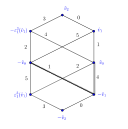
We choose as initial data a shift of (6.52), namely . Its orbit is shown in Figure 8, it consists of the vectors:
| (6.54) |
and their opposite, and one can check that the orbit is complete.
6.4.2 Spectral curve
There exists a polynomial of degree:
| (6.55) |
such that for are the solutions of . Let us describe its symmetries:
-
The orbit is stable under the isometry . Hence: iff . But contrarily to § 6.3, the orbit is not pointwise invariant under , so it will not be simpler to study the quotient by the involution .
-
The orbit is stable under , so iff .
-
The palindrome symmetry adds that iff .
Since is a single segment, we count (Lemma 3.10) a genus for the Riemann surface obtained from the skeleton graph. Since a rational parametrization does not exist, there is no shortcut and we have to determine the coefficients of . It must have the Puiseux expansions at and in a sheet :
| (6.56) |
where:
They give rise to the slopes and in the Newton polygon of – overall sign chosen so that they leave the polygon on their left –, and the leading coefficients in (6.56) give the roots of the slope polynomials. We observe that all leading coefficients are roots of unity, up to a homogeneity factor of (resp. ) on the facets with (with ). Absorbing this homogeneity factor in the definition, the slope polynomials are thus cyclotomic:
| (6.57) |
We deduce that:
| (6.58) |
and the slopes must be arranged in a sequence such that they form the boundary of a convex polygon. Starting with South-East steps – belonging to facets with – and following the counterclockwise order, this sequence reads:
| (6.59) | |||
Let us put the lexicographic order on the monomials : first compare the degree in , then the degree in . We infer from (6.59) that the minimal monomial appearing in is , and we can normalize so that it appears with coefficient . Then, following the slope polynomials along (6.59) determines completely the coefficients of on the boundary of the Newton polygon, see Figure 9.
With this normalization, the symmetry of the orbit and the palindrome symmetry of our solution imply:
| (6.60) |
If we set and , it remains to find coefficients inside the Newton polygon of :
| (6.61) | |||||
If the ’s were generic, the curve of equation would have genus . But according to (3.31), our solution must achieve genus , and the ’s should be determined as functions of .
First, we try to reduce the number of parameters. Let us give names to the first few moments of the equilibrium measure:
| (6.62) |
The ’s are function of and their definition implies when . By construction we have:
| (6.63) |
Expanding this polynomial when , we can identify the ’s in terms of the ’s, and the form (6.61) also imposes constraints on the ’s. We find that all ’s and ’s can be eliminated except and .
If and were generic, the curve of equation would have genus , but the solution we look for has genus . It means that the curve has singular points, and they will come in two orbits under the symmetries and . Let us exploit the symmetries by setting:
| (6.69) |
and eliminate and to get a polynomial equation :
| (6.70) | |||||
This curve should have two singular points, i.e. there exists and such that:
| (6.71) |
Solving explicitly these algebraic constraints is complicated, but we do expect that they select a finite number of solutions for and . Eventually, the (hopefully unique) appropriate branch should be chosen by requiring that the coefficients of expansion are rational numbers.
6.4.3 Two-point function
A rational solution of the linear equation with right-hand side exists for , otherwise we have a log. The outcome of the computation of the residue vectors of the particular solution for the primitive of the two-point function is:
| (6.72) | |||||
We order the vectors of the orbit described in (6.54) as follows:
in order to write down the matrix of singularities . Substracting a matrix filled with:
| (6.73) |
we find the sparse part given in Appendix C. It has only entries, and there are atmost non-zero entries in the same row.
6.5
| (6.74) |
The dynamics are generated by:
| (6.75) |
and the multiplication by is an operator of rank . The orthogonal projections of the canonical basis on its image is:
| (6.76) |
If we define a new basis of :
| (6.77) |
the root system has a Cartan matrix:
| (6.78) |
We recognize1212 12 Let us give some explanation about the introduction of the ’s. The matrix of scalar products can be directly read off , and it is easy to check that it is definite positive. This implies that is a finite root system, so must be of the form ADE. We already know the rank here, so it does not leave much choice for . Then, there is a part of guess to define a basis which puts the Cartan matrix in standard form. the Cartan matrix of the root system , where ’s play the role of the simple roots labeled according to Figure 10.
6.5.1 Minimal orbits
Deleting the root generates a maximal sub-root system, of type . Therefore, the order of the minimal orbit is:
| (6.79) |
A vector with minimal orbit can be obtained as where is orthogonal to all ’s except . Using the matrix (6.78) containing the , we can write down those equations and solve them. We find a generator:
| (6.80) | |||||
and thus:
| (6.81) |
The orbit of consists of the following vectors and their images under the shift , which make in total vectors. We indicate in the second column the size of the -orbit.
| (6.82) |
One can check that the orbit is complete.
There is a polynomial equation of degree in , whose solutions are precisely the for the orbit of . Let us describe its symmetries:
-
The orbit is stable under , hence iff .
-
The palindrome symmetry gives iff .
Since is a segment, we find a Riemann surface of genus .
6.5.2 Spectral curve
The formulae applied to the orbit (6.82) determine the list of slopes of the Newton polygon of , and the list of slope polynomials:
| (6.83) |
We can then read off the coefficients on the boundary of the Newton polygon (see Figure 11). The degree in is given by:
| (6.84) |
But the -symmetry of the orbit implies:
| (6.85) |
and we know:
| (6.86) |
The residual symmetry and the palindrome symmetry give:
| (6.87) |
The proportionality coefficients have been found by checking the coefficients on the boundary of the Newton polygon. This gives us a polynomial involving unknown coefficients inside the Newton polygon:
| (6.88) | |||||
where the are completed by symmetry (6.87). For generic ’s, the equation defines a curve of genus , but the solution we look for achieves genus . By construction, we have:
| (6.89) |
If we write the expansion at of our solution:
| (6.90) |
then plug it in , we can identify the ’s in terms of the ’s. The constraints on the shape of the Newton polygon and the symmetry of its coefficients allows a linear elimination of all ’s except of them: , and and ; the expression of the ’s is then given in Appendix D.
To determine the remaining ’s in terms of , one has in principle to impose the existence of enough singular points – modulo the symmetries and – to lower the genus down to . This yields algebraic equations, that we were not able to write down given the length of the expressions. We expect – although we cannot prove before writing them down – that these equations have a finite number of solutions, and among those, one can hope – again without proof – that there is a unique one such that when and such that the coefficients of Taylor expansion in are rational numbers. The solution we seek for has all this property, and since we proceeded by necessary conditions, we know that at least one such solution exists.
6.5.3 Two-point function
We can find a rational solution of the linear equation with right-hand side for
, and a solution with a log otherwise. We find residue vectors:
where . On the orbit described above, we find that the plain part of the matrix of singularities is:
| (6.91) |
and the sparse part is a -valued matrix stored in a maple file available on request. Its entries are and in the matrix in front of each there are exactly of them per row (or column) are non zero. Some and could cancel to make a , so we guess that the curve is a -fold cover of a rational curve, which should actually be the quotient curve by the symmetries and .
6.6 : Poincaré spheres
| (6.92) |
The generator of the dynamics is:
| (6.93) | |||||
The subspace has dimension , and it is spanned by the orthogonal projections on of canonical basis:
| (6.94) | |||||
and for . The family below defines a basis of :
| (6.95) |
in which the Cartan matrix of reads:
| (6.96) |
We recognize the Cartan matrix of the root system , and the ’s play the role of the simple roots labeled as in Figure 12. The roots generated by the ’s under action of the Weyl group are the elements of the form:
| (6.97) |
The simple roots can be represented in the standard form:
| (6.98) |
where the now form an orthonormal basis, expressed in terms of the canonical basis in Appendix E.1.
6.6.1 Minimal orbit
generates a maximal1313 13 The order of the Weyl group of is . If we delete instead of , we obtain a root system of type , whose Weyl group has order ; if we rather delete , we obtain a root system of type , whose Weyl group has order . All other choice of roots to delete disconnect the Dynkin diagram and lead to smaller Weyl group. So, the maximal sub-root lattice of has type . sub-root system, which is of type . We can find a vector of minimal orbit as where is orthogonal to all ’s except . It is easy using (6.98) to get the decomposition of a generator on the orthonormal basis of ’s:
| (6.99) |
and the formulae in Appendix E.1 allows its rewriting in terms of the canonical basis:
| (6.100) |
Then, the vector:
| (6.101) |
has an orbit of minimal order, equal to:
| (6.102) |
We find that the orbit is stable by the shift and the involution . This allows the decomposition of into orbits generated by the following vectors, and their opposites. The size of the orbits are displayed in the second column.
The in the last line means that , so we do not need to include the orbit of when describing the other part of the orbit via . One can check that the orbit is complete.
6.6.2 Spectral curve
There exists a polynomial equation of degree in , whose solutions are the for . The symmetries and or the orbit, as well as the palindrome symmetry of our solution, imply:
| (6.103) |
We obtain according to Lemma 3.10 a Riemann surface of genus . The computation of for all elements of the orbit described above gives the list of slopes and slope polynomials:
| (6.104) |
Since all slopes are of the form , the degree of the slope polynomials give the multiplicity of the corresponding slope belonging to the facet . Those of the facets form an identical set of slopes and slope polynomials thanks to the palindrome symmetry. We learn that must have degree in and its minimal monomial is . Choosing its coefficient to be and following the slope polynomials then determine the coefficients on the boundary of the Newton polygon of (Figure 13). Enforcing the symmetries yields:
| (6.105) |
and:
| (6.106) |
We count that depends on independent coefficients in the interior of the Newton polygon. If they were generic, the plane curve of equation would have genus 2949 (this is the total number of points in the interior of the Newton polygon), but our solution must achieve genus .
By construction, we have:
| (6.107) |
If we write the expansion at of our solution:
| (6.108) |
then plug it in and use the information – shape and symmetries (6.106) – on its Newton polygon, we find that can entirely be expressed in terms of the moments , , , which are however not specified.
6.6.3 Two-point function
We can find a rational solution of the linear equation with right-hand side for
, and a solution with a log otherwise. We find residue vectors:
| (6.109) | |||||
where , while is a vector having huge rational coefficients with huge denominator that we do not reproduce here. Nevertheless, the matrix of singularity for the orbit described above is not so complicated. We identify its plain part as:
| (6.110) |
and its sparse part has entries . And in each row of , there are exactly non-zero entries. This is larger than the covering of degree that we get by dividing out by the symmetries.

6.7
| (6.111) |
The dynamics are generated by . The matrix model is actually the model [35] with a log-square potential, its saddle-point equation is:
| (6.112) |
is found to be the affine Weyl group , while is the Weyl group , and up to rescaling the finite orbit is and has order .
Since (6.112) is very simple, we present a direct solution. The simplest particular solution of (6.112) involves a log-cube, so we prefer to introduce as explained in § 5.1.2:
| (6.113) |
which solves, for any :
| (6.114) |
Thus, has no discontinuity, and given the growth and symmetries of , it must be of the form:
| (6.115) |
Since has a discontinuity on only, the numerator must be a perfect square, hence an answer of the form
| (6.116) |
for some constants and . Notice that this function is odd/odd with respect to the symmetries /, because the determination1414 14 If we were choosing signs so that the squareroot is odd/odd, we find that the right-hand side of (6.114) must be , which is a contradiction.. The result can be integrated once:
| (6.117) |
and the answer is of the form:
| (6.118) |
where and are constants to determine, and we introduce the elliptic integrals
| (6.119) |
and:
| (6.120) |
Since , we must have . Since we have the asymptotic behavior when :
we must impose a relation between and :
| (6.121) |
Next, we have to match the first equation of (6.114). Using the functional relations:
| (6.122) |
we deduce the value:
| (6.123) |
where all complete elliptic integrals are evaluated at , except for E evaluated at . Eventually, the position of the cut is determined implicitly by the normalization of the spectral density:
| (6.124) |
6.7.1 -point function
We find residue vectors:
| (6.125) |
Taking as initial vector, the matrix of singularity can be decomposed:
| (6.126) |
and we find . Therefore, if we introduce a uniformization variable for the curve:
| (6.127) |
the two-point function reads:
| (6.128) |
6.8
| (6.129) |
The dynamics are generated by:
| (6.130) |
has dimension , and it is spanned by the orthogonal projections of on :
| (6.131) | |||||
| (6.132) | |||||
| (6.133) |
So, iff . The Cartan matrix of the root system in the basis is:
| (6.134) |
We recognize the Cartan matrix of the root system , where plays the role of the simple roots, and its Weyl group is the symmetric group in elements. Deleting (or ) gives a maximal sub-root system, of type . A generator of is:
| (6.135) |
Its image is:
| (6.136) |
The orbit of is a cycle of order , the two other vectors begin and .
We may also consider the ”root system” . Its ”Cartan matrix” in the canonical basis is:
| (6.137) |
hence is the affine root system of type . By construction, its Weyl group is : it is therefore the symmetry group of the tiling of the plane by equilateral triangles.
6.8.1 Spectral curve
We set:
| (6.138) |
which solves, for any , the linear equation:
| (6.139) |
The discussion of § 6.8 tells us that can be analytically continued to an analytic function a Riemann surface with sheets. The value of in the other sheets is and , and its singularities follow from those of listed in § 5.1.2. We therefore have a polynomial equation , but the symmetry tells us that, if is a solution, then is a solution, and is a solution. This information, and the order of singularities of , prescribe the following form:
| (6.140) |
where and are degree polynomials.
6.8.2 -point function
We find the residue vectors:
| (6.141) |
The matrix of singularities for the orbit of can be decomposed as:
| (6.142) |
and we find .
6.9
| (6.143) |
The dynamics are generated by:
| (6.144) |
has dimension , and it is spanned by the orthogonal projections of on :
| (6.145) |
So, iff . A basis of is given by , and the Cartan matrix of the root system in this basis is:
| (6.146) |
hence is the root system of type . Its Weyl group is isomorphic to the symmetric group in elements. Deleting (or ) gives a maximal sub-root system, of type . A generator of is:
| (6.147) |
Its image is:
| (6.148) |
The orbit of is a cycle of order , containing the vectors , and .
We may also consider the ”root system” . Its ”Cartan matrix” in the canonical basis of is:
| (6.149) |
hence is the affine root system of type , and is the corresponding affine Weyl group.
6.9.1 Spectral curve
6.9.2 -point function
We find the residue vectors:
| (6.153) |
The matrix of singularities for the orbit of can be decomposed in a plain matrix and a sum of permutation matrices:
| (6.154) | |||||
and again higher ’s vanish.
6.10
| (6.168) |
The dynamics are generated by:
| (6.169) |
has dimension , and is generated by the orthogonal projections of on :
| (6.170) |
So, iff . for defines a basis of , and the Cartan matrix of the root system reads in this basis:
| (6.171) |
We recognize the Cartan matrix of the root system. Deleting (or ) gives a maximal sub-root system, of type . A generator of is:
| (6.172) |
Its image is:
| (6.173) |
The orbit of is a cycle of order , containing the vectors for .
We may also consider the ”root system” . Its ”Cartan matrix” in the canonical basis of is:
| (6.174) |
hence is the affine root system of type , and is the corresponding affine Weyl group.
6.10.1 Spectral curve
6.10.2 -point function
We find residue vectors:
| (6.178) | |||||
| (6.179) |
We label as follows the vectors of the orbit of :
| (6.180) |
and we find a matrix of singularity:
| (6.182) |
with:
where is the matrix with ’s on the antidiagonal. The higher ’s vanish.
7 Topological recursion
7.1 General result
It was shown in [14] that the asymptotic expansion of multidimensional integrals of the form (2.1) is governed by the topological recursion introduced in [22].
We denote the spectral curve : it is the Riemann surface on which (for a certain set of ) has been analytically continued on . We denote the analytic continuation. is equipped with two points , and a covering , such that (the endpoints of the support of the equilibrium measure) are simple branchpoints. We introduce the -form on defined by:
| (7.1) |
It has simple zeroes at .
Definition 7.1
Let be the deck transformation, defined in the neighborhood of : it is the holomorphic map such that and for .
The spectral curve is also equipped with a bidifferential having (among possible other singularities) a double pole at coinciding points with coefficient and no residues. is the initial data needed to compute the large expansion of all correlators.
Definition 7.2
We define the recursion kernel:
| (7.2) |
The recursion kernel has a simple pole at .
Theorem 7.3
For , the differential forms are computed recursively on by the formula:
| (7.3) |
The proof of this result follows directly from [14, Section 1 and 3].
Once and are known, this formula provides an algorithm to compute the Chern-Simons free energies, and the perturbative expansion of the colored HOMFLY of fiber knots in Seifert spaces. For lens spaces, the equation of the spectral curve was a polynomial in , and that implied that the perturbative invariants were polynomials in . In particular, they did not have any singularity for in the complex plane.
The situation is different for the other Seifert spaces , since the interior coefficients of the equation of the spectral curves are in general algebraic function of . We have seen for instance in the case that the spectral curve was polynomial in given by (6.14). It would be interesting to give an interpretation of this ”algebraic change of variable” as a non-trivial mirror map in the context of topological strings ( should be in correspondence with some Kähler parameter).
We will now derive a few formulas and consequences of our results for . In particular, in § 7.2-7.3 we obtain hypergeometric formulas for the planar limit of the HOMFLY-PT of fiber knots generalizing those given in [17] for torus knots. We also establish in § 7.2.2 arithmetic properties of the all-genus perturbative invariants when is even.
7.2 , even
7.2.1 Disk invariants
The spectral curve is given in (6.13) The expansion when (i.e. in the sheet ) is of the form:
| (7.4) |
We compute by Lagrange inversion:
| (7.5) |
where we have defined a new coordinate , which is such that in the regime we are interested.
Each term can be explicitly computed and gives a Laurent polynomial in that can be put in hypergeometric form:
| (7.7) | |||||
For instance:
| (7.8) |
for the knot going along an exceptional fiber of order . Similar formulas involving sum of two polynomial hypergeometric can be found for for any . Those formulae can be seen as generalizations of the large limit of Rosso-Jones formula for torus knots [42].
7.2.2 All-genus invariants
Theorem 7.4
For any , and genus , we have:
| (7.9) |
Poles may occur at .
Theorem 7.5
The endpoints of the singularity locus of – seen as a function of – occur at . A more precise description arise follows from (7.31).
Proof. Applying Theorem 7.3 requires the compute the coefficients of expansion around the ramification points of several quantities. We only focus on the arithmetic properties of those coefficients. It is convenient to introduce the coordinate :
| (7.10) | |||||
| (7.11) |
Then, the two ramification points so that are:
| (7.12) |
Since , we may write:
| (7.13) |
Deck transformations. The equation:
| (7.14) |
defines a unique formal power series . The coefficients are polynomials in and . Since , we deduce that . The singularities of come from zeroes of . The latter only occur at and with:
| (7.15) |
Spectral density. In the recursion kernel, we meet the quantity:
| (7.16) |
to expand in formal powers series when . A priori, we have , but we also observe that:
| (7.17) |
Thus, is odd in , i.e. . In particular, we have:
| (7.18) |
and the other have singularities at singularities of . These singularities occur at , or or which amounts to .
Two-point function. The two point function was given in (6.24):
| (7.19) |
We need its expansion:
-
when is a free variable, and . The coefficients of expansion are in . The singularities in involve denominators which are powers of and .
-
when and . The coefficients of expansion are in .
No new singularity occur in the -plane.
Topological recursion. With the formula of Thm. 7.3, the above series allows, after a sequence of nested residues at and , the computation of:
| (7.20) |
Since we sum the residues at the two ramification points at each step, the result must be even of . Hence, it will be a rational function in the variables , which can be themselves rewritten as polynomials in:
| (7.21) |
Subsequently:
| (7.22) |
Lagrange inversion. All perturbative invariants can be extracted from the expansion of when as a power series involving (see § 4.4), as done in § 7.2.1 for the disk invariants. The can be decomposed with coefficients in in the basis of:
| (7.23) |
for and . The latter can be expanded:
| (7.24) |
with:
| (7.25) | |||||
A singularity in occurs when is such that one of the term in (7.25) which is not explicitly a has a pole at , that is when , or , or . Therefore, the singularities of in the -plane occur when .
Combining all results, we find that belongs to . Moreover, the denominators can only contain powers of and . We remind the relation (6.36) between and the Chern-Simons variable :
| (7.26) |
Therefore, the list of singularities of the perturbative colored HOMFLY in the -complex plane occur when is equal to:
where:
| (7.27) |
This list is complete, except that must be removed since by construction, we know that invariants are when .
Free energies. The can be obtained from by (2.22). For , the topological recursion computes in terms of the two-point function. We therefore need to study the arithmetic properties of the quantities:
| (7.28) |
where we integrate around the cut and . We have:
| (7.29) | |||||
The derivatives can be explicitly computed, and we find:
| (7.30) |
Besides, the three rational functions of appearing in this expression are odd if is odd (resp. even if is even). It is clear from (7.29) that the singularities of as a function of only occur when the singularities of as a function of approach the cut . The quantities are linear combinations of with coefficients in , and the result should be even in – since and play a symmetric role. And, we remind that . Therefore:
| (7.31) |
where:
| (7.32) |
The location of singularities of the free energies can easily be deduced.
7.3 , odd
7.3.1 Disk invariants
The spectral curve is given in (6.35). Checking the behavior (5.9)-(5.10) shows that corresponds to in the sheet labeled by . Therefore, the expansion at those points of in terms of the variable , reads:
By Lagrange inversion, we find:
After a change of variable , this residue can be explicitly computed:
Since is a function of independent of the parity of , we observe the relation:
| (7.33) |
In particular, the planar limit of the HOMFLY-PT of is obtained by taking in (7.3.1). The computation of even powers is very similar, and we get:
| (7.34) | |||
In particular, the planar limit of the HOMFLY of the knot following the fiber of order is obtained by taking :
| (7.35) |
8 Generalization to and Chern-Simons
8.1 The model
For more general gauge groups, Chern-Simons theory on Seifert spaces is described by the following measure on the Cartan subalgebra – identified with :
| (8.1) |
where the product ranges over positive roots. For the series, we had:
| (8.2) |
Now, we would like to address the series:
| (8.3) |
with
| (8.4) |
They correspond to the Lie algebras:
| (8.5) |
We will explain the main points of the analysis of those models, and skip the details which are very similar to the already studied A series.
8.1.1 First rewriting
Let us perform the change of variable with , and put the measure (8.3) in the form:
| (8.6) |
where the potential is:
| (8.7) | ||||
The terms are absent for the A series, and are equal to:
| (8.8) |
And, the pairwise interaction is:
| (8.9) |
for the A series, and:
| (8.10) |
for the BCD series.
8.1.2 Second rewriting
The BCD matrix model can also be rewritten:
| (8.11) |
with:
| (8.12) | |||||
The potential for this model is obtained by including the part of the diagonal terms which are regular:
| (8.13) |
with:
| (8.14) |
and were defined in (8.8). In other words:
| (8.15) |
8.1.3 Observables and symmetries
We observe in (8.3) that individually is distributed like . Therefore, the joint probability density vanishes at , and to find the dominant configuration of (8.3) when of (8.3) via potential theory, it is enough to restrict to even configurations. One can then show uniqueness and off-criticality of the equilibrium measure at least when (see Appendix A.4). We assume in all what follows.
The naive definition of the -point correlators is:
| (8.16) |
with . In order to emphasize later the relation between the A series and series, it is convenient to introduce the symmetrized correlators:
| (8.17) |
By symmetry, we have:
| (8.18) |
and thus for the leading order :
| (8.19) |
Stricto sensu, the existence of an all-order asymptotic expansion of the form:
| (8.20) | |||||
does not follow from the results of [15] since the potential has a log singularity at . It is nevertheless likely that the argument can be generalized for this model. In the remaining, we will take the asymptotic expansions (8.20) as starting point1515 15 From the theory of the LMO invariants, it holds at least as equality of formal series in the variables and (see § 4.2)., with being analytic functions of variables away from a cut . Compared to the expansion (4.18) for the A series, since the log term of the potential contains a corrections (the log terms coming from ), is not expected to have an expansion of parity in .
Our goal is to compute the coefficients of (8.20). We will first write linear functional equations , as well as and . If , the equation for given in § 8.2 below can be derived as a saddle point equation for the Stieltjes transform of the equilibrium measure. For and , the equations are given in § 8.3 and § 8.4 below can be derived from the Schwinger-Dyson equations presented later in § 8.5.1-8.5.3, after pluging the expansion (8.20) and equating the discontinuities of the two sides of the Schwinger-Dyson equations. For this purpose, we will show that the symmetrized correlators satisfy a set of loop equations, which are solved by a version of the topological recursion adapted to the grading in (8.20). This is performed by adapting the tools of [14] to take into account the presence of a symmetry.
8.2 Spectral curves
We first have a look at the equilbrium measure in the model (8.3). We denote the support of the equilibrium measure, emphasizing its dependence in the parameter . We find, for any . The saddle point equation for is obtained as (2.16) was obtained from (2.11). Since it concerns only the leading order when , the only term relevant in the potential is that involving . Notice that here, the joint probability density is singular when and . The second singularity is also relevant since configurations with can occur with . We find, for any :
| (8.21) | |||||
In terms of the symmetrized correlator, we therefore find, for any :
| (8.22) |
For , this equation characterizes the equilibrium measures together with the condition:
| (8.23) |
This is shown by repeating the proof of Corollary 2.2 using the strict concavity proved in Appendix A.4. for the BCD series. Therefore, we deduce, if :
| (8.24) |
In other words, the spectral curve are the same in the B, C, or D series. They are obtained from the spectral curve of the A series upon replacement of by , for which we can use the results of Section 5-6.
8.3 Two-point function
Following the strategy of § 2.4, we can derive the saddle point equation for the leading order of the -point correlator. We find, for any and :
where . This implies the saddle point equation for the symmetrized -point function:
| (8.25) |
Since , the right-hand side is a symmetric function of and , which is transformed into its opposite when .
Let us compare (8.25) with the saddle point equation of the two-point function for the A series: for any and ,
| (8.26) |
Since and this equation characterizes the two-point function with appropriate growth condition at in the cases , we deduce:
| (8.27) |
Remark. The two-point function plays the role of a fundamental solution in the following sense: the function for any choice of function holomorphic near the contour of integration which avoids the cut, is the solution of the functional equation on the cut :
| (8.28) |
for a function holomorphic on satisfying appropriate growth conditions at . It is convenient to introduce:
| (8.29) |
8.4 First correction to the spectral curve
In the A series, the first correction to the spectral curve was of order . In the BCD series, because the potential contains an extra term of order , the first correction is , and is obtained by formally writing down the -dependent saddle point equation for , and collecting the term of order . We find, for any :
| (8.30) |
Given the expression of the right-hand side (8.30), it can be decomposed in partial fraction expansion:
| (8.31) |
Using the remark of § 8.3 and (8.29), we deduce that, if :
| (8.32) |
8.5 Schwinger-Dyson equations
8.5.1 First equation …
The invariance of the partition function under the infinitesimal change of variable yields relations between correlators. Those equations can be derived rigorously by integration by parts. Here, we obtain:
| (8.33) | ||||
We first add the diagonal term to obtain and substract it, which has for effect to cancel the : this is a consequence of vanishing of order of the joint probability density (8.11) when . Adding the terms also gives extra contributions which can be put in the form of a perturbation of the potential. Then, by symmetry between the two terms in the in (8.33), we find:
| (8.34) |
The first term is the expectation value of an analytic function in a neighborhood of the cut, so can be rewritten in terms of a contour integral of .
| (8.35) |
With the goal to compute the integral over , we compute the partial fraction expansion of as a function of :
| (8.36) |
If we rewrite in terms of , we should keep in mind that has poles at which is on the cut. All in all, we find the equation:
| (8.37) |
The first double integral could be perform by picking up residues at and , but this expression is enough for our purposes. For comparison, the first Schwinger-Dyson equation of the model of the A series in terms of its correlators
| (8.38) |
can be written:
| (8.39) |
(8.37) only differs from (8.39) by addition of terms involving , due to the structure of (8.12), and a potential instead of .
8.5.2 …and its symmetrized form
Our next goal is to derive Schwinger-Dyson equation involving the symmetrized correlators only:
| (8.40) | ||||
We denote and the terms involving and in (8.37). We observe that:
| (8.41) |
Therefore, we have:
| (8.42) | ||||
Therefore:
| (8.43) |
Similarly, let us define and consider a summation index with and , and
We compute:
| (8.44) | ||||
Since the sum over contains both and , we find:
| (8.45) | ||||
We observe that in (8.43) (resp. (8.45)) the second term – call it , resp. – is the negative part of the Laurent expansion of (resp. ) at , whereas the first term is regular at . Since we have the equation:
| (8.46) |
this implies that . Then, summing (8.43) and (8.45) gives:
| (8.47) |
In this form, we recognize the Schwinger-Dyson equation of the correlators of the model in the A series, in the potential given by (8.13).
8.5.3 Higher equations
Let be the insertion operator: it computes under the perturbation . We have the properties:
| (8.48) |
Higher Schwinger-Dyson equations involving can be derived by applying the operator to (8.37). One can also define an insertion operator adapted adapted to symmetrized observables: it computed under the perturbation . It has the property:
| (8.49) |
A word of caution: the symmetries (8.18)-(8.19) are only valid when the potential (and its perturbation) are invariant under . Therefore, if we make any use of this relation to transform the Schwinger-Dyson equation, only the application of symmetrized insertion operators is allowed.
8.6 Loop equation and recursive formula
The Schwinger-Dyson equation (8.47) and their analogue is now similar to those treated in [14, Section 3].
If one insert the expansion (8.20) in the Schwinger-Dyson equations and study the discontinuity of both sides, one can prove by recursion on that defined for , satisfies the linear functional equation:
| (8.50) |
if , and (8.22)-(8.25)-(8.30) in the first three cases. One can then establish for that diverges polynomially when approaches the edges of the cut , but is regular at other points, including . This contrasts with the singularity at occuring for , which was due to the log singularity in the potential.
From (8.50) by Schwarz principle, we deduce that can be analytically continued as a meromorphic function on the spectral curve . The spectral curve is equipped with a covering , and with a local involution which exchanges the two sheets at the vicinity of the ramification points. The initial is identified with the physical sheet in this covering. We still denote the preimages ot the two endpoints of the cut in the physical sheet. We introduce the differential -forms on the spectral curve:
| (8.51) |
They are meromorphic with poles at all preimages of the endpoints of the cut in . We also introduce the Cauchy kernel:
| (8.52) |
where is given by (8.29).
Then, following [14, Section 3.7], the Schwinger-Dyson equation – and its higher versions – can be written for any , with the convention that for :
| (8.53) |
where is a holomorphic quadratic differential in in a neighborhood of the image of in , and we have written apart the term which has a simple pole at :
| (8.54) |
There are two differences with the setting of the topological recursion presented in [14]. Firstly, we have an extra term which contains a pole a . This pole thus occurs away from the branchpoints. Secondly, since the potential was perturbed by a term of order , we have all possible powers of for in the expansion of – instead of just for .
We can nevertheless proceed as usual to solve the abstract loop equations. We use the notations:
| (8.55) |
so that we can write:
| (8.56) |
Then, we may recast (8.53) as:
| (8.57) |
with:
| (8.58) |
and:
| (8.59) |
We know that:
| (8.60) |
is holomorphic in a neighborhood of , and satisfy the linear equation (8.50). Here, the poles at those on the image in of the cut. By unicity, (8.60) must vanish. Notice that has a double zero at since the equilibrium measure behaves exactly like a squareroot at the edges of the cut (this is the off-critical property). So, we find that has the same property, and we deduce that the right-hand side of (8.57) does not contribute to the residue at in (8.60), which yields:
| (8.61) |
This is a recursion on . We observe that this recursion is universal : the only way the B,C or D series matters is through the value of for which are used at every step. These values are given in equations (8.24)-(8.27)-(8.32).
This formula is a recursion on , and is the generalization for the Chern-Simons theory of the topological recursion found in Theorem 7.3 for the Chern-Simons theory.
9 Numerical estimates of equilibrium distributions
by Alexander Weisse
9.1 Markov chain Monte Carlo
The probability measure
| (9.1) |
describes a statistical system of classical particles with coordinates , and is its partition function. We are interested in the equilibrium distribution of the particle coordinates, , which can be estimated from the large- limit of the empirical measure
| (9.2) |
The phase space of such a many-particle system is far too large to be summed up completely or to be explored by naively selecting random configurations. Instead, the standard simulation technique is a Monte Carlo algorithm with importance sampling [8]. It is based on a suitable Markov chain process which converges to the measure . A Markov chain is a stochastic process in which a set of random variables is updated to a new configuration with a probability that depends only on and , but not on the earlier history of the process,
| (9.3) |
The process converges to the distribution , if the transition probability fulfills the condition of detailed balance,
| (9.4) |
A good choice for such a transition probability is the classic Metropolis algorithm [39],
| (9.5) |
For large the probability ratio in the above expression is a ratio of two very small numbers. Since this is difficult to handle numerically, we rewrite in terms of an energy function ,
| (9.6) | ||||
| (9.7) |
and use the energy difference of two configurations, , to evaluate the transition probability . In our simulations we use local updates, i.e., we propose a random change of one coordinate . If this change lowers the energy, , we always accept the update. If the change increases the energy, we accept the update only with probability . We loop over all coordinates and repeatedly try updates for each of them.
After a certain “warm-up” period the Markov process usually reaches equilibrium with a stable coordinate distribution , which we can measure in a histogram. We call the successful Metropolis update of coordinates a Monte Carlo step. For the results presented below we typically performed warm-up steps and measurement steps.
9.2 Torus knots
The reliability of the Monte Carlo approach can be tested by first considering the special case of the general model (2.1), which has been studied earlier in the context of torus knots,
| (9.8) | ||||
Here, and are two coprime integers labeling the knot, and is a free parameter. The equilibrium distribution of this model is determined by the equations [17]
| (9.9) | ||||
| (9.10) |
where the boundaries of the domain of (the branch points) are given by the two zeros of . In Figure 14 we compare this exact result to the numerical data obtained by simulating particles. The agreement is almost perfect: only the edges of the distribution are slightly softened due to the finite number of particles.
9.3 Seifert fibered spaces
9.3.1 Rôle of strict convexity
In § 4.1.3 it was pointed out that an important geometric invariant of the Seifert space is the orbifold Euler characteristic
| (9.11) |
and is also expected to have an influence on the properties of the statistical model (2.1). The long distance behavior of the pairwise interaction is determined by ,
| (9.12) |
For , is always repulsive and strictly convex, and a unique equilibrium measure exists and can be calculated. For , unfortunately, the analytic methods cannot be applied, and it was unclear whether a unique exists and how it looks like.
We therefore performed numerical simulations for both situations, and , in the case . The statistical model (2.1) then specializes to
| (9.13) | ||||
where are three integer parameters and is real and positive.
The Monte Carlo simulations with particles suggest that a unique equilibrium measure exists independently of the sign of . In Figure 15 we show data for the parameter sets , and . The first set fulfills the condition and leads to a unique equilibrium distribution . However, the simulations converge equally well for the other parameter sets with . The shape of the resulting equilibrium distributions differs only marginally from the first case. The small oscillations near the edges of the distributions and the softening of the edges are caused by the finite particle number. For we expect smooth distributions which at the boundaries of the domain vanish like a half-integer power of .
We also studied the scaling of with increasing , i.e., with decreasing strength of the potential . For the interaction is always repulsive and the expansion of the particle distribution is limited by the potential (and thus depends on ). For the interaction is repulsive at short distance but attractive at long distance. Therefore, for large enough , it is plausible that the support of the particle distribution reaches a limit which is independent of . In Figure 16 we illustrate the scaling of for the three cases , and , which correspond to positive, vanishing and negative , respectively. For and large enough the width of the distribution scales like , whereas it seems to approach a constant for . For the scaling seems to be weaker than the first guess . This could be due to logarithmic corrections.
9.3.2 The case
In this and the remaining sections we compare analytic results for the model (9.13) with numerical data. For the case with even the characteristic and the equilibrium density is given by
| (9.14) |
where and are solutions to the equations (see § 6.2):
| (9.15) | ||||
with
| (9.16) |
In Figure 17 we compare this result to simulation data for particles and . The agreement is excellent. Note that we plot the densities as a function of rather than .
9.3.3 The case
For the case with odd the equilibrium density,
| (9.17) |
can be obtained analytically from
| (9.18) | ||||
where
| (9.19) |
In Figure 18 we compare the analytical result to simulation data for particles and . Again, the agreement is excellent.
9.3.4 The case
The case admits only a partial analytical solution. The equilibrium density again corresponds to a branch cut,
| (9.20) |
but the equations defining the Riemann surface contain two parameters and whose dependence on the interaction as yet could not be determined (see § 6.4). In terms of the variables and with , the branch points fulfill:
| (9.21) | ||||
Taking and as adjustable parameters, we can easily solve these equations for and and fit the solution of to the numerical data. For all values of we can perfectly match the simulation results, see Figure 19 below. The corresponding parameters and are given in the legend.
9.3.5 The gauge groups SO and Sp
In Section 8 the generalization of the statistical model (2.1) to gauge groups and was studied, and it was shown in § 8.24 that in the limit the corresponding equilibrium distributions for parameter are given by the data with parameter . One noticeable difference between the and densities (BCD series) and the density (A series) is a finite-size correction taking the form of a Dirac peak of order at (see (8.32)).
To verify these predictions, which were derived for the convex interaction , and to analyze whether they hold for , we performed numerical simulations for various parameter sets and increasing particle numbers . In Figure 20 we show equilibrium densities for three parameter sets with positive, zero and negative . The densities for the B, C, and D cases at agree very well with the data for the A case at . Only in the vicinity of we observe the predicted finite-size correction. The total mass of the Dirac peak is negative for the cases B and C, and positive for the case D, but its absolute amplitude is the same for all BCD cases. In Figure 21 we analyze the scaling with increasing particle number . Clearly, doubling reduces the -peak by a factor . These observations are in agreement with (8.15)-(8.32), which predicts for the following masses for the Dirac peak:
| (9.22) |
9.4 Conclusion
The matrix models considered in this work can reliably be simulated with Monte Carlo methods. The numerical data has been used to verify analytic results and to gain further insight into cases that elude an analytic solution.
Appendix A Proofs of Section 2
A.1 Proof of Lemma 2.1
Let with compact support. We compute:
| (A.1) | |||||
with and is the Heaviside step function. We compute the Fourier representation of , in the distributional sense:
| (A.2) | |||||
The Fourier transform of the measure is denoted:
| (A.3) |
It is a function of because is the difference of two probability measures with compact support, and since , we have when . being real, we also have . Using the representation (A.2) in (A.1), we find:
| (A.4) | |||||
where:
| (A.5) |
The same computation with will result in replacing by , hence the result of Lemma 2.1:
| (A.6) |
A.2 Proof of Corollary 2.2
The cotanh function has the expansion:
| (A.7) |
It follows that:
| (A.8) |
Therefore, a necessary condition for the positivity of is . We immediately observe that is always definite positive when when or . When , it is only positive for a certain region of parameters . Its description is not easy, but since is decreasing, we know that gives a positive , then with gives a positive . For the models related to Seifert spaces, we are only interested in taking integer values. We can immediately exclude the uples with . Then, the list of uples satisfying to with is finite, and positivity can be checked directly case by case:
-
For the cases , we find:
(A.9) -
For with , it is enough to check positivity in the case and use the monotonicity property stated above. We have for :
(A.10) -
For , we have:
(A.11) -
For , we have:
(A.12) -
For , we find:
(A.13)
This concludes the proof of Corollary 2.2.
A.3 Proof of Theorem 2.3
Proof. The effective potential is:
| (A.14) |
where:
| (A.15) |
We compute:
| (A.16) | |||||
We have introduced . If , we have ensuing from and:
| (A.17) |
Therefore, is a concave function, hence is a convex function for any fixed . This implies that it must achieve its minimum in a connected set, i.e. the support must be a segment.
We claim that the density of vanishes exactly like a squareroot at the edges. By analyticity arguments, we know that it behaves at any edge of the support, for some integer and irrelevant constant , but we claim . Indeed, the effective potential behaves like when from the exterior of the support. However, from the expression, the effective potential is in the variable not belonging to the support, and:
| (A.18) |
Since we have shown that is concave:
| (A.19) |
which is only compatible with .
In case the equilibrium measure is unique, is even, so its support is of the form , and after the change of variable, we find that the support of is . In case the equilibrium measure is not unique, and denote the support of a given equilibrium measure . Denote the image of under . The characterization of equilbrium measures shows that any convex combination is an equilibrium measure. By the previous argument its support is connected, therefore , i.e. the support of any equilibrium measure contains .
A.4 For and gauge groups
We have to repeat the analysis of § A.1 for the quadratic form:
| (A.20) | |||||
over measures which are the difference of two even probability measures. We compute as in (A.1):
| (A.21) | |||||
Therefore:
| (A.22) |
Since is even, its Fourier transform is real and therefore, is definite positive iff (A.6) is strictly convex. In that case, one can prove repeating § A.3 that the equilibrium measure for the BCD series is supported on segment and behaves exactly as a squareroot at the edges.
Appendix B Finite subgroups of
We are studying functional relations with the values of and on both sides of a cut are related to values of at , where is a Möbius transformation, and the ’s involved generate a finite subgroup of . The list of possibilities, and has an ADE classification: up to conjugation, must be either cyclic, dihedral, or one or the three polyhedral groups.
-
, cyclic group of order . Generated by – case.
-
, dihedral group of order . Generated by and – case.
-
, tetrahedral group, order . It is also the alternate subgroup of . It is generated by and (order ) – case.
-
, octahedral group, order . It is generated by and – case.
-
, icosahedral group, order . It is generated by , , and , with and is its complex conjugate (order ) – case.
Appendix C Case : matrices of singularities
We have with:
Appendix D case: polynomial equations
The coefficients in the polynomial (see (6.88)) for the spectral curve for can be expressed solely in terms of the four coefficients for .
| (D.1) | |||||
Appendix E case: additional formulas
E.1 The basis of ’s
In § 6.6, we have found a orthonormal basis of . Its expression in terms of the canonical basis of is:
| (E.1) | |||||
where is a linear operator reverting the order of the canonical basis, and is the shift:
| (E.2) |
E.2 Two-point function
with the following coefficients:
References
- [1] D. Bar-Natan, S. Garoufalidis, L. Rozansky, and D.P. Thurston. The Aarhus integral of rational homology -spheres I: a highly non trivial flat connection on . Selecta Mathematica, 8(3):315–339, 2002. q-alg/9706004.
- [2] D. Bar-Natan, S. Garoufalidis, L. Rozansky, and D.P. Thurston. The Aarhus integral of rational homology -spheres II: invariance and universality. Selecta Mathematica, 8:341–371, 2002. math.QA/9801049.
- [3] D. Bar-Natan, S. Garoufalidis, L. Rozansky, and D.P. Thurston. The Aarhus integral of rational homology -spheres III: the relation with the Le-Murakami-Ohtsuki invariant. Selecta Mathematica, 10:305–324, 2004. math.QA/9808013.
- [4] D. Bar-Natan and R. Lawrence. A rational surgery formula for the LMO invariant. Israel J. Math., 140:29–60, 2004. math.GT/0007045.
- [5] C. Beasley. Localization for Wilson loops in Chern-Simons theory. 2009. hep-th/0911.2687.
- [6] C. Beasley and E. Witten. Non-abelian localization for Chern-Simons theory. J. Diff. Geom., 70:183–323, 2005. hep-th/0503126.
- [7] A. Beliakova and T.T.Q. Lê. On the unification of quantum -manifold invariants, volume 46, pages 1–21. World Scientific, New Jersey-London-Singapore-Beijing-Shanghai-Kong Kong-Taipei-Chennai, 2012. math.GT/1106.6298.
- [8] K. Binder and D.W. Heermann. Monte Carlo Simulation in Statistical Physics – An Introduction. Graduate Texts in Physics. Springer, Berlin, 5 edition, 2010.
- [9] M. Blau and G. Thompson. Chern-Simons theory on -bundles: abelianisation and -deformed Yang-Mills theory. JHEP, 0605(003), 2006. hep-th/0601068.
- [10] M. Blau and G. Thompson. Chern-Simons theory on Seifert manifolds. JHEP, 33, 2013. hep-th/1306.3381.
- [11] G. Borot, J. Bouttier, and E. Guitter. Loop models on random maps via nested loops: case of domain symmetry breaking and application to the Potts model. J. Phys. A, special issue in honor of F. Wu, 2012.
- [12] G. Borot, A. Brini, and A. Klemm. Large rank dualities for Chern-Simons theory on quotients of -sphere.
- [13] G. Borot, B. Eynard, M. Mulase, and B. Safnuk. A matrix model for simple Hurwitz numbers, and topological recursion. J. Geom. Phys., 61(26):522–540, 2010. math-ph/0906.1206.
- [14] G. Borot, B. Eynard, and N. Orantin. Abstract loop equations, topological recursion, and applications. 2013. math-ph/1303.5808.
- [15] G. Borot, A. Guionnet, and K. Kozlowski. Large- asymptotic expansion for mean field models with Coulomb gas interaction. 2013. math-ph/1312.6664.
- [16] V. Bouchard, A. Klemm, M. Mariño, and S. Pasquetti. Remodeling the B-model. Commun. Math. Phys., 287:117–178, 2009. hep-th/0709.1453.
- [17] A. Brini, B. Eynard, and M. Mariño. Torus knots and mirror symmetry. Annales Henri Poincaré, 2012. hep-th/1105.2012.
- [18] P. Deift. Orthogonal polynomials and random matrices : a Riemann-Hilbert approach. AMS, New York, 1998. Courant Institute of Mathematical Sciences.
- [19] B. Eynard. Gravitation quantique bidimensionnelle et matrices aléatoires. 1995. Thèse de doctorat, Université Paris VI (1995).
- [20] B. Eynard and C. Kristjansen. Exact solution of the model on a random lattice. Nucl. Phys. B, 455:577–618, 1995. hep-th/9506193.
- [21] B. Eynard and C. Kristjansen. More on the exact solution of the model on a random lattice and an investigation of the case . Nucl. Phys. B, 466:463–487, 1996. hep-th/9512052.
- [22] B. Eynard and N. Orantin. Invariants of algebraic curves and topological expansion. Commun. Number Theory and Physics, 1(2), 2007. math-ph/0702045.
- [23] B. Eynard and N. Orantin. Computation of open Gromov-Witten invariants for toric Calabi-Yau -folds by topological recursion, a proof of the BKMP conjecture. 2012. math-ph/1205.1103.
- [24] P. Freyd, D. Yetter, J. Hoste, W.B.R. Lickorish, K. Millett, and A. Ocneanu. A new polynomial invariant of knots and links. Bull. Amer. Math. Soc., 12:239–246, 1985.
- [25] S. Garoufalidis and T.T.Q. Lê. Is the Jones polynomial of a knot really a polynomial ? J. Knot Theory Ramifications, 15:983, 2006. math.GT/0601139.
- [26] S. Garoufalidis, T.T.Q. Lê, and M. Mariño. Analyticity of the free energy of a closed 3-manifold. SIGMA, 4(080), 2008. math.GT/0809.2572.
- [27] M. Geck and G. Pfeiffer. Characters of finite Coxeter groups and Iwahori-Hecke algebras. Number 21 in London Mathematical Society Monographs. Oxford Science Publications, 2000.
- [28] R. Gopakumar and C. Vafa. On the gauge theory/geometry correspondence. Adv. Theor. Math. Phys., 3:1415–1443, 1999. hep-th/9811131.
- [29] N. Halmagyi and V. Yasnov. The spectral curve of the lens space matrix model. 2003. hep-th/0311117.
- [30] V.F.R. Jones. Polynomial invariants of knots via von Neumann algebras. Bull. Amer. Math. Soc., 12:103–111, 1985.
- [31] E. Kalfagianni and X.S. Lin. The HOMFLY polynomial for links in rational homology 3-spheres. Topology, 38(1):95–115, 1999. math.QA/9509010.
- [32] J. Källén. Cohomological localization of Chern-Simons theory. JHEP, (8):1–32, 2011. hep-th/1104.5353v2.
- [33] A. Kapustin, B. Willett, and I. Yaakov. Exact results for Wilson loops in superconformal Chern-Simons theories with matter. JHEP, (1003:089), 2010. hep-th/0909.4559.
- [34] L.H. Kauffman. An invariant of regular isotopy. Trans. Amer. Math. Soc., 318(2):417–471, 1990.
- [35] I.K. Kostov. vector model on a planar random lattice: spectrum of anomalous dimensions. Mod. Phys. Lett. A, 4:217, 1989.
- [36] R. Lawrence and L. Rozansky. Witten-Reshetikhin-Turaev invariants of Seifert manifolds. Comm. Math. Phys., 205:287–314, 1999.
- [37] T.Q.T. Lê, J. Murakami, and T. Ohtsuki. On a universal perturbative invariant of -manifolds. Topology, 37(3):539–574, 1998. q-alg.9512002.
- [38] M. Mariño. Chern-Simons theory, matrix integrals, and perturbative three-manifold invariants. Commun. Math. Phys., 253:25–49, 2004. hep-th/0207096.
- [39] N. Metropolis, A.W. Rosenbluth, M.N. Rosenbluth, A.H. Teller, and E. Teller. Equation of state calculations by fast computing machines. The Journal of Chemical Physics, 21(6):1087–1092, 1953.
- [40] H.R. Morton and P.M.G. Manchón. Geometrical relations and plethysms in the Homfly skein of the annulus. 78(2):305–328, 2008. math.GT/0707.2851.
- [41] N.Yu. Reshetikhin and V.G. Turaev. Ribbon graphs and their invariant derived from quantum groups. Comm. Math. Phys., 127:1–26, 1990.
- [42] M. Rosso and V.F.R. Jones. On the invariants of torus knots derived from quantum groups. J. Knot Theory Ramifications, 2:97–112, 1993.
- [43] E.B. Saff and V. Totik. Logarithmic potentials with external fields. Comprehensive Studies in Mathematics. Springer, 1997.
- [44] H. Seifert. Topology of -dimensional fibered spaces. Academic Press, 1980.
- [45] P. Vogel. Algebraic structures on modules of diagrams. Journal of Pure and Applied Algebra, 215(6):1292–1339, 2011.
- [46] E. Witten. Quantum field theory and the Jones polynomial. Commun. Math. Phys., 121:351, 1989.
- [47] E. Witten. Chern-Simons gauge theory as a string theory. Prog.Math., 133:637–678, 1995. hep-th/9207094.
- [48] E. Witten. Two lectures on the Jones polynomial and Khovanov homology. 2014. math.GT/1401.6996.