Kernel Nonnegative Matrix Factorization
Without the Curse of the Pre-image —
Application to Unmixing Hyperspectral Images

In the first iterative algorithm, an additive update rule is presented to solve the optimization problem. It is based on a gradient descent scheme, alternating over both $a_{nt}$ and ${\boldsymbol{e}}_{n}$, and is followed by a rectification function to impose their nonnegativity. A normalization step to impose sum-to-one constraint on ${\boldsymbol{a}}_{t}$ can also be used.

By using a gradient descent scheme, we update $a_{nt}$ according to $a_{nt}=a_{nt}-\eta_{nt}\,\nabla\!_{a_{nt}}J$, where the stepsize $\eta_{nt}$ can take different values for each pair $(n,t)$. Replacing $\nabla\!_{a_{nt}}J$ with its expression, we get the following update rule:

A similar procedure is applied to estimate the elements ${\boldsymbol{e}}_{n}$. The obtained update rule is given by

where the stepsize $\eta_{n}$ can depend on $n$, and the expression of $\nabla\!_{{\boldsymbol{e}}_{n}}J$ is given in (6). To impose the nonnegativity of the matrices, the negative values obtained by the above update are set to zero. This is done by using the rectification function $x=\max(x,0)$ over all $a_{nt}$ and the entries in all the vectors ${\boldsymbol{e}}_{n}$. The abundance vectors can be normalized to have unit $\ell_{1}$-norm, by substituting ${\boldsymbol{a}}_{t}$ with ${{\boldsymbol{a}}_{t}}/{\|{\boldsymbol{a}}_{t}\|_{1}}$.

The additive update rule is a simple procedure, however, the convergence is generally slow, and is directly related to the stepsize value used. In order to overcome these issues, we propose a multiplicative update rule, in the same spirit as in the conventional NMF [25].

To derive a multiplicative update rule for $a_{nt}$, the stepsize $\eta_{nt}$ in (7) is chosen such that the first and the third terms in its right-hand-side cancel, that is

Therefore, by substituting this expression in (7), we get the following update rule:

A normalization ${\boldsymbol{a}}_{t}={{\boldsymbol{a}}_{t}}/{\|{\boldsymbol{a}}_{t}\|_{1}}$ can be considered to satisfy the sum-to-one constraint. Compared with the additive rule, the above multiplicative rule has several interesting properties, such as the absence of any tunable stepsize parameter and the nonexistence of any rectification function. The latter property is due to the multiplicative nature which ensures that elements cannot become negative when one initializes with a nonnegative right-hand-side of (9).

A similar procedure is applied to estimate the elements ${\boldsymbol{e}}_{n}$, for $n=1,2,\ldots,N$. The trick is that the expression of the gradient (6) can always be decomposed as $\nabla\!_{{\boldsymbol{e}}_{n}}J=P-Q$, where $P$ and $Q$ have nonnegative entries. This is called the split gradient method [55]. It is obvious that this decomposition is not unique. Still, one can provide a multiplicative update for a given kernel function, as shown next.

A key property of the proposed kernel-NMF framework is that the conventional NMF is a special case, when the linear kernel is used with $\kappa({\boldsymbol{e}}_{n},{\boldsymbol{z}})={\boldsymbol{z}}^{\top}{\boldsymbol{e}}_{n}$, for any vector ${\boldsymbol{z}}$ from the input space. The gradient of the kernel is $\nabla\!_{{\boldsymbol{e}}_{n}}\kappa({\boldsymbol{e}}_{n},{\boldsymbol{z}})={\boldsymbol{z}}$ in this case. By substituting this result in the above expressions, we get the additive update rules

as well as the multiplicative update rules

In the latter expression for updating ${\boldsymbol{e}}_{n}$, the element-wise operations are used, with the division and multiplication, the latter being the Hadamard product given by $\otimes$. These expressions yield the well-known classical NMF. It is worth noting that in the case of the linear kernel, namely when the map $\Phi(\cdot)$ is the identity operator, the optimization problem (5) is equivalent to the minimization of the (half) Frobenius norm between the matrices ${\boldsymbol{X}}$ and ${\boldsymbol{E}}{\boldsymbol{A}}$.

The polynomial kernel is defined as $\kappa({\boldsymbol{e}}_{n},{\boldsymbol{z}})=({\boldsymbol{z}}^{\top}{\boldsymbol{e}}_{n}+c)^{d}$. Here, $c$ is a nonnegative constant balancing the impact of high-order to low-order terms in the kernel. The kernel’s gradient is given by:

We consider the most common quadratic polynomial kernel with $d=2$. Replacing $\nabla\!_{{\boldsymbol{e}}_{n}}\kappa({\boldsymbol{e}}_{n},{\boldsymbol{z}})$ with this result, we obtain the additive update rules

and the multiplicative update rules

The Gaussian kernel is defined by $\kappa({\boldsymbol{e}}_{n},{\boldsymbol{z}})=\exp(\frac{-1}{2\sigma^{2}}\|{\boldsymbol{e}}_{n}-{\boldsymbol{z}}\;\|^{2})$. In this case, its gradient is

The update rules of $a_{nt}$ can be easily derived, in both additive and multiplicative cases. For the estimation of ${\boldsymbol{e}}_{n}$, the additive rule is

As for the multiplicative algorithm, we split the corresponding gradient into the subtraction of two terms with nonnegative entries. This is possible since all the matrices are nonnegative, as well as the kernel values. We get the update rule:

where the division is component-wise.

In the estimation of ${\boldsymbol{e}}_{n}$, one is interested in regular solutions, namely with less variations, e.g., less spiky [56]. This property is exploited by the so-called smoothness constraint, by minimizing $\frac{1}{2}\sum_{n=1}^{N}\|{\boldsymbol{e}}_{n}\|^{2}$ in the input space. By combining this penalty term with the cost function (5), we get

The parameter $\lambda$ controls the balance between the reconstruction accuracy (first term in the above expression) and the smoothness of all ${\boldsymbol{e}}_{n}$ (second term).

To estimate the endmember ${\boldsymbol{e}}_{n}$, we consider the gradient of $J_{\textrm{2-norm}}$ with respect to it, which yields the following additive update rule:

Using the split gradient method [55], we get the corresponding multiplicative update rule. It turns out that one gets the same expressions as in the unconstrained case, with (10), (11) or (12), where the term $\lambda\,{\boldsymbol{e}}_{n}$ is added to the denominator.

We can also consider a similar constraint in the feature space within the kernel-NMF framework. The cost function becomes

The gradient with respect to ${\boldsymbol{e}}_{n}$ yields the additive update rule

Depending on the used kernel, the expression of the multiplicative update rule is similar to the one given in the unconstrained case, with (10), (11) or (12), by adding the term $\lambda_{{\mathcal{H}}}\nabla\!_{{\boldsymbol{e}}_{n}}\kappa({\boldsymbol{e}}_{n},{\boldsymbol{e}}_{n})$ to the denominator.

It is easy to see that, when dealing with the linear kernel where $\nabla\!_{{\boldsymbol{e}}_{n}}\kappa({\boldsymbol{e}}_{n},{\boldsymbol{e}}_{n})={\boldsymbol{e}}_{n}$, the corresponding update rules are equivalent to the ones given with the constraint in the input space. Moreover, it turns out that smoothing in the feature space associated to the Gaussian kernel makes no sense, since $\nabla\!_{{\boldsymbol{e}}_{n}}\kappa({\boldsymbol{e}}_{n},{\boldsymbol{e}}_{n})=0$.

In [57], Virtanen imposes smoothness on every endmember, in a sense that the fluctuations between neighboring values within ${\boldsymbol{e}}_{i}$ is small. The cost function of the kernel-NMF with such constraint is

where $\gamma$ is a tradeoff parameter. The derivative of the penalizing term with respect to $e_{ln}$ equals to:

Adopting the descent gradient scheme (8) and incorporating the above expression into $\nabla\!_{{\boldsymbol{e}}_{n}}J$ given in (6), we can easily get the modified additive and multiplicative update rules for the endmembers estimation. The corresponding expressions are omitted due to space limitation.

Another smoothness regularization raised by Chen and Cichocki in [58] aims to reduce the difference between $e_{ln}$ and a weighted average $\overline{e}_{ln}=\alpha\overline{e}_{(l-1)n}+(1-\alpha){e_{ln}}$. For each ${\boldsymbol{e}}_{n}$, this can be written in a matrix form as $\overline{{\boldsymbol{e}}}_{n}=\textbf{T}\,{\boldsymbol{e}}_{n}$, where

For each ${{\boldsymbol{e}}_{n}}$, the cost function is defined as: ${\frac{1}{L}\|{\boldsymbol{e}}_{n}-\overline{{\boldsymbol{e}}}_{n}\|^{2}}=\frac{1}{L}\|(\textbf{I}-\textbf{T}){\boldsymbol{e}}_{n}\|^{2}$. By considering all endmembers, for $n=1,2,\ldots,N$, and introducing a regularization parameter $\rho$ that controls the smoothing process, we get the cost function:

The gradient of the penalty term with respect of ${\boldsymbol{e}}_{n}$ takes the form $\rho\,\textbf{Q}{\boldsymbol{e}}_{n}$, where $\textbf{Q }=\frac{1}{L}{(\textbf{I}-\textbf{T})}^{\top}(\textbf{I}-\textbf{T})$. The additive update rule of the endmembers is easy to derive using the descent gradient method. The multiplicative update rule depends on the used kernel, with expressions similar to (10), (11) and (12), by adding the term $\rho\,\textbf{Q}{\boldsymbol{e}}_{n}$ to the denominator.

Sparseness has been proved to be very attractive in many disciplines, namely by penalizing the $\ell_{1}$-norm of the weight coefficients [27]. Typically in the hyperspectral unmixing problem, each spectrum ${\boldsymbol{x}}_{t}$ can be represented by using a few endmembers, namely only a few abundances $a_{nt}$ are non-zero. Since the latter are nonnegative, the $\ell_{1}$-norm of their corresponding vector is $\sum_{n=1}^{N}a_{nt}$. This leads to the following sparsity-promoting cost function

where the parameter $\mu$ controls the tradeoff between the reconstruction accuracy and the sparseness level. By considering the derivative of $J_{\textrm{sparse}}$ with respect to $a_{nt}$, the additive update rule is obtained as follows:

To get the multiplicative update rule, we set the stepsize to $\eta_{nt}=a_{nt}/(\sum_{m=1}^{N}a_{mt}\,\kappa({\boldsymbol{e}}_{n},{\boldsymbol{e}}_{m})+\mu)$, which leads to

Spatial regularization that favors spatial coherence is essential in many image processing techniques, as often considered in the literature with the total-variation (TV) penalty. This penalty was recently studied in [32] for the linear unmixing problem in hyperspectral imagery. Motivated by this work, we derive in the following a TV-like penalty for incorporating spatial regularity within the proposed framework. It is worth noting that the derivations of the spatial regularization can be viewed as the application on the abundances of the method given in Section IV-A3, by extending the one-direction smoothness (of $e_{ln}$) into the two-dimensional spatial regularization (of $a_{nk}$).

When transforming (i.e., folding) a hyperspectral image of size $T=a\times b$ pixels into a matrix ${\boldsymbol{X}}$, the $t$-th column of ${\boldsymbol{X}}$ is filled with the $(i,j)$-th spectrum from the original image, with $i=\lceil\frac{t}{b}\rceil$ and $j=t-(i-1)b$. In the following, we denote by ${\boldsymbol{M}}\!_{n}$ the matrix of the $n$-th abundance defined by the entries ${\boldsymbol{M}}\!_{n}(i,j)=a_{nk}$, with $k=(i-1)b+j$ for $i=1,2,\ldots,a$ and $j=1,2,\ldots,b$. For any inner element ${\boldsymbol{M}}\!_{n}(i,j)$ belonging to the $n$-th abundance map, we shall use for spatial regularization the four geographical neighboring directions; cf. Fig. 4.

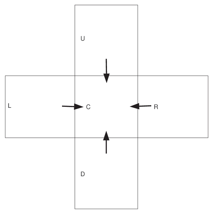
The four spatial weighted averages of ${{\boldsymbol{M}}\!_{n}}(i,j)$ from its left, right, up and down sides are denoted as ${\overline{{\boldsymbol{M}}\!_{n}}(i,j)}_{\rightarrow}$, ${\overline{{\boldsymbol{M}}\!_{n}}(i,j)}_{\leftarrow}$, ${\overline{{\boldsymbol{M}}\!_{n}}(i,j)}_{\downarrow}$ and ${\overline{{\boldsymbol{M}}\!_{n}}(i,j)}_{\uparrow}$. They are expressed as follows:

Rewriting in matrix form, we get

where ${\boldsymbol{T}}\!_{\leftarrow}={\textbf{T}^{\top}_{\rightarrow}}$, ${\boldsymbol{T}}\!_{\uparrow}={\textbf{T}^{\top}_{\downarrow}}$, with

For each abundance ${\boldsymbol{a}}_{n}$, the associated cost function is:

Here, $\omega_{l},\omega_{r},\omega_{u}$ and $\omega_{d}$ control spatial effect ratios of left, right, up and down direction. In particular, $\omega_{l}=\omega_{r}=\omega_{u}=\omega_{d}$ denotes an average allocation of spatial effects. Considering the regularization term $\sum_{n=1}^{N}R_{n}$ for all $N$ abundance maps, the cost function of the spatially-regularized kernel-NMF is:

The update rule of the abundances for this cost function is obtained by locating $a_{nt}$ in ${\boldsymbol{M}}\!_{n}$ using $a_{nt}={\boldsymbol{M}}\!_{n}(i,j)$, with $i=\lceil\frac{t}{b}\rceil$ and $j=t-(i-1)b$. We get $\textstyle{\nabla_{a_{nt}}(\sum_{n=1}^{N}R_{n})}={\nabla_{{\boldsymbol{M}}\!_{n}(i,j)}{R_{n}}}={\boldsymbol{G}}(i,j)$, where

with

By computing ${\nabla_{a_{nt}}{J_{\textrm{spatial}}}}$ with the above expression, we get the additive update rule for $a_{nt}$:

as well as the multiplicative update rule, where we use ${\eta_{nt}}={a_{nt}}/\big({\sum_{m=1}^{N}a_{mt}\kappa({\boldsymbol{e}}_{n},{\boldsymbol{e}}_{m})+{\boldsymbol{G}}(i,j)}\big)$:

References

- [1] P. Comon and C. Jutten, Handbook of Blind Source Separation: Independent Component Analysis and Applications, 1st ed. Academic Press, 2010.
- [2] N. Gillis, “The why and how of nonnegative matrix factorization,” ArXiv e-prints, Jan. 2014.
- [3] D. D. Lee and H. S. Seung, “Learning the parts of objects by non-negative matrix factorization.” Nature, vol. 401, no. 6755, pp. 788–791, Oct. 1999.
- [4] G. Buchsbaum and O. Bloch, “Color categories revealed by non-negative matrix factorization of munsell color spectra.” Vision Research, vol. 42, no. 5, pp. 559–63, 2002.
- [5] D. Guillamet, M. Bressan, and J. Vitria, “A weighted non-negative matrix factorization for local representations,” in Computer Vision and Pattern Recognition, 2001. CVPR 2001. Proceedings of the 2001 IEEE Computer Society Conference on, vol. 1, 2001, pp. I–942–I–947 vol.1.
- [6] S. Z. Li, X. W. Hou, H. J. Zhang, and Q. S. Cheng, “Learning spatially localized, parts-based representation,” in Computer Vision and Pattern Recognition, 2001. CVPR 2001. Proceedings of the 2001 IEEE Computer Society Conference on, vol. 1, 2001, pp. I–207–I–212 vol.1.
- [7] I. Buciu and I. Pitas, “Application of non-negative and local non negative matrix factorization to facial expression recognition,” in 17th International Conference on Pattern Recognition, vol. 1, Cambridge, UK, 2004, pp. 288–291.
- [8] P. Smaragdis, “Non-negative Matrix Factor Deconvolution; Extraction of Multiple Sound Sources from Monophonic Inputs,” in Proceedings of the Fifth International Conference, on Independent Component Analysis and Blind Signal Separation, ICA 2004, Granada, Spain, 22-24 Sep. 2004, pp. 494–499.
- [9] C. Févotte, N. Bertin, and J.-L. Durrieu, “Nonnegative Matrix Factorization with the Itakura-Saito Divergence: With Application to Music Analysis,” Neural Computation, vol. 21, no. 3, pp. 793–830, Sep. 2008.
- [10] W. Liu and N. Zheng, “Non-negative matrix factorization based methods for object recognition,” Pattern Recognition Letters, vol. 25, no. 8, pp. 893–897, 2004.
- [11] S. Wild, J. Curry, and A. Dougherty, “Improving non-negative matrix factorizations through structured initialization,” Pattern Recognition, vol. 37, no. 11, pp. 2217–2232, Nov. 2004.
- [12] K. Devarajan, “Nonnegative Matrix Factorization: An Analytical and Interpretive Tool in Computational Biology,” PLoS Comput Biol, vol. 4, no. 7, Jul. 2008.
- [13] J.-P. Brunet, P. Tamayo, T. R. Golub, and J. P. Mesirov, “Metagenes and molecular pattern discovery using matrix factorization,” Proceedings of the National Academy of Sciences of the United States of America, vol. 101, no. 12, pp. 4164–4169, 2004.
- [14] P. M. Kim and B. Tidor, “Subsystem identification through dimensionality reduction of large-scale gene expression data.” Genome research, vol. 13, no. 7, pp. 1706–1718, 2003.
- [15] S. Young, P. Fogel, and D. Hawkins, “Clustering scotch whiskies using non-negative matrix factorization,” Q&SPES News, vol. 14, pp. 11–13, 2006.
- [16] W. Xu, X. Liu, and Y. Gong, “Document clustering based on non-negative matrix factorization,” in Proceedings of the 26th annual international ACM SIGIR conference on Research and development in informaion retrieval, ser. SIGIR ’03. New York, NY, USA: ACM, 2003, pp. 267–273.
- [17] C. Ding, X. He, and H. D. Simon, “On the equivalence of nonnegative matrix factorization and spectral clustering,” in Proc. SIAM Data Mining Conf, 2005, pp. 606–610.
- [18] T. Li and C. Ding, “The relationships among various nonnegative matrix factorization methods for clustering,” in Proceedings of the Sixth International Conference on Data Mining, ser. ICDM ’06. Washington, DC, USA: IEEE Computer Society, 2006, pp. 362–371.
- [19] A. Cichocki, R. Zdunek, A. H. Phan, and S.-i. Amari, Nonnegative matrix and tensor factorizations: applications to exploratory multi-way data analysis and blind source separation. Wiley Publishing, 2009.
- [20] S. A. Vavasis, “On the complexity of nonnegative matrix factorization,” SIAM Journal on Optimization, vol. 20, no. 3, pp. 1364–1377, Oct. 2009.
- [21] N. Gillis, “Nonnegative matrix factorization: Complexity, algorithms and applications,” Ph.D. dissertation, Université catholique de Louvain, Feb. 2011.
- [22] K. Huang, N. Sidiropoulos, and A. Swami, “Non-negative matrix factorization revisited: Uniqueness and algorithm for symmetric decomposition,” IEEE Transactions on Signal Processing, vol. 62, no. 1, pp. 211–224, Jan. 2014.
- [23] D. Leggett, “Numerical analysis of multicomponent spectra,” Analytical Chemistry, vol. 49, pp. 276—281, 1977.
- [24] P. Paatero and U. Tapper, “Positive matrix factorization: A non-negative factor model with optimal utilization of error estimates of data values,” Environmetrics, vol. 5, no. 2, pp. 111–126, 1994.
- [25] D. D. Lee and H. S. Seung, “Algorithms for Non-negative Matrix Factorization,” in Advances in Neural Information Processing Systems 13. MIT Press, Apr. 2001, pp. 556–562.
- [26] H. Kim and H. Park, “Nonnegative matrix factorization based on alternating nonnegativity constrained least squares and active set method,” SIAM Journal on Matrix Analysis and Applications, vol. 30, no. 2, pp. 713–730, Jul. 2008.
- [27] P. Hoyer and P. Dayan, “Non-negative matrix factorization with sparseness constraints,” Journal of Machine Learning Research, vol. 5, pp. 1457–1469, 2004.
- [28] H. Kim and H. Park, “Sparse non-negative matrix factorizations via alternating non-negativity-constrained least squares for microarray data analysis,” Bioinformatics, vol. 23, no. 12, pp. 1495–1502, Jun. 2007.
- [29] V. P. Pauca, J. Piper, and R. J. Plemmons, “Nonnegative matrix factorization for spectral data analysis,” Linear Algebra and its Applications, vol. 416, no. 1, pp. 29 – 47, 2006.
- [30] S. Jia and Y. Qian, “Constrained nonnegative matrix factorization for hyperspectral unmixing,” IEEE Transactions on Geoscience and Remote Sensing, vol. 47, no. 1, pp. 161–173, Jan. 2009.
- [31] Y. Qian, S. Jia, J. Zhou, and A. Robles-Kelly, “Hyperspectral unmixing via sparsity-constrained nonnegative matrix factorization,” IEEE Transactions on Geoscience and Remote Sensing, vol. 49, no. 11, pp. 4282–4297, Nov. 2011.
- [32] M.-D. Iordache, J. Bioucas-Dias, and A. Plaza, “Total variation spatial regularization for sparse hyperspectral unmixing,” IEEE Transactions on Geoscience and Remote Sensing, vol. 50, no. 11, pp. 4484–4502, Nov. 2012.
- [33] C. Ding, T. Li, W. Peng, and H. Park, “Orthogonal nonnegative matrix t-factorizations for clustering,” in Proceedings of the 12th ACM SIGKDD international conference on Knowledge discovery and data mining, ser. KDD ’06. New York, NY, USA: ACM, 2006, pp. 126–135.
- [34] H. Li, T. Adal, W. Wang, D. Emge, A. Cichocki, and A. Cichocki, “Non-negative matrix factorization with orthogonality constraints and its application to raman spectroscopy,” The Journal of VLSI Signal Processing Systems for Signal, Image, and Video Technology, vol. 48, no. 1-2, pp. 83–97, 2007.
- [35] G. Zhou, S. Xie, Z. Yang, J.-M. Yang, and Z. He, “Minimum-volume-constrained nonnegative matrix factorization: Enhanced ability of learning parts,” IEEE Transactions on Neural Networks, vol. 22, no. 10, pp. 1626–1637, Oct. 2011.
- [36] Y. M. Masalmah and M. Veléz-Reyes, “A full algorithm to compute the constrained positive matrix factorization and its application in unsupervised unmixing of hyperspectral imagery,” in SPIE Defense and Security Symposium. International Society for Optics and Photonics, 2008, pp. 69 661C–69 661C.
- [37] Z. Yang and E. Oja, “Quadratic nonnegative matrix factorization,” Pattern Recognition, vol. 45, no. 4, pp. 1500 – 1510, 2012.
- [38] J. Shawe-Taylor and N. Cristianini, Kernel Methods for Pattern Analysis. Cambridge, UK: Cambridge University Press, 2004.
- [39] V. Vapnik, The Nature of Statistical Learning Theory. New York, NY, USA: Springer-Verlag, 1995.
- [40] B. Schölkopf, A. Smola, and K.-R. Müller, “Nonlinear component analysis as a kernel eigenvalue problem,” Neural computation, vol. 10, no. 5, pp. 1299–1319, Jul. 1998.
- [41] R. Jenssen, “Kernel entropy component analysis,” IEEE Transactions on Pattern Analysis and Machine Intelligence, vol. 32, no. 5, pp. 847–860, 2010.
- [42] D. Zhang, Z. Zhou, and S. Chen, “Non-negative matrix factorization on kernels,” in Lecture Notes in Computer Science, vol. 4099. Springer, 2006, pp. 404–412.
- [43] C. Ding, T. Li, and M. I. Jordan, “Convex and Semi-Nonnegative Matrix Factorizations,” IEEE Transactions on Pattern Analysis and Machine Intelligence, vol. 32, no. 1, pp. 45–55, Nov. 2010.
- [44] Y. Li and A. Ngom, “A new kernel non-negative matrix factorization and its application in microarray data analysis,” in 2012 IEEE Symposium on Computational Intelligence in Bioinformatics and Computational Biology (CIBCB), San Diego, CA, USA, May. 2012, pp. 371–378.
- [45] P. Honeine and C. Richard, “Preimage problem in kernel-based machine learning,” IEEE Signal Processing Magazine, vol. 28, no. 2, pp. 77–88, 2011.
- [46] S. Mika, B. Schölkopf, A. Smola, K.-R. Müller, M. Scholz, and G. Rätsch, “Kernel PCA and de-noising in feature spaces,” in Proc. of the 1998 conference on advances in neural information processing systems II. Cambridge, MA, USA: MIT Press, 1999, pp. 536–542.
- [47] M. Kallas, P. Honeine, C. Richard, C. Francis, and H. Amoud, “Non-negativity constraints on the pre-image for pattern recognition with kernel machines,” Pattern Recognition, vol. 46, no. 11, pp. 3066 – 3080, 2013.
- [48] B. Kanagal and V. Sindhwani, “Rank selection in low-rank matrix approximations: A study of cross-validation for nmfs,” in Low-rank Methods for Large-scale Machine Learning, in NIPS Workshop, Whistler, Canada, December 2010.
- [49] I. Buciu, N. Nikolaidis, and I. Pitas, “Nonnegative matrix factorization in polynomial feature space,” IEEE Transactions on Neural Networks, vol. 19, no. 6, pp. 1090–1100, Jun. 2008.
- [50] P. Comon and C. Jutten, Eds., Handbook of Blind Source Separation: Independent Component Analysis and Applications. Academic Press, Mar. 2010.
- [51] S. An, J.-M. Yun, and S. Choi, “Multiple kernel nonnegative matrix factorization,” in Acoustics, Speech and Signal Processing (ICASSP), 2011 IEEE International Conference on. IEEE, 2011, pp. 1976–1979.
- [52] H. Lee, A. Cichocki, and S. Choi, “Kernel nonnegative matrix factorization for spectral {EEG} feature extraction,” Neurocomputing, vol. 72, no. 13–15, pp. 3182 – 3190, 2009, hybrid Learning Machines (HAIS 2007) / Recent Developments in Natural Computation (ICNC 2007).
- [53] B. Pan, J. Lai, and W. Chen, “Nonlinear nonnegative matrix factorization based on Mercer kernel construction,” Pattern Recognition, vol. 44, no. 10-11, pp. 2800 – 2810, 2011.
- [54] M. Kallas, P. Honeine, C. Richard, C. Francis, and H. Amoud, “Non-negative pre-image in machine learning for pattern recognition,” in 19th European Signal Processing Conference, Barcelona, Spain, 29 Aug. - 2 Sep. 2011.
- [55] H. Lantéri, C. Theys, C. Richard, and D. Mary, “Regularized split gradient method for nonnegative matrix factorization,” in 2011 IEEE International Conference on Acoustics, Speech and Signal Processing (ICASSP), 2011, pp. 1133–1136.
- [56] J. Piper, V. P. Pauca, R. J. Plemmons, and M. Giffin, “Object characterization from spectral data using nonnegative factorization and information theory,” in Proceedings of AMOS Technical Conference, 2004.
- [57] T. Virtanen, “Sound source separation using sparse coding with temporal continuity objective,” vol. 3, 2003, pp. 231–234.
- [58] Z. Chen and A. Cichocki, “Nonnegative matrix factorization with temporal smoothness and/or spatial decorrelation constraints,” in Laboratory for Advanced Brain Signal Processing, RIKEN, Tech. Rep, 2005.
- [59] A. Halimi, Y. Altmann, N. Dobigeon, and J. Tourneret, “Nonlinear unmixing of hyperspectral images using a generalized bilinear model,” IEEE Transactions on Geoscience and Remote Sensing, vol. 49, no. 11, pp. 4153–4162, Nov. 2011.
- [60] R. Clark, G. Swayze, and A. Gallagher, “Mapping minerals with imaging spectroscopy,” US Geological Survey, Office of Mineral Resources Bulletin, vol. 2039, pp. 141–150, 1993.
- [61] N. Dobigeon, J.-Y. Tourneret, and C.-I. Chang, “Semi-supervised linear spectral unmixing using a hierarchical bayesian model for hyperspectral imagery,” IEEE Transactions on Signal Processing, vol. 56, no. 7, pp. 2684–2695, Jul. 2008.
- [62] M. Winter, “N-FINDR: an algorithm for fast autonomous spectral end-member determination in hyperspectral data: an algorithm for fast autonomous spectral end-member determination in hyperspectral data,” Proc. of SPIE: Imaging Spectrometry V, vol. 3753, no. 10, 1999.
- [63] J. Nascimento and J. Bioucas Dias, “Vertex component analysis: a fast algorithm to unmix hyperspectral data,” IEEE Transactions on Geoscience and Remote Sensing, vol. 43, no. 4, pp. 898–910, Apr. 2005.
- [64] D. Heinz and C. Chang, “Fully constrained least squares linear spectral mixture analysis method for material quantification in hyperspectral imagery,” IEEE Transactions on Geoscience and Remote Sensing, vol. 39, no. 3, pp. 529–545, Mar. 2001.
- [65] J. Chen, C. Richard, and P. Honeine, “Nonlinear unmixing of hyperspectral data based on a linear-mixture/nonlinear-fluctuation model,” IEEE Transactions on Signal Processing, vol. 61, no. 2, pp. 480–492, Jan. 2013.
- [66] N. Yokoya, J. Chanussot, and A. Iwasaki, “Nonlinear unmixing of hyperspectral data using semi-nonnegative matrix factorization,” IEEE Transactions on Geoscience and Remote Sensing, vol. 52, no. 2, pp. 1430–1437, Feb. 2014.
- [67] A. Huck, M. Guillaume, and J. Blanc-Talon, “Minimum dispersion constrained nonnegative matrix factorization to unmix hyperspectral data,” IEEE Transactions on Geoscience and Remote Sensing, vol. 48, no. 6, pp. 2590–2602, Jun. 2010.
- [68] C.-J. Lin, “On the convergence of multiplicative update algorithms for nonnegative matrix factorization,” Neural Networks, IEEE Transactions on, vol. 18, no. 6, pp. 1589–1596, Nov 2007.
- [69] Z. Yang and E. Oja, “Linear and nonlinear projective nonnegative matrix factorization,” Neural Networks, IEEE Transactions on, vol. 21, no. 5, pp. 734–749, May 2010.