Coronal Mass Ejections from
the Sun - Propagation and
Near Earth Effects.
A thesis
Submitted in partial fulfillment of the requirements
Of the degree of
Doctor of Philosophy
By
Arun Babu K. P.
20083021
![[Uncaptioned image]](1407.4258v1/logo.png)
INDIAN INSTITUTE OF SCIENCE EDUCATION AND RESEARCH PUNE
July, 2014
Certificate
Certified that the work incorporated in the thesis entitled
“Coronal Mass Ejections from the Sun - Propagation and Near Earth Effects”,
submitted by Arun Babu K. P. was carried out by the candidate, under my supervision. The work presented here or any part of it has not been included in any other thesis submitted previously for the award of any degree or diploma from any other University or institution.
Date Dr. Prasad Subramanian
Declaration
I declare that this written submission represents my ideas in my own words and where others’ ideas have been included, I have adequately cited and referenced the original sources. I also declare that I have adhered to all principles of academic honesty and integrity and have not misrepresented or fabricated or falsified any idea/data/fact/source in my submission. I understand that violation of the above will be cause for disciplinary action by the Institute and can also evoke penal action from the sources which have thus not been properly cited or from whom proper permission has not been taken when needed.
Date Arun Babu K. P.
Roll No.- 20083021
To
my
Mom & Dad
Acknowledgements
This thesis is the fruit of my long journey in obtaining my PhD. I was not left alone in this journey, but was with support and encouragement of numerous people including, my well wishers, my friends, colleagues and collaborators. It is a pleasant task to express my thanks to all those who contributed in many ways to the success of this study and made it an unforgettable experience for me.
It is my great pleasure to express my gratitude to my supervisor Dr. Prasad Subramanian for his guidance, support and encouragement in pursuing this work. To be honest I was extremely impressed by his personality and his encouraging nature during my PhD interviews and the introductory talk about the research fields given by the faculties to the PhD students. There was no need of any second thought for me to join him to pursue my PhD. He was very friendly to us and was known as the ‘coolest guide’ in IISER among my fellow students.
I would like to thank Dr. K. N. Ganesh, Director, IISER-Pune, for the excellent research facilities and academic environment here. I acknowledge the financial support from IISER-Pune in the form of research fellowship. Many thanks to IISER administration, library, computer, transport and house-keeping staff.
I acknowledge the RESPOND and CAWSES II programs administered by Indian Space Research Organisation (ISRO) for their financial support during my PhD. I acknowledge Asian Office of Aerospace Research and Development (AOARD) for the financial support during the final year of my PhD.
It was an honour for me to work with the GRAPES-3 team (TIFR, Mumbai). I thank GRAPES-3 team for providing the data, which I used to study the Forbush decreases, that cover major part of my thesis. I specially thank Prof. H. M. Antia (TIFR, Mumbai) and Prof. Sunil Gupta (TIFR, Mumbai) for their help and discussions. Prof. H. M. Antia helped me in analysing the GRAPES-3 data, he was always available and never let me wait for more than five minutes for his help, discussion and suggestions via emails. Prof. Sunil Gupta, who was also one of my research advisory committee members helped me understand the basics of the ‘GRAPES-3 muon telescope’, his discussions and advises have benefited me greatly during my PhD. I thank P. K. Mohanty and Atul Jain (TIFR, Mumbai) for familiarizing me with the GRAPES-3 and I thank all other members of GRAPES-3 collaboration. It is a pleasure to thank Dr. Apratim Chatterji who was in my research advisory committee for his valuable feedback and suggestions. I am happy to express my gratitude to Prof. Alejandro Lara Sánchez (UNAM, Mexico) for his useful discussions.
It is really a nice experience to be in the solar physics group of IISER with Mayur, Nishtha and Tomin. I enjoyed working with Adwiteey, Bhavesh, Ajay and Abhishikth. I have enjoyed our solar physics journal club meetings. I thank Dr. Durgesh Tripati (IUCAA, Pune) for his initiation to start our journal club. It was really nice time with you all, Prasad, Divya, Durgesh, Mayur, Nishtha, Rohit, Ajay, Tomin, Srividya, Sargam and Girjesh.
It was fun and refreshing being with the fellow students. I thank Arthur, Murthy, Mayur, Kajari, Abishek, Resmi, Kanika, Padma, Somu, Ramya, Madhan, Neeraj, Shweta, Mahendra, Mandar, Vimal, Aditya, Nishtha, Shishir, Sanku, Rohit, Harshini, Kunal and Nitin. The days in common room were very cherishing with Ludo games, ice-cream parties, birthday celebrations and assignment writing. Hostel life in IISER was also so enjoyable with many hostel shiftings. It was really nice to have Arthur as my room partner, who took care of me as my brother and provided tasty food for me in our kitchen. The entertainment section was mainly managed by Mayur, who provide us movies with his passion of downloading. Kajari is a good buddy and shares my interests in photography and in food. She is always ready for any adventure. The heated unending philosophical discussions were provided by Abhishek in the company of Resmi, Kajari and Mayur. I thank Lal, Sandeep, Kajari and Anusha for their company and the bike rides we had together. The life in IISER was not without few down and depressed moments. I thank Prasad, Arthur, Kajari, Mayur and Resmi for the comfort and assurances they gave me.
I thank Aaron, Abner and Adrin of ‘FOUR ACES’, my long-time friends for their support and encouragement. Conversations with you were always cheerful and motivating.
At last and the most I thank my family, who support me always. I thank my mother, father and brother for their love, support and encouragement throughout my life.
Arun Babu K. P.
Abstract
Owing to our dependance on spaceborne technology, an awareness of disturbances in the near-Earth space environment is proving to be increasingly crucial. Earth-directed Coronal mass ejections (CMEs) emanating from the Sun are the primary drivers of space weather disturbances. Studies of CMEs, their kinematics, and their near-Earth effects are therefore gaining in importance.
The effect of CMEs near the Earth is often manifested as transient decreases in galactic cosmic ray intensity, which are called Forbush decreases (FDs). In this thesis we probe the structure of CMEs and their associated shocks using FD observations by the GRAPES-3 muon telescope at Ooty. We have established that the cumulative diffusion of galactic cosmic rays into the CME is the dominant mechanism for causing FDs (Chapter 3).
This diffusion takes place through a turbulent sheath region between the CME and the shock. One of our main results concerns the turbulence level in this region. We have quantitatively established that cross-field diffusion aided by magnetic field turbulence accounts for the observed lag between the FD and the magnetic field enhancement of the sheath region (Chapter 4).
We have also investigated the nature of the driving forces acting on CMEs in this thesis. Using CME data from the SECCHI coronagraphs aboard STEREO sapcecraft, we have found evidence for the non-force-free nature of the magnetic field configuration inside these CMEs, which is the basis for the (often-invoked) Lorentz self-force driving (Chapter 5).
Taken together the work presented in this thesis is a comprehensive attempt to characterise CME propagation from typical coronagraph fields of view to the Earth.
Publications
The research work presented in this thesis has appeared in the following publications.
Publications in international refereed journals
- 1.
“High-rigidity Forbush decreases: due to CMEs or Shock?”, K. P. Arunbabu et al., 2013, Astronomy & Astrophysics, 555, 139
- 2.
“Self-similar expansion of solar coronal mass ejections: implications for Lorentz self-force driving”, P. Subramanian, K. P. Arunbabu, A. Vourlidas, A. Mauriya, 2014, The Astrophysical Journal, 790, 125
- 3.
“Relation of Forbush decreases with the Interplanetary magnetic field enhancements ”, K. P. Arunbabu et al. in preparation
Refereed conference proceedings
- 1.
“How are Forbush decreases related with IP magnetic field enhancements ?”, K. P. Arunbabu et al., Proceedings of the International Symposium on Solar Terrestrial Physics, ASI Conference Series, 2013, 10, 95.
Presentations in symposia/conferences
- 1.
Meeting of the Astronomical Society of India, 2014 March 20-22 , IISER Mohali, “How are Forbush decreases related with IP magnetic field enhancements ?”, K. P. Arun Babu, Prasad Subramanian, Sunil Gupta, H. M. Antia, (oral presentation)
- 2.
International Symposium on Solar Terrestrial Physics, 2012 November 6-9 , IISER Pune, “How are Forbush decreases related with IP magnetic field enhancements ?”, K. P. Arun Babu, Prasad Subramanian, Sunil Gupta, H. M. Antia, (poster presentation)
- 3.
39th COSPAR Scientific Assembly, 14 - 22 July 2012,Mysore, India, “Forbush decrease observed in GRAPES-3”, K. P. Arun Babu, Prasad Subramanian, Sunil Gupta, H. M. Antia, GRAPES-3 team, (poster presentation)
- 4.
Workshop on ’Physics of the Solar Transition Region and Corona’ , IUCAA Pune, 2011 September 5-7 , “Coronal Mass Ejections & Forbush Decrease”, K. P. Arun Babu (oral presentation)
- 5.
Asia Oceanic Geoscience Society International conference AOGS 2010 July 5-9, Hyderabad, “ Forbush decreases observed with GRAPES-3”, K. P. Arun Babu, Prasad Subramanian, Sunil Gupta, H. M. Antia, (oral presentation)
- 6.
Workshop and Winter School on AstroParticle Physics (WAPP 2009), 2009 December 10-12, Bose Institute, Darjeeling, “Forbush decreases observed in GRAPES-3”, K. P. Arun Babu, Prasad Subramanian, (oral presentation).
Chapter 1 Introduction
In this chapter we will introduce the fundamental physics and concepts that are discussed in this thesis, beginning with a short introduction to the Sun, its interior, various layers, atmosphere, and activity. This is followed by an introduction to coronal mass ejections (CMEs) comprising a historical account of CME observations, physical properties, initiation models, and propagation models. This is followed by an introduction to the Sun-Earth connections and the effects of the solar wind and CMEs on near-Earth space weather
1.1 Sun
The Sun, our nearest star and the center of our solar system, is a main sequence star of spectral type G2V. The Sun has a total luminosity , mass and radius (Foukal, 2004). The Sun was born from a giant molecular cloud of approximate mass M which began to gravitationally collapse and fragment. The process of collapse and fragmentation continued until one of these fragments attained a central temperature large enough to start hydrogen fusion, about years ago (Prialnik, 2009). At this point the energy produced by the hydrogen fusion was high enough to counterbalance the gravitational collapse. Currently, the Sun is in a stable configuration, on the Main Sequence, where it is in hydrostatic equilibrium . The Sun will continue to maintain this stable state for about another years before entering the red giant phase. At this point the Sun will expand to about 100 times its current size and begin shedding its outer layers, due to successive nuclear burning in ever more distant shells. This will ultimately leads to the total loss of the outer envelope exposing a degenerate core, in which all nuclear burning has ceased, called a white dwarf (Phillips, 1995).
1.1.1 Solar Interior

The entire energy emitted by the Sun is produced by ‘hydrogen fusion’ reactions. The core is the central part of the Sun where the temperature and pressure are high enough for the fusion reaction to occur. The temperatures in the core are around and the pressure exceeds atmospheres. The core extends up to . Outside of the core is the radiative zone (), where thermal radiation is the most efficient means of transporting the intense energy generated in the core (in the form of high energy photons) outward. The temperature drops from about at the bottom of the radiative zone to just below the convection zone. Due to the high densities ( ) in the radiative zone the mean free path of the photons is very small (); hence it can take tens to hundreds of thousands of years for photons to escape. The radiative zone and the convection zone are separated by a transition layer, the tachocline. The convection zone is the outer layer of the Sun (). The temperature of the convection zone is lower than that in the radiative zone and heavier atoms are not fully ionized. As a result, radiative heat transport is less effective. The density of the gases in this zone are low enough to have convective currents. Material heated at the tachocline pick up heat and expand. This reduces the density of material and allows it to rise. Thermal convection carry the majority of the heat outward to the Sun’s photosphere. The material cools off at the photosphere, which increases its density and causes it to sink to the base of the convection zone. At the convection zone it picks up more heat from the top of the radiative zone and the cycle continues. The visible surface of the Sun, the photosphere, is the layer below which the Sun becomes opaque to visible light. Above the photosphere visible sunlight is free to propagate into space, and its energy escapes the Sun entirely.

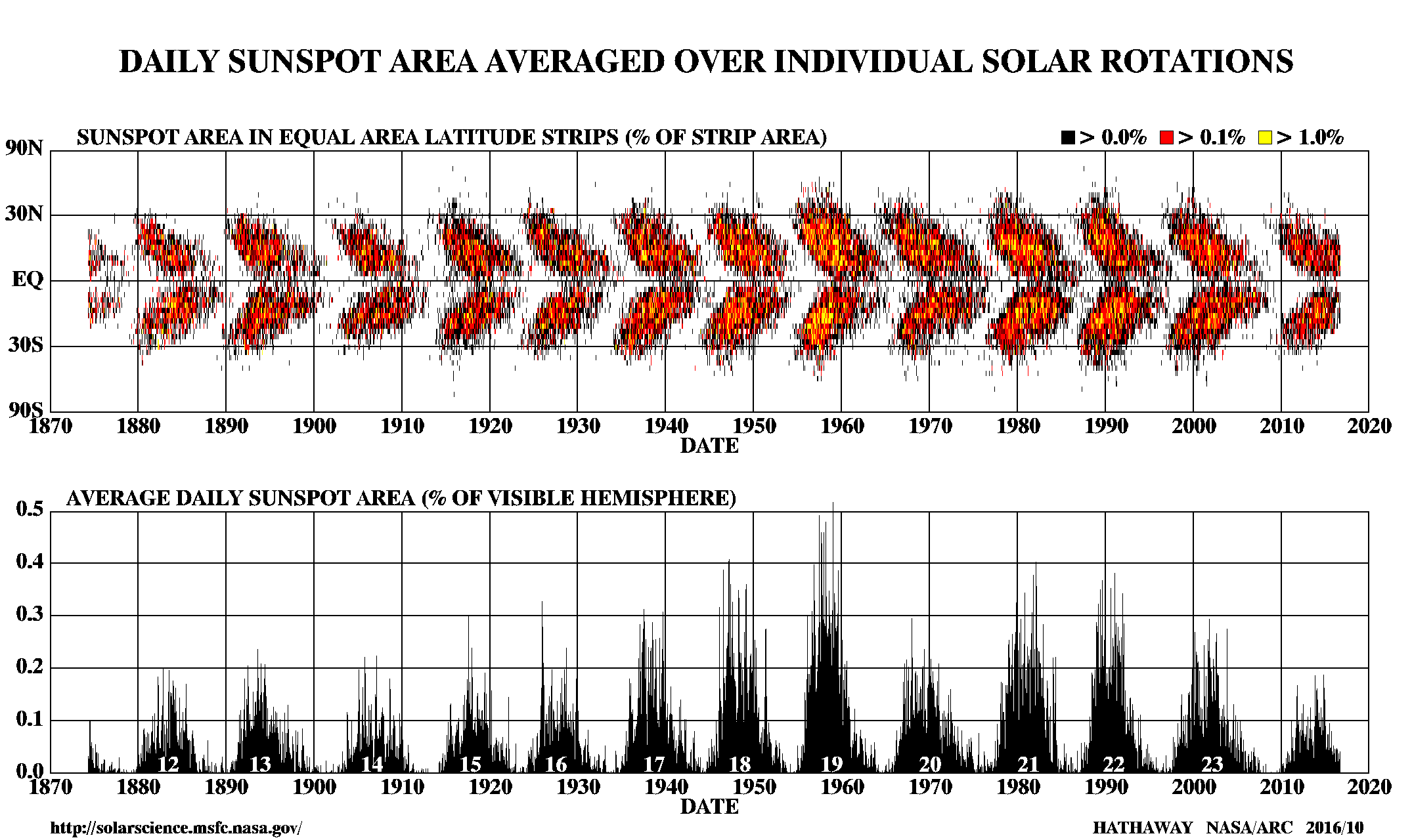
The core and the radiative zones of the Sun rotate rigidly (as a solid body), where as the convection zone rotates differentially. There is a thin interface between these two regions known as the tachocline. This region is subjected to large shear flows due to the meeting of the two bodies rotating at different rates. These flows are believed to be the mechanism which generates the Sun’s large-scale magnetic field and powers the solar dynamo. The Sun’s magnetic field is mainly dipolar and aligned to the rotation axis. Each hemisphere has an opposite dominant polarity (see the left panel in Figure 1.2). The differential rotation of the convection zone winds up this field (see the middle panel in Figure 1.2). This large scale twisting transforms poloidal field to toroidal field which is known as the -effect. As the field is twisted up the magnetic pressure increases and bundles of magnetic field lines (flux ropes) can become unstable and rise up in the from of loops. Due to solar rotation, the Coriolis effect twists these loop back towards north-south orientation, reinforcing the original poloidal field. This is known as the -effect (see the right panel in Figure 1.2) and completes the -dynamo. When magnetic loops become buoyant and rise up through the surface they are visible as sunspots on-disk and mark the footprints of large loops which extend into the solar atmosphere. In a given hemisphere the leading sunspot and trailing sunspot will have opposite polarities, this order is reversed in the other hemisphere (Hale’s Law). The tilt angle of the sunspots pairs have a mean value of relative to the solar equator (Joy’s Law). Sunspots are known to migrate from high latitudes towards the equator over an 11 year cycle (Sporer’s Law; see figure 1.3). The net affect is an increase in opposite polarity field at the poles, ultimately the majority of the field will be oppositely oriented and the dipole will flip. This occurs every 11 years, thus a complete cycle takes 22 years (N to S to N). The activity of the Sun, in the form of active regions, flares, transient events, and other associated phenomenon, is modulated by this cycle (see figure 1.3 lower).

1.1.2 Solar Atmosphere
The photosphere is the layer beyond which the optical depth falls below unity. The Sun’s atmosphere typically refers to all the regions above the photosphere. Based on their density, temperature, and composition the solar atmosphere is usually separated into three regions, the photosphere, chromosphere and corona as shown in Figure 1.4. However, the separation solar atmosphere is a simplification as the atmosphere is an inhomogeneous mix of different plasma properties due to up-flows, down-flows, heating, cooling and other dynamic processes. The density of the plasma generally decreases with increasing height through these regions. The temperature decreases in photosphere, reaching a minimum in the chromosphere, then slowly rises until there is a rapid increase at the transition region which continues into the corona. This rapid increase in temperature embodies the so-called ‘coronal heating problem’.

An important parameter in describing the solar atmosphere is the plasma- term, the ratio of the thermal to magnetic pressures:
| (1.1) |
where is the number density and the permeability of free space. In the photosphere the plasma- is large (Figure 1.5). The plasma- decreases farther up in the solar atmosphere, before increasing again in the outer corona.

Photosphere
The photosphere is the lowest of the three layers of solar atmosphere. It is the visible surface of the Sun and is defined as the height where the optical depth, at visible wavelengths, equals 2/3 ( ). This is the mean optical depth at which the photospheric radiation is emitted. The effective temperature () and blackbody temperature of the photosphere matches here. This can be seen by substituting and (F is the total radiative flux) in the general solution of the radiative transfer equation:
| (1.2) |
which gives,
| (1.3) |
implying that (Foukal, 2004). The temperature drops from at the base of the photosphere to 4,400K at the top. The spectrum of photospheric radiation is that of a blackbody with a large number of absorption features, Fraunhofer lines, due the upper layers of the atmosphere superimposed on it. The number density of photosphere ranges from over the depth of the photosphere ().
One of the main observable features in the photosphere is granulation. This represents convection currents operating just below the photosphere, which transport heat from below to the surface. Granules are small-scale features made up of brighter regions isolated by darker lanes, interpreted as the upflow of hot material to the surface which then flows horizontally and cools, flowing back down in the dark lanes. Typical granules are of the order of in diameter. They have lifetimes of 5-10 minutes with vertical flow velocities of hundreds to thousands . There are also larger scale flow patterns known as mesogranulation and supergranulation. Mesogranules are typically in diameter, and have lifetimes of hours with vertical flows of the order of tens of . Supergranules are larger still at diameters of , and consequently have longer lifetimes of days. Supergranules have large horizontal flows and smaller vertical flows of the order of . Sunspots appear in the photosphere as darker regions due to their lower temperature (). They appear dark since convection is suppressed by the strong kilogauss magnetic fields. Sunspots play an important role in the activity of the Sun as they are the source of solar flares and many CMEs.
Chromosphere
The chromosphere is the middle layer of solar atmosphere, which lies above the photosphere. At this layer the temperature initially decreases to a minimum of before increasing to with increasing height. It occupies a region approximately thick with a density of about . The chromosphere has a split structure between the hot bright magnetic network and the cooler darker internetwork (Gallagher et al., 1999). Spicules, which are jets of plasma are also observed on the limb. These jet-like structures have diameters of hundreds of kilometres, attaining heights of tens of thousands of kilometres above the solar surface, with flows of the order of lasting 5 - 10 minutes.
The nature of the heating mechanism of chromosphere is unclear. Observations imply that there must be some form of energy deposition occurring. Neither radiation nor conduction can be the source as the temperature is lower at the base of the lower chromosphere and photosphere than in chromosphere proper (and would thus violate the laws of thermodynamics). Since the chromosphere is in hydrostatic equilibrium, mass motions are neither observed nor applicable. The most likely source of the energy (heat flux) is the dissipation of compressional or sound waves Schwarzschild (1948). The convective plasma motions of the photosphere launches sound waves into the chromosphere. These sound waves travel upwards with little dissipation. As the density drops, the waves steepen and form shocks which rapidly dissipate energy, thereby heating the chromosphere. This type of acoustic heating is not appropriate in the network regions. In these regions the strong magnetic fields suppress the convective motions which drive the waves. This led to the idea of Aflvén wave heating which is first introduced by Osterbrock (1961). Aflvén waves are magneto-hydrodynamic waves which propagate along magnetic fields. The restoring force is provided by magnetic tension and the ion mass provides the inertia. Here the magnetic field itself is responsible for transportation and deposition of the energy from the photospheric motions. This type of heating matches well with observations of plage and emerging flux regions. Both of these show strong heating which imply that the heat flux is related to the magnetic field strength.
Filaments are often seen over active regions as dark channels in on-disk observations or as prominences when observed on the limb as bright features. The transition region lies between the chromosphere and corona, here the temperature rapidly jumps (over 100 km) to above 1 MK. Above the transition region the magnetic field dominates and determines the structures.
Corona
The tenuous, hot, outer layer of the solar atmosphere is known as the corona. The electron density of the solar corona ranges from at its base, above the photosphere, to for heights (Aschwanden, 2006). The density varies depending on the feature, such as the open magnetic structures of coronal holes can have densities in the region of , streamers have densities in the region of while active regions have densities in the region of . The temperature in the corona is generally above but again varies across different coronal features. Coronal holes have the lowest temperature (less than ) followed by quiet Sun regions at . Active regions are the hottest at with flaring loops reaching even higher temperatures. The high temperatures reached in the corona give rise to EUV and X-ray emission, which have highly ionised iron lines as a prominent feature. The visible corona during eclipses is due to Thomson scattering of photospheric light from free electrons in the coronal plasma. The corona has a number of components:
- •
K-corona (kontinuierliches spektrum) is composed of Thomson-scattered photospheric radiation and dominates below . As a result of the Thomson scattering mechanism, the scattered light is strongly polarised parallel to the solar limb. The high temperatures mean the electrons have high thermal velocities. This will wash out (due to thermal broadening) the Fraunhofer lines, producing a white-light continuum. The intensity of the K-corona is proportional to the density summed along the line-of-sight.
- •
F-corona (Fraunhofer) is composed of Rayleigh-scattered photospheric radiation by dust particles, and dominates above . It forms a continuous spectrum with the superimposed Fraunhofer absorption lines. The radiation has a very low degree of polarisation. The F-corona is also know as Zodiacal light, it can be seen with the naked eye at dawn or dusk under favourable conditions.
- •
E-corona (Emission) is composed of line emission from visible to EUV due to various atoms and ions in the corona. It contain many forbidden line transitions, thus it contains many polarisation states. Some of the strongest lines are Fe xiv 530.3 nm (green-line; visible), H- at 656.3 nm (visible), and Lyman- 121.6 nm (UV).
- •
T-corona (Thermal) is composed of thermal radiation from heated dust particles. It is a continuous spectrum according to the temperature and colour of the dust particles.
1.2 Coronal mass Ejections (CMEs)
Every main sequence star loses mass via dynamic phenomena in its atmosphere that accelerate plasma or particles beyond the escape speed. In the case of our Sun, the outer plasma atmosphere, known as the corona, extends to millions of kilometres. There are two forms of mass loss in Sun: the steady solar wind flow and episodic coronal mass ejections (CMEs). CMEs are large scale eruptions of plasma and magnetic filed which propagate from the Sun into the Heliosphere. Post-eruption, CMEs are driven by the release of energy carried by the magnetic fields advected by the CME (Vourlidas et al., 2000; Subramanian & Vourlidas, 2007). The more energetic CMEs are associated with flares. The solar wind outflows amount to in coronal holes, and in active regions. The CME occurence rate is highly solar cycle dependent. This occurs with an average frequency of few events per day, carrying the mass in the range of , which corresponds to an average mass loss of , which is of solar wind mass loss in coronal holes, or of that in active regions. Further details regarding CME occurrence rate are mentioned below in section § 1.2.2
A typical CME has a mass of (Vourlidas et al., 2002) and a velocity between some times reaching up to close to the Sun (Yashiro et al., 2004). At 1 AU, CME velocities () tend to equilibrate to the solar wind speed (Gopalswamy, 2006; Lindsay et al., 1999). The energies associated with CMEs are of the order of , making them among comparable to flares, the most energetic events on the Sun (Vourlidas et al., 2002).
In this section we give only a brief introduction to CMEs, more detailed reviews can be found in Webb & Howard (2012) and Chen (2011).
1.2.1 Observations of CMEs
Observations of the corona and CMEs are possible only when the photosphere of the visible Sun is occulted. Such occultation occurs naturally during solar eclipses and is artificially created by spaceborne coronagraphs. A coronagraph produces an artificial solar eclipse. It uses an occulting disk to block the Sun’s bright surface, revealing the faint solar corona, stars, planets and sungrazing comets. Coronagraphs view the outward flow of density structures emanating from the Sun by observing photons emitted from photosphere Thomson-scattered by free electrons in solar corona.
The earliest observation of a CME probably dates back to the total solar eclipse of 18 July 1860 in a drawing recorded by Gugliemo Temple shown in figure 1.6 (Eddy, 1974). It took more than 100 years after that for the CME to be formally discovered. The first definitive observation being made on 14 December 1971 by Tousey (1973) using the coronagraph on-board the seventh Orbiting Solar Observatory (OSO-7).
Space-based coronagraphs
A number of orbital coronagraphs were flown in space which provided better data and longer periods of CME observations. Spaceborne coronagraphs which observed CMEs include OSO-7 coronagraph in the early 1970s (Tousey, 1973), Skylab (1973 - 1974; MacQueen et al., 1980), P78-1 (Solwind) (1979 - 1985; Sheelay et al., 1980), and Solar Maximum Mission (SMM) (1980; 1984 - 1989; Hundhausen, 1999). In late 1995, the Solar and Heliospheric observatory (SOHO) was launched. The SOHO spacecraft carries a set of three Large Angle and Spectrometric Coronagraph (LASCO) coronagraphs with nested field of view which image the Sun from (Brueckner et al., 1995). Of the three coronagraphs, the first one, C1 was an internally occulted coronagraph designed to image the innermost corona from in emission lines. C1 ceased operation in June 1998. The other two (C2 and C3) are externally occulted and designed to image the outer corona. The field of view of C2 and C3 are and respectively. Two of the three LASCO coronagraphs (C2,C3) are still operating. In October 2006 two sets of identical coronagraph packages called, the Sun Earth Connection Coronal Heliospheric Investigations (SECCHI) were flown on two spacecrafts called Solar TErrestrial RElations Observatory (STEREO) A and B. The SECCHI package consists of coronagraphs having unprecedented field of view ranging from (COR1), (COR2), (HI1) and (HI2) in white light. These coronagraphs are designed to provide 3-D view of CMEs in the inner and outer corona.
Ground-based coronagraphs
Ground-based instruments for imaging corona are complementary to the space-based ones because they can achieve a better temporal resolution and are not limited by the telemetry rate. However, they are limited by the intensity and temporal variability of the sky. The main operating ground based coronagraphs today include the Mauna Loa Solar Observatory (MLSO) K-coronameter () (Fisher et al., 1981; Koomen et al., 1974) and the green line coronagraphs at Sacramento Peak, New Mexico (Demastus et al., 1973) and Norikura, Japan (Hirayama & Nakagomi, 1974).

1.2.2 Physical properties of CMEs
CME observations have not only led to studies of their morphological properties, but also to statistical analyses of their physical and kinematical properties.
Morphology

A classical picture of a CME observed in white light comprises a three part structure (figure 1.7). It displays a bright leading edge which contains the material swept by the CME. The leading edge is followed by a darker cavity which is due to its low density but has a high magnetic field. The cavity is followed by a bright knot or core, which corresponds to the erupting filament (House et al., 1981). CMEs may also exhibit more complex structures (Pick et al., 2006). In fact less than of CME events possess all the three parts (Webb & Hundhausen, 1987). CMEs come in many different shapes, and much of the variety is believed simply due to the projection effects (Schwenn, 2006). Fundamental difference can be found between narrow CMEs and normal CMEs. The narrow CMEs show jet-like motions probably along open magnetic field, on the other hand normal CMEs are characterized by a closed frontal loop. There are also CMEs without a bright core. Some are due to the fact that the filament material drained down to the solar surface along the stretched magnetic field, some due to the fact that thermal instability had not started to form a filament in the pre-eruption structure, and others might not be related to filament or filament-supporting structure at all.
Angular width
The angular width of CMEs projected in the plane of the sky ranges from (Yashiro et al., 2004), with a significant fraction in the low end (e.g., ) and a small fraction in the high end (e.g., ). CMEs with angular widths less than can be called narrow CMEs (Wang et al., 1998), and others are sometimes called normal CMEs (Yashiro et al., 2004, see Figure 1.8). The average width of LASCO/SOHO CMEs is found to be for limb CMEs. The average width is relatively smaller () during solar activity minimum compared to that during solar maximum () (Yashiro et al., 2004). Halo CMEs , with an apparent angular width of or close to , are simply due to the fact that the CMEs (probably with an angular width of tens of degrees) propagate near the Sun-Earth line, either toward or away from the Earth.

Frequency of occurence
During solar cycle 23, LASCO observations provided unprecedented observations of CMEs . The occurrence rate of CMEs was found to largely track the solar activity cycle, but with a delay of 6- 12 months (Raychaudhuri, 2005; Robbrecht et al., 2009) between the solar cycle maximum and maximum occurence rate of CMEs. Before the launch of SOHO, the average occurrence rate was found to increase from 0.2 per day at solar minimum to 3.5 per day at solar maximum (Webb & Howard, 1994). With the increased sensitivity and wider field of view, the SOHO/LASCO coronagraphs detected CMEs more frequently. The CDAW catalog 11 1 lists around 13,000 CMEs identified visually. The results from this catalog suggest that the CME occurence rate increases from per day near solar minimum to near solar maximum (Gopalswamy et al., 2003; Yashiro et al., 2004). However, the automated software, CACTus3, identified many more events for the same period, with the occurrence rate increasing from per day near solar minimum to per day near solar maximum (Robbrecht et al., 2009). The CME daily occurrence rate detected by the two methods, along with the sunspot number are shown in figure 1.9 for the comparison.

CME speeds
Estimates of the apparent speeds of the leading edges of CMEs range from about . The annual average speeds of Solwind and SMM CMEs varied over the solar cycle from about . Even though their relationship to sunspot number was unclear (Howard et al., 1986; Hundhausen, 1994). On the other hand LASCO CME speeds did generally track sunspot number in Solar Cycle 23 (Yashiro et al., 2004; Gopalswamy, 2010), from . For a typical CMEs, above a height of about the speeds are relatively constant in the field of view of coronagraphs. The slowest CMEs tend to show acceleration while the fastest tend to decelerate (St Cyr et al., 2000; Yashiro et al., 2004; Gopalswamy et al., 2006). This can be expected, considering that CMEs must push through the surrounding solar wind, believed to have a speed of around in the outer corona.
CMEs typically accelerate fast low in the corona until gravity and other drag forces slow them further out. This process continues into the interplanetary medium. The early acceleration for most CMEs occurs low in the solar corona (). Only 17% of all LASCO CMEs experience acceleration out to (St Cyr et al., 2000). Zhang et al. (2001); Zhang et al. (2004) used the observations of flare-associated CMEs close to the limb in the LASCO C1 field of view () and found a three-phase kinematic profile. The first phase is a slow rise () over tens of minutes. The second phase shows rapid acceleration of in the height range during the flare rise phase, and a final phase exhibits propagation at a constant or declining speed. Gallagher, Lawrence & Dennis (2003) and others have identified the strong acceleration region of impulsive CMEs to . The studies of Sheeley et al. (1999) and Srivastava et al. (1999) using LASCO data found that gradually accelerating CMEs looked balloon-like in coronagraph images, but fast CMEs moved at constant speed even as far out as . Sheeley et al. (1999) found that when viewed well out of the sky plane, gradual CMEs looked like smooth halos which accelerated to a limiting value then faded, while fast CMEs had ragged structure and decelerate. In the LASCO field of view slow CMEs tend to accelerate and fast CMEs decelerate, while those around the solar wind speed having constant speeds (Yashiro et al., 2004).
The aerodynamic drag experienced by CMEs while they travel through the interplanetary medium between the Sun and Earth is generally thought to arise due to the coupling of the CMEs to the ambient solar wind. The solar wind strongly mediates CME propagation (Gopalswamy et al., 2000; Manoharan, 2006) in the interplanetary medium, CMEs which start out slow (with respect to the solar wind speed) near the Sun seem to accelerate en route to the Earth, while fast CMEs are decelerated. This fact has been invoked in several studies that derive a heuristic aerodynamic drag coefficient for CMEs to investigate CME slowdown using a simple 1D hydrodynamical model that lends itself to analytical solutions (Borgazzi et al., 2009; Cargill, 2004; Byrne et al., 2010; Maloney & Gallagher, 2010; Vršnak et al., 2010; Vršnak et al., 2013). Subramanian, Lara & Borgazzi (2012) used the viscous drag by the solar wind on the CME to study the velocity of CME in the interplanetary medium.
CME mass & energy estimates
Masses of CMEs are derived from the white light images obtained by coronagraphs. The mass estimates are based on the fact that the white light emission from the corona is mainly due to Thomson scattering of photospheric light by the electrons in the corona. This therefore requires estimation of the coronal density from a series of time-lapse images of a CME by the coronagraph. This involves measurement of electron density, which is computed from the excess brightness after removing the pre-CME brightness. The method is based on the assumption that a single electron at a certain point in the atmosphere will scatter a known amount of solar disk intensity. Thus by measuring the intensity and assuming that all of the mass is in a single volume element, the number of electrons can be computed. The CME mass can be estimated assuming charge neutrality.
Masses and energy calculations of CMEs require difficult instrument calibrations and often suffer from significant uncertainties. The older coronagraph data (Skylab, SMM and Solwind) derived the average mass of CMEs to be a few times . Calculations using LASCO observations indicate a slightly lower average CME mass, . This is because LASCO can measure smaller masses down to the order of (Vourlidas et al., 2002; Vourlidas et al., 2010; Vourlidas et al., 2011a; Kahler, 2006). Studies using Helios (Webb, Howard & Jackson, 1996) and LASCO (Vourlidas et al., 2000; Vourlidas et al., 2010; Vourlidas et al., 2011a) data suggest that the older CME masses may have been underestimated. This is because mass outflow may continue well after the CME’s leading edge leaves the instrument field of view. The true mass calculations using the STEREO data (Colaninno & Vourlidas, 2009) states that the CME mass increases with time and height then reaches a constant value above about .

Average CME kinetic energies measured by LASCO are less than previous measurements, (Vourlidas et al., 2010 - Figure 1.11). The kinetic energy distribution of CME events appears to have a power law index of -1 (Vourlidas et al., 2002).

The solar-cycle dependence of the LASCO CME mass and kinetic energy (Vourlidas et al., 2010; Vourlidas et al., 2011a) are shown in figure 1.10. The bottom panel shows the total CME mass per Carrington rotation. The mass, mass density, and kinetic energy all have minima in 2007. These are 2 - 4 times below the 1996 minimum and reflect the unusual extended activity in Solar Cycle 23. The total mass reaches a minimum in 2009 and is roughly equivalent to the minimum in 1996. According to MacQueen et al. (2001), the mass density variation between Solar Cycle 22 minimum and maximum varied by a factor 4 even in the background corona.
It is a difficult task to measure CME masses and energies using white light images farther from the Sun . This is because of the lack of calibration information and the uncertainties imposed by the faintness of the CMEs compared to the background noise. The 3-D density reconstructions of a few CMEs observed in the heliosphere by SMEI (Jackson et al., 2008; Jackson et al., 2010) also give the mass and energy estimates. These mass estimates generally agree with the mass of the same CMEs as derived from LASCO data. The kinematical properties, mass calculations are based on coronagraph images and, therefore, subject to the same problems of projection and perspective. More recent work making use of the stereoscopic capabilities of STEREO have provided more accurate measurements (Colaninno & Vourlidas, 2009).
1.2.3 CME initiation models
A variety of observations of CMEs from different space-based and ground-based missions prompted theoreticians to come up with several models or mechanisms to explain the initiation and eruption of CME. It is generally accepted that the required energy for powering a CME comes from the coronal magnetic field. The pre-eruption state of the coronal magnetic field is stressed beyond its minimum energy configuration. Several triggering mechanisms have been proposed either conceptually or through MHD analysis and/or simulations which are described below.
Magnetic breakout model
The Magnetic break-out model was initially proposed by Antiochos (Antiochos et al., 1999). The initiation of a CME occurs in multipolar topological configurations where reconnection between a sheared arcade and neighboring flux systems triggers the eruption. The term breakout refers to the process of reconnection which removes the unsheared field above the low-lying sheared core flux, allowing it to burst open. A schematic is shown in figure 1.12. This model strongly supports the idea that the eruption is solely driven by magnetic energy stored in a closed sheared arcade.

Tether cutting or flux cancellation model
Moore & LaBonte (1980) analyzed the filament eruption event on 1973 July 29, and found that:
- •
the magnetic field is strongly sheared near the magnetic neutral line
- •
the filament eruption and the two-ribbon flare were preceded by precursor activities in the form of small H brightening and mass motion along the neutral line
- •
H precursor brightening and the initial brightening of the flare are both located in the vicinity of the steepest magnetic field gradient
Piecing these features together, they proposed the tether-cutting mechanism.
This model is based on reconnection which occurs in initially sheared bipolar arcades, leading to formation of a magnetic island or plasmoid, which is then ejected. A set of largely closed post-flare loops are formed subsequently underneath the erupting flux-rope, which is an important observational signature for this model. These post flare loops form a new arcade that grows with time and sustained reconnection. In this model reconnection process is considered as an essential for the onset of magnetic explosion.
van Ballegooijen & Martens (1989) proposed a similar mechanism. They pointed out that the magnetic flux cancellation near the neutral line of a sheared magnetic arcade would produce helical magnetic field lines (flux rope). These can support a filament, and on further cancellation can result in the eruption of the previously-formed filament. This model was numerically simulated by Amari et al. (2003).
Tether-cutting model and flux cancellation model are similar in nature. The flux cancellation model might emphasize a more gradual evolution of magnetic reconnection in the photosphere, whereas tether-cutting is a relatively more impulsive process occurring in the low corona.

Flux rope model
In this model it is assumed that the initiation of the CME consists of two phases, photospheric shearing and flux emergence. This leads to formation of a twisted flux tube. The pre-eruption configuration consists of an infinitely long flux rope and an overlying arcade, which starts to rise in the initial phase, sets of magnetic field lines then form an island through which runs the twisted flux rope closing down below with field lines reconnecting region and finally a set of arcades close to the boundary that reforms with sustained reconnection (Chen, 1996).
Flux-injection model
The magnetic configuration of a CME is that of a flux rope with footpoints anchored below the photosphere. The eruption of such a configuration can be brought by ‘‘ flux injection’’ process or a rapid increase in poloidal flux. This mechanism is quite successful in reproducing not only the observed features close to the Sun but in the interplanetary medium of a CME (Krall, Chen & Santoro, 2000).
1.3 Sun-Earth Connection (Space weather)
The term space weather refers to conditions on the Sun and in the solar wind, magnetosphere, ionosphere, and thermosphere that can influence the performance and reliability of space-borne and ground-based technological systems and that can affect human life and health (definition used by the U.S. National Space Weather Plan). Our society has become increasingly vulnerable to disturbances in near-Earth space weather, in particular to those initiated by explosive events on the Sun like solar flares, solar energetic particles (SEPs) and coronal mass ejections (CMEs).
Solar flares release flashes of radiation covering wavelength ranging from radio waves to Gamma-rays, that can often heat up the terrestrial atmosphere within minutes such that satellites drop into lower orbits. SEPs accelerated to near-relativistic energies during major solar storms arrive at the Earth’s orbit within minutes and may, among other things, severely endanger astronauts travelling through interplanetary space, i.e., outside the Earth’s protective magnetosphere. Earth directed CMEs hit the Earth’s magnetosphere and cause (among other effects) geomagnetic storms.
A fleet of spacecraft (ULYSSES, SOHO, YOKHOH, WIND, ACE, TRACE, RHESSI, Hinode, SDO) has enabled us to advance our understanding of the processes involved near the Sun, in interplanetary space, and in the near-Earth environment, thus sharpening our understanding of the Sun, the heliosphere, and the solar-terrestrial relationships. It is useful to mention the famous “Halloween events” that occurred during several days in late October/early November 2003 to understand the importance of space weather study. A few very active regions moved across the Earth-facing side of the Sun and produced several bright flares and massive eruptions. Some of them resulted in powerful CMEs that were pointed towards the Earth and caused major geomagnetic storms. Intense fluxes of SEPs with relativistic energies were also generated, capable enough to penetrate the skins of spacecraft and instruments and even damage some. Fortunately, the CCD cameras in these telescopes recovered after few hours. When it was realized how high the radiation dose from such giant events can actually be, this issue became a primary concern in space exploration. Adequate protective measures must be found to ensure the astronauts’ safety on their future journeys.

Figure 1.14 shows the different regions where all the solar disturbances can effect our human society. It can impact the satellites and damage the electronics and solar panels. It can effect the GPS systems and air lines, the communications system and electrical grids. The “Halloween events” of Oct/Nov 2003 are an example of these.
1.3.1 Solar wind and space weather
The space between the Sun and its planets is filled by the solar wind, a tenuous magnetized plasma, which is a mixture of ions and electrons flowing away from the Sun. The Sun’s outer atmosphere is so hot that the Sun’s gravity cannot prevent it from continuously flowing outward. The escaping plasma carries the solar magnetic field along with it out to the border of the heliosphere where its dominance finally ends.
The solar wind and the Interplanetary magnetic field (IMF) carried with it are a key link between the solar atmosphere and the Earth system. Although the energy transferred by the solar wind is extremely small compared to both sunlight and those energies involved in Earth’s atmosphere, the solar wind is capable of imparting small impulses to the Earth system, which eventually may react in a highly non-linear way. There are indications of these effects reaching down as far as the troposphere.

The solar wind rearranges the Earth’s magnetosphere. The dynamic pressure (of) and magnetic fields (carried by) the solar wind compresses the magnetic fields of Earth’s magnetosphere in the Sun facing side and stretches out the magnetic fields to extend as far as the night side of Earth. An artistic view of this is shown in the figure 1.15. Generally, the solar wind flow is diverted around Earth by its magnetosphere which is maintained by the Earth’s intrinsic magnetic field. Solar wind particles cannot enter into the magnetosphere, unless there is magnetic reconnection between interplanetary and planetary magnetic field lines. This may happen when the northward pointing Earth field on the front of the magnetosphere is hit by solar wind, which carry a southward pointing interplanetary magnetic field. In such cases, significant geomagnetic disturbances of various kinds will be initiated.
1.3.2 CMEs and space weather
Earth-directed halo CMEs can cause major space weather disturbances. CMEs with their enhanced magnetic fields can cause major deformations in Earth’s magnetosphere. The famous Halloween events were associated with very fast CMEs.
The study of terrestrial consequences of earthward-directed CMEs are important for space weather predictions. Broadly this comprises
- •
identification of solar sources or origins, the coronal mass ejections.
- •
understanding the propagation of CMEs in the interplanetary medium.
- •
identifying the key interplanetary parameters such as solar wind velocity, solar wind density, total interplanetary magnetic field and its southward component.
- •
understanding the physical relationship of interplanetary parameters with solar parameters
- •
understanding the relationship with the strength of geomagnetic storm with the interplanetary parameters.
- •
study the effect of geomagnetic storms and the interplanetary parameters on the navigations systems, satellite communications, etc.
Several attempts have been made to address these aspects. Even so, the prediction schemes are not yet very reliable.
1.4 Summary
We have given a brief introduction to the fundamental physics and concepts related to the Sun, CMEs and space weather. We started with an outline of the structure of Sun and its various layers. Section §1.2 gives a basic introduction about CMEs. Observations of CMEs are outlined in this section starting from historical observations to current ground and space based observations. Physical properties of CMEs such as morphology, angular width, frequency of occurence and CME mass & energy estimates are also outlined in this section. A flavour of different initiation models and kinematic models are also mentioned. An short introduction to space weather and its relation with the solar wind and CMEs are included in section §1.3.
Chapter 2 Forbush decreases observed in GRAPES-3
In this chapter we give an introduction to Forbush decreases, specifically as a probe of the near-Earth structure of CMEs and their associated shocks. We then briefly introduce the GRAPES-3 muon telescope at Ooty. Thereafter we explain data analysis methods used to identify Forbush decreases in GRAPES-3 data.
Cosmic rays are broadly defined as massive, energetic particles which reach Earth from anywhere beyond its atmosphere. These cosmic rays carry information on the composition of astrophysical sources in our immediate neighbourhood as well as sources far away from our galaxy. They also provide information on acceleration processes operative therein. Low energy cosmic rays can originate in the solar corona, as a result of transient eruptions, while high energy cosmic rays are typically of galactic origin (galactic cosmic rays), from outside our solar system. Galactic cosmic rays provide us with some of the few direct samples of matter from outside our solar system. They are mostly atomic nuclei whose electrons have stripped out during their passage through the galaxy at relativistic speeds. The galactic cosmic rays are isotropic when detected at the earth because the intervening turbulent magnetic fields in our galaxy ‘‘scramble’’ the directions of these charged particles. Shock waves driven by supernova explosions are believed to be responsible for the acceleration of galactic cosmic rays . However, there are several observations of very high energy cosmic rays (of the order of eV) for which this explanation is inadequate. It is often conjectured that these ultra-high energy cosmic rays could be coming from outside the galaxy, from active galactic nuclei and/or gamma ray bursts. They could also represent signatures of topological defects in the structure of the universe, or of exotic mechanisms such as strongly interacting neutrinos.
The sun itself is a source of low-to-medium energy cosmic rays . Solar activities such as flares and coronal mass ejections (CMEs), which occur frequently during its active phase, accelerate nuclei and electrons to energies ranging from 10-100 MeV. There are rare instances where solar cosmic rays will reach energies as high as 10 GeV. The cosmic rays can be affected by turbulent magnetic fields carried by the solar wind. It is well established that the intensity of cosmic rays arriving at the Earth is anticorrelated with the solar cycle (Figure 2.1).

2.1 Forbush decrease
Decreases in the intensity of cosmic ray which last typically for about a week, were first observed by Forbush (1937); Forbush (1938) and Hess & Demmelmair (1937) using ionisation chambers. The transient decrease in the observed galactic cosmic ray intensity observed at the Earth are called Forbush decreases (FDs) which are named after their discoverer.
These shorter term decreases in the cosmic ray intensity exhibit a sudden decrease and a gradual recovery. Initially it was assumed that these variations were produced, either directly or indirectly, by geomagnetic disturbances such as perturbation of geomagnetic field during geomagnetic storms and these variations were thought to be of terrestrial origin. It was in the early 1950s, when work of Simpson using neutron monitors (Simpson, 1954) showed that the origin of these FDs was in the interplanetary medium. They concluded that these variations are not related with the terrestrial activity but with solar activity. FDs are generally correlated with co-rotating interaction regions (CIRs) or with Earth-directed CMEs from the sun. In this chapter we give a brief introduction to FDs. Comprehensive reviews of this can be found in Cane (2000) and Lockwood (1971).
There are two broad types of FDs : the first one is ‘Recurrent decreases’ (Lockwood, 1971) which have a more gradual onset, and are more symmetric in profile. These are well associated with corotating high speed solar wind streams (e.g., Iucci et al. 1979a). The second types are ‘Non-recurrent decreases’ which are caused by transient interplanetary events which are related to coronal mass ejections from the Sun. These have the characteristics of a sudden onset, reach maximum depression within about a day and have a more gradual recovery. Historically, all short term decreases have been called ‘Forbush decreases’ . In this thesis we are using the term Forbush decrease more selectively to apply to only those with a sudden onset and a gradual recovery.
FDs are variously thought to be due to
- •
The CME-driven shock, which acts as a propagating diffusive barrier, shielding cosmic rays. The cosmic ray flux behind the shock is lower in comparison to that ahead of the shock. This is manifested as a FD as the shock sweeps past the observer.
- •
The magnetic cloud; there is a deficit of high energy cosmic rays inside the CME/ magnetic cloud (we will discuss this further in chapter 3). The FD is a manifestation of the low-density cavity (magnetic cloud) engulfing the earth.
- •
There are "Two-step" FDs in which the first step is due to the shock (propagating diffusive barrier) and the second step due to near-earth CME/magnetic cloud.

Figure 2.2 is an example of a classic FD . This event was observed using the GRAPES-3 muon telescope. The graph shows the percentage deviation of the cosmic rays from an average cosmic ray intensity which is passed through a low-pass filter to eliminate the fluctuations having frequency more than 1/day. The details of the filter will be discussed later in this chapter. The average value is calculated using a suitable 28 day period; for this event it is from 20 October to 16 November 2003.
Figure 2.3 (adapted from Cane, 2000) illustrates the large scale structure of the CME (often called ‘‘ejecta’’) and its associated shock and how the cosmic ray response is related to the path through the CME shock system. If an observer encounters the shock and its associated ejecta as shown in path A, a two-step FD is observed. A less energetic ejecta which does not create a shock will cause only a short-duration one component/step decrease as it passes by. Since shocks have a greater longitudinal extent than ejecta, there is a a possibility of intercepting the shock but not the ejecta as shown by path B. In this case, only the effect due to the shock is evident. The relative contribution of CME and shock for causing a FD is a matter of debate in the scientific community. We will be addressing this problem in Chapter 3.

Very energetic CMEs create shocks which are strong enough to cause significant cosmic ray decreases for observers who detect the shocks beyond the azimuthal extent of the CMEs. In such cases the shocks will also produce major solar energetic particle increases with profiles characteristic of events (Cane et al., 1988). These solar energetic particles allow one to be sure that the cosmic ray decrease was caused by a CME-driven shock and not by a co-rotating stream.
2.1.1 Observations of FDs
It was Forbush (1937); Forbush (1938) who first identified the sudden decrease in the intensity of ionization chambers located at Earth, a day or two after large solar flares and almost simultaneously with large geomagnetic storms. Fan, Meyer,& Simpson (1960a); Fan, Meyer,& Simpson (1960b) made the first experimental observation using the cosmic ray detector carried by the Explorer vi satellite, which clearly showed that these decreases took place at large distances from Earth. FDs were studied using data from the satellite based, balloon-borne and ground based cosmic ray detectors. Currently FDs are extensively studied using neutron monitors and muon detectors. In this thesis we use data from the GRAPES-3 muon telescope, which is described in section §2.2.
2.1.2 FD magnitude
In general the cosmic ray intensity is represented as a percentage variation from an average value. The magnitude of FD is the difference between the pre-event intensity of cosmic rays and the intensity at the minimum. The largest FDs observed in neutron monitors have magnitudes of 10-25 %. The FD magnitudes reported by different neutron monitors may vary because of the anisotropies present in neutron monitor data. The magnitude will be smaller if daily averages are used rather than hourly averages. FD magnitudes are typically higher for lower rigidities. Lockwood, Webber & Jokipii (1986) and Cane, Richardson & von Rosenvinge (1993) found that the ratio of FD magnitudes found by IMP 8 (median rigidity ) relative to Mt.Wellington/Mt. Washington (median rigidity ) was about 2 for those events in which there were no accelerated particles.
2.1.3 Rigidity dependence
The rigidity of a high energy proton is its momentum per unit charge; it may be represented as
| (2.1) |
where is the proton momentum, the speed of light, the charge state (= 1 for a proton), the charge of an electron, the magnetic field in Gauss, and the proton gyro-radius in .
The rigidity dependence of the magnitude of FDs is approximately equal to where ranges from about 0.4-1.2 (Cane, 2000). A number of researchers have examined whether the rigidity dependence of FDs varies with the Sun’s polarity. All these groups have concluded that the rigidity dependence does not vary with the polarity of the Sun’s magnetic field (see, e.g., Morishita et al., 1990). Kojima et al. (2013) found that for neutron monitors of median rigidity 10.031.6 GV the power law index of rigidity dependence is , where as for the muon telescopes of median rigidity 64.492.0 GV the power law index is .
2.1.4 Recovery characteristics
The cosmic ray intensity typically recovers gradually in the FD profile. For FDs with relatively clean profiles, the recovery can be exponential with an average recovery time of 5 days but ranging from 3 to 10 days (Lockwood, Webber & Jokipii, 1986). The recovery time of a FD is dependent on the longitude of the solar source region (Barnden, 1973; Iucci et al., 1979b; Cane et al., 1994). Lockwood, Webber & Jokipii (1986) found that the recovery time was independent of rigidity and there is no dependence on solar polarity or time in the solar cycle. Kumar & Badruddin (2014) state that the characteristic recovery time of galactic cosmic ray depression increases with galactic cosmic ray effectiveness; it is larger for shock- associated CMEs as compared to those not associated with shocks.
2.1.5 FD and CR anisotropies
Anisotropies are often observed preceding and during the FDs. FDs display anisotropies both in, and perpendicular to, the ecliptic plane. These anisotropies are related to the structure of the associated solar wind. Anisotropies are mostly observed near shock passage and inside ejecta (Cane, 2000). Although the anisotropy of CR changes by magnitude and direction during the FD, the fastest variations typically occur near the interplanetary shock and close to the FD minimum (Belov, 2009). Details of the structure of the interplanetary disturbance are reflected by the cosmic ray anisotropy. In particular, the boundaries of magnetic cloud are normally clearly seen in the behaviour of the anisotropy (Belov, 2009). There are also periods of enhanced diurnal waves during the recovery of FDs. For a summary of early work see Duggal & Pomerantz (1978).
2.1.6 FD precursors
Many FDs are associated with precursors. Anomalies in the cosmic ray intensity distribution such as pre-increases or pre-decreases along with the anisotropy are often observed. Precursor increases can be due to reflection of particles from the shock or acceleration at the shock. The Precursor decreases are due to the collimated outflow of the low-density cosmic rays across the shock from the inside of FD (Nagashima et al., 1992). The collimation of the flow is due to the bottle-neck nature of the interplanetary magnetic field infront of the shock. Munakata et al. (2000) showed that FD precursors can be observed prior to the geomagnetic disturbances. These changes are observed from one to 24 hours before the arrival of the shock (Papailiou et al., 2012) and can be used to forecast the intensity of the impending geomagnetic storms.
2.1.7 Solar associations
Large FDs are caused by fast CMEs and interplanetary shocks associated with them, which can be associated with specific solar flares. Duggal & Pomerantz (1977) suggested that flares could not be the causes of FDs based on a superposed epoch analysis between flares and cosmic ray variations. Cane, Richardson & von Rosenvinge (1996) studied FDs with magnitude and determined which are flare related based on the presence of associated energetic particle events. The flare-associated FDs are in general caused by more energetic CMEs.
FDs are generally associated with fast CMEs. Belov et al. (2014) found that the mean speed for FD associated CMEs is , compared with , for the general population. The average speed of CMEs, which are associated with FDs is close to that of CMEs associated with magnetic clouds (Gopalswamy et al., 2010).
FDs are caused by the Earth-directed halo or partial halo CMEs. Belov et al. (2014) found that the mean width of FD associated CMEs is , compared with for the general population. The wider the CME, the higher the possibility of FD occurrence.
2.1.8 Associations with interplanetary disturbances
Faster the propagation of interplanetary disturbance and stronger its magnetic field the stronger will be the FD and faster will be decrease of CR density. Belov (2009) states that the magnitude of FD is proportional to the the product of solar wind velocity and its magnetic field. Belov et al. (2001) calculated the correlation of FD magnitude with the quantity , where is the ratio of maximum solar wind speed to the average ambient solar wind speed () and is the ratio of maximum magnetic field strength to ambient magnetic field strength (). They found a correlation of 70 % between the FD magnitude and , where as the correlation of FD magnitude with is 66 % and with is 22 %. For the powerful disturbances () the correlation was 99 %.
Dumbović et al. (2012) studied the correlation of FD parameters (FD magnitude , duration of FD ) with the solar wind parameters (amplitude of magnetic field enhancement , amplitude of the magnetic field fluctuations , maximum solar wind speed associated with the disturbance , duration of the disturbance ). They have also used products of these parameters such as as the proxy for the time integral of the IMF perturbation, the product as the proxy for maximum (convective) electric field, as the proxy for the magnetic flux (per unit-width of the disturbance cross-section), and as a measure of the total amount of CRs reduced by the passage of the disturbance. They found a correlation with the FD parameters with the solar wind parameters for the ICME associated events, where as there was a lack of correlation for the CIR associated events. Similarly, they found good correlation for the shock associated events and no correlation for events lacking shocks.
2.1.9 FDs and cosmic ray diffusion
It is well known that charged particles cannot freely move ‘‘across’’ magnetic field lines. A typical charged particle is caught by a magnetic field line in a circular trajectory, whose radius (called the gyroradius or Larmor radius) is directly proportional to the speed of the particle and inversely proportional to the strength of the magnetic field. The CME is composed of coronal plasma and structured magnetic fields and the CME-driven shock compresses plasma ahead of it. The magnetic field has an ordered, as well as a turbulent component. Cosmic rays generally diffuse through the tangled, turbulent magnetic field; this diffusion process is inhibited in the vicinity of the CME and shock, which has a strong ordered magnetic field component. It is the inability of the cosmic ray particles to diffuse efficiently across the magnetic field structures that causes the observed FD.
2.2 GRAPES-3
The GRAPES-3 (Gamma Ray Astronomy at PeV EnergieS- phase 3) experiment is located at Ooty ( N latitude, E longitude, and 2200 m altitude), a popular mountain resort town in southern India. The GRAPES-3 is a high density extensive air shower (EAS) array designed for precision study of the cosmic ray (CR) energy spectrum and its nuclear composition using the muon multiplicity distribution (MMD) in the energy range from to . The GRAPES-3 air shower experiment has been designed to have one of the most compact configurations of the conventional type arrays with a separation of only 8 m between the adjacent detectors which are deployed in a symmetric hexagonal geometry. A schematic layout of the GRAPES-3 array is shown in figure 2.4. Observations were started in early 2000 with 217 detectors, located within the inner 8 rings which are shown as filled circles in figure 2.4. The array also contains a large area (560 ) tracking muon telescope to measure the muon component and obtain the MMD of the EAS.

A very large-area tracking muon telescope operating is a part of the GRAPES-3 experiment (Gupta et al., 2005; Hayashi et al., 2005). It is capable of providing a high-statistics, directional study of muons. The GRAPES-3 muon telescope covers an area of 560 , consisting of a total 16 modules, each 35 in area. The square boxes in the Fig 2.4 represents these modules, which are located close to each other as shown in the figure. A cluster of four neighbouring modules of 35 area, located inside a common hall, constitutes one supermodule with a total area of 140 . The energy threshold of the telescope is 1 for the muons, which are arriving along the vertical direction. The cut-off rigidity due to the magnetic field of the Earth at Ooty is in the vertical direction and across the field of view of the telescope in different directions the cut-off rigidity varies from as shown in figure 2.7.
A rugged proportional counter (PRC) is the basic detector element of the GRAPES-3 muon telescope. This PRC is a long mild steel square pipe with a square cross-sectional area of , and a wall thickness of . A muon telescope module with a sensitive area of 35 consists of a total of 232 PRCs arranged in four layers, each layer is of 58 PRCs. The alternate layers are placed in orthogonal directions. Two successive layers of the PRCs are separated by a 15 thick concrete layer, consisting of blocks as shown in figure 2.5. The four-layer PRC configuration of the muon modules allows a 3-D reconstruction of the muon track direction to an accuracy of . The accuracy gradually increases with increasing zenith angle due to the greater separation of the triggered PRCs.


To achieve the 1 energy threshold for vertical muons, an absorber of total thickness in the form of concrete blocks is employed. This is achieved by placing 15 layers of concrete blocks above Layer-1, as shown schematically in figure 2.5 and 2.6. The robust structure of PRCs permits it to support the huge load of 2.4 thick of concrete absorber in a self-supporting manner. The concrete blocks are arranged in the shape of an inverted pyramid to shield the PRCs, with coverage up to around the vertical direction for the incident muons. The threshold energy for muons arriving other than vertical direction will increase depend up on their incident angel. The threshold energy changes to GeV () for the muons incident at a zenith angle of . The cross section of a muon telescope module is shown schematically in figure 2.5. A cluster of four such modules, which are separated by a horizontal distance of 130 at the base constitutes one supermodule. The GRAPES-3 muon telescope contains a total of four supermodules (Hayashi et al., 2005). A cross-section of a supermodule is shown in figure 2.6.
The top 7 layers of the concrete blocks are shared as an absorber by all four modules in a super-module. Therefore, the absorber above the layer from the base, is essentially a full-size layer, which cover all four modules (Hayashi et al., 2005) as seen in figure 2.6. Finally, a 30 thick and concrete slab was cast as the top layer of the absorber in order to make it weather-proof. Similarly at the bottom, a single 30 thick, concrete block cast on the ground, serves as the floor for the super-module. This has been done to uniformly distribute the 1200t load of the absorber to the soil below.
The PRC absorber assembly of each super-module has been enclosed within a large hall. The hall is provided with suitable doors and windows for access and illumination, and to control the humidity for safe operation of the PRCs. Two heavy duty de-humidifiers are operated round the clock, inside each of the four halls to maintain a low level of humidity () , in view of nearly eight month long rainy season at Ooty.
The PRCs are sensitive to the low-energy rays from the radioactivity present in the concrete absorber. Because of this individual PRCs display sizable counting rates of . When any one of the 58 PRCs produces a signal an output will be generated. A logical ‘OR’ of outputs from all 58 PRCs in a layer is generated, after suitable amplification and shaping to form the layer OR output. A coincidence of the four OR outputs from the four layers in a module is used to generate the 4-layer trigger. Despite the high counting rates of the individual PRCs due to the radioactivity that is present in the surrounding absorber, the 4-layer coincidence triggers are relatively free from this background and it is caused only by the passage of a muon. The observed 4-layer muon counting rate of per module yields a total counting rate for all 16 modules. This high rate permits detection of small changes of 0.1 % in the muon flux over a time-scale of 5 min, after application of appropriate correction to the variation in the atmospheric pressure with time (Subramanian et al., 2009; Nonaka et al., 2006).
Most of the detected muons are generated by galactic cosmic rays of energy 20 and form a stable and dominant background to the variation in their flux produced by the CME /solar flare. The muon data is grouped online every 10 sec, into solid angle bins of , consistent with the angular resolution of the muon telescope as described in section §2.3. These observations can be used to probe the effect of the Sun on cosmic rays , since > 1 GeV muons are secondaries produced by the primary protons of energy 20 GeV in the atmosphere.
2.3 Data Analysis
The direction of muons is recorded into 225 solid-angle bins in all four supermodules of the muon telescope. A dedicated direction-sensitive trigger with an independent data acquisition system for each of the four supermodules is used to get the 225 solid-angle map of muon directions. The muon angle is determined for each PRC in the lower layer and binned into 15 angular bins based on the specific location of the PRC triggered in the upper layer from among the 15 PRCs , one directly above (central PRC) and 7 each on either side of the central PRC (see figure 2.8). This angular binning is carried out in each of the two orthogonal projections (XZ and YZ; Z is the vertical direction). This generates a 2-dimensional solid-angle map of muon directions. The contents of the 225 solid-angle bins are recorded, once every 10 , which provide a continuous monitoring of the directional flux of muons in the sky.

The muon rate variations can be studied in any of the 225 solid-angle bins. It is expected that the influence of a solar flare and/or CME would be spread over several bins. This directional spread can be due to the influence of the terrestrial, solar, and interplanetary magnetic fields, etc. Because of this directional spreading the detected muons have been regrouped into coarse solid-angle bins, as shown schematically in figure 2.9. In this regrouping we eliminated the outer bins hence a total of 169 out of 225 is used, in the figure 2.9 the white bins show the chosen 169 bins and the pink ones are the excluded. This regrouping of the data was done by combining either a set of or fine solid-angle bins. The exception being the vertical direction where bins have been combined. The muon flux is comparatively larger for the near central directions (N, E, W, S) than for the outer directions (NE, SE, NW, SW). The choice of angular segmentation was dictated by this fact. This choice results in a relatively uniform solid-angle coverage for the nine coarse bins. The solid-angle of acceptance includes only out of 225 total bins. This eventually restricts the maximum zenith angle to . For the PRCs at the outer edge this zenith angle exceeds the shielding coverage of , but such events constitute <1% of the data. This regrouping also results in muon statistics for various bins that are almost similar.

The energies of interest here are . At these energies the propagation of charged particles near the Earth (< 20 , where is the radius of the Earth) is strongly influenced by the geomagnetic field. The access by a charged particle to a given geographical location depends on its rigidity, the momentum per unit charge of the particle. The threshold value of the rigidity is termed ‘‘geomagnetic cut-off rigidity ". This cut-off rigidity depends on the geographical location on the Earth and the direction of the arriving particle. The geomagnetic cut-off rigidity can be calculated using a detailed model of the geomagnetic field (Cooke et al., 1991). The geomagnetic cut-off rigidity for the field of view (FOV) of the GRAPES-3 muon telescope varies significantly for the nine coarse, solid-angle bins. We used the International Geomagnetic Reference Field 2000 (IGRF2000) geomagnetic field model (Mandea & MacMillan, 2000) in order to calculate the cut-off rigidity for the centre of each of the 169 fine solid-angle bins, which constitute the 9 elements of the FOV. Subsequently, a weighted mean of the cut-off rigidities of the fine bins (which constitute a coarse bin) is calculated for each of the 9 coarse bins. These weights are the muon counting rates for a given fine bin. It need to be emphasised here that the knowledge of the geomagnetic field at any particular moment in time is imperfect. It is virtually impossible to determine the cut-off to a high degree of accuracy. Even though the calculated values of the geomagnetic cut-off represent a very useful approximation to the true values at the time of the observations. In figure 2.7 the contours of constant geomagnetic cut-off rigidity in the FOV are superimposed over a schematic of the 9 solid-angle bins of muon arrival directions. Within the FOV of the GRAPES-3 tracking muon telescope , the geomagnetic cut-off rigidity varies from 12 in the west to 42 in the east

For the studies we carried out in this thesis, we used the GRAPES-3 data summed over a time interval of one hour for each of the nine bins. These bins are identified as NW, N, NE, W, V, E, SW, S, and SE. The calculated mean cut-off rigidities for these nine bins are listed in the table 2.1, and depicted in figure 2.7. The summing over an interval of 1 hour improves the signal-to-noise ratio. The diurnal variations in the muon flux are present even after this summing over an interval of 1 hour. We adapted a low-pass filter, removing all frequencies higher than 1 in order to filter out the oscillations due to diurnal variations. In figure 2.10 we show the Fourier transform of the data covering a period of 28 days that includes the FD event of 2001 April 11. The peaks corresponding to diurnal variation and its first harmonic are visible. To remove the high-frequency components, the Fourier transform is multiplied by the function shown by a dashed line in figure 2.10. This filter is found to be effective in removing high-frequency oscillations, such as the diurnal variations and their harmonics. The FD events are also clearly identifiable in the filtered data.
| Bin | Cut-off Rigidity (GV) |
|---|---|
| NE | 24.0 |
| N | 18.7 |
| NW | 15.7 |
| E | 22.4 |
| V | 17.2 |
| W | 14.3 |
| SE | 22.4 |
| S | 17.6 |
| SW | 14.4 |

It may be noted that the smoothing may tend to change the amplitude of the decrease and possibly shift the onset time for the FD by a few hours in some cases. However, it is often difficult to determine whether these differences are artifacts of smoothing or the unfiltered data showed a different amplitude because a diurnal oscillation happened to have the right phase, so as to enhance or reduce the amplitude of the FD . Some fluctuations in the muon flux could be due to FD and associated events. It is unlikely that these will be periodic in nature, and are not likely to be affected by the filter. The differences in amplitude caused by filter are not substantial, and are therefore unlikely to affect our results significantly. Thus in our work, we use the filtered data to study the characteristics of FD events.
An example of a FD observed by GRAPES-3 on 2001 April 11 is shown in the figure 2.11, the unfiltered data (dotted red line) are also shown in figure along with the filtered data (solid black line ) for direct comparison. We repeated the calculations using both filtered and unfiltered data and find that the final results are not significantly different. There can also be anisotropies intrinsic to the CME /magnetic cloud itself. These anisotropies can be arising from a drift, where is the interplanetary magnetic field and denotes the cosmic-ray density gradient inside the CME (Bieber & Evenson, 1998; Munakata et al., 2003; Munakata et al., 2005; Kuwabara et al., 2004). Such anisotropies can potentially be “mixed" with the diurnal anisotropy, and it is possible that there will still be some residual anisotropy even after the filter is applied. This is the case with one of the weaker events that we have studied in the chapter 3; namely 2003 November 20.
2.4 Summary
We have provided a short introduction to FDs in the section §2.1. Characteristics such as the magnitude of FDs, their rigidity dependence, recovery characteristics, FD and CR anisotropies, Fd precursors, Solar associations and association with interplanetary magnetic fields are explained in this section.
Chapter 3 Forbush decrease models
The relative contributions of shocks and coronal mass ejections (CMEs) in causing FDs is a matter of debate. In this chapter we identify the major contributor in causing FDs. We use multirigidity data from GRAPES-3 to check the validity of two models: i) the CME-only cumulative diffusion model, where we assume that the entire FD is caused only by the CME, ii) the Shock-only model, where we assume the FD is caused only by the propagating diffusive barrier i.e, the shock.
3.1 Introduction
Short-term decreases in the intensity of the galactic cosmic rays at the Earth are called Forbush decreases . They are typically caused by the effects of interplanetary counterparts of coronal mass ejections (CMEs) from the Sun, and also by corotating interaction regions (CIRs) between the fast and slow solar wind streams from the Sun. In this chapter we concentrate on CME driven Forbush decreases. The near-Earth manifestations of CMEs from the Sun typically have two major components: the interplanetary counterpart of the CME, commonly called an ICME, and the shock which propagates ahead of the CME.
The relative contributions of shocks and ICMEs in causing Forbush decreases is a matter of debate. For instance, Zhang & Burlaga (1988); Lockwood, Webber, & Debrunner (1991); Reames, Kahler, & Tylka (2009) argue against the contribution of magnetic clouds to Forbush decreases . On the other hand, other studies (e.g., Badruddin, Yadav, & Yadav, 1986; Sanderson et al., 1990; Kuwabara et al., 2009) concluded that magnetic clouds can make an important contribution to FDs. There have been recent conclusive associations of Forbush decreases with Earth-directed CMEs (Blanco et al., 2013; Oh & Yi, 2012). Cane (2000) introduced the concept of a “2-step” FD, where the first step of the decrease is due to the shock and the second one is due to the ICME. Based on an extensive study of ICME-associated Forbush decreases at cosmic ray energies between 0.5 – 450 MeV, Richardson & Cane (2011) conclude that shock and ICME effects are equally responsible for the Forbush decrease . They also find that ICMEs that can be classified as magnetic clouds are usually involved in the largest of the Forbush decreases they studied. From now on, we will use the term ‘‘CME’’ to denote the CME near the Sun, as well as its counterpart observed at the Earth.
In this chapter we have used Forbush decrease data from GRAPES-3 muon telescope located at Ooty ( N latitude, E longitude, and 2200 m altitude) in southern India. The GRAPES-3 muon telescope records the flux of muons in nine independent directions (labelled NW, N, NE, W, V, E, SW, S and SE), and the geomagnetic cut-off rigidity over this field of view varies from 12 to 42 GV. The details of this telescope are already discussed in chapter 2. The GRAPES-3 telescope observes the cosmic ray muon flux in nine different directions with varying cut-off rigidities simultaneously. The high muon counting rate measured by the GRAPES-3 telescope results in extremely small statistical errors, allowing small changes in the intensity of the cosmic ray flux to be measured with high precision. Thus a small drop (0.2%) in the cosmic ray flux during a Forbush decrease event can be reliably detected. This is possible even in the presence of the diurnal anisotropy of much larger magnitude (1.0%), through the filtering technique described in chapter 2.
A schematic of the CME, which is assumed to have a flux-rope geometry (Vourlidas et al., 2013) together with the shock it drives, is shown in figure 3.1. The shock drives turbulence ahead of it, and there is also turbulence in the CME sheath region (e.g., Manoharan et al., 2000; Richardson & Cane, 2011).

Instead of treating the entire system shown in figure 3.1, which would be rather involved, we consider two separate models. The first, that we call the ‘‘CME-only’’ model, is one where the Forbush decrease is assumed to be exclusively due to the CME, which is progressively populated by high energy cosmic rays as it propagates from the Sun to the Earth (Figure 3.3). The preliminary idea behind this model was first sketched by Cane, Richardson, & Wibberenz (1995) and developed in detail in Subramanian et al. (2009). The work described here addresses multi-rigidity data, which is a major improvement over Subramanian et al. (2009). We will describe several other salient improvements in the CME-only model in subsequent sections. The second model, which we call the ‘‘shock-only’’ model, is one where the Forbush decrease is assumed to arise only due to a propagating diffusive barrier, which is the shock driven by the CME (e.g., Wibberenz et al., 1998). The diffusive barrier acts as a shield for the galactic cosmic ray flux, resulting in a lower cosmic ray density behind it. In treating these two models separately, we aim to identify which is the dominant contributor to the observed Forbush decrease ; the CME, or the shock.
We identify Forbush decreases in the GRAPES-3 data that can be associated with both near-Earth magnetic clouds and shocks driven by them. We describe our event short-listing criteria in the next section §3.2. We then test the extent to which each of the models (the CME-only and the shock-only model) satisfies the multi-rigidity Forbush decrease data from the GRAPES-3 muon telescope. In the subsequent analysis we use the cut-off rather than the median rigidity for the following reason. The cut-off rigidity in a given direction represents the threshold rigidity of incoming cosmic rays and the magnitude of Forbush decrease is a sensitive function of it. On the other hand the median rigidity is comparatively insensitive to the magnitude of the Forbush decrease .
3.2 Event short-listing criteria
In our study we short list the Forbush decrease events based on characteristics of the Forbush decrease, magnetic clouds, and CMEs. These short-listing criteria are described in the following subsections: §3.2.1, 3.2.2 and 3.2.3.
3.2.1 First short-list: characteristics of the Forbush decrease
We have examined all Forbush decrease events observed by the GRAPES-3 muon telescope from 2001 to 2004. We then short-listed events that possess a relatively ‘clean’ profile comprising a sudden decrease followed by a gradual exponential recovery and having magnitudes %. While the figure of 0.25 % might seem rather small by neutron monitor standards, we emphasize that the largest events observed with GRAPES-3 have magnitudes of %. This list, which contains 80 events, is called short-list 1. The events in short-list 1 are listed in table 3.1
| Event | Magnitude(Ver %) | FD onset | FD minimum |
|---|---|---|---|
| 13 Jan 2001 | 0.2946 | 13 Jan 2001, 01:00 | 13 Jan 2001, 22:00 |
| 3 Mar 2001 | 0.8967 | 3 Mar 2001, 04:00 | 5 Mar 2001, 23:00 |
| 26 Mar 2001 | 1.1520 | 26 Mar 2001, 01:00 | 28 Mar 2001, 01:00 |
| 4 Apr 2001 | 1.1793 | 4 Apr 2001, 05:00 | 5 Apr 2001, 04:00 |
| 7 Apr 2001 | 1.4009 | 7 Apr 2001, 08:00 | 8 Apr 2001, 22:00 |
| 11 Apr 2001 | 2.8630 | 11 Apr 2001, 09:00 | 12 Apr 2001, 18:00 |
| 27 Apr 2001 | 1.8250 | 27 Apr 2001, 21:00 | 29 Apr 2001, 02:00 |
| 27 May 2001 | 0.7825 | 27 May 2001, 06:00 | 28 May 2001, 03:00 |
| 1 Jun 2001 | 0.6630 | 1 Jun 2001, 19:00 | 2 Jun 2001, 20:00 |
| 6 Jun 2001 | 0.5928 | 6 Jun 2001, 09:00 | 10 Jun 2001, 12:00 |
| 1 Aug 2001 | 0.8595 | 31 Jul 2001, 01:00 | 3 Aug 2001, 07:00 |
| 13 Aug 2001 | 0.9220 | 13 Aug 2001, 03:00 | 14 Aug 2001, 04:00 |
| 17 Aug 2001 | 1.0296 | 16 Aug 2001, 19:00 | 18 Aug 2001, 05:00 |
| 26 Aug 2001 | 2.0680 | 26 Aug 2001, 01:00 | 28 Aug 2001, 23:00 |
| 6 Sep 2001 | 0.2977 | 6 Sep 2001, 12:00 | 7 Sep 2001, 21:00 |
| 12 Sep 2001 | 0.7478 | 12 Sep 2001, 00:00 | 14 Sep 2001, 08:00 |
| 25 Sep 2001 | 2.4309 | 23 Sep 2001, 06:00 | 26 Sep 2001, 08:00 |
| 29 Sep 2001 | 2.4385 | 25 Sep 2001, 05:00 | 31 Sep 2001, 01:00 |
| 11 Oct 2001 | 1.3550 | 11 Oct 2001, 07:00 | 12 Oct 2001, 09:00 |
| 27 Oct 2001 | 0.4828 | 27 Oct 2001, 11:00 | 28 Oct 2001, 13:00 |
| 5 Nov 2001 | 2.7122 | 5 Nov 2001, 21:00 | 6 Nov 2001, 21:00 |
| 24 Nov 2001 | 1.5612 | 24 Nov 2001, 02:00 | 25 Nov 2001, 15:00 |
| 3 Dec2001 | 1.6951 | 2 Dec 2001, 21:00 | 4 Dec 2001, 17:00 |
| 14 Dec2001 | 1.7215 | 14 Dec 2001, 22:00 | 16 Dec 2001, 22:00 |
| 30 Dec2001 | 2.9233 | 8 Dec 2001, 01:00 | 1 Jan 2002, 00:00 |
| 10 Jan 2002 | 1.1771 | 10 Jan 2002, 05 | 11 Jan 2002, 10:00 |
| 27 Jan 2002 | 1.1685 | 24 Jan 2002, 14:00 | 30 Jan 2002, 00:00 |
| 4 Mar 2002 | 0.7605 | 4 Mar 2002, 01:00 | 5 Mar 2002, 01:00 |
| 23 May 2002 | 0.9313 | 23 May 2002, 02:00 | 23 May 2002, 23:00 |
| 2 Jun 2002 | 0.5591 | 2 Jun 2002, 7:00 | 4 Jun 2002, 03:00 |
| 17 Jun 2002 | 0.4833 | 17 Jun 2002, 00:00 | 19 Jun 2002, 21:00 |
| 17 Jul 2002 | 1.9567 | 17 Jul 2002, 07:00 | 20 Jul 2002, 02:00 |
| 22 Aug 2002 | 1.3254 | 21 Aug 2002, 23:00 | 28 Aug 2002, 14:00 |
| 7 Sep 2002 | 0.9708 | 7 Sep 2002, 14:00 | 8 Sep 2002, 13:00 |
| 23 Sep 2002 | 0.5684 | 20 Sep 2002, 01:00 | 23 Sep 2002, 22:00 |
| 30 Sep 2002 | 0.9725 | 30 Sep 2002, 10:00 | 31 Sep 2002, 08:00 |
| 16 Oct 2002 | 1.4910 | 14 Oct 2002, 15:00 | 20 Oct 2002, 22:00:00 |
| 10 Nov 2002 | 1.8191 | 10 Nov 2002, 00:00 | 12 Nov 2002, 12:00 |
| 17 Nov 2002 | 1.8464 | 16 Nov 2002, 23:00 | 18 Nov 2002, 06:00 |
| 26 Nov 2002 | 0.5862 | 26 Nov 2002, 07:00 | 27 Nov 2002, 22:00 |
| 22 Dec2002 | 1.1280 | 21 Dec 2002, 23:00 | 23 Dec 2002, 05:00 |
| 9 Jan 2003 | 0.7571 | 9 Jan 2003, 00:00 | 10 Jan 2003, 17:00 |
| 12 Jan 2003 | 0.5653 | 12 Jan 2003, 20:00 | 14 Jan 2003, 20:00 |
| 23 Jan 2003 | 0.6375 | 23 Jan 2003, 03:00 | 24 Jan 2003, 8:00 |
| 30 Jan 2003 | 0.6397 | 30 Jan 2003, 01:00 | 30 Jan 2003, 22:00 |
| 12 Feb 2003 | 0.5556 | 12 Feb 2003, 20:00 | 13 Feb 2003, 17:00 |
| 16 Feb 2003 | 0.7803 | 16 Feb 2003, 04:00 | 18 Feb 2003, 10:00 |
| 26 Mar 2003 | 1.2412 | 26 Mar 2003, 16:00 | 31 Mar 2003, 06:00 |
| 8 Apr 2003 | 0.8365 | 7 Apr 2003, 15:00 | 11 Apr 2003, 01:00 |
| 4 May 2003 | 0.4216 | 4 May 2003, 10:00 | 6 May 2003, 01:00 |
| 18 May 2003 | 0.6927 | 18 May 2003, 16:00 | 22 May 2003, 11:00 |
| 27 May 2003 | 0.8055 | 24 May 2003, 13:00 | 28 May 2003, 11:00 |
| 29 May 2003 | 2.4082 | 29 May 2003, 14:00 | 31 May 2003, 23:00 |
| 25 Jul 2003 | 0.5441 | 25 Jul 2003, 04:00 | 27 Jul 2003, 13:00 |
| 6 Aug 2003 | 0.5603 | 6 Aug 2003, 10:00 | 7 Aug 2003, 09:00 |
| 16 Aug 2003 | 0.4796 | 15 Aug 2003, 01:00 | 18 Aug 2003, 02:00 |
| 8 Sep 2003 | 0.7100 | 8 Sep 2003, 22:00 | 12 Sep 2003, 21:00 |
| 21 Oct 2003 | 1.7469 | 21 Oct 2003, 12:00 | 22 Oct 2003, 20:00 |
| 29 Oct 2003 | 8.2729 | 28 Oct 2003, 22:00 | 29 Oct 2003, 23:00 |
| 15 Nov 2003 | 1.1557 | 15 Nov 2003, 04:00 | 17 Nov 2003, 17:00 |
| 20 Nov 2003 | 1.1642 | 20 Nov 2003, 07:00 | 24 Nov 2003, 04:00 |
| 7 Dec2003 | 0.6671 | 7 Dec 2003, 03:00 | 11 Dec 2003, 20:00 |
| 20 Dec2003 | 1.0800 | 19 Dec 2003, 22:00 | 22 Dec 2003, 18:00 |
| 27 Dec2003 | 0.6469 | 27 Dec 2003, 00:00 | 29 Dec 2003, 02:00 |
| 6 Jan 2004 | 1.3512 | 6 Jan 2004, 08:00 | 8 Jan 2004, 07:00 |
| 21 Jan 2004 | 2.3214 | 21 Jan 2004, 22:00 | 23 Jan 2004, 02:00 |
| 11 Feb 2004 | 1.1520 | 11 Feb 2004, 17:00 | 14 Feb 2004, 02:00 |
| 26 Feb 2004 | 1.1324 | 25 Feb 2004, 01:00 | 1 Mar 2004, 02:00 |
| 9 Mar 2004 | 0.7897 | 9 Mar 2004, 14:00 | 12 Mar 2004, 10:00 |
| 25 Mar 2004 | 0.8128 | 25 Mar 2004, 10:00 | 30 Mar 2004, 15:00 |
| 29 May 2004 | 0.3545 | 29 May 2004, 06:00 | 31 May 2004, 07:00 |
| 28 Jun 2004 | 0.5397 | 25 Jun 2004, 12:00 | 31 Jun 2004, 17:00 |
| 26 Jul 2004 | 2.1298 | 26 Jul 2004, 14:00 | 27 Jul 2004, 11:00 |
| 28 Aug 2004 | 0.4903 | 20 Aug 2004, 05:00 | 22 Aug 2004, 04:00 |
| 30 Aug 2004 | 0.6924 | 30 Aug 2004, 22:00 | 2 Sep 2004, 02:00 |
| 13 Sep 2004 | 1.1071 | 13 Sep 2004, 06:00 | 15 Sep 2004, 07:00 |
| 21 Sep 2004 | 0.6585 | 21 Sep 2004, 02:00 | 22 Sep 2004, 01:00 |
| 6 Nov 2004 | 2.3208 | 5 Nov 2004, 01:00 | 10 Nov 2004, 10:00 |
| 5 Dec2004 | 1.3709 | 5 Dec 2004, 02:00 | 6 Dec 2004, 02:00 |
| 12 Dec2004 | 0.5874 | 12 Dec 2004, 19:00 | 14 Dec 2004, 01:00 |
3.2.2 Second short-list: Magnetic clouds
We then correlate the events in short-list 1 with lists of magnetic clouds near the Earth observed by the WIND and ACE spacecraft. The list of magnetic clouds are obtained from Huttunen et al. (2005); Lynch et al. (2003) and Lara (private communication). From short-list 1 we select only those event which can be reasonably well connected with a near-Earth magnetic cloud and this set is labelled short-list 2 (Table ). The decrease minimum for most of the FD events in short-list 2 lie between the start and the end of the near-Earth magnetic cloud.
3.2.3 Third short-list: CME velocity profile
Since we are looking for Forbush decrease events that are associated with shocks as well as CMEs, we examine the CME catalogue ( CDAW DATA CENTER 11 1 ) for a near-Sun CME that can reasonably correspond to the near-Earth magnetic cloud that we associated with the Forbush decrease in forming short-list 2. In Subramanian et al. (2009) it was assumed that the CME propagates with a constant speed from the Sun to the Earth. In this chapter, we adopt a more realistic model for the Sun-Earth propagation of CMEs. We considered a two-step velocity profile that is described below.
The data from the LASCO coronagraph aboard the SOHO spacecraft (CDAW DATA CENTER) provide details about CME propagation up to a distance of 30 from the Sun.
A height time plot of the CME is obtained from the LASCO FOV. Assuming that the CME travels in the LASCO FOV with a constant acceleration we can fit the following velocity profile to the LASCO data points:
| (3.1) |
where and are the initial velocity and acceleration of CME respectively, and is the heliocentric distance at which the CME is last observed in the LASCO field of view.
For distances , we assume that the CME dynamics are governed exclusively by the aerodynamic drag it experiences due to momentum coupling with the ambient solar wind. For heliocentric distances , we therefore use the following widely used 1D differential equation to determine the CME velocity profile: (e.g., Borgazzi et al., 2009)
| (3.2) |

where is the CME mass, is the dimensionless drag coefficient, is the solar wind density, is the cross-sectional area of the CME and is the solar wind speed. The boundary condition used is at . The CME mass is assumed to be g and the solar wind speed is taken to be equal to 450 km/s. The solar wind density is given by the model of Leblanc, Dulk, & Bougeret (1998).
The composite velocity profile for the CME is defined by
| (3.3) |
The total travel time for the CME is , where is the heliocentric radius at which the CME is first detected and is equal to 1 AU. We have used a constant drag coefficient and adjusted its value so that the total travel time thus calculated matches the time elapsed between the first detection of the CME in the LASCO FOV and its detection as a magnetic cloud near the Earth. We have retained only those events for which it is possible to find a constant and this criterion is satisfied. We have adjusted the parameter so that the final CME speed obtained from Eq (3.2) is close to the observed magnetic cloud speed near the Earth. It is usually not possible to find a that will yield an exact match for the velocities as well as the total travel times (e.g., Lara et al., 2011 ).
If there are multiple CMEs they may interact with each other as they propagate from the Sun to the Earth. We have eliminated magnetic clouds that could be associated with multiple CMEs in order to eliminate this possibility. This defines our final short-list, which we call short-list 3 (Table ). Figure 3.2 shows an example of the composite velocity profile (given by Eqs 3.1 and 3.2) for one such representative CME, which was first observed in the LASCO FOV on 22 November 2001, and resulted in a FD on 24 November 2001.
3.3 Models for Forbush decreases
We apply two different models to the Forbush decrease events in Table .
- •
The CME-only cumulative diffusion model, which assumes that the Forbush decrease owes its origin only to the CME, and the cosmic rays penetrate into the CME (Figure 3.3) by diffusing across the large-scale magnetic fields bounding it, aided by the turbulence in the CME sheath region.
- •
The shock only model, which assumes that the Forbush decrease is exclusively due to the shock. The shock is approximated as a diffusive barrier and cosmic rays diffuse across the large-scale turbulent magnetic field compression at the shock.
Although both the shock and the CME are expected to contribute to the Forbush decrease , our treatment seeks to determine which one of them is the dominant contributor at rigidities ranging from 14 to 24 GV. Before describing the models further we discuss the cross-field diffusion coefficient.
3.3.1 Cross-field diffusion coefficient
We use an isotropic perpendicular diffusion coefficient () to characterize the penetration of cosmic rays across large scale, ordered magnetic fields. We envisage a CME, with a flux rope structure, which propagates outwards from the Sun, driving a shock ahead of it (see, e.g., Vourlidas et al., 2013 ). The flux rope CME-shock geometry is illustrated in Figure 3.1. The CME sheath region between the CME and the shock is known to be turbulent (e.g., Manoharan et al., 2000). It is well accepted that the turbulent CME sheath region has a significant role to play in determining Forbush decreases (Badruddin, 2002; Yu et al., 2010). The cross-field diffusion coefficient characterizes the penetration of cosmic rays through the ordered, compressed large-scale magnetic field near the shock, as well as across the ordered magnetic field of the flux rope CME. In diffusing across the shock, the cosmic rays are affected by the turbulence ahead of the shock, and in diffusing across the magnetic fields bounding the flux rope CME, the cosmic rays are affected by the turbulence in the CME sheath region.
The subject of charged particle diffusion across field lines in the presence of turbulence has a long history. Analytical treatments include the so-called “classical” scattering theory (e.g., Giacalone & Jokippi, 1999 and references therein), and the non-linear guiding center theory (Matthaeus et al., 2003; Shalchi, 2010) for perpendicular diffusion. Numerical treatments include Giacalone & Jokippi (1999), Casse, Lemoine, & Pelletier (2002), Candia & Roulet (2004) and Tautz & Shalchi (2011). We find that the analytical fits to extensive numerical simulations provided by Candia & Roulet (2004) best suit our requirements. Their results not only reproduce the standard results of Giacalone & Jokippi (1999) and Casse, Lemoine, & Pelletier (2002) but also extend the regime of validity to include strong turbulence and high rigidities. Our approach is similar to that of Effenberger et al. (2012), who adopt empirical expressions for the perpendicular diffusion coefficients.
In the formulation of Candia & Roulet (2004), the perpendicular diffusion coefficient is a function of the quantity (which is closely related to the rigidity and indicates how tightly the proton is bound to the magnetic field) and the level of turbulence . Our characterization of follows that of Subramanian et al. (2009).
The quantity is related to the rigidity by
| (3.4) |
where is the Larmor radius, is the strength of the relevant large-scale magnetic field. For the CME-only model, refers to the large-scale magnetic field bounding the CME, and for the shock-only model, it refers to the enhanced large-scale magnetic field at the shock. In writing second step in Eq (3.4), we have related the Larmor radius to the rigidity Rg by
| (3.5) |
For the CME-only model, we adopt , where is the radius of the near-Earth magnetic cloud. This is in contrast with Subramanian et al. (2009), where was taken to be km, which is the approximate value for the outer scale of the turbulent cascade in the solar wind. For the shock-only model, on the other hand, we assume that is equal to 1 AU.
The turbulence level is defined (as in Candia & Roulet, 2004 and Subramanian et al., 2009) to be
| (3.6) |
where is the fluctuating part of the turbulent magnetic field and the angular braces denote an ensemble average.
The parallel diffusion coefficient due to scattering of particles along the mean magnetic field is given by
| (3.7) |
where is the speed of light and the quantities , and are constants specific for different kinds of turbulence.
The cross-field diffusion coefficient () is related to the parallel one () by
| (3.8) |
The quantities and are constants specific to different kinds of turbulent spectra. In this work, we assume the Kolmogorov turbulence spectrum in our calculations. We use = 1.7, = 5/3, =0.20, =0.025 and = 1.36 ( Table 1, Candia & Roulet (2004) ). Eq (3.7) together with Eq (3.8) defines the cross-field diffusion coefficient we use in this work.
3.3.2 CME-only model
The basic features of the CME-only model are similar to that used in Subramanian et al. (2009). Significant differences from Subramanian et al. (2009) are highlighted later on in this section. There are practically no high-energy galactic cosmic rays inside the CME when it starts out near the Sun. Cosmic rays diffuse into it from the surroundings via cross-field diffusion across the closed magnetic field lines as it propagates through the heliosphere as shown schematically in Figure 3.3. Near the Earth, the difference between the (relatively lower) cosmic ray proton density inside the CME and that in the ambient medium appears as the Forbush decrease . We next obtain an estimate of the cosmic ray proton density inside the CME produced by the cumulative effect of diffusion.

The flux of protons diffusing into the CME at a given time depends on the perpendicular diffusion coefficient and the density gradient , and can be written as
| (3.9) |
As mentioned earlier, the perpendicular diffusion coefficient characterizes diffusion across the (largely closed) magnetic fields bounding the CME and is the ambient density of high energy protons. The total number of cosmic ray protons that will have diffused into the CME after a time is related to the diffusing flux by
| (3.10) |
where is the cross-sectional area of the CME at a given time . According to our convention, the CME is first observed in the LASCO FOV at and it reaches the Earth at . The ambient density gradient is approximated by the following expression, the treatment of which is significantly different from that used in Subramanian et al. (2009):
| (3.11) |
where is the gradient length-scale. Observations of the density gradient length-scale exist only for a few rigidities. Heber et al. (2008) quote a value of = 4.7 % for 1.2 GV protons. We take this as our reference value. In order to calculate for other rigidities (in the 14–24 GV range that we use here), we assume that . This is broadly consistent with the observation (de Simone et al., 2011) that the density gradient length-scale is only weakly dependent on rigidity. Hence at 1 AU, the length scale becomes
| (3.12) |
where is the proportionality constant. the value of can be calculated from the observed value of length scale for 1.2 GV protons from Heber et al. (2008).
For a given rigidity, we also need to know from the Sun to the Earth. In order to do this, we recognize that near the CME/magnetic cloud will not be the same as its value in the ambient solar wind. We use , where is the large-scale magnetic field bounding the CME at time , and is the (weaker) magnetic field in the ambient medium outside the CME at time . Furthermore, while varies according to Eq (3.16) below, the ambient field of the Parker spiral in the ecliptic plane varies inversely with heliocentric distance.
| (3.13) |
where is the ambient magnetic field measure in the space craft. is the heliocentric distances at the time when CME reach space craft, which is 1 AU and is the heliocentric distance at any time during the propagation of CME from Sun to Earth.
| (3.14) | |||||
where the new time dependent proportionality constant is obtained by absorbing the time dependent part in .
Now the density gradient becomes
| (3.15) |
We assume that the magnetic flux associated with the CME is “frozen-in” with it as it propagates. In other words, the product of the CME magnetic field and the CME cross-sectional area remains constant (e.g., Kumar & Rust, 1996; Subramanian & Vourlidas, 2007). One can therefore relate the CME magnetic field at a given time , to the value measured in the near-Earth magnetic cloud using
| (3.16) |
where is the radius of the magnetic cloud observed at the Earth and is its radius at any other time during its passage from the Sun to the Earth. The CME radius and are related via Eq (3.19) below. We emphasize that the magnetic field referred by equation 3.16 refers to the magnetic field bounding the CME, and not to the ambient magnetic field outside it.
We model the CME as an expanding cylindrical flux rope whose length increases with time as it propagates outwards. Its cross-sectional area at time is
| (3.17) |
where is the length of the flux-rope cylinder at time , and is related to the height of the CME above the solar limb via
| (3.18) |
We note that Eq (3.18) differs from the definition used in Subramanian et al. (2009) by a factor of 2. We assume that the CMEs expand in a self-similar manner as they propagate outwards. 3D flux rope fittings to CMEs in the field of view using SECCHI/STEREO data validate this assumption ( e.g., Poomvises, Zhang, & Olmedo, 2010). We discuss self-similar expansion further in Chapter 5. This assumption means that the radius of the of the flux rope is related to its heliocentric height by
| (3.19) |
where , the heliocentric height at time , is by definition, and is the measured radius of the magnetic cloud at the Earth.
As mentioned earlier, we consider a 2-stage velocity profile for CME propagation, expressed by Eqs (3.1) and (3.2); this is substantially different from the constant speed profile adopted in Subramanian et al. (2009).
Using Eqs (3.11), (3.17) and (3.18) in (3.10), we get the following expression for the total number of protons inside the CME when it arrives at the Earth:
| (3.20) |
The cosmic ray density inside the CME when it arrives at the Earth is
| (3.21) |
where and are the length and cross-sectional radius of the CME respectively at time T, when it reaches earth. When the CME arrives at the Earth, the relative difference between the cosmic ray density inside the CME and the ambient environment is manifested as the Forbush decrease , whose magnitude can be written as
| (3.22) | |||||
| (3.23) |
We compare the value of the Forbush decrease magnitude predicted by Eq (3.23) with observations in § 3.4.

An example of an FD event observed in all 9 bins of GRAPES-3 is shown in Figure 3.4. The x-axis is the time in days starting from 1 November 2001 and the y-axis gives the the percentage deviation of the muon flux from the pre-event mean. The magnitude of the FD for a given rigidity bin is the difference between the pre-event cosmic ray intensity and the intensity at the minimum of the Forbush decrease .
3.3.3 Shock-only model
In this approach we assume that the FD is caused exclusively due to the shock, which is modelled as a propagating diffusive barrier. The expression for the magnitude of the Forbush decrease according to this model is (Wibberenz et al., 1998)
| (3.24) |
where is the ambient cosmic ray density and is that inside the shock, is the ambient perpendicular diffusion coefficient and is that inside the shock, is the solar wind velocity and is the shock sheath thickness. For each shock event, we examine the magnetic field data from the ACE and WIND spacecraft and estimate the shock sheath thickness to be the spatial extent of the magnetic field enhancement. An example is shown in Figure 3.5.
In computing and , we need to use different values for the proton rigidity for the ambient medium and in the shock sheath; they are related to the proton rigidity by
| (3.25) | |||||
| (3.26) |
where is the ambient magnetic field, is the magnetic field inside the shock sheath.

3.4 Results
In this section we first describe various parameters needed for the CME-only and the shock-only models that are derived from observations for different events. Using these parameters, we then examine whether the notion of cosmic ray diffusion is valid for each model. Using the observationally determined parameters, we then obtain the (CME-only and shock-only) model that best reproduces the observed FD magnitude in each rigidity bin.
3.4.1 Details of events in Short-list 3
In short-list 3 we finally chose 6 well observed events depending on the 3 short list criteria explained in section § 3.2. In this section we will explain each event in detail.
11 April 2001
This main parameters for this event are listed in tables 3.2 and . The cosmic ray intensity data from GRAPES-3 muon telescope corresponding to this FD event is shown in figure 3.6. The FD on-set was on 11 April 2001 and the minimum of FD was on 12 April 2001. The magnitude of the FD in a given rigidity bin is the difference between the pre-event intensity of the cosmic rays and the intensity at the minimum of the Forbush decrease . The FD magnitude, cut-off rigidity, FD on-set time and FD minimum time are given in table 3.2.
This FD event is associated with a halo CME , which was first observed in LASCO FOV on 10 April 2001 ; 05:30 UT CDAW DATA CENTER 22 2 at a distance 2.84 . The CME was last observed in the LASCO C2 FOV at , where its speed was . The acceleration in this FOV was . The velocity profile for this CME is fitted to the two-stage profile given by Eqs (3.1) and (3.2) with a constant drag coefficient . The near-earth magnetic cloud (MC) corresponding to this event was observed by the WIND spacecraft. It started at 23:00 UT on 11 April 2001 and end at 18:00 UT on 12 April 2001. The solar wind speed when the CME reaches earth was . The radius of the magnetic cloud at earth is therefore . The maximum magnetic field of the magnetic cloud when it reaches earth is . The time interval between the first observation of the halo CME in the LASCO C2 coronagraph FOV and the detection of the magnetic cloud by the ACE spacecraft is 41.5 hours. The average speed of the magnetic cloud when it reaches the ACE spacecraft is . Since the spacecraft is located around from the Earth, we estimate that the magnetic cloud would have taken 0.6 hours to traverse the distance between ACE and the Earth. The total time is therefore hours.
The interplanetary shock reached the spacecraft at 14:06 UT on 11 April 2001, the solar wind speed at this time was . The ambient solar wind magnetic field was and the magnetic field in the shock-sheath region was .
| FD onset times are in UT, 11 April 2001 | ||||
|---|---|---|---|---|
| FD minimum times are in UT, 12 April 2001 | ||||
| Directions | FD Magnitude | Cut-off Rigidity | FD Onset | FD minimum |
| NW | 1.02 | 15.5 | 12:57 | 19:00 |
| N | 1.12 | 18.7 | 13:55 | 19:00 |
| NE | 0.91 | 24.0 | 16:04 | 19:00 |
| W | 1.38 | 14.3 | 11:16 | 17:00 |
| V | 1.40 | 17.2 | 12:00 | 18:00 |
| E | 1.05 | 22.4 | 12:57 | 18:00 |
| SW | 1.36 | 14.4 | 08:24 | 14:00 |
| S | 1.29 | 17.6 | 10:20 | 15:00 |
| SE | 0.93 | 22.4 | 12:28 | 16:00 |

17 August 2001
The salient parameters for this event are listed in tables 3.3 and . The cosmic ray intensity data corresponding to this event is shown in the figure 3.7. The FD on-set was observed on 17 August 2001 in the four bins (NW, N, NE, and SW), while for the other bins (W, V, E, S and SE) FD on-set was observed at the final hours of 16 August 2001. Minimum of this FD was on 18 August 2001. The FD magnitude, cut-off rigidity, FD on-set time and FD minimum time are given in the table 3.3.
This event was associated with a halo CME which was first observed at 23:54 UT on 15 August 2001 CDAW DATA CENTER 33 3 . The CME is first observed by the coronagraph at the height and last observation of the CME by the coronagraph was at height , where the speed of the CME was , and the initial acceleration was in the coronagraph field of view. There after we assume that it follows the constant drag profile with drag coefficient . The near-Earth magnetic cloud was observed by the WIND space craft, which started at 00:00 UT of 18 August 2001 and end at 21:30 UT of the same day. The radius of the magnetic cloud as measured from WIND spacecraft is ,where we have assumed that magnetic cloud moves with the maximum in-situ speed of the ambient solar wind behind the shock . The maximum magnetic field of the magnetic cloud when it reaches earth was . The total time of travel for the CME is calculated using the time at which the CME is first observed in SOHO and when it reaches the WIND spacecraft and the time taken for the CME to travel from the space craft to earth using the velocity . We find hours.
The interplanetary shock reached the spacecraft at 11:00 UT on 17 August 2001 and the solar wind speed at this time was . The ambient solar wind magnetic field was and the magnetic field in the shock-sheath region was .
| FD onset times are in UT, 17 August 2001 | ||||
|---|---|---|---|---|
| The 1 FD onset times are in UT, 16 August 2001 | ||||
| FD minimum times are in UT, 18 August 2001 | ||||
| Directions | FD Magnitude | Cut-off Rigidity | FD Onset | FD minimum |
| NW | 1.166 | 15.5 | 04:19 | 4:00 |
| N | 1.121 | 18.7 | 01:55 | 3:00 |
| NE | 0.827 | 24.0 | 01:12 | 2:00 |
| W | 0.974 | 14.3 | 23:171 | 6:00 |
| V | 1.029 | 17.2 | 22:341 | 5:00 |
| E | 0.788 | 22.4 | 22:051 | 5:00 |
| SW | 1.120 | 14.4 | 00:00 | 23:00 |
| S | 1.072 | 17.6 | 23:311 | 22:00 |
| SE | 0.796 | 22.4 | 23:171 | 20:00 |

24 November 2001
The main parameters for this event are listed in tables 3.4 and . This FD was observed in GRAPES-3 muon telescope on 24 November 2001. The FD start was on 24 November 2001 and the minimum of the FD profile was reached on 25 November 2001 for all the bins. The cosmic ray intensity data corresponding to this event is shown in the figure 3.8. The FD magnitude, cut-off rigidity, FD on-set time and FD minimum time are given in the table 3.4.
This event is caused by the halo CME that started at 22:48 UT on 2001 November 22 CDAW DATA CENTER 44 4 . The CME is first observed at a height and the last observations was at height , where the speed of the CME was , and the initial acceleration was . The magnetic cloud starts at 24 November 2001 at 17:00 UT and end at 25 November 2001 at 13:00 UT (Huttunen et al., 2005). The velocity profile for this CME is considered to follow the initial acceleration up to the last observational height in the coronagraph field of view, followed by the constant drag profile with .The solar wind speed when the CME reaches earth was . The radius of magnetic cloud at earth is then, .
The time elapsed between the first observation of the halo CME and the detection of the magnetic cloud by the ACE spacecraft is 40.5 hours. The average speed of the magnetic cloud by the time it reaches the ACE spacecraft is , and the spacecraft is located around from the Earth. We therefore estimate that the magnetic cloud would have taken hours to traverse the distance between ACE and the Earth. The total time hours. The maximum magnetic field of the magnetic cloud when it reaches earth is .
The interplanetary shock reached the spacecraft at 06:00 UT on 24 November 2001, the solar wind speed at this time was . The ambient solar wind magnetic field was and the magnetic field in the shock-sheath region was .
| FD onset times are in UT, 24 November 2001 | ||||
|---|---|---|---|---|
| FD minimum times are in UT, 25 November 2001 | ||||
| Directions | FD Magnitude | Cut-off Rigidity | FD Onset | FD minimum |
| NW | 1.42 | 15.5 | 03:07 | 17:00 |
| N | 1.34 | 18.7 | 03:21 | 15:00 |
| NE | 0.94 | 24.0 | 03:07 | 16:00 |
| W | 1.67 | 14.3 | 04:05 | 14:00 |
| V | 1.56 | 17.2 | 03:21 | 15:00 |
| E | 1.16 | 22.4 | 02:52 | 17:00 |
| SW | 1.34 | 14.4 | 04:05 | 15:00 |
| S | 1.36 | 17.6 | 03:07 | 16:00 |
| SE | 1.10 | 22.4 | 01:24 | 19:00 |

7 September 2002
The main parameters for this event are listed in tables 3.5 and . This FD was observed in GRAPES-3 muon telescope on 7 September 2002. FD on-set was on 7 September 2002 and the minimum of FD profile was reached on 8 September 2002. The cosmic ray intensity data corresponding to this event is shown in the figure 3.9. The FD magnitude, cut-off rigidity, FD on-set time and FD minimum time are given in the table 3.5.
The Halo CME started at 16:54 on 5 September 2002. The CME was first observed by the coronagraph at a height of and the last observation was at height with a speed of . The initial acceleration was .The near-earth magnetic cloud was observed by ACE spacecraft. The magnetic cloud started at 17:00 UT on 7 September 2002 and end at 16:30 UT on 8 September 2002. The Velocity profile for this CME considered to follow the initial acceleration up to the last observational height by the coronagraph, then after it followed the constant drag profile with the drag coefficient . The solar wind speed at the time of arrival of magnetic cloud was , then the radius of magnetic cloud is calculated as .
The time elapsed between the first observation of the halo CME and the detection of the magnetic cloud by the ACE spacecraft is 48.1 hours. The average speed of the magnetic cloud by the time it reaches the ACE spacecraft is , and the spacecraft is located around from the Earth. We therefore estimate that the magnetic cloud would have taken 0.76 hours to traverse the distance between ACE and the Earth. The total time hours. The maximum magnetic field of the magnetic cloud when it reaches earth is .
The interplanetary shock reached the spacecraft at 14:20 UT on 7 September 2002, the solar wind speed at this time was . The ambient solar wind magnetic field was and the magnetic field in the shock-sheath region was .
| FD onset times are in UT, 7 September 2002 | ||||
|---|---|---|---|---|
| FD minimum times are in UT, 8 September 2002 | ||||
| Directions | FD Magnitude | Cut-off Rigidity | FD Onset | FD minimum |
| NW | 0.408 | 15.5 | 17:03 | 15:00 |
| N | 0.593 | 18.7 | 17:17 | 14:00 |
| NE | 0.633 | 24.0 | 16:05 | 14:00 |
| W | 0.893 | 14.3 | 14:52 | 13:00 |
| V | 0.971 | 17.2 | 14:52 | 13:00 |
| E | 0.830 | 22.4 | 15:07 | 14:00 |
| SW | 1.076 | 14.4 | 15:50 | 15:00 |
| S | 1.065 | 17.6 | 16:19 | 16:00 |
| SE | 0.840 | 22.4 | 17:03 | 16:00 |

20 November 2003
The salient parameters for this event are listed in the tables 3.6 and . This FD was observed in GRAPES-3 muon telescope on 20 November 2003. The cosmic ray intensity data corresponding to this event is shown in the figure 3.10. The FD magnitude, cut-off rigidity, FD on-set time and FD minimum time are given in the table 3.6.
The Halo CME started at 8:50 UT on 18 November 2003. The CME was first observed by the coronagraph at a height of and the last observation was at height with a speed of . The initial acceleration was .The near-earth magnetic cloud was observed by ACE spacecraft. The magnetic cloud started at 10:06 UT on 20 November 2003 and ended at 00:24 UT on 21 November 2003. The Velocity profile for this CME considered to follow the initial acceleration up to the last observational height by the coronagraph, then after it followed the constant drag profile with the drag coefficient . The solar wind speed at the time of arrival of magnetic cloud was , then the radius of magnetic cloud is calculated as (Wang et al., 2006). The total time travel of the CME was hours. The maximum magnetic field of the magnetic cloud when it reaches earth is . The interplanetary shock reached spacecraft at 7:30 UT on 20 November 2003.
| FD onset times are in UT, 20 November 2003 | ||||
|---|---|---|---|---|
| The 1 FD onset times are in UT, 19 November 2003 | ||||
| The 2 FD onset times are in UT, 21 November 2003 | ||||
| FD minimum times are in UT, 24 November 2003 | ||||
| Directions | FD Magnitude | Cut-off Rigidity | FD Onset | FD minimum |
| NW | 0.95 | 15.5 | 21:22 1 | 5:00 |
| N | 0.93 | 18.7 | 08:10 2 | 4:00 |
| NE | 0.81 | 24.0 | 02:53 2 | 2:00 |
| W | 1.19 | 14.3 | 01:55 | 4:00 |
| V | 1.16 | 17.2 | 10:48 | 4:00 |
| E | 0.97 | 22.4 | 20:38 | 4:00 |
| SW | 1.17 | 14.4 | 06:58 | 3:00 |
| S | 1.20 | 17.6 | 10:19 | 3:00 |
| SE | 0.93 | 22.4 | 15:07 | 2:00 |

26 July 2004
The main parameters for this event are listed in tables 3.7 and . This FD was observed in GRAPES-3 muon telescope on 26 July 2004. The FD on-set was on 26 July 2004 and the minimum of the FD profile was reached on 27 July 2004. The cosmic ray intensity data corresponding to this event is shown in the figure 3.11. The FD magnitude, cut-off rigidity , FD on-set time and FD minimum time are given in the table 3.7.
This event was associated with a halo CME which was first observed at 14:54 UT on 25 July 2004 CDAW DATA CENTER 55 5 .The CME is first seen at a height and last observed at a height of with a speed of , and the initial acceleration was in the coronagraph field of view. There after we assume that it follows the constant drag profile with drag coefficient . The near-Earth magnetic cloud was observed in the spacecraft at 02:00 UT on 27 July 2004 and end at 24:00 UT on the same day. The radius of the magnetic cloud as measured from ACE spacecraft is ,where we have assumed that magnetic cloud moves with the maximum in-situ speed of the ambient solar wind behind the shock . The maximum magnetic field of the magnetic cloud when it reaches earth was . The total time of travel for the CME is calculated using the time at which the CME is first observed in SOHO and the the when it reaches the ACE spacecraft and the time taken for the CME to travel from space craft to earth using the velocity . We find hours.
The interplanetary shock reached the spacecraft at 22:20 UT on 26 July 2004, the solar wind speed at this time was . The ambient solar wind magnetic field was and the magnetic field in the shock-sheath region was .
| FD onset times are in UT, 26 July 2004 | ||||
|---|---|---|---|---|
| FD minimum times are in UT, 27 July 2004 | ||||
| Directions | FD Magnitude | Cut-off Rigidity | FD Onset | FD minimum |
| NW | 2.06 | 15.5 | 14:24 | 10:00 |
| N | 2.04 | 18.7 | 15:22 | 11:00 |
| NE | 1.67 | 24.0 | 17:17 | 13:00 |
| W | 2.40 | 14.3 | 14:10 | 10:00 |
| V | 2.12 | 17.2 | 15:36 | 11:00 |
| E | 1.62 | 22.4 | 18:00 | 13:00 |
| SW | 1.77 | 14.4 | 16:05 | 12:00 |
| S | 1.67 | 17.6 | 18:29 | 14:00 |
| SE | 1.40 | 22.4 | 20:38 | 15:00 |

3.4.2 Summary of observationally derived parameters for events in short-list 3
Table contains the observationally determined parameters for each of the CMEs and their corresponding shocks in the final short-list (Table ).
The quantity ‘‘First obs’’ denotes the time (in UT) when the CME was first observed in the LASCO FOV, while is the distance (in units of ) at which CME was first observed in LASCO FOV and is the distance at which the CME was last observed in LASCO FOV. The quantity is the speed of CME at (in units of ) and is the acceleration of CME in the LASCO FOV (in units of ). The quantity is the (constant) dimensionless drag coefficient used for the velocity profile (§ 3.2.3). The quantities MC start and MC end denote the start and end times of the magnetic cloud in UT. The quantity is solar wind speed at the Earth (in units of ) just ahead of the arrival of the magnetic cloud, and is the radius of the magnetic cloud (in units of ). The quantity is the peak magnetic field inside the magnetic cloud (in units of ). The quantity is the Sun-Earth travel time (in hours) taken by the CME to travel from Sun to Earth. The quantity Shock arrival denotes the time (in UT) when the shock is detected near the Earth. The quantities and represent the magnetic fields (in nT) in the ambient solar wind and inside shock sheath region respectively (see Fig 3.5 for an example). The quantity represents the near-Earth shock speed in .
3.4.3 Is the notion of cosmic ray diffusion valid?
In order for the diffusion approximation to be valid, the Larmor radius of a typical cosmic ray proton () needs to be substantially smaller than the CME size for the CME-only model. For the shock-only model, the proton Larmor radius needs to be substantially smaller than the CME-shock stand-off distance.
for CME-only model
Kubo & Shimazu (2010) have simulated the process of cosmic ray diffusion into an ideal flux rope CME in the presence of MHD turbulence. They find that, if the quantity is small, cosmic ray penetration into the flux rope is dominated by diffusion via turbulent irregularities. Other effects such as gradient drift due to the curvature of the magnetic field are unimportant under these conditions. Figure 3.12 shows the quantity for 12 and 24 GV protons, for each of the CMEs in our final short-list (Table ). The Larmor radius is defined by Eqs (3.5) and (3.16) and the CME radius is defined in Eq (3.19). Clearly, all through the Sun-Earth passage of the CMEs, and this means that the role of MHD turbulence in aiding penetration of cosmic rays into the flux rope structure is expected to be important.

Ratio of to shock CME stand-off distance for shock-only model
Table 3.8 shows the ratio of the Larmor radius of the 14 GV and 24 GV cosmic rays to the shock-CME stand-off distance for each of the events in our final short-list. Assuming that the shock-CME stand-off distance is representative of the shock sheath thickness, the numbers in Table 3.8 lead us to conclude that the idea of cosmic ray diffusion would be valid for the shock-only model as well.
| Event | ||
|---|---|---|
| (14 GV) | (24 GV) | |
| 11 Apr 2001 | 0.0661460 | 0.113393 |
| 17 Aug 2001 | 0.0603128 | 0.103393 |
| 24 Nov 2001 | 0.0299540 | 0.0513498 |
| 07 Sep 2002 | 0.385241 | 0.660413 |
| 20 Nov 2003 | 0.321034 | 0.550344 |
| 26 Jul 2004 | 0.151961 | 0.260504 |
3.4.4 Fitting the CME-only and shock-only models to multi-rigidity FD data
Using the observational parameters listed in Table , we have computed the magnitude of the Forbush decrease using the CME-only (§ 3.3.2) and shock-only models (§ 3.3.3). The only free parameter in our model is the ratio of the energy density in the random magnetic fields to that in the large scale magnetic field . Figure 3.13 shows the best fits of the CME-only model to the multi-rigidity data. The only free parameter in the model is , and the best fit is chosen by minimizing the with respect to . For each FD event, the symbols denote the observed FD magnitude for a given rigidity bin. The dashed line denotes the FD magnitude predicted by the CME-only model. We define the chi-square statistic as
| (3.27) |
where is the value predicted by the theoretical model is the corresponding GRAPES-3 data point and is the variance for the corresponding data points. The values obtained after minimizing with respect to are listed in Table 3.9.

| Event | |
|---|---|
| 11 April 2001 | 11.135 |
| 17 August 2001 | 1.963 |
| 24 November 2001 | 2.457 |
| 7 September 2002 | 25.537 |
| 20 November 2003 | 3.661 |
| 26 July 2004 | 27.480 |
The entries in the row in Table 3.10 denote the square roots of the turbulence parameter that we have used for the model fits for each event. These values represent the level of turbulence in the sheath region immediately ahead of the CME, through which the cosmic rays must traverse in order to diffuse into the CME. By comparison, the value of for the quiescent solar wind ranges from 6–15% (Spangler, 2002). The CME-only model thus implies that the sheath region ahead of the CME is only a little more turbulent than the quiescent solar wind, except for the 26 July 2004 event, where the speed of CME at the Earth was much higher than that for the other events.
We have carried out a similar exercise for the shock-only model (§ 3.3.3). For each event, we have used the observationally obtained parameters pertaining to the shock listed in Table . Since this model needs the turbulence levels in both the ambient medium as well as the shock sheath region to be specified, we have assumed that the turbulence level inside the shock sheath region is twice that in the ambient medium. We find that it is not possible to fit the shock-only model to the multi-rigidity data using values for the turbulence parameter that are reasonably close to that in the quiescent solar wind. For each event, the column called in Table 3.10 denotes the turbulence level in the shock sheath region that are required to obtain a reasonable fit to the data. Clearly, these values are an order of magnitude higher than those observed in the quiet solar wind.
| Event | CME-only model | shock-only model |
|---|---|---|
| 11 April 2001 | 9.375 % | 100 % |
| 17 August 2001 | 13.492 % | 180 % |
| 24 November 2001 | 28.389 % | 400 % |
| 7 September 2002 | 13.379% | 100% |
| 20 November 2003 | 6.6571 % | 400 % |
| 26 July 2004 | 46.197 % | 200 % |
3.5 Summary and Conclusion
Our main aim in this chapter is to determine whether Forbush decreases due to cosmic rays of rigidities ranging from 14 to 24 GV are caused primarily by the CME, or by the shock associated with it. We examine this question in the context of multi-rigidity Forbush decrease data from the GRAPES-3 instrument. We use a carefully selected sample of FD events from GRAPES-3 that are associated with both CMEs and shocks.
We consider two models, the CME-only cumulative diffusion model (§ 3.3.2) and the shock-only model (§ 3.3.3) to understand the Forbush decreases.
- •
In the CME-only cumulative diffusion model, we envisage the CME as an expanding bubble bounded by large-scale turbulent magnetic fields. The CME starts out from near the Sun with practically no high energy cosmic rays inside it. As it travels toward the Earth, high energy cosmic rays diffuse into the CME across the large-scale turbulent magnetic fields bounding it. The diffusion coefficient is a function of the rigidity of the cosmic ray particles as well as the level of MHD turbulence in the vicinity of the CME (the sheath region). Despite the progressive diffusion of cosmic rays into it, the cosmic ray density inside the CME is still lower than the ambient density when it reaches the Earth. When the CME engulfs the Earth, this density difference causes the Forbush decrease observed by cosmic ray detectors.
- •
In the shock-only model, we consider the shock as a propagating diffusive barrier. It acts as an umbrella against cosmic rays, and the cosmic ray density behind the “umbrella” is lower than that ahead of it. This difference in intensity is manifested as Forbush decrease.
We have obtained a list of Forbush decrease events observed by the GRAPES-3 instrument using the short-listing criteria described in § 3.2. For each of these short-listed events, we have used observationally derived parameters listed in Table for both the models. The only free parameter was the level of MHD turbulence (defined as the square root of the energy density in the turbulent magnetic fluctuations to that in the large-scale magnetic field) in the sheath region.
Figure 3.13 shows the results of the CME-only cumulative diffusion model fits to multi-rigidity data for each of the short-listed events. We use the turbulence level in the shock sheath region as the free parameter in our models to fit the observed FD magnitudes. Table 3.10 summarizes the values of these turbulence levels that we have used for each of the FD events in the final short-list. These values may be compared with the estimate of 6–15 % for the turbulence level in the quiescent solar wind (Spangler, 2002). We thus find that a good model fit using the CME-only cumulative diffusion model requires a turbulence level in the sheath region that is typically only a little higher than that in the quiet solar wind. On the other hand, a good fit using the shock-only model demands a turbulence level in the shock sheath region that is often an order of magnitude higher than that in the quiet solar wind, which is unrealistic. The results summarized in Table 3.10 imply that, for FDs involving protons of rigidities ranging from 14 to 24 GV, the CME-only cumulative diffusion model is a viable one, while the shock-only model is not. Given the remarkably good fits to multi-rigidity data (Figure 3.13, the reasonable turbulence levels in the sheath region demanded by the CME-only cumulative diffusion model (Table 3.10) and because the FD minima usually occur well within the magnetic cloud (Tables 3.2,3.3,3.4,3.5,3.6 $ 3.7), we conclude that CMEs are the dominant cause of the FDs observed by GRAPES-3.
Chapter 4 Relation of Forbush decreases with Interplanetary magnetic field compressions
The CME-only model of the last chapter envisaged the FD as arising out of the cumulative diffusion of high energy protons into the CME through the turbulent magnetic field of the sheath region. However, the diffusion was assumed to occur across an idealized thin boundary region. In this chapter we go beyond this assumption and investigate the magnetic structure of the CME sheath. We examine the relation between the magnetic field compression profile and the FD profile, and interpret it in terms of cross-field diffusion of protons.
4.1 Introduction
Solar transients like CMEs cause enhancements in the interplanetary (IP) magnetic field. The near-Earth Manifestation of a CME from the Sun typically has two major components: i) the interplanetary counterpart of CME (commonly called an ICME), and ii) the shock, which is driven ahead of it. Both the shock and the ICME will cause significant enhancement in the IP magnetic fields. Some ICMEs, which possess some well defined criteria such as reduction in plasma temperature and smooth rotation of magnetic field are called magnetic clouds (e.g., Burlaga et al., 1981; Bothmer & Schwenn, 1998). The relative contribution of shock and magnetic cloud for the Forbush decrease is a matter of debate. Zhang & Burlaga (1988); Lockwood, Webber, & Debrunner (1991); Reames, Kahler, & Tylka (2009) argue against the contribution of magnetic clouds to Forbush decreases whereas Badruddin, Yadav, & Yadav (1986); Sanderson et al. (1990); Kuwabara et al. (2009) concluded that magnetic clouds can make an important contribution to FDs.
Correlations between parameters characterising FDs and solar wind parameters has been a subject of considerable study. Belov et al. (2001) and Kane (2010) maintain that there is a reasonable correlation between the FD magnitude and the product of maximum magnetic field and maximum solar wind speed. Dumbović et al. (2012) also found reasonable correlations between the FD magnitude , and duration with the solar wind parameters such as the amplitude of magnetic field enhancement , amplitude of the magnetic field fluctuations , maximum solar wind speed associated with the disturbance , duration of the disturbance . We note that the Forbush decrease magnitude also depends strongly on other solar wind parameters like velocity of the CME, turbulence level in the magnetic field, size of the CME etc. The contributions of these parameters are explained in the CME-only cumulative diffusion model in the section 3.3.2
In chapter 3 we described the CME-only cumulative diffusion model for Forbush decreases, where the cumulative effects of diffusion of cosmic ray protons through the turbulent sheath region as the CME propagated from the Sun to the Earth was invoked to explain the FD magnitude. However, the diffusion was envisaged to occur across an idealized thin boundary. In this chapter we examine the detailed relationship between the FD profile and the IP magnetic field compression.
4.2 Data Analysis
In our studies we identified the Forbush decreases (FDs) using the data from GRAPES-3 muon telescope. Details of this muon telescope and the data analysis used to identify the FD are explained in chapter 2. We examined all the Forbush decrease events observed by the GRAPES-3 muon telescope during the years 2001 - 2004. As an example, the percentage variation of the muon flux data for the 24 November 2001 FD event is shown in figure 4.1. The dotted lines are the unfiltered data and the solid lines are the filtered data after using the low pass filter to remove the frequencies more than 1/day.

The FDs we study are associated with near-Earth CME counterparts, which contribute to significant increases in the interplanetary magnetic fields. We intend to investigate the relation between these IP magnetic field enhancements and FDs. We used the IP magnetic field data observed by the ACE and WIND spacecraft available from the OMNI 11 1 database. We used hourly resolution data of , , , magnetic fields in the geocentric solar ecliptic (GSE) coordinate system. is the scalar magnetic field, is the magnetic field along the Sun-Earth line in the ecliptic plane pointing towards Sun, is the magnetic field parallel to the ecliptic north pole and is the magnetic field in the ecliptic plane pointing towards dusk. For consistency with the muon flux data we have applied the same low-pass filter to the magnetic field data as we did to the muon flux, which removes any oscillations having frequency 1/day. Since FD events are associated with enhancements in the IP magnetic field, we use the quantity and calculate the average value and percentage deviation of this quantity over the same data interval as the FD. This effectively ‘‘flips’’ the magnetic field increase and makes it look like a decrease, enabling easy comparison with the FD profile. Figure 4.2 shows the Forbush decrease event on 24 November 2004 together with the IP magnetic field data processed in this manner. The black solid line is the percentage deviation of cosmic ray intensity in each of the bins. The red, blue, green and orange lines are the percentage deviation of interplanetary magnetic fields , , and respectively.

4.3 Correlation of FD magnitude with peak IP magnetic field
Before studying the detailed relationship between the IP magnetic field and FD profiles, we examine the relation of the peak IP magnetic field to the FD magnitudes. We restrict our attention to FD events in short-list 1 (table 3.1) in chapter 3. The FD magnitude for a given bin is calculated as the difference between the pre-event intensity of the cosmic rays and the intensity at the minimum of the decrease. We examine the corresponding interplanetary magnetic field during these events. We call the and ‘‘perpendicular’’ fields, because they are tangential to a flux rope CME approaching the Earth. They are perpendicular to a typical cosmic ray proton that seeks to enter the CME radially; it will therefore have to cross these perpendicular fields. We study the relation between the FD magnitude and the peak of the total magnetic field and the peak of the net perpendicular magnetic field .
The correlation coefficients of the peak with FD magnitude for different bins are listed in table 4.1 and shown in figure 4.3. The correlation coefficients of the peak with FD magnitude are listed in table 4.2 and shown in figure 4.4. We find that the correlation coefficient between peak and peak with the FD magnitude ranges from 62% to 72%. From the CME-only cumulative diffusion model described in section 3.3.2 we know that the FD magnitude depends on various parameters associated with CME, like velocity of CME, turbulence level in the magnetic field and the size of the CME. Its thus not surprising that the FD magnitude correlates only moderately with the peak value of the IP magnetic field.

| Direction | Cut-off Rigidity (GV) | Correlation |
|---|---|---|
| NW | 15.5 | 0.682874 |
| N | 18.7 | 0.692284 |
| NE | 24.0 | 0.710686 |
| W | 14.3 | 0.687189 |
| V | 17.2 | 0.690613 |
| E | 22.4 | 0.677899 |
| SW | 14.4 | 0.674214 |
| S | 17.6 | 0.662859 |
| SE | 22.4 | 0.628104 |

| Direction | Cut-off Rigidity (GV) | Correlation |
|---|---|---|
| NW | 15.5 | 0.682926 |
| N | 18.7 | 0.689747 |
| NE | 24.0 | 0.706913 |
| W | 14.3 | 0.684261 |
| V | 17.2 | 0.683616 |
| E | 22.4 | 0.672830 |
| SW | 14.4 | 0.669421 |
| S | 17.6 | 0.656359 |
| SE | 22.4 | 0.622673 |
4.4 IP magnetic field compression
As mentioned earlier, we consider FD events associated with the magnetic field enhancements that are due to the shock propagating ahead of the ICME as well as the ICME itself. ICMEs which posses certain well defined criteria such as reduction in plasma temperature and smooth rotation of magnetic field are called magnetic clouds (Burlaga et al., 1981; Bothmer & Schwenn, 1998). In this section we examine the magnetic field compression associated with Forbush decrease events. An example of this is shown in figure 4.5, where the nine different panels shows the cosmic ray flux (FD profile) of nine different bins of GRAPES-3 muon telescope which shows the FD observed on 24 November 2001. The black line denotes the percentage deviation of the cosmic ray intensity, while the red dotted line is the percentage deviation of the total magnetic field as explained in section 4.2. The vertical brown, magenta, blue, green and black lines are the timings of the FD onset, shock arrival, magnetic cloud start, magnetic cloud end and FD minimum respectively. The red vertical line corresponds to the maximum of the magnetic field compression. It is clear that the magnetic field compression responsible for the FD is in the sheath region; the region between the shock and magnetic cloud. This is in agreement with Richardson & Cane (2011).

The CME-only model described in the section 3.3.2 deals with the diffusion of cosmic rays though the turbulent magnetic field in the sheath region. The cross-field diffusion coefficient depends on the rigidity of the proton and the turbulence level in the magnetic field; e.g., (Candia & Roulet, 2004). The turbulence level in the magnetic field is an important parameter in this context. We have calculated the turbulence level using one minute averaged data from the ACE/WIND spacecraft available from the OMNI 22 2 data base. In order to calculate the turbulence level we use a 1 hour running average of the magnetic field () and the fluctuation of the IP magnetic field around this average (). We define the quantity as
| (4.1) |
where denotes the average of over the 1 hour window. Figure 4.6 shows a representative event. The first panel shows the one minute average magnetic field for 21-30 November 2001. The second panel in this figure shows the turbulence level calculated for this event. The vertical red, blue and green lines correspond to the timings of shock arrival, start and end of the magnetic cloud. We observed that the magnetic field compression responsible for the FD occurs in the shock sheath region, region between the shock and the magnetic cloud. The turbulence level enhancement also occurs in this region.
We studied FD events listed in short-list 2 (table ) in chapter 3, which have a good FD profile and FD magnitude %, and are also associated with a near-Earth shock and magnetic cloud. We eliminated the event on 29 September 2001 from this list, since it was associated with many IP magnetic field enhancements, which could be due to multiple Halo and partial halo CMEs. We examine the the magnetic field enhancement and the turbulence level () for these selected events. The timings of the shock, maximum of the magnetic field compression, magnetic cloud start and end timings along with the FD onset times for different bins are given in table . The peak of the magnetic field enhancement in the smoothed data generally occurs before the start of the magnetic cloud or at the start of the magnetic cloud, whereas in the unsmoothed data the enhancement lies in the sheath region. We note that the smoothing procedure using the low pass filter shifts the maximum by a small amount (-5 to 10 hours).

It is clear from the figures 4.5 , 4.6 and table that the peak of the magnetic field compression responsible for the FD lies in the sheath region, and the turbulence level is also enhanced in this region. This is in broad agreement with Richardson & Cane (2011)
4.5 How similar are the FD and the IP magnetic field profiles?
One of the near-Earth effects of a CME is the compression of (and consequent increase in) the interplanetary magnetic field. IP magnetic fields measured by spacecraft such as WIND and ACE can detect these magnetic field compressions. We investigate the relation of these magnetic field compressions to the FD profile. We work with the hourly resolution interplanetary magnetic field data from the ACE and WIND spacecraft obtained from the OMNI 33 3 database. Applying the low-pass filter, described in section § 2.3, to this data yields a combined magnetic field compression comprising the shock and ICME/magnetic cloud. A visual comparison of the FD profile with the magnetic field compression often reveals remarkable similarities. In order to quantify the similarity between the profiles, we studied the cross correlation of the cosmic ray intensity profile with the IP magnetic field profile. In order to do so, we shift the magnetic field profile (with respect to the FD profile) by amounts ranging from -36 hours to 12 hours. We identify the peak correlation value and the shift corresponding to this value is considered to be the time lag between the IP magnetic field and the cosmic ray FD profile. Most of the FD events exhibit correlations with at least one of the four IP magnetic field components (, , , ). An example of the crosscorrelation of FD profile (cosmic ray flux) with , for 23 May 2002 is shown in the figure 4.7, where the correlation lag is -13 hours. In other words, the IP magnetic field profile precedes the FD profile by 13 hours. The first panel in this figure is the percentage deviation of the cosmic ray flux and the . The percentage deviation of is scaled to fit in the frame. The second frame shows the same percentage deviations but the magnetic field is shifted by the peak correlation lag and the last panel shows the correlation coefficients corresponding to different lags. In further discussion we consider only those events showing high crosscorrelation ( ) for a lag between -36 to 12 hours. The short-listed events are listed in table 4.3.

| Event | Correlation (%) | |||
|---|---|---|---|---|
| 13 Jan 2001 | 97.2 | - | 95.8 | 96.6 |
| 26 Mar 2001 | 70.3 | - | - | 39.1 |
| 4 Apr 2001 | 92.8 | 97.3 | 77.2 | 63.4 |
| 7 Apr 2001 | 94.3 | 92.7 | 71.9 | 54.2 |
| 11 Apr 2001 | 77.7 | - | - | 79.0 |
| 27 May 2001 | 66.5 | 27.8 | 65.0 | 75.7 |
| 1 Jun 2001 | 77.1 | 70.5 | - | 54.5 |
| 13 Aug 2001 | 51.8 | - | 97.5 | 70.0 |
| 17 Aug 2001 | 84.6 | - | 31.2 | 58.0 |
| 6 Sep 2001 | 68.8 | 87.0 | 64.7 | 45.1 |
| 12 Sep 2001 | 79.2 | - | - | 86.2 |
| 29 Sep 2001 | 70.3 | - | 58.1 | - |
| 5 Nov 2001 | 88.3 | 64.6 | 34.8 | - |
| 24 Nov 2001 | 85.3 | 32.4 | 41.0 | 77.1 |
| 14 Dec 2001 | 74.7 | 42.7 | 69.7 | 72.8 |
| 23 May 2002 | 98.1 | 79.4 | 75.9 | 60.0 |
| 7 Sep 2002 | 77.1 | - | 49.6 | 87.4 |
| 23 Sep 2002 | 60.4 | 87.9 | 41.4 | 93.1 |
| 30 Sep 2002 | 81.1 | 58.7 | 72.1 | 75.7 |
| 22 Dec 2002 | 73.4 | - | 43.4 | 84.7 |
| 9 Jan 2003 | 90.1 | 68.1 | - | 56.2 |
| 23 Jan 2003 | 70.9 | - | - | 75.4 |
| 30 Jan 2003 | 94.8 | 84.4 | 42.7 | 95.7 |
| 16 Feb 2003 | - | 31.3 | - | 74.3 |
| 26 Mar 2003 | 77.1 | 64.8 | - | - |
| 4 May 2003 | 83.4 | - | 84.7 | 80.7 |
| 18 May 2003 | 86.5 | - | - | - |
| 25 Jul 2003 | 95.3 | 53.3 | 73.3 | 41.6 |
| 16 Aug 2003 | 71.6 | 49.6 | 45.5 | 57.7 |
| 21 Oct 2003 | 83.8 | 92.0 | 70.1 | 93.5 |
| 29 Oct 2003 | 78.8 | - | 43.1 | - |
| 27 Dec 2003 | 86.1 | - | 21.7 | 87.2 |
| 21 Jan 2004 | 77.9 | 78.2 | - | - |
| 29 May 2004 | 53.1 | 90.2 | - | 86.9 |
| 26 Jul 2004 | 86.5 | 73.3 | 85.5 | 94.8 |
| 30 Aug 2004 | - | - | - | 92.4 |
| 5 Dec 2004 | 85.3 | - | 89.4 | 58.4 |
| 12 Dec 2004 | 81.1 | 61.6 | 73.3 | 78.9 |
4.5.1 diffusion of cosmic rays through the sheath magnetic field into the ICME
The lag we observed in the correlation of the cosmic ray flux and the IP magnetic field is due to the fact that the high energy protons do not respond to the magnetic field compressions immediately; they are subjected to the classical magnetic mirror effect arising from the gradient in the longitudinal magnetic field and to turbulent cross-field (also referred to as ) diffusion (e.g; Kubo & Shimazu, 2010). We concentrate here only on the cross-field diffusion of the high energy protons through the turbulent sheath region between the shock and the CME. As discussed earlier, we have identified the IP magnetic field compression to comprise mainly of this sheath region; we therefore use the observed values of the mean field and turbulent fluctuations in the sheath region to calculate representative diffusion timescale for cosmic rays. The time delay between the IP magnetic field compression and the FD profile (i.e., the correlation lag) can be interpreted as the time taken by the particles to diffuse into the magnetic compression. Our approach may be contrasted with that of Kubo & Shimazu, 2010, who use a computational approach to investigate cosmic ray dynamics (thus incorporating both the mirror effect and cross field diffusion) in a magnetic field configuration that comprises an idealized flux rope CME. They do not consider the sheath region, and neither do they use observations to guide their choice of magnetic field turbulence levels.
In order to calculate the cross-field diffusion timescale, we proceed as follows: considering the flux rope geometry of a near-Earth CME, the magnetic field along the Sun-Earth () represents the longitudinal magnetic field. The magnetic field and represent the perpendicular magnetic fields encountered by the diffusing protons. In our discussion we consider only perpendicular diffusion; we therefore choose events which exhibit good correlation with the and magnetic field compressions and poor correlation with compressions in . The events short listed using these criteria are listed in table .
4.6 Perpendicular diffusion coefficient ()
The cross-field diffusion coefficient governs the diffusion of the ambient high-energy protons into the CME across the magnetic fields that enclose it. The topic of cross-field diffusion of charged particles across magnetic field lines in presence of turbulence is subject of considerable research. Analytical treatments include classical scattering theory (e.g. Giacalone & Jokippi, 1999, and references therein) and non-linear guiding center theory (Matthaeus et al., 2003; Shalchi, 2010) for perpendicular diffusion. Numerical treatments of perpendicular diffusion of charged particle in turbulent magnetic field include Giacalone & Jokippi (1999), Casse, Lemoine, & Pelletier (2002), Candia & Roulet (2004), Tautz & Shalchi (2011) and Potgeiter et al. (2014). We seek a concrete prescription for that can incorporate observationally determined quantities. Accordingly, we consider two different models of in our work.
4.6.1 , from Candia & Roulet (2004)
One prescription we use is given by Candia & Roulet (2004) and obtained from extensive Monte Carlo simulations of cosmic rays propagating through tangled magnetic fields. Their results reproduce the standard results ofGiacalone & Jokippi (1999) and Casse, Lemoine, & Pelletier (2002), and it also extends the regime of validity to include strong turbulence and high rigidities. The extent of cross-field diffusion of protons depends on several parameters, 1) the proton rigidity, which indicates how tightly the proton is bound to the magnetic field. 2) the level of magnetic field turbulence, which can contribute to field line transport. The detailed description of this cross-field diffusion coefficient is given in § 3.3.1 of chapter 3
4.6.2 , from Potgieter et al. (2014)
Another cross-field diffusion coefficient prescription we use is due to Potgeiter et al. (2014). According to this prescription, the diffusion coefficient parallel to the averaged background heliospheric magnetic field is given by
| (4.2) |
where , the ratio of the particle’s speed to the speed of light. Here, . and are the rigidity of the particle and magnetic field respectively, the constant and makes the corresponding quantities in the parentheses dimensionless. The parameter ‘a’ is a power law index which changes with time as described in table 1 of Potgeiter et al. (2014), which together with ‘b = 1.95’ determines the slope of the rigidity dependence respectively above and below a rigidity with the value , whereas ‘c = 3.0’ determines the smoothness of the transition. Thus the rigidity dependence of the diffusion coefficient is expressed as a combination of power laws. The value of determines where the break in power law occurs and the value of ‘a’ determines the slope after . the value of is also given in table 1 of Potgeiter et al. (2014).
The perpendicular diffusion coefficient is then given by
| (4.3) |
4.7 The B field-FD lag: how many diffusion lengths?
We have established that the FD profile is often very similar to that of the IP magnetic field compression, and lags it by a few hours. We interpret the observed time lag between the IP magnetic field and the FD profiles as the time taken by the protons to diffuse through the magnetic filed compression via cross-field diffusion.
The diffusion time for a single diffusion of high energy proton into the magnetic structure of CME is given by
| (4.4) |
where c is speed of light (which is the typical propagation speed for the highly relativistic galactic cosmic rays we are concerned with) and is the solar wind speed ahead of the CME.
We calculate using the two different prescriptions described in the section 4.6. Furthermore, when using the from Candia & Roulet (2004), we use two different ways for computing the turbulence level : in the first one, we assume a constant value of 15 % for . In the second, we calculate as a function of time using the one-minute averaged IP magnetic field data, as described in Eq (4.1). When using the Potegieter et al prescription for , we use value of (since we are considering high energy cosmic rays), and ‘a’ = 0.56.
We used all the three methods described above to calculate . Using these values of we calculated the number of diffusion lengths required to account for the observed time lag between the FD profile and the IP magnetic field profile as,
| (4.5) |
The results for the number of diffusion times needed to account for the observed lag between the IP magnetic field enhancement and the FD profile are shown in table . These numbers are calculated using the peak value of the IP magnetic field profile. It is evident that the observed lags can be accounted for by a few tens to a few hundred diffusion times.
4.8 Summary
We studied all the Forbush decrease events observed by GRAPES-3 during the years 2001-2004. The magnetic field compression responsible for the FD as well as the turbulence level gets enhanced in the shock sheath region. The details regarding shock timing, magnetic cloud start and end timings along with the FD onset time for different bins are given in the table .
We find that the FD profile looks remarkably similar to that of the IP magnetic compression and lags it by few hours. Considering cross-field diffusion as the dominant mechanism causing the Forbush decrease, we chose the events which have good correlations with the enhancements in the perpendicular magnetic fields ( , ) and not with the radial magnetic field (). We have calculated the number of diffusions using eqn 4.5 for 14.3 GV and 24.0 GV protons, using the peak value of the IP magnetic field compression. The number of diffusions corresponding the observed lag for the chosen events are listed in table .
For most of the events the observed lag corresponds to few tens to few hundred diffusions. It is to be noted that there are two exceptional events, 2001 December 14 and 2003 December 27, where the number of diffusions are 1000 using the time-varying prescription. There are three events in this list which have no correlation lag between the IP magnetic field profile and FD profile. The FD on 2001 May 27 correlates well with , the FD on 2002 December 22 correlates well with and the FD on 2003 May 04 correlates with the with no correlation lag.
4.9 Conclusion
Our aim in this work is to understand the relation between the Forbush decrease and the interplanetary magnetic fields. We found a reasonable correlation between the FD magnitude and the peak magnetic field of the magnetic field compression (table 4.1, 4.2). A detailed examination of the FD and IP magnetic field profiles quantitatively established the following: 1) the importance of the turbulent sheath region between the shock and ICME - the magnetic field enhancement responsible for the Forbush decrease is in the shock sheath region and the magnetic turbulence levels also get enhanced in this region, and 2) the viability of cross-field diffusion as the primary reason for Forbush decreases. We found that the FD and the IP magnetic field profiles are very similar, and the FD lags the magnetic field enhancement by a few hours (tables 4.3 and ). We find that the observed lag between the cosmic ray flux and the IP magnetic field corresponds to few tens to few hundreds of diffusions (table ).
Chapter 5 Self-similar expansion of solar coronal mass ejections
In the previous chapters we discussed the effects of CMEs near the Earth. In this chapter we examine CME kinematics near the Sun. Specifically, we examine the evolution of the 3D structure of CMEs to draw conclusions regarding the manner in which they are driven.
5.1 Introduction
The study of Earth-directed coronal mass ejections (CMEs) from the Sun are crucial for spaceweather since these are typically responsible for most major geomagnetic storms. It is important to get a thorough understanding of the forces governing their initiation and propagation through the interplanetary medium. CME kinematics exhibit a variety of characteristics (Yashiro et al., 2004; Webb & Howard, 2012). Some CMEs experience most of their acceleration within 1–2 above the solar limb, while others show evidence of being continuously driven throughout typical coronagraph fields of view that extend upto 30 (Subramanian & Vourlidas, 2007). CMEs whose mechanical energies are increasing through the coronagraph fields of view, are thought to be driven by Lorentz self-forces (e.g., Song et al., 2013; Olmedo, Zhang, & Kunkel, 2013; Chen & Krall, 2003; Chen, 1996; Kumar & Rust, 1996). These forces are usually thought to arise from misaligned currents and magnetic fields contained within the CME. The other important force to be considered in CME kinematics in the interplanetary region is the ‘‘drag’’ force, which contributes towards CME deceleration. These drag forces are thought to be due to momentum coupling between the CMEs and the ambient solar wind (e.g., Gopalswamy et al., 2000; Lewis & Simnett, 2002; Cargill, 2004; Vršnak, 2006; Subramanian, Lara & Borgazzi, 2012). Recent studies (Subramanian, Lara & Borgazzi, 2012) have attempted a preliminary understanding of the physics underlying these drag forces. These authors used the viscous drag in a collisionless plasma to address the drag forces present in CME dynamics. Save for some broad ideas (e.g. Kunkel & Chen, 2010; Chen & Kunkel, 2010) we do not have a very good understanding of the details of the driving force. We also don’t have a clear idea of the typical heliocentric distance at which the driving force ceases to be important in comparison to the drag force.
In this chapter we focus on the driving force acting on CMEs as they propagate through the coronagraph field of view. It is the magnetic energy contained by the CMEs , which is generally thought to be responsible for propelling them. This concept of CME driving at the expense of magnetic energy was quantitatively demonstrated by Vourlidas et al. (2000). Subramanian & Vourlidas (2007) showed that, on the average, the magnetic energy contained in CMEs can provide for at least 74 % of energy what is required for their propagation from the Sun to the Earth. We identify a set of well observed CMEs observed by the SECCHI coronagraphs (Howard et al., 2008) aboard the STEREO satellites (Kaiser et al., 2008). A large majority of CMEs observed with coronagraphs are now confirmed to have a flux rope morphology (e.g., Vourlidas et al., 2013; Zhang, Hess & Poomvises, 2013). Using this as a reference in our study we first fit the graduated cylindrical shell (GCS) model for flux rope CMEs (Thernisien, Vourlidas & Howard, 2009) to these well observed CMEs in order to obtain their 3D structure. One result of this fitting procedure turns out to be the fact that the flux rope CMEs evolve self-similarly; i.e. in a manner such that the ratio of their minor to major radii remains constant. There has been some prior observational evidence for the fact that flux rope CMEs expand in a self-similar manner in the coronagraph field of view (e.g., Poomvises, Zhang, & Olmedo 2010; Kilpua et al. 2012; Colaninno, Vourlidas & Wu 2013). However this work is the first systematic demonstration of self-similar expansion. Self-similarity has been invoked in a number of theories relating to CMEs propagation (e.g., Rust & Kumar, 1996; Demoulin & Dasso, 2009; Wang, Zhang & Shen, 2009). In this chapter, we assume that the entire evolution of the flux rope CMEs in the coronagraph field of view (i.e., expansion and translation) is due to Lorentz self-forces. Using this assumption and the observed self-similar expansion, we draw conclusions regarding the extent to which the flux rope structures are non-force-free. In section 5.2 we describe the observational results, which we use to draw conclusions regarding the current and magnetic field configurations in section 5.3. Conclusions are drawn in section 5.5
5.2 Data analysis
5.2.1 Graduated Cylindrical Shell Model
The graduated cylindrical shell model (GCS) was developed by Thernisien, Howard & Vourlidas (2006) and Thernisien, Vourlidas & Howard (2009). This model provides a method to analyse the 3D morphology, position and kinematics of CMEs using the white-light remote sensing observations. The GCS model uses forward-modeling techniques. It allows the user to fit a geometric repesentation of a flux rope to CME observations. The GCS is meant to reproduce the large-scale structure of flux-rope-like CMEs, which consists of a tubular section forming the main body of the structure attached to two cones that correspond to the “legs” of the CME. The resulting shape obtained by this model resembles a hollow croissant because electrons are placed only at the surface and the prominence material is not modelled. The geometry of the empirical flux rope model is shown in figure 5.1. Figures 5.1(a) and (b) show, respectively, a face-on and an edge-on representation of the model. The dash-dotted line represents the axis of the model and the solid line the outline of the shell, where the density is placed. Here is the height of the legs and is the half-angle between the legs. The cross section of the model is a circular annulus of varying radius . The distance from the center of the Sun to a point at the edge of the shell is . The aspect ratio of the loop is given as (Thernisien, Vourlidas & Howard, 2009).
The model is positioned using the longitude, latitude and the rotation parameters. The origin of the flux rope is fixed at the center of the Sun. The size of the flux rope model is controlled using three parameters which define the apex height, foot point separation and the radius of the shell.

This model is implemented by over-plotting the projection of the cylindrical shell structure onto both the SECCHI A and B images. The observer then adjusts the six parameters of the model to get the best fit to the flux rope cavity. The GCS model is a sophisticated method of modeling the three-dimensional structure of the CME. This model correctly handles the effects of projection for each image’s point of view. The geometry of the GCS model is a good proxy for the flux rope like magnetic structure of CMEs. However, the technique used in this model has some limitations. Since the model defines a circular cross-section we can only fit the overall structure of the CME and cannot model any distortion in interplanetary space.
5.2.2 Analysing SECCHI data

We have identified 9 well observed CMEs using the data from the SECCHI A and B coronagraphs aboard the STEREO spacecraft. We used the method explained in the section 5.2.1 to fit a three-dimensional geometrical flux rope configuration to the images in SECCHI A and B coronagraphs simultaneously at each timestamp. A representative screenshot is shown in Figure 5.2. This figure shows the flux rope fitting to the CME images at 01:08 UT on 21 June 2012. We have taken care to ensure that the cross section of the flux rope is fitted only to the dark cavity visible in the coronagraph images. The fitting of the GCS flux rope to the coronagraph images yields a variety of geometrical parameters. Table 5.1 summarizes the most relevant ones for each of the events we have considered in this study. We followed CMEs only as far as it is possible to make a clear, unambiguous fit to the flux rope model. The main results are summarized in Table 5.1. Some salient features are:
- •
The quantity , which is the ratio of the flux rope minor radius to its major radius, remains approximately constant with time for a given CME. This conclusion holds for all the CMEs we have studied, and is a clear demonstration of the fact that flux rope CMEs expand in a nearly self-similar manner.
- •
The values of for different CMEs in Table 5.1 are in the range
| Date | Time | Longitude | Latitude | Tilt Angle | Height | |
|---|---|---|---|---|---|---|
| 07/01/2010 | 07:07 | 135.28 | 10.06 | 3.35 | 7.50 | |
| 07/01/2010 | 08:08 | 134.16 | 09.50 | 3.35 | 8.43 | |
| 07/01/2010 | 09:08 | 133.05 | 09.50 | 3.91 | 9.50 | |
| 07/01/2010 | 10:08 | 131.93 | 10.62 | 3.35 | 10.21 | 0.2120.008 |
| 07/01/2010 | 11:08 | 133.05 | 10.06 | 0.56 | 10.86 | |
| 07/01/2010 | 12:08 | 133.05 | 10.62 | 2.80 | 12.14 | |
| 01/02/2010 | 19:08 | 38.01 | -19.01 | 14.54 | 10.21 | |
| 01/02/2010 | 20:08 | 36.90 | -19.57 | 16.77 | 12.21 | 0.3150.006 |
| 01/02/2010 | 21:08 | 35.78 | -19.01 | 17.89 | 14.57 | |
| 01/02/2010 | 22:08 | 35.78 | -19.01 | 19.01 | 16.5 | |
| 14/02/2010 | 03:08 | 210.18 | 13.98 | -34.66 | 8.14 | |
| 14/02/2010 | 04:08 | 210.18 | 12.30 | -30.75 | 9.79 | 0.2580.010 |
| 14/02/2010 | 05:08 | 210.18 | 11.74 | -40.25 | 11.14 | |
| 14/02/2010 | 06:08 | 211.31 | 11.74 | -38.57 | 13.00 | |
| 12/06/2010 | 15:08 | 338.76 | 35.22 | 72.67 | 9.21 | |
| 12/06/2010 | 16:08 | 336.52 | 34.10 | 72.67 | 11.29 | 0.3050.024 |
| 12/06/2010 | 17:08 | 336.52 | 29.07 | 77.14 | 13.00 | |
| 12/06/2010 | 18:08 | 336.52 | 29.07 | 77.14 | 15.71 | |
| 20/06/2010 | 22:08 | 310.81 | 11.18 | 0.56 | 7.14 | |
| 20/06/2010 | 23:08 | 310.81 | 11.18 | 0.56 | 8.14 | |
| 21/06/2010 | 00:08 | 310.81 | 11.18 | 0.56 | 9.07 | 0.1960.013 |
| 21/06/2010 | 01:08 | 310.81 | 11.18 | 0.56 | 10.43 | |
| 21/06/2010 | 02:08 | 310.81 | 12.30 | 0.56 | 11.64 | |
| 01/03/2010 | 05:08 | 24.60 | -16.77 | 3.35 | 10.57 | |
| 01/03/2010 | 06:08 | 24.60 | -16.77 | 3.35 | 12.50 | 0.3530.010 |
| 01/03/2010 | 07:08 | 24.60 | -16.77 | 2.80 | 13.93 | |
| 01/03/2010 | 08:08 | 23.48 | -15.65 | -3.91 | 15.93 | |
| 26/03/2010 | 13:08 | 22.36 | -1.12 | 46.96 | 8.79 | |
| 26/03/2010 | 14:08 | 22.36 | -1.12 | 51.99 | 10.14 | |
| 26/03/2010 | 15:08 | 22.36 | -1.12 | 54.78 | 11.43 | 0.2160.011 |
| 26/03/2010 | 16:08 | 22.36 | -0.56 | 55.90 | 13.21 | |
| 26/03/2010 | 17:08 | 22.36 | -1.12 | 87.20 | 14.71 | |
| 13/04/2010 | 12:08 | 164.34 | 36.33 | -12.30 | 6.50 | |
| 13/04/2010 | 13:08 | 164.34 | 34.66 | -11.18 | 9.07 | 0.4380.032 |
| 13/04/2010 | 14:08 | 164.34 | 34.10 | -14.54 | 12.07 | |
| 13/04/2010 | 15:08 | 164.34 | 33.54 | -13.98 | 15.98 | |
| 29/01/2008 | 06:22 | 54.78 | 3.91 | -0.56 | 11.21 | |
| 29/01/2008 | 06:52 | 55.90 | 3.91 | -0.56 | 11.71 | |
| 29/01/2008 | 07:22 | 55.90 | 3.91 | -0.56 | 12.35 | 0.2030.008 |
| 29/01/2008 | 07:52 | 55.90 | 3.35 | -0.56 | 13.29 | |
| 29/01/2008 | 08:22 | 55.90 | 3.91 | -0.56 | 13.86 | |
| 29/01/2008 | 09:22 | 55.90 | 4.47 | -1.12 | 15.71 |
For a given CME, the geometrical flux rope fitting procedure we use allows it to have different values of at different timestamps. The approximate self-similarity observed in CME evolution as a result of the flux rope fitting is thus physical. Several of the flux rope CMEs studied by Kilpua et al. (2012) using the GCS method also evolve in a self-similar manner, with the value of aspect ratio, . Studies in the HI (Heliospheric Imager) field of view (Colaninno, Vourlidas & Wu, 2013)also reveal self-similar expansion, with . Subramanian & Vourlidas (2009) found that the subset of CMEs from Subramanian & Vourlidas (2007) that were subject to a net driving force show a constant value of , which they used to derive the axial current enclosed by these flux rope CMEs. It is to be noted that Subramanian & Vourlidas (2009) used LASCO data, which did not have the advantage of two viewpoints that the current study does. Subramanian & Vourlidas (2009) selected CMEs which seemed to propagate mostly in the plane of the sky. They interpreted the circular cross-section visible in LASCO images as the cross-section of these flux ropes. It is to be noted that there are CMEs whose expansion is not self-similar (e.g., Cheng et al., 2014). This deviation from self-similarity might either be an illusion arising out of CME rotation (e.g., Vourlidas et al., 2011b) or a genuine effect. We now turn our attention to the implications of the observed self-similar propagation in the context of a flux rope model where the evolution is governed entirely by Lorentz self-forces.
5.3 Lorentz self-forces in flux ropes
5.3.1 Self-similar expansion

The subject of Lorentz self-forces in flux ropes has a long history, which starts from Shafranov (1966) on through treatments like Anzer & Poland (1979); Garren & Chen (1994); Chen (1996); Kumar & Rust (1996); Chen & Krall (2003); Subramanian & Vourlidas (2009); Olmedo, Zhang, & Kunkel (2013). In a broad sense all these studies appeal to variants of forces, which arise from currents and magnetic fields carried by the flux rope structure. A qualitative sketch of a fluxrope configuration with its poloidal and toroidal componenets of and are shown in figure 5.3. The assumption of self-similar flux rope evolution is built into several popular theoretical treatments of Lorentz self-force driving (e.g., Kumar & Rust, 1996; Subramanian & Vourlidas, 2009; Olmedo & Zhang, 2010). In the treatment of Kumar & Rust (1996), self-similar evolution is a consequence of assuming that axial magnetic flux and helicity are both conserved. However, they do not use a specific value of the self-similarity parameter
| (5.1) |
in their treatment. Here is the minor radius and is the major radius of the flux rope CME.
We will now examine some other treatments involving Lorentz self-forces (e.g., Chen, 1996; Chen & Krall, 2003) and do not explicitly apeal to self-similar expansion. It is often difficult to specify unique magnetic field and current configurations for a non-force-free flux rope structure (see Chen, 2012 for some examples), hence several authors have used the self-inductance of a slender, axisymmetric, circular flux rope as a starting point. This quantity (in cgs units) is given by (Shafranov, 1966; Landau & Lifshitz, 1984)
| (5.2) |
where is the major radius of the flux rope and is its minor radius.
The magnetic energy associated with a current loop such as this carrying an axial current is
| (5.3) | |||||
Using this and considering the self similar expansion of flux rope, as constant, the Lorentz self-force acting along the major radius is then derived as
| (5.4) |
where is the speed of light.
Thereafter, the force per unit arc length acting along the major radial direction is calculated as
| (5.5) |
It maybe noted that the last step in equation (5.4) can be arrived at only if the quantity is assumed to be constant. In other words, any treatment that uses equation (5.4) implicitly assumes that the flux rope evolves in a self-similar manner. However, we note that some treatments (e.g., Chen, 1996; Chen & Krall, 2003) use equation (5.4) (and therefore implicitly assume self-similar expansion) and yet have separate differential equations for the evolution of the flux rope major radius () and its minor radius ().
In our study we use the observed values of the self-similarity parameter to determine the relation between the local pitch angle of the magnetic field configuration inside the flux rope and the misalignment angle between the current density and the magnetic field.
5.3.2 How misaligned are and ?
Lorentz self-force driving necessarily involves non-force-free configurations of the current density () and the magnetic field (). We therefore evaluate the angle between the current density and the magnetic field . We decompose the current and magnetic field into poloidal and toroidal components:
| (5.6) |
where and are unit vectors in the poloidal and toroidal directions respectively (see fig 5.3). The constant and can be defined as
| (5.7) |
The magnetic field pitch angle is given by the expression,
| (5.8) |
the angle between the current density and the magnetic field can be written as
| (5.9) | |||||
where we have used Equation (5.6) for and . We note that Eq (5.9) is independent of a specific model for the current density and the magnetic field inside the flux rope. It holds for any flux rope structure (fig 5.3), and does not make any assumptions about whether or not it is force-free. We now use two different methods to calculate the local pitch angle (Eq. 5.8) for the flux rope magnetic field, which we describe herewith.
Method 1
The most popular concept to describe flux ropes is the force-free Lundquist solution (Lundquist, 1950). A natural starting point would be to assume that Lorentz self-forces arise from a situation where the flux rope structure deviates very little from the force-free state. In Eq (51) of their paper, Kumar & Rust (1996) give the following expression for :
| (5.10) |
where is the first zero crossing of the Bessel function and we have used Eq (5.1). Apart from the assumptions regarding conservation of axial magnetic flux and helicity, this expression for from Kumar & Rust (1996) relies crucially on the assumption that the flux rope deviates very little from the force-free Lundquist solution (Lundquist, 1950). It can be derived from Eqs (16) and (50) of Kumar & Rust (1996) and using , which expresses the fact that the flux rope is nearly force-free.
| (5.11) |
For the Lundquist force-free solution (e.g., Eq 1, Kumar & Rust, 1996; Eq 19, Lin et al., 1998), since , the ratio (Eq 5.7) is given by
| (5.12) |
where is the fractional minor radius of the flux rope. In other words, defines the interior of the flux rope and its exterior. The quantity denotes the Bessel function of zeroth order while the quantity represents the Bessel function of first order. Using equation (5.12) for and the observationally determined values of the similarity parameter (Table 5.1), we can use Eq (5.11) to determine the pitch angle of the magnetic field configuration of a flux rope which deviates only slightly from a force-free configuration.

The poloidal and toroidal components of the magnetic field for the ideal force-free Lundquist solution is given by (e.g., Eq 1, Kumar & Rust, 1996; Eq 19, Lin et al., 1998)
| (5.13) |
Using this the pitch angle for the ideal force-free Lundquist solution is given by,
| (5.14) |
The pitch angle calculated using equations (5.11) and (5.12) are shown in the figure 5.4. In order to calculate the pitch angle we used some of the observed values of the similarity parameter for all the CMEs in our list (table 5.1). The blue line in figure 5.4 uses the smallest value of observed in our sample (), while the green line uses the largest observed value of (= 0.44). For comparison, the pitch angle computed using the ideal force-free configuration (Eq 5.14) is also overplotted in red. It is clear from the figure 5.4 that the local magnetic field pitch angles for self-similarly expanding flux ropes do not agree with that for an ideal force-free configuration. The larger the value of , the more is the disagreement. In other words, the magnetic field configurations in the observed (self-similarly expanding) flux ropes deviate considerably from a force-free one. This is despite the fact that the observed values of the self-similarity parameter (, Table 5.1) correspond to misalignment angles (equation 5.10) of only 5∘ to 10∘. The nearly force-free assumption is thus not consistent, and it is worth examining if such self-similarly expanding flux ropes can be better described by a non-force free model.
Method 2
In this method we consider a prescription for a non-force-free flux rope configuration given by Berdichevsky (2013). This prescription is a perturbative expansion on a force-free configuration, correct to order , which incorporates the effect of large-scale curvature (see Fig 5.3). In this prescription, the pitch angle is defined as
| (5.15) |
where is the polar angle coordinate in the plane perpendicular to the toroidal axis and the quantity is defined by
| (5.16) |

The quantity expresses the effect of the curvature of the major radius. For a straight flux rope, an observer looking through the cross section will see only one circle, because the circles defining the cross section overlap each other. For a bent flux rope, on the other hand, the observer will see a few circles displaced from each other with the center of circles lying in the curvature of fluxrope. The more the flux rope curvature, the farther the centers of these circles are displaced from each other. From a direct comparison of equations (5.15) and (5.14), it is evident that the non-force free expression is identical to the force-free expression for the values of and .
We can calculate the local magnetic field pitch angle () for this non-force-free configuration using Eqs (5.15) and (5.16). This magnetic field pitch angle () is a function of the observed similarity parameter (table 5.1) and the fractional minor radius . The local magnetic field pitch angle is depicted as a function of the fractional minor radius for a few representative values of and in figure 5.5. The red solid line is for , the blue dotted line is for and while the blue solid line is for and . Since corresponds to the force-free case, it is independent of .
Using the values of obtained from this method as shown in figure 5.5, we can compute the misalignment angle between and using equation (5.9). However, since we are considering a non-force free configuration, it is not appropriate to use equation (5.12) for the ratio , which is valid only for a force-free configuration. Instead, we recognize that the poloidal magnetic field is generated by a toroidal current , while the toroidal magnetic field is generated by a poloidal current :
| (5.17) |
where denotes the speed of light. Furthermore, the total currents are related to their respective densities by (e.g., Chen, 1989)
| (5.18) |
where, for the sake of concreteness, we have assumed that the current density is uniform throughout the body of the flux rope. We note that other current distributions are possible. Equations (5.7), (5.17) and (5.18) yield
| (5.19) |

Using the values of from equations (5.15) and (5.16) in equation (5.9) with the quantity given by equation (5.19), we get the values of depicted in figure 5.6. The red solid line is for , the blue dotted line is for and while the blue solid line is for and . Since corresponds to the force-free case, it is independent of . Clearly, the angle between and can be substantial, which means that the flux rope deviates considerably from a force-free state.
5.4 Discussion
Our findings imply that, in the coronagraph field of view, the current () and the magnetic field () within flux rope CMEs that propagate in a self-similar manner can be substantially misaligned. This is the first conclusive evidence of the non-force-free nature of flux rope CMEs. This misaligned and forms the basis for Lorentz self-force driving. The magnitude of the Lorentz self force () depends upon the magnitudes of the current density () and magnetic field () as well as the the angle () they subtend on each other. The results from this work regarding can constrain the magnitudes of the current and magnetic field in flux ropes needed to explain an observationally mandated driving force (e.g., Subramanian & Vourlidas, 2007). Furthermore, findings from Subramanian & Vourlidas (2007) imply that there is excess magnetic energy that is available within the flux rope structure which can be expended in translating and expanding the CME, in (often) driving a shock ahead of it, and in heating the plasma that is inside it. It is not yet clear how the available magnetic energy is partitioned among these different avenues.

It is worth comparing our estimates for the magnetic field pitch angle (figures 5.4 and 5.5) with values for this quantity near the Earth. Observations of near-Earth magnetic clouds (which are generally modeled as force-free flux ropes) suggest that (Larson et al., 1997; Leamon et al., 2004; Gulisano et al., 2005). Along with plausible guesses for the number of field line turns, these values for have been used to infer total field line lengths in near-Earth magnetic clouds (Kahler, Haggerty & Richardson, 2011), which in turn are used to address questions related to whether or not a force-free flux rope configuration is a good model for these structures, and if their legs are still connected to the Sun. In keeping with the general expectation that flux ropes observed near the Earth are force-free structures, we use method 1 (which relies on the nearly force-free assumption) to check if these observed magnetic field pitch angles are consistent with small values of the misalignment angle , as they are often assumed to be. We use equations (5.9) and (5.12) to calculate the values of implied by the observed range . The results are shown in figure (5.7). This figure shows the misalignment angle () between the the current density and the magnetic field inside the flux rope corresponding to (blue line), (red line) and (green line). This shows that, even near the Earth, the angle () between and is often quite substantial, and the force-free assumption is probably not valid.
5.5 Summary
Several CMEs are driven in the coronagraph field of view; i.e., from a few to a few tens of . We have fitted the Thernisien, Vourlidas & Howard (2009) 3D flux rope (GCS) model to nine well observed CMEs in the SECCHI/STEREO field of view. One of the main conclusions from this exercise is that the flux rope CMEs propagate in a nearly self-similiar manner, which means that the ratio () of the flux rope minor to major radius remains approximately constant as it propagates outwards. This conclusion is consistent with those from similar exercises using COR2 data (Kilpua et al., 2012) and HI data (Colaninno, Vourlidas & Wu, 2013).
It is generally accepted that Lorentz self-forces are responsible for the evolution of CMEs in both expansion as well as translation. The Lorentz self-forces are assumed to arise from misaligned current density () and magnetic field (). Eventhough the Lorentz self-forces involvement in the dynamics of CMEs are generally accepted, we really dont know much about the degree of misalignment with the current density () and magnetic field (). We have derived a general relation (Eq 5.9) between the local pitch angle () of the flux rope magnetic field and the misalignment angle () between and , which will give the nature of the misalignment angle () inside the flux rope. This clearly means that the flux rope configurations are not force-free while they are driven.
We have used the observed values of the self-similarity parameter () to calculate the local pitch angle of the flux rope magnetic field () using two different prescriptions. In the first one, we have assumed that the flux rope deviates only slightly from a force-free equilibrium following the prescription of Kumar & Rust (1996). Even though this prescription predicts that the misalignment angle () between and is only 5∘ to 10∘, the local magnetic field pitch angle calculated deviates appreciably from that calculated using the purely force-free assumption (figure 5.4). This implies that the nearly force-free assumption is not well justified.
We therefore adopt a second method that employs an explicit expression for magnetic fields in a non-force-free flux rope configuration. This is a first order perturbation (in the quantity ) to a force-free flux rope (Berdichevsky, 2013). This method yields values of the local magnetic field pitch angle as a function of radial position inside the flux rope as well as the azimuthal angle (figure 5.5). Since the second method does not assume a priori that the flux rope is nearly force-free, we contend that results using this method (figures 5.5 and 5.6) are more reliable. The values for the angle () between and deduced from method 2 (figure 5.6) are substantial; they range from to . These values may be contrasted with the rather small values for (around ) that are required for flux rope prominences to be supported against gravity (Rust & Kumar, 1994).
Chapter 6 Conclusions and Future Work
In this chapter we summarize the main conclusions from this thesis. We also give a flavour of future work arising from the work done in this thesis.
6.1 Conclusions
The broad goal of this thesis was to understand the near-Earth structure of Earth directed CMEs and the driving force acting on the CMEs. Earth-directed Coronal mass ejections (CMEs) emanating from the Sun are the primary drivers of space weather disturbances. To understand the near-Earth structure of CMEs we used cosmic rays as a proxy. The effect of CMEs near the Earth is often manifested as transient decreases in galactic cosmic ray intensity, which are called Forbush decreases (FDs). We used FD events observed by the GRAPES-3 muon telescope to study the turbulence levels in the sheath region between the CME and the shock. To study the kinematics of CMEs we used the observation of CMEs in the STEREO/SECCHI A and B coronagraphs. This study helps us understand how misaligned are the current density and magnetic field in flux-rope CMEs; this is the basis of Lorentz self-force driving.
6.1.1 Forbush decreases observed in GRAPES-3
The very large-area tracking muon telescope operating as a part of the GRAPES-3 experiment is a unique instrument capable of studying the muon variation rates in 225 solid angle bins. Since there can be a directional spread due to the influence of the terrestrial, solar, and interplanetary magnetic fields a regrouping of bins are made out of 169 after eliminating the outer bins as shown in the figure 2.9. Thus the muon telescope is capable of looking in nine different directions, which corresponds to nine different cut-off rigiditites (Table 2.1). The data is summed over a time interval of one hour for each of the nine bins, which improves the signal-to-noise ratio. We used a low pass filter which removes all frequencies higher than 1 in the data. This filter helps to remove the oscillations due to diurnal variations. The Forbush decrease events are better evident with the filtered data.
6.1.2 Forbush decrease models
The relative contributions of shocks and coronal mass ejections (CMEs) in causing Forbush decreases is a matter of debate. We investigated this issue using multirigidity FD data from the GRAPES-3 muon telescope. We consider two different models - the CME-only cumulative diffusion model and the shock-only model. We have used observationally derived parameters for the CME and shock (Table ) in constraining our models. The only free parameter in our study was the magnetic turbulence level ( ) in the sheath region. We studied the short listed events using the short-listing criteria described in section §3.2. Figure 3.13 shows the results of the CME-only cumulative diffusion model fits to multi-rigidity data for each of the short-listed events. Table 3.10 summarizes the values of these turbulence levels that we have used for each of the FD events in the final short-list. We compare these values with the estimate of 6–15 % density turbulence level in the quiescent solar wind (Spangler, 2002). We found that a good model fit using the CME-only cumulative diffusion model requires a turbulence level only a little higher than the quiescent solar wind, whereas a good fit with the shock-only model demands a turbulence level which is an order of magnitude higher than that of the quiet solar wind. We conclude that a scenario where the FD is caused by the cumulative diffusion of galactic cosmic rays into the CME as it travels from the Sun to the Earth (through the turbulent sheath region) is a plausible one.
6.1.3 Relation of FD profiles with Interplanetary magnetic field enhancements
Forbush decreases observed at the Earth are related with the interplanetary magnetic field enhancements. The magnetic field enhancement mainly comprises the sheath region, which is the region between the shock and CME (Figure 4.5 & 4.6). The magnetic field turbulence level also gets enhanced in this region (Figure 4.6). We find that the FD profile closely resembles the corresponding magnetic field compression (Figure 4.7). The FD profile looks like a lagged copy of the magnetic field compression. We studied this resemblance using the quantities , , and (Table 4.3). The observed lag in the correlation can be due to cross-field diffusion of high energy protons through the turbulent magnetic fields in the sheath region. We have verified that the lag between the IP magnetic field enhancement and the FD corresponds to few tens to few hundreds of cross-field diffusion times (Table , Table ). This provides quantitative support to the idea of FDs arising out of galactic cosmic ray protons diffusing across the turbulent sheath region into the CME.
6.1.4 Self-similar expansion of solar coronal mass ejections
Our observations of flux rope CMEs in the coronograph field of view show that they are expanding in a self-similar manner; in other words, the ratio of the flux rope minor radius to its major radius () remains almost constant. We have used the observed values of the self-similarity parameter () to calculate the local pitch angle of the flux rope magnetic field () using two different prescriptions (Kumar & Rust, 1996 and Berdichevsky, 2013). Both these methods reveals that the magnetic field-current configuration in these flux ropes are substantially non force-free (Figure 5.4 & 5.5). Lorentz self-forces, which are generally thought to be responsible for CME propagation, arise from misaligned current density (J) and magnetic field (B). Our study found that for the self-similar expanding CMEs in coronagraph field of view (Figure 5.6), the current density () and the magnetic field () can be substantially misaligned. This is the first conclusive evidence of the non force-free nature of flux rope CMEs, which forms the basis for Lorentz self-force driving.
6.2 Future Work
6.2.1 Forbush decreases
We would like to study the Forbush decreases in greater detail. In the work carried out in this thesis we studied the Forbush decreases and their associated CMEs during the years 2001-2004. We would like to extend our studies to many more interesting events from 2004 onwards. We used two different approaches to study Forbush decreases in this thesis. In chapter 3 we studied the cumulative effect of diffusion of cosmic rays into the CME through the turbulent magnetic field in the sheath region; in this approach the cross-field diffusion was envisaged to happen across an idealized thin boundary. In chapter 4 we studied local diffusion of the cosmic rays through the entire magnetic field compression profile. In future work we would like to combine both these approaches so as to obtain a comprehensive physical understanding of the entire Forbush decrease.
We have observed that the time evolution of Forbush decreases observed in galactic cosmic rays by the GRAPES-3 muon telescope bears a remarkable similarity to that of the observed compression in the near-Earth interplanetary magnetic field. Motivated by this, we can carry out modelling of the observed Forbush decreases that will concentrate on particle orbits in the observed magnetic field compressions in the presence of MHD turbulence. This treatment will result in a clear understanding of the MHD turbulence level in the sheath region ahead of the CME, which is a vital indicator of the strength of the geomagnetic storm that can be triggered by the event. It will also provide one of the few observational constraints on the magnitude of the diffusion coefficients of charged particles in the presence of turbulent magnetic fields.
6.2.2 Forbush decrease precursors
We would like to look at Forbush decrease precursors: something that will contribute substantially to advance warnings of the strength of geomagnetic storms. Forbush decrease precursors are pre-increase/pre-decrease observed in cosmic ray intensity before the onset of Forbush decreases. Many studies suggest that the pre-increases/pre-decreases of the cosmic ray intensity (known as precursors) which usually precede a Forbush decrease could serve as a useful tool for studying space weather effects. Anomalies in the cosmic ray intensity distribution such as pre-increases or pre-decreases along with the anisotropy are often observed. These changes are observed from one to 24 hours before the arrival of the shock and can be used to forecast the intensity of the impending geomagnetic storms.
We need to examine the cosmic ray data and identify the loss-cone precursors associated with the Forbush decreases so as to understand the physics behind the precursors of the Forbush decrease. We believe that the unique multi-rigidity measurements from GRAPES-3 can contribute substantially to this field.
6.2.3 CME kinematics
In chapter 5 we found that the CMEs expanding in a self-similar manner are not force-free. The misalignment angle between the between the current density and the magnetic field inside the CMEs provides evidence for Lorentz self-force driving. In our future work we would to examine the magnetic field structure of CMEs observed in-situ by near-Earth spacecraft and calculate the pitch angle () of the flux rope magnetic field. This will help us to identify the misalignment angle in near-Earth CMEs and establish the force-free nature (or lack thereof) of CMEs observed near the Earth.
In section § 3.2.3 we constructed the two stage velocity profile using a constant acceleration for the first stage and using a constant drag coefficient for the second. In future work we would like to gain a better understanding of the Lorentz self-force driving of CMEs. Subramanian, Lara & Borgazzi (2012) describes the drag coefficient in terms of the viscosity of the solar wind. This model will help us to use a more physical drag coefficient rather than a constant through out the heliosphere. Combining Lorentz self-force driving and the viscous drag will allows us to obtain a more physical CME velocity profile, which can predict the CME transit time more accurately.
References
- Aschwanden (2006) Aschwanden, M.: 2006, “Physics of the solar corona: an introduction with problems and solutions”, Springer-Praxis Books in Astronomy and Planetary Sciences, Springer
- Amari et al. (2003) Amari, T., Luciani, J.F., Aly, J.J., Mikić, Z. and Linker, J.: 2003, “Coronal Mass Ejection: Initiation, Magnetic Helicity, and Flux Ropes. II. Turbulent Diffusion-driven Evolution”, Astrophys. J., 595, 1231
- Anzer & Poland (1979) Anzer, U., Poland, A. I.: 1979, “Mass flow in loop type coronal transients”, Solar Phys., 61, 95
- Antiochos et al. (1999) Antiochos, S.K., DeVore, C.R. & Klimchuk, J.A.: 1999, “A Model for Solar Coronal Mass Ejections”, Astrophys. J., 510, 485
- Badruddin, Yadav, & Yadav (1986) Badruddin, Yadav, R. S., & Yadav, N. R.: 1986, “Influence of magnetic clouds on cosmic ray intensity variation”, Solar Phys., 105, 413
- Badruddin (2002) Badruddin : 2002, “Transient Modulation of Cosmic Ray Intensity: Role of Magnetic Clouds and Turbulent Interaction Regions”, Astrophysics & Space Science, 281, 651B
- Barnden (1973) Barnden, L. R.: 1973, “Forbush Decreases 1966–1972; Their Solar and Interplanetary Associations and Their Anisotropies”, Proc. 13th Int. Cosmic Ray Conf., 2, 1271
- Belov (2009) Belov A. V.: 2009, “Forbush effects and their connection with solar, interplanetary and geomagnetic phenomena”, IAU Symposium, 257, 439
- Belov et al. (2001) Belov, A. V., Eroshenko, E. A., Oleneva, V. A., Struminsky, A. B., Yanke, V. G.: 2001, “What determines the magnitude of Forbush decreases?”, Advances in Space Research, 27, 625B
- Belov et al. (2014) Belov, A., Abunin, A., Abunina, M., Eroshenko, E., Oleneva, V., Yanke, V., Papaioannou, A., Mavromichalaki, H., Gopalswamy, N., Yashiro, S.: 2014, “Coronal Mass Ejections and Non-recurrent Forbush Decreases”, Solar Phys., tmp, 73B, doi:10.1007/s11207-014-0534-6
- Bennett et al. (2006) Bennett, J. O., Donahue, M., Schneider, N., Voit, M.: 2006, “The Essential Cosmic Perspective Media Update”, ecpm, book
- Berdichevsky (2013) Berdichevsky, D. B.: 2013, “On Fields and Mass Constraints for the Uniform Propagation of Magnetic-Flux Ropes Undergoing Isotropic Expansion”, Solar Phys., 284, 245
- Bieber & Evenson (1998) Bieber, J. W., & Evenson, P.: 1998, “CME geometry in relation to cosmic ray anisotropy”, Geophys. Res. Lett., 25, 2955
- Blanco et al. (2013) Blanco, J. J., Catalan, E., Hidalgo, M. A., Medina, J., & Rodiguez-Pacheco, J.: 2013, “Observable Effects of Interplanetary Coronal Mass Ejections on Ground Level Neutron Monitor Count Rates”, Solar Phys., 284, 167, doi:10.1007/s11207-013-0256-1
- Bothmer & Schwenn (1998) Bothmer, V., & Schwenn, R.: 1998, “The structure and origin of magnetic clouds in the solar wind”, Ann. Geophysicae , 16, 1
- Borgazzi et al. (2009) Borgazzi, A., Lara, A., Echer, E., Alves, M. V.: 2009, “Dynamics of coronal mass ejections in the interplanetary medium”, Astronomy & Astrophysics , 498, 885
- Brueckner et al. (1995) Brueckner, G. E., Howard, R. A., Koomen, M. J., Korendyke, C. M., Michels, D. J., Moses, J. D., Socker, D. G., Dere, K. P., Lamy, P. L., Llebaria, A., Bout, M. V., Schwenn, R., Simnett, G. M., Bedford, D. K., Eyles, C. J.: 1995, “The Large Angle Spectroscopic Coronagraph (LASCO)”, Solar Phys., 162, 357B
- Burlaga et al. (1981) Burlaga, L. F., Sittler, E., Mariani, F., & Schwenn, R.: 1981, “Magnetic loop behind an interplanetary shock - Voyager, Helios, and IMP 8 observations”, J. Geophys. Res., 86, 6673
- Byrne et al. (2010) Byrne, J. P., Maloney, S. A., James McAteer, R. T. , Refojo, J. M., & Gallagher, Peter T.: 2010, “Propagation of an Earth-directed coronal mass ejection in three dimensions”, Nature Communications, 1E, 74
- Candia & Roulet (2004) Candia, J., & Roulet, E.: 2004, “Diffusion and drift of cosmic rays in highly turbulent magnetic fields”, J. Cosmology & Astropart. Phys., 10, 007
- Cane (2000) Cane, H. V.: 2000, “Coronal mass ejections and Forbush decreases”, Space Sci Rev, 93, 55
- Cane et al. (1988) Cane, H. V., Reames, D. V., and von Rosenvinge, T. T.: 1988, “The Role of Interplanetary Shocks in the Longitude Distribution of Solar Energetic Particles”, J. Geophys. Res., 93, 9555.
- Cane, Richardson & von Rosenvinge (1993) Cane, H. V., Richardson, I. G., and von Rosenvinge, T. T.: 1993, “Cosmic Ray Decreases and Particle Acceleration in 1978–1982 and Associated Solar Wind Structures”, J. Geophys. Res., 98, 13295.
- Cane et al. (1994) Cane, H. V., Richardson, I. G., von Rosenvinge, T. T., and Wibberenz, G.: 1994, “Cosmic Ray Decreases and Shock Structure: A Multispacecraft Study”, J. Geophys. Res., 99, 21429
- Cane, Richardson, & Wibberenz (1995) Cane, H. V., Richardson, I. G., & Wibberenz, G.: 1995, “The Response of Energetic Particles to the Presence of Ejecta Material”, Proc. 24th International Cosmic Ray Conf., 4, 377
- Cane, Richardson & von Rosenvinge (1996) Cane, H. V., Richardson, I. G., von Rosenvinge, T. T.: 1996, “Cosmic Ray Decreases: 1964– 1994”, J. Geophys. Res., 101, 21 561
- Cargill (2004) Cargill, P. J.: 2004, “On the Aerodynamic Drag Force Acting on Interplanetary Coronal Mass Ejections”, Solar Phys., 221, 135
- Casse, Lemoine, & Pelletier (2002) Casse, F., Lemoine, M., & Pelletier, G.: 2002, “Transport of cosmic rays in chaotic magnetic fields”, Physical Review D, 65, 3002
- Chen (1989) Chen, James: 1989, “Effects of Toroidal Forces in Current Loops Embedded in a Background Plasma: Erratum”, Astrophys. J., 344, 1051
- Chen (1996) Chen, James: 1996, “Theory of prominence eruption and propagation: Interplanetary consequences”, J. Geophys. Res., 101, 27499
- Chen (2012) Chen, James: 2012, “Structure of Non-force-free Magnetic Flux Ropes in an Ambient Medium”, Astrophys. J., 761, 179
- Chen & Krall (2003) Chen, J., Krall, J.: 2003, “Acceleration of coronal mass ejections”, J. Geophys. Res., A108, 1410
- Chen (2011) Chen. P. F.: 2011, “ Coronal Mass Ejections: Models and Their Observational Basis”, Living Rev. in Solar Phys., 8, 1, doi: 10.12942/lrsp-2011-1
- Chen & Kunkel (2010) Chen, J., Kunkel, V.: 2010, “Temporal and Physical Connection Between Coronal Mass Ejections and Flares”, Astrophys. J., 717, 1105
- Cheng et al. (2014) Cheng, X., Ding, M. D., Guo, Y., Zhang, J., Vourlidas, A., Liu, Y. D., Olmedo, O., Sun, J. Q., Li, C.: 2014, “Tracking the Evolution of a Coherent Magnetic Flux Rope Continuously from the Inner to the Outer Corona”, Astrophys. J., 780, 28
- Colaninno & Vourlidas (2009) Colaninno, R.C. and Vourlidas, A.: 2009, “First Determination of the True Mass of Coronal Mass Ejections: A Novel Approach to Using the Two STEREO Viewpoints”, Astrophys. J., 698, 852C
- Colaninno, Vourlidas & Wu (2013) Colaninno, R. C., Vourlidas, A., Wu, C.-C: 2013, “Quantitative comparison of methods for predicting the arrival of coronal mass ejections at Earth based on multiview imaging”, J. Geophys. Res., 118, 6866
- Cooke et al. (1991) Cooke, D. J., Humble, J. E., Shea, M. A., Smart, D. F., Lund, N.: 1991, “On cosmic-ray cut-off terminology”, Nuovo Cimento C Geophysics Space Physics C, 14, 213
- de Simone et al. (2011) de Simone, N., di Felice, V., Gieseler, J., Boezio, M., Casolino, M., Picozza, P., Heber, B., PAMELA Collaboration: 2011, “Latitudinal and radial gradients of galactic cosmic ray protons in the inner heliosphere - PAMELA and Ulysses observations”, Astrophysics and Space Sciences Transactions, 7, 425D
- Demastus et al. (1973) Demastus, H. L., Wagner, W. J., Robinson, R. D.: 1973, “Coronal Disturbances. I: Fast Transient Events Observed in the Green Coronal Emission Line During the Last Solar Cycle”, Solar Phys., 31, 449D
- Demoulin & Dasso (2009) Demoulin, P., Dasso, S.: 2009, “Causes and consequences of magnetic cloud expansion”, Astronomy & Astrophysics, 498, 551
- Duggal & Pomerantz (1977) Duggal, S. P. and Pomerantz, M. A.: 1977, “The Origin of Transient Cosmic Ray Intensity Variations”, J. Geophys. Res., 82, 2170.
- Duggal & Pomerantz (1978) Duggal, S. P. and Pomerantz, M. A.: 1978, “Symmetrical Equator-Pole Anisotropy During an Unusual Cosmic Ray Storm”, Geophys. Res. Lett., 5, 625.
- Dumbović et al. (2012) Dumbović, M., Vršnak, B., Čalogović, J., Župan, R.: 2012, “Cosmic ray modulation by different types of solar wind disturbances”, Astronomy & Astrophysics, 538A, 28D
- Eddy (1974) Eddy, J., A.: 1974, “A Nineteenth-century Coronal Transient”, Astronomy & Astrophysics, 34, 235E
- Effenberger et al. (2012) Effenberger, F., Fichtner, H., Scherer, K., Barra, S., Kleimann, J. and Strauss, R. D.: 2012, “A Generalized Diffusion Tensor for Fully Anisotropic Diffusion of Energetic Particles in the Heliospheric Magnetic Field”, Astrophys. J., 750, 108
- Fan, Meyer,& Simpson (1960a) Fan, C. Y., Meyer, P., Simpson, J. A.: 1960a, “Cosmic Radiation Intensity Decreases Observed at the Earth and in the Nearby Planetary Medium”, Phys. Rev. Letters, 4, 421
- Fan, Meyer,& Simpson (1960b) Fan, C. Y., Meyer, P., Simpson, J. A.: 1960b, “Rapid Reduction of Cosmic-Radiation Intensity Measured in Interplanetary Space”, Phys. Rev. Letters, 5, 269
- Fisher et al. (1981) Fisher, R. R., Lee, R. H., MacQueen, R. M., Poland, A. I.: 1981, “New Mauna Loa coronagraph systems”, Applied Optics, 20, 1094
- Foukal (2004) Foukal, P.,: 2004, “Solar astrophysics”, Wiley-VCH
- Forbush (1937) Forbush, S.E.: 1937, “On the Effects in the Cosmic-Ray Intensity Observed During the Recent Magnetic Storm”, Physical Review, 51, 1108
- Forbush (1938) Forbush, S. E.: 1938, “On the World-Wide Changes in Cosmic-Ray Intensity”, Physical Review, 54, 975.
- Gabriel & Mason (1982) Gabriel, A. H., Mason, H. E.: 1982, “Solar physics”, Applied Atomic Collision Physics, 1, 345G
- Garren & Chen (1994) Garren, D. A., Chen, J.: 1994, “Lorentz self-forces on curved current loops”, Physics of Plasmas, 1, 3425
- Gallagher et al. (1999) Gallagher, P.T., Phillips, K.J.H., Harra-Murnion, L.K., Baudin, F., Keenan, F.P.: 1999, “Transient events in the EUV transition region and chromosphere”, Astronomy & Astrophysics, 348, 251
- Gallagher, Lawrence & Dennis (2003) Gallagher, P.T., Lawrence, G.R. & Dennis, B.R.: 2003, “Rapid Acceleration of a Coronal Mass Ejection in the Low Corona and Implications for Propagation”, Astrophys. J., 588, L53
- Giacalone & Jokippi (1999) Giacalone, J., & Jokipii, J. R.: 1999, “The Transport of Cosmic Rays across a Turbulent Magnetic Field”, Astrophys. J., 520, 204
- Gopalswamy et al. (2000) Gopalswamy, N., Lara, A., Lepping, R. P., Kaiser, M. L., Berdichevsky, D., St. Cyr, O. C.: 2000, “Interplanetary acceleration of coronal mass ejections”, Geophys. Res. Lett., 27, 145
- Gopalswamy et al. (2003) Gopalswamy, N., Lara, A., Yashiro, S., Nunes, S. and Howard, R.A.: 2003, “Coronal mass ejection activity during solar cycle 23”, ESA Special Publication, 535, 403G
- Gopalswamy (2006) Gopalswamy, Nat: 2006, “Properties of Interplanetary Coronal Mass Ejections”, Space Sci Rev, 124, 145
- Gopalswamy et al. (2006) Gopalswamy, N., Miki, Z., Maia, D., Alexander, D., Cremades, H., Kaufmann, P., Tripathi, D., Wang, Y.-M.: 2006, “The Pre-CME Sun”, Space Sci Rev, 123, 303G
- Gopalswamy (2010) Gopalswamy N.: 2010, “Corona Mass Ejections: a Summary of Recent Results”, 20th National Solar Physics Meeting, 108
- Gopalswamy et al. (2010) Gopalswamy, N., Akiyama, S., Yashiro, S., Mäkelä, P.: 2010, “Magnetic Coupling Between the Interior and Atmosphere of the Sun”, Astrophys. Space Scien. Proc., 1, 289.
- Gulisano et al. (2005) Gulisano, A. M., Dasso, S., Mandrini, C. H., Demoulin, P.: 2005, “Magnetic clouds: A statistical study of magnetic helicity”, J. Atmos. Terr. Phys., 67, 1761
- Gupta et al. (2005) Gupta, S. K., Aikawa, Y., Gopalakrishnan, N. V., Hayashi, Y., Ikeda, N., Ito, N., Jain, A., John, A. V., Karthikeyan, S., Kawakami, S., Matsuyama, T., Mohanty, D. K., Mohanty, P. K., Morris, S. D., Nonaka, T., Oshima, A., Rao, B. S., Ravindran, K. C., Sasano, M., Sivaprasad, K., Sreekantan, B. V., Tanaka, H., Tonwar, S. C., Viswanathan, K., Yoshikoshi, T.: 2005, “GRAPES-3– A high-density air shower array for studies on the structure in the cosmic-ray energy spectrum near the knee”, Nucl. Instrum. Methods A, 540, 311
- Hayashi et al. (2005) Hayashi, Y., Aikawa, Y., Gopalakrishnan, N. V., Gupta, S. K., Ikeda, N., Ito, N., Jain, A., John, A. V., Karthikeyan, S., Kawakami, S., Kojima, H., Matsuyama, T., Mohanty, D. K., Mohanty, P. K., Morris, S. D., Nonaka, T., Oshima, A., Rao, B. S., Ravindran, K. C., Sasano, M., Sivaprasad, K., Sreekantan, B. V., Tanaka, H., Tonwar, S. C., Viswanathan, K., Yoshikoshi, T.: 2005, “A large area muon tracking detector for ultra-high energy cosmic ray astrophysics–the GRAPES-3 experiment”, Nucl. Instrum. Methods A, 545, 643
- Heber et al. (2008) Heber, B., Gieseler, J., Dunzlaff, P., Gómez-Herrero, R., Klassen, A., Müller-Mellin, R., Mewaldt, R. A., Potgieter, M. S., Ferreira, S. E. S.: 2008, “Latitudinal Gradients of Galactic Cosmic Rays during the 2007 Solar Minimum”, Astrophys. J., 689, 1443
- Hess & Demmelmair (1937) Hess, V. F., Demmelmair, A.: 1937, “World-wide Effect in Cosmic Ray Intensity, as Observed During a Recent Geomagnetic Storm”, Nature, 140, 316–317.
- Hirayama & Nakagomi (1974) Hirayama, T., Nakagomi, Y.: 1974, “Observations of Prominences in He II with a New 25 CM Coronagraph”, Publ. Astron. Soc. Japan, 26, 53H
- House et al. (1981) House, L.L., Wagner, W.J., Hildner, E., Sawyer, C. and Schmidt, H.U.: 1981, “Studies of the corona with the Solar Maximum Mission coronagraph/polarimeter”, Astrophys. J., 244L, 117H
- Howard et al. (1986) Howard, R.A., Sheeley Jr, N.R., Michels, D.J. & Koomen, M.J.: 1986, “The solar cycle dependence of coronal mass ejections”, Astrophysics and Space Science Library, 123, 107H
- Howard et al. (2008) Howard, R. A., Moses, J. D., Vourlidas, A., Newmark, J. S., Socker, D. G., Plunkett, S. P., Korendyke, C. M., Cook, J. W., Hurley, A., Davila, J. M., Thompson, W. T., St Cyr, O. C., Mentzell, E., Mehalick, K., Lemen, J. R., Wuelser, J. P., Duncan, D. W., Tarbell, T. D., Wolfson, C. J., Moore, A., Harrison, R. A., Waltham, N. R., Lang, J., Davis, C. J., Eyles, C. J., Mapson-Menard, H., Simnett, G. M., Halain, J. P., Defise, J. M., Mazy, E., Rochus, P., Mercier, R., Ravet, M. F., Delmotte, F., Auchere, F., Delaboudiniere, J. P., Bothmer, V., Deutsch, W., Wang, D., Rich, N., Cooper, S., Stephens, V., Maahs, G., Baugh, R., McMullin, D., Carter, T.: 2008, “Sun Earth Connection Coronal and Heliospheric Investigation (SECCHI)”, Space Sci Rev, 136, 67
- Hundhausen (1994) Hundhausen, A.J., Burkepile, J.T. & St Cyr, O.C.: 1994, “Speeds of coronal mass ejections: SMM observations from 1980 and 1984-1989”, J. Geophys. Res., 99, 6543
- Hundhausen (1999) Hundhausen, A.J.: 1999, “Coronal mass ejections, in The Many Faces of the Sun: A Summary of the Results from NASA’s Solar Maximum Mission”, (Eds.) Strong, K.T., Saba, J.L.R., Haisch, B.M., Schmelz, J.T., p. 143, Springer, New York.
- Huttunen et al. (2005) Huttunen, K. E. J., Schwenn, R., Bothmer, V., & Koskinen, H. E. J.: 2005, “Properties and geoeffectiveness of magnetic clouds in the rising, maximum and early declining phases of solar cycle 23”, Annales Geophysicae, 23, 625
- Iucci et al. (1979a) Iucci, N., Parisi, M., Storini, M., and Villoresi, G.: 1979a, “Forbush Decreases: Origin and Development in the Interplanetary Space”, Nuovo Cimento C Geophysics Space Physics C, 1-52.
- Iucci et al. (1979b) Iucci, N., Parisi, M., Storini, M., and Villoresi, G.: 1979b, “High Speed Solar Wind Streams and Galactic Cosmic Ray Modulation”, Nuovo Cimento C Geophysics Space Physics C, 421
- Jackson et al. (2008) Jackson, B.V., Bisi, M.M., Hick, P.P., Buffington, A., Clover, J.M., Sun, W.: 2008, “Solar Mass Ejection Imager 3-D reconstruction of the 27-28 May 2003 coronal mass ejection sequence”, J. Geophys. Res.A, 113, 0A15J
- Jackson et al. (2010) Jackson, B.V., Buffington, A., Hick, P.P., Clover, J.M., Bisi, M.M., Webb, D.F.: 2010, “SMEI 3-D reconstruction of a coronal mass ejection interacting with a corotating solar wind density enhancement: The 2008 April 26 CME”, Astrophys. J., 724, 829J
- Kahler (2006) Kahler, S. W.: 2006, “Observational Properties of Coronal Mass Ejections”, Geophysical Monograph Series, 165, 21K
- Kahler, Haggerty & Richardson (2011) Kahler, S. W., Haggerty, D. K., Richardson, I. G.: 2011, “Magnetic Field-line Lengths in Interplanetary Coronal Mass Ejections Inferred from Energetic Electron Events”, Astrophys. J., 106, doi:10.1088/0004-637X/736/2/106
- Kaiser et al. (2008) Kaiser, M. L., Kucera, T. A., Davila, J. M., St. Cyr, O. C., Guhathakurta, M., Christian, E.: 2008, “The STEREO Mission: An Introduction”, Space Sci Rev, 136, 5
- Kane (2010) Kane, R. P.: 2010, “Severe geomagnetic storms and Forbush decreases: interplanetary relationships reexamined”, Annales Geophysicae, 28, 479K
- Kilpua et al. (2012) Kilpua, E. K. J., Mierla, M., Rodriguez, L., Zhukov, A. N., Srivastava, N., West, M. J.: 2012, “Estimating Travel Times of Coronal Mass Ejections to 1 AU Using Multi-spacecraft Coronagraph Data”, Solar Phys., 279, 477
- Kojima et al. (2013) Kojima et al.: 2013, “Rigidity Dependence of Forbush Decreases”, 33rd International Cosmic Ray Conference,
- Koomen et al. (1974) Koomen, Martin, Howard, Russell, Hansen, Richard, Hansen, Shirley: 1974, “The coronal transient of 16 June 1972”, Solar Phys., 34, 447
- Krall, Chen & Santoro (2000) Krall, J., Chen, J., Santoro, R.: 2000, “Drive Mechanisms of Erupting Solar Magnetic Flux Ropes”, Astrophys. J., 539, 964
- Kubo & Shimazu (2010) Kubo, Y., & Shimazu, H.: 2010, “Effect of Finite Larmor Radius on Cosmic-ray Penetration into an Interplanetary Magnetic Flux Rope”, Astrophys. J., 720, 853
- Kumar & Badruddin (2014) Kumar, A., Badruddin: 2014, “Interplanetary Coronal Mass Ejections, Associated Features, and Transient Modulation of Galactic Cosmic Rays”, Solar Phys., 289, 2177.
- Kumar & Rust (1996) Kumar, A., Rust, D. M.: 1996, “Interplanetary magnetic clouds, helicity conservation, and current-core flux-ropes”, J. Geophys. Res., 101, 15667
- Kuwabara et al. (2004) Kuwabara, T., Munakata, K., Yasue, S., Kato, C., Akahane, S., Koyama, M., Bieber, J. W., Evenson, P., Pyle, R., Fujii, Z., Tokumaru, M., Kojima, M., Marubashi, K., Duldig, M. L., Humble, J. E., Silva, M. R., Trivedi, N. B., Gonzalez, W. D., Schuch, N. J.: 2004, “Geometry of an interplanetary CME on October 29, 2003 deduced from cosmic rays”, Geophys. Res. Lett., 31, L19803
- Kuwabara et al. (2009) Kuwabara, T., Bieber, J. W., Evenson, P., Munakata, K., Yasue, S., Kato, C., Fushishita, A., Tokumaru, M., Duldig, M. L., Humble, J. E., Silva, M. R., Dal Lago, A., Schuch, N. J.: 2009, “Determination of interplanetary coronal mass ejection geometry and orientation from ground-based observations of galactic cosmic rays”, J. Geophys. Res.A, 114, 05109
- Kunkel & Chen (2010) Kunkel, V., Chen, J.: 2010, “Evolution of a Coronal Mass Ejection and its Magnetic Field in Interplanetary Space”, Astrophys. J., 715, 80
- Landau & Lifshitz (1984) Landau L.D., Lifshitz E.M. & Pitaevskii L. P.: 1984 “Electrodynamics of Continuous Media”, 2nd ed., Pergamon, Tarrytown, N.Y.
- Lara et al. (2011) Lara, A., Flandes, A., Borgazzi, A., & Subramanian, P.: 2011, “Velocity profile of interplanetary coronal mass ejections beyond 1 AU”, J. Geophys. Res., 116, CiteID A12102
- Larson et al. (1997) Larson, D. E., Lin, R. P., McTiernan, J. M., McFadden, J. P., Ergun, R. E., McCarthy, M., Rème, H., Sanderson, T. R., Kaiser, M., Lepping, R. P., Mazur, J.: 1997, “Tracing the topology of the October 18-20, 1995, magnetic cloud with keV electrons”, Geophys. Res. Lett., 24, 1911
- Leamon et al. (2004) Leamon, R. J., Canfield, R. C., Jones, S. L., Lambkin, K., Lundberg, B. J., Pevtsov, A. A.: 2004, “Helicity of magnetic clouds and their associated active regions”, J. Geophys. Res.A, 109, 5106
- Leblanc, Dulk, & Bougeret (1998) Leblanc, Y., Dulk, G. A., & Bougeret, J.: 1998, “Tracing the Electron Density from the Corona to 1AU”, Solar Phys., 183, 165
- Lewis & Simnett (2002) Lewis, D. J., Simnett, G. M.: 2002, “Bulk flow velocities in the solar corona at solar maximum”, Mon. Not. R. Astron. Soc., 333, 969
- Lin et al. (1998) Lin, J., Forbes, T. G., Isenberg, P. A. & Démoulin, P.: 1998, “The Effect of Curvature on Flux-Rope Models of Coronal Mass Ejections”, Astrophys. J., 504, 1006
- Lindsay et al. (1999) Lindsay, G. M., Luhmann, J. G., Russell, C. T., Gosling, J. T.: 1999, “Relationships between coronal mass ejection speeds from coronagraph images and interplanetary characteristics of associated interplanetary coronal mass ejections”, J. Geophys. Res., 104, 12515
- Lockwood (1971) Lockwood, J. A.: 1971, “Forbush Decreases in the Cosmic Radiation”, Space Sci Rev. 12, 658.
- Lockwood, Webber & Jokipii (1986) Lockwood, J. A.,Webber,W. R., and Jokipii, J. R.: 1986, “Characteristic Recovery Times of Forbush-Type Decreases in the Cosmic Radiation, I. Observations at Earth at Different Energies”, J. Geophys. Res., 91, 2851
- Lockwood, Webber, & Debrunner (1991) Lockwood, J. A., Webber, W. R., & Debrunner, H.: 1991, “Forbush decreases and interplanetary magnetic field disturbances - Association with magnetic clouds”, J. Geophys. Res., 96, 11587
- Lundquist (1950) Lundquist, S.: 1950, “Magnetohydrostatic fields”, Ark. Fys., 2, 361
- Lynch et al. (2003) Lynch, B. J., Zurbuchen, T. H., Fisk, L. A., Antiochos, S. K.: 2003, “Internal structure of magnetic clouds: Plasma and composition”, J. Geophys. Res. A, 108, 1239L
- MacQueen et al. (1980) MacQueen, R. M., Csoeke-Poeckh, A., Hildner, E., House, L., Reynolds, R., Stanger, A., Tepoel, H., Wagner, W.: 1980, “The High Altitude Observatory Coronagraph/Polarimeter on the Solar Maximum Mission”, Solar Phys., 65, 91
- MacQueen et al. (2001) MacQueen, R.M., Burkepile, J.T., Holzer, T.E., Stanger, A.L. and Spence, K.E.: 2001, “Solar coronal brightness changes and mass ejections during solar cycle 22”, Astrophys. J., 549, 1175
- Maloney & Gallagher (2010) Maloney, S. A., Gallagher, P. T.: 2010, “Solar Wind Drag and the Kinematics of Interplanetary Coronal Mass Ejections”, Astrophys. J., 724, 127
- Mandea & MacMillan (2000) Mandea, M., MacMillan, S.: 2000, “International Geomagnetic Reference Field – the eighth generation”, Earth Planets and Space, 52, 1119.
- Manoharan et al. (2000) Manoharan, P. K., Kojima, M., Gopalswamy, N., Kondo, T., Smith, Z.: 2000, “Radial Evolution and Turbulence Characteristics of a Coronal Mass Ejection”, Astrophys. J., 530, 1061
- Manoharan (2006) Manoharan, P. K.: 2006, “Evolution of Coronal Mass Ejections in the Inner Heliosphere: A Study Using White-Light and Scintillation Images”, Solar Phys., 235, 345
- Matthaeus et al. (2003) Matthaeus, W. H., Qin, G., Bieber, J. W., Zank, G. P.: 2003, “Nonlinear Collisionless Perpendicular Diffusion of Charged Particles”, Astrophys. J., 590L, 53M
- Moore & LaBonte (1980) Moore, R. L. & Labonte, B. J.: 1980, “The filament eruption in the 3B flare of July 29, 1973 - Onset and magnetic field configuration”, IAU Symposium, 91, 207
- Moore et al. (2001) Moore, R.L., Sterling, A.C., Hudson, H.S. and Lemen, J.R.: 2001, “Onset of the Magnetic Explosion in Solar Flares and Coronal Mass Ejections”, Astrophys. J., 552, 833
- Morishita et al. (1990) Morishita, I., Nagashima, K., Sakakibara, S., Munakata, K.: 1990, “Long Term Changes of the Rigidity Spectrum of Forbush Decrease”, Proc. 21st Int. Cosmic Ray Conf., Adelaide 6, 217.
- Munakata et al. (2000) Munakata, K., Bieber J. W., Yasue S. , Kato C., Koyama M., Akahane S., Fujimoto K., Fujii Z., Humble J. E., Duldig M. L.: 2000, “Precursors of geomagnetic storms observed by the muon detector network”, J. Geophys. Res., 105, 27457.
- Munakata et al. (2003) Munakata, K., Kuwabara, T., Bieber, J. W., Yasue, S., Kato, C., Akahane, S., Koyama, M., Evenson, P., Pyle, R., Fujii, Z., Duldig, M. L., Humble, J. E., Silva, R., Trivedi, N. B., Gonzalez, W. D., Schuch, N. J., 2003, “CME Geometry Deduced from Cosmic Ray Anisotropy”, Proc. 28th Int. Cosmic Ray Conf., 6, 3561
- Munakata et al. (2005) Munakata, K., Kuwabara, T., Bieber, J. W., Evenson, P., Pyle, R., Yasue, S., Kato, C., Fujii, Z., Duldig, M. L., Humble, J. E., Silva, M. R., Trivedi, N. B., Gonzalez, W. D., Schuch, N. J.: 2005, “CME-geometry and cosmic-ray anisotropy observed by a prototype muon detector network”, Advances in Space Research, 36, 2357
- Nagashima et al. (1992) Nagashima, K., Fujimoto, K., Sakakibara, S., Morishita, I., and Tatsuoka, R.: 1992, “Local-Time-Dependent Pre-IMF-Shock Decrease and Post-Shock Increase of Cosmic Rays, Produced Respectively by Their IMF-Collimated Outward and Inward Flows Across the Shock Responsible for Forbush Decrease”, Planetary Space Sci., 40, 1109.
- Nonaka et al. (2006) Nonaka, T., Hayashi, Y., Ito, N., Kawakami, S., Matsuyama, T., Oshima, A., Tanaka, H., Yoshikoshi, T., Gupta, S. K., Jain, A., Karthikeyan, S., Mohanty, P. K., Morris, S. D., Rao, B. S., Ravindran, K. C., Sivaprasad, K., Sreekantan, B. V., Tonwar, S. C., Viswanathan, K., Kojima, H.: 2006, “Did the 28 October 2003 solar flare accelerate protons to 20 GeV? A study of the subsequent Forbush decrease with the GRAPES-3 tracking muon telescope”, Physical Review. D, 74, 052003
- Oh & Yi (2012) Oh, S. Y., Yi, Y.: 2012, “A Simultaneous Forbush Decrease Associated with an Earthward Coronal Mass Ejection Observed by STEREO”, Solar Phys., 280, 197O
- Olmedo & Zhang (2010) Olmedo, O., Zhang, J.: 2010, “Partial Torus Instability”, Astrophys. J., 718, 433
- Olmedo, Zhang, & Kunkel (2013) Olmedo, O., Zhang, J., Kunkel, V.: 2013, “Lorentz Self-force of an Ellipse Current Loop Model”, Astrophys. J., 771, 125O
- Osterbrock (1961) Osterbrock, D. E.: 1961, “The Heating of the Solar Chromosphere, Plages, and Corona by Magneto-hydrodynamic Waves”, Astrophys. J., 134, 347
- Papailiou et al. (2012) Papailiou, M., Mavromichalaki, H., Belov, A., Eroshenko, E., Yanke, V.: 2012,“Precursor Effects in Different Cases of Forbush Decreases ”, Solar Phys., 276, 337
- Phillips (1995) Phillips, K.: 1995 “Guide to the Sun”, Cambridge University Press
- Pick et al. (2006) Pick, M., Forbes, T. G., Mann, G., Cane, H. V., Chen, J., Ciaravella, A., Cremades, H., Howard, R. A., Hudson, H. S., Klassen, A., Klein, K. L., Lee, M. A., Linker, J. A., Maia, D., Mikic, Z., Raymond, J. C., Reiner, M. J., Simnett, G. M., Srivastava, N., Tripathi, D., Vainio, R., Vourlidas, A., Zhang, J., Zurbuchen, T. H., Sheeley, N. R., Marqué, C.: 2006, “Multi-Wavelength Observations of CMEs and Associated Phenomena. Report of Working Group F”, Space Sci Rev, 123, 341
- Poomvises, Zhang, & Olmedo (2010) Poomvises, W., Zhang, J., Olmedo, O.: 2010, “Coronal Mass Ejection Propagation and Expansion in Three-dimensional Space in the Heliosphere Based on Stereo/SECCHI Observations”, Astrophys. J., 717, L159
- Potgeiter et al. (2014) Potgieter, M. S., Vos, E. E., Boezio, M., De Simone, N.,, Di Felice, V., Formato, V.: 2014, “Modulation of Galactic Protons in the Heliosphere During the Unusual Solar Minimum of 2006 to 2009”, Solar Phys., 289, 391P
- Prialnik (2009) Prialnik, D.: 2009 “An Introduction to the Theory of Stellar Structure and Evolution”, Cambridge University Press
- Raychaudhuri (2005) Raychaudhuri, P.: 2005, “Variability of Coronal Mass Ejections”, IAU Symposium, 226, 211R
- Reames, Kahler, & Tylka (2009) Reames, D. V., Kahler, S. W., & Tylka, A. J.: 2009, “Anomalous Cosmic Rays as Probes of Magnetic Clouds”, Astrophys. J., 700, 196
- Richardson & Cane (2011) Richardson, I. G.& Cane , H. V.: 2011, “Galactic Cosmic Ray Intensity Response to Interplanetary Coronal Mass Ejections/Magnetic Clouds in 1995 - 2009”, Solar Phys.,270, 609
- Riley et al. (2008) Riley, P., Lionello, R., Mikić, Z., Linker, J.: 2008, “Using Global Simulations to Relate the Three-Part Structure of Coronal Mass Ejections to In Situ Signatures”, Astrophys. J., 672, 1221
- Robbrecht et al. (2009) Robbrecht, E., Berghmans, D. and Van der Linden, R.A.M.: 2009, “Automated LASCO CME Catalog for Solar Cycle 23: Are CMEs Scale Invariant?”, Astrophys. J., 691, 1222
- Rust & Kumar (1994) Rust, D. M., Kumar, A.: 1994, “Helical magnetic fields in filaments”, Solar Phys., 155, 69
- Rust & Kumar (1996) Rust, D. M., Kumar, A.: 1996, “Evidence for Helically Kinked Magnetic Flux Ropes in Solar Eruptions”, Astrophys. J., 464L, 199
- Sanderson et al. (1990) Sanderson, R. T., Beeck, J., Marsden, G. R., Tranquille, C., Wenzel, K.-P., McKibben, B. R., Smith, J. E.: 1990, “A Study of the Relation Between Magnetic Clouds And Forbush Decreases”, Proc. 21st Int. Cosmic Ray Conf., 6, 251
- Schwarzschild (1948) Schwarzschild, M.: 1948, “On Noise Arising from the Solar Granulation”,Astrophys. J., 107, 1
- Schwenn (2006) Schwenn, Rainer: 2006, “Space Weather: The Solar Perspective”, Living Rev. Solar Phys., 3, 2S
- Shalchi (2010) Shalchi, A.: 2010, “A Unified Particle Diffusion Theory for Cross-field Scattering: Subdiffusion, Recovery of Diffusion, and Diffusion in Three-dimensional Turbulence”, Astrophys. J., 720L, 127S
- Shafranov (1966) Shafranov V. D.: 1966, Reviews of Plasma Physics, 2, 103
- Sheelay et al. (1980) Sheeley, N. R., Jr., Michels, D. J., Howard, R. A., Koomen, M. J.: 1980, “Initial observations with the Solwind coronagraph”, Astrophys. J., 237, 99S
- Sheeley et al. (1999) Sheeley Jr, N.R., Walters, J.H., Wang, Y.-M. & Howard, R.A.: 1999, “Continuous tracking of coronal outflows: Two kinds of coronal mass ejections”, J. Geophys. Res., 104, 24739
- Simpson (1954) Simpson, J. A.: 1954, “Cosmic-Radiation Intensity-Time Variations and Their Origin. III The Origin of 27-Day Variations”, Physical Review., 94, 426
- Song et al. (2013) Song, H. Q., Chen, Y., Ye, D. D., Han, G. Q., Du, G. H., Li, G., Zhang, J., Hu, Q.: 2013, “A Study of Fast Flareless Coronal Mass Ejections”, Astrophys. J., 773, 129
- Spangler (2002) Spangler, S. R.: 2002, “The Amplitude of Magnetohydrodynamic Turbulence in the Inner Solar Wind”, Astrophys. J., 576, 997
- Srivastava et al. (1999) Srivastava, N., Schwenn, R., Inhester, B., Stenborg, G. & Podlipnik, B.: 1999, “Measurements of flow speeds and acceleration in gradually evolving solar mass ejections as observed by LASCO”, American Institute of Physics Conference Series, 471, 115
- Subramanian, Lara & Borgazzi (2012) Subramanian, P.,Lara, A., Borgazzi, A.: 2012, “Can solar wind viscous drag account for coronal mass ejection deceleration?”, Geophys. Res. Lett., 39, L19107
- Subramanian & Vourlidas (2007) Subramanian, P., & Vourlidas, A.: 2007, “Energetics of solar coronal mass ejections”, Astronomy & Astrophysics, 467, 685
- Subramanian & Vourlidas (2009) Subramanian, P., Vourlidas, A.: 2009, “Driving Currents for Flux Rope Coronal Mass Ejections”, Astrophys. J., 693, 1219
- Subramanian et al. (2009) Subramanian, P., Antia, H. M., Dugad, S. R., Goswami, U. D., Gupta, S. K., Hayashi, Y., Ito, N., Kawakami, S., Kojima, H., Mohanty, P. K., Nayak, P. K., Nonaka, T., Oshima, A., Sivaprasad, K., Tanaka, H., Tonwar, S. C., Grapes-3 Collaboration.: 2009, “Forbush decreases and turbulence levels at coronal mass ejection fronts”, Astronomy & Astrophysics, 494, 1107
- St Cyr et al. (2000) St. Cyr, O. C., Plunkett, S. P., Michels, D. J., Paswaters, S. E., Koomen, M. J., Simnett, G. M., Thompson, B. J., Gurman, J. B., Schwenn, R., Webb, D. F., Hildner, E., Lamy, P. L.: 2000, “Properties of coronal mass ejections: SOHO LASCO observations from January 1996 to June 1998”, J. Geophys. Res., 105, 18169S
- Tautz & Shalchi (2011) Tautz, R. C., Shalchi, A.: 2011, “Numerical Test of Improved Nonlinear Guiding Center Theories”, Astrophys. J., 735, 92
- Thernisien, Howard & Vourlidas (2006) Thernisien, A., Howard, R. A. & Vourlidas, A.: 2006, “Modeling of Flux Rope Coronal Mass Ejections”, Astrophys. J. 652, 763.
- Thernisien, Vourlidas & Howard (2009) Thernisien, A., Vourlidas, A., Howard, R. A.: 2009, “Forward Modeling of Coronal Mass Ejections Using STEREO/SECCHI Data”, Solar Phys., 256, 111T
- Tousey (1973) Tousey, R.: 1973, “The Solar Corona”, Space Research Conference, Proceedings of open meetings of working groups on physical sciences of the 15th plenary meeting of COSPAR, 713–730
- van Ballegooijen & Martens (1989) van Ballegooijen, A.A. and Martens, P.C.H., 1989, “Formation and eruption of solar prominences”, Astrophys. J., 343, 971
- Vourlidas et al. (2000) Vourlidas, A., Subramanian, P., Dere, K. P., Howard, R. A.: 2000, “Large-Angle Spectrometric Coronagraph Measurements of the Energetics of Coronal Mass Ejections”, Astrophys. J., 534, 456V
- Vourlidas et al. (2002) Vourlidas, A., Buzasi, D., Howard, R. A., Esfandiari, E.: 2002, “Mass and energy properties of LASCO CMEs”, ESA Special Publication, 506, 91V
- Vourlidas et al. (2010) Vourlidas, A., Howard, R.A., Esfandiari, E., Patsourakos, S., Yashiro, S., Michalek, G.: 2010, “Comprehensive Analysis of Coronal Mass Ejection Mass and Energy Properties Over a Full Solar Cycle”, Astrophys. J.., 722, 1522
- Vourlidas et al. (2011a) Vourlidas, A., Howard, R.A., Esfandiari, E., Patsourakos, S., Yashiro, S., Michalek, G.: 2011a, “Erratum: "Comprehensive Analysis of Coronal Mass Ejection Mass and Energy Properties Over a Full Solar Cycle”, Astrophys. J., 730, 59
- Vourlidas et al. (2011b) Vourlidas, A., Colaninno, R., Nieves-Chinchilla, T., Stenborg, G.: 2011b, “The First Observation of a Rapidly Rotating Coronal Mass Ejection in the Middle Corona”, Astrophys. J., 733, L23
- Vourlidas et al. (2013) Vourlidas, A., Lynch, B. J., Howard, R. A., Li, Y.: 2013, “How Many CMEs Have Flux Ropes? Deciphering the Signatures of Shocks, Flux Ropes, and Prominences in Coronagraph Observations of CMEs”, Solar Phys., 284, 179
- Vršnak (2006) Vršnak, B.: 2006, “Forces governing coronal mass ejections”, Advances in Space Research, 38, 431
- Vršnak et al. (2010) Vršnak, B., Žic, T., Falkenberg, T. V., Möstl, C., Vennerstrom, S. & Vrbanec, D.: 2010, “The role of aerodynamic drag in propagation of interplanetary coronal mass ejections”, Astronomy & Astrophysics, 512, 43
- Vršnak et al. (2013) Vršnak, B., Žic, T., Vrbanec, D., Temmer, M., Rollett, T., Möstl, C., Veronig, A., Čalogović, J., Dumbović, M., Lulić, S., Moon, Y.-J., Shanmugaraju, A.: 2013, “Propagation of Interplanetary Coronal Mass Ejections: The Drag-Based Model”, Solar Phys., 285, 295
- Wang et al. (1998) Wang, Y.-M., Sheeley Jr, N.R., Socker, D.G., Howard, R.A., Brueckner, G.E., Michels, D.J., Moses, D., St Cyr, O.C., Llebaria, A. and Delaboudini‘ere, J.-P.: 1998, “Observations of Correlated White-Light and Extreme-Ultraviolet Jets from Polar Coronal Holes”, Astrophys. J., 508, 899
- Wang et al. (2006) Wang Y., Zhou, G., Ye, P., Wang, S., & Wang, J.: 2006, “A Study of the Orientation of Interplanetary Magnetic Clouds and Solar Filaments”, Astrophys. J., 651, 1245
- Wang, Zhang & Shen (2009) Wang, Y., Zhang, J., Shen, C.: 2009, “An analytical model probing the internal state of coronal mass ejections based on observations of their expansions and propagations”, J. Geophys. Res., 114, A10104
- Webb & Hundhausen (1987) Webb, D. F., Hundhausen, A. J.: 1987, “Activity associated with the solar origin of coronal mass ejections”, Solar Phys., 108, 383
- Webb & Howard (1994) Webb, David F., Howard, Russell A.: 1994, “The solar cycle variation of coronal mass ejections and the solar wind mass flux”, J. Geophys. Res., 99, 4201
- Webb, Howard & Jackson (1996) Webb, D.F., Howard, R.A., Jackson, B.V.: 1996, “Comparison of CME masses and kinetic energies near the sun and in the inner heliosphere”, American Institute of Physics Conference Series, 382, 540
- Webb & Howard (2012) Webb, D. F. and Howard, T. A.: 2012, “Coronal Mass Ejections: Observations”, Living Rev. in Solar Phys., 9, 3
- Wibberenz et al. (1998) Wibberenz, G., le Roux, J. A., Potgieter, M. S., & Bieber, J. W.: 1998, “Transient Effects and Disturbed Conditions”, Space Sci. Rev., 83, 309
- Yashiro et al. (2004) Yashiro, S., Gopalswamy, N., Michalek, G., St. Cyr, O. C., Plunkett, S. P., Rich, N. B., Howard, R. A.: 2004, “A catalog of white light coronal mass ejections observed by the SOHO spacecraft”, J. Geophys. Res.A, 109, 7105
- Yu et al. (2010) Yu, X. X., Lu , H., Le, G. M., & Shi, F.: 2010, “Influence of Magnetic Clouds on Variations of Cosmic Rays in November 2004”, Solar Phys., 263, 223
- Zhang & Burlaga (1988) Zhang, G., & Burlaga, L. F.: 1988, “Magnetic clouds, geomagnetic disturbances, and cosmic ray decreases”, J. Geophys. Res., 93, 2511
- Zhang et al. (2001) Zhang, J., Dere, K.P., Howard, R.A., Kundu, M.R. & White, S.M.: 2001, “On the temporal relationship between coronal mass ejections and flares”, Astrophys. J., 559, 452
- Zhang et al. (2004) Zhang, J., Dere, K.P., Howard, R.A. & Vourlidas, A.: 2004, “A study of the kinematic evolution of coronal mass ejections”, Astrophys. J., 604, 420
- Zhang, Hess & Poomvises (2013) Zhang, J., Hess, P., Poomvises, W.: 2013, “A Comparative Study of Coronal Mass Ejections with and Without Magnetic Cloud Structure near the Earth: Are All Interplanetary CMEs Flux Ropes?”, Solar Phys., 284, 89
Index
- chromosphere §1.1.2, §1.1.2, §1.1.2
- spicules §1.1.2
- CME §1.1.2, §1.2, §1.2.1, §1.2.2, §1.2.2, §1.2.2, §1.3, §1.3.2, Chapter 2, 2nd item, §2.1, §2.1, §2.1.4, §2.1.7, §2.1.9, §2.2, §2.3, §2.3, Figure 3.1, Figure 3.12, Figure 3.3, §3.1, §3.1, §3.1, §3.1, §3.2.3, §3.2.3, §3.2.3, §3.3, §3.3.1, §3.3.2, §3.3.2, §3.3.2, §3.3.2, §3.3.2, §3.3.2, §3.3.2, §3.3.2, §3.3.2, §3.3.2, §3.3.2, §3.3.2, §3.4.3, §3.4.4, 1st item, §3.5, §3.5, §4.1, §4.2, §4.5, §4.5.1, §4.6, §4.7, Figure 5.2, §5.1, §5.1, 1st item, 2nd item, §5.2.1, §5.2.2, §5.3.2, §5.5
- acceleration §1.2.2, §1.2.2, Figure 3.2, §3.2.3, §3.4.1, §3.4.1, §3.4.1, §3.4.1, §3.4.1, §3.4.1, §3.4.2, §5.1
- aerodynamic drag §1.2.2, Figure 3.2, §3.2.3, §5.1
- angular width §1.2.2
- definition §1.2
- energy Figure 1.10, Figure 1.11, §1.2, §1.2.2, §1.2.2, §1.2.2, §1.2.2, §5.1
- evolution §5.1, §5.2.2, §5.3.1, §5.3.1, §5.5
- Halo §1.2.2, §1.3.2, §3.4.1, §3.4.1, §3.4.1, §3.4.1, §3.4.1, §3.4.1, §4.4
- initiation §1.2.3
- mass Figure 1.10, Figure 1.11, §1.2, §1.2.2, §1.2.2, §1.2.2, §1.2.2, §3.2.3
- narrow CME Figure 1.8, §1.2.2, §1.2.2
- observation §1.2.1, §1.2.1, §1.2.1, §1.2.2, §1.2.2, §3.2.3, §3.2.3, §3.4.1, §3.4.1, §3.4.1, §3.4.1, §3.4.1, §3.4.1, §3.4.2, §5.1, §5.2.1
- occurence Figure 1.9, §1.2, §1.2.2
- propagation §3.2.3, §3.3.2, §5.1, §5.2.2, §5.4
- structure Figure 1.7, §1.2.2, §5.2.1
- velocity Figure 1.10, §1.2, §1.2.2, §1.2.2, Figure 3.2, §3.2.3, §3.2.3, §3.2.3, §3.2.3, §3.4.1, §3.4.1, §3.4.1, §3.4.1, §3.4.1, §3.4.1, §3.4.2, §4.3
- CME-only model §3.1, §3.1, 1st item, §3.3.1, §3.3.2, §3.4, §3.4.3, §3.4.3, §3.4.4, §3.4.4, §3.5, Table 3.9, §4.1, §4.1, §4.3
- corona Figure 1.6, 1st item, §1.1.2, §1.2, §1.2.2, §1.2.2, §1.2.2, §1.2.3
- coronagraph §1.2.1, §1.2.1, §1.2.1, §1.2.2, §1.2.2, §1.2.2, §1.2.2, §3.4.1, §3.4.1, §3.4.1, §3.4.1, §3.4.1, §5.1, §5.1, §5.2.2, §5.4, §5.5
- correlation §2.1.8, §2.1.8, Figure 4.3, Figure 4.4, Figure 4.7, §4.1, §4.3, §4.5, §4.5.1, §4.5.1, §4.8, §4.8, Table 4.1, Table 4.2, Table 4.3
- coefficient Figure 4.7, §4.3, §4.5, §4.9
- cosmic rays Chapter 2, Chapter 2, §2.1, §2.1, §2.1, §2.1, §2.1.9, §2.2, §2.2, Figure 3.3, §3.1, §3.1, §3.1, §3.1, 1st item, §3.3.1, §3.3.2, §3.3.2, §3.3.2, §3.3.2, §3.3.2, §3.3.3, §3.4, §3.4.1, §3.4.3, §3.4.3, §3.4.4, 2nd item, §3.5, Figure 4.2, Figure 4.5, Figure 4.7, §4.1, §4.2, §4.3, §4.4, §4.4, §4.5.1, §4.6.1, §4.9
- density gradient §3.3.2, §3.3.2, §3.3.2
- length-scale §3.3.2
- diffusion §2.1.9, §3.3.1, §3.3.2, §3.4, §3.4.3, 1st item, §4.1, §4.4, §4.5.1, §4.7, §4.7, §4.8
- flux §3.3.2
- flux rope §1.1.1, §1.2.3, §1.2.3, §1.2.3, Figure 3.1, Figure 3.3, §3.1, §3.3.1, §3.3.2, §3.3.2, §3.3.2, §4.3, §4.5.1, §4.5.1, Figure 5.2, Figure 5.3, §5.1, 1st item, §5.2.1, §5.2.1, §5.2.1, §5.2.2, §5.2.2, §5.3.1, §5.3.1, §5.3.1, §5.3.2, §5.3.2, §5.3.2, §5.3.2, §5.3.2, §5.3.2, §5.4, §5.4, §5.5, Table 5.1
- Forbush decreases Figure 2.2, §2.1, §2.1, §2.1, §2.1.3, §2.1.5, §2.1.7, §2.1.9, §2.3, §2.3, Figure 3.10, Figure 3.11, Figure 3.4, Figure 3.6, Figure 3.7, Figure 3.8, Figure 3.9, §3.1, §3.1, §3.1, §3.1, §3.1, §3.2.1, §3.2.3, 1st item, §3.3, §3.3.1, §3.3.2, §3.3.2, §3.3.2, §3.3.2, §3.3.3, §3.4.1, §3.4.1, §3.4.1, §3.4.4, 1st item, §3.5, §3.5, §3.5, Table 3.1, Table 3.2, Table 3.3, Table 3.4, Table 3.5, Table 3.6, Table 3.7, Figure 4.1, Figure 4.2, Figure 4.5, Figure 4.6, §4.1, §4.1, §4.2, §4.2, §4.4, §4.5, §4.8, §4.9, Table 4.3, Table 4.3
- definition §2.1
- magnitude §2.1.2, §2.1.2, §2.1.3, §2.1.7, §2.1.8, Figure 3.13, §3.1, §3.2.1, §3.3.2, §3.3.2, §3.3.3, §3.4.1, §3.4.1, §3.4.1, §3.4.1, §3.4.1, §3.4.1, §3.4.4, §3.5, Table 3.1, Table 3.2, Table 3.3, Table 3.4, Table 3.5, Table 3.6, Table 3.7, Figure 4.3, Figure 4.4, §4.1, §4.1, §4.3, §4.3, §4.4, §4.9, Table 4.1, Table 4.2
- minimum §2.1.5, §3.2.2, §3.3.2, §3.4.1, §3.4.1, §3.4.1, §3.4.1, §3.4.1, §3.4.1, Table 3.1, Table 3.2, Table 3.3, Table 3.4, Table 3.5, Table 3.6, Table 3.7, Figure 4.5, §4.3, §4.4
- non-recurrent decreases §2.1
- observation §2.1.1
- onset Table 3.1, Table 3.2, Table 3.3, Table 3.4, Table 3.5, Table 3.6, Table 3.7, Figure 4.5, §4.4, §4.4
- precursors §2.1.6
- profile §3.2.1, §3.4.1, Table 3.1, §4.1, §4.2, §4.3, §4.4, §4.4, §4.5, §4.5.1, §4.7, §4.7, §4.8
- Recovery §2.1.4, §2.1.5
- Recurrent decreases §2.1
- two-step §2.1
- force-free Figure 5.4, §5.3.2, §5.3.2, §5.3.2, §5.3.2, §5.3.2, §5.3.2, §5.3.2, §5.3.2, §5.3.2, §5.3.2, §5.4, §5.5
- geomagnetic field §2.3
- geomagnetic storms 5th item, §1.3, §2.1, §2.1.1, §2.1.6
- GRAPES-3 Figure 2.11, Figure 2.2, Figure 2.4, Figure 2.7, §2.2, §2.2, §2.2, §2.3, §2.3, Figure 3.13, §3.1, §3.1, §3.2.1, §3.3.2, §3.4.1, §3.4.1, §3.4.1, §3.4.1, §3.4.1, §3.4.4, §3.5, §3.5, §3.5, Table 3.9
- Interplanetary magnetic field §1.3.1, §2.1.6, §2.1.8, §2.3, Figure 3.5, §4.1, §4.2, §4.3, §4.4, §4.5, §4.5.1, §4.7, §4.8, Table 4.1, Table 4.2
- Lorentz self-forces §5.1, §5.1, §5.2.2, §5.3.1, §5.3.1, §5.3.1, §5.3.2, §5.3.2, §5.4, §5.5
- magnetic cloud 2nd item, §2.1.5, §2.1.7, §2.3, §3.1, §3.1, §3.2.2, §3.2.3, §3.2.3, §3.3.1, §3.3.2, §3.3.2, §3.4.1, §3.4.1, §3.4.1, §3.4.1, §3.4.1, §3.4.1, §3.4.2, Figure 4.5, Figure 4.6, §4.1, §4.4, §4.4, §4.4, §4.5
- magnetosphere Figure 1.15, §1.3, §1.3.1, §1.3.2
- misalignment angle §5.3.1, §5.3.2, §5.3.2, §5.3.2, §5.3.2, §5.3.2, §5.4, §5.4, §5.5, §5.5
- non-force-free §5.1, §5.3.1, §5.3.2, §5.3.2, §5.3.2, §5.3.2, §5.3.2, §5.4, §5.5
- photosphere §1.1.2, §1.1.2, §1.1.2, §1.1.2, §1.1.2, §1.1.2, §1.2.1, §1.2.3, §1.2.3
- granulation §1.1.2
- pitch angle §5.3.1, §5.3.2, §5.3.2, §5.3.2, §5.3.2, §5.3.2, §5.3.2, §5.3.2, §5.4, §5.5, §5.5
- rigidity §2.1.3, §3.3.1, §3.3.2, §3.3.2, §3.3.3, §4.4, §4.6.1, §4.6.2
- self-similar §3.3.2, §5.1, 1st item, §5.2.2, §5.3.1, §5.3.1, §5.3.1, §5.3.1, §5.3.1, §5.3.2, §5.4, §5.5, §5.5
- sheath Figure 3.1, Figure 3.5, §3.1, 1st item, §3.3.1, §3.3.3, §3.3.3, §3.4.1, §3.4.1, §3.4.1, §3.4.1, §3.4.1, §3.4.2, §3.4.3, §3.4.4, 1st item, §4.1, §4.4, §4.4, §4.4, §4.4, §4.4, §4.5.1, §4.8, §4.9
- shock Figure 2.3, Chapter 2, 1st item, §2.1, §2.1, §2.1.4, §2.1.5, §2.1.6, §2.1.7, §2.1.8, §2.1.9, Figure 3.1, §3.1, §3.1, §3.1, §3.2.3, 2nd item, §3.3.1, §3.3.3, §3.4.1, §3.4.1, §3.4.1, §3.4.1, §3.4.1, §3.4.1, §3.4.1, §3.4.2, §3.4.4, §3.5, Figure 4.5, Figure 4.6, §4.1, §4.4, §4.4, §4.5, §4.5.1, §4.8, §4.9
- shock-only model §3.1, §3.3.1, §3.3.3, §3.4, §3.4.3, §3.4.3, §3.4.4, §3.4.4, 2nd item, §3.5
- solar wind Figure 1.15, §1.2, §1.2.2, §1.2.2, §1.2.2, 3rd item, §1.3, §1.3.1, §1.3.1, §1.3.1, Figure 2.3, Chapter 2, §2.1, §2.1.5, §2.1.8, §3.1, §3.2.3, §3.2.3, §3.3.1, §3.3.2, §3.3.3, §3.4.1, §3.4.1, §3.4.1, §3.4.1, §3.4.1, §3.4.1, §3.4.1, §3.4.1, §3.4.2, §3.4.4, §3.5, §4.1, §4.7
- space weather
- definition §1.3
- Sun §1.1, §1.1.1, §1.1.1, §1.1.2, §1.1.2, §1.1.2, §1.2, §1.2, §1.2.2, §1.2.3, §1.3
- differential rotation §1.1.1
- sunspot §1.1.1, §1.1.2, §1.2.2
- turbulence Figure 3.1, §3.1, 1st item, §3.3.1, §3.3.1, §3.3.1, §3.3.1, §3.4.3, §3.4.4, §4.6.1