Discovery of binarity, spectroscopic frequency analysis, and mode identification of the Sct star 4 CVn ,Thanks: This paper includes data taken at The McDonald Observatory of The University of Texas at Austin.Thanks: The software package FAMIAS, developed in the framework of the FP6 European Coordination Action HELAS (http://www.helas-eu.org/), has been used in this research.
Abstract
More than 40 years of ground-based photometric observations of the Sct star 4 CVn revealed 18 independent oscillation frequencies, including radial as well as non-radial p-modes of low spherical degree . From 2008 to 2011, more than 2000 spectra were obtained at the 2.1-m Otto-Struve telescope at the McDonald Observatory. We present the analysis of the line-profile variations, based on the Fourier-parameter fit method, detected in the absorption lines of 4 CVn, which carry clear signatures of the pulsations. From a non-sinusoidal, periodic variation of the radial velocities, we discovered that 4 CVn is an eccentric binary system, with an orbital period d and an eccentricity . We firmly detect 20 oscillation frequencies, 9 of which are previously unseen in photometric data, and attempt mode identification for the two dominant modes, and , and determine the prograde or retrograde nature of 7 of the modes. The projected rotational velocity of the star, , translates to a rotation rate of . This relatively high rotation rate hampers unique mode identification, since higher-order effects of rotation are not included in the current methodology. We conclude that, in order to achieve unambiguous mode identification for 4 CVn, a complete description of rotation and the use of blended lines have to be included in mode-identification techniques.
Key Words.
techniques: spectroscopic – stars: variables: delta Scuti – stars: individual: 4 CVn – stars: fundamental parameters – binaries: spectroscopic1 Introduction
In the Hertzsprung-Russell diagram the group of Sct pulsators is located in the classical instability strip. They are on or slightly above the main sequence moving toward the giant branch after the hydrogen in their cores is depleted. This evolutionary stage makes them interesting from an astrophysical point of view and important objects for asteroseismic studies, since their interior structures undergo large changes. Comprehensive reviews on Sct stars and on asteroseismology are given by Breger (2000a), and Aerts et al. (2010), respectively.
New advances in the field of A- and F-type stars were achieved by space-based telescopes, such as MOST (Walker et al., 2003), CoRoT (Auvergne et al., 2009), and most recently Kepler (Borucki et al., 2010) that provide high-precision time series photometry. For example, see Antoci et al. (2011), who reported the first detections of solar-like oscillations in a Sct star, and Murphy et al. (2013), who presented a detailed asteroseismic study of an SX Phe star in a binary and also derived masses for both components. Grigahcène et al. (2010) and Uytterhoeven et al. (2011, and references therein) found that Dor/ Sct hybrids are a much more common phenomenon than expected from ground-based observations. Nevertheless, extensive ground-based observing campaigns are still necessary. They can reveal phenomena which are hidden in white-light photometric data of space missions that are comparatively short-lived, such as variations occurring on very long time scales of years and decades, as well as differences between different passbands. High-precision spectroscopic observations allow us to study the features of stellar oscillations in line-profile variations (LPVs) and give important information on the abundances of stellar photospheres. In this paper we present the results of long-term spectroscopic observations of 4 CVn, one of the best studied Sct stars.
The star 4 CVn (Lenz et al., 2010; Castanheira et al., 2008, mag, , , , ;) has been observed photometrically for more than 40 years. The analysis of the extensive data set by Breger et al. (1999); Breger (2000b); Breger et al. (2008) led to the discovery of a complex pulsation pattern consisting of independent pulsation modes (Table 1). The main range of pulsation frequencies lies between 4 and 10 d-1. Additional combination frequencies have been detected in lower and higher frequency ranges. Almost all modes show variations in amplitude and frequency that occur over several years and decades. Amplitude variations have been observed in many Sct stars. With sufficient frequency resolution, modes with varying amplitude and phase can be resolved as two close frequencies, which produce a beating pattern (Breger & Bischof, 2002; Breger & Pamyatnykh, 2006). Correlations between the amplitude and phase shifts can confirm a beating of two close, intrinsic modes as opposed to true amplitude variability of a single mode. For 4 CVn the frequencies and are confirmed to be intrinsic modes producing amplitude variations and phase shifts through beating (Breger, 2010). However, for frequencies with amplitude and phase variability on time bases longer than one year, the coverage of the beating cycle is incomplete. It can thus not be ruled out that they are single modes with true amplitude variability.
| Frequency | Amplitude | |||
|---|---|---|---|---|
| filter | ||||
| d-1 | mmag | |||
| 8.595 | 15.3 | 1 | 1 | |
| 7.375 | 11.6 | 1 | -1 | |
| 5.048 | 10.7 | 1 | -1 | |
| 6.117 | 9.2 | |||
| 5.851 | 10.1 | 2 | 1 | |
| 5.532 | 6.4 | 2 | ||
| 6.190 | 5.7 | |||
| 6.976 | 5.0 | 0 | 0 | |
| 4.749 | 3.2 | |||
| 7.552 | 3.3 | 1 | ||
| 6.750 | 0.9 | |||
| 6.440 | 1.6 | |||
| 5.986 | 0.8 | |||
| 7.896 | 0.8 | |||
| 5.134 | 0.8 | |||
| 5.314 | 0.8 | |||
| 6.404 | 0.4 | |||
| 6.680 | 0.2 | |||
Mode identification can be achieved by interpretation of spectroscopic LPVs. The expansion and contraction of the star as well as displacements of stellar-surface elements, caused by the oscillations, lead to periodic Doppler shifts in the profiles of absorption lines. By comparing the observed properties of LPVs to theoretical predictions, the harmonic degree and the azimuthal order of the mode can be derived. Moreover, fitting with synthetic line profiles allows the determination of other stellar parameters and line-profile parameters, such as the projected rotational velocity , and the inclination (the angle between the pulsation axis and the line-of-sight; we assume that the pulsation axis coincides with the rotation axis). Unlike brightness or radial velocity, which are values integrated over the stellar surface, LPVs are less prone to partial cancellation effects and therefore allow for the detection of high-degree modes (for details see Aerts et al., 2010, Chapter 6).
Spectroscopic data has been gathered at the McDonald Observatory in Texas, USA from January 2008 until June 2011 (see Sect. 2). Preliminary results of the frequency analysis and mode identification of the season of 2008 were published by Castanheira et al. (2008). They assigned and values to five different modes previously detected in photometry, summarized in Table 1. No high-degree modes were found. Furthermore, they measured for 4 CVn.
A subsequent analysis by Breger (2010) revealed correlations between the frequency variations and the azimuthal orders of the modes. While the prograde modes of 4 CVn show an increasing frequency followed by a decline after the year 1991, its retrograde modes have a decrease in frequency with a rising value after 1991. Radial modes, on the other hand, show no or very little frequency variations. Breger (2010) interpreted this contrary behavior of prograde and retrograde modes as a change in rotational splitting.
For this paper we analyzed the complete data set of spectroscopic observations. First of all, we discovered the star to be a spectroscopic binary. After orbital subtraction, we performed mode identification by applying the Fourier-parameter fit method (Zima, 2006) to the LPVs present in metal absorption lines in the 4 CVn spectrum (see Fig. 1). Additionally, we present an abundance analysis and confirm the solar-like metallicity of the star.
2 Data and observations
The Sandiford Échelle Spectrograph (McCarthy et al., 1993) is an instrument mounted on the 2.1-m Otto-Struve Cassegrain reflector telescope at the McDonald Observatory, Texas, USA. It has a resolving power of and is therefore ideally suited to observe the relatively bright star 4 CVn () with a high signal-to-noise ratio (S/N) and a high spectral resolution. Depending on the atmospheric conditions we chose an integration time of 600 to 900 s, leading to a mean S/N of at a temporal resolution of and for the two main modes present in the photometric data, and , respectively (see Table 1). The instrument provides a continuous wavelength coverage in the observed range of to . In total, 2129 spectra were obtained throughout 86 nights in the period of January 2008 until June 2011 (see Table 2) leading to a time span of and thus to a frequency resolution of . For precise wavelength calibration, comparison frames of a Th-Ar lamp were obtained after each exposure.

| Season | Start date | End date | nights | N |
|---|---|---|---|---|
| 2008 | 2008-Jan-19 | 2008-May-20 | 33 | 874 |
| 2010 | 2010-Feb-18 | 2010-May-26 | 33 | 767 |
| 2011 | 2010-Dec-14 | 2011-Jun-21 | 20 | 488 |
| Total | 2008-Jan-19 | 2011-Jun-21 | 86 | 2129 |
Standard IRAF routines for the reduction of échelle spectra were used to carry out the data reduction and wavelength calibration. Subsequently, the spectra were normalized in a similar manner as described by Pápics et al. (2012), i.e., by fitting a cubic spline to manually chosen continuum points. They were then cut around a suitable line for further analysis. This line, an absorption feature of Fe II at , was carefully chosen from the available spectral range, as explained below.
2.1 Line selection
Certain criteria have to be fulfilled for the selection of an absorption line for the analysis of the LPVs, such as a sufficient depth and sharpness. For sharp lines, the pulsational broadening is dominant over other line-broadening mechanisms across the whole profile. It is also important that the line is unblended and does not overlap with any other atomic line. Metal lines are therefore better suited for mode identification from LPVs than hydrogen or helium lines (for more details see Aerts et al., 2010, Chapter 6). Different spectral lines originate from different layers in the atmosphere and thus probe different pulsation modes. Therefore, the signatures of the oscillations might be smeared out in the line profiles of blended lines. Moreover, the displacement of the line-forming regions by the pulsations leads to slight variations of the local temperature, which in turn lead to equivalent-width () variations. This will affect the outcome of the mode identification and has to be taken into account.
Castanheira et al. (2008) found a projected rotational velocity of for 4 CVn, which means that the star is a moderately fast rotator. This aggravates the situation of dense blue spectra of F stars with only very small continuum regions, as each absorption line is rotationally broadened. To select suitable lines for our study, we calculated an atmospheric model with effective temperature K, surface gravity , and solar metallicity (Breger & Pamyatnykh, 2002; Lenz et al., 2010), using the LLmodel code (Shulyak et al., 2004). With the SynthV (Tsymbal, 1996) code we computed a synthetic spectrum and checked each line separately. The Fe II line around is the only line which is unblended except for two contributions in the line wings of Ti II at ( of the line depth of Fe II) and Fe I at (). The position of the two blending features are marked by vertical, dashed lines in Fig. 1.
Additionally, Castanheira et al. (2008) used another Fe II line around for mode identification of the 2008 data set of 4 CVn in their analysis. We refrained from using this line, since it turned out to be heavily blended by at least five other absorption features, of which Fe I at and Ti II at give the strongest contribution to this line blend.
3 Binarity and radial velocity variations
After the spectra were corrected for the barycentric velocity shift, a dominant non-sinusoidal variation was visible in the first moment of the line, which represents the radial velocity (Aerts et al., 1992, for a definition, see). This periodicity can be explained by a binary component and the movement of the primary around the center of mass of the system. No spectral features of the secondary could be detected in the data. This is further discussed in Sect. 4.
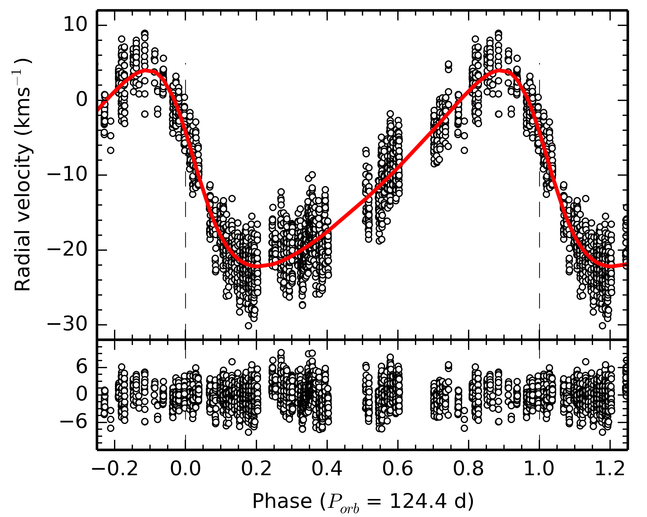
Since the first moment of the line depends somewhat on the wavelength range within which it is calculated, we created five different data sets with different dispersion ranges. We then fitted a Keplerian orbit to each data set. The best solution and errors of the parameters were estimated with a Markov Chain Monte Carlo (MCMC) method implemented in the package emcee (Foreman-Mackey et al., 2013). To account for the scatter due to pulsations, we assumed an uncertainty of (the RMS value of the residuals after subtraction of the binary model, see Table 3) for each radial velocity measurement. To account for the dependence of the radial velocities on the dispersion range, we fitted all five data sets combined. All five models are consistent within the uncertainties of each solution. Figure 2 shows the orbital model fitted to the radial velocities obtained from the dispersion range to and the residuals after subtraction of the mean orbit. The results are shown in Table 3.
Due to the binary motion of the pulsating star we expect the frequencies to show a periodic shift at the base of the orbital period (Shibahashi & Kurtz, 2012, for an explanation of the Doppler shift of oscillation frequencies, see). For the observed photometric frequencies a shift of to can be estimated. Since the analyzed data set has a frequency resolution of , we cannot resolve the expected frequency shifts due to the binary motion. We also did not detect a variation based on the orbital period of the times of maxima in an diagram of the first moment.
From the mean binary orbit, a correction value was calculated for each spectrum to shift the data to the reference frame of the primary. The frequency analysis and mode identification of the pulsations was subsequently performed on the data corrected for the binary motion.
| (days) | 124.44 | 0.03 |
|---|---|---|
| (JD) | 2 454 605 | 10.3 |
| 0.311 | 0.003 | |
| (deg) | 70.2 | 0.7 |
| () | 13.24 | 0.05 |
| () | -10.44 | 0.03 |
| RMS () | 2.8 | |
4 Revision of fundamental parameters
Since the data gathered at McDonald Observatory are limited in wavelength range, we obtained additional observations with the HERMES spectrograph (Raskin et al., 2011), a high-resolution spectrograph () mounted at the 1.2-m Mercator telescope at La Palma, Spain. We obtained three spectra equally spread over the night of the 3rd of February, 2013. The reduction was performed by the HERMES pipeline and normalization was done in the same way as for the McDonald spectra, i.e., by fitting a cubic spline to the continuum region (Pápics et al., 2012). We extracted a wavelength range of to from the data.
For the analysis of the average spectrum of 4 CVn, we used the GSSP program package (Tkachenko et al., 2012; Lehmann et al., 2011). The code relies on a comparison between observed and synthetic spectra computed in a grid of , , micorturbulence , metallicity [m/H], and , and finds the optimum values of these parameters from a minimum in . Individual abundances of chemical elements are adjusted in the second step, by fixing the metallicity to the above determined value but keeping the other atmospheric parameters free. The errors of measurement (1- confidence level) are calculated from the statistics using the projections of the hypersurface of the from all grid points of all parameters onto the parameter in question. For a more detailed discussion on the estimation of the uncertainties, see Tkachenko et al. (2013a). Strong LPVs detected in the spectrum of 4 CVn, as well as possible contributions from the secondary component, are an additional source of uncertainties which are not taken into account in the spectral analysis. Our analysis is based on the grid of atmosphere models computed using the most recent version of the LLmodels code (Shulyak et al., 2004). For the calculation of the synthetic spectra, we used the SynthV code (Tsymbal, 1996), and information on atomic lines has been extracted from the Vienna Atomic Line Database (Kupka et al., 2000, VALD,).
| (K) | 6875 | 120 a aa a aa Parameters derived via spectral analysis. |
|---|---|---|
| (dex) | 3.30 | 0.35 a aa a aa Parameters derived via spectral analysis. |
| (dex) | -0.05 | 0.15 a aa a aa Parameters derived via spectral analysis. |
| (km s-1) | 109 | 3 a aa a aa Parameters derived via spectral analysis. |
| (km s-1) | 4.00 | 0.45 a aa a aa Parameters derived via spectral analysis. |
| ST | F2 III-IV a aa a aa Parameters derived via spectral analysis. | |
| (mas) | 10.51 | 0.40 |
| 1.47 | 0.05 b bb b bb Parameters based on combined photometric and spectroscopic observations. | |
| Radius (R⊙) | 3.7--4.1 b bb b bb Parameters based on combined photometric and spectroscopic observations. | |
| Mass (M⊙) | 1.0--2.0 b bb b bb Parameters based on combined photometric and spectroscopic observations. | |
| Element | Value | Sun | Element | Value | Sun |
|---|---|---|---|---|---|
| dex | dex | dex | dex | ||
| Fe | -4.69(15) | -4.59 | Cr | -6.47(20) | -6.40 |
| Mg | -4.41(25) | -4.51 | Mn | -6.65(40) | -6.65 |
| Ti | -7.24(30) | -7.14 | Si | -4.41(40) | -4.53 |
| Ni | -5.82(20) | -5.73 | C | -3.64(40) | -3.65 |
| Ca | -5.84(25) | -5.73 | Ba | -9.52(50) | -9.87 |
| Sc | -8.57(50) | -8.99 |
Table 4 lists the atmospheric parameters of 4 CVn we derived. The individual abundances of some chemical elements are given in Table 5. The spectral type and the luminosity class have been computed using an interpolation in the tables published by Schmidt-Kaler (1982). Figure 3 compares the observations with the best fit synthetic spectrum in a wide wavelength range including the Hβ spectral line.

Moreover, we used the Hipparcos parallax of 10.51 mas (van Leeuwen, 2007) in combination with 2MASS and Geneva photometry to compute the luminosity and the radius of the star. We used a grid-based method, which also includes interstellar reddening as a free parameter, as described by Degroote et al. (2011). By using the radius and the spectroscopic we are able to estimate the mass. We find an extinction mag. Despite this value being close to zero, adding extinction to the calculations is important for the consistency of our estimated parameters, mass and radius. The results of the photometric analysis are summarised in Table 4.
We also used the above analysed observed spectrum to compute a mean profile with a high S/N by means of the Least-Squares Deconvolution technique (LSD) (Donati et al., 1997; Kochukhov et al., 2010). Figure 4 shows the LSD profile of 4 CVn, the line mask was pre-computed based on the parameters listed in Table 4. Besides clear “bumps” in the center of the profile (dip) of the star, there is also an indication of another broad spectral line at . Whereas the former is connected to the intrinsic variability of the star in terms of (high-degree) non-radial pulsations, the latter might be a signature of a (very) faint stellar companion.

Given the measured semi-amplitude of the primary and the measured systemic velocity , a radial velocity of of the secondary at orbital phase would lead to a mass ratio of . The line strength of the spectral feature around in the LSD profile is . If we assume a minimum contribution of of the secondary to the system luminosity , we estimate , which corresponds to an early M-type main-sequence star of (Carroll & Ostlie, 2006, Appendix G). A mass ratio of would then give a primary mass of , which is too massive given the observed spectral type F2III-IV.
The additional spectral contribution is so faint that it could also be an effect of continuum normalization. As the spectral lines of 4 CVn are broadened by fast rotation (), a continuum is not present everywhere in the wavelength range. Thus, inaccurate continuum normalization is a more likely explanation for the spectral feature at than a secondary signal.
5 Frequency analysis
Before starting the analysis of the data we inspected each spectrum by eye. We rejected 93 observations, due to weak cosmic-ray hits within the line or poor S/N, leaving 2036 (797 in 2008, 758 in 2010, and 481 in 2011) good spectra. Since the periodogram of 4 CVn is characterized by amplitude variations on short and long timescales, we split the whole data set in three parts, studying each season separately. Otherwise the variability of the oscillation pattern would lead to disturbing side peaks in the Fourier spectra and to uncertainties between real frequency peaks and aliasing.
To search for significant periodicities in the LPVs we employed the Fourier-parameter fit method (FPF), which was developed by Zima (2006) as an advancement of the pixel-by-pixel method (Mantegazza, 2000). It is implemented in the software package FAMIAS (Zima, 2008). For each bin in the dispersion range of the line a Fourier transform is performed and a Lomb-Scargle periodogram (Lomb, 1976; Scargle, 1982) is calculated. An optimisation of the mode parameters is done by applying a least-squares fitting algorithm to the original spectra, again, for each bin separately and thereby computing zero point, amplitude, and phase across the line profile. Subsequently, these parameters are used for mode identification (see Sect. 6). A Monte-Carlo perturbation approach has been used to calculate the errors on the amplitudes, assuming a Gaussian distribution of the noise of the amplitude profiles. The S/N of each frequency is calculated from the mean periodogram, prewhitened with the significant frequency peaks. Thereby, the noise () is calculated as the mean amplitude in a range of (covering most of the frequency spectrum) around the frequency peak in the periodogram. We have adopted a significance criterion of (Breger et al., 1993). The results of our analysis are summarized in Table 6.
| Frequency | |||||
|---|---|---|---|---|---|
| d-1 | km s-1 | km s-1 | km s-1 | km s-1 | |
| 7.3764 | 0.953 | 0.95 | 0.98 | 1.00 | |
| 5.8496 | 0.869 | 0.87 | 0.90 | 0.88 | |
| 5.0481 | 0.550 | 0.48 | 0.53 | 0.59 | |
| 8.5942 | 0.444 | 0.48 | 0.51 | 0.33 | |
| 5.5315 | 0.389 | 0.38 | 0.39 | 0.44 | |
| 8.6552 | 0.389 | 0.31 | 0.40 | 0.51 | |
| 8.1687 a aa a aa Frequencies not detected in previous photometric studies. | 0.379 | 0.33 | 0.41 | 0.48 | |
| 6.6801 | whole set, 2010, 2011 | ||||
| 4.0743 a aa a aa Frequencies not detected in previous photometric studies. | whole set, 2010, 2011 c cc c cc Alias peak of frequency detected. | ||||
| 6.1171 | whole set, 2010 | ||||
| 6.975 b bb b bb Photometric radial mode (Lenz et al., 2010). | 2008 | ||||
| 10.1702 a aa a aa Frequencies not detected in previous photometric studies. | whole set, 2010, 2011 | ||||
| 6.1910 | whole set, 2011 | ||||
| 12.4244 a aa a aa Frequencies not detected in previous photometric studies. | whole set, 2010, 2011 | ||||
| 9.4113 a aa a aa Frequencies not detected in previous photometric studies. | whole set, 2008, 2010, 2011 | ||||
| 9.7684 a aa a aa Frequencies not detected in previous photometric studies. | whole set, 2008, 2010 | ||||
| 10.0372 a aa a aa Frequencies not detected in previous photometric studies. | whole set, 2008 | ||||
| 6.4030 | whole set | ||||
| 13.388 a aa a aa Frequencies not detected in previous photometric studies. | 2008 | ||||
| 10.016 a aa a aa Frequencies not detected in previous photometric studies. | 2011 | ||||
5.1 The Fe II line at


The increase in noise towards low frequencies in the periodograms (see Figs. 5, 6, and 7) can be explained by instrumental effects or imperfect subtraction of the binary orbit. Given that the spectrograph is mounted at the telescope and not placed in a remote room where pressure and temperature could be kept constant to avoid spectral drift, some long-term variations are unavoidably present in the data. The high noise level can also be caused by instrumental noise and correlations of different noise sources. Residual variability on the basis of the binary orbit would cause frequency peaks around . For those reasons, we discarded all low-frequency peaks below as being not trustworthy. Furthermore, the daily gaps due to the night-day rhythm led to significant one-day aliasing, which is visible in the spectral window of each season (see inset in the top panel of Figs. 5, 6, and 7 for season 2008, 2010, and 2011, respectively). To overcome these obstacles a prewhitening of each frequency was performed, before carrying out another Fourier transform.
Figures 5, 6, and 7 display the mean of the periodograms that were computed for each bin and for the seasons 2008, 2010, and 2011, respectively. Different stages of prewhitening are shown and the 7 dominant frequencies are marked. We found 6 frequencies that are confirmed by photometric studies and are present in the periodograms of the whole data set and in all three seasons separately as well. These are , , , , , and (Breger, Lenz & Pamyatnykh, in prep.). Other photometrically significant frequencies could be detected in some seasons, while their amplitude was below the detection limit in other subsets. The frequency , for example, could only be detected in 2008. Breger, Lenz & Pamyatnykh (in prep.) confirm a rapid, steady decrease in amplitude for this frequency from 2008 to 2012. Also , , and appear to be varying in amplitude, since they have only been detected in either the season of 2010 or 2011, or in both. However, the amplitude variability we detected for , , and does not agree with the amplitudes derived from the photometric data set. Since these frequencies have a low S/N, their amplitude could also be below the detection limit in other seasons.
Additionally, we found several frequencies, which were not detected in previous photometric studies by Breger et al. (1999); Breger (2000b); Breger et al. (2008), among them , , , and . The frequency can be firmly detected with a comparatively high amplitude () in all sets and subsets. Frequencies , , and have much lower amplitudes, and the amplitudes of and even lie below the detection limit of seasons 2008 and 2011, respectively. The consistency of the detection in the separate seasons and the sufficient S/N for these frequencies in the merged data of the three seasons led us to the conclusion that they correspond to real oscillation frequencies. The fact that these frequencies were not detected in photometry suggests that they are either high-degree modes with or are varying in amplitude and reached detectable amplitudes in the last five years.
Breger et al. (1999) could identify peaks above 10 d-1 as combination frequencies of the main modes between 4 and 10 d-1. The frequencies , , , , and lie in this high frequency range, but could not be confirmed to be combinations of any of the detected frequency peaks with . The amplitude and the phase profiles across the line of a mode offer an additional diagnostic to distinguish between noise peaks and real frequencies. If those profiles show a significant trend and not just random scatter, the frequency is likely to be a real pulsation mode. In Appendix A the amplitude and phase profiles across the line are displayed for the frequencies to . While the amplitude profiles of , , , , and are rather noisy, the phase profiles of these peaks do resemble those of real mode frequencies, i.e., increasing or decreasing from the blue to the red edge of the line. They were thus added to Table 6.
In order to test the influence of the line-cutting limits, we did a frequency analysis using different dispersion ranges for the Fe II line 4508.288 , as explained in Sect. 3. All different values of frequency and amplitude for all five dispersion ranges are consistent within the 1 error bars.
5.2 Analysis of LSD profiles
Due to the high rotation rate of the star, we only found one absorption line to be suitable for performing mode identification. In order to test the potential of using more information from the other spectral lines, we calculated LSD profiles for the McDonald spectra obtained in 2010 with the method by Kochukhov et al. (2010); Tkachenko et al. (2013b). We made use of the line mask, which was computed for Sect. 4, to calculate a standard LSD profile from all the lines in the line mask, as well as an LSD profile of the Fe lines only, using the multi-profile technique, in order to take the blending of Fe-lines into account. Figures 25, 26, and 27 in Appendix B show the mean profile, the standard deviation, and a 2D color image of the LPVs, phase folded onto the frequency , for the Fe II line at , the standard LSD profiles, and the Fe-LSD profiles, respectively.
The shape and depth of an LSD profile depends on the line mask which is used for the computation. As it can be considered as an average of several lines (weak and strong lines of different elements), the depth will typically be less than that of a strong single line, such as Fe II at 4508.288 . Also the overall shape of the LSD profile can differ from that of a single line. All these effects can be seen in the Figures in Appendix B. Note that the amplitude scales in Fig. 25 (single Fe II line) are different from the amplitude scales in Fig. 26 (standard LSD profiles) and Fig. 27 (Fe-LSD profiles). The uneven structure in the continuum region in the lower panels of Figs. 26 and 27 is a consequence of the continuum normalization, which is complicated by the high of 4 CVn. We did not detect any feature in the LSD profiles that is moving according to the orbital period and could be connected to the companion of 4 CVn.

As already explained in Sect. 2.1, different lines can be more or less sensitive to stellar pulsations. It is therefore possible that the pulsation signal is smeared out in an LSD profile. This can affect the phase, but also the amplitude of the pulsation modes. Figure 8 depicts the mean amplitude spectra for the Fe II line 4508.288 (grey) and for the standard LSD profiles (black). In order to compare the two periodograms, we had to rescale the LSD profiles to match the amplitude of the Fe II line, as the pulsation amplitudes are expressed in units relative to the continuum of the line. The noise level in the periodogram of the rescaled LSD profiles is only lower in the low-frequency range and it contains less pulsation signal than the periodogram of the single line. This is reflected in the number of detected frequencies. While we could detect 14 significant () frequencies in the LPVs of Fe II (Table 6), we could only find 8 of them in the LPVs of the LSD profile. The frequencies detected in the LSD profiles had a lower S/N, and the amplitudes dropped by almost for and by for .
The results are similar for the LSD profiles based only on the Fe lines. The noise level in the mean periodogram of the Fe-LSD profiles is slightly higher than in the mean periodogram of the standard LSD profiles, since less lines were used for the computation of the profiles. Consequently, the amplitudes and S/N of the detected frequencies are even lower than the values found from the analysis of the standard LSD profiles.
As the LSD profiles do not yield any improvement to the single line, we conducted the further analysis on the Fe II line 4508.288 . It was already stressed by Aerts et al. (2010, Chapter 4) that line-profile analysis works best on one carefully selected, isolated line, if available.
6 Mode identification
6.1 Fourier-parameter fit method
During the frequency analysis (see Sect. 5) the observed Fourier parameters zero point , amplitude , and phase across the line were obtained for each oscillation frequency. For mode identification the observed profiles are compared to theoretical profiles. Possible solutions can be compared by calculating a reduced . The theoretical values are computed from synthetic line profiles, which result from an integration over a surface grid divided into segments. The intrinsic profile of each surface element is assumed to be Gaussian, and the local variations of flux arise from variations of temperature and surface gravity. Temperature variations, which lead to a varying equivalent width , are neglected in a first approximation. Thus, we can also neglect the dependence of equivalent width on temperature and assume a constant . The method is described in detail by Zima (2006, and references therein); Zima (2008, and references therein).
To obtain accurate mode identification, the FPF method requires the input of stellar parameters, such as mass, radius, metallicity, temperature, and surface gravity. Besides giving a solution for it also allows us to derive parameters of the line that are independent of pulsation, like, equivalent width (only in first approximation), the width of the intrinsic Gaussian profile , and the velocity offset , which is a measure of radial velocity. Additionally the inclination angle between pulsation axis and line-of-sight as well as the projected rotational velocity can be derived.
We recall that the method is most powerful to determine the -values and not so much the -values (Zima, 2008).
6.2 Mode identification of and
Mode identification has been carried out for the two dominant frequencies and . We folded the series of spectra on the phase of and , respectively, and smoothed the LPVs in 50 phase bins. In this way we remove the signal of the several other p-modes which are excited with very low amplitudes and whose frequencies are hard to distinguish from noise and can therefore not be extracted from the data. Hence, we are able to treat the star as a mono-periodic pulsator during the mode identification. The zero point, amplitude, and phase profiles across the line obtained from the phase-folded data set are displayed in Figs. 9 and 10 for and , respectively.


We found the solution for . For , mode identification was ambiguous; and are the best fits to depending on the stellar input parameters. However, other solutions cannot be excluded for both and , since the differs by only a few percent. Furthermore, we receive a high () for all and combinations, which means that no solution provides a good fit to the observations. This will be discussed in Sect. 7. All results are summarized in Appendix C, in Tables 10, 11, and 12. Figures 30, 30, 30, 33, 33, and 33 show the observed amplitude and phase profile of fitted with the modes , , , , , and , respectively. The fits to the observed amplitude and phase profile of with the modes , , , , , and are shown in Figs. 36, 36, 36, 39, 39, and 39, respectively.
6.2.1 Line-profile parameters
Before fitting amplitude and phase across the line to identify the modes, the pulsation-independent line-profile parameters, projected rotational velocity , equivalent width , the width of the intrinsic Gaussian profile , and the velocity offset of the line center at 0 km s-1 are constrained by fitting the zero-point profile with a non-pulsating model. However, these parameters varied when fitting the pulsation modes and were therefore left as free parameters during the mode identification. The ranges within which the fits were computed are summarized in Table 7.
| Central wavelength () | 4508.288 |
|---|---|
| (km s-1) | 106.0–107.3 |
| (km s-1) | 15.0–15.25 |
| (km s-1) | 8.0–9.5 |
| (km s-1) | –0.5 |
6.2.2 Three sets of stellar input parameters
The photometric and spectroscopic analysis, presented in Sect. 4, suggests that the mass of 4 CVn lies between 1 and 2 M⊙, while the radius is between 3.7 and 4.1 R⊙. The effective temperature of the star , the surface gravity dex, and the metallicity is near solar.
Breger & Pamyatnykh (2002) computed a model with the 18 photometrically observed frequencies of 4 CVn, assuming , , , , , and solar metallicity. The luminosity of this model is a factor of 2 higher than our deduced value .
Since the stellar parameters are not well constrained, we calculated the mode identification for three different sets of parameters, which are summarized in Table 8. The values of set 1 and set 2 lie within the ranges of the results of our spectroscopic and photometric analysis, while the values for set 3 are based on the model by Breger & Pamyatnykh (2002). The inclination angle, , was fitted within the range . We adopted a lower limit , as it is the critical value, where the star rotates at the break-up velocity (Townsend et al., 2004, , where is the equatorial radius;). The critical velocity , which depends on the stellar mass and radius, is also given for each set in Table 8.
It is not possible to distinguish between the three sets of stellar parameters. The best solutions of all three sets lie within of and are therefore equally possible. For , the best fitting combination is always a mode. The solution for , however, shows a dependence on the stellar input parameters and differs for the three different sets (see Tables 10, 11, 12).
| Set 1 a aa a aa Values based on our spectroscopic and photometric analysis (see Sect. 4). | Set 2 a aa a aa Values based on our spectroscopic and photometric analysis (see Sect. 4). | Set 3 b bb b bb Values based on Breger & Pamyatnykh (2002). | |
| Mass () | 2.0 | 1.5 | 2.4 |
| Radius () | 3.72 | 3.75 | 5.6 |
| () | 7050 | 6950 | 6800 |
| (dex) | 3.6 | 3.45 | 3.32 |
| (dex) | 0 | 0 | 0 |
| c cc c cc The critical velocity is given by . | 320.3 | 276.3 | 286.0 |
| Inclination (deg) | 23–90 | ||
6.2.3 Inclination angle
For our computations, we assume that the pulsation axis coincides with the rotation axis. The inclination angle is then the angle between this axis and the line-of-sight. It is thus not physically possible that and are observed at a different . However, in Tables 10, 11, and 12 it can be seen that the value of varies between the solutions for the different sets of stellar parameters and the two frequencies. This is also illustrated in Fig. 11. Displayed are, from top to bottom, the distribution of for set 1, set 2, and set 3 of stellar parameters, respectively. The minimum value is shown for each bin in inclination for (blue squares) and (green diamonds) in each panel. For set 3 the frequencies and show an opposite behavior. While favors higher inclination values around to , mode identification for yields . Set 1 and set 2 give a more consistent result for , where and follow the same trend. On the other hand, there is also no clear minimum visible in , neither for nor for in any of the three sets. The inclination is highly degenerate with the degree and the order of the oscillation mode, as it determines the visibility of a certain mode. Mode identification was ambiguous for and and certain effects hamper us from drawing clear conclusions, as will be discussed in Sect. 7. Thus, we can also not find a consistent inclination for 4 CVn.

6.2.4 Temperature and equivalent-width variations
So far we ignored variations of temperature in a first approximation and assumed a constant ; thus, .
To improve the fits of the amplitude and phase profiles we varied the parameter and other parameters related to the temperature dependence of the flux variation; at first within a very broad range, and gradually narrowing down the range. However, the parameters did not converge and the minimum in varied with each iteration, without improving the overall significantly. The final solution therefore had to be calculated with , neglecting temperature variations.
| Frequency | ||
|---|---|---|
| 7.3764 | retrograde | |
| 5.8496 | prograde | |
| 5.0481 | retrograde or axisymmetric | |
| 5.5315 | prograde | |
| 8.5942 | prograde | |
| 8.6552 | prograde | |
| 8.1688 | high-degree, prograde | |
6.3 Azimuthal order of the 7 most-dominant frequencies
Mode identification has also been attempted for the frequencies , , , , and . However, the amplitude of decreases by almost compared to and the amplitudes of the other frequencies are even lower. Therefore, phase folding of the spectra on the respective frequencies and smoothing the LPVs in phase bins did not remove the signal of the two most-dominant frequencies sufficiently. A consistent mode identification can thus not be achieved.
However, as the FPF method is sensitive to phase, the slope of the phase profile across the line allows us to distinguish between prograde (Zima, 2008, i.e., a wave traveling in the direction of rotation; positive , following the definition by), retrograde (negative ), and axisymmetric () modes. Our results are displayed in Table 9.
We also attempted mode identification for . Our results do not contradict the solution presented in Lenz et al. (2010), who reported that it is a radial mode.
The very complex amplitude and phase profiles of , i.e., containing many bumps, suggests that it is a high-degree mode, with . For modes with a high value, partial cancellation would lead to very low amplitudes in photometric observations, where the brightness variation integrated over the stellar disk is measured. This mode was not detected in photometric data before, which supports our hypothesis of a high for .
7 Discussion
7.1 Mode visibility and rotational splitting
The mode identification we attempted for the star 4 CVn did not yield unambiguous results. The statistics give several possible solutions for and , depending on the stellar input parameters. For frequency the best solution yields and for frequency , or . Theory predicts that modes with degree cancel out almost completely in photometric observations (Aerts et al., 2010, Chapter 6). However, both and were detected with significant amplitudes in photometric data (see Table 1), which contradicts the results of our mode identification. The solutions and would be in best agreement with the current theory and our results.
We, therefore, tested the hypothesis that and are the outer parts of a rotationally split quintuplet. Rotational splitting (Ledoux, 1951) describes the shift of frequencies of modes of same degree and different order () due to the Coriolis force. It is dependent on and the rotational period of the star. With set 3 of stellar parameters and it would be possible that we are observing rotational splitting in 4 CVn (see Table 12 and Fig. 11).
7.2 Rotation rate
We conclude that 4 CVn rotates at a significant fraction of its critical velocity. We measured a projected rotational velocity for the star. Thus, its equatorial velocity is at least of its critical velocity . Since the inclination angle and the stellar mass and radius are poorly constrained, it is possible that it rotates at up to almost of . Tables 10, 11, and 12 display the possible ranges of and .
Reese et al. (2013) showed that even a moderate rotation rate has large effects on the visibility of oscillation modes. While partial cancellation makes modes almost not detectable in photometric data for slow rotation (), their amplitudes are as high as the amplitudes of modes with if (Reese et al., 2013, see Fig. 7 of). This would mean that our results of for and do not contradict the mode amplitudes observed in photometric light curves. However, fast rotation also alters the geometry of the modes (Reese et al., 2009). Since higher-order effects of rotation are not yet included in the methodology for mode identification, this could be an explanation for the poor fits we obtained. If this is the case, the amplitude and phase profiles across the line, as well as the amplitude ratios of multi-color photometry would have to be revisited, with a methodology that includes the effects of rotation on the pulsation modes.
8 Summary
In this work, we analyzed the line-profile variations of the Sct star 4 CVn based on the spectroscopic observations obtained between January 2008 and June 2011 at McDonald Observatory, Texas, USA. We discovered that the star is the primary component of an eccentric binary system with an orbital period d and eccentricity . No signal of the secondary could be detected in our data. The frequency analysis revealed 20 oscillation modes, 11 of which were already detected in photometric data sets by Breger et al. (1999); Breger (2000b); Breger et al. (2008).
By phase-folding the series of spectra onto the two dominant frequencies and , respectively and smoothing the LPVs in phase bins, we removed the signal of other periodicities to prepare the data for mode identification. The best solution for frequency is an mode, while the best solution for was either or depending on the stellar input parameters. For the calculations of the synthetic LPVs we used three different sets of stellar parameters:
- 1.
, , K, , and [m/H]=0.
- 2.
, , K, , and [m/H]=0.
- 3.
, , K, , and [m/H]=0.
Set 1 and 2 are based on the spectroscopic and photometric analysis we performed to revise the stellar parameters. Set 3 is based on a model calculated by Breger & Pamyatnykh (2002). No set of stellar parameters can be excluded, based on the statistics.
Relying on previous results by Castanheira et al. (2008), Breger (2010) claimed a relationship between the frequency variations of 4 CVn and the azimuthal order of the modes, and especially the direction of the running wave (retrograde, prograde or axisymmetric/radial modes). The FPF method is most sensitive to the sign of . Our results in Table 9 are in agreement with the directions of the waves used by Breger (2010).
The star is a fast rotator with a projected rotational velocity . Depending on the stellar input parameters and the inclination angle (which could not be constrained), the star is rotating at of the critical velocity . The higher-order effects of rotation were not taken into account in our analysis, since they are not yet included in the methodology for mode identification.
A further limitation from the methodology is that unblended metal lines have to be used for mode identification. However, our observed spectral range (4500 to 4700 ) is a very dense spectral region with many absorption lines and very little continuum for F stars, and almost all absorption lines are (heavily) blended. In an attempt to solve this problem, we calculated LSD profiles from the McDonald spectra, obtained in the season 2010. We found that the pulsation signal is smeared out in the LSD profiles, as the number of significant oscillation modes detected in the LPVs of the LSD profiles is less than for the single Fe II line. Also the amplitudes and the S/N levels of these modes are reduced significantly. To improve our analysis a method to identify the modes in blended lines would have to be developed. Also, observations in a wider spectral range could help solve the problem of blended lines. The lines that Zima et al. (2006) used for their analysis of the Sct star FG Vir, lie outside the observed spectral range of the McDonald data. Observing a wider spectral range with a stable, high-resolution spectrograph would allow to follow up on the additional spectral feature detected in the LSD profile of 4 CVn (see Fig. 4), and could possibly lead to identification of the origin of the latter.
Accurate mode identification of many observed frequencies is a crucial input for successful modeling of stellar oscillations. Analyses of LPVs are important as they can constrain the azimuthal order of the pulsation modes. However, current shortcomings in the methodology prevent unambiguous and accurate mode identification for 4 CVn. Including a complete description of rotation and the use of blended lines into mode-identification techniques will make this possible in the future.
Acknowledgements.
This research has received funding from the Fonds zur Förderung der wissenschaftlichen Forschung (FWF), Austria P17441-N02, from the European Community’s Seventh Framework Programme FP7-SPACE-2011-1, project number 312844 (SPACEINN), as well as from the Belgian Science Policy Office (Belspo, C90309: CoRoT Data Exploitation). It is partly based on observations made with the Mercator Telescope, operated on the island of La Palma by the Flemish Community, at the Spanish Observatorio del Roque de los Muchachos of the Instituto de Astrofísica de Canarias and obtained with the HERMES spectrograph, which is supported by the Fund for Scientific Research of Flanders (FWO), Belgium , the Research Council of KU Leuven, Belgium, the Fonds National Recherches Scientific (FNRS), Belgium, the Royal Observatory of Belgium, the Observatoire de Genève, Switzerland and the Thüringer Landessternwarte Tautenburg, Germany. SB is supported by the Foundation for Fundamental Research on Matter (FOM), which is part of the Netherlands Organisation for Scientific Research (NWO).References
- Aerts et al. (2010) Aerts, C., Christensen-Dalsgaard, J., & Kurtz, D. W. 2010, Asteroseismology, 1st edn. (Springer), 866
- Aerts et al. (1992) Aerts, C., de Pauw, M., & Waelkens, C. 1992, A&A, 266, 294
- Antoci et al. (2011) Antoci, V., Handler, G., Campante, T. L., et al. 2011, Nature, 477, 570
- Auvergne et al. (2009) Auvergne, M., Bodin, P., Boisnard, L., et al. 2009, A&A, 506, 411
- Borucki et al. (2010) Borucki, W. J., Koch, D., Basri, G., et al. 2010, Science, 327, 977
- Breger (2000a) Breger, M. 2000a, in Astronomical Society of the Pacific Conference Series, Vol. 210, Delta Scuti and Related Stars, ed. M. Breger & M. Montgomery, 3
- Breger (2000b) Breger, M. 2000b, MNRAS, 313, 129
- Breger (2010) Breger, M. 2010, in Variable Stars, the Galactic halo and Galaxy Formation, ed. C. Sterken, N. Samus, & L. Szabados, 95
- Breger & Bischof (2002) Breger, M. & Bischof, K. M. 2002, A&A, 385, 537
- Breger et al. (2008) Breger, M., Davis, K. A., & Dukes, R. J. 2008, Communications in Asteroseismology, 153, 63
- Breger et al. (1999) Breger, M., Handler, G., Garrido, R., et al. 1999, A&A, 349, 225
- Breger & Pamyatnykh (2002) Breger, M. & Pamyatnykh, A. A. 2002, in Astronomical Society of the Pacific Conference Series, Vol. 259, IAU Colloq. 185: Radial and Nonradial Pulsationsn as Probes of Stellar Physics, ed. C. Aerts, T. R. Bedding, & J. Christensen-Dalsgaard, 388
- Breger & Pamyatnykh (2006) Breger, M. & Pamyatnykh, A. A. 2006, MNRAS, 368, 571
- Breger et al. (1993) Breger, M., Stich, J., Garrido, R., et al. 1993, A&A, 271, 482
- Carroll & Ostlie (2006) Carroll, B. W. & Ostlie, D. A. 2006, An Introduction to Modern Astrophysics, 2nd edn. (Addison-Wesley), 1400
- Castanheira et al. (2008) Castanheira, B. G., Breger, M., Beck, P. G., et al. 2008, Communications in Asteroseismology, 157, 124
- Degroote et al. (2011) Degroote, P., Acke, B., Samadi, R., et al. 2011, A&A, 536, A82
- Donati et al. (1997) Donati, J.-F., Semel, M., Carter, B. D., Rees, D. E., & Collier Cameron, A. 1997, MNRAS, 291, 658
- Foreman-Mackey et al. (2013) Foreman-Mackey, D., Hogg, D. W., Lang, D., & Goodman, J. 2013, PASP, 125, 306
- Grevesse et al. (2007) Grevesse, N., Asplund, M., & Sauval, A. J. 2007, Space Sci. Rev., 130, 105
- Grigahcène et al. (2010) Grigahcène, A., Antoci, V., Balona, L., et al. 2010, ApJ, 713, L192
- Kochukhov et al. (2010) Kochukhov, O., Makaganiuk, V., & Piskunov, N. 2010, A&A, 524, A5
- Kupka et al. (2000) Kupka, F. G., Ryabchikova, T. A., Piskunov, N. E., Stempels, H. C., & Weiss, W. W. 2000, Baltic Astronomy, 9, 590
- Ledoux (1951) Ledoux, P. 1951, ApJ, 114, 373
- Lehmann et al. (2011) Lehmann, H., Tkachenko, A., Semaan, T., et al. 2011, A&A, 526, A124
- Lenz et al. (2010) Lenz, P., Pamyatnykh, A. A., & Breger, M. 2010, in Variable Stars, the Galactic halo and Galaxy Formation, ed. C. Sterken, N. Samus, & L. Szabados, 83
- Lomb (1976) Lomb, N. R. 1976, Ap&SS, 39, 447
- Mantegazza (2000) Mantegazza, L. 2000, in Astronomical Society of the Pacific Conference Series, Vol. 210, Delta Scuti and Related Stars, ed. M. Breger & M. Montgomery, 138
- McCarthy et al. (1993) McCarthy, J. K., Sandiford, B. A., Boyd, D., & Booth, J. 1993, PASP, 105, 881
- Murphy et al. (2013) Murphy, S. J., Pigulski, A., Kurtz, D. W., et al. 2013, MNRAS, 432, 2284
- Pápics et al. (2012) Pápics, P. I., Briquet, M., Baglin, A., et al. 2012, A&A, 542, A55
- Raskin et al. (2011) Raskin, G., van Winckel, H., Hensberge, H., et al. 2011, A&A, 526, A69
- Reese et al. (2009) Reese, D. R., MacGregor, K. B., Jackson, S., Skumanich, A., & Metcalfe, T. S. 2009, A&A, 506, 189
- Reese et al. (2013) Reese, D. R., Prat, V., Barban, C., van ’t Veer-Menneret, C., & MacGregor, K. B. 2013, A&A, 550, A77
- Scargle (1982) Scargle, J. D. 1982, ApJ, 263, 835
- Shibahashi & Kurtz (2012) Shibahashi, H. & Kurtz, D. W. 2012, MNRAS, 422, 738
- Shulyak et al. (2004) Shulyak, D., Tsymbal, V., Ryabchikova, T., Stütz, C., & Weiss, W. W. 2004, A&A, 428, 993
- Tkachenko et al. (2012) Tkachenko, A., Lehmann, H., Smalley, B., Debosscher, J., & Aerts, C. 2012, MNRAS, 422, 2960
- Tkachenko et al. (2013a) Tkachenko, A., Lehmann, H., Smalley, B., & Uytterhoeven, K. 2013a, MNRAS, 431, 3685
- Tkachenko et al. (2013b) Tkachenko, A., Van Reeth, T., Tsymbal, V., et al. 2013b, A&A, 560, A37
- Townsend et al. (2004) Townsend, R. H. D., Owocki, S. P., & Howarth, I. D. 2004, MNRAS, 350, 189
- Tsymbal (1996) Tsymbal, V. 1996, in Astronomical Society of the Pacific Conference Series, Vol. 108, M.A.S.S., Model Atmospheres and Spectrum Synthesis, ed. S. J. Adelman, F. Kupka, & W. W. Weiss, 198
- Uytterhoeven et al. (2011) Uytterhoeven, K., Moya, A., Grigahcène, A., et al. 2011, A&A, 534, A125
- van Leeuwen (2007) van Leeuwen, F. 2007, A&A, 474, 653
- Walker et al. (2003) Walker, G., Matthews, J., Kuschnig, R., et al. 2003, PASP, 115, 1023
- Zima (2006) Zima, W. 2006, A&A, 455, 227
- Zima (2008) Zima, W. 2008, Communications in Asteroseismology, 155, 17
- Zima et al. (2006) Zima, W., Wright, D., Bentley, J., et al. 2006, A&A, 455, 235
Appendix A Amplitude and phase profiles


Appendix B Comparison of LSD profiles and single-line profiles


Appendix C Results of the mode identification of and
| (deg) | (km s-1) | (km s-1) | (deg) | (km s-1) | (km s-1) | ||||||
| 66.3 | 106.5 | 116.3 | 0.36 | 28.6 | 61.0 | 106.9 | 122.2 | 0.38 | 29.0 | ||
| 88.9 | 106.7 | 106.7 | 0.33 | 29.7 | 36.2 | 106.8 | 180.8 | 0.56 | 30.8 | ||
| 41.5 | 106.6 | 160.9 | 0.50 | 34.6 | 51.5 | 106.6 | 136.2 | 0.43 | 35.3 | ||
| 51.5 | 106.6 | 136.2 | 0.43 | 38.3 | 44.1 | 106.8 | 153.5 | 0.48 | 39.6 | ||
| 38.3 | 106.5 | 171.8 | 0.54 | 47.7 | 35.1 | 106.7 | 185.6 | 0.58 | 65.6 | ||
| 43.6 | 106.6 | 154.6 | 0.48 | 68.7 | 24.6 | 106.7 | 256.3 | 0.80 | 68.3 | ||
| (deg) | (km s-1) | (km s-1) | (deg) | (km s-1) | (km s-1) | ||||||
| 61.5 | 106.7 | 121.4 | 0.44 | 28.7 | 38.3 | 106.9 | 172.5 | 0.62 | 30.4 | ||
| 90.0 | 106.8 | 106.8 | 0.39 | 30.5 | 34.1 | 107.0 | 190.9 | 0.69 | 30.8 | ||
| 43.0 | 106.7 | 156.5 | 0.57 | 36.0 | 36.7 | 106.9 | 178.9 | 0.65 | 36.8 | ||
| 58.3 | 106.8 | 125.5 | 0.45 | 38.5 | 48.9 | 106.6 | 141.5 | 0.51 | 39.1 | ||
| 43.0 | 106.6 | 156.3 | 0.57 | 47.7 | 34.1 | 106.8 | 190.5 | 0.69 | 64.0 | ||
| 43.6 | 106.7 | 154.7 | 0.56 | 69.1 | 23.0 | 106.7 | 273.1 | 0.99 | 66.9 | ||
| (deg) | (km s-1) | (km s-1) | (deg) | (km s-1) | (km s-1) | ||||||
| 69.4 | 106.8 | 114.1 | 0.40 | 29.7 | 31.5 | 107.0 | 204.8 | 0.72 | 31.6 | ||
| 87.9 | 107.0 | 107.1 | 0.37 | 31.6 | 79.4 | 106.5 | 108.3 | 0.38 | 34.0 | ||
| 42.0 | 106.8 | 159.6 | 0.56 | 37.4 | 23.0 | 107.2 | 274.4 | 0.96 | 43.8 | ||
| 57.8 | 106.9 | 126.3 | 0.44 | 38.7 | 40.9 | 107.0 | 163.4 | 0.57 | 44.3 | ||
| 44.1 | 106.8 | 153.5 | 0.54 | 48.5 | 30.9 | 107.0 | 208.4 | 0.73 | 57.4 | ||
| 43.6 | 106.9 | 155.0 | 0.54 | 69.1 | 23.0 | 107.0 | 273.8 | 0.96 | 61.7 | ||


