The List Coloring Reconfiguration Problem
for Bounded Pathwidth Graphs
Abstract
We study the problem of transforming one list (vertex) coloring of a graph into another list coloring by changing only one vertex color assignment at a time, while at all times maintaining a list coloring, given a list of allowed colors for each vertex. This problem is known to be PSPACE-complete for bipartite planar graphs. In this paper, we first show that the problem remains PSPACE-complete even for bipartite series-parallel graphs, which form a proper subclass of bipartite planar graphs. We note that our reduction indeed shows the PSPACE-completeness for graphs with pathwidth two, and it can be extended for threshold graphs. In contrast, we give a polynomial-time algorithm to solve the problem for graphs with pathwidth one. Thus, this paper gives precise analyses of the problem with respect to pathwidth.
1 Introduction
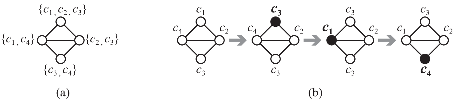
Graph coloring is one of the most fundamental research topics in the field of theoretical computer science. Let be the set of colors. A (proper) -coloring of a graph is a mapping such that for every edge . In list coloring, each vertex has a set of colors, called the list of . Then, a -coloring of is called a -list coloring of if holds for every vertex . Figure 1(b) illustrates four -list colorings of the same graph with the same list depicted in Figure 1(a); the color assigned to each vertex is attached to the vertex. Clearly, a -coloring of is a -list coloring of for which holds for every vertex of , and hence -list coloring is a generalization of -coloring.
Graph coloring has several practical applications, such as in scheduling, frequency assignments. For example, in the frequency assignment problem, each vertex corresponds to a base station and each edge represents the physical proximity and hence the two corresponding base stations have the high potential of interference. Each color represents a channel of a particular frequency, and we wish to find an assignment of channels to the base stations without any interference. Furthermore, in list coloring, each base station can have a list of channels that can be assigned to it.
1.1 Our problem
However, a practical issue in channel assignments requires that the formulation should be considered in more dynamic situations. One can imagine a variety of practical scenarios where a -list coloring (e.g., representing a feasible channel assignment) needs to be transformed (to use a newly found better solution or to satisfy new side constraints) by individual color changes (keeping the network functionality and preventing the need for any coordination) while maintaining feasibility (so that the users receive service even during the reassignment).
In this paper, we thus study the following problem: Suppose that we are given two -list colorings of a graph (e.g., the leftmost and rightmost ones in Figure 1(b)), and we are asked whether we can transform one into the other via -list colorings of such that each differs from the previous one in only one vertex color assignment. We call this decision problem the -list coloring reconfiguration problem. For the particular instance of Figure 1(b), the answer is “yes,” as illustrated in Figure 1(b), where the vertex whose color assignment was changed from the previous one is depicted by a black circle.
1.2 Known and related results
Recently, similar settings of problems have been extensively studied in the framework of reconfiguration problems [13], which arise when we wish to find a step-by-step transformation between two feasible solutions of a problem such that all intermediate solutions are also feasible. This reconfiguration framework has been applied to several well-studied combinatorial problems, including satisfiability [11, 21], independent set [6, 12, 13, 20, 22], set cover, matching [13], shortest path [3, 4, 19], list edge-coloring [14, 16], list -labeling [15], and so on.
In particular, the -coloring reconfiguration problem (i.e., -list coloring reconfiguration in which holds for every vertex ) is one of the most well-studied reconfiguration problems, from the various viewpoints [1, 2, 5, 7, 10, 18, 25], as follows.
Bonsma and Cereceda [5] proved that -coloring reconfiguration is PSPACE-complete for ; they also proved that -list coloring reconfiguration is PSPACE-complete, even for bipartite planar graphs and . On the other hand, Cereceda et al. [10] proved that -coloring reconfiguration is solvable for any graph in polynomial time for the case where .
Then, some sufficient conditions have been proposed so that any pair of -colorings of a graph has a desired transformation. Cereceda [9] gave a sufficient condition with respect to the number of colors: if is at least the treewidth of a graph plus two, then there is a desired transformation between any pair of -colorings of ; the length of the transformation (i.e., the number of recoloring steps) is estimated by Bonamy and Bousquet [2]. Bonamy et al. [1] gave a sufficient condition with respect to graph structures: for example, chordal graphs and chordal bipartite graphs satisfy their sufficient condition.
Recently, Bonsma et al. [7] and Johnson et al. [18] independently developed a fixed-parameter algorithm to solve -coloring reconfiguration when parameterized by , where is the number of colors and is the number of recoloring steps. In contrast, if the problem is parameterized only by , then it is W[1]-hard [7] and does not admit a polynomial kernelization unless the polynomial hierarchy collapses [18].
In this way, even for the non-list version, only a few results are known from the viewpoint of polynomial-time solvability. Furthermore, as far as we known, no algorithmic result has been obtained for the list version.
1.3 Our contribution
In this paper, we study the -list coloring reconfiguration problem from the viewpoint of graph classes, especially pathwidth of graphs. (The definition of pathwidth will be given in Section 2.)
We first show that the problem remains PSPACE-complete even for graphs with pathwidth two. In contrast, we give a polynomial-time algorithm to solve the problem for graphs with pathwidth one. Thus, this paper gives precise analyses of the problem with respect to pathwidth.
Indeed, our reduction for the PSPACE-completeness proof constructs a bipartite series-parallel graph (whose treewidth is two), which is a bipartite planar graph. We note that the problem of finding one -list coloring of a given graph can be solved in polynomial time for bounded treewidth graphs (and hence for bounded pathwidth graphs) [17]. However, our proof shows that the reconfiguration variant is PSPACE-complete even if treewidth and pathwidth are two. Furthermore, as a byproduct, our reduction can be extended for threshold graphs.
2 Preliminaries
We assume without loss of generality that graphs are simple and connected. Let be a graph with vertex set and edge set ; we sometimes denote by and the vertex set and edge set of , respectively. For a vertex in , we denote by the degree of in . For a vertex subset , we denote by the subgraph of induced by .
We now define the notion of pathwidth [24]. A path-decomposition of a graph is a sequence of subsets of vertices in such that
- (1)
;
- (2)
for each , there is at least one subset with ; and
- (3)
for any three indices such that , .
The width of a path-decomposition is defined as , and the pathwidth of is the minimum such that has a path-decomposition of width .
To develop our algorithm in Section 4, it is important to notice that every connected graph of pathwidth one is a caterpillar [23]. A caterpillar will be defined in Section 4, but an example can be found in Figure 4.
For a graph with a list , we define the reconfiguration graph as follows: each node of corresponds to a -list coloring of , and two nodes of are joined by an edge if their corresponding -list colorings and satisfy , that is, can be obtained from by changing the color assignment of a single vertex . We will refer to a node of in order to distinguish it from a vertex of . Since we have defined -list colorings as the nodes of , we use graph terms such as adjacency and path for -list colorings. For notational convenience, we sometimes identify a node of with its corresponding -list coloring of if it is clear from the context.
Given a graph with a list and two -list colorings and of , the -list coloring reconfiguration problem asks whether the reconfiguration graph has a path between the two nodes and .
3 PSPACE-completeness
In this section, we first prove that the problem is PSPACE-complete even for graphs with pathwidth two. Then, we show in Section 3.3 that the reduction can be extended to proving the PSPACE-completeness of threshold graphs.
A graph is series-parallel if it does not contain a subdivision of a complete graph on four vertices [8]. Note that series-parallel graphs may have super-constant pathwidth, although their treewidth can be bounded by two. We give the following theorem.
Theorem 3.1
The -list coloring reconfiguration problem is PSPACE-complete even for bipartite series-parallel graphs of pathwidth two.
It is known that -list coloring reconfiguration is in PSPACE [5]. Therefore, as a proof of Theorem 3.1, we give a polynomial-time reduction from the shortest path rerouting problem [4] (defined in Section 3.1) to our problem for bipartite series-parallel graphs of pathwidth two.
3.1 Reconfiguration problem for shortest path
Let be an unweighted graph, and let and be two vertices in . We call a shortest path in between and simply an S-path in . Note that, since is unweighted, an S-path indicates a path between and having the minimum number of edges. We say that two S-paths and in are adjacent if they differ in exactly one vertex, that is, and hold. Given two S-paths and in , the shortest path rerouting problem asks whether there exists a sequence of S-paths such that , and and are adjacent for each . This problem is known to be PSPACE-complete [4].
To construct our reduction, we introduce some terms. Let be the number of edges of an S-path in a graph . For two vertices and in , we denote by the number of edges of a shortest path in between and ; then . For each , the layer from is defined to be the set of all vertices in that are placed at distance from , that is, . Similarly, let for each . Then, for each , the layer of is defined as follows: . Notice that any S-path in contains exactly one vertex from each layer , . Then, observe that two S-paths and in are adjacent if and only if there exists exactly one index such that . Therefore, we may assume without loss of generality that consists of only vertices in , as illustrated in Figure 2(a). In the example of Figure 2(a), all vertices in the same layer are depicted by the same shape, that is, , , , and . Note that both and always hold.
3.2 Reduction
Given an instance of shortest path rerouting, we construct the corresponding instance of -list coloring reconfiguration.

Construction of and .
We first construct the corresponding graph with a list . For each , let ; and we introduce a vertex , called a layer vertex, to . The list of each layer vertex is defined as , where each color in corresponds to the vertex in ; assigning color represents selecting the vertex as an S-path in . We denote by the set of all layer vertices in . In Figure 2(b), each layer vertex is illustrated as a black vertex which is the same shape as the vertices in .
We then connect layer vertices in by forbidden paths of length two, as follows. Let and be an arbitrary pair of vertices in such that . We introduce a vertex to , and join and each of the two layer vertices and by an edge. The list of consists of two colors and which correspond to the vertices and in , respectively. (See the vertices depicted by white circles in Figure 2(b).) We call such a vertex in a -forbidden vertex or simply a forbidden vertex. Notice that there is no proper -list coloring such that and ; otherwise there is no color in that can be assigned to . This property ensures that every -list coloring of corresponds to an S-path in . Let be the set of all forbidden vertices, then where is the complement graph of .
This completes the construction of and . Since and , we can construct in polynomial time. Clearly, is a bipartite series-parallel graph of pathwidth two, whose bipartition consists of and .
Construction of and .
We now construct two -list colorings and of which correspond to S-paths and in , respectively. For each , let be the vertex in the layer passed through by the S-path ; then we let for each layer vertex . For each -forbidden vertex , we choose an arbitrary color from and which is assigned to neither nor . We note that such an available color always exists, because has an edge between the two vertices corresponding to the colors and , and hence at least one of and holds for each -forbidden vertex. Similarly, we construct . This completes the construction of the corresponding instance .
Correctness of the reduction.
To show the correctness of this reduction, we give the following lemma.
Lemma 1
is a yes-instance if and only if is a yes-instance.
Proof
We first prove the if-part. Suppose that the reconfiguration graph has a path between the two nodes and . We can classify the recoloring steps into the following two types: (1) recoloring a layer vertex in , and (2) recoloring a forbidden vertex in . Therefore, the path in can be divided into sub-paths, intermittently at each edge corresponding to a recoloring step of type (1) above; all edges in a sub-path correspond to recoloring steps of type (2) above. Therefore, all nodes in each sub-path correspond to the same S-path in . Furthermore, any two consecutive sub-paths correspond to two adjacent S-paths (that differ in only one vertex), because the sub-paths are divided by a recoloring step of type (1). Thus, we can construct a sequence of adjacent S-paths that transforms into .
We then prove the only-if-part. Suppose that there exists a sequence of S-paths such that , and and are adjacent for each . For two adjacent S-paths and , , assume that is obtained from by replacing with . (See Figure 3(a).) This rerouting step from to corresponds to recoloring the layer vertex from the color to . (See Figure 3(b).) To do so, if there is a forbidden vertex which is adjacent with and receives the color , we first need to recolor from to another color , where . (Note that, since corresponds to a feasible -list coloring of , no forbidden vertex adjacent with receives the color .) Since is a forbidden vertex, we know that . Let be the vertex in the layer which is adjacent with and in and , respectively; and hence the layer vertex receives the color . (Figure 3 illustrates the case where .) Then, since each forbidden vertex is placed only for a pair of vertices in which is not joined by an edge, we observe that the color is different from . Therefore, we can recolor from to another color without recoloring any other vertices. Since forms an independent set of , we can apply this recoloring step to all forbidden vertices independently. Now, any neighbor of is colored with neither nor , and hence we can recolor from to . Thus, has a path between and which corresponds to . ∎

3.3 Threshold graphs
In this subsection, we extend our reduction in Section 3.2 to threshold graphs. A graph is threshold if there exist a real number and a mapping such that if and only if [8], where is the set of all real numbers.
Theorem 3.2
The -list coloring reconfiguration problem is PSPACE-complete even for threshold graphs.
Proof
We modify the graph constructed in Section 3.2, as follows: join all pairs of vertices in , and join each vertex in with all vertices in . Let be the resulting graph, then forms a clique and forms an independent set. Notice that is a threshold graph; set the threshold , and the mapping for each layer vertex and for each forbidden vertex .
Consider any pair of vertices and such that , that is, they are joined by a new edge for constructing from . Then, by the construction in Section 3.2, the two lists and contain no color in common. Therefore, adding new edges to does not affect the existence of -list coloring: more formally, any -list coloring of is a -list coloring of , and vice versa. Thus, by Lemma 1, an instance of shortest path rerouting is a yes-instance if and only if is a yes-instance. ∎
4 Algorithm for Graphs with Pathwidth One
In contrast to Theorem 3.1, we give the following theorem in this section.
Theorem 4.1
The -list coloring reconfiguration problem can be solved in polynomial time for graphs with pathwidth one.
As a proof of Theorem 4.1, we give such an algorithm. However, since every connected graph of pathwidth one is a caterpillar [23], it suffices to develop a polynomial-time algorithm for caterpillars.
A caterpillar is a tree whose vertex set can be partitioned into two subset and such that forms a path and each vertex in is incident to exactly one vertex in . We may assume without loss of generality that the two endpoints of the path are of degree one in the whole graph . (See and in Figure 4.) We call each vertex in a spine vertex of , and each vertex in a leaf of .

We assume that all vertices in are ordered as by the breadth-first search starting with the endpoint (degree- vertex) of the spine path with the priority to leaves; that is, when we visit a spine vertex , we first visit all leaves of and then visit the unvisited spine vertex. (See Figure 4 for example.) For each index , we let and . Then, clearly . For each index , let be the latest spine vertex in , that is, if is a spine vertex, otherwise is the unique neighbor of . Then, is adjacent with only the spine vertex in for each .
We can restrict the length of each list without loss of generality, as follows. Note that the following lemma holds for any graph.
Lemma 2
For an instance , one can obtain another instance in polynomial time such that for each vertex , and is a yes-instance if and only if is a yes-instance.
Proof
If for a vertex , then any -list coloring of assigns the same color to . Therefore, never assigns to any neighbor of . We can thus delete from and set for all neighbors of in . Clearly, this modification does not affect the reconfigurability (i.e., the existence or non-existence of a path in the reconfiguration graph).
If for a vertex , we simply delete from without any modification of lists; let be the resulting graph. Let be any -list coloring of , and consider a recoloring step for a neighbor of from the current color to another color . If is not assigned to in , we can directly recolor from to . Thus, suppose that is assigned to in . Then, since , there is at least one color which is not and is not assigned to any of neighbors of by . Therefore, we first recolor from to , and then recolor from to . In this way, any recoloring step in can be simulated in , and hence the modification does not affect the reconfigurability.
Thus, we can obtain an instance such that holds for each vertex without affecting the reconfigurability. Clearly, the modified instance can be constructed in polynomial time. ∎
Therefore, in the remainder of this section, we assume that is a (connected) caterpillar and holds for every vertex . In particular, for every leaf of .
4.1 Idea and definitions
The main idea of our algorithm is to extend techniques developed for shortest path rerouting [3], and apply them to -list coloring reconfiguration for caterpillars. Our algorithm employs a dynamic programming method based on the vertex ordering of .
For each , let be the reconfiguration graph for the subgraph and the list . Then, contains all -list colorings of as its nodes. Our algorithm efficiently constructs for each , in this order. However, of course, the number of nodes in cannot be bounded by a polynomial size in general. We thus use the property that the vertex (will be added to ) is adjacent with only the spine vertex in ; and we “encode” the reconfiguration graph into a polynomial size with keeping the information of (1) the color assigned to , and (2) the connectivity of nodes in .
Before explaining the encoding methods, we first note that it suffices to focus on only one connected component in which contains the restriction of , where the restriction of a -list coloring of a graph to a subgraph is a -list coloring of such that hold for all vertices . For notational convenience, we denote by the restriction of a -list coloring of a caterpillar to its subgraph . Then, we have the following lemma.
Lemma 3
Let be a -list coloring of such that and are contained in the same connected component in . Then, for each , and are contained in the same connected component in .
Proof
Assume that and are contained in the same connected component in . Then, there exists a path in between and . We contract all edges in the path that correspond to recoloring vertices in . Since each edge in the resulting path corresponds to recoloring only one vertex in , the resulting path must be contained as a path in between and . Therefore and are contained in the same connected component in , and hence the lemma follows. ∎
From now on, we thus focus on only the connected component of which contains . Since the list is fixed to be in the remainder of this section, we simply denote by the reconfiguration graph , and by the connected component of containing .
Encoding graph.
We now partition the nodes of into several subsets with respect to (1) the color assigned to , and (2) the connectivity of nodes in . For two nodes and of with , we write if can be reconfigured into without recoloring the color assigned to the vertex , that is, has a path such that , , and holds for every . Since the adjacency relation on -list colorings is symmetric (i.e., is an undirected graph), it is easy to see that is an equivalence relation. Thus, the node set of can be uniquely partitioned by the relation . We denote by the partition of the node set of into equivalence classes with respect to .
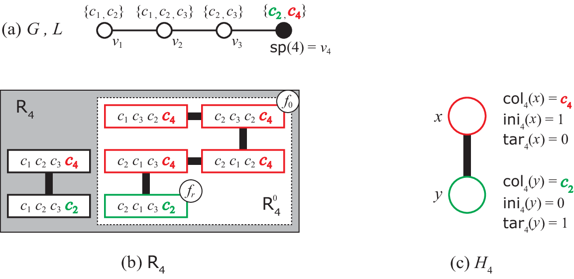
We finally define our dynamic programming table. For each subgraph , , our algorithm keeps track of four information , defined as follows.
- •
The encoding graph of which can be obtained from by contracting each node set in into a single node. (See Figure 5 as an example.) We will refer to an e-node of in order to distinguish it from a node of . (Thus, each node refers to a -list coloring of , and each e-node refers to a set of -list colorings of .) For each e-node , we denote by the set of all nodes in that were contracted into . (Note that we do not compute , but use it only for definitions and proofs.)
- •
The color for each e-node , which is assigned to in common by the nodes (i.e., -list colorings of ) in .
- •
The label for each e-node , such that if , otherwise .
- •
The label for each e-node , such that if , otherwise .
To prove Theorem 4.1, we give a polynomial-time algorithm which computes for each subgraph , , by means of dynamic programming. Then, the problem can be solved as in the following lemma.
Lemma 4
is a yes-instance if and only if the encoding graph contains a node such that .
Proof
Since contains a node such that , we have . Recall that is the encoding graph of which contains the -list coloring of as a node. Since , the lemma clearly follows. ∎
4.2 Algorithm
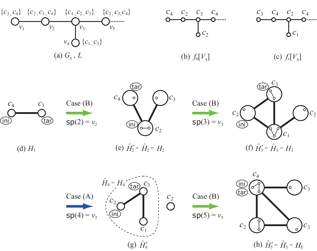
As the initialization, we first consider the case where , that is, we compute . (See Figure 6(d) as an example.) Note that consists of a single vertex , and recall that is a spine vertex of degree one. By Lemma 2 we then have . Therefore, the reconfiguration graph is a complete graph on nodes such that each node corresponds to a -list coloring of which assigns a distinct color to the vertex . Since is complete and contains the node , we have . Furthermore, since all nodes in assign distinct colors in to . Then, for each e-node of corresponding to the set consisting of a single -list coloring of , we set

For , suppose that we have already computed . Then, we compute , as follows.
By Lemma 2 we have in this case; let . Recall that is adjacent with only the spine vertex in . Furthermore, in this case.
Let be the subgraph of obtained by deleting all e-nodes in with . Then, encodes all nodes of that do not assign the color to . Thus, we can extend each -list coloring of encoded in to a -list coloring of such that and for all vertices . Similarly, let be the subgraph of obtained by deleting all e-nodes in with .
We define an encoding graph as and ; and let be the connected component of that contains the e-node such that . For each e-node in , let , and . Then, we have the following lemma.
Lemma 5
For a leaf , .
In this case, notice that in , and hence we need to update according to the color assigned to .
We first define an encoding graph , as follows. For a color , let be the subgraph of obtained by deleting all e-nodes in with . For each connected component in , we add a new e-node to such that ; we denote by the set of all e-nodes in that correspond to . We apply this operation to all colors in . We then add edges to : two e-nodes and in are joined by an edge if and only if .
We now define and for each e-node in , as follows:
and
Let be the connected component of that contains the e-node such that . Then, we have the following lemma.
Lemma 6
For a spine vertex , .
4.3 Running time
We now estimate the running time of our algorithm in Section 4.2. The following is the key lemma for the estimation.
Lemma 7
For each index ,
In particular, , where is the number of vertices in .
By Lemma 7 each encoding graph is of size for each . Therefore, our algorithm clearly runs in polynomial time.
This completes the proof of Theorem 4.1. ∎
5 Concluding Remarks
In this paper, we gave precise analyses of the -list coloring reconfiguration problem with respect to pathwidth: the problem is solvable in polynomial time for graphs with pathwidth one, while it is PSPACE-complete for graphs with pathwidth two.
Very recently, Wrochna [25] gave another proof for the PSPACE-completeness of -list coloring reconfiguration for graphs with pathwidth two. His reduction is constructed from a PSPACE-complete problem, called -Word Reachability.
Acknowledgments
We are grateful to Daichi Fukase and Yuma Tamura for fruitful discussions with them. This work is partially supported by JSPS KAKENHI Grant Numbers 25106504 and 25330003.
References
- [1] Bonamy, M., Johnson, M., Lignos, I., Patel, V., Paulusma, D.: Reconfiguration graphs for vertex colourings of chordal and chordal bipartite graphs. J. Combinatorial Optimization 27, pp. 132–143 (2014)
- [2] Bonamy, M., Bousquet, N.: Recoloring bounded treewidth graphs. Electronic Notes in Discrete Mathematics 44, pp. 257–262 (2013)
- [3] Bonsma, P.: Rerouting shortest paths in planar graphs. Proc. of FSTTCS 2012, pp. 337–349 (2012)
- [4] Bonsma, P.: The complexity of rerouting shortest paths. Theoretical Computer Science 510, pp. 1–12 (2013)
- [5] Bonsma, P., Cereceda, L.: Finding paths between graph colourings: PSPACE-completeness and superpolynomial distances. Theoretical Computer Science 410, pp. 5215–5226 (2009)
- [6] Bonsma, P., Kamiński, M., Wrochna, M.: Reconfiguring independent sets in claw-free graphs. Proc. of SWAT 2014, LNCS 8503, pp. 86–97 (2014)
- [7] Bonsma, P., Mouawad, A.E.: The complexity of bounded length graph recoloring. arXiv:1404.0337 (2014)
- [8] Brandstädt, A., Le, V.B., Spinrad, J.P.: Graph Classes: A Survey. SIAM (1999)
- [9] Cereceda, L.: Mixing Graph Colourings. Ph.D. Thesis, London School of Economics and Political Science (2007)
- [10] Cereceda, L., van den Heuvel, J., Johnson, M.: Finding paths between -colorings. J. Graph Theory 67, pp. 69–82 (2011)
- [11] Gopalan, P., Kolaitis, P.G., Maneva, E.N., Papadimitriou, C.H.: The connectivity of Boolean satisfiability: computational and structural dichotomies. SIAM J. Computing 38, pp. 2330–2355 (2009)
- [12] Hearn, R.A., Demaine, E.D.: PSPACE-completeness of sliding-block puzzles and other problems through the nondeterministic constraint logic model of computation. Theoretical Computer Science 343, pp. 72–96 (2005)
- [13] Ito, T., Demaine, E.D., Harvey, N.J.A., Papadimitriou, C.H., Sideri, M., Uehara, R., Uno, Y.: On the complexity of reconfiguration problems. Theoretical Computer Science 412, pp. 1054–1065 (2011)
- [14] Ito, T., Kamiński, M., Demaine, E.D.: Reconfiguration of list edge-colorings in a graph. Discrete Applied Mathematics 160, pp. 2199–2207 (2012)
- [15] Ito, T., Kawamura, K., Ono, H., Zhou, X.: Reconfiguration of list -labelings in a graph. To appear in Theoretical Computer Science. DOI: 10.1016/j.tcs.2014.04.011
- [16] Ito, T., Kawamura, K., Zhou, X.: An improved sufficient condition for reconfiguration of list edge-colorings in a tree. IEICE Trans. on Information and Systems E95-D, pp. 737–745 (2012)
- [17] Jansen, K., Scheffler, P.: Generalized coloring for tree-like graphs. Discrete Applied Mathematics 75, pp. 135–155 (1997)
- [18] Johnson, M., Kratsch, D., Kratsch, S., Patel, V., Paulusma, D.: Colouring reconfiguration is fixed-parameter tractable. arXiv:1403.6347 (2014)
- [19] Kamiński, M., Medvedev, P., Milani, M.: Shortest paths between shortest paths. Theoretical Computer Science 412, pp. 5205–5210 (2011)
- [20] Kamiński, M., Medvedev, P., Milani, M.: Complexity of independent set reconfigurability problems. Theoretical Computer Science 439, pp. 9–15 (2012)
- [21] Makino, K., Tamaki, S., Yamamoto, M.: An exact algorithm for the Boolean connectivity problem for -CNF. Theoretical Computer Science Theor. Comp. Sci. 412, pp. 4613–4618 (2011)
- [22] Mouawad, A.E., Nishimura, N., Raman, V., Simjour, N., Suzuki, A.: On the parameterized complexity of reconfiguration problems. IPEC 2013, pp. 281–294 (2013)
- [23] Proskurowski, A., Telle, J.A.: Classes of graphs with restricted interval models. Discrete Mathematics & Theoretical Computer Science 3, pp. 167–176 (1999)
- [24] Robertson, N., Seymour, P.: Graph minors. I. Excluding a forest. J. Combinatorial Theory, Series B, 35, pp. 39–61 (1983)
- [25] Wrochna, M.: Reconfiguration in bounded bandwidth and treedepth. arXiv:1405.0847 (2014)
Appendix 0.A Proofs Omitted from Section 4
We first introduce some notation.
For , let be any node (i.e., a -list coloring of ) in the reconfiguration graph . Recall that the vertex is adjacent with only the spine vertex in . Let be any color in . Then, we say that can be extended by to a -list coloring of such that and for all vertices ; we simply denote such an extension by . Note that is a node in .
For any e-node in the encoding graph of , recall that is the set of all nodes in that were contracted into . For a color , let , that is, is the set of nodes in that are extended by from nodes in .
0.A.1 Proof of Lemma 5
In this subsection, we prove Lemma 5. Therefore, suppose that we have already computed for , and assume that and .
We first prove that holds, as in the following lemma.
Lemma 8
Let be any e-node in . Then, there exists an e-node in such that .
Proof
Let be any node in . Then, by Lemma 3 the node is contained in , and hence there exists an e-node in such that . Notice that, since , we have . Thus, the e-node is contained in , too. Therefore, we prove that .
Let be any node in . Then, , and hence contains a path such that , and for all . Thus, we can obtain a path in which the spine vertex always receives the same color ; note that may hold if is recolored, but we can simply drop in such a case. Since for the case where , we have . Therefore, . Since represents the color assigned to and is adjacent with in , the color is clearly contained in . We thus have .
Let be any node in such that for some node in and . Since and , we have and hence contains a path such that , and for all . Since and , the sequence is a path in . If , we add one more adjacent node to the last. Since and , we thus have and hence . ∎
By Lemma 8 we may identify each e-node in with the corresponding e-node in .
We then prove the following lemma.
Lemma 9
Let and be two e-nodes in , and let and be two e-nodes in corresponding to and , respectively. Then, if and only if .
Proof
We first prove the only-if-part. Suppose that ; it is symmetric for the other case where . Then, there exist two adjacent nodes and such that and . Therefore, by Lemma 8 we have and . Note that, since , we know that only the spine vertex is recolored between and . Thus, and are adjacent in , and hence we have .
We then prove the if-part. Since , there exist two adjacent nodes and in . Since , only the spine vertex is recolored between and , and hence . Therefore, and are adjacent. We assume that without loss of generality. Then, since and are adjacent, and . By Lemma 8 we have ; this implies that . Similarly, . Since and are adjacent, . Furthermore, since and , we have . Therefore, . ∎
We now prove the following lemma.
Lemma 10
.
Proof
Recall that consists of a single connected component which contains the e-node such that . Consider the set of all e-nodes in that correspond to the e-nodes in . By Lemma 9 the e-node set forms a connected subgraph of a single connected component in . Furthermore, by Lemma 8 the component in contains the e-node such that ; by the construction, is contained in . We thus have .
Therefore, to show , by Lemma 9 it suffices to prove that there exists no edge which joins two e-nodes and . Suppose for a contradiction that there exists such an edge . By the construction, ; we may assume that without loss of generality. Then, there exist two adjacent nodes and such that and . Therefore and can be extended by , and and are adjacent in . By Lemma 8 we then have ; this contradicts the assumption that . ∎
Finally, we show the following lemma.
Lemma 11
, and .
Proof
Recall that if . Then, the lemma follows immediately from Lemma 8. ∎
This completes the proof of Lemma 5.
0.A.2 Proof of Lemma 6
In this subsection, we prove Lemma 6. Therefore, suppose that we have already computed for , and assume that .
We first prove that holds, as in the following lemma.
Lemma 12
Let be any e-node in with . Then, there exists exactly one connected component in such that .
Proof
Let be any node in . Then, by Lemma 3 the node is contained in , and hence there exists an e-node in such that . Since and is adjacent with , the assumption implies that and hence . Therefore, we have , and hence has exactly one connected component that contains . We thus prove that for the connected component .
Let be any node in . Then, and hence it suffices to show that contains an e-node such that . Since , there exists a path in such that , and for all . Since is adjacent with , holds for all . Therefore, there exists a connected component in such that the path is contained in . Because and , we have . Thus, contains an e-node such that . Then, we have .
Conversely, let be any node in . Since is connected, the subgraph of induced by is connected, too. Then, the induced subgraph contains a path such that and . Furthermore, since is a connected component in , we know that for all nodes , . Therefore, we can extend each node by , and obtain a path . Since and , we thus have . Since , we have . ∎
For each e-node , let be the connected component in which satisfies Lemma 12. Then, we can identify the e-node in with the e-node in such that .
We then prove the following lemma.
Lemma 13
Let and be two e-nodes in , and let and be two e-nodes in corresponding to and , respectively. Then, if and only if .
Proof
We first prove the only-if-part. Suppose that the set contains an e-node in . Choose an arbitrary node , then two nodes and are adjacent in . Thus, .
We then prove the if-part. Suppose that , then there exist two adjacent nodes and in . Since and are adjacent and , we know that . By Lemma 12, there exists an e-node such that . Similarly, there exists an e-node such that . Since , we have . Therefore, . ∎
We now prove the following lemma.
Lemma 14
and .
Proof
We prove only ; it is similar to prove .
Let be any e-node in such that . Then, , and holds. By Lemma 12 there exists an e-node such that and . Since , we thus have .
Conversely, let be any e-node in such that . Then, contains an e-node such that and . Note that is in , and . By Lemma 12 we thus have and hence . ∎
Finally, we show following lemma.
Lemma 15
.
Proof
Recall that consists of a single connected component which contains the e-node such that . By Lemma 13 is contained in one connected component of as a subgraph, and the connected component contains an e-node such that . By Lemma 14 we have , and hence the connected component is indeed . We thus have .
Therefore, to show , by Lemma 13 it suffices to prove that there exists no edge which joins two e-nodes and . Suppose for a contradiction that there exists such an edge . Then, the set contains an e-node . Choose an arbitrary node , then two nodes and are adjacent in . Then, . By Lemma 12 the corresponding e-node should be contained in ; this contradicts the assumption that . ∎
This completes the proof of Lemma 6.
0.A.3 Proof of Lemma 7
In this subsection, we prove Lemma 7. Since holds, it suffices to prove the following inequality: for each index ,
| (3) |
Consider the case where is a leaf. Then, , and hence Eq. (3) clearly holds. In the remainder of this subsection, we thus consider the case where is a spine vertex.
For a graph , we denote by the number of connected components in . For a connected graph , that is, , we denote by any spanning tree of . Since , we clearly have the following proposition.
Proposition 1
Let be a connected graph, and let be any vertex subset of . Then, holds.
We now apply Case (B) of our algorithm to any spanning tree of , instead of applying the operation to . Let be the obtained encoding graph, instead of . Then, we have the following lemma.
Lemma 16
.
Proof
For each color , let be the subgraph of obtained by deleting all e-nodes in with . Then,
and
| (4) |
By Proposition 1 we have for each color , and hence . ∎
We finally show the following lemma, which verifies Eq. (3) and hence completes the proof of Lemma 7.
Lemma 17
If is a spine vertex, then .
Proof
We then consider the case where . Recall that is a spanning tree of , and hence . For each color , let . For each vertex , we denote by the degree of in . Then, by deleting from , the number of connected components in the resulting graph is increased by . We thus have
| (5) | |||||
By Lemma 16 and Eq. (4) we have
Therefore, by Eq. (5) we have
| (6) | |||||
Since is a tree, . Furthermore, recall that is a spanning tree of , and hence . By Eq. (6) we thus have . By Lemma 2 we have , and hence
as required. ∎