Transverse Spin and Classical Gluon Fields: Combining Two Perspectives on Hadronic Structure
Abstract
In recent decades, the spin and transverse momentum of quarks and gluons were found to play integral roles in the structure of the nucleon. Simultaneously, the onset of gluon saturation in hadrons and nuclei at high energies was predicted to result in a new state of matter dominated by classical gluon fields. Understanding both of these contributions to hadronic structure is essential for current and future collider phenomenology. In this Dissertation, we study the combined effects of transverse spin and gluon saturation using the Glauber-Gribov-Mueller / McLerran-Venugopalan model of a heavy nucleus in the quasi-classical approximation. We investigate the use of a transversely-polarized projectile as a probe of the saturated gluon fields in the nucleus, finding that the transverse spin asymmetry of produced particles couples to the component of the gluon fields which is antisymmetric under both time reversal and charge conjugation. We also analyze the effects of saturation on the transverse spin asymmetry (Sivers function) of quarks within the wave function of the nucleus, finding that gluon saturation preferentially generates the asymmetry through the orbital angular momentum of the nucleons, together with nuclear shadowing.
Yuri Kovchegov \degreeDoctor of Philosophy \memberEric Braaten \memberMichael Lisa \memberSamir Mathur \authordegreesM.S. , B.S. , B.A. \graduationyear2014 \unitGraduate Program in Physics
To all the teachers, professors, and mentors who have invested so much of themselves and their passion in me and my future. I can see further than I ever thought possible because I stand on the shoulders of giants.
Acknowledgements.
First and foremost, I owe great thanks to my advisor Yuri Kovchegov. Your amazing ability to explain both the technical details and the underlying physics principles makes you a phenomenal physicist, teacher, and advisor. You have been equally willing to help me wrestle with the big questions and to get your hands dirty helping me search for my minus signs and factors of 2, and you have somehow always found time for me in your busy schedule. Learning a new field of study together with you has taught me by example what it means to be a physicist. To James and Veronica and Logan, to Jer and Kristie and Chloe, to Aidan, and especially to my love Jesse – I cannot thank you enough for keeping me sane, for giving me perspective, and for believing in me when I have had nothing left but doubts. Your strength and love make me a whole person and fill my life with meaning and purpose. To Adam and David and Alexis, and to all my fellow karateka – thank you beyond measure for pushing me, for challenging me, for accepting and respecting me, for inspiring and competing with me, for not hesitating to throw the punch when I leave my guard down. You help me to hold myself to a higher standard and to continually seek perfection of character. And to Mom and Dad – thank you for everything. For fostering my curiosity and my love of learning. For teaching me division with sunflower seeds. For pushing me to work harder in school when I just wanted to play video games. For teaching me tolerance and responsibility. For celebrating my successes and forgiving my failures. For loving and accepting me and respecting me as an adult, and for always believing in me. I love you from the bottom of my heart.August 5, 1984Born—Lexington, VA \dateitemMay, 2002Chesterfield County Mathematics and Science High School at Clover Hill, Midlothian, VA \dateitemMay, 2006B.S. Physics, B.A. Spanish, Virginia Commonwealth University, Richmond, VA \dateitemAugust, 2007M.S. Physics, Virginia Commonwealth University, Richmond, VA \dateitem2007 - 2008William A. Fowler Graduate Fellow in Physics, The Ohio State University, Columbus, OH \dateitem2007 - 2008 ; 2010 - presentSusan L. Huntington Distinguished University Fellow, The Ohio State University, Columbus, OH
Y. V. Kovchegov and M. D. Sievert, “A New Mechanism for Generating a Single Transverse Spin Asymmetry”, Phys. Rev. D86, 034028 (2012) \pubitemY. V. Kovchegov and M. D. Sievert, “Single Spin Asymmetry in High Energy QCD”, Int. J. Mod. Phys. Conf. Ser. 20, 177 (2012) \pubitemM. D. Sievert, “A New Mechanism for Generating a Single Transverse Spin Asymmetry”, Nucl. Phys. A 904-905, 833c (2013) \pubitemS. J. Brodsky, D. S. Hwang, Y. V. Kovchegov, I. Schmidt, and M. D. Sievert, “Single-Spin Asymmetries in Semi-Inclusive Deep Inelastic Scattering and Drell-Yan Processes”, Phys. Rev. D88 014032 (2013) \pubitemM. D. Sievert, “Single-Spin Asymmetries in Semi-Inclusive Deep Inelastic Scattering and Drell-Yan Processes”, Int. J. Mod. Phys. Conf. Ser. 25 1460015 (2014) \pubitemY. V. Kovchegov and M. D. Sievert, “Sivers Function in the Quasi-Classical Approximation”, Phys. Rev. D89, 054035 (2014)
Physics {studieslist} \studyitemGluon saturation in high-energy QCDYuri V. Kovchegov
This research is sponsored in part by the U.S. Department of Energy under Grant No. DE-SC0004286.
Chapter 1 Overview
Since the proton was first discovered a century ago, the quest to understand its quantum structure has revealed layer upon layer of new mysteries. Each successive breakthrough we make in resolving its subcomponents and their properties opens the door to new puzzles which fundamentally challenge our understanding of hadronic physics. The quark model [4, 5, 6] organized the baffling zoo of hadronic particles in the proton’s family tree into a logical “periodic table,” but the absence of free quarks in nature thwarted early attempts to formulate them into a quantum theory. The advent of the theory of quantum chromodynamics [7, 8] with the remarkable property of asymptotic freedom bridged this gap, reconciling long-standing challenges to the validity of quantum field theory itself, but it also implied a fundamental disconnect between the elementary quarks and gluons of the theory and the hadronic degrees of freedom seen in nature. Each step in the development of our understanding has revealed another hidden layer of structure and complexity, driving still further advances in both theory and experiment.
In this Dissertation, we present an analysis of two such layers of structure which have been developed largely in parallel over the last 30 years, together with our recent work to understand their interconnection. The first of these layers involves the complex spin-orbit and spin-spin coupling mechanisms that translate the spin of hadrons like the nucleon (proton or neutron) into the spins and orbital motion of its quark and gluon constituents. This paradigm has been driven largely by past and current experiments which continue to demonstrate the importance of spin and transverse momentum to our understanding of hadronic structure. The second involves the coherent nonlinear interactions that occur in high-energy scattering when the density of quarks and gluons inside the hadron is large. This saturation paradigm has been driven largely by theoretical considerations which demand that new physical processes take over at high energies and densities in order to preserve the internal consistency of the theory. Our efforts to combine these two paradigms have resulted in new insights, both into how spin physics can be used as a probe of saturation, as well as how saturation mechanisms can mediate the exchange of spin and transverse momentum. These insights open the door to future work extending the interplay of spin and saturation, and the analysis presented here represents only a small portion of the active frontiers of research into hadronic structure.
1.1 The Evolving Picture of the Nucleon
1.1.1 Quark and Gluon Degrees of Freedom
The quark model proposed by Gell-Mann and Zweig in 1964 [4, 5, 6] explained the relationship between the proton, neutron, and other hadrons based on the charges of their constituent quarks. In this picture, the proton is composed of two “up” quarks with electric charge and one “down” quark with electric charge , where is the magnitude of the electron charge. Similarly, the neutron is composed of two “down” quarks and one “up” quark. Each constituent quark would have a mass of around of the proton mass, on the order of . Since the postulated quarks are spin- fermions, they can also simply account for the total spin of the nucleon if two constituent quarks have their spins aligned parallel to the nucleon and one antiparallel, as illustrated in Fig. 1.1. While successful at capturing the relationships between the masses and charges of the hadrons, the quark model was not a quantum theory and did not describe the interactions of the quarks which bind them into hadrons.

The key to determining the properties of the quark interactions came from the SLAC-MIT experiment [9, 10] in 1968, which studied the deep inelastic scattering of high-energy electrons on hadronic targets. The hard electromagnetic scattering was consistent with the nucleon being composed of a number of pointlike constituents collectively called partons [11]. The scaling properties observed in the SLAC-MIT experiment [12, 13] confirmed that the charged partons are spin- fermions and suggested that their interactions over short times and distances are weak, but strong enough over long times and distances to bind them together into hadrons. These properties are in stark contrast to those of quantum electrodynamics (QED), whose quantum self-interactions become strongest at short distances.
The insight that the interaction of quarks must possess asymptotic freedom at short distances led to the development in 1973 of a full-fledged quantum field theory known as quantum chromodynamics (QCD) [7, 8]. Like its close cousin quantum electrodynamics, QCD is a quantization of a classical theory of charges and fields, but whereas QED quantizes the linear Maxwell equations, QCD quantizes the highly-nonlinear Yang-Mills equations [14]. The Yang-Mills equations are structurally similar to the Maxwell equations, with one essential difference: the field itself is charged and can act as a source for further radiation. In the quantum analog, this means that the gluon fields of QCD interact with themselves and each other, unlike the photons of QED. This additional self-interaction is essential to generating asymptotic freedom, and the rigorous development of its quantum origins from the QCD Lagrangian helped put quantum field theory itself on a firm footing. The intrinsic breakdown of QED and similar theories at short distances (or high energies) had cast fundamental doubt on the validity of quantum field theory itself as a framework for quantum mechanics [15, 16], but the asymptotic freedom embodied by QCD resolved this crisis by providing a theory which is “UV complete” – self-consistent up to arbitrarily high energies.
The price of asymptotic freedom is that the interactions between quarks and gluons become strongest at low energies, such as those relevant for the calculation of the nucleon wave function. In principle this information is encoded in the QCD Lagrangian, but because of the strong coupling it cannot be calculated perturbatively from the fundamental theory. This reflects the physics of quark confinement: while quarks and gluons are the relevant degrees of freedom at short distances and high energies, the emergent degrees of freedom at long distances and low energies are their bound states: nucleons, pions, and the whole zoo of hadronic particles. When the wave function of the nucleon is probed by a high-energy projectile as in deep inelastic scattering, the short-distance interactions with the quarks and gluons can be calculated perturbatively, but the observables are always contaminated by nonperturbative, incalculable low-energy quantities. The bridge between the perturbative and nonperturbative elements of QCD is provided in the form of factorization theorems (see, e.g. [17, 18, 19, 20]) which show that the distribution of quarks and gluons within a hadron can be measured with one process and used predictively in another.

The picture of the nucleon changes depending on the kinematics of the scattering process used to probe its wave function; in particular, the scaling variable denoted describes the fraction of the nucleon’s longitudinal momentum carried by the partons (see Chapter 2). This picture is visualized in Fig. 1.2. At large , the nucleon appears to be composed of three valence quarks sharing the nucleon’s momentum, as in the quark model. As decreases, the scattering probe becomes less sensitive to the valence quarks and more sensitive to the partons produced by radiation, which tend to share smaller fractions of the nucleon momentum among a larger number of particles. At very small , the nucleon wave function is dominated by a large number of gluons, each sharing a very small fraction of the total momentum. This picture of the nucleon as resolved into a collinear beam of quarks and gluons [12, 11] was immensely successful in explaining the structure observed in deep inelastic scattering experiments over a wide range of kinematics [21, 22, 23, 24, 25].
1.1.2 Spin and Transverse Momentum
This simple one-dimensional picture of nucleon structure was shattered by groundbreaking experiments that revealed a far more complex role played by spin and partonic transverse momentum. The European Muon Collaboration performed measurements in 1988 on longitudinally-polarized protons that measured the spin contribution carried by the quarks; in striking contradiction to the naive expectation shown in Figs. 1.1 and 1.2, they found that only “ of the proton spin is carried by the spin of the quarks” [26]. This shocking result came to be known as the proton spin crisis, and their conclusion that “the remaining spin must be carried by gluons or orbital angular momentum” inaugurated a worldwide effort to find the missing angular momentum which continues to this day.
In general, the spin of the nucleon can be decomposed into a part coming from the net polarization of the spin- quarks, a part from the net polarization of the spin-1 gluons, and the orbital angular momentum and of quarks and gluons, respectively [27]:
| (1.1) |
Modern determinations [28] of the quark spin estimate the contribution at about , corresponding to of the proton spin, and very recent measurements [29, 30] of the gluon polarization find a contribution of about , corresponding to of the proton spin. Although these values are not very precisely determined, they still leave significant room for the contribution of the angular momentum of quarks and gluons coming from their transverse motion.
A similarly dramatic revelation occurred with regard to the role of transverse polarization. An expectation dating as far back as Feynman [31] predicted that transverse polarization effects are universally suppressed at high energies (see also [32] and the discussion in [20]). But in 1991 when the E581/E704 Collaborations at Fermi National Accelerator Laboratory (FNAL) measured the single transverse spin asymmetry (STSA) produced in collisions of transversely-polarized protons, they found strikingly large asymmetries of up to 30-40% [33, 1, 34, 35, 36, 37]. More recently, the PHENIX, STAR, and BRAHMS collaborations at the Relativistic Heavy Ion Collider (RHIC) have studied transverse spin asymmetries at a higher energy and over a wide kinematic range [38, 39, 40, 41]. The data they have presented [38, 39, 40] confirmed and extended the Fermilab results, and also indicated a non-monotonic dependence of STSA on the transverse momentum of the produced hadron [2, 42]. Some of these plots are reproduced in Fig. 1.3; for a useful review of STSA physics see [43].

 |
The implications of these experiments have led to a considerable broadening of our picture of nucleon structure. The nucleon’s “spin budget” (Fig. 1.4) is distributed among the polarizations and transverse orbital motion of quarks and gluons, which can manifest themselves in a number of spin and momentum correlations that are observable in hadronic collisions. The generalization to a three-dimensional picture of nucleon structure, including transverse momentum and its correlations with the nucleon and parton spins is made possible by more inclusive versions of factorization theorems (see, e.g. [44, 45, 46, 47, 20]). While this formalism brings the intricate spin-orbit and spin-spin correlations in the nucleon within reach of theory and experiment, it also opens the door to still further challenges and opportunities. The universality of the parton distributions, for example, is lost by the inclusion of transverse momentum [48], and in some processes the properties of the target and projectile seem to be entangled so that they cannot even be separately defined [49, 50]. As with the other historic advances in our understanding of nucleon structure, the inclusion of spin and transverse momentum answers our questions with still more questions. We discuss the spin and transverse momentum paradigm of hadronic structure in detail in Chapter 2.

1.1.3 Gluon Saturation
While the distributions of quarks and gluons within the nucleon are fundamentally low-energy quantities that are not perturbatively calculable in QCD, the manner in which these distributions evolve with external parameters are. These quantum evolution equations describe how QCD radiative processes modify the distribution of partons, such as by the collinear emission of gluons or pair-production of quarks [51, 52, 53]. The momentum fraction of partons resolved in a hadronic collision is kinematically related to the center-of-mass energy at which the collision occurs. As the energy is increased, is decreased, and the nucleon structure becomes dominated more and more by gluons as shown in the right panel of Fig. 1.2.

The origin of these additional gluons is through the quantum evolution [54, 55] of the pre-existing partons, which radiate gluons through bremsstrahlung when the energy is increased (Fig. 1.5, open circles). The effect of this bremsstrahlung is to increase the density of gluons in the nucleon as a function of the collision energy. But as the energy is increased further, these new gluons themselves undergo bremsstrahlung, increasing the gluon density even faster. The result of this rapid proliferation of gluons is to make the nucleon more and more opaque to a high-energy projectile as the energy continues to increase. If the successive gluon radiation were to continue unabated, it would lead to scattering probabilities greater than at high energies, which would violate the fundamental principle of unitarity in quantum mechanics [56, 57, 58].
Unitarity is a non-negotiable element of quantum field theory, and its preservation demands that the structure of the nucleon at high energies must be very different from the low-energy structure that gives rise to this exploding gluon density. At sufficiently high density the spatial distribution of gluons begins to overlap, leaving no available space for additional independent bremsstrahlung. When this happens, the nonlinear interactions between the radiated gluons become important, including their recombination through gluon fusion (Fig. 1.5, solid circles). Gluon fusion tends to decrease the gluon density and so competes with the increase due to bremsstrahlung; when these effects become comparable, the gluon density saturates and cuts off the growth with energy [59, 60]. The result is that the structure of the nucleon at very high energies is driven overwhelmingly by gluon fields with high densities and occupation numbers; in this saturation regime the dominant degrees of freedom are the classical gluon fields obtained from the Yang-Mills equations [61].
The onset of saturation at high densities, although not yet observed unambiguously in experiment, is necessary for the consistency of nucleon structure with the unitarity of quantum field theory. When these high-density effects are included into the small- quantum evolution equations, the resulting nonlinear evolution explicitly preserves unitarity [62, 63, 64, 65, 66, 67, 68]. The same limit of high gluon densities can also be obtained in a different physical system: a heavy nucleus with a large number of nucleons [69, 70, 71, 72, 73, 74, 75, 76, 77]. This approach provides a much more direct route to obtaining the physical properties of the saturation regime, without the need to solve the complicated small- quantum evolution equations. We discuss the onset of saturation in a heavy nucleus and the emergence of classical gluon fields in detail in Chapter 3.
1.2 Organization of this Document
This document is structured as follows. In Chapter 2 we introduce the formalism for describing the transverse-momentum-dependent distributions of quarks and gluons in a hadron, in the context of deep inelastic scattering. After reviewing the foundational knowledge in the field, we present original work analyzing one of these transverse-momentum-dependent parton distribution functions in detail in Sec. 2.3. In Chapter 3 we lay out the saturation formalism relevant for the resummation of high-density effects at high energies, emphasizing the role of multiple scattering and the emergence of classical gluon fields as the relevant degrees of freedom. Then we present original work analyzing the interplay between these paradigms in two ways, demonstrating how each provides the tools to acquire new understanding of the other. In Chapter 4 we show how transverse spin can be used as a tool to study novel aspects of the saturation regime by accessing a different component of the dense gluon fields. Then in Chapter 5 we use the saturation formalism to elucidate a new relationship between the transverse-momentum-dependent quark distributions and their orbital angular momentum. We conclude with a brief outlook in Chapter 6 which summarizes the main results presented here and proposes the next logical steps which can be taken to extend them.
1.2.1 Notation and Conventions
Wherever possible, we choose our conventions to correspond with those of [78]. As is standard, we work in natural units in which .
We work with the QCD Lagrangian in the form
| (1.2) | ||||
where denotes the quark flavor, are color indices in the fundamental representation of the gauge group, are color indices in the adjoint representation of the gauge group, and are the structure constants. The gauge group of QCD is with generators in the fundamental representation related to the Gell-Mann matrices by ; however, it is convenient to work in the more general gauge group with the number of colors. This makes the group-theoretical structure of the formulas more explicit and allows us to take advantage of ’t Hooft’s large- limit [79] in Chapter 4. The sum of the squares of the generators of the group is known as the quadratic Casimir invariant [80]. In the fundamental representation this is given by
| (1.3) |
which gives for . The quadratic Casimir in the adjoint representation is just equal to the number of colors, .

In high-energy interactions with particles traveling very close to the speed of light, it is convenient to work in light-cone coordinates as in Fig. 1.6 which are linear combinations of and . We choose the normalization of the coordinates and the corresponding metric tensor to be
| (1.4) | ||||
where vectors which are underlined represent transverse vectors in the plane. Thus we label the components of a 4-vector as
| (1.5) | ||||
and use the subscript to denote the component of a transverse vector. For the magnitude of a transverse vector, we use the subscript , as in
| (1.6) | ||||
The antisymmetric (“cross”) product of two transverse vectors is given in terms of the two-dimensional antisymmetric Levi-Civita tensor as
| (1.7) |
The normalization of the light-cone coordinates and the corresponding metric in (1.4) is not universal; often one uses coordinates normalized by so that there are no factors of appearing in the metric. At times the factors of 2 in our convention will be a convenience and at other times an inconvenience.
For brevity’s sake, in many of the formulas we will abbreviate the notation for multi-dimensional integration. For integration over a transverse variable we use the notation which is commonplace, and sometimes we wish to integrate over transverse variables and one light-cone coordinate, for which we will use the notation
| (1.8) | ||||
and similarly for the arguments of Dirac delta functions like or .
A common variable in high-energy collisions is the rapidity of an on-shell particle with momentum , denoted
| (1.9) |
where we have made use of the on-shell condition . In terms of rapidity, the invariant differential cross-section is written as
| (1.10) |
When identifying the power-counting in large kinematic quantities such as the center-of-mass energy squared , we will often compare them to smaller quantities such as masses or transverse momenta, which we generically assume to be of the order of the masses unless otherwise specified. We denote the order of such quantities generically as , as in “.”
Finally, in some cases we will perform calculations using ordinary Feynman perturbation theory through the use of Feynman diagrams. In others, particularly in the high-energy limit, it is more convenient to calculate observables through the use of light-cone perturbation theory (LCPT). LCPT corresponds to time-ordered perturbation theory in the ordinary sense, but with the light-cone coordinate playing the role of time (for a particle moving along the axis with high energy). The natural ordering of high-energy processes in makes this a useful tool, and we use the conventions of [78] unless otherwise specified.
Chapter 2 The Spin and Transverse Momentum Paradigm of Hadronic Structure
The most natural way to measure the structure of the nucleon is through its interaction with an electromagnetic probe. If an incident electron scatters off the nucleon by exchanging a spacelike virtual photon, the injected momentum may cause the nucleon to break up inelastically into a multi-hadron final state: . The uncertainty principle suggests that the larger the momentum transfer, the smaller the distance scales on which the charge distribution is measured. Thus, for the case of deep inelastic scattering (DIS) when the photon virtuality is large, the electron interacts with the charged sub-components of the nucleon. In this way, deep inelastic scattering gives a direct window into the substructure of the nucleon, and it played a key role in the historical establishment of QCD as the fundamental theory of the strong nuclear force (see, e.g. [7, 8, 81] and [82] for a review).
The simplest application of this idea is in the form of the parton model [31, 83], in which the virtual photon is assumed to interact with a single charged sub-component of the nucleon. These pointlike constituents are collectively referred to as “partons,” and it is possible to determine whether they are bosons or fermions from the form of the resulting cross-section [13]. In this way, “partons” were identified as charged fermions (quarks) and their associated QCD gauge field (gluons).
The parton model reduces the process of deep inelastic scattering to a fixed, short-distance electromagnetic vertex [84, 85] that effectively “measures” the distribution of quarks within the nucleon wave function. This allows the nucleon structure to be parameterized in terms of parton distribution functions (PDF’s) which resolve the nucleon into a collinear beam of quarks and gluons. Although significantly modified by QCD corrections, this essential concept survives in the form of collinear factorization (see, e.g. [17, 18, 86] and the textbooks [19, 20]). Once suitably generalized, these parton distribution functions can be shown to be intrinsic, universal properties of the nucleon which can be measured in one experiment and then used predictively in another. These theoretical cornerstones form the basis of the collinear paradigm of hadronic structure, which has been immensely successful in describing experimental data over many orders of magnitude in [21, 22, 23, 24, 25].
A series of revolutionary experiments in the early 90’s (see [26, 33, 1, 34, 35], among others) revealed the surprising importance of spin and transverse-momentum dynamics, which are not captured in the collinear paradigm. Differential observables that describe the azimuthal distribution of produced hadrons provide another external “lever” to parameterize the nucleon’s substructure. One such differential observable is semi-inclusive deep inelastic scattering (SIDIS), in which both the scattered lepton and one final-state hadron are tagged: . Like the fully-inclusive case, SIDIS couples to parton distribution functions, but now with the transverse momentum of the active parton accessible through the momentum of the tagged hadron . These transverse-momentum-dependent parton distribution functions (TMD’s) are capable of resolving both the transverse and longitudinal structure of the nucleon, adding another dimension to the parameter space of parton distributions. As with the collinear case, the naive parton model is heavily modified by QCD corrections into the modern form of TMD factorization (see, e.g. [44, 45, 46, 47, 20]) .
The inclusion of dependence on the nucleon spin, parton spin, and parton transverse momentum permits a wealth of new spin-momentum correlations in the SIDIS cross-section and in the TMD’s. The potential for such nontrivial spin-orbit and spin-spin coupling in the nucleon mirrors the role of the fine and hyperfine structure in atomic physics. Among these spin correlations, transverse spin plays a distinct role from that of longitudinal spin (helicity) because it introduces a preferred direction in the transverse plane. For a singly-polarized process such as SIDIS on a polarized nucleon, rotational invariance uniquely couples the transverse spin direction of the nucleon to the transverse momentum direction of the produced hadron, resulting in a single transverse spin asymmetry (STSA) of the detected hadrons. Furthermore, the discrete symmetries of QCD: charge-conjugation, parity, and time-reversal (, , and ), strongly constrain the form of spin correlations such as STSA - and the partonic mechanisms that can generate them. The combination of parity and time reversal (sometimes called “naive time reversal”) plays a particularly important role in the origin of STSA because this symmetry operation flips the direction of the transverse spin, while leaving the momenta of the colliding particles unchanged; thus STSA is odd under .
The partonic analog of STSA is a TMD called the Sivers function [87], a correlation between the transverse spin of the nucleon and the transverse orbital momentum of its partons. Like STSA, the Sivers function is by definition odd under “naive time reversal”; but unlike STSA, the Sivers function is interpreted as an intrinsic property of the nucleon. Since the nucleon wave function is an eigenstate of the QCD Hamiltonian, it must be -even, so it is natural to expect that the Sivers function is identically zero. However, this expectation is wrong because of an essential difference between the collinear and transverse-momentum paradigms; while the collinear PDF’s can be simply written as densities of partons, in TMD’s the parton densities are fundamentally entangled with initial- and final-state interactions. The nontrivial role played by initial- and final-state interactions permits a nonzero Sivers function, and time reversal further implies that the Sivers function measured in processes with final-state interactions is equal in magnitude and opposite in sign from processes with initial-state interactions [48]. When TMD factorization holds, this gives rise to the prediction of an exact sign reversal between the Sivers functions in SIDIS and its mirror image: the Drell-Yan process. The diagrammatic mechanism of this sign reversal can be examined within the context of a simple model for the nucleon [88]. Although the model verifies the predicted sign flip at leading order in the hard scale , it suggests that violations may occur at subleading orders. This model calculation also motivates a physical interpretation of the sign-flip relation in terms of the “QCD lensing” of quarks due to initial- or final-state interactions [89, 90].
2.1 Spin- and Momentum-Dependent Observables
2.1.1 Inclusive and Semi-Inclusive Deep Inelastic Scattering
Because of asymptotic freedom and quark confinement [7, 8], one of the most direct ways to experimentally probe the quark and gluon degrees of freedom is through deep inelastic scattering (DIS). In this process, a high energy lepton, which we take here to be an electron, scatters off a nucleon by exchanging a spacelike virtual photon . The deep inelastic regime occurs when the magnitude of the momentum transfer is large; then the injected hard momentum scatters perturbatively off the wave function of the nucleon. Experimentally, measuring the recoil of the electron fixes the kinematics of the scattering, and one may consider the inclusive DIS process containing any final hadronic state or the semi-inclusive DIS process in which one final-state hadronic particle is tagged . The kinematics of DIS are illustrated in Fig. 2.1.

Two conventional choices of Lorentz invariants used to characterize the kinematics of DIS are the photon’s virtuality and the Bjorken variable :
| (2.1) | |||||
| (2.2) |
We will work in the Bjorken limit of the kinematics, in which the virtuality is large compared to the typical scale of the nucleon and is held fixed and . The total invariant mass of the hadronic final state is equal to the photon/nucleon center-of-mass energy ; since this quantity is positive-definite, we have
| (2.3) |
which gives the kinematic range of as in the Bjorken limit.
The emission and propagation of the virtual photon can be expressed using perturbative QED, and, without knowing anything about the structure of the nucleon, we can express its interaction with the virtual photon as a transition matrix element of the electromagnetic current:
| (2.4) |
Here is the momentum of the outgoing electron, and the electromagnetic current of a system of quarks with various flavors is
| (2.5) |
where is the electric charge of quark flavor in units of the electron charge , and a sum over such flavors is implied.
By squaring the amplitude (2.4) and including the associated flux factors and phase-space integrals, we can compute the invariant cross-section in the ordinary way [91, 78], obtaining the standard result
| (2.6) |
where the leptonic tensor for an unpolarized lepton is
| (2.7) |
and the hadronic tensor expresses the interaction with the nucleon in terms of a current-current correlation function:
| (2.8) | ||||
When the photon virtuality is large, the photon resolves an individual parton in the nucleon wave function as shown in Fig. 2.2. If we write the state as the product of an active quark with momentum and an arbitrary state containing the other nucleon remnants, the parton model corresponds to the interaction of the virtual photon with just the quark line.

To proceed from here, it is useful to specify a frame for the process in which to work out the kinematics. Let us for the moment work in the photon-nucleon center-of-mass frame, in which
| (2.9) | ||||
Momentum conservation, together with the on-shell conditions, fix the values of in terms of and various constants:
| (2.10) | ||||
The large (negative) light-cone plus momentum flowing through the virtual photon ensures that is large, and to avoid sending a large invariant mass through the -channel, must be small. The dominant kinematic regime thus has the large light-cone momenta and the corresponding small light-cone momenta ; the transverse momentum is an intermediate scale, which we take comparable to the masses like and denote as in the power-counting. The expansion of the kinematics in powers of is referred to as the twist expansion, with the contributions that are “leading twist” unsuppressed at large . The twist expansion can be given a precise operator meaning through the use of the operator product expansion ([92, 93], see also [91]).
The on-shell condition for the final-state quark allows us to relate the longitudinal momentum of the active quark to the observable parameter to leading-twist accuracy:
| (2.11) | ||||
Thus in the partonic picture, the longitudinal momentum fraction of the active quark (sometimes known as “Feynman x” ) is equal to the Bjorken variable:
| (2.12) |
Combining (2.9), (2.10) , (2.11) , and (2.12) , we can summarize the kinematics to leading twist as
| (2.13) | ||||
To evaluate the parton model contribution to (2.8), we need to simplify the matrix elements of the electromagnetic current by contracting the current operator with the active quark state having momentum and spin :
| (2.14) | ||||
where we have used the definition of the quark field and the anticommutation relations
| (2.15) | ||||
with and the annihilation (creation) operators for quarks and antiquarks, respectively.
Separating out the phase space of the full hadronic final state into the phase space of the active quark and the other remnants gives
| (2.16) | ||||
which, together with (2.15), can be used to rewrite (2.8) as
| (2.17) | ||||
Performing the sum over the spins of the active quark yields
| (2.18) | ||||
where we have simplified the expression using the leading-twist kinematics (2.13) . Specifying the kinematics is also important in order to discern the effect of the momentum-conserving delta function in (2.17). Three of the momentum components - say, the transverse and plus components - are conserved in the ordinary fashion. The fourth component - say, the minus component - is fixed by the on-shell conditions in terms of the other three. Thus we write the delta function as
| (2.19) | ||||
where we have simplified the minus-component delta function using the power-counting of (2.10) and the factor of 2 comes from the choice of metric.
Plugging this back into (2.17) gives
| (2.20) | ||||
Integrating picks up the delta function and sets , while the other delta function can be rewritten as a Fourier integral:
| (2.21) | ||||
where the dot product in the Fourier exponent represents since there is no component in the integration. We can further absorb the Fourier factor into the translation of one of the quark operators:
| (2.22) | ||||
where denotes the momentum operator, and the plus coordinate of the operator has not been shifted away from zero because there is no term in the Fourier factor. This allows us to write
| (2.23) | ||||
where we have used completeness to sum over the unrestricted states . The quantity
| (2.24) |
is a quark-quark correlation function in the nucleon state, reflecting the transverse-momentum dependence of the “quark content” of the nucleon.
Using (2.18) for the vertex gives the final expression for the hadronic tensor as
| (2.25) |
which shows that the interaction of the virtual photon with the nucleon has been reduced to an effective short-distance vertex as illustrated in Fig. 2.3. This concept of an effective operator description at short distances can be formalized into the operator product expansion, as has been done for inclusive DIS [92, 93].

Back-substituting (2.25) into (2.6) lets us write the cross-section as
| (2.26) |
The fully-inclusive DIS cross-section, summed over all hadronic final states , is thus proportional to an integral over the transverse momentum of the active quark. By simply moving the differential to the left-hand side, we obtain an expression for the SIDIS cross section for the production of a quark:
| (2.27) |
Because of confinement, the final-state quark is not directly observable; instead, it undergoes the (nonperturbative) process of fragmentation into a jet of collimated hadrons. The SIDIS cross-section (2.27) can therefore be interpreted as the semi-inclusive distribution of jets produced from the deep inelastic scattering. If one wanted to write the semi-inclusive distribution of a particular hadron (say, a pion), then the inclusion of a fragmentation function would be necessary to account for the probability of the outgoing quark fragmenting into the desired hadron (in this case, a pion) [94].
2.1.2 Longitudinal and Transverse Spin
The hadronic tensor given in (2.25) describes the response of the nucleon to a highly-virtual photon as appropriate for SIDIS. But a photon is not the only exchanged particle that can probe the structure of the nucleon. In neutrino deep inelastic scattering (DIS) for example, an incident neutrino scatters off the nucleon by the exchange of an electroweak or boson at high . The analysis of this process follows along the same lines as for conventional DIS, with one modification to the hadronic tensor : the electroweak bosons couple to the left-handed chiral current
| (2.28) |
rather than the electromagnetic current . When this change is propagated forward into the hadronic tensor, one again obtains (c.f. (2.25))
| (2.29) |
but with a new effective vertex
| (2.30) |
that couples to the quark-quark correlation function . The DIS vertex contains one term which corresponds to the same operator present in ordinary DIS, but it also contains a new chiral operator . This operator has different quantum numbers than the usual DIS vertex and instead couples to the parity-odd part of the correlator ; as we will see in Sec. 2.2.1, this is closely related to the distribution of longitudinally-polarized quarks in the nucleon.
This illustrates a general principle: when working in the high- Bjorken kinematics, the scattering of some incident particle probes the correlation function with an effective vertex . Depending on the probe, this vertex projects out the part of the correlator with the appropriate quantum numbers and symmetries. Furthermore, we need not restrict ourselves to considering only the physical particles known to exist in nature; by imagining the scattering of fictitious particles on the nucleon, we could construct a vertex for all possible projections of . A complete set of such operators makes it possible to formulate parton distributions corresponding to quarks with net longitudinal or transverse polarization as well as their various correlations with the quark transverse momentum . Additionally, the nucleon itself may possess an explicit polarization which can couple to both the momentum and the spin of the active quark.
As a preliminary step to formulating the parton distribution functions for these spin-momentum correlations, let us explicitly establish a spinor basis for longitudinal and transverse polarizations and formulate their properties. We will work with the spinors defined in Ref. [95], which are given in the “standard” (Dirac) representation of the Clifford algebra as
For a particle moving along the -axis with , these spinors have definite spin projections along the -axis. One natural Lorentz-covariant generalization of spin is the Pauli-Lubanski vector
| (2.49) |
where is the 4-dimensional antisymmetric Levi-Civita tensor with the convention and is the generator of Lorentz transformations for spinors. When , the z-component of the Pauli-Lubanski vector is , where is just the block-diagonal implementation of the Pauli matrices for 4-component spinors. As can be explicitly verified from (2.1.2), these spinors are eigenstates of for ,
| (2.50) | ||||
and correspond to longitudinal (or helicity) spin states. Note that the eigenvalue of the spinors is opposite to the spin of the physical antiparticle.
Like any spinor basis for solutions of the Dirac equation, the spinors (2.1.2) satisfy identities that embody the discrete , , and symmetries of the theory. As can be explicitly verified from (2.1.2), these spinors obey the identities
| (2.51) | |||||
where the final identity combines the other two in a compact form.
We are also interested in transverse spin states, which are a superposition of longitudinal spin states. For particles with , we can construct such transverse spinors in analogy to (2.1.2) by diagonalizing one of the transverse components of , say, (cf. e.g. [96]). Doing so gives spinors corresponding to polarization along the -axis:
| (2.52) | |||||
where is the spin eigenvalue along the -axis:
| (2.53) | ||||
Combining (2.51) and (2.52) gives the somewhat different identities satisfied by the transverse spinors:
| (2.54) | |||||
The properties of these spinors translate into corresponding properties of spin-dependent observables. This is particularly true for transverse spin states; as we will now show, these properties strongly constrain the processes that can give rise to transverse-spin dependence. Employing and generalizing (2.54) allows us to write a complete set of identities for any transverse spinor matrix element:
| (2.55) | |||||
| (2.56) | |||||
| (2.57) | |||||
These identities allow us to explicitly determine the rigid constraints on the form of transverse spinor products. In particular, consider the parameterizations of both classes of spinor products:
| (2.58) | |||||
applying (2.57), one readily concludes that constraints imply that:
- •
, , , and are real-valued.
- •
, , , and are pure imaginary.
Furthermore, this implies that if we multiply any two of these spinor matrix elements and sum over one of the spins (), e.g.,
| (2.59) | |||||
the result naturally partitions into an unpolarized, real contribution, and a polarized, imaginary contribution. Thus in particular, the spin-dependent part of any product of two transverse matrix elements (say and ), summed over final-state polarizations, is always pure imaginary:
| (2.60) |
2.1.3 The Single Transverse Spin Asymmetry
The conclusion (2.60) has direct application to cross-sections with transversely-polarized targets. In SIDIS with an unpolarized lepton beam on a polarized target, for example, one can study the effect of the polarization by measuring the difference in particle production when the target is polarized “up” versus “down.” While this can be done for either longitudinally- or transversely-polarized targets, the latter case introduces a preferred azimuthal direction that transforms under rotations about the beam axis (Fig. 2.4). Because of rotational invariance, this implies that producing a particle moving to the left when the transverse spin is pointing “up” (top panel) is identical to producing a particle moving to the right when the transverse spin is pointing “down” (bottom panel). This transverse-spin dependence can therefore be expressed either as the difference between spin-up and spin-down cross-sections for producing a particle at fixed transverse momentum, or as the left-right asymmetry in the particle production cross-section with fixed transverse spin. The ratio of this spin-dependent cross-section to the unpolarized cross-section is known as the single transverse spin asymmetry (STSA) :

| (2.61) |
where stands for the invariant production cross section, e.g. , for a particle with transverse momentum coming from scattering on a target with transverse spin .
The STSA in (2.61) expresses a correlation between the transverse spin of the polarized target, the transverse momentum of the produced particle, and the longitudinal direction defined by the beam axis. This correlation changes sign when either the spin or the momentum are reversed, and it can be expressed as a vector triple product of the 3-vectors , , and, say, the momentum of the polarized target seen in the center-of-mass frame:
| (2.62) |
Unlike the familiar unpolarized cross-section, the STSA possesses an unusual property for an observable: it is odd under “naive time-reversal” (time reversal followed by parity inversion ). Under , spin vectors are reflected, but momentum components are left unchanged. Since the asymmetry has different quantum numbers than the -even unpolarized cross-section, it must couple to different underlying production mechanisms; thus transverse spin observables like the STSA can give access to properties of the nucleon inaccessible to unpolarized processes.
From (2.61), we see that the asymmetry is proportional to the difference between the amplitude-squared for and . We denote this spin-difference amplitude squared as :
| (2.63) |
Now let us identify the types of Feynman diagrams from which can arise. Suppose there is a contribution from the square of the Born-level amplitude which is factorized into a spinor product which depends on the transverse spin eigenvalue and a factor coming from the rest of the diagram. Then the contribution of the square of to the asymmetry would be
| (2.64) | |||||
But, substituting into (2.60), we see that the constraints imply that
| (2.65) |
This is easy to understand mathematically: the spin-dependent part of a given term must be pure imaginary, but any amplitude squared is explicitly real. Hence, the square of any factorized amplitude (such as the Born-level amplitude) is independent of and cannot generate the asymmetry; can only be generated by the quantum interference between two different diagrams.
This also implies that a relative correction to the Born amplitude coming from the real emission of another particle cannot generate the asymmetry either. Such a contribution would again be factorized, and its square must be purely real and spin-independent for the same reasons as (2.65). Thus at lowest order in perturbation theory, the asymmetry can be generated by the interference between the Born-level amplitude and a relative virtual correction. So let us consider a similar exercise to determine the contribution to from this correction. Writing the tree-level amplitude and the one-loop amplitude as
| (2.66) | |||||
where the factor includes all momentum and spin-dependent numerators, and the factor contains all the propagator denominators, the spin-dependent contribution is
| (2.67) | |||||
But from the constraints (2.60), we see that the numerator of (2.67) is pure imaginary, giving
| (2.68) | |||||
Thus we conclude that the spin-dependent part which contributes to the asymmetry requires an imaginary part from the remainder of the expression (aside from the spinor matrix elements themselves). This is also easy to understand mathematically: if the spin-dependent part of the spinor matrix elements is pure imaginary, then it must multiply another imaginary factor to generate a real contribution to the asymmetry. This imaginary part picks out terms with a relative complex phase, and a complex phase is automatically -odd because of the antilinearity of time-reversal.
In this way, (2.68) codifies the statements made previously: since is a (naive) T-odd observable, it must couple to scattering processes in which a T-odd complex phase is present. This complex phase is not simply the imaginary part of any one diagram, but rather a relative phase between the tree-level and one-loop amplitudes. If there is no relative phase present in the pre-factors, e.g. , then the imaginary part comes from the denominator of the loop integral . In that case, taking the imaginary part corresponds to putting an intermediate virtual state on shell [3]. The imaginary part generated this way was discussed in [89] and [90] as a possible source of the STSA.
2.2 Transverse-Momentum-Dependent Parton Distributions
2.2.1 Relation to Parton Densities
The quark-quark correlation function which couples to SIDIS, defined in (2.24) as
| (2.69) |
is a measure of the “quark content” of the nucleon state with quantum numbers . To quantify this statement more precisely, we need to rewrite the quark fields in terms of creation and annihilation operators:
| (2.70) | ||||
It is convenient to rewrite (2.69) by multiplying and dividing by a volume factor .
| (2.71) |
Since the nucleon is in a plane-wave state, the expectation value possesses translational invariance, allowing us to shift the operators by a displacement :
| (2.72) | ||||
Then we can change variables from to and apply (2.70)
| (2.73) | ||||
Only combinations of operators that do not change the net particle content of the state can contribute; that is, only and :
| (2.74) | ||||
Now we can integrate over the coordinates , , generating delta functions, e.g. , from the Fourier factors. In the term, this sets , and we can use the resulting delta functions to integrate out and . In the term, this similarly sets , but in this case it is impossible to pick up the singularity of the delta function because is constrained to be positive due to the kinematic condition (2.3) and and are also positive because they correspond to on-shell quark fields (2.70). 11 1 This suggests a useful generalization of (2.69) in which we extend the range of to be . Then the negative range picks out the antiquark terms in (2.74) so that the quark and antiquark distributions can be combined into a single correlator.
After performing all of the integrations, the only contribution that remains is
| (2.75) |
which shows that the correlator is proportional to the expectation value of the quark number density operator . This correlator is a matrix in Dirac space, with the spinors free to be contracted with another matrix as in Sec. 2.1.1. The choice of the vertex which couples to the correlator will pick out a particular superposition of quark spins .
In this way, scattering processes like SIDIS that interact with the nucleon under high- kinematics are directly probing the parton densities in the wave function of the nucleon. For SIDIS, the hadronic tensor in (2.25) couples to the correlator by If the lepton beam in SIDIS is unpolarized, then the leptonic tensor (2.7) is symmetric and couples only to the symmetric part of , with the dominant components being (see, e.g. [78]). Then the vertex that couples to the correlator is
| (2.76) | ||||
Thus the SIDIS vertex to probe the parton density of the nucleon is essentially . Substituting this into (2.75) gives
| (2.77) | ||||
where the spinor product was evaluated using the spinors (2.1.2) and we have used .
To interpret this expression, consider evaluating it in the state consisting of a single quark. Then we have
| (2.78) | ||||
where we have used the anticommutation relations (2.15) and rewritten one of the delta functions as . By rewriting the factor in brackets as a Fourier transform and then imposing the conditions from the other delta function, we can identify it as simply the volume factor :
| (2.79) | ||||
This cancels the factor of volume in the denominator, yielding
| (2.80) |
which is just the number of quarks in the state per unit , per unit transverse momentum. This allows us to interpret the expectation value in (2.77) as
| (2.81) |
which is just the number of quarks of a given polarization per unit , per unit transverse momentum. The factor of reflects the density of one quark in an infinite volume and normalizes the integral of (2.81) to unity. Therefore we see that is just the transverse-momentum-dependent distribution of unpolarized quarks in the state .
Similarly, for DIS, there is an additional term discussed in (2.30) that couples the correlator to a chiral vertex . Using this vertex in (2.75) gives the part of the quark distribution accessed by this vertex:
| (2.82) | ||||
which is the transverse-momentum-dependent distribution of longitudinally-polarized quarks in the state . Thus the chiral interaction due to electroweak boson exchange in DIS measures the longitudinal polarization of quarks in the nucleon.
By extending this procedure to other effective vertices , we can project out the distributions of unpolarized, longitudinally-polarized, and transversely-polarized quarks. And by further parameterizing the correlations of these spins with the quark transverse momentum, we can generate a complete decomposition of nucleon structure into TMD parton distribution functions.
2.2.2 Gauge Invariance: The Importance of the Glue
There is one important flaw in the interpretation of the correlator as a density of partons in the nucleon: the definition (2.69) is not gauge-invariant. Under an color rotation, the quark fields transform as
| (2.83) | ||||
where are the generators in the fundamental representation and are the parameters of the local gauge transformation. Because the quark fields in (2.69) are evaluated at different spacetime points, their gauge transformations do not cancel, leaving a nontrivial gauge-dependence to .
To remedy this and define gauge-invariant parton distributions, we will need to modify the definition (2.69) of to compensate for the gauge transformations (2.83). The quantity with the appropriate gauge transformation rule is the gauge-link operator
| (2.84) | ||||
where stands for a path ordering of the non-abelian factors in the expansion of the exponential and the integration runs from point to point along a contour . Then, modifying (2.69) to include the gauge link (2.84), we write the new gauge-invariant definition as
| (2.85) |
The presence of the gauge link introduces the gluon field into the quark correlator, reflecting the fact that one cannot measure a state’s quark distribution in isolation. Rather, the quark distribution is always “dressed” by an accompanying gluon field that modifies the behavior of the quarks before or after the hard SIDIS interaction. At zeroth order in the QCD coupling (or ), the gauge link reduces to unity, recovering the parton model correlator (2.69). But at higher orders, the quark-quark operator mixes with the gluon fields:
| (2.86) | ||||
This mixing indicates that the straightforward interpretation of as a quark density as in (2.75) breaks down beyond the leading order, when contributions arise such as the quark-gluon-quark correlation function in (2.86) and other multi-parton correlators at higher orders.

The gauge link in (2.85) flows from the point to the origin along a contour , in accordance with the color flow for the process under consideration [48]. In the SIDIS scattering amplitude for example, an active quark is knocked out of the nucleon by the virtual photon, possibly rescattering by gluon exchange with the other “spectator” remnants of the nucleon. SIDIS is therefore characterized by final-state interactions (FSI), with its color flow extending from the quark field to future infinity, as in the left-hand side of Fig. 2.5. As we see from the high- kinematics (2.9) , (2.10), the active quark travels with a large momentum along the minus light-cone direction ; these kinematics fix the precise direction of the contour . Indeed, when a formal factorization theorem is derived, the momentum of the outgoing quark is deformed to follow a light-like trajectory along the minus direction from to a point at future light-cone infinity [20]. The same discussion applies to the complex-conjugated SIDIS amplitude, with the color flow (after complex conjugation) going from a point at future light-cone infinity to the origin. These two light-like gauge links are connected by a transverse gauge link at future infinity flowing from to that completes the contour describing the color flow in SIDIS. Thus we can write the gauge link with final-state interactions appropriate for SIDIS as
| (2.87) | ||||
This future-pointing “light-cone staple” contour is not unique, however. It applies for processes like SIDIS that only have final-state QCD interactions (FSI). The opposite applies to processes for which there are only initial-state QCD interactions (ISI), such as the Drell-Yan process. In the Drell-Yan process (DY), an incident antiquark may scatter on the gluon field of the nucleon before annihilating with a quark from its parton distribution function to produce a dilepton pair. Analogous to the case of FSI in SIDIS, the color flow in the DY scattering amplitude travels from the point along a light-like trajectory in the minus direction to a point at past light-cone infinity , as in the right-hand side of Fig. 2.5 [48]. Combined with the complex-conjugated amplitude and a transverse gauge link to complete the contour, this gives a past-pointing “light-cone staple” contour characterizing ISI:
| (2.88) | ||||

The fact that the color flow in SIDIS and DY generates different gauge links is a sign of the process-dependence of the associated transverse-momentum-dependent parton distributions contained within the correlator . This process dependence is a unique feature of the transverse-momentum paradigm [20]. If we integrate (2.85) over the transverse momentum to recover the collinear limit, we obtain a delta function that eliminates the transverse separation between the quark fields . In this limit, the width of the “light-cone staple” gauge links shrinks to zero, and the parts of the gauge links extending out to light cone cancel exactly. What remains is just a gauge link along the light cone that connects the point to the origin, as shown in Fig. 2.6:
| (2.89) |
Thus the gauge link that enters the collinear parton distribution functions is universal from one process to another, allowing one to measure the PDF in a DIS experiment and use it predictively in a DY experiment [19]. Furthermore, the collinear gauge link can be gauged away entirely by working in the light-cone gauge; this gives the collinear PDF’s a simple interpretation as pure parton densities, without mixing due to initial- or final-state interactions. The fact that in the transverse-momentum paradigm the gauge links and parton distributions are non-universal is a substantial threat to the predictive power of the theory. It is only because of time-reversal symmetry, which relates the future-pointing FSI gauge link to the past-pointing ISI gauge link that one recovers the ability to apply this “controlled process-dependence” predictively.
These two cases - only ISI or only FSI - are the only two which are presently under solid theoretical control. The general case in which both ISI and FSI contribute, as would be appropriate for hadron production from nucleon-nucleon collisions, is a frontier of active research at this time (see [49, 50] and many others). At in the expansion of the gauge link (2.84) for such hadronic collisions, the color flow becomes entangled between the correlators in the projectile and in the target. This color entanglement violates factorization in a fundamental way, making it impossible to separately define the properties of the projectile and target for this process [50]. Thus TMD factorization is known to hold for SIDIS and DY, but known to fail for nucleon-nucleon collisions. Within the scope of this document, we will restrict ourselves to studying the effects of FSI, as exemplified by SIDIS, and ISI, as exemplified by DY.
2.2.3 TMD Decomposition of Hadronic Structure
The correlation function defined in (2.85) can be decomposed in terms of its Dirac structure and its transverse-momentum dependence. Using the conditions of hermiticity and symmetry, we can write a complete decomposition of at leading twist as [97]
| (2.90) | ||||
The 8 quantities are the independent leading-twist TMD parton distribution functions that parameterize the structure of the nucleon. The TMD’s are defined such that the azimuthal correlations with the direction of the transverse momentum are explicitly contained in the pre-factors; thus the TMD’s themselves are functions only of the magnitude and measure the strength of these azimuthal correlations. The nomenclature of the TMD’s is chosen so that the distributions labeled by and correspond to unpolarized, longitudinally-polarized, and transversely-polarized quarks, respectively. This can be seen by projecting (2.90) onto various Dirac structures [97]
| (2.91) | ||||
and comparing with the partonic interpretations derived at lowest order in (2.80) and (2.82).
Of the 8 leading-twist TMD’s, only 3 contributions remain in the collinear limit after integration over :
| (2.92) | ||||
These three quantities describe spin-spin correlations and correspond to the collinear distribution of unpolarized quarks in an unpolarized nucleon, the collinear distribution of longitudinally-polarized quarks in a longitudinally-polarized nucleon (helicity distribution), and the collinear distribution of transversely-polarized quarks in a transversely-polarized nucleon (transversity distribution). Thus , , and the linear combination correspond to the TMD distributions of the same quantities.
The other 5 TMD’s describe new spin-orbit correlations between the azimuthal direction of the quark momentum and the spin of either the quark or the nucleon. These spin-orbit TMD’s are [98, 99]:
- •
The Sivers function - the azimuthal distribution of unpolarized quarks in a transversely-polarized nucleon.
- •
The “Worm-Gear” g-function - the azimuthal distribution of longitudinally-polarized quarks in a transversely-polarized nucleon. The name “worm-gear” refers to an axial gear shaped like a screw, which in combination with a conventional gear converts between longitudinal and transverse rotation.
- •
The “Worm-Gear” h-function - the azimuthal distribution of transversely-polarized quarks in a longitudinally-polarized nucleon.
- •
The “Pretzelosity” function - the azimuthal distribution of transversely-polarized quarks with spins aligned perpendicular to the transversely-polarized nucleon. Strictly speaking, the pretzelosity contribution is the part of the term which does not contribute to the transversity distribution in (2.92).
- •
The Boer-Mulders function - the azimuthal distribution of transversely-polarized quarks in an unpolarized nucleon.
The 8 leading-order TMD’s can be conveniently organized into the form of Table 2.1.
For completeness, we should also briefly discuss the TMD parton distributions for gluons. Consider a correlator of the field-strength tensors analogous to (2.85):
| (2.93) | ||||
where is a gauge link in the adjoint representation of and we have again multiplied and divided by . While this correlator is gauge-invariant, its particle interpretation in terms of the number of gluons is not. To obtain a gluon density interpretation, it is necessary to work in the light-cone gauge , for which the field-strength tensors appearing in (2.93) reduce to
| (2.94) | ||||
After rewriting the field-strength tensors in (2.93) as derivatives with respect to , we can integrate by parts so that the derivatives act on the Fourier exponential, yielding a factor of . This gives an expression for in terms of the gauge fields :
| (2.95) |
To obtain a partonic density interpretation, we need to expand the correlator to lowest order in , which replaces the gauge link with unity. Then we can use the relation between the gauge fields and gluon creation/annihilation operators
| (2.96) |
where are the physical gluon polarization vectors, to rewrite the correlator as
| (2.97) | ||||
Dropping the terms and which change particle number, we obtain
| (2.98) | ||||
and, as in (2.74), we can perform the integrals over to obtain delta functions. In the term, the delta functions set , allowing us to perform the integrals. In the term, the delta functions would set , which is prohibited since kinematically all of are constrained to be positive. Thus the only contribution that survives is the term:
| (2.99) |
which has the interpretation of gluon number density in the nucleon state . As with the quark distribution, higher-order contributions from the gauge link mix this gluon density with multi-gluon correlation functions.
The gluon correlator is a Lorentz tensor, and it can be expanded both in terms of its Lorentz structure and dependence on the transverse momentum. A decomposition of (2.99) is most easily expressed by promoting transverse vectors to 4-vectors, e.g. and by using invariant tensors appropriate for the transverse sector,
| (2.100) | ||||
where and are unit vectors along the time and axes, respectively. A complete decomposition of (2.99) using hermiticity and symmetry at leading twist can be parameterized as [97, 100]:
| (2.101) | ||||
This defines the 8 leading-order gluon TMD’s, which are analogous to their quark counterparts (2.90), with circularly-polarized gluons playing the role of longitudinally-polarized quarks and linearly-polarized gluons playing the role of transversely-polarized quarks. As with the quark sector, these 8 leading-order gluon TMD’s can be summarized in the form of Table 2.2.
To get a feel for the structure of the quark TMD’s, it is useful to consider a toy model in which the distributions are calculable in perturbation theory. One such toy model is the scalar diquark model, in which the nucleon is regarded as a fundamental pointlike field that couples to the quark field and a pointlike scalar “diquark” field through a Yukawa vertex. We take the Lagrangian for the diquark model to be [97, 101, 89]
| (2.102) | ||||
where the covariant derivative is . Here represents the QCD coupling strength of the quark and diquark fields, represents the coupling strength of the nucleon to a quark + diquark, and we have included the nucleon mass and diquark mass but considered the quarks to be massless. The charges (in units of ) of the quark and diquark are and , respectively, which follows from the requirement that the nucleon be color-neutral. In order to prevent the spontaneous decay of the nucleon, one can impose the mass ordering .

In this implementation of the diquark model, it is straightforward to evaluate the distribution to lowest order (without rescattering) using (2.69), as shown in Fig. 2.7:
| (2.103) |
Using this, we can evaluate any of the TMD’s defined in (2.90); the results to lowest order for the unpolarized distribution, the helicity distribution, and the Sivers function are shown below [97].
| (2.104) | ||||
At large transverse momentum , both and fall off as , with . From the partonic interpretations (2.80) and (2.82), we see that this implies that so that all the quarks in the longitudinally-polarized nucleon have their spins polarized antiparallel to the spin of the nucleon. This is simply a reflection of the conservation of helicity in the massless limit of Yukawa theory. Additionally, we emphasize in (2.104) that the Sivers function vanishes to order in the diquark model. This is a manifestation of the symmetries discussed in (2.65) in which transverse-spin dependence cannot appear at Born level in a quantum process.
2.3 The Sivers Function
The key ideas introduced in this Chapter are all embodied in the quark Sivers function . In this Section, we will analyze in detail the sign reversal of the Sivers function between semi-inclusive deep inelastic scattering and the Drell-Yan process, performing explicit calculations within the diquark model (2.102). This detailed analysis is original work which is considerably more technical than previous Sections of this Chapter and is beyond the level of a basic introduction. Nonetheless, it is important to see the general statements made previously verified in an explicit calculation. In this Section we follow closely our paper [88].
2.3.1 The SIDIS / DY Sign-Flip Relation
We can extract the Sivers function from (2.91) by anti-symmetrizing with respect to either the transverse spin or the transverse momentum :
| (2.105) | ||||
where the two-dimensional cross-product employed in is defined in (1.7). From the expression for the SIDIS cross-section (2.27), we see that the single transverse spin asymmetry (STSA) (2.61) of quark production in SIDIS is proportional to the Sivers function. The Sivers function is thus the partonic analog of STSA, reflecting the transverse spin asymmetry of unpolarized quarks within the TMD parton distribution of a transversely-polarized nucleon.
As discussed in Sec. 2.1.3, the asymmetry is odd under “naive” time-reversal (), so let us examine the transformation of (2.105) under the combination of both parity inversion and time reversal, which has the following transformation properties:
| (2.106) | ||||
Loosely speaking, parity inversion changes the direction of momenta but leaves pseudovectors like spins unchanged, while time reversal changes the direction of both momenta and spins. Thus their product leaves momenta unchanged but flips the direction of the spin. The last two properties in (2.106) are consequences of the “anti-linearity” of time reversal, which introduces additional complex conjugation.
First, let us consider the Sivers function at lowest order in which has a quark density interpretation; this amounts to neglecting the gauge link in (2.105). Inserting between the factors in the matrix element and using the transformation rules (2.106) gives
| (2.107) | ||||
When substituted back into (2.105), this implies that the Sivers function vanishes at this level of accuracy:
| (2.108) |
The vanishing of the Sivers function at the partonic level is a consequence of the time-reversal invariance of QCD [102] and is equivalent to our derivation in Sec. 2.1.3 of the vanishing of the single transverse spin asymmetry at Born level.
On the other hand, when we go beyond the Born level to include the gauge link , we introduce another variable into the time-reversal transformation. Consider the transformation of a future-pointing gauge link of (2.87). A transformation reflects the spacetime endpoints of each segment of the gauge link, but leaves the direction of color flow unchanged; it also complex-conjugates the gauge factor due to the anti-linearity of time reversal:
| (2.109) |
The result, illustrated in Fig. 2.8 (B), is a “light-cone staple” flowing from the reflected endpoint to past light-cone infinity and back to the origin. Repeating the steps of (2.107) also applies Hermitian conjugation and a shift of coordinates; these steps, illustrated in Fig. 2.8 (C-D), transform the gauge link into the past-pointing gauge link of (2.88).

Thus the extension of (2.107) beyond the lowest order gives
| (2.110) |
When applied to the Sivers function (2.105), this implies that
| (2.111) |
and therefore that the Sivers function itself switches sign between processes with a future-pointing contour and a past-pointing contour. In particular, this implies a precise, measurable sign-flip relation between the Sivers functions measured in semi-inclusive deep inelastic scattering (SIDIS) and the Drell-Yan process (DY) [48]:
| (2.112) |
To understand the interplay between STSA, the Sivers function, time reversal, and the SIDIS/DY sign flip, let us return to the diquark model defined in (2.102). In the following sections, we will explicitly calculate the spin-dependent part of the SIDIS and DY cross-sections and analyze the manner in which the asymmetry arises from the imaginary part (2.68). While the analysis of SIDIS is straightforward, for DY we will find that the imaginary part responsible for the asymmetry is not exactly the same as in SIDIS, suggesting that the sign-flip relation (2.112) is not exact. Instead, we will see that the SIDIS/DY sign-flip holds to leading-twist accuracy and that subleading corrections enter which suggest the breakdown of the sign flip when is not sufficiently large.
2.3.2 SIDIS Sivers Function in the Diquark Model
To begin, let us establish the kinematics. Following [89], we work in the Drell-Yan-West frame which is collinear to the nucleon and boosted such that exactly. In this frame, then, the photon’s virtuality comes from its transverse components: . We define the longitudinal momentum fraction exchanged in the -channel as . Then momentum conservation and the on-shell conditions for the nucleon, quark, and diquark fix and :
| (2.113) | |||||
These kinematics can be summarized as
| (2.114) | ||||
When it is necessary to approximate the kinematics, we will work in the limit
| (2.115) |
corresponding to Bjorken kinematics in which and are large, but their ratio is fixed and .

With these kinematics, we can write down the one-loop amplitude shown in Fig. 2.9 (A) as
| (2.116) | ||||
where the longitudinal momentum fraction in the loop is and is the Casimir operator in the fundamental representation. Similarly, the tree-level amplitude shown in Fig. 2.9 (B) is
| (2.117) |
The lowest-order contribution to the spin-difference amplitude squared defined in (2.63) comes from the overlap of these diagrams and, in particular, the imaginary part of the denominators (cf. Eq. (2.68)):
| (2.118) | ||||
Since we are considering a single-spin asymmetry, we will need to impose the condition that the incident virtual photon (and hence, the lepton that emitted it) is unpolarized. As in (2.76), this reduces the interaction of the virtual photon with the active quark to a vertex, which projects out the Sivers function via (2.91). Thus we now sum over the spin of the outgoing quark and use
| (2.119) |
obtaining
| (2.120) | |||||
where the imaginary part that is essential for generating the asymmetry comes from the expression
| (2.121) | ||||
Notice that the numerator in (2.120) containing the Dirac matrix element is -dependent, such that the integration contained in from Eq. (2.121) applies to it too. Superficially the numerator of (2.120) could scale as at large , which would endanger convergence; however, it actually only scales as since . Thus the integral scales at most as , which converges and allows us to close the contour in either the upper or the lower half-plane.
In addition, we will demonstrate below that in the kinematic limit at hand given by Eq. (2.115) the leading contribution to the Dirac matrix element in Eq. (2.120) is, in fact, -independent. We will, therefore, proceed under the assumption that this is the case and that all the dependence in (2.120) is contained in the integrand of Eq. (2.121), evaluating the integration in (2.121) separately.
The imaginary part in (2.121) comes from the denominators, which corresponds to putting two of the loop propagators on shell: one occurs from the residue of the integral and the other occurs by taking the imaginary part. However, there are strong kinematic constraints that restrict which combinations of propagators can go on-shell simultaneously. We are working in the limit of massless quarks, and processes for on-shell massless particles are forbidden by four-momentum conservation; cuts corresponding to such processes will explicitly be impossible to put on shell. Other cuts correspond to spontaneous nucleon decay; nucleon stability against decay through various channels must be imposed by hand, resulting in kinematic constraints on the masses of the nucleon and the scalar.
There are four poles to the integral (2.121), labeled below as ① - ④. Depending on the hierarchy of the longitudinal momentum fractions and , these poles may be located either above or below the real axis. Since the outgoing quark and scalar are on-shell, we have and so that . This allows us to write four distinct kinematic regimes in which to classify the poles: , , , and . The classification of the four pole locations as above or below the real axis for each of these regimes is listed in Table 2.3.
| Pole | |||||
|---|---|---|---|---|---|
| ① | above | below | below | below | |
| ② | above | below | below | below | |
| ③ | above | above | below | below | |
| ④ | above | above | above | below | |
| Contribution: | Case A | Case B |
For or , all the poles fall on the same side of the axis, so that we can close the contour in the other direction and get zero contribution. The physical region corresponds to , and there are two distinct time-orderings of the diagram, and . We examine these two cases below.

For Case A: , we can close the contour in the upper half-plane, enclosing the poles ③ and ④, as in Fig. 2.10. Let us consider the possible contributions to (2.121) from the residue and imaginary parts of the various poles.
- •
Res[③] Im[②]: Kinematically Prohibited
This term would yield a contribution of
| (2.122) | |||||
but the argument of the delta function is positive definite, so it cannot be satisfied; this cut is kinematically prohibited because it corresponds to a 2 1 massless, on-shell process.
- •
Res[③] Im[①]: Nucleon Decay
Similarly, this cut would yield a contribution of
| (2.123) | |||||
All of the terms inside the delta-function are negative definite except for the first one, so we can impose the stability of the nucleon by requiring that
| (2.124) |
Similarly, we can easily identify the combinations of poles that would be kinematically prohibited or would correspond to nucleon decay.
- •
Res[③] Im[④]: Kinematically Prohibited
- •
Res[④] Im[③]: Kinematically Prohibited
- •
Res[④] Im[①]: Nucleon Decay
This cut corresponds to nucleon decay through a different channel, yielding a contribution of
| (2.125) | |||||
To prevent nucleon decay through this channel, we need to impose the slightly different condition
| (2.126) |
- •
Res[④] Im[②]: Legal Cut
This combination is the only legal cut of the four denominators that can be put on-shell simultaneously. This contribution is
| (2.127) |
Expanding the argument of the delta function and keeping terms of order gives
| (2.128) |
The delta function sets to leading order, but the singularity of the delta function only falls within the kinematic region of Case A, if
which is restricted to only half of the total phase space of the integral. As we will see, Case B complements this integral with the other half of the phase space. With this caveat, we can write a final expression for the imaginary part as
| (2.129) |
For Case B: , we can close the contour in the upper half-plane, enclosing only the pole ④, as in Fig. 2.11. Again, we will consider the various contributions to (2.121) from the residue and imaginary part of the various poles.

- •
Res[④] Im[①]: Nucleon Decay
- •
Res[④] Im[③]: Kinematically Prohibited
- •
Res[④] Im[②]: Legal Cut
Again, this is the only combination of propagators that can be put on shell simultaneously. The expression is the same as in (2.127) but with . This means that the delta function
has its singularity within the kinematic window of Case B, , if
Thus Case B gives rise to the same expression (2.129) at leading order, but with validity in the complementary region of the phase space; the expression (2.129) is thus valid for all and is a complete evaluation of (2.121).
Substituting this expression back into (2.120) and integrating over the delta function which sets gives
| (2.130) | ||||
where the mass parameter that regulates the infrared divergence
| (2.131) |
is ensured to be positive definite by the stability conditions (2.124) and (2.126), and we have used
| (2.132) |
Note that making this cut has fixed the loop momentum to be
| (2.133) |
Next we need to evaluate the numerator of (2.130) by computing the difference between the matrix elements:
| (2.134) |
The momenta involved in this spinor product obey the scale hierarchy
| (2.135) |
with the dominant power-counting of the spin-dependent part of the Dirac matrix element being . Evaluation of in Eq. (2.134) in the kinematics of Eq. (2.135) is somewhat involved: after some algebra one can show that there are three classes of Dirac structures that give a contribution of the leading order, ; all three involve taking the momenta from the middle three gamma matrices:
| (2.136) | ||||
The three variations consist of taking for both and , taking for one and for the other, or taking for both.
In the first case, if we take for both and , we obtain
| (2.137) | |||||
but is spin-independent and cannot generate the asymmetry. Similarly, if we take for both and , we obtain
| (2.138) |
but is also spin-independent and cannot generate the asymmetry. However, if we take one each of and , we obtain
| (2.139) | |||||
We can further simplify this expression by using the Dirac equation
| (2.140) |
to rewrite the action of in terms of and . Since , this simplifies (2.139) to
| (2.141) |
and , which is spin-dependent and generates the asymmetry. Altogether this gives
| (2.142) | |||||
so that the spin-difference matrix element is pure imaginary, as was proved in (2.60).
Substituting this result back into (2.130) gives (cf. Eq. (31) in [103]22 2 As noted in Ref. [104], there should be an additional overall minus sign in front of Eq. (21) of Ref. [89], also in front of Eq. (31) of Ref. [90] and Eqs. (31,33,36) of Ref. [103]. )
| (2.143) |
where the integral is performed using Feynman parameters obtaining
| (2.144) |
Eq. (2.143) is the final expression for the spin-difference amplitude squared for deep inelastic scattering. This expression for corresponds to the first nonzero contribution to Sivers function in the diquark model (2.104) of [103]
| (2.145) |

Let us stress once again that the asymmetry in the SIDIS case arises from the contribution of the diagram in Fig. 2.9 (A) with the - and -lines (corresponding to the lines labeled ④ and ②) which are put on mass-shell. It is this and only this contribution that gives the imaginary phase needed for the asymmetry in SIDIS. This fact becomes more apparent if we diagrammatically represent putting the - and -lines on mass-shell by a cut, as shown in Fig. 2.12. In Fig. 2.12 we show the interference term which we have just calculated, with the longer cut representing the true final state of the process, and the shorter vertical cut line representing the imaginary phase generating the asymmetry. The shorter cut follows the standard Cutkosky rules [3], with the caveat stressed above that it should not be applied to the spinor matrix element; that is, the shorter cut applies to the denominators of the propagators only, as if we are evaluating the diagram in a scalar field theory. Using the Cutkosky rules one can clearly see that this is the only way the shorter cut line can be placed in the diagram, as all other cuts would lead to various prohibited or processes, including nucleon decay. Thus Fig. 2.12 demonstrates that the imaginary phase needed for the single-spin asymmetry arises only in diagrams where it is possible to place a second cut. We will make use of this result in the analysis of the Drell-Yan process below.
2.3.3 Drell-Yan Sivers Function in the Diquark Model
We now perform a similar calculation for the Drell-Yan process in the same diquark model considered above for deep inelastic scattering. We will consider the scattering of an antiquark on a transversely-polarized nucleon with transverse spin eigenvalue that produces a virtual photon, which then decays into a dilepton pair with invariant mass . This process is shown in Fig. 2.13 at the level of virtual photon production: .

Following [90], we work in a generic frame collinear to the nucleon (). We define the longitudinal momentum fraction of the photon to be and the momentum fraction exchanged in the -channel to be . As before, four-momentum conservation and the on-shell conditions fix and to be
| (2.146) | |||||
In this frame, the virtual photon’s large invariant mass comes in part from its transverse components and in part from its longitudinal components:
| (2.147) |
This allows us to approximate as
| (2.148) |
which agrees with the corresponding expression (2.113) for DIS to leading order in . The kinematics can be summarized as
| (2.149) | ||||
Notice that, in this frame, the on-shell conditions for the antiquark, scalar, and dilepton pair imply that and . Additionally, to leading order, the positivity constraint on (2.148) implies that , and we can choose our frame such that , although this is not strictly necessary. Altogether, this gives the hierarchy of the fixed scales to be .
With these kinematics, we can evaluate the one-loop amplitude shown in Fig. 2.13 (A) as
| (2.150) | ||||
where is the longitudinal momentum fraction in the loop. Similarly, the tree-level amplitude shown in Fig. 2.13 (B) is
| (2.151) |
This allows us to calculate the spin-difference amplitude squared following (2.68) as
| (2.152) | ||||
where we sum over the spin of the incoming antiquark and use Eq. (2.119). Performing these sums and simplifying the result gives
| (2.153) | ||||
where the imaginary part necessary for the asymmetry is generated by
| (2.154) | ||||
As before, the imaginary part (2.154) corresponds to putting two of the loop propagators on-shell simultaneously: one from performing the integral and another from taking the imaginary part. The propagators that can be simultaneously put on-shell are strongly constrained by the kinematics and by the requirement of nucleon stability.
In Table 2.4 we classify the four poles ① - ④ of this expression as lying either above or below the axis for the five distinct kinematic regimes: , , , , and . As before all the poles lie to one side of the real axis unless , so there are three distinct cases to evaluate, each of which corresponds to a particular time-ordering of the diagram. We consider each of these cases below.
| Pole | ||||||
|---|---|---|---|---|---|---|
| ① | above | below | below | below | below | |
| ② | above | above | above | below | below | |
| ③ | above | above | below | below | below | |
| ④ | above | above | above | above | below | |
| Contribution: | Case A | Case B | Case C |

For Case A: , we choose to close the contour in the lower half-plane, enclosing only the pole ①, as shown in Fig. 2.14. Let us consider the possible contributions to (2.154) from the residue and imaginary parts of the various poles.
- •
Res[①] Im[④]: Nucleon Decay
- •
Res[①] Im[③]: Nucleon Decay
- •
Res[①] Im[②]: Legal Cut
This corresponds to the only legal cut of the diagram as shown in Fig. 2.14; it is permitted because it corresponds to a process in which the two massless quarks become a single “massive” time-like photon with “mass” . Equivalently, we can recognize that the subsequent leptonic decay of the time-like virtual photon makes this cut correspond to a massless, on-shell scattering process, which is allowed. This cut makes a contribution of
| (2.155) |
and
As usual, the -function sets , but the singularity only falls within the kinematic window of Case A for . As with DIS, this half of the phase space will be complemented by an equal contribution for Case B . Thus, the legal cut gives
| (2.156) |

For Case B: , we close the contour in the lower half-plane, enclosing the poles ① and ③, as shown in Fig. 2.15. Let us consider the possible contributions to (2.154) from the residue and imaginary parts of the various poles.
- •
Res[①] Im[④]: Nucleon Decay
- •
Res[①] Im[③] + Res[③] Im[①]: False Pole (Cancels)
Evaluating Res[①] Im[③] would give a contribution of
| (2.157) | |||||
where the sign ambiguity of the components indicates the presence of a false pole. Whatever the sign of (2.157), it is exactly canceled by the contribution of Res[③] Im[①]:
| (2.158) | |||||
Thus , so that this cut is prohibited.
- •
Res[③] Im[②]: Kinematically Prohibited
- •
Res[①] Im[②]: Legal Cut
Again, this is the only legal cut of the diagram in Fig. 2.15. The expression is the same as in (2.155) from Case A, but with . This means that the delta function
has its singularity within the kinematic window of Case B, , if . Hence we again recover (2.156), but with validity in the other half of the phase space. Cases A and B thus complement each other, and we will show that Case C does not make any contribution to (2.154).

For Case C: , we choose to close the contour in the upper half plane, enclosing only the pole ④, as illustrated in Fig. 2.16. We demonstrate below that there is no viable cut for this time-ordering of the process.
- •
Res[④] Im[①]: Nucleon Decay
- •
Res[④] Im[③]: Kinematically Prohibited
- •
Res[④] Im[②]: Nucleon Decay
Thus there is no viable cut of the diagram for the kinematics of Case C, and this case makes no contribution to the asymmetry. Therefore (2.156) gives the complete expression for the imaginary part and is our final result.
Substituting (2.156) back into (2.153) and integrating over the delta function sets , giving
| (2.159) | ||||
where we have again employed (2.131) and (2.132). In performing the longitudinal integrals, we have fixed the loop momentum to be
| (2.160) |
Comparison of (2.130) with (2.159) shows that the only difference between the two processes occurs in the numerators, rather than in the denominators. The essential difference in the numerators is the reversal of the intermediate (anti)quark propagator from in deep inelastic scattering to in the Drell-Yan process. We will return to this point later in the analysis of the results.
Next we need to evaluate the spin-difference matrix element appearing in the numerator of (2.159):
| (2.161) |
The momenta obey the same scale hierarchy (2.135) as in deep inelastic scattering, with the addition of as a scale at in our frame for Drell-Yan. The other momenta can differ from their values in DIS by factors of , but the power-counting is the same. Again, the dominant power-counting of the matrix element is , which only arises from taking
| (2.162) | |||||
so that
| (2.163) |
Comparing (2.163) with (2.136), we see that
| (2.164) |
to leading order in , so we can immediately write the numerator for Drell-Yan using (2.142) as
| (2.165) |
Substituting this back into (2.159) yields the same transverse momentum integral as in DIS, which we can evaluate using Feynman parameters to obtain the final answer
| (2.166) | ||||
Thus we conclude that the spin-difference amplitude squared from the Drell-Yan process is exactly the negative of that from deep inelastic scattering, (2.143), and hence the same is true for the Sivers functions: [87, 105, 48, 106]
| (2.167) |
Note that the relation in Eq. (2.166) is only valid if one writes the spin-difference amplitudes in terms of and , as is proper for a TMD parton distribution function like the Sivers function.
To obtain the single-spin asymmetry one needs to divide for DY and SIDIS by twice the unpolarized amplitude squared (averaged over the incoming nucleon polarizations), as follows from Eq. (2.61). Both in the SIDIS and DY cases the unpolarized amplitude squared is dominated by the Born-level processes, with the amplitudes given in Eqs. (2.117) and (2.151) correspondingly. One can easily show that the squares of those amplitudes, averaged over the nucleon polarizations, are, in fact, equal, such that Eq. (2.166) leads to [48, 90]
| (2.168) |
This conclusion (2.168) was reached by reducing the SIDIS process to scattering and summing over polarizations of the incoming virtual photon. This is not an exact representation of the physical SIDIS process, since we have to convolute the hadronic interaction part of the diagram with a lepton tensor coming from the electron-photon interactions as in (2.6). Likewise, for the Drell-Yan process we have replaced the second hadron by an antiquark, reducing it to the scattering. Replacing the -pair by a time-like photon is also an approximation, true up to an overall multiplicative factor which can be obtained by integrating out the dilepton pair.

It is interesting to investigate the diagrammatic origin of the sign-flip in Eqs. (2.166) and (2.168). To do that we consider the diagram contributing to the single-spin asymmetry in the Drell-Yan process shown in Fig. 2.17. As shown above, the asymmetry in the Drell-Yan case arises due to putting the - and -lines in Fig. 2.13 (A) (corresponding to lines ① and ② in Figs. 2.14 and 2.15) on mass-shell: this is illustrated in Fig. 2.17 by the second (shorter) cut, in analogy to Fig. 2.12. Comparing Figures 2.17 and 2.12, we see that the minus sign in Eqs. (2.166) and (2.168) arises due to the replacement of the outgoing eikonal quark in Fig. 2.12 by the incoming eikonal antiquark in Fig. 2.17: this is in complete analogy with the derivation (2.112) of the sign flip due to the time-reversal of the gauge links [48] (see also [106]).
However, a closer inspection of Figures 2.12 and 2.17 reveals that the cuts generating the complex phase appear to be different: in Fig. 2.12 the (shorter) cut crosses the struck quark and the diquark lines, while in Fig. 2.17 the (shorter) cut crosses the anti-quark line and the line of the quark in the nucleon wave function. While we have already identified the outgoing quark/incoming antiquark duality in SIDIS vs. DY as generating the sign flip, the fact that in the nucleon wave function the diquark is put on mass shell in SIDIS and the quark is put on mass shell in DY makes one wonder why the absolute magnitudes of the Sivers functions in Eq. (2.167) are equal. After all, different cuts may lead to different contributions to the magnitudes of the asymmetry.
In the diagrams at hand the origin of the equivalence of the shorter cuts in Figs. 2.12 and 2.17 is as follows. Consider the splitting of a polarized nucleon into a quark and a diquark as shown in Fig. 2.18: this subprocess is common to both diagrams in Figs. 2.12 and 2.17. The essential difference between Figs. 2.12 and 2.17 that we are analyzing is in the fact that in Fig. 2.12 the diquark is on mass shell, while in Fig. 2.17 the quark is on mass shell.

Concentrating on the denominators of the quark and diquark propagators in Fig. 2.18 we shall write for the SIDIS case of Fig. 2.12 (quark is off mass shell, diquark is on mass shell)
| (2.169) |
where we have used Eqs. (2.114), (2.135), and (2.131) along with , and, in the last step, neglected all terms inside the delta-function since the numerator of the diagram does not depend in the exact value of as long as it is small.
A similar calculation for the Drell-Yan process from Fig. 2.17 (quark is on mass shell, diquark is off mass shell in Fig. 2.18) employing Eqs. (2.149) and (2.135) leads to
| (2.170) |
We see that although the two contributions in Eqs. (2.169) and (2.170) are, in general, different, in the kinematics (2.135) they are apparently equivalent, leading to two different cuts in Figs. 2.12 and 2.17 giving the same magnitude of the Sivers function.
For completeness, let us note that, in the framework of the diquark model at hand, there is another diagram in the Drell-Yan process which at first glance contains both the spin-dependence and a complex phase needed to generate the single-spin asymmetry. The diagram is shown in Fig. 2.19 with its contribution to the single-spin asymmetry denoted by the double-cut notation of Figs. 2.12 and 2.17. The potential contribution to the asymmetry arises due to a phase generated by the correction to the quark-photon vertex in Fig. 2.19. Note that an analogous graph cannot give an imaginary part in the case of SIDIS, since there the virtual photon is space-like.

We will also demonstrate that the contribution of the diagram in Fig. 2.19 to the single-spin asymmetry is zero. To do this one needs to evaluate the numerator of this diagram (minus the spin-flip term):
| (2.171) |
The zero answer results from the fact that, as can be checked explicitly, forward Dirac matrix elements of transverse spinors with a single gamma-matrix, i.e. expressions like , are -independent. Hence, the diagram in Fig. 2.19 does not contribute to the asymmetry. In fact, the second line of Eq. (2.171) is proportional to the square of the Born term from Fig. 2.13 (B): as we have shown, the square of the Born diagram cannot lead to a non-zero single-spin asymmetry.
Finally, let us point out that in the calculation of the asymmetries in both SIDIS and DY, we have neglected diagrams in which the virtual photon couples to either the nucleon or the scalar diquark instead of the (anti)quark. These diagrams are necessary to ensure gauge invariance, but they are suppressed by powers of , which allowed us to neglect them.
2.3.4 The Physical Picture: QCD Lensing
From the general considerations of time reversal symmetry and an explicit calculation using the diquark model (2.102), we find that a fundamental prediction of QCD within the transverse-momentum paradigm of hadronic structure is that the Sivers function (2.105) as measured in SIDIS should have equal magnitude and opposite sign from the Sivers function measured in DY (2.112). The fact that the Sivers function is nonzero at all (2.108) is evidence that what these experiments measure is not simply a density of quarks in the nucleon, but is modified by the presence of initial- or final-state interactions. The idea that the Sivers function measured in SIDIS and DY reflects a warping or distortion of the quark densities motivates the physical picture of “QCD lensing” [89, 90] in analogy with the phenomenon of gravitational lensing.
Consider the representation of SIDIS and DY in the diquark model (2.102) as visualized in Fig. 2.20. In SIDIS the color-neutral nucleon splits into a quark with charge and a diquark with charge ; the final-state interaction between these two particles thus corresponds to an attractive force which deflects the momentum of the outgoing quark and generates the asymmetry. For DY, on the other hand, the incoming antiquark has charge and undergoes an initial-state interaction with the diquark of charge ; this corresponds to a repulsive force which deflects the antiquark and again generates the asymmetry. The interpretation in terms of lensing, depicted in Fig. 2.20, is that the SIDIS / DY sign-flip reflects this reversal of the deflection from an attractive force versus a repulsive one. This simple interpretation should be used with care, however, as it would seem to imply that the rescattering diagram squared is responsible for the asymmetry. Instead, it describes the quantum interference between the rescattering diagram and the Born-level diagram as calculated in (2.67). This lensing mechanism depends on the sensitivity of the initial- or final-state interactions to the total color charge of the nucleon remnants represented by the diquark. Another competing mechanism due to orbital angular momentum and nuclear shadowing resulting from uncorrelated color fields is discussed in Chapter 5.

Chapter 3 The Saturation Paradigm of High-Energy Hadronic Structure
In Chapter 2, we discussed the quark and gluon degrees of freedom that can be probed by deep inelastic scattering (DIS) and the Drell-Yan process. Deep inelastic scattering, for example, is described by a hard momentum scale (the exchanged photon’s virtuality) and the Bjorken scaling variable
| (3.1) |
with the momentum of the nucleon, the momentum of the photon, and the photon-nucleon center-of-mass energy squared. The virtuality sets the transverse scale of the photon-nucleon interaction (as can be seen in the Drell-Yan-West frame of Sec. 2.3.2), while the center-of-mass energy sets the longitudinal scale. From (3.1), we see that the Bjorken scaling variable fixes the ratio of to , so that can stand in for as a measure of the longitudinal extent of the photon-nucleon interaction.
Let us compare the longitudinal coherence length (ie, wavelength) of the virtual photon to the longitudinal size of the nucleon as a function of . For convenience, we will work in the photon-nucleon center-of-mass frame, with the virtual photon traveling along the light-cone minus axis and the nucleon traveling along the light-cone plus axis:
| (3.2) | ||||
The longitudinal size of the nucleon in this frame is Lorentz-contracted by a large boost factor, , with its size in the rest frame roughly set by the mass: . The coherence length of the virtual photon in the light-cone minus direction is set by its light-cone plus momentum: . The ratio of these two length scales is
| (3.3) |
This demonstrates that, in the Bjorken kinematics of Chapter 2, where , the coherence length of the virtual photon can be less than or equal to the longitudinal size of the nucleon; thus the photon can resolve individual partons within the nucleon.
But on the other hand, when becomes small, , the coherence length of the virtual photon becomes large, potentially even larger than the longitudinal size of the nucleon. From (3.1) we see that, for fixed , small- corresponds to large center-of-mass energy ; the kinematic limit in which the center-of-mass energy is the dominant scale is known as the Regge limit. The long coherence length of the photon in the Regge limit means that, if there are multiple partons at a given transverse position within the nucleon, the virtual photon will interact with them all coherently rather than resolving a single parton. Such configurations are unlikely for dilute targets like a nucleon, but can play an important role when the density of partons per unit transverse area becomes large. Thus, one would naturally expect the physics of DIS on a dense target in the Regge limit to be very different from the physics of the Bjorken limit considered in Chapter 2.
In this Chapter, we study the effects of high transverse densities in the Regge limit. We will make extensive use of a target system for which the density of partons per unit transverse area is large: a heavy nucleus. The large number of nucleons in a heavy nucleus provides an external parameter which we will use to systematically re-sum the effects of these high densities. First, we re-examine deep inelastic scattering in Regge kinematics, finding that a different channel for the interaction of the virtual photon with the target becomes dominant when . Then we apply this to study DIS on a heavy nucleus, re-summing the leading high-density effects which are enhanced by a power of the large parameter . By comparing this result with the solution of the classical Yang-Mills equations for a heavy nucleus, we will show that the leading high-density effects in DIS are actually dominated by the classical gluon fields of the nucleus. Finally, we will discuss the role of quantum evolution corrections at very small , which drive up the transverse density dynamically through a cascade of gluon bremsstrahlung. Together, these considerations paint a picture of high-energy, high-density physics known as the color-glass-condensate (CGC) in which the classical gluon fields become the dominant degrees of freedom.
3.1 Dipole Channel of DIS on a Heavy Nucleus
3.1.1 Regge Kinematics and the Dipole Channel
In Regge kinematics , (3.1) simplifies to
| (3.4) |
so that powers of in a cross-section become suppression factors. Regge [107, 108] derived a simple rule at high energy for determining the scaling of a cross-section with the center-of-mass energy based on the spin of the particle being exchanged in the -channel. For a particle with spin being exchanged times in the amplitude (and another in the complex-conjugate amplitude), the cross-section scales with the energy (and hence, through (3.4), with ) as
| (3.5) |
A scattering process that exchanges a single quark in the amplitude () scales as and hence . These processes, which include the lowest-order “handbag” amplitude for DIS in the Bjorken limit (Fig. 3.1, left panel; c.f. Fig. 2.2), are thus suppressed at small-. On the other hand, a scattering process which exchanges a single gluon in the amplitude () scales as and hence . Gluon exchange, therefore, is not -suppressed at high-energies; in fact, the exchange of any number of gluons still scales as at small-.

This consideration allows us to identify the dominant channel for DIS in the Regge limit. In the Bjorken limit of Chapter 2, the lowest-order diagram for DIS is the “handbag” diagram shown in the left panel of Fig. 3.1 (c.f. Figs. 2.2 , 2.3). Counting powers of the electromagnetic and strong coupling (there must be at least one power of to generate the quarks in the distribution) as well as powers of using (3.5), we find this “knockout” process scales as . Thus this channel for the interaction of the virtual photon with the target is suppressed as we approach the Regge limit . On the other hand, the long coherence length of the photon (3.3) at small- also means that its quantum fluctuations inherit a long lifetime. Thus, an alternative to the “knockout” process of DIS is for the virtual photon to fluctuate into a quark-antiquark dipole; the dipole can then interact with the target through the exchange of gluons, as shown in the right panel of Fig. 3.1. From (3.5) we see that this process scales as : it is not suppressed at small-, although it contains an extra power of the strong coupling compared to the “handbag” diagram. Thus, when , deep inelastic scattering is dominated by the fluctuation of the photon into a long-lived dipole and its subsequent QCD scattering on the target. 11 1 Of course, a similar process could occur consisting of a dipole fluctuation and photon exchanges with the target. The QCD process considered here dominates over the QED one simply because of the larger coupling.
We can therefore express the DIS cross-section in the Regge limit as a convolution of two ingredients: the QED light-cone wave functions describing the fluctuation of the virtual photon into the dipole, and the QCD scattering cross-section for this dipole in the field of the target [78]. It is especially convenient to formulate this convolution of the wave functions and dipole cross-section in transverse coordinate space; because of the extreme Lorentz contraction in the Regge limit, there is little opportunity for the dipole to drift apart during the brief interaction with the target. In the rest frame of the target, the change in the transverse dipole size during the interaction would be , where is the relative velocity of the quark and antiquark and is the time needed to traverse the length of the target. Noting that the relative momentum is Fourier conjugate to the dipole separation and that the transverse momentum provided by the virtual photon is of the order of , we have . In our highly boosted frame, the relevant ratio of distance to energy is , giving
| (3.6) | ||||
where we have used (3.2) and (3.4), and . Thus the fractional change in the transverse size of the dipole is negligible during the scattering process; when the wave functions and dipole scattering cross-section are Fourier-transformed to transverse coordinate space, they will therefore be diagonal in .
Using the standard rules of light-cone perturbation theory (LCPT) and the associated two-particle phase space in the conventions of [78], we can write the total DIS cross-section as
| (3.7) |
where are the fractions of carried by the quark (antiquark), and are the light-cone wave functions the fluctuation into a quark/antiquark dipole from longitudinally- and transversely-polarized photons, respectively, and is the dipole scattering cross-section on the target. The momentum-space light-cone wave functions are given directly from the LCPT rules as
| (3.8) |
where and are the fractional charge and mass of the quark flavor produced by the splitting, are the polarization vectors of the virtual photon, and are the spins of the quark and antiquark. Fourier-transforming these wave functions to transverse coordinate space and squaring them is straightforward, yielding
| (3.9) |
where .
We can further simplify (3.7) by using the optical theorem to rewrite the dipole cross-section in terms of the imaginary part of the dipole forward-scattering amplitude:
| (3.10) |
where is the dipole forward scattering amplitude (-matrix) that has been rescaled by a factor of and is its imaginary part. The amplitude describes the process of the dipole scattering on the target, and its arguments can be expressed in terms of the center-of-mass energy and a momentum transfer vector , together with the internal degrees of freedom of the dipole like and . As we argued in (3.6), the dipole separation does not change during the interaction with the target, and in the high-energy scattering considered here, the dipole cross-section depends on the total center-of-mass energy but not the distribution between the quark and antiquark. For the forward amplitude considered in (3.10), the net momentum transfer between the dipole and target is zero; when the transverse momentum transfer is Fourier transformed into the impact parameter
| (3.11) |
setting corresponds to integrating over all impact parameters . Thus we write
| (3.12) |
and hence
| (3.13) |

Eq. 3.13 expresses the direct connection between the cross-section for deep inelastic scattering in the Regge limit and the high-energy scattering amplitude of a dipole on a target. As illustrated in Fig. 3.1, the interaction of a dipole at high energies is driven by the exchange of gluons. The most fundamental element of such processes is the elementary scattering of two quarks in the high-energy Regge limit, as illustrated in Fig 3.2. Let us evaluate this diagram using ordinary Feynman perturbation theory in the covariant (Lorenz) gauge (equivalent to the Feynman gauge):
| (3.14) |
where the spins and colors refer to the quark traveling with high energy along the light-cone plus axis, and similarly for describing the quark traveling with high energy along the light-cone minus axis. The momenta of the incident on-shell quarks are
| (3.15) | ||||
and the on-shell conditions for the outgoing quarks constrain the light-cone momenta of the exchanged gluon:
| (3.16) | ||||
High-energy scattering is thus dominated by the exchange of gluons, sometimes referred to as “Glauber gluons,” which have negligible light-cone momenta but finite transverse momenta:
| (3.17) |
Thus for a Glauber gluon.
A corollary of the Gordon identity (see, e.g. [91]),
| (3.18) |
shows that the spinor products of (3.14) are dominated in the kinematics (3.15) by the large light-cone momenta of the associated quarks:
| (3.19) | ||||
Collecting these results, we evaluate (3.14) as
| (3.20) |
where is the center-of-mass energy squared of the collision. It is convenient to define an energy-rescaled amplitude
| (3.21) |
so that the scattering is energy independent at lowest order. As we argued in (3.6), it is convenient to express high-energy scattering amplitudes in coordinate space; to illustrate this, let us Fourier-transform (3.21):
| (3.22) | ||||
where is an infrared cutoff.
We see from the delta functions in (3.22) that transverse coordinates of the quarks are unchanged by the scattering as anticipated by (3.6), which again reflects the instantaneous nature of high-energy scattering. The only nontrivial integral performed in the Fourier transform (3.22) is over the transverse momentum carried by the Glauber gluon, which generates a logarithm in the transverse separation. This logarithm reflects the familiar example from classical electrodynamics of the logarithmic potential of an infinite wire of charge. Since the deflection of the color-charges is negligible in the high-energy limit, this is indeed the situation realized by quark-quark scattering in Regge kinematics, as we will see again explicitly in the classical calculation of Sec. 3.2.1. The physical situation realized by this example - instantaneous interaction of high-energy particles that preserves transverse coordinates - is referred to as eikonal scattering; the corresponding high-energy limit in which only the leading behavior with energy is kept is the eikonal approximation.
If a high-energy quark moving along the light-cone minus axis interacts with many such Glauber gluons as in Fig. 3.3, the transverse coordinate and the eikonal momentum will still be unchanged. The only effect is a net color rotation performed by a sequential interaction with the gauge fields in the order they are encountered. The eikonal kinematics make it easy to re-sum this total color rotation into the form of a Wilson line given by the path-ordered exponential [109]
| (3.23) |
where the quark propagates along the light-cone minus axis from to , stands for path-ordering, and are the generators in the fundamental representation. The straight-line segment along the minus light-cone (3.23) is a special case of the more general integral along an arbitrary contour , such as the gauge-link defined in (2.84). Analogous Wilson lines can be defined for the propagation of eikonal gluons, which couple to the generators in the adjoint representation.

3.1.2 Eikonal Scattering of a Color Dipole
Scattering
We would ultimately like to use (3.7) to calculate the DIS cross-section on a heavy nucleus to understand the effects of longitudinal coherence introduced by the Regge limit. The first step toward this goal is to build upon the quark-quark scattering amplitude (3.21) to construct the cross-section for the eikonal scattering of two dipoles. A useful example to put this process in context is the scattering of two virtual photons by their fluctuation into dipoles, as illustrated in Fig. 3.4; this process is essentially DIS on a target which is also a dipole.

The dipole-dipole cross-section (3.25) consists of a number of sub-processes built from the eikonal quark-quark scattering amplitude (3.21). It is important to note that, from the point of view of the forward-scattering amplitude , the exchange of a single -channel gluon cannot contribute. This is because in QCD the gluon carries color charge, so, unlike QED, the exchange of a single gauge boson changes the color state of the target and is thus necessarily non-forward. The lowest-order contribution to the forward-scattering amplitude in QCD comes from the exchange of 2 gluons in a color-singlet state, which is equivalent to the square of the single-gluon exchange amplitude (3.21).
We can construct the dipole-dipole cross-section in transverse coordinate space (3.25) by summing all of the possible diagrams that apply (3.22). One such diagram is shown in the right panel of Fig. 3.4; leaving off the color factor for now, we evaluate its contribution to be
| (3.26) | ||||
where we have utilized the inverse transform of (3.22) and the coordinate system is illustrated in the figure. By starting with the coordinate-space logarithms and transforming back to momentum space in this way, we can absorb the coordinate differences between the various gluon attachments into Fourier factors. Aside from this, the only difference among the 16 diagrams is the possible minus sign due to attaching a gluon to an antiquark rather than a quark. For quark-quark or antiquark-antiquark scattering, the amplitude is given by (3.21), while for quark-antiquark scattering, an extra minus sign is introduced.
Tabulating the other 15 contributions as in (3.26) is tedious but straightforward. The result can be expressed in the factorized form
| (3.27) | ||||
To relate this back to the dipole-dipole cross-section at fixed impact parameter, let us define the average coordinate and relative coordinate . Then the factor is common to all of the exponentials in the second bracketed factor of (3.27); pulling this common factor out gives
| (3.28) |
Integrating over impact parameters as in (3.25) generates a delta function that we can use to integrate over , giving
| (3.29) |
Finally, we need to re-insert the color factor; each dipole yields the same trace of the generators, and there is a conventional factor of from averaging the colors of each dipole:
| (3.30) |
where is the quadratic Casimir of in the fundamental representation. Combining this color factor with (3.29) and returning to the coordinate labels gives
| (3.31) |
The symmetric form of (3.31) is suggestive, with each factor in brackets describing the emission or absorption of gluons from all possible attachments to the quark and antiquark in the and dipoles. Such factors describe the overall distribution of gluons emitted from or absorbed by the projectile and target dipoles, and the convolution in (3.31) splices these distributions together to assemble the scattering cross-section. Motivated by this observation, we define the unintegrated gluon distribution of the dipole and virtual photon as (see, e.g. [78])
| (3.32) | ||||
which, together with (3.31) and (3.24), gives the total photon-photon and dipole-dipole cross-sections the particularly simple form
| (3.33) | ||||
The extremely simple form of (3.33) in which the cross-section appears as just a convolution over the transverse momentum of the projectile and target gluon distributions is a feature known as -factorization. Such -factorization is known to occur in a variety of scattering and production cross-sections at high energy [78], beyond just the lowest order calculation presented here.
Since the dipole wave functions of (3.9) depend only on the size of the dipole and not its vector orientation , the relevant quantity is the angular-averaged gluon distribution
| (3.34) |
which can be thought of as either the distribution of gluons emitted by a dipole or the interaction of a dipole with an external gluon field. Consider two limits of this distribution, corresponding to large momenta or small momenta ; using the asymptotic forms of the Bessel function gives
| (3.35) | ||||
Thus in the lowest-order approximation considered here, high-momentum gluons emitted by a large dipole () are just a superposition of the quark and antiquark’s individual gluon fields (3.20), while a small dipole couples to long-wavelength external fields () proportional to its dipole moment squared .
Dipole DIS on a Single Nucleon

Now let us generalize these considerations to study the dipole channel of DIS on a nucleon, as illustrated in Fig. 3.5. With no external preferred direction to the nucleon or virtual photon, it is again the angular-averaged cross-section that contributes:
| (3.36) |
with the angular-averaged dipole field given by (3.34). Unlike the dipole-dipole scattering considered previously, here there is a clear separation of scales between the dipole projectile and the nucleon target. The dipole is generated by the quantum fluctuation of a highly-virtual photon, with a characteristic size set by the virtuality, (3.9). The nucleon, on the other hand, has a size set by its mass , or equivalently, by : . Since for deep inelastic scattering, we see that the dipole is perturbatively small, scattering in the field of the much larger nucleon.
The characteristic momentum scale of the nucleon’s field is set by so that the interaction with the dipole takes place well into the small-dipole, long-wavelength asymptotics . Thus we can use the asymptotics (3.35) for the dipole field , and we must impose a corresponding UV cutoff on the nucleon field for consistency. This allows us to simplify (3.36) as
| (3.37) | ||||
where is the integral giving the total gluon field of the nucleon with momenta less than the UV cutoff . Thus the small dipole is measuring the gluon field strength of the nucleon, with a coupling proportional to the square of the dipole size. We can fully evaluate (3.37) if we model the “nucleon” by a large dipole using (3.34),
| (3.38) | ||||
where we have dropped the first and third integrals in the large braces because they are finite in the limit . Using this result in (3.37) gives the explicit dipole-“nucleon” cross-section as
| (3.39) |
with now playing the role of an infrared cutoff. For comparison, the evaluation with finite dipole sizes without the assuption is given by [78]
| (3.40) |
where is the minimum (maximum) of . Eq. (3.37), together with (3.7), gives an evaluation of the dipole DIS cross-section on a nucleon target in terms of its gluon distribution , which can be calculated in the dipole model using (3.39) or (3.40).
3.1.3 Glauber-Gribov-Mueller Multiple Rescattering
Now let us build up the dipole cross-section for interacting with a heavy nucleus having a large number of nucleons. The model presented here is known as the Glauber-Gribov-Mueller picture of multiple rescatterings in a heavy nucleus [72, 73, 74, 75, 76, 77]. The nucleus is considered to be a large bag of nucleons with nuclear radius and nucleon number density . The typical number of nucleons in a given direction is , and the nucleus is considered to be dilute, with a finite longitudinal separation between the nucleons of order . Despite the nucleus being dilute in a three-dimensional sense, the transverse number density of nucleons at a given impact parameter (sometimes called the nuclear profile function)
| (3.41) |
is large, scaling with the nucleon number as . For a uniform sphere of constant density, for example, the nuclear profile function is
| (3.42) |
For small values of , the interaction of the DIS dipole with the nucleus follows the same power-counting as for the scattering from a single nucleon, and the leading-order contribution to the DIS cross-section is just the 2-gluon exchange of Fig. 3.5. In this regime, the transverse density is dilute and the effects of multiple scattering are negligible, so that the scattering cross-section on the nucleus is just the superposition of scattering on any of the nucleons individually. But for a heavy nucleus with , the probability of the dipole to interact with multiple nucleons is enhanced. Suppose the dipole interacts with one nucleon by the usual 2-gluon exchange; if it were to interact a second time with the same nucleon by another color-singlet 2-gluon exchange, the process would be suppressed by an additional factor of . However, if the second interaction occurs on a different nucleon, there is an additional combinatoric enhancement due to the large number of such nucleons available at a given impact parameter; this rescattering on an independent nucleon would contribute a factor of and therefore be less suppressed. When the transverse density is large enough to offset the suppression from the coupling, , then all such rescatterings become equally important and need to be re-summed. This discussion highlights a general principle: because correlations between two (or more) nucleons are suppressed by powers of , the dominant effect of the large nucleon number is to present the nucleus as a bag of uncorrelated, independent nucleons.

We would thus like to calculate the dipole-nucleus cross-section , or equivalently, the imaginary part of the forward-scattering amplitude , in terms of the dipole-nucleon cross-section (3.37). Now that we are including rescattering on other nucleons, the relationship between and is considerably more complicated. For the previous case when a total of two gluons were exchanged, the imaginary part of the two-gluon exchange was given by a unique final-state cut (see, e.g. Fig. 3.4) that separated the cross-section into the square of the one-gluon exchange amplitude which we calculated in (3.20). Since we now want to include multiple iterations of two-gluon exchange, there are many possible final-state cuts that can contribute (two such cuts are shown in Fig. 3.6), and it is not at all clear a priori that we will be able to reduce all the relevant diagrams down to just squares of single-gluon exchange; nonetheless, that is what we will now show.
Let us analyze in detail the rescatterings on two nucleons in the covariant gauge ; once we have identified the relevant contributions, it will be straightforward to extend this to an arbitrary number of nucleons. To begin, let us emphasize that each contribution to must be forward at the level of each nucleon. Since each nucleon is color-neutral, this necessitates that the two gluons exchanged with each nucleon must be in a color-singlet configuration. Secondly, we know that correlations between nucleons are suppressed by powers of and therefore do not contribute to this leading-order calculation. These considerations allow us to neglect the diagrams shown in Fig. 3.7.

Since taking the imaginary part no longer imposes a unique cut between the two gluons being exchanged to a given nucleon, we must consider new, distinct diagrams in which the two gluon propagators are “crossed,” as shown in the middle panel of Fig. 3.8. Such crossed diagrams are only topologically distinct from the direct diagrams if the gluons interact with at least one fermion twice; the two gluons can even form a loop if they interact with the same particle in both the dipole and the nucleon. To illustrate the properties of these graphs, we will analyze the case of quark-quark scattering shown in Fig. 3.8.
Note that, since the two gluons are in a color-singlet state, the color factor of the direct and crossed diagrams is identical. Kinematically, the upper quark line carries a large light-cone minus momentum , while the bottom line carries a large light-cone plus momentum , and the on-shell conditions for the outgoing quarks specify with eikonal accuracy. Moreover, if we analyze the Dirac structure of the upper line carrying the large momentum in both cases,
| (3.43) | ||||
we can see already from the Lorentz indices that the eikonal contribution will come from , since the product contributes a factor of the large momentum. Thus the Dirac structure of the upper line is the same for the direct and crossed diagrams: with eikonal accuracy. The same reasoning holds for the lower line, which is dominated by the large momentum; these considerations show that in the eikonal limit, the color and Dirac structure of the direct and crossed diagrams are the same. Thus, when we add the two diagrams together, the only factors not common to both come from the denominators of the intermediate quark lines vs . The sum of these factors in the eikonal limit is given by
| (3.44) | ||||
where is the principal value regularization. Adding the direct and crossed diagrams has generated a delta function which effectively puts the intermediate quark propagator of the upper line on-shell: . We have emphasized in the arguments of the delta functions in (3.44) that the two diagrams approach the on-shell limit from opposite directions, with positive from the direct diagram and negative from the crossed diagram. The two processes cover complementary halves of the phase space, with the sum of the two giving a symmetric approach to the on-shell point.

For it to be kinematically possible to put the upper quark line on-shell, there are two additional constraints that must be satisfied: the light-cone momenta or must be positive definite to correspond to physical on-shell particles, and the -channel gluons must be spacelike (. 22 2 Verification of these statements requires a careful treatment of the complete pole structure of the diagrams of Fig. 3.8 in covariant gauge. Such a detailed derivation would be a significant distraction from the treatment of dipole DIS on a nucleus considered here and thus, although an instructive example, it is left as an “exercise for the reader.” These constraints imposed by picking up the pole set the corresponding limits on the minus momentum: for the direct channel, and for the crossed channel. This explicitly sets finite, symmetric bounds on the range of integration of the loop momentum which, in the eikonal limit, is only contained in the intermediate propagator of the lower quark line. This allows us to explicitly symmetrize the loop integral by adding and dividing by two; when applied to the lower eikonal propagator, this generates a second delta function:
| (3.45) | ||||
Eqs. (3.45) and (3.44) are represented graphically by Fig. 3.8. The sum of direct and crossed diagrams generates an effective cut of the intermediate state which puts the intermediate propagators on-shell, eliminating the apparent loop integrals and reducing the two-gluon scattering amplitude to the square of the one-gluon scattering amplitude (3.21). The associated factors of normalize the second one-gluon scattering amplitude by scaling out the energy as in (3.21), and the factor of due to symmetrization is consistent with the Abramovsky-Gribov-Kancheli (AGK) cutting rules [110]. This considerable simplification, together with other effective cuts, will allow us to completely express the dipole-nucleus scattering in terms of the one-gluon scattering amplitude (3.21).

Now let us apply this result to analyze the sequential interaction of the dipole with two nucleons as shown in Fig. 3.9, each by the usual 2-gluon exchange. By adding the crossed diagrams for each nucleon, we effectively put the intermediate states on-shell through Eqs. (3.44) and (3.45). Together with the on-shell conditions for the external lines, this eliminates many of the longitudinal momentum components to eikonal order:
| (3.46) | ||||
Aside from the eikonal momenta , the only nontrivial light-cone momentum is , the longitudinal momentum exchanged between the two nucleons. This momentum is Fourier-conjugate to the longitudinal separation between the nucleons, which is a small but finite number for the dilute Glauber nucleus considered here. Thus it is natural to Fourier-transform over into longitudinal coordinate space ; in the eikonal limit the only factor that depends on is the quark propagator between the nucleons. But when we perform the Fourier transform by contour integration,
| (3.47) | ||||
we need to close the contour below to enclose the pole and obtain a nonzero contribution. This is only possible if in the Fourier factor, so performing this transformation to coordinate space enforces a path-ordering of the nucleons along the -axis, in addition to setting and putting the propagator between the two nucleons on-shell. Thus, by going to coordinate space, we cut the last of the virtual propagators in Fig. 3.9, reducing the two-nucleon forward scattering amplitude down to four iterations of the on-shell-to-on-shell coordinate-space amplitudes (3.22) calculated previously.

Finally, let us calculate the diagram of Fig. 3.10 in which the -ordering suggested by (3.47) is broken. We include the diagrams in which the attachments to the nucleons are crossed, generating the cuts indicated in the figure, but we leave the attachments to the dipole as is (to avoid a proliferation of gluon orderings). The on-shell conditions for the external lines and the effective cuts of the nucleons eliminate many of the light-cone momenta,
| (3.48) | ||||
leaving only the eikonal momenta , the longitudinal momentum transfer between nucleons, and the loop momenta . The crossed , gluons in Fig. 3.10 entangle the loop integration with the Fourier transform in we would like to perform. But when we close the contour above and generate a fixed ordering of the nucleons as in (3.47),
| (3.49) | ||||
it becomes impossible to enclose the poles of the other propagators. The inconsistency of the -ordering forces this diagram to be zero.

The two ingredients we have demonstrated above - the inclusion of crossed diagrams and the Fourier transform to coordinate space - can be used to decouple all such diagrams into the general structure illustrated in Fig. 3.11 [77, 78]. Going to -space, together with the dilute nucleus approximation, yields a sequence of on-shell-to-on-shell interactions with individual nucleons, ordered in . And the summation of direct and crossed gluon exchange with a given nucleon as in Fig 3.8 generates cuts between each gluon exchange, such that the dipole-nucleon interaction is given by the individual on-shell-to-on-shell cross-section (3.5). This has effectively reduced all interactions down to squares of the eikonal one-gluon exchange given by (3.21).
3.1.4 Nuclear Shadowing and Saturation
When the number of nucleons at a given impact parameter is large enough that , we must re-sum the multiple interactions with all of these nucleons. Since the individual dipole-nucleon cross-section (3.37) is diagonal in transverse coordinate space, and since the interactions with each nucleon are ordered in , the most direct way to re-sum the interaction with multiple nucleons is to formulate a differential equation in space. Each successive time the dipole rescatters on another nucleon, the probability decreases that the dipole survives to contribute to the forward-scattering amplitude with the same kinematics; this effect is known as nuclear shadowing. This intuitive interpretation is most easily expressed in terms of the (forward matrix element of the) -matrix, rather than . The two are related through the -matrix,
| (3.50) | ||||
where for high-energy QCD, the -matrix is purely imaginary [111, 112]. Thus, defining a partial -matrix as the probability of the dipole to survive up to a depth , this probability decreases for every scattering on an additional nucleon. The probability per unit for such a scattering to occur is given by the three-dimensional density of nucleons times the scattering cross-section of the dipole on that nucleon. Thus the differential equation that describes the attenuation of the dipole -matrix is
| (3.51) |
where the factor of converts into its contribution to the forward-scattering amplitude, as in (3.12). The initial condition to (3.51) is at , reflecting a survival probability before any scattering occurs.
The solution to (3.51) is just a simple exponential,
| (3.52) | ||||
where , defined in (3.41), is the total density of nucleons per unit transverse area. Re-expressing (3.52) in terms of through (3.50) and substituting the dipole-nucleon cross-section (3.37) gives
| (3.53) |
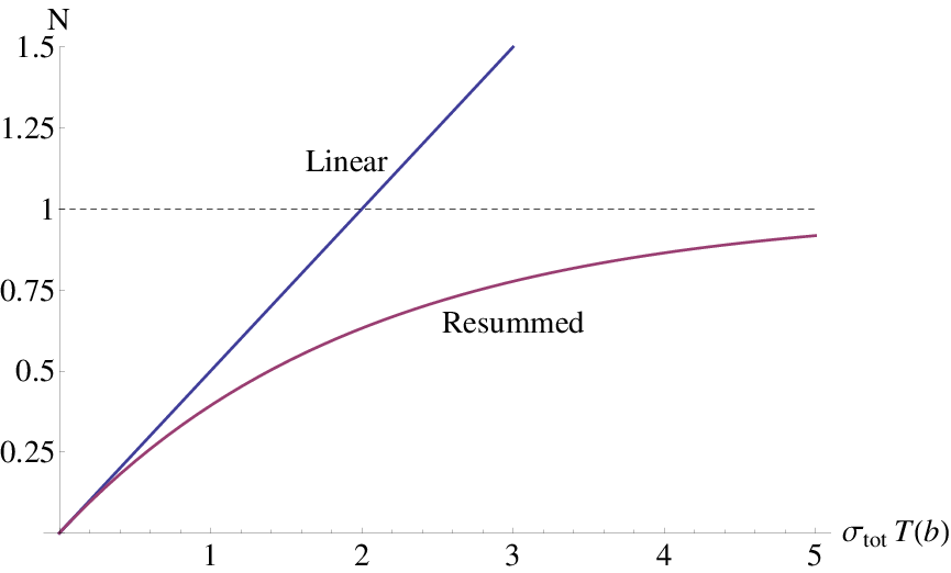
To make this expression more concrete, we can model the nucleons as dipoles, using from (3.40) in (3.52), which, in the small-dipole / large-dipole asymptotic limit (3.39) gives
| (3.54) |
Comparing the Glauber-Gribov-Mueller (GGM) multiple scattering amplitude (3.52) with the single-nucleon scattering amplitude , we see (as in Fig. 3.12) that in the limit of low densities , the resummed amplitude reduces to the linear one. However, at high densities, the linear amplitude can grow without bound, while the exponential form of (3.52) gives an amplitude which saturates to unity (see Fig. 3.12). The growth of the forward amplitude without bound would constitute a violation of unitarity [78], reflecting a scattering probability greater than . Multiple scattering effects are thus important for the unitarization of the dipole-nucleus scattering cross-section.
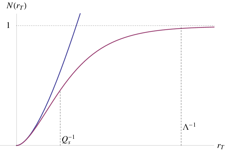
To further unfold the implications of the GGM formula, let us examine the dependence on the dipole size. As we saw in (3.39) and (3.40), the perturbatively small DIS dipole measures the strength of the gluon field of the nucleon, with a coupling proportional to the dipole moment squared of the small dipole. Thus, as increases, the strength of the scattering amplitude increases, reflecting the increased coupling of the dipole to the external field. This is true as long as the dipole is small, interacting with a larger, nearly uniform color field. For the general case of two dipoles interacting, (3.40), the growth of with is softened (although not cut off) when the small dipole becomes comparable in size to the large one (the “nucleon”) at . However, in the resummed amplitudes (3.53) and (3.54), the momentum scale that multiplies is different: it has been enhanced by the density factor . This momentum scale is known as the saturation scale , and it can be either defined implicitly from (3.53) as the point at which the magnitude of the exponent becomes unity,
| (3.55) |
or explicitly from the dipole form (3.54) as 33 3 For from a single quark rather than a dipole, the value of is half this.
| (3.56) |
so that (3.54) becomes
| (3.57) |
As shown in Fig. 3.13, the growth of with turns over at rather than at when the effects of multiple scattering have become important. This suggests that, in the high transverse densities of a Lorentz-contracted nucleus, the transverse sizes over which the color fields are uniform are much smaller, of order . The color fields of many independent nucleons in the large- limit are randomly distributed in color space, so that the superposition of these fields seen by the DIS dipole tends to dilute the color fields of the nucleons. Thus the effect of high transverse densities is to shorten the size of the correlated “color domains” in the transverse plane from to , as visualized in Fig. 3.14. This is another manifestation of nuclear shadowing through multiple rescattering effects. Since , we see that scales parametrically as ; it is a dynamical scale generated by the resummation of coherent multiple rescattering.

Finally, let us note that, despite the apparent quantum loops generated by multiple gluon exchange with the nucleus, in the resummed diagrams of Fig 3.11 these loops have all been cut. Thus our summation of the leading- contributions contains no genuine quantum corrections; it therefore appears that the Glauber-Gribov-Mueller formula (3.53) and the emergence of the saturation scale (3.56) are classical effects. If the leading- effects considered here are truly classical in origin, we should be able to recover them by analyzing the classical equations of motion of QCD; this is the approach we pursue in the next Section.
3.2 The McLerran-Venugopalan Model: Classical Gluon Fields of a Heavy Nucleus
3.2.1 Yang-Mills Equations for High-Energy Point Charges
Motivated by the Glauber-Gribov-Mueller formula (3.52) for deep inelastic scattering on large nuclei, we wish to consider the small- gluon wave function of an ultra-relativistic heavy nucleus in the classical limit. This approach was pioneered in [69, 70, 71] and is known as the McLerran-Venugopalan (MV) model of a heavy nucleus. Such a wave function would be a solution of the classical Yang-Mills equation
| (3.58) | ||||
for a nucleus under Regge kinematics. When the nucleus is boosted to high energy in the center-of-mass frame considered in Sec. 3.1.3, the color current is purely in the light-cone plus direction. For simplicity, let us consider the nucleus to be a superposition of point charges with positions moving along the light-cone plus axis. Then the current is given by
| (3.59) | ||||
where the factor of 2 arises from the choice of metric. The color quantum number of the current is carried by the fundamental generators , reflecting the color field radiated from the charge; thus the matrix acts on the internal color-space of the charge, rotating its fundamental color quantum number from to . This is to be distinguished from “external” color matrices which are often contracted with quantities such as to form color matrices with definite gauge-transformation properties.
Our goal is to solve (3.58) for the source current given by (3.59) and analyze the results to see if the high transverse densities due to the boost generate saturation effects analogous to the Glauber-Gribov-Mueller calculation (3.53). To solve (3.58), let us first consider the limit of parametrically weak coupling , so that nonlinear effects involving the self-interaction of the fields are suppressed. The weak-field limit is also the Abelian limit of the theory, since the nonlinear terms are dropped, simplifying the field-strength tensor to . In this limit, the Yang-Mills equations reduce down to just the linear Maxwell’s equations
| (3.60) |
Fixing the gauge to be the covariant gauge 44 4 This is also known as the Lorenz gauge, and it is equivalent to the Feynman gauge. When we construct the solution, we will see that it satisfies and thus is also equivalent to the “light-cone gauge of the projectile.” eliminates the term coming from the left-hand side, leaving
| (3.61) | ||||
We note that the transverse and minus components can be trivially solved by , and we solve the plus equation as follows. Since the source is -independent, the solution should be as well; this realization means that the action of coming from the D’Alembertian vanishes. This reduces the left-hand side to , with the only -dependence in the source coming from a set of delta functions. Since the dynamics are now entirely transverse, the solution must also reflect this localization in . Thus we define
| (3.62) |
which reduces (3.61) down to the 2-dimensional Poisson equation
| (3.63) |
This 2D Poisson equation is exactly the same as that for the electrostatic potential from an infinite line of electric charge, with the solution given in any elementary textbook: a logarithmic potential. Writing down the general form of the solution for and applying the Laplacian gives
| (3.64) | ||||
Finally, comparing (3.64) with (3.63) gives the general solution to (3.60) in the weak-coupling limit as
| (3.65) | ||||
where we have included a subscript to emphasize that this is the solution in covariant gauge. The picture of the gluon field in this gauge is of a “shockwave” localized in that radiates out in the transverse direction with a logarithmic potential. The fact that we recover an elementary result from classical electrodynamics is not surprising, since the assumptions that led to (3.65) reduced the Yang-Mills equations (3.58) down to Maxwell’s equations (3.60). However, when we relax the weak-field assumption and examine the full nonlinear equations, we find that (3.65) is still the solution of the full Yang-Mills equations, because all of the nonlinear terms in (3.58) in this gauge are proportional to either
| (3.66) |
Therefore (3.65) is the full solution to (3.58) in covariant gauge, retaining the simple physical interpretation carried over from classical electrodynamics.
However, it is difficult to directly interpret the gauge field (3.65) in terms of gluons because, as we saw in (2.95), a gauge-invariant definition of gluon number invokes the field in the light-cone gauge . Therefore, to interpret (3.65) we would like to perform a gauge transformation to find the corresponding field in the light-cone gauge. The gauge transformation takes the form of an color rotation that rotates the color quantum numbers of the fermions as in (2.83). If this is the transformation that takes the covariant gauge into the light-cone gauge, then it applies to the gluon field and the field strength tensor as
| (3.67) | ||||
where it is to be emphasized that the color matrices used in formulating these transformations are “external” and operate in a different color space than the “internal” color matrices that act on the fermions.
We can determine the form of the light-cone gauge fields most straightforwardly by going through the field-strength tensor as an intermediary. In the covariant gauge (3.65), there is only one nonzero component of the field-strength tensor: . Since the gauge transformation (3.67) only multiplies this by a color factor, this remains the only nonzero component in the light-cone gauge. In both gauges, these tensors are uniquely determined by one component of the gauge field, so we can use (3.67) to immediately write
| (3.68) |
By integrating this expression over , we can solve for the light-cone field , which is necessarily the only nonzero component in the light-cone gauge,
| (3.69) | ||||
where we have chosen the boundary condition at infinity to fix the residual gauge freedom. Using the covariant-gauge field (3.65), we find
| (3.70) |
where we have used the fact that the gauge transformation (3.67) acts on the external color matrix, not on the quark color matrices. Apart from the net color rotation provided by , the main difference between the light-cone field in (3.70) and the covariant field is that the light-cone fields have the structure of a theta function instead of a delta function. The color fields emitted by the point charges flow “downstream,” affecting everything at values greater than the value at the source. The light-cone fields also decay as , unlike the covariant-gauge fields that are logarithmic in the distance.
To fully specify the light-cone field (3.70), we need to determine the precise form of the color rotation . This can be done by defining in (3.67), which we can rewrite as
| (3.71) |
If and were scalars instead of matrices, the solution to this equation would simply be an exponential. Since they are matrices, however, the order of the factors matters and the solution is a bit more subtle. To see the form of the solution, consider iterating (3.71) twice:
| (3.72) | ||||
We see that every iteration introduces another copy of the factor in brackets, evaluated at different points. The largest values in are farthest to the right, with successively smaller values of on the left. This expression has the form of a path-ordered exponential, with the integral in the exponent starting from and traveling out toward if we were to continue iterating (3.72). The only other subtlety is that the infinitesimal step length in the usual form of the path-ordered exponential is with the discretization number. In (3.72) the step lengths are moving toward the initial point ; thus we introduce an extra minus sign in the factors in brackets when we put this into the standard form of the path-ordered exponential. The resulting solution is
| (3.73) |
for the color factor which transforms from covariant gauge to light-cone gauge. Inserting the specific form of the covariant-gauge field (3.65) gives
| (3.74) | ||||
where an extra minus sign is generated by picking up the delta function in an integral running in the negative direction. Since each of the color matrices , as well as the external color matrix all operate in different color spaces, they all commute with each other. Thus the summation in the exponent can be converted into an ordinary product of individual exponential factors, and the path-ordering operator arranges these factors with the terms corresponding to on the right:
| (3.75) | ||||
where the notation of the product in the last line emphasizes the ordering of the factors in from left to right with increasing . The specific color rotation (3.75), together with the spacetime structure given in (3.70) fully specifies the gluon field in the light-cone gauge which is the solution of the classical Yang-Mills equations (3.58) for the source (3.59).
3.2.2 The Non-Abelian Weizsäcker-Williams Field
The Weizsäcker-Williams “equivalent photon approximation” [113, 91] in QED describes the classical radiation of effectively on-shell photons from a high-energy source. Its generalization to QCD is the non-Abelian Weizsäcker-Williams field [61] of gluon radiation, defined as
| (3.76) | ||||
The Weizsäcker-Williams field counts the number of gluons produced per unit , per unit rapidity in the classical state of a nucleus . The factor of arises from the integration over the azimuthal direction ; the lack of dependence of (3.76) on the direction implicitly assumes an unpolarized state. The averaging in the second line is over the three-dimensional positions of charges in the nucleus.
The definition (3.76) in terms of a gluon number density with fixed transverse momentum recalls the definition of transverse-momentum-dependent parton distribution functions (TMD’s) from Chapter 2. Indeed, if we compare (2.99) with (3.76), we see that same operator appearing in the Weizsäcker-Williams field occurs as a specific projection of the gluon field correlator (2.95):
| (3.77) | ||||
where , defined in (2.101), is the unpolarized gluon TMD and the factor of plays the role of the density in the plane wave state as in (2.81). Note that (3.77) only holds at the lowest (classical) order in which the gauge link (2.84) can be neglected. Relating the Weizsäcker-Williams field to the gluon TMD gives 55 5 In making the transition from a quantum-mechanical plane-wave state to a classical state which is localized in position and momentum, care must be taken to account for the normalization of the states. This can be done rigorously by using quantum-mechanical states constructed along the lines of the Wigner distributions of Chapter 5 and fixing the normalization so that the spatial integral recovers the momentum-space expectation value as in (3.77). One then sees that the volume factor is replaced by an average over the spatial density as in (3.76).
| (3.78) | ||||
where we have used the relation (2.95) between the gluon creation / annihilation operators and the light-cone gauge fields. For the nucleus composed of point charges in (3.59), the classical fields are given by (3.70).
The fields are proportional to for the contribution of the charge, and similarly for . All of the charges are contained within the highly Lorentz-contracted nucleus and therefore have positions that are all very close together, of order . For the small- part of the Weizsäcker-Williams field which is relevant for the Regge limit, , so the typical separation between and in the Fourier transform is much larger than the separation between the individual charges . Therefore, for the purposes of the Fourier transform, we approximate the light-cone fields as
| (3.79) |
which effectively takes all of the charges at the same point (). Then the and integrals just generate a combined factor of , so that the Weizsäcker-Williams field of the nucleus is
| (3.80) | ||||
In this classical calculation, the expectation value corresponds to averaging over the positions and colors of the point charges in the nucleus. The color averaging simplifies the expression because each point charge has its color averaged separately, corresponding to a factor of and a trace over the color matrices acting in the color space of . Since , the color averaging gives zero unless ; then . This simplification gives
| (3.81) | ||||
where now only the spatial averaging over and the sum over remain. Note from (3.75) that the color rotation depends on the positions of all the point charges with longitudinal coordinates earlier than the endpoint at : . To explicitly separate out this dependence, it is convenient to assign the labeling of the point charges in ascending order of , so that , with the number of point charges composing the nucleus. Then the color factor in the trace depends only on the coordinates of the charges , while the vector product affects only the endpoint at . Rewriting (3.81) using this notation gives
| (3.82) | ||||
The spatial averaging over the charge only affects the vector product, so we can carry it out independently. If the nucleus has an average transverse number density of these charges at impact parameter , then the averaging over is given by
| (3.83) | ||||
where we have used the fact that the nuclear density varies only over macroscopic distances proportional to to replace , which is valid whenever . Thus we have
| (3.84) | ||||
where the last step that remains is to compute the net effect of the color rotation due to all of the charges preceding the endpoint .
To evaluate the color factor from (3.84), it is helpful to make use of the following identity that relates Wilson lines in the fundamental and adjoint representations [78],
| (3.85) | ||||
where
| (3.86) | ||||
is the adjoint-representation analog of from (3.75) and is a color matrix in the adjoint representation of . Using (3.85) allows us to simplify the color factor in (3.84) by expressing it in the adjoint representation,
| (3.87) | ||||
where we have used the fact that an adjoint Wilson line is purely real, and stands for a trace over adjoint indices. Inserting this back into (3.84) gives
| (3.88) | ||||
The product form (3.86) of the Wilson line is ordered with the factor corresponding to occurring on the right, since it has the largest value of ; similarly , which is ordered the opposite way, has the factor corresponding to occurring on the left. Therefore we can isolate the dependence on the charge by pulling out the latest factor:
| (3.89) |
In principle the two exponentials contain emissions of an arbitrary number of gluons from each point charge. However, from our analysis in Sec. 3.1.3, we only expect the classical Yang-Mills description to agree with the quantum calculation in QCD up to the level of 2 gluons per color charge as illustrated in Fig. 3.11. Beyond 2 gluons per “nucleon,” we do not expect the classical calculation to agree with the quantum one, because the quantum calculation will include genuine loop diagrams that cannot be reproduced by the classical formula (3.89). Therefore, in seeking to compare with the quantum calculation of Sec. 3.1.3, we should truncate the interaction with point charge at , corresponding to a contribution of 2 gluons per charge to the Wilson line trace. Performing this expansion yields
| (3.90) |
Now that we have factored out the point charge from the others, we can perform the average over its color and spatial coordinate. The color average eliminates the term, since , and in the term gives
| (3.91) |
where is the quadratic Casimir in the adjoint representation. Then the spatial averaging over can be carried out along the lines of (3.83):
| (3.92) | ||||
These logarithmic integrals should be familiar; they arose when we calculated the dipole-dipole scattering cross-section and are most easily carried out in momentum space using (3.26). For brevity we relabel :
| (3.93) | ||||
Comparing with (3.32), we see that this averaged quantity is proportional to , which corresponds to the eikonal scattering of a color dipole on the field of a point charge (3.21). But here there is no dynamical scattering occurring; the effective “scattering” occurs between the point charge which is generating the field and the adjoint Wilson lines occurring in (3.88). The Wilson lines are effectively forming a “dipole” of size which is “scattering” in the field of the point charges making up the nucleus. (See also Fig. 3.15.)
We can evaluate the integral (3.93) straightforwardly by doing the angular integral and employing the small-argument asymptotics of the Bessel function :
| (3.94) | ||||
Substituting (3.94) and (3.91) back into (3.90) gives a full evaluation of the point charge as
| (3.95) |
This procedure systematically evaluates the averaging over the colors and positions of the last color-charge, generating the multiplicative factor in parentheses. Iterating this for all of the charges generates a total of such factors, and the adjoint trace of unity yields a factor of :
| (3.96) |
where we switch interchangeably between the factor in parentheses in the first line and the full exponential in the second line. This is consistent because we have already truncated the exponentials in (3.90) at and also because the quantity is parametrically small, of order .
Substituting (3.95) back into (3.88) gives
| (3.97) | ||||
We identify the color factor in parentheses as , and we can perform the summation directly as a finite geometric series
| (3.98) | ||||
where we have exploited the ability to interchange between the exponential and its expansion. The denominator of (3.98) cancels the other factors in the integrand of (3.97), giving the fully- evaluated Weizsäcker-Williams field as
| (3.99) | ||||
where we have changed variables to the impact parameter and dipole separation .
3.2.3 The Color-Glass Condensate
The form of the Weizsäcker-Williams field (3.99) obtained by solving the classical Yang-Mills equations (3.58) mirrors the form of the dipole-dipole forward scattering amplitude in the Glauber-Gribov-Mueller multiple scattering approximation (3.54) that enters eikonal DIS scattering cross-section. Defining the gluon saturation scale from the exponent in (3.99) to mirror the quark saturation scale (3.56),
| (3.100) |
we see that differs from in two regards: a factor of 2 and a factor of . The factor of 2 arises because (3.56) describes the interaction with target nucleus composed of dipole “nucleons,” whereas (3.100) describes the scattering on a target nucleus composed of point charges. The factor of arises because (3.56) describes the interaction of a projectile composed of a quark dipole in the fundamental representation, whereas (3.99) describes the interaction with a pair of gluon Wilson lines in the adjoint representation. In the adjoint representation, so that .

This parallel between a scattering cross-section and the classical gluon distribution occurs because the light-cone gauge fields necessary to define the number of gluons have the structure of theta functions (3.70). In the light-cone gauge, gluons emitted at later “times” are affected by the pre-existing gluon fields of the earlier sources. This is the origin of the adjoint Wilson lines in (3.88): a gluon emitted at “scatters” in the field generated by the earlier charges, as illustrated in Fig. 3.15. We can carry this interpretation further by noting that the Weizsäcker-Williams field is defined in (3.78) as the expectation value of light-cone gluon fields in a hadronic state . Taking this definition as the classical limit of a quantum operator equation, we can always insert a complete set of final states to obtain the square of a transition amplitude. The same is true of the Weizsäcker-Williams field (3.88) expressed in terms of adjoint Wilson lines; after the insertion of a complete set of states, this describes the scattering cross-section of a gluon dipole on the nuclear target. In analogy with (3.57), we define the (imaginary part of the) forward scattering amplitude of a gluon dipole as
| (3.101) |
in terms of which we can write the Weizsäcker-Williams field as
| (3.102) |
This classical result is independent of the details of the nuclear target and can be obtained even from a continuous charge-density description [114] of the nucleus. This is the central result of the McLerran-Venugopalan model of a heavy nucleus in the classical limit.
We can also gain insight from the calculation of the Weizsäcker-Williams field by interpreting the expectation value as a correlation function of the gluon fields. Comparing (3.78) and (3.99), we identify the correlator as
| (3.103) | ||||
From this expression, we see that is the correlation length of the color fields in the transverse plane. This strengthens the interpretation given in Fig. 3.14 of as the typical transverse size of correlated color domains; here we can see this explicitly at the level of a color-color correlation length.
Furthermore, we observe that the magnitude of the Weizsäcker-Williams field (3.102) is parametrically large, of order , corresponding to individual gluon fields on the order of . In comparison, the fields in the Abelian limit given by the covariant-gauge solution (3.65) are parametrically small: . The uniquely non-Abelian physics, reflected in the nonlinear color rotation matrix present in the light-cone gauge (3.70), has driven the intensity of the fields up by a factor of . This is generically expected for any classical solution of the nonlinear Yang-Mills equations, which we can see trivially by equating the linear and nonlinear terms in the equation of motion (3.58). But it is quite nontrivial that the same physics generates nuclear shadowing and saturation in the Glauber-Gribov-Mueller formula (3.57), which was obtained by the resummation of in a quantum-mechanical calculation. The parametrically strong fields correspond to high gluon occupation numbers consistent with the classical fields. This observation confirms the interpretation of Fig. 3.11 that eikonal scattering on a system of dense color charges corresponds to the interaction with classical gluon fields.
Finally, it is instructive to examine the limits of the Weizsäcker-Williams distribution (3.102) at large and small transverse momentum. Rewriting this using (3.101) gives
| (3.104) | ||||
where in the second line we have neglected the impact parameter dependence for simplicity and generated a trivial factor of the transverse area . In the limit the exponent becomes small; we therefore expand the exponential to the lowest nontrivial order:
| (3.105) |
where the angular-averaged dipole field was defined in (3.35). Thus the large- limit corresponds to short distances inside a single color domain, where the field strength is just a superposition of the perturbative (linear) fields. On the other hand, if we consider the small- limit, , the full exponential becomes small; after dropping it, the Fourier transform generates the familiar logarithm (3.21)
| (3.106) |
Deep in the saturation regime, the infrared divergence that scaled perturbatively as has softened to just a logarithmic one. This means that the phase-space distribution of gluons is infrared finite, going to zero as . And finally, we can estimate the behavior in the saturation regime by neglecting the logarithm in the exponent and performing the integral over analytically. The logarithm is necessary to obtain the right large- asymptotics, but for in the vicinity of this approximation should give the right answer:
| (3.107) | ||||
where is the incomplete gamma function. These results are plotted in Fig. 3.16, illustrating the behavior, the large- asymptotics, and a smooth interpolation between them.
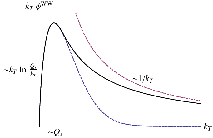
From Fig. 3.16, we see that the phase-space distribution of gluons peaks around . (In (3.107), the peak occurs at ). In a (very) loose analogy with phenomena in condensed-matter physics, this parametrically large concentration of gluons in a single momentum state is sometimes referred to as the color-glass condensate (CGC) (see, e.g. [114, 64, 65, 66, 115, 116, 117, 68, 118]). The nonlinear effects of multiple gluon scattering have shifted the low- gluons up in momentum and depleted the distribution in the far infrared. The saturation scale is a measure of the density of the system, scaling with the number of charges as , so by increasing the density of charges, we further deplete the infrared region. This leads to a profound conclusion: since emerges as a dynamical infrared cutoff that increases with the density of the system, for a system of sufficient density that , the physics of high-energy scattering can be made perturbative! Indeed, calculations of the scale at which the coupling runs in typical high-energy collisions confirm that they are proportional to (see, e.g. [119]). Thus, the emergent physics of saturation provides a well-defined resummation of QCD itself in which high-energy scattering becomes perturbative and classical fields dominate:
| (3.108) |
Thus the CGC approach, characterized by the Glauber-Gribov-Mueller and McLerran-Venugopalan formalisms, is a powerful tool which can bring high-energy, high-density hadronic processes into the perturbative domain.
3.3 Comments on Small- Quantum Evolution
In this Chapter we have discussed the role of strong classical gluon fields arising from a system such as a heavy nucleus with a natural parameter , the nucleon number, parameterizing the large transverse density. This external parameter makes it possible to re-sum the interactions with the large density of partons in a systematic manner. However, this is not the only manner in which a system with a high density of partons can arise. A much more physically achievable - if more calculationally difficult - route to the dense limit is through the effects of quantum evolution. A full discussion of the role of quantum corrections is beyond the scope of this document. However, to put the results of the previous Sections in context, it is necessary to at least describe the role of quantum evolution in generating systems of high-density to which the CGC formalism can be applied. Thus, in this Section, we will summarize and motivate the physics of high-energy, small- quantum evolution without explicit derivations. For discussions of quantum evolution, the reader is referred to the works of [78, 20].
“Quantum evolution” refers to the re-ordering of the perturbation series that occurs when certain classes of quantum corrections which are usually suppressed by the coupling become parametrically enhanced. In deep inelastic scattering in the Bjorken regime, for example, the collinear splitting of partons is suppressed by a power of the coupling but systematically enhanced by a large logarithm of the photon virtuality . If the virtuality becomes large enough that becomes , then the logarithm can fully offset the suppression by , making these quantum corrections equal in importance to the tree-level processes. When this is true, all such diagrams which are maximally enhanced by any power of must be re-summed. This can be done by formulating a differential evolution equation describing how observables are affected by one such enhanced quantum correction; for the collinear splitting enhanced by large logarithms of , this evolution equation is the Dokshitzer-Gribov-Lipatov-Altarelli-Parisi (DLGAP) equation [51, 52, 53]. The solution to the DGLAP equation then re-sums all orders of .

A similar situation occurs in high-energy scattering in the Regge limit. When eikonal scattering processes such as the quark-quark scattering of Fig. 3.2 take place, they are kinematically insensitive to the emission of additional small- gluons through bremsstrahlung (Fig. 3.17, left panel). This radiation of an extra gluon during the eikonal scattering is suppressed by a power of compared to the process of Fig. 3.2, but it is enhanced by the phase space available for soft gluons: . Thus, for the inclusive observables to which these diagrams contribute, the overall power-counting of the quantum correction is . As the energy of the scattering process is increased, the amount of phase space available for the emission of low- gluons increases; thus, when the energy is sufficiently large that , all such quantum corrections must be re-summed. This leads to the quantum evolution equation known as the Balitsky-Fadin-Kuraev-Lipatov (BFKL) equation [54, 55], which describes the development of a small- gluon cascade (Fig. 3.17, center panel).
The bremsstrahlung corrections embodied in the BFKL equation lead to a gluon distribution that grows at small- as [78]
| (3.109) |
where the numerical value was obtained for . Since the number of gluons generated through bremsstrahlung increases with energy, the total scattering cross-section (3.33) also grows. Both the apparent increase in the density of gluons and the rapid growth of the scattering cross-section with energy (and hence, with decreasing ) are in tension with the constraints imposed by the unitarity of the -matrix. The Froissart-Martin bound, for example, derives from unitarity the constraint that the cross-section can grow at most as [56, 57, 58], while (3.109) gives rise to a cross-section that grows as . These considerations indicate that the growth of gluon density due to bremsstrahlung cannot continue unabated forever, down to arbitrarily small- (or arbitrarily high energies).
Eventually, the densities of gluons become sufficiently large that nonlinear effects, like those discussed in this Chapter, become important. When the density of gluons becomes sufficiently large, newly-radiated gluons are likely to scatter on the dense fields that already exist. The analogous role to the GGM multiple scattering discussed in Sec. 3.1.3 is played by gluon fusion, which limits the total rate at which the gluon density can grow (Fig. 3.17, right panel). Since the rate of gluon bremsstrahlung is proportional to the total number of gluons in the cascade, but gluon fusion is proportional to its square , this can be used to estimate the momentum scale at which the nonlinear effects become important. The result is [59, 60, 78]
| (3.110) |
where is the transverse area. This estimate agrees completely with the calculation from the GGM multiple-scattering formalism (3.55) after the conversion between the scattering of fundamental-representation quarks and adjoint-representation gluons.
Thus the physics of saturation can also be obtained by the small- quantum evolution of collisions at very high energies. When nonlinear effects are systematically included in the small- evolution equations, the BFKL equation is replaced by the Balitsky-Kovchegov (BK) equation [62, 63], which explicitly satisfies the unitarity bound. Equivalently, in the continuous charge-density formulation of the MV model, the evolution equation is known as the Jalilian-Marian–Iancu–McLerran–Weigert–Leonidov–Kovner (JIMWLK) functional differential equation [64, 65, 66, 67, 68]. The (approximate) solutions to these equations give a saturation scale that grows with energy (or decreasing ) as
| (3.111) |
where the final numerical value was obtained using . As the energy of the process is increased (and decreased), gluon bremsstrahlung generates more color charges, increasing and decreasing the radius of the correlated color domains. Therefore, small- evolution equations suggest that the perturbative limit described by the CGC formalism is also reached in the limit of high energies through quantum corrections. The essential physics of saturation at high charge densities applies both to a proton at high energies through quantum evolution equations, and to a heavy nucleus in the initial conditions of those equations [120, 121, 122, 123].
Therefore we can consider the scattering on a heavy nucleus discussed in this Chapter as a metaphor for the more general situation of scattering on a high-density system. The physical conclusions reached by using the GGM or MV formulas can be carried over and applied to a proton at very high energies, even though the quantitative details of their application may change [78]. For this reason, we will use the saturation formalism in terms of a heavy nucleus presented here as a window into the application of the spin- and transverse-momentum physics discussed in Chapter 2 to systems of high density. In Chapter 4 we will discuss saturation effects in the generation of single transverse spin asymmetries by the scattering of a polarized projectile on an unpolarized target. In Chapter 5 we will study the reverse situation, examining saturation effects in a polarized target by generalizing the MV model of Sec. 3.2 to include spin and transverse momentum.
Chapter 4 Transverse Spin as a Novel Probe of Saturation
Consider the single transverse spin asymmetry (STSA) (2.61) produced in high-energy proton collisions . The rapidity of the tagged hadron is defined as
| (4.1) |
where we have used the on-shell condition . If we choose a frame in which the polarized proton moves along the axis with large momentum and the unpolarized proton moves along the axis with large momentum , then the total rapidity interval between the colliding protons is
| (4.2) |
where is the center-of-mass energy (squared) of the collision.
Experimental measurements of the STSA at Fermilab and at RHIC indicate that the asymmetry produced in these collisions is small for most of the kinematic range, but becomes quite large when the rapidity of the tagged hadron is close to the rapidity of the polarized proton [34, 1, 33, 35, 36, 37, 38, 39, 40, 41, 2, 42]; that is, when the rapidity interval is small. We can translate from the rapidity to the longitudinal momentum fractions of the tagged hadron with respect to the polarized and unpolarized protons, respectively, as
| (4.3) | ||||||
by straightforward application of (4.1). When , we can expand (4.3) to find
| (4.4) | |||||
Under these highly-asymmetric kinematics, the scattering process is most sensitive to the large- valence region in the polarized proton, and the small- bremsstrahlung region in the unpolarized proton. As we have seen in Chapter 3, the small- regime is characterized by a high density of gluons that gives rise to the saturation paradigm of high-energy scattering.
These considerations suggest that the asymmetry generated in these high-energy proton collisions reflects the spin-dependent interaction of the polarized projectile with the dense, classical gluon fields of the unpolarized target. Since, as discussed in Sec. 2.1.3, the STSA is a -odd observable, this suggests that the polarized proton is acting as a unique probe of the -odd component of the classical gluon fields. The dominant gluon fields which drive the unpolarized observables described in Chapter 3 are manifestly -even, so the high-density physics which gives rise to STSA must be fundamentally different from the conventional channels of high-energy scattering. In this Chapter, we will analyze the generation of STSA from these -odd gluon fields, which are known in the literature as the “odderon.”
Since the asymmetry is generated from the valence region of the polarized proton, a useful proxy for the full proton wave function is a single transversely-polarized valence quark which proceeds to scatter on the classical gluon fields of a dense unpolarized target. As we saw in Sec. 3.2, a useful realization of this dense target is a heavy nucleus in the McLerran-Venugopalan model. Thus we can consider the scattering of a transversely-polarized quark on a heavy nucleus as a simple implementation of saturation effects in the far forward regime of collisions. The goal is then to find the leading-order channels through which the transverse spin dependence enters in the saturation framework.

In this Chapter, we will consider the STSA of quarks, gluons, and prompt photons produced in polarized collisions: . This process is illustrated in Fig. 4.1, where the high energy interaction between the projectile quark and the target nucleus is schematically denoted by gluon exchanges. To introduce the methodology, we will first concentrate on the quark production process, . Certainly keeping only the eikonal interaction of the polarized quark with the target would not generate the STSA, since the eikonal scattering (3.21) is independent of the quark polarization. A non-eikonal correction has to be included somewhere: in the multiple-rescattering Glauber-Gribov-Mueller [77] approximation discussed in Sec. 3.1.3, the non-eikonal rescattering corrections are suppressed by powers of energy and are very small. A much larger spin-dependent contribution comes from the non-eikonal splitting of the projectile quark into a quark and a gluon, , which is suppressed only by a power of the strong coupling . In the language of light-cone perturbation theory (LCPT), the splitting may take place either before or after the interaction with the target, as shown in Fig. 4.2. Splitting during the interaction with the target is suppressed by powers of energy due to the instantaneous nature of eikonal scattering [124].

The lowest-order diagrams shown in Fig. 4.2 that contribute to STSA in contain the emission of a single gluon from the polarized quark, where both the gluon and quark can scatter in the field of the target. Multi-gluon non-eikonal emissions and quark pair-production are also possible, but they are higher-order in and, hence, outside of the leading-order precision of this work. The spin dependence of the process illustrated in Fig. 4.2 originates within the light-cone wave function of the quark-gluon system, which couples to the interaction in a way that generates the asymmetry. In Sec. 4.1, we will first outline the calculation of the light-cone wave function using LCPT. Then we will combine the resulting splitting wave function squared with the quark and gluon interactions in the field of the target and identify the contribution to the asymmetry. In the end we obtain general expressions for quark, gluon, and photon STSA’s in our formalism. The incoming light quark has a particular flavor ; multiple quark flavors can be incorporated into our formalism by convoluting the obtained cross sections with quark distributions corresponding to different flavors (inserting the appropriate quark masses into our results below). As discussed above, we choose a frame in which the incoming projectile quark is moving along the light-cone -axis, while the target is moving along the -axis, and we will work in the light-cone gauge of the projectile, (which is equivalent to the covariant gauge , as discussed in Sec. 3.2.1). The analysis in this Chapter is original work which follows closely our paper [125].
4.1 General Result: Coupling Spin to Interaction C-Parity
Recall that the single transverse spin asymmetry, first defined in (2.61), is given by
| (4.5) |
We will determine which parts of the wave function and the interaction couple to the numerator and the denominator of the asymmetry.
4.1.1 Light-Cone Wave Function and Transverse Polarization
Consider the splitting shown in Fig. 4.3 of a transversely polarized quark with momentum and polarization decaying into a gluon (with momentum , polarization , and color ) and a recoiling quark (with momentum and polarization ). The projectile quark is traveling along the light-cone -direction and the recoiling quark carries a fraction
| (4.6) |
of the incoming quark’s longitudinal momentum. We do not restrict ourselves to the case of an eikonal quark emitting a soft gluon (), but work in the general case when both the quark and the gluon can carry comparable longitudinal momenta. We do, however, assume for simplicity that to be able to neglect the contribution of virtual corrections proportional to . These corrections are discussed in the paper [125].

The calculation of the light-cone wave function corresponding to the diagram in Fig. 4.3 is different from other similar calculations in the literature (see e.g. [126, 127]) only in that now the incoming quark is polarized transversely. For this, we use the transverse spinors with polarization along the -axis first defined in (2.52). It is convenient to also use the same spinor basis (2.52) for the outgoing quark in Fig. 4.3 as well. Using the standard rules of LCPT [95, 128] with this spinor basis, we evaluate the light-cone wave function shown in Fig. 4.3 as
| (4.7) |
where
| (4.8) |
is the gluon polarization vector with the transverse components .
In arriving at (4.7) we have used the fact that the incoming state in Fig. 4.3 contains only the quark with momentum while the intermediate state contains the quark and the gluon, as denoted by the vertical dotted line in Fig. 4.3. For diagrams with initial-state interactions where the polarized quark scatters in the nucleus before the gluon emission, as shown in the right panel of Fig. 4.2, the roles are reversed: the quark line is the intermediate state, and the quark–gluon system is the final state. Since , the energy denominator reverses sign for final-state splittings. The wave function (4.7) is also normalized differently from [78] and will require a compensating factor when we calculate the cross-section using the rules of LCPT.
Using the on-shell conditions explicitly gives the terms entering the energy denominator:
| (4.9) |
The relevant spinor products can be straightforwardly tabulated from (2.52) and (2.1.2) as 11 1 Note again that becomes a spinor for a transversely polarized particle only for : Eqs. (4.10) give us the matrix elements for spinors related to the Brodsky–Lepage spinors via (2.52), which do not necessarily correspond to transverse polarizations in the general case.
| (4.10) | |||||
| (4.11) | |||||
and the matrix element does not contribute to since in the light-cone gauge. Here , . With the matrix elements (4.10) it is straightforward to evaluate the light-cone wave function (4.7) in momentum space, obtaining
| (4.12) | ||||
where
is a natural effective mass parameter in the wave function and are the SU() generators in the fundamental representation.
Now we can Fourier transform the wave function to coordinate space
| (4.13) |
with the transverse coordinates defined in Fig. 4.3. Since the momentum-space wave function depends only on , one of the two integrals can be performed to yield a delta function . Performing the remaining momentum integral in (4.13) yields modified Bessel functions
| (4.14) | ||||
It is useful to separate out the color factor and the delta function from the rest of the wave function (denoted by ), such that
| (4.15) |
Finally, we need to square the wave function and sum over the final particles’ polarizations. Here we are interested in producing a quark with a fixed transverse momentum, while integrating over all transverse momenta of the produced gluon in Fig. 4.2. As we will show when we calculate the cross-section in Sec. 4.1.2, this will set the gluon’s transverse coordinate to be the same both in the amplitude and in the complex conjugate amplitude, while the quarks will have different transverse coordinates between the amplitude and the conjugate amplitude (since their momentum is tagged). See Fig. 4.6 below for the illustration of the full amplitude squared. The “square” of the light cone wave function (4.14) with the above rule for the quark and gluon transverse coordinates is illustrated in Fig. 4.4.

The wave function (4.14) squared as shown in Fig. 4.4 contains one contribution which is polarization-independent and another which is proportional to the quark polarization eigenvalue
| (4.16) | ||||
Substituting the wave function (4.14) into (4.16) and performing the sums gives the unpolarized part as
| (4.17) | |||||
and the transversely-polarized part as
| (4.18) | ||||
Note that is a scalar under rotations in the transverse plane and is parity-even, whereas has an explicitly preferred azimuthal direction (i.e., the axis) and is parity-odd since it “knows” about the transverse polarization of the incoming quark. The axis can be written as the direction of the vector, since the incoming quark with momentum is moving along the axis, while being polarized along the axis, such that . We show in Sec. 4.1.3 that the unpolarized part of the wave function squared contributes to the unpolarized quark production cross section , while the polarization-dependent part of the wave function squared generates the spin-asymmetric cross section .
4.1.2 Target Interactions in Quark Production
Having computed the light-cone wave function, we can now construct the scattering cross section by allowing the wave function to interact with the small- field of the target nucleus. It is well known [62, 115] that eikonal quark and gluon propagators in the background color field can be correspondingly written as fundamental and adjoint path-ordered Wilson lines as in (3.23)
| (4.19) | |||||
| (4.20) |
where ’s are the SU() generators in the adjoint representation and the projectile is moving along the light-cone -axis. In essence, this means that the the projectile’s transverse position is not altered during the scattering, and the effect of the target field is to perform a net SU() color rotation on the projectile. The Wilson lines resum these interactions and give the total phase of that color rotation. They are illustrated in Fig. 4.5. Note that the adjoint Wilson line is real-valued.

The Wilson-line approach is quite generic: if the target gluon field is quasi-classical, as in the case of the McLerran–Venugopalan (MV) model [70, 71, 69] discussed in Sec. 3.2, then correlators of the Wilson lines resum powers of corresponding to the Glauber-Gribov-Mueller (GGM) multiple-rescattering approximation [77] of Sec. 3.1.3. Non-linear small- evolution resumming powers of can be included into the correlators of the Wilson lines through the Balitsky–Kovchegov (BK) [62, 129, 130, 63, 131] and Jalilian-Marian–Iancu–McLerran–Weigert–Leonidov–Kovner (JIMWLK) [114, 64, 65, 66, 115, 116, 117, 68, 118] evolution equations mentioned in Sec. 3.3. Thus expressing the interaction with the target in terms of the Wilson lines (4.19) allows for several different levels of approximation for this interaction.

The scattering amplitude for quark production is composed of two sub-processes: the splitting of (4.14) calculated in Sec. 4.1.1 and the Wilson line scattering (4.19) of the quark and the gluon in the field of the target. These elements give two distinct diagrams contributing to the scattering amplitude shown in Fig. 4.2 above for . To find the quark production cross section we need to square the diagrams in Fig. 4.2, keeping the transverse momentum of the quark fixed, as depicted in Fig. 4.6. As discussed above, this implies that the transverse coordinates of the quark are different on both sides of the cut. Just like in other similar calculations [124, 127], the splitting may occur with either initial-state or final-state interactions with the target, both in the amplitude and in the complex conjugate amplitude, resulting in the four different terms shown in Fig. 4.6. Diagrams with both initial- and final-state interactions correspond to splitting during the brief interaction with the target, which is suppressed by the center-of-mass energy [124].
Using Fig. 4.6 we can write down the expression for the energy-rescaled, color-averaged amplitude squared in terms of Wilson lines and the wave function responsible for the splitting, remembering to reverse the sign in the wave function for splitting occurring after the interaction:
| (4.21) | |||||
where is the number of colors, the traces are taken over the fundamental representation indices, and summation is implied over repeated adjoint color indices. Substituting Eq. (4.15) into (4.21) and using the identities (c.f. (3.85))
| (4.22) |
for arbitrary matrices , we find
| (4.23) |
where the factor responsible for the quark’s interaction with the target, denoted by , is given by
| (4.24) | ||||
Here is the fundamental Casimir operator of SU(), and the angle brackets on the right denote averaging over the field configurations of the target.
Defining the -matrix operator for a fundamental-representation color dipole by
| (4.25) |
we can rewrite more compactly as
| (4.26) | ||||
As we have already mentioned, this interaction with the target can be evaluated either in the Glauber-Gribov-Mueller multiple-rescattering approximation of Sec. 3.1.3 or using the JIMWLK evolution equation.
The expression (4.26) simplifies in ’t Hooft’s large- limit [79], which corresponds to taking the number of colors to be large and the coupling to be small such that the product is constant:
| (4.27) |
In this limit, the correlators of several single-trace operators factorize, such that, for instance, [62, 63, 132]. Defining
| (4.28) |
we rewrite (4.26) in the large- limit as
| (4.29) |
To compute the quark production cross sections, we need to Fourier transform the coordinate space amplitude squared of (4.23) back to momentum space and include the appropriate kinematic factors. We will now derive the relation between and the cross-section; for this it is useful to label the momenta of the incoming and outgoing particles as in Fig. 4.7 without imposing momentum conservation a priori, since it will be handled explicitly by the formulas.

The standard expression for the cross-section is [91]
| (4.30) | ||||
where , , and is the usual scattering amplitude as calculated from Feynman diagrams. Light-cone perturbation theory (LCPT) relates the cross-section to an amplitude which has been rescaled by the center-of-mass energy as in (3.21); also, to use the LCPT rules given in [78], we need to account for a different normalization of the wave function (4.14). Thus we define
| (4.31) |
Additionally, we can use the dominant kinematics to simplify the delta function:
| (4.32) |
using (4.31) and (4.32) in (4.30) gives
| (4.33) |
where we have used the delta function (4.32) to integrate over and . Now, Fourier-transforming the amplitude and complex-conjugate amplitude
| (4.34) | ||||
we see that the integral in (4.33) will generate a delta function which sets the coordinate of the untagged gluon equal in the amplitude and complex-conjugate amplitude. Altogether, this gives the expression for the cross-section in terms of (4.23) as
| (4.35) |
with and the transverse momentum and rapidity of the produced quark. Integrating over the delta functions from the wave function in (4.23) imposes the kinematic constraints
| (4.36) | |||
| (4.37) |
which relate the quark coordinates before and after the splitting and describe the non-eikonal quark recoil. To make the incoming quark transversely polarized we need to put the transverse momentum of the incoming quark to zero: . We thus obtain the general result for quark production in scattering
| (4.38) |
with from (4.16) and from (4.26). The expression (4.38) contains multiple rescatterings and non-linear small- evolution between the projectile and the target. Note that it does not resum the small- evolution between the produced quark and the projectile (which can be included following [127]), and hence is not valid for very small (i.e., the values of are restricted by ). Since, as we will see below, both the experimental STSA and the STSA resulting from our production mechanism fall off with decreasing , the region of interest in this work corresponds to not being very small, where (4.38) is fully applicable.
4.1.3 Spin, Asymmetry, and C-Parity in Quark Production
Using (4.38) we can explicitly determine the parts of the wave function (4.16) and the interaction (4.26) which couple to the numerator and denominator of the asymmetry (4.5). In Sec. 2.1.3 we demonstrated that the reversal of transverse spin is equivalent to a transverse rotation which reverses the direction of the transverse momentum (see Fig. 2.4). This was the reason for the two equivalent definitions of STSA as written in (4.5).
Therefore we can project out the symmetric part of the cross-section by explicitly symmetrizing (4.38) with respect to both spin flip and momentum reversal . Similarly, we can project out the antisymmetric part by explicitly antisymmetrizing (4.38) under spin flip and momentum reversal. Since the eikonal interaction (4.26) is independent of the spin eigenvalue , the (anti)symmetrization with respect to spin simply selects the polarized (4.18) or unpolarized (4.17) parts of the wave function squared; thus we write
| (4.39) | ||||
where the relative factor of between and arises because is defined as the full difference between the cross-sections rather than the half-difference.
Reversing the transverse momentum is equivalent to interchanging the coordinates in the Fourier factor, and we note that both the polarized (4.18) and unpolarized wave functions (4.17) are invariant under this exchange. Thus the (anti)symmetrization under spin flip only affects the wave functions, while the (anti)symmetrization under momentum reversal only affects the interactions:
| (4.40) | ||||
These (anti)symmetric combinations of spin-dependence in the wave function and dependence in the interaction are the only ones which are consistent with rotational invariance as illustrated in Fig. 2.4. An explicit cross-check verifies that the other combinations are identically zero for precisely this reason [125].
Motivated by this observation, we define the symmetric and antisymmetric parts of the interaction as
| (4.41) |
To understand the meaning of this symmetrization, let us note that in the dipole trace (4.28), the Wilson line of a quark in the complex-conjugate amplitude is equivalent to the Wilson line of an antiquark in the amplitude [133, 134]. Thus the interaction (4.26) for this quark production process can be expressed in terms of quark-antiquark color dipoles (4.28). The exchange of coordinates then is equivalent to swapping the roles of the quark and antiquark. This is accomplished by charge conjugation , which indeed transforms the Wilson lines and dipole operators as
| (4.42) | ||||
Thus it is natural to decompose each dipole -matrix into the even and odd pieces under charge conjugation:
| (4.43) | |||||
| (4.44) | |||||
| (4.45) |
The -even real part of the target-field-averaged -matrix is responsible for the total unpolarized cross section of the dipole–target interactions. Its small- evolution is given by the BK/JIMWLK equations. The -odd imaginary part of the target-averaged -matrix is known as the odderon interaction [135, 136, 137]. The small- evolution equation for was constructed in [133, 134, 138], and, in the linear approximation, was found to be identical to the dipole BFKL equation [139] with -odd initial conditions. For the current status of the experimental searches for the QCD odderon and for an overview of the theory see [137].
With these explicitly symmetrized elements, it is straightforward to construct the symmetric and antisymmetric parts of the interaction with the target (4.26) for quark production:
| (4.46) | |||||
| (4.47) | |||||
In the large- limit these expressions simplify to
| (4.48) | ||||
| (4.49) |
Knowing these symmetry properties, we can summarize our results for the spin-dependent and spin-averaged cross sections and as
| (4.50) | ||||
| (4.51) |
where the wave functions squared are given by Eqs. (4.17), (4.18), and the interactions are given by Eqs. (4.46) (and by Eqs. (4.48) in the large- limit). Eqs. (4.50) and (4.51) are one of the main results of this work: together with (4.5) they give the single-transverse spin asymmetry generated in quark production by the -odd CGC interactions with the target.
As we have discussed in 2.1.3 and has been emphasized in the literature, the time reversal transformation plays an integral role in the origin of STSA [102]. Consider the transformation of a single Wilson line under time reversal :
| (4.52) |
then the transformation of a dipole operator is
| (4.53) |
where the last step follows from the cyclicity of the trace and its invariance under transposition. Thus a single dipole operator is invariant under time reversal. But because of the antilinearity of (which complex conjugates any c-numbers), the odderon component is explicitly -odd:
| (4.54) |
It is interesting to note that in the high-energy approximation considered here the application of time reversal (4.53) to dipole correlators is equivalent to the application of charge-conjugation (4.42), such that the STSA arises from the odderon exchange, which is both - and -odd. Thus we see that the -odd odderon exchange leads to the -odd STSA observable .
The mechanism for the generation of the STSA in Eqs. (4.50) is different from both the well-known Sivers [87, 105] and Collins [102] effects. It appears difficult (if not impossible) to absorb the interactions of Fig. 4.6 into the projectile wave function (distribution function): hence our result is different from the Sivers effect. In the above calculation the asymmetry is generated before fragmentation; hence the STSA resulting from Eqs. (4.50) cannot be due to the Collins effect either. As we will see below, the non-zero part of (4.50) stems from the multiple interactions with the target (higher-twist effects), and its contribution is in fact zero in the linearized (leading-twist) approximation. In this sense the above mechanism for generating STSA is similar in spirit to the higher-twist mechanisms of [140, 141, 142, 143, 144, 89, 48, 145, 146, 147], though a detailed comparison of the diagrams appears to indicate that the two approaches are, in fact, different.
We have shown explicitly that the single-transverse spin asymmetry occurs in the CGC framework as a coupling between the transverse spin of the projectile and a -odd interaction with the target, driven by the odderon.22 2 In the past, the relation between the odderon and the single and double transverse spin asymmetries was investigated in [148, 149, 150, 151, 152] in the pomeron and reggeon formalism. Note that to date there is no unambiguous experimental evidence for the QCD odderon. If our mechanism for generating STSA can be isolated experimentally from other contributions, it may constitute the first direct observation of the QCD odderon! To make such a distinction possible, one needs to determine phenomenological characteristics of our mechanism, such as its rapidity, energy, and centrality dependence; some of this work will be carried out below, while the rest, along with a proper phenomenological implementation of our results, is left for future work.
Finally, the reader may wonder whether the cross section in (4.50) is demonstrably non-zero. While it is very difficult to carry out the integration in (4.50) exactly, we instead will evaluate (4.50) approximately in Sec. 4.2, showing that the cross section and the corresponding STSA are in fact non-zero. However, first we would like to derive the analogues of Eqs. (4.50) for gluon and prompt photon production.
4.1.4 STSA in Gluon and Photon Production
Having laid out the methodology in Section 4.1.2, we can now perform similar calculations of STSA for the cases of gluon and photon production.
We begin with the gluon production. The gluon production diagrams are shown in Fig. 4.8. Since now we tag on the gluon, its transverse-space positions are different on both sides of the cut, now denoted and , while the untagged quark has the same transverse positions in the amplitude and in the complex conjugate amplitude. We see that to obtain the gluon production cross section from the quark production expression found in the previous Section, we need to interchange
| (4.55) |
in the wave function and its complex conjugate correspondingly. In addition, since we are interested in the differential cross section per unit gluon rapidity , we use
| (4.56) |
(with still the fraction of the incoming quark’s longitudinal momentum carried by the final-state quark).

These modifications lead to the following expressions for the polarization-dependent and unpolarized cross sections for gluon production:
| (4.57) | ||||
| (4.58) |
The interaction with the target for the gluon production case can be calculated along the similar lines to the above calculation of quark production by using Fig. 4.8, yielding
| (4.59) | ||||
Note that now
| (4.60) | |||
| (4.61) |
due to the interchanges of (4.55) carried out in Eqs. (4.36).
Separating the interaction into the symmetric and anti-symmetric components under interchange one obtains
| (4.62) | ||||
| (4.63) |
where we have used the fact that which follows from the definition in (4.45).
Finally, in the large- limit Eqs. (4.62) simplify to
| (4.64) | ||||
| (4.65) |
Eqs. (4.62) and (4.64), when used in (4.5), give an expression for the gluon STSA in the CGC formalism. This is another main result of this work.
Constructing the cross sections for prompt photon production out of the gluon production cross sections we have just derived is straightforward. One has to drop all color factors in the light-cone wave functions, replace with the electric charge of a quark with flavor in units of the electron charge, and recalculate the interaction with the target remembering that the photon, in this lowest order in approximation does not interact. One obtains the polarization-dependent and unpolarized cross sections for photon production:
| (4.66) | ||||
| (4.67) |
where and are given by Eqs. (4.18) and (4.17) with the replacement.
The interaction with the target is calculated to be
| (4.68) |
with the symmetric and anti-symmetric under parts
| (4.69) | |||||
| (4.70) |
Eqs. (4.66) and (4.70) along with (4.5) give us the prompt photon STSA. This is the third and final main formal result of this work. Note that below we will show that (4.66) leads to for any target, which implies zero STSA for photons in our mechanism.
We have constructed general expressions for STSA generated by quark, gluon, and photon production in collisions. Knowing the light-cone wave functions squared (4.17), (4.18) and the interactions for the 3 channels (4.46), (4.62), (4.70), one can make explicit predictions for the corresponding asymmetries. In general terms, we have shown that in this formalism the asymmetry is generated by the coupling of the spin-dependent part of the wave function to the odderon interaction with the target.
4.2 Evaluations and Estimates of the Asymmetry
Unfortunately, Eqs. (4.50), (4.57), and (4.66) are too complicated to be integrated out analytically in the general case. In this Section, in order to understand the qualitative behavior of our results, we evaluate the integrals analytically, taking the interaction with the target in the quasi-classical Glauber-Gribov-Mueller approximation of Sec. 3.1.3. In such a quasi-classical limit, the real part of the matrix (4.44) is [77] (c.f. (3.54))
| (4.71) |
where the quark saturation scale scale is defined in terms of the nuclear profile function (transverse nuclear density) as
| (4.72) |
and is a non-perturbative IR cutoff (c.f. (3.57)).
In the same quasi-classical approximation the odderon amplitude is [133]
| (4.73) |
with the constant [134, 138, 153]33 3 Note that the sign is different from that in [134, 153]: the sign in (4.74) arises when using a consistent convention for the sign of the coupling both in the Wilson lines and in the classical gluon field of the target. (Our sign convention is to have for the quark-gluon vertex, resulting in in the Wilson lines (4.19).) While the physical conclusions reached in [133, 134, 138, 153] are independent of the sign of the odderon amplitude, the direction of the asymmetry in question explicitly depends on the sign of .
| (4.74) |
The logarithm cubed in (4.73) arises due to the triple gluon exchange as in (3.22) between the dipole and some quark in the target nucleus located at transverse position . Angle brackets in (4.73) denote the averaging over positions of the quark in the nuclear wave function, along with the summation over all the nucleons in the nucleus that may contain this quark. This averaging is carried out below.
For simplicity we will also work in the large- limit for the light-cone wave function. Just like before, we mainly concentrate on the quark production case in (4.50): STSA in the gluon production channel can be evaluated along similar lines. We will also consider STSA for the prompt photon production.
4.2.1 Averaging the Odderon Amplitude
Let us construct the dipole odderon amplitude averaged over the target field. The triple gluon exchange happens between the dipole and a nucleon in the target, which, for simplicity we model as a valence quark in a bag. The overall factor in front of the averaged odderon amplitude should depend on the details of the averaging; however, we believe the coordinate-space dependence would remain the same for other models of the nuclear wave function. The target averaging then consists of averaging over the positions of the quark in the nucleon and over the positions of nucleons in the nucleus, along with summation over all nucleons. Assuming, again for simplicity, that the quark has equal probability to be anywhere inside the nucleon in the transverse plane (a cylindrical “nucleon” approximation), we write for the averaged odderon amplitude
| (4.75) |
Here is the position of the center of a nucleon in the transverse plane with respect to the center of the nucleus, is the position of the valence quark in the nucleon, and is the radius of the nucleon, as illustrated in Fig. 4.9. The two theta-functions in (4.75) insure that the valence quark and the center of the -dipole are both located inside the nucleon in the transverse plane.

In our simple model of the collision the dipole has to hit the nucleon directly in order to be able to interact with the quarks inside of it. Since the dipole is perturbatively small, we enforce this condition by demanding that only the center of the dipole is inside the nucleon’s transverse extent.
To integrate over in (4.75) we will first show that
| (4.76) |
if the integration carries over the whole transverse plane. To see this, we can first shift the integration variable , obtaining
| (4.77) |
which shows that the expression (4.76) is a function only of the difference in coordinates . Equivalently, we could start with (4.76) and instead shift , followed by inversion , obtaining
| (4.78) | ||||
which therefore shows that as in (4.76). Using this result we write
| (4.79) |
To approximate the integral on the right-hand-side of (4.79) we expand its integrand in powers of and to the first non-trivial (after integration) order, thus obtaining
| (4.80) |
In principle this result is as far as one can simplify without the explicit knowledge of the nuclear profile function . To obtain a closed expression for the STSA we expand
| (4.83) |
with the transverse gradient operator. Such an expansion is potentially dangerous near the edge of the nucleus profile, where the derivatives may get large. For instance, for a solid-sphere model of the nucleus the nuclear profile function is with the nucleon density and the nuclear radius; the derivatives of such near are divergent. Using the realistic Woods-Saxon profile would make the derivatives finite, but they would still be large. Thus we will proceed by using the expansion (4.83) as a way to simplify the expression, keeping in mind that in the cases where this expansion breaks down one has to return back to (4.82).
Substituting (4.83) into (4.82) and integrating over yields (for the first non-trivial term after integration)
| (4.84) | ||||
This is our final expression for the target-averaged odderon amplitude. Note an interesting feature of (4.84): the non-zero contribution to the odderon amplitude in transverse coordinate space arises from the gradient of the nuclear profile function. The odderon interaction with the target is thus only possible if the target has a non-uniform profile in the transverse space. This is in stark contrast to the -even exchanges, which are non-zero even for the Bjorken model of a nucleus of infinite transverse extent with constant density in the transverse plane.
4.2.2 Single Transverse Spin Asymmetry in Quark Production
Spin-Dependent Quark Production Cross Section
First let us evaluate the numerator of the STSA in (4.5), which, in the quark production case, is given by (4.50). (For simplicity we assume that which allows us to drop virtual corrections.) Working in the large- limit for the light-cone wave function we substitute the interaction from (4.49) into (4.50) to obtain
| (4.85) | ||||
Our goal now is to evaluate this expression using the -matrix from (4.71) and the odderon amplitude (4.84).
The interaction with the target in (4.85) is non-linear. It is tempting to try to simplify the problem by neglecting all the multiple rescattering saturation effects. In such a linearized approximation (4.85) reduces to
| (4.86) |
where
| (4.87) |
is the linear part of the averaged odderon amplitude (4.84). However, one can easily show that the cross section in (4.86) is in fact zero, i.e., that
| (4.88) |
We illustrate this by considering the term in (4.86). Defining new transverse vectors
| (4.89) |
we rewrite the contribution to the cross section in (4.86) as
| (4.90) |
This expression is zero since
| (4.91) |
due to the fact that the odderon amplitude (4.45) (and, therefore, the linearized odderon amplitude (4.87)) is an anti-symmetric function of its transverse coordinate arguments,
| (4.92) |
The argument goes as follows. Employing (4.92) and shifting the integration variables we write
| (4.93) | ||||
Since depends only on one vector and is a scalar under the rotations in the transverse plane, it is a function of only, and can satisfy (4.93) (i.e., can be an odd function of ) only if . This demonstrates that
| (4.94) |
Similar arguments can be carried out for other terms in (4.86), leading in the end to (4.88). We arrive at an important conclusion: STSA cannot result from the interaction with the target mediated by the odderon exchange alone. Neglecting the interactions contained in the dipole -matrices in (4.85) would lead to zero transverse spin asymmetry. This is an important observation elucidating the nature of our result (4.50) and the corresponding STSA: in order to generate a non-zero STSA the interaction with the target has to contain both the -odd and -even contributions!
Returning to the general case of (4.85) we see that the argument we have just presented demonstrates that the and terms are zero in the general case as well, since they are not multiplied by the -matrices. Dropping these terms yields
| (4.95) |
To evaluate (4.95) let us first study its large- asymptotics. Since and the quark mass is at most the constituent quark mass of about MeV (we assume light quark flavors), we have . Changing the coordinates using (4.89) reduces it to
| (4.96) | ||||
For each term in the square brackets of (4.96) the integrals over and factorize (c.f. (4.18)); taking the large- limit in each of them separately, we see that the large- asymptotics corresponds to small and . We thus need to expand the interaction with the target in the square brackets of (4.96) to the lowest non-trivial order in and . Note that above we have seen that if we keep the dipole -matrices at the lowest order in the dipole size, , then the spin-dependent cross section would be zero. We thus use Eqs. (4.71) and (4.84) to expand the -matrices to the next-to-lowest order, while keeping the odderon amplitudes at the lowest order given by (4.87). Performing the expansion, substituting the wave function squared from (4.18) (also expanded to the lowest non-trivial order in and ) into (4.96), and employing (4.72) we obtain
| (4.97) |
Since and are small, one may think of neglecting them compared to in the arguments of ’s in (4.97). However, this would again lead to a zero answer after integration over . The reason for this conclusion is that any unpolarized target, after averaging over many events, is rotationally symmetric in the transverse plane. This implies that where is a unit vector in the direction of and . Integrating over the angles of would give zero.
Instead of neglecting and , we shift in the first term in the square brackets of (4.97) and expand along the lines of (4.83), and perform similar operations to the other terms in the brackets obtaining
| (4.98) |
where we have dropped the tildes over and , since now it would not cause confusion.
Using and integrating over the angles of reduces (4.98) to
| (4.99) |
Integrating over and in (4.99) and discarding delta-functions of (since ) yields
| (4.100) |
We see that the polarized spectrum falls off rather steeply with , scaling as . This indicates that in the standard collinear factorization framework our STSA generating mechanism originates in some higher-twist operator.
Another important qualitative feature one can see in (4.100) is that the spin-dependent cross section falls off with decreasing longitudinal momentum fraction , which implies that the corresponding STSA decreases with decreasing Feynman- of the projectile, in qualitative agreement with the experimental data.
To improve on (4.100) let us find the spin-dependent differential cross section for lower , closer to the saturation scale. To be more specific let us relax the restriction and consider a broader region of and , but still with . For such not very large we can neglect the logarithms in the exponents of Eqs. (4.71) and (4.84) as slowly varying functions compared to the powers they multiply [124, 154, 155], writing
| (4.101) |
and
| (4.102) |
Substituting Eqs. (4.101) and (4.102) into (4.96), expanding the polarized wave function squared, and dropping the tildes yields
| (4.103) |
Similar to the large- asymptotics, we shift in the first term in the square brackets of (4.103) and expand the resulting exponential with the help of (4.72) as
| (4.104) | ||||
The in the square brackets of (4.104) does not contribute as its contribution vanishes after integration over the angles of in (4.103), leaving only the second term to contribute. Performing similar expansions in the other terms in the square brackets of (4.103) we obtain
| (4.105) |
where we have also dropped and , since, with our precision, similar logarithms were neglected in Eqs. (4.101) and (4.102) above as slowly varying functions of their arguments 44 4 We have done the calculation without neglecting those logarithms: the resulting changes were mainly of quantitative nature, while the obtained expression was significantly more complicated than (4.107). Since both the expressions with and without the logarithms are approximate, we decided to only show the latter in this work due to its relative compactness.. Again, integrating over the angles of yields
| (4.106) |
Integrating over and we get
| (4.107) |
This is the final expression for the STSA-generating cross section for quark production. Note again that is the -component of the quark’s transverse momentum . Let us point out a few of the important features of (4.107). First of all we see that, similar to (4.100), it decreases with decreasing for small , now due to the factor of in the exponent. We also see that for the spin-difference cross section also goes to zero. We also note that the spin-difference cross section (4.107) is not a monotonic function of . In particular, for positive it starts out negative at small , becoming positive for , in agreement with the large- asymptotics of (4.100).
The Unpolarized Cross-Section
The real hadronic STSA in (4.5) contains contributions from both quark and gluon production cross sections (4.50) and (4.57) in the numerator and in the denominator, convoluted with the fragmentation functions for the quarks and gluons decaying into a particular hadron species as well as the transversity distribution of polarized quarks. This is what needs to be done to have a real comparison of the data with our theoretical results. While such comparison is beyond the scope of this work, we would like to assess the main qualitative features of our STSA-generating mechanism by concentrating on the quark STSA only.
It may be tempting to consider a situation where both the numerator and the denominator of (4.5) are driven by the quark contributions. However, the unpolarized valence quark production cross section (4.51) is known to decrease with decreasing quark momentum fraction [126, 127], while both the unpolarized gluon and sea quark production cross sections grow with decreasing in theoretical calculations [156, 157]. In the actual experiments the hadron multiplicity also increases as we move further away from the projectile in rapidity.
Therefore, in order to get a somewhat realistic evaluation of the qualitative behavior of the obtained STSA, we will use the unpolarized gluon production cross section in the denominator of (4.5). While the evaluation of the unpolarized gluon cross section (4.58) along the same lines as were used to obtain (4.107) is somewhat involved, we will approximate the result by assuming that the produced gluon is soft (i.e., far from the projectile in rapidity), in which case the corresponding production cross section is [124, 154, 155]
| (4.108) | ||||
Single Transverse Spin Asymmetry
We now have all the essential ingredients to sketch the STSA due to quark production in the large- limit (for the wave function): we have Eqs. (4.107) and (4.108), giving the numerator and the denominator of (4.5) correspondingly. We thus write
| (4.109) | ||||
The - and -integrals in (4.109) appear to be very hard to evaluate analytically. Instead we evaluate the integrals numerically assuming a simple Gaussian form of the nuclear profile function,
| (4.110) |
with the nuclear radius and the nucleon density. Such Gaussian profiles are of course not realistic for nuclei, but have been successfully used to describe protons (see e.g. [158]).
In evaluating the STSA in (4.109) one has to remember that in the standard convention one has to choose in the direction left of the beam, which, in our notation, means along the negative -axis. Hence we need to replace in (4.109) (recall that is the component of the transverse vector ).
To plot (4.109) we will attempt to use somewhat realistic numbers, while realizing that all the theoretically-calculated cross sections are likely to have non-perturbative normalization corrections, which may affect the size of the effect. To that end, we will use the saturation scale (cf. (4.72))
| (4.111) |
with the -factor fixed at to make GeV, which is a realistic value for a proton at; . (Each in (4.109) is multiplied by the same -factor, since it also arises from the saturation scale.) We put MeV to mimic a constituent quark, along with fm-3 for a proton of radius fm, and . We plot the resulting from (4.109) in Fig. 4.10 for different values of with the IR cutoff MeV and cutting off the - and integrals in (4.109) at fm in the IR. (Note that strictly-speaking the CGC formalism employed here is valid only for scattering on a nuclear target, since it resums powers of a large parameter . However its applications to a proton target have been successful phenomenologically in the past [159], giving one hope that our estimates here could be relevant for collisions.)

From Fig. 4.10 we see that our STSA is a non-monotonic function of transverse momentum , first rising and then falling off with in qualitative agreement with the data shown in the right panel of Fig. 1.3. As one can clearly see from (4.109) the maximum of at impact parameter in our formalism is determined (up to a constant) by the saturation scale, , such that the asymmetry integrated over all impact parameters peaks at with an effective averaged saturation scale. The conclusion about peaking at was previously reached in [160]. Let us stress again that the STSA in our case changes sign when plotted as a function of or (i.e., it has a “node”).
Note that, while the magnitude of STSA plotted in Fig. 4.10 can be as large as tens of percent, like the data in Fig. 1.3, the momentum at which the asymmetry is non-zero appears to be much smaller in our Fig. 4.10 than it is in the data of Fig. 1.3. The discrepancy of the -range of the data and our Fig. 4.10 signals the following potential problem: the -integral in (4.109) is dominated by large , where is small, leading to small values of dominating , and potentially making the corresponding physics non-perturbative. Thus our perturbative calculation appears to be sensitive to the non-perturbative domain.
To illustrate the range of spectra that can be obtained by our estimates, we replot from Fig. 4.10 in Fig. 4.11 cutting off the - and -integrals in (4.109) by fm. In addition, we mimic the coordinate-space logarithms, like those that were neglected after (4.103), by introducing a factor of . In this plot the -range of the asymmetry is broader than in Fig. 4.10, which makes it closer to the experimental data in Fig. 1.3, but the height of the asymmetry is over an order-of-magnitude lower than the data. More work is needed to assess whether the cutoff dependence is a result of the approximations made, or whether it actually signals a potential breakdown of the approach indicating the non-perturbative nature of STSA.

Another important observation one can make from Fig. 4.10 is that increases with increasing , except for very large values of when it starts to decrease. The increase of with increasing is in qualitative agreement with the data in the left panel of Fig. 1.3, where the data points increase with increasing Feynman-. Inclusion of gluon fragmentation is necessary to perform a quantitative comparison with the data.
Finally, to test the dependence of our STSA in (4.109) on the size of the target, we note that for one gets
| (4.112) |
if . This indicates a very steep falloff of STSA with the atomic number of the nuclear target. Such a conclusion appears to be supported by the numerical evaluation of (4.109) for several different radii of the target shown in Fig. 4.12. (Now the - and integrals are cut off at fm.) One can see that drops very rapidly with the size of the target.

If the experimentally observed STSA in collisions are due to our mechanism, our prediction is then that in collisions STSA should be much smaller than that in . In the case of a heavy ion target like the STSA due to our mechanism is likely to be negligibly small.
While we have demonstrated here the potential for our calculations to agree with the data, the evaluations presented here have to be significantly improved to reach a definitive conclusion. For instance the -dependence and the overall normalization in our Eqs. (4.107) and (4.108) are overly simple and not ready to be compared to the data. The equations need to be corrected for the effects of DGLAP evolution, small- evolution and for the running of the coupling for a meaningful quantitative comparison with the data. Only such a phenomenological analysis can determine whether our mechanism for generating STSA is dominant, or whether it is simply one of the many factors contributing to the asymmetry.
4.2.3 STSA in Photon Production
Using the methods developed in Sec. 4.2.2 we can now evaluate the photon STSA given by Eqs. (4.50) and (4.70). Substituting (4.70) into (4.66) and performing the variable shift of (4.89) while keeping in mind that now and are given by Eqs. (4.60) yields
| (4.113) |
where we have again dropped the tildes for brevity. Using the argument of Eqs. (4.93) and (4.94) we see that each term in the square brackets in (4.113) is zero after the integration over . We thus have an exact result that
| (4.114) |
in our mechanism for generating photon STSA. Hence the photon STSA is zero, , in the forward production region under consideration.
4.3 Conclusions
To conclude this Chapter let us summarize the main points discussed herein. Above we have shown how STSA can be generated in the CGC formalism for quark and gluon production. The results for the corresponding cross sections are given in Eqs. (4.50), (4.57). The same mechanism gives zero STSA for prompt photons.
In our case STSA is generated by both a splitting in the projectile wave function, and by the combination of the -odd and -even interactions with the target. Hence our STSA-generating mechanism is distinctly different from the Collins [102] and Sivers [87, 105] effects, and is more akin to (though still different from) the higher-twist mechanisms of [140, 141, 142, 143, 144, 89, 48, 145, 146, 147].
Evaluating the quark STSA in a simplified quasi-classical model we found qualitative agreement with the data: quark STSA appears to be a non-monotonic function of , and is an increasing function of increasing (for most of the -range). It is perhaps encouraging that the obtained asymmetry can be of the order-of-magnitude of the experimental data. On the other hand, the plots sketched in Figs. 4.10 and 4.11 suggest a concerning sensitivity of the perturbative calculation to nonperturbative cutoffs. At this level, it is unclear whether this strong cutoff dependence is a consequence of the approximations made to the general formulas or a feature of the approach itself. Detailed phenomenological studies of our formulas (4.50) and (4.57) are needed to resolve these questions and make a meaningful quantitative comparison to the data.
Analyzing the general quark production formula (4.38) one can see that the contribution to STSA arises from the anti-symmetric part of the integrand, which corresponds to charge conjugation (4.42). In arriving at (4.50) from (4.38) we employed the lowest-order (order-) spin-dependent part of the light-cone wave function squared (4.18), which happens to be -even. Hence, in our case to obtain a contribution to the STSA, the interaction with the target had to be -odd, driven by the odderon (4.45). However, it is possible that higher-order corrections to the light-cone wave function squared would lead to a -odd contribution. (By “wave function corrections” we understand all the initial- and final-state corrections with rapidities between the projectile and the particle we tag on.) In such a case, the interaction with the target need not be anti-symmetric, and could be mediated by the standard -even exchange (4.44). To test whether such a scenario is feasible within the CGC/saturation perturbative framework one has to calculate the higher order corrections to the polarization-dependent light-cone wave function squared (4.18). The corrections would need to generate a relative complex phase between the corrected and uncorrected wave functions [89, 48], as discussed in 2.3.2. This can be accomplished in LCPT if the corrections have a contribution from an intermediate state in which the imaginary part of the energy denominator leads to a non-vanishing polarization-dependent contribution to the scattering amplitude.
An example of such corrections in our case could be a modification of the amplitude in Fig. 4.2 resulting from a gluon exchange between the outgoing quark and gluon formed in the projectile splitting, as illustrated in Fig. 4.13. Diagrams of this type are analogs of the “lensing” mechanism of 2.3.4 in this CGC formalism; they correspond to additional rescatterings on the remnants of the polarized projectile.

The calculation of such diagrams appears to be rather complicated and is beyond the scope of this work. However, the power-counting indicates that it potentially may give a contribution comparable to the STSA resulting from (4.50): the latter consists of the order- light-cone wave function squared, convoluted with the target interaction resumming powers of and , with one extra power of due to the odderon exchange (4.84). Our contribution (4.50) is, therefore, order-, if one assumes that and , which is parametrically comparable to the -odd order- light-cone wave function squared, interacting with the target through a -even order-one exchange. An explicit calculation is needed to explore this possibility and is left for future work.
Chapter 5 Saturation as a Novel Mediator of Transverse Spin
In Chapter 2, we discussed the transverse-momentum-dependent parton distribution functions (TMD’s) of quarks and gluons in a hadronic state in the Bjorken limit. The quark TMD’s were defined as independent projections of the quark-quark correlator defined in (2.85):
| (5.1) |
where , since . The gauge link makes the correlator gauge-invariant and follows different contours depending on whether the correlator couples to a process with initial-state interactions (2.87) such as the Drell-Yan process (DY) or final-state interactions (2.88) such as semi-inclusive deep inelastic scattering (SIDIS). In this Chapter, we will work in a frame such that the hadronic state has a large light-cone momentum , and we will work in the gauge. As we saw in (3.65), in these kinematics at the classical level the gluon field of the hadron / nucleus has zero transverse component, , such that the only non-zero component is . This gauge choice causes the transverse gauge link at light-cone to become a trivial factor of unity, such that the only contributions to come from the legs of the gauge link directed along the light-cone. Defining the Wilson line
| (5.2) |
with Hermitian conjugate
| (5.3) |
we write for the case of final-state interactions in SIDIS [48, 106]
| (5.4) |
while for initial-state interactions in DY we have
| (5.5) |
The correlation function is decomposed into TMD parton distributions, as written in (2.90): [99, 103]
| (5.6) | ||||
where is the mass of the hadron. As shown in (2.91), by contracting the Dirac indices of (5.1) with , we project out two distributions of unpolarized quarks:
| (5.7) |
the unpolarized distribution present in an unpolarized hadron and the Sivers function reflecting the single transverse spin asymmetry of quarks in a transversely-polarized hadron. These two functions can be extracted by explicitly symmetrizing or antisymmetrizing (5.7) with respect to either the spin or transverse momentum .
Of particular interest is the Sivers function , since it depends on the presence of the gauge link to be nonzero, as discussed in Sec. 2.3.1. The Sivers function is therefore sensitive to the different contours and is predicted to change sign (2.112) between SIDIS and DY. The conventional physical explanation for the Sivers function is through the effects of QCD lensing discussed in Sec. 2.3.4 and illustrated in Fig. 5.1. In this mechanism, the interactions between the projectile (embodied in the gauge link) and the target are color-correlated, giving rise to a net attractive lensing force in the final-state interactions of SIDIS and a net repulsive lensing force in the initial-state interactions of DY. This physical mechanism is most clearly realized in a simple model such as the scalar diquark model (2.102), in which the hadron fluctuates into a quark and a pointlike scalar particle representing the hadronic remnants. Essentially, QCD lensing reflects the condition of color conservation on the initial- and final-state interactions; since the hadron is color neutral and a quark is being extracted from its wave function, the remnants must have a net color-charge corresponding to an antiquark.
But in this regard, the scalar diquark model is oversimplified. QCD lensing depends essentially on the sensitivity of the initial- and final-state interactions to the total color-charge of the hadronic remnants. When the remnants are modeled by a pointlike particle, this feature is trivial, guaranteeing that the rescattering results in a net force in a definite direction. But in reality, the remnants consist of a large number of partons with a variety of color-charges, with only the total color-charge constrained by color conservation. As we saw in Chapter 3, a dense system of color-charges generates a dynamical color correlation length, whose inverse is the saturation scale . Over transverse distances larger than , the color-charges of the dense system become explicitly uncorrelated (see (3.103)); rescattering on these uncorrelated color-charges gives rise to QCD shadowing effects, rather than lensing.
These considerations show that the physics of QCD lensing cannot be a complete explanation of the microscopic origin of the Sivers function, and they suggest that QCD shadowing will play a competing role in the interactions embodied in the gauge link . Moreover, as we saw in Chapter 3, the effects of QCD shadowing grow as the density increases (c.f. (3.57)), so that QCD lensing should be a negligible effect in the Sivers function of a very dense system. A natural starting point to analyze the contribution of shadowing to the Sivers function is the quasi-classical McLerran-Venugopalan (MV) model applied to a polarized heavy nucleus. The analysis we will perform in this Chapter is not necessarily a very realistic description of a polarized heavy nucleus; rather, it is intended to serve as a metaphor for saturation effects generated from quantum evolution in a polarized proton. This situation is the opposite of the one considered in Chapter 4; there we considered saturation effects in a dense, unpolarized target being struck by a dilute polarized probe; now we would like to consider saturation effects on the polarized side.
Thus, in this Chapter, we will calculate the Sivers function of a polarized heavy nucleus using the framework of Glauber-Gribov-Mueller (GGM) multiple rescattering on a heavy nucleus in the McLerran-Venugopalan model. This quasi-classical calculation relates the Sivers function of the nucleus to the TMD’s of its constituent nucleons; in the process, we will find a nontrivial role played by the orbital motion of the nucleons within the nucleus. Together with QCD shadowing, this nucleonic orbital angular momentum (OAM) gives rise to a new mechanism, distinct from QCD lensing, which can generate the Sivers function. In the Sections that follow, we will derive an effective factorization in the quasi-classical limit which allows us to relate the TMD’s of the heavy nucleus to the TMD’s of its nucleons. Then we will use this decomposition to explicitly calculate the Sivers function, both for SIDIS and for DY. In this chapter we present original work and follow closely our paper [161].
5.1 Quasi-Classical Factorization: SIDIS on a Dense Target
We first consider the process of quark production in semi-inclusive deep inelastic lepton scattering in Bjorken kinematics on a transversely polarized heavy nucleus: . As discussed in Sec. 2.1.1, the leptonic tensor can be factorized out in the usual way, so we represent the process as the scattering of a virtual photon: . This photon carries a large spacelike virtuality and knocks out a quark from one of the nucleons, which may then rescatter on the nuclear remnants. The nucleus is taken in the classical GGM/MV approximation of Chapter 3, which we augment by allowing the nucleons to be polarized and the nucleus to rotate around the transverse polarization axis, which leads to a non-zero OAM.

Consider first the lowest-order process shown in Fig. 5.2, in which a quark is ejected without rescattering.11 1 In the Regge limit quark production is dominated by a higher-order in process, where the virtual photon splits into a pair before hitting the target (Fig 3.1). Since we now work in the Bjorken limit with , the dipole process is not dominant, constituting an order- correction to the channel shown in Fig. 5.2. We work in a frame (such as the photon-nucleus center-of-mass frame) in which the virtual photon moves along the -axis with a large momentum and the nucleus moves along the -axis with a large momentum . In this frame, the kinematics are
| (5.8) |
where is the mass of the nucleus, we have neglected the masses of the quarks, and the on-shell nucleon with momentum is a part of the light-cone wave function of the nucleus. We will denote the invariant mass of the nucleon remnants (the “blob”) as .
Let us denote the photon-nucleus center-of-mass energy squared by and the photon-nucleon center-of-mass energy squared by . We consider the kinematic limit and work to leading order in the small kinematic quantities , which we denote collectively as . Since we are operating in the limit in which , the formalism of TMD factorization applies [20], justifying the use of the correlator (5.1) and decomposition (5.6). Additionally, to a good accuracy one can assume that a typical scale for the momentum fraction is , where is the mass number of the nucleus. In this limit,
| (5.9) |
where is the Bjorken scaling variable per nucleon. The corresponding scaling variable for the entire nucleus is . The kinematic limit at hand, corresponds to . The on-shell condition for the nucleon remnants is
| (5.10) |
which fixes the struck quark to be ejected along the -direction, so that its light-cone plus momentum
| (5.11) |
is small since . This also fixes the momentum fraction of the active quark just before interaction with the photon to be in the usual way. (Note that .)
In our frame, the -extent of the Lorentz-contracted nucleus is , where is the radius of the nucleus in its rest frame. The incoming virtual photon and outgoing quark interact with the nucleus based on their corresponding coherence lengths: and , respectively. Comparing these to the size of the nucleus,
| (5.12) |
we see that the photon’s coherence length is short, but the coherence length of the ejected quark is parametrically large for . Thus, for our calculation in which , the virtual photon interacts incoherently (locally) on a single nucleon, but the ejected quark interacts coherently with all of the remaining nucleons it encounters before escaping the nucleus.
This limit thus combines the local “knockout” picture of the deep inelastic scattering process from Chapter 2 with the coherent rescattering from Chapter 3 that usually characterizes the small- limit. In the formal limit of a large nucleus in which and such that , these coherent interactions with subsequent nucleons must be re-summed according to this saturation-based power counting.
5.1.1 Factorization at Lowest Order
In general it is rather straightforward to write an answer for the quasi-classical quark production in SIDIS. As mentioned previously, here the problem is a little more subtle than usual since we are interested in also including the transverse and longitudinal motion of the nucleons in the nucleus in order to model its OAM. Thus our quasi-classical description of the nucleus has to provide us both with the positions and momenta of the nucleons. This can be done using Wigner distributions, which are overlaps of quantum wave functions that specify the average position and average momentum, consistent with the uncertainty principle [162]. Wigner distributions are thus the quantum-mechanical analog of classical phase-space distributions.
Let us illustrate the method with a simple “knockout” process from Fig. 5.2. Such a lowest-order process would dominate for a regime of intermediate density, where the number of nucleons is large enough to justify a mean-field treatment, but not large enough to re-sum scattering corrections; that is, . Just like in the parton model, the time scale of inter-nucleon interactions is Lorentz-dilated in the infinite momentum frame of the nucleus that we are working in. We can, therefore, write the scattering amplitude for the process in Fig. 5.2 as a product of the light-cone wave function of nucleons in the nucleus (defined according to light-front perturbation theory rules [95, 163] in the boost-invariant convention of [164]) with the quark–virtual photon scattering amplitude :
| (5.13) |
Here is the boost-invariant light-cone wave function of a nucleon in the nucleus, while is the scattering amplitude for the “knock-out” process . A sum over quantum numbers such as spin and color is implied in (5.13). In calculating the quark production process we need to square this amplitude, integrate over the momentum of the final state remnants and sum over all nucleons in the nucleus. Since the momenta and are fixed, this amounts to integrating over :
| (5.14) |
First let us introduce a Fourier transform of the nucleon wave function,
| (5.15) |
with . Next we define the Wigner distribution for the nucleons with the help of the Fourier transform (5.15):
| (5.16) | ||||
Note that the wave function is normalized such that
| (5.17) |
which, together with the normalization chosen for the Fourier transform (5.15), gives
| (5.18) |
Since
| (5.19) |
we can recast Eq. (5.14) as
| (5.20) |
Finally, in the following, as usual in the saturation framework, it will be convenient to calculate the scattering amplitude in (partial) transverse coordinate space. Writing
| (5.21) |
(with and fixed by Eqs. (5.10) and (5.11)) we rewrite Eq. (5.20) as
| (5.22) |
Note that the Fourier transform (5.21) appears to imply that is the transverse position of the outgoing nucleon remnants in Fig. 5.2, whereas in the Wigner distribution is the position of the incoming nucleon . As we will shortly see such an interpretation is not inconsistent: in the classical limit of a large nucleus, the Wigner distribution is a slowly varying function of , with changes in becoming significant over the variations of over distances of the order of the nucleon size 1 fm or larger. The valence quark and outgoing gluon in Fig. 5.2 are perturbatively close to each other (being the part of the same Feynman diagram), and hence the difference in their positions is outside the precision of and can be taken to be the same in the Wigner distribution.
In Section 5.1.2 we will show that the formula (5.22) holds not only at the lowest order, but when multiple rescatterings are included as well. These rescatterings become important when the density is large enough to offset powers of the coupling and must be re-summed to all orders when . Let us now preview the generalized form of (5.22) after these rescatterings have been included. In the kinematics outlined above, this takes the form
| (5.23) |
where we define the energy-rescaled scattering amplitudes as in (4.31) by (see also Eqs. (5.42) and (5.45)) [164]
| (5.24) |
and in Eq. (5.23) includes the rescatterings on any number of nucleons in the nucleus.22 2 Strictly-speaking we need to include in Eq. (5.23) Wigner function convolutions with the all the interacting nucleons in the nucleus: however, since in our kinematics only the first “knockout” process depends on the transverse momentum of the nucleon, we only keep one convolution with the Wigner function explicitly. (Note that for a “nucleus” made out of a single nucleon, we have , which allows one to reduce Eq. (5.22) to Eq. (5.23) by neglecting the “spectator” nucleons.) We therefore conclude that the quark production cross section for the process can be written as
| (5.25) |
where the cross section for producing a quark in scattering on the nucleons is
| (5.26) | ||||
with the semi-infinite fundamental dipole scattering amplitude given by (cf. Eq. (5.4))
| (5.27) |
and with some and -dependent prefactor . Here is the rapidity of the produced quark and a factor of in Eq. (5.25) accounts for the fact that the first scattering can take place on any of the nucleons. We fixed the normalization of Eq. (5.25) by requiring it to be valid for a nucleus made out of a single nucleon, which would be described by a trivial Wigner distribution fixing the momentum and position of the nucleon by simple delta-functions.
As already mentioned before, with the accuracy of the large- classical approximation, the argument in the Wigner distribution can be replaced by any other transverse coordinate involved in the scattering process. Hence one can replace in from Eq. (5.25) by either or from Eq. (5.26), or by any linear combination of those variables. Replacing in from Eq. (5.25) by and employing Eq. (5.26) we write
| (5.28) |
where
| (5.29) |
Substituting Eq. (5.29) into Eq. (5.28) yields
| (5.30) |
Eq. (5.30) is our starting point for exploring the STSA in SIDIS: it gives the quark production cross section in the quasi-classical approximation.
The expression (5.30) is illustrated in Fig. 5.3: the first interaction between the incident virtual photon and a nucleon in the transversely polarized nucleus happens at the longitudinal coordinate . A quark is knocked out, which proceeds to interact with the rest of the nucleons in the nucleus. This latter interaction is recoilless and is encoded in a Wilson line.

The Wigner distribution in Eq. (5.30) allows one to take the quasi-classical GGM/MV limit of a large nucleus in a controlled way. For a large “classical” nucleus we usually can replace by the following classical expression for it (neglecting the longitudinal orbital motion of the nucleons)
| (5.31) |
where is the nucleon number density normalized such that
| (5.32) |
The function in Eq. (5.31) is responsible for the transverse momentum distribution of the nucleons and, to satisfy Eq. (5.18), is normalized such that
| (5.33) |
As originally formulated [71, 69, 70], the MV model contained no dependence on the spin or transverse momentum of the valence quarks (c.f. (3.59)). This result is recovered by using .
5.1.2 Factorization with Multiple Rescattering
In this Section we will justify the result given in Eq. (5.23). For simplicity, in this Section we will model nucleons as made out of single valence quarks; at the end of the calculation, to go back to the nucleons one simply needs to replace the distribution functions in a valence quark by the distribution functions in the nucleons.
To study the interplay between the local “knockout” channel of deep inelastic scattering and the coherent multiple rescattering on the nuclear remnants, it is illustrative to consider a minimal case with both features. This process, shown in Fig. 5.4, consists of the knockout sub-process followed by a single rescattering on a different quark from a second nucleon in the nucleus. Rescattering on a second nucleon receives a combinatoric enhancement of order compared to rescattering on the same nucleon; the former is in the saturation power counting, while the latter is .

The total SIDIS amplitude depicted in Fig. 5.4 consists of a loop integral connecting the mean-field single-particle wave functions of the nucleus to a scattering amplitude denoting both the “knockout” and rescattering processes:
| (5.35) | ||||
where we have used the two-particle phase space from light-cone perturbation theory in the conventions of [78] and a sum over spins and colors of the participating quarks is implied. Squaring both sides of (5.35) and integrating out the final-state momenta and gives
| (5.36) | ||||
where we have employed the Wigner distributions defined in Eq. (5.16) above and summed over all pairs of nucleons.
Eq. (5.36) is still far from Eq. (5.23) because in (5.36) we do not have the amplitude squared: instead we have the product of and with different arguments. It is easier to further analyze the expression separately for the transverse and longitudinal degrees of freedom. We proceed by taking the classical limits, in which case the Wigner distributions give us the position and momentum distributions of nucleons simultaneously. Moreover, for the large nucleus at hand the Wigner distributions depend on and weakly over the perturbatively short distances associated with the Feynman diagrams. We thus define and and write the Wigner distributions at the average value , which allows us to simplify the expression as follows:
| (5.37) |
Now the difference in the arguments of and is only in the longitudinal momenta and . To integrate over these momenta we notice that, as follows from Fig. 5.4, in the high energy kinematics at hand the leading contribution to the amplitude comes from the region where . This is because the intermediate quark propagator already carries a large light-cone minus momentum , and a simultaneously large value of would introduce additional suppression by the virtuality . In this regime we combine Eqs. (5.36) and (5.37) to write
| (5.38) | ||||
In the kinematics, the amplitude contains only one pole in resulting from the denominator of the quark propagator (cf. [77, 124, 164]). We can thus write
| (5.39) |
where denotes the rest of the diagram which does not contain singularities in in the approximation. (Note that also contains the numerator of the quark propagator.) Since we can use Eq. (5.39) to integrate over , as was done in (3.47) and illustrated in Fig. 3.9:
| (5.40) |
Here we assumed that in our kinematics. After putting the quark propagator on mass shell the amplitude factorizes into a product of separate amplitudes for knockout and rescattering [77, 124, 164], as employed in Eq. (5.40), where the sum over quark polarizations and colors is implicit.
With the help of Eq. (5.40) (and a similar one for the -integration of ) we write
| (5.41) |
Defining the energy-rescaled rescattering amplitude by [77, 164]
| (5.42) |
and denoting the average of this object in the Wigner distribution by the angle brackets
| (5.43) |
we rewrite Eq. (5.41) as
| (5.44) |
In arriving at Eq. (5.44) we have shifted the momentum .
We now define the energy-rescaled total and “knockout” amplitudes [77, 164]
| (5.45) |
Employing the Fourier transform (5.21) we reduce Eq. (5.44) to
| (5.46) |
with
| (5.47) |
Comparing Eq. (5.44) to Eq. (5.22) we see that, just like in all high energy QCD scattering calculations [77, 164, 132, 155, 165] the rescattering can be factored out into a multiplicative factor in transverse coordinate space. Similar to the above one can show that all further rescatterings would only introduce more multiplicative factors. Defining a somewhat abbreviated notation
| (5.48) |
we see that Eq. (5.46) reduces to Eq. (5.23), as desired. The above discussion also demonstrates how multiple rescatterings factorize in transverse coordinate space: in the high energy kinematics they are included through the Wilson lines of Eqs. (5.26) and (5.27). The Wilson line correlator from (5.27) contains a -ordered product of multiple rescattering factors from all the interacting nucleons [114, 124].
5.2 SIDIS Sivers Function in the Quasi-Classical Limit
Imagine a large nucleus with the total angular momentum such that
| (5.49) |
where is the OAM of all the nucleons in the nucleus and is the net spin of all the nucleons. In the quasi-classical approximation at hand the OAM is generated by the rotation of the nucleons around a preferred axis. The nucleus is polarized transverse to the beam; we assume that both and point along the (positive or negative) -axis.
The result (5.30) for the quark production cross section in SIDIS can be utilized to write down an expression for the SIDIS Sivers function of the large nucleus with the help of Eq. (5.7). We first note that the quark production cross section in SIDIS is proportional to the correlator (5.1) with the future-pointing Wilson line given by Eq. (5.4) (cf. Eqs. (5.26) and (5.27)). The gauge link in (5.27) begins and ends at the same , while the more general gauge link in (5.4) has different endpoints at and . The reason is that the nuclear wave function is composed of color-neutral “nucleons” localized in ; hence there is only a contribution to the correlator when the gauge link both begins and ends at the same . The Dirac -matrix of Eq. (5.7) is also present in the quark production cross section since the Dirac structure of the large- outgoing quark line is given by . To obtain the Sivers function one only needs to eliminate the gamma–matrices stemming from the quark–photon vertices in the amplitude and in the complex conjugate amplitude; this can be done by simply contracting the Lorentz indices of these gamma–matrices, as was done in Sec. 2.3.2 [88]. While such a contraction is not allowed in a calculation of the SIDIS cross section due to the non-trivial structure of the lepton tensor, it is a legitimate method of extracting the Sivers function [88], since . We thus see that an equation like (5.30) would still hold for Tr instead of SIDIS cross section, since to obtain the former one simply needs to repeat all the steps of the cross section derivation that led to Eq. (5.30) without inserting the photon polarizations (implicit in (5.30)), and adding a contraction over Lorentz indices of the gamma–matrices from the quark–photon vertices in the end.

By analogy with Eq. (5.30) we can express the quark correlation function of the nucleus in terms of the quasi-classical distribution of nucleons, the quark correlators of individual nucleons, and the semi-infinite Wilson line trace :
| (5.50) |
Eq. (5.50) is illustrated in Fig. 5.5. In Eq. (5.50) we explicitly show the sum over the polarizations of the nucleons along the -axis. Note that and it varies with inside the integral; at the same time the “averaged” value of Bjorken- per nucleon is . The quark correlator in the nucleus is defined by Eq. (5.1),
| (5.51) |
and with the corresponding correlator in the nucleon is
| (5.52) |
These definitions are made in a frame in which the parent particle’s transverse momentum is zero. The photon-nucleus center-of-mass frame we are using corresponds to , but with (possibly) nonzero transverse orbital momentum of the nucleons. Thus, to apply the definition (5.52), we must make a transverse boost from the center-of-mass frame to a frame in which the nucleon is at rest and . This gives rise to the transverse momentum in the argument of in Eq. (5.50), which is most directly verified by noting that this transverse momentum preserves the three Lorentz invariants between the two frames. Additionally, the polarization-dependent Wigner functions are normalized as (cf. Eq. (5.18))
| (5.53) |
Using the projection (5.7) onto unpolarized quarks we write
| (5.54) | ||||
| (5.55) |
where we introduced the unpolarized quark TMDs ( and ) and Sivers functions ( and ) for the nucleus and nucleons respectively, along with the masses and of the nucleus and nucleons.
We may extract the Sivers function of the nucleus by antisymmetrizing (5.54) with respect to either the nuclear spin or the momentum of the produced quark:
| (5.56) |
Using Eq. (5.50) in Eq. (5.56) we write
| (5.57) |
The next step will be to analyze the symmetry properties of the factors in (5.57) to identify the physical subprocesses that can give rise to the Sivers function within the quasi-classical approximation.
5.2.1 Channels Generating the SIDIS Sivers Function
We can decompose the quark correlator in a nucleon into the nucleon’s unpolarized quark distribution and Sivers function using (5.55). Substituting this into Eq. (5.57) yields
| (5.58) |
We can identify the sources of the -odd nuclear Sivers function by explicitly (anti)symmetrizing the various terms on the right of Eq. (5.58). To start with, perform the nucleon spin sum in a basis parallel or antiparallel to the nuclear spin . This can be done using the definitions
| (5.59) |
where we will refer to as the distribution of unpolarized nucleons and to as the nucleon transversity distribution, in analogy with the transversity TMD . Note that
| (5.60) |
Eq. (5.58) becomes
| (5.61) |
Now, in the terms with being subtracted, we also redefine the dummy integration variables , , and . This leaves the Fourier factors and the distribution functions , unchanged, giving
| (5.62) | ||||
At this point it is convenient to explicitly (anti)symmetrize the distribution functions with respect to and the Wilson lines with respect to . Define the symmetric and antisymmetric parts of the Wilson lines dipole traces as in Sec. 4.1.3,
| (5.63) |
as well as
| (5.64) |
where we have used the “OAM” label to indicate that the preferred direction of transverse momentum in the antisymmetric case reflects the presence of net orbital angular momentum. We can decompose into symmetric and OAM parts for both the unpolarized distribution and the transversity distribution .
Using the (anti)symmetrized quantities in Eq. (5.64) we can evaluate the factors in the square brackets of (5.62) as
| (5.65) |
giving
| (5.66) | ||||
Altogether, the symmetry arguments presented above allow us to decompose the nuclear Sivers function into four distinct channels with the right quantum numbers to generate the -odd asymmetry. These four channels correspond to the negative -parity occurring in the nucleon distribution , in the quark Sivers function of the nucleon , in the antisymmetric “odderon” rescattering , or in all three simultaneously.
The odderon was discussed in Chapter 4 as a source of -odd single transverse spin asymmetries in collisions. It naturally appears as a contribution to -odd quantities whenever Wilson lines form the natural degrees of freedom. However, as we showed in Sec. 4.2.1, the preferred direction generated by odderon-type rescattering couples to transverse gradients of the nuclear profile function, . The length scale over which these gradients become important is on the order of the nuclear radius; these gradients are therefore suppressed (in addition to an extra power of entering the lowest-order odderon amplitude corresponding to the triple-gluon exchange [135, 136, 137, 166, 133, 134, 138, 153, 125]) and are therefore beyond the precision of the quasi-classical formula (5.66).
Neglecting the odderon channels in (5.66) we arrive at
| (5.67) |
Shifting the integration variable we write
| (5.68) |
To further simplify the obtained expression (5.68) we need to impose a constraint on the transverse momentum of the nucleons. Consider the nucleus in its rest frame, as shown in Fig. 5.6.

The net OAM of the transversely-polarized nucleus corresponds to the rotation of the nucleus around the spin axis (the -axis in Fig. 5.6). The rotational invariance about the -axis implies that the average magnitude of the rotational transverse momentum is constant for a given distance from the -axis and for fixed -coordinate. (In Sec. 5.2.2 we show that in the rest frame of the nucleus, only the rotational motion of the nucleons about the polarization axis is allowed by symmetry.)
Consider a nucleon at the point in the coordinate system, as illustrated by the black circle in Fig. 5.6. Its 3-momentum is , where denotes some typical rotational momentum of a nucleon. After a longitudinal boost along the -axis to the infinite-momentum frame of (5.8) we get the large light-cone component of the momentum to be
| (5.69) |
The corresponding Bjorken- is (see Eq. (5.9))
| (5.70) |
where we have used . The constraint in Eq. (5.70) (cf. Eq. (5.9)) gives
| (5.71) |
Since is not a small number, in fact , we conclude that . Therefore, the magnitude of the rotational momentum in the nuclear rest frame is bounded by from above. The typical transverse momentum in Eq. (5.68), being boost-invariant, is also bounded by the nucleon mass from above, . Since we assume that is perturbatively large, , we do not consistently resum all powers of . (Recall from Chap. 3 that the saturation approach resums mainly -enhanced power corrections, that is, powers of , but not powers of .)
The bound (5.71) provides us with the condition on when the SIDIS process on the nucleon highlighted in Fig. 5.6 can take place. Violation of this bound would imply that SIDIS on that nucleon is kinematically prohibited, and consequently SIDIS may take place only on some of the other nucleons in the nucleus. While such a situation where the nucleus is spinning so fast that SIDIS is only possible on a subset of its nucleons is highly unlikely in the real physical experiments, this presents a theoretical example where the Sivers function (5.68) would, in fact, depend on the direction of and, hence, of the spin , presumably through even powers of . While such dependence is impossible for spin- particles such as protons [167], it has been considered for targets with different spin [168]; in our case it arises due to the classical model at hand with the value of spin not restricted to . To avoid potential formal complications and unrealistic effects associated with large rotational momentum, below we will assume that such that the bound (5.71) is satisfied. Without such an assumption, Eq. (5.68) would be our final result for the Sivers function in the quasi-classical approximation.
We see that we have to limit the calculation to the lowest non-trivial power of contributing to the Sivers function. Expanding Eq. (5.68) in the powers of to the lowest non-trivial order, and remembering that is an odd function of we obtain
| (5.72) |
Eq. (5.72) is our main formal result. It relates the Sivers function of a nucleus to the quark TMD and quark Sivers function in a nucleon. It shows that within the quasi-classical approximation, there are two leading channels capable of generating the Sivers function of the composite nucleus:
- 1.
Orbital Angular Momentum (OAM) Channel: an unpolarized nucleon in a transversely polarized nucleus with a preferred direction of transverse momentum generated by the OAM of the nucleus has a quark knocked out of its symmetric transverse momentum distribution which rescatters coherently on spectator nucleons. The multiple rescatterings bias the initial knockout process to happen near the “back” of the nucleus, where, due to OAM motion of the nucleons, the outgoing quark gets an asymmetric distribution of its transverse momentum, generating STSA. (See the left panel of Fig. 5.7 below.)
- 2.
Transversity / Sivers Density Channel: a polarized nucleon with its preferred transverse spin direction inherited from the nucleus has a quark knocked out of its Sivers distribution which rescatters coherently on spectator nucleons. The single spin asymmetry is generated at the level of the “first” nucleon, and, unlike the OAM channel, the presence of other nucleons is not essential for this channel (see Fig. 5.7).
The OAM and transversity channels are depicted in Fig. 5.7 in terms of their space-time structure and Feynman diagrams. The diagrams resummed in arriving at Eq. (5.72) are the square of the graph shown in the left panel of Fig. 5.7 (OAM channel) and the diagram looking like the interference between the two panels in Fig. 5.7 (transversity channel). The difference between the two channels outlined above is in the first “knockout” interaction: the OAM channel couples to the quark TMD , while the transversity channel couples to the nucleon Sivers function . At the lowest order in perturbation theory the two functions are illustrated in Fig. 5.8: indeed the Sivers function shown in the panel B of Fig. 5.8 requires at least one more rescattering as compared to the quark TMD in panel A, as discussed in Chapter 2.

Note that, in the OAM channel, the unpolarized quark distribution enters parametrically at if calculated at the lowest-order in the perturbation theory (see panel A in Fig. 5.8), which is in the saturation power counting (where ). In the transversity channel, the nucleonic Sivers function enters at at the lowest order in perturbation theory, because it requires an extra gluon to be exchanged with the same nucleon to obtain the necessary lensing effect [89] (see panel B in Fig. 5.8). The transversity channel is therefore in the saturation power counting and is subleading by to the OAM channel in this sense.33 3 We would like to point out that the coupling constant in runs with some non-perturbative momentum scale, and is large, ; however, a simple application of the BLM [163] prescription to the calculation of [88] can show that in the two powers of the coupling run as . While one of the couplings is also non-perturbatively large, the other one is perturbatively small for , indicating suppression. Indeed the non-trivial transverse motion of nucleons due to OAM must be present for the OAM channel to be non-zero: this channel is leading only if there is an OAM. In our estimate here we have assumed that the net spin of our “nucleons” scales linearly with the atomic number, ; perhaps a more realistic (both for protons and nuclei) slower growth of with would introduce extra -suppression for the transversity channel.
Despite the transversity channel being subleading, it is more dominant than the corrections we neglected when arriving at the quasi-classical formula (5.72) (again, for ). Order quantum corrections to the OAM channel also enter at the same order as the nucleonic Sivers function and are also within the precision of the formalism.

To complete Eq. (5.72) we need to construct an expression for the total nuclear angular momentum . The OAM of the nucleons in the nucleus from Fig. 5.6 in the nuclear rest frame is
| (5.73) |
where , , and is the Wigner distribution in the rest frame of the nucleus expressed in terms of 3-vectors and .
To boost this into the infinite momentum frame of (5.8) we use the Pauli-Lubanski vector first defined in (2.49)
| (5.74) |
where with and the expectation values of the OAM and spin generators of the Lorentz group in the nuclear state. The OAM generator is
| (5.75) |
as usual, with the hat denoting operators. The nuclear OAM four-vector is then defined by
| (5.76) |
Note that in Eq. (5.75) are the momentum operators of the nucleons, while in Eqs. (5.74) and (5.76) is the net momentum of the whole nucleus. In the rest frame of the nucleus Eq. (5.76) gives as expected (for ). The nuclear OAM four-vector can then be written as
| (5.77) |
in the infinite momentum frame of the nucleus.
Since boosts preserve transverse components of four-vectors, the boost along the -axis of the nucleus in Fig. 5.6 would preserve its OAM three-vector (which points along the -axis). Hence Eq. (5.73) gives us the transverse components of OAM in the infinite momentum frame as well. We thus write
| (5.78) |
where the integration over and needs to be carried out in the nucleus rest frame.
5.2.2 PT-Symmetry and QCD Shadowing
The decompositions (5.72) and (5.116) essentially break the Wilson line operator in the definition (5.1) into two parts: the coherent rescattering on other spectator nucleons which is a leading-order contribution in the saturation power counting, and the subleading lensing interaction with the same nucleon which generates . If we neglect the Wilson line operator entirely, then we know that the Sivers function of the nucleus must vanish, as discussed in Sec. 2.3.1. But if we drop and from (5.72), we do not obviously get zero:

| (5.79) |
The right-hand side of this equation must vanish for wave functions described by that are eigenstates [102]; we can see this explicitly by considering the constraints on due to rotational invariance and symmetry. It is most convenient to enumerate the rotational symmetry properties of the nucleon distribution in the rest frame of the nucleus, using a cylindrical vector basis coaxial to the transverse spin vector . This basis is shown in Fig. 5.9 and is defined by
| (5.80) |
where and .
First, the distribution must be symmetric under rotations about the polarization axis , which are easy to express in this cylindrical basis:
| (5.81) |
Second, if the nucleus is in a -symmetric eigenstate of the QCD Hamiltonian, then should be invariant under transformations. These transformations reverse the coordinates and pseudovectors like the spin , but leave the momentum vector unchanged. Using this transformation, together with rotational invariance as shown in Fig. 5.10 we obtain
| (5.82) |
where the rotation is a half-revolution in the -plane.

This means that in a eigenstate with transverse spin , the only allowed direction of net momentum flow corresponds to the azimuthal orbital momentum and explains the naming convention in (5.64).
The distributions that enter (5.72), however, are the (anti)symmetrized distributions under reversal of the transverse momenta . For these purposes, it is more convenient to write the distribution in terms of the Cartesian basis
| (5.83) |
Using the symmetry properties (5.81) and (5.82), we can write the -reversed distribution in terms of the distribution at a point on the opposite side of the nucleus:
| (5.84) |
Thus a nucleon on the back side of the nucleus has an opposite transverse momentum to a corresponding nucleon in the front of the nucleus. Therefore, the (anti)symmetrized distributions have definite parity under :
| (5.85) |
Eq. (5.85) tells us that a consequence of invariance in the nucleus is that the transverse momentum due to rotation encountered at any point in the front of the nucleus is compensated by an equal and opposite transverse momentum from a corresponding point at the back of the nucleus. This is the resolution to the apparent paradox (5.79): when we neglect all Wilson line contributions (both and ), the net asymmetry in the quark distribution is indeed zero since . Hence neglecting all Wilson line contributions yields zero for the Sivers function, consistent with [102].
An essential role is played in (5.72), then, by the rescattering factor . In the OAM channel, even though the rescattering is not the source of a preferred transverse direction, without it the net contribution to the Sivers function from OAM would vanish after integration over . This reflects the simple physical interpretation from the left panel of Fig. 5.7 that there are as many nucleons moving out of the page to the left of the nuclear center as there are nucleons moving into the page to the right of the nuclear center.
The rescattering factor approaches for values near the “back” of the nucleus (right end of the nucleus in Fig. 5.7) and is a monotonically decreasing function of . Due to this factor, different regions contribute differently to the integral, allowing it to be non-zero. This factor is essential because it introduces shadowing that breaks the front-back symmetry by preferentially screening quarks ejected from the front of the nucleus more than those ejected from the back. The Sivers function relevant for SIDIS is therefore more sensitive to OAM from the back of the nucleus than from the front, which has the physical interpretation that it is easier for the quark to escape the nucleus if it is produced near the edge.
This analysis is strikingly similar to the arguments that historically established the existence of the Sivers function and which we have discussed in Sec. 2.3.1. As Collins argued in [102], -invariance of any hadronic eigenstate prohibits a preferred direction that can generate the Sivers function. This is directly reflected in the vanishing of (5.79) without the effects of multiple rescattering. And as Brodsky, Hwang, and Schmidt demonstrated in [89], the rescattering represented by the semi-infinite Wilson lines breaks this symmetry and permits a preferred direction for the asymmetry. Unlike that calculation, however, here the rescattering does not occur as color-correlated “lensing” due to rescattering on the remnants of the active quark. Here the interaction is explicitly color-decorrelated because the rescattering occurs on many nucleons whose colors are not correlated. Despite this difference, the rescattering effects are still sufficient to break the front-back symmetry and give rise to a net preferred direction for the asymmetry.
5.2.3 Evaluation for the Rigid Rotator Toy Model
We will now illustrate the properties of the Sivers function (5.72) by studying a specific simplified example. Consider the model of the nucleus as a non-relativistic rigid rotator, with the rotational momentum in its rest frame being much smaller than the nucleon mass, . The corresponding classical Wigner distribution is (cf. Eq. (5.31))
| (5.86) |
where is the extent of the nucleus in the -direction at (with ), and is the maximum value of the rotational momentum at a given . In writing down the distribution (5.86) we have neglected possible longitudinal rotational motion of the nucleons, which is justified in the limit. We also assume that a fraction of the nucleons in the nucleus are polarized in the -direction, such that their net spin is and (see Eq. (5.59))
| (5.87) |
Substituting Eqs. (5.86) and (5.87) into Eq. (5.72) and integrating over and yields
| (5.88) |
where we also replaced by and by .
To further simplify Eq. (5.88) we need to make specific assumptions about the form of and . Inspired by the lowest-order expressions for both quantities [126, 103, 88] (c.f. (2.104) and (2.145)) we write
| (5.89) |
where and are some -dependent functions and is an infrared cutoff. Inserting Eq. (5.89) into Eq. (5.88) and integrating over yields
| (5.90) |
In the classical MV/GGM approximation [77] the (symmetric part of the) dipole scattering matrix is (c.f. (3.54))
| (5.91) |
where and the quark saturation scale is
| (5.92) |
with the nuclear profile function
| (5.93) |
As usual is the number of colors and is the Casimir operator of SU in the fundamental representation. In arriving at Eq. (5.91) we assumed that the nuclear density is constant within the nucleus, such that
| (5.94) |
Employing Eq. (5.91) along with Eqs. (5.94) and (5.92), and neglecting all logarithms (which is justified as long as is not too much larger than [124]) we can integrate Eq. (5.90) over and obtaining
| (5.95) |
where now and . The -integral appears to be rather hard to perform for a realistic spherical nucleus: we leave expression (5.95) in its present form.
To obtain a final expression for the Sivers function we need to determine the total angular momentum of the nucleus. For a rigid rotator spinning around the -axis with the maximum nucleon momentum we readily get
| (5.96) |
in the nuclear rest frame. Using this in Eq. (5.78) along with we obtain
| (5.97) |
Inserting Eq. (5.97) into Eq. (5.95) gives
| (5.98) | ||||
Eq. (5.98) is our final expression for the Sivers function of a nucleus in the quasi-classical approximation with the rigid rotator model for the nucleus and not too much larger than . Analyzing this expression we see that the OAM term (the first term in the curly brackets) does change sign as a function of , while the Sivers density term (the second term in the curly brackets of Eq. (5.98)) is positive-definite. Still the first term in the curly brackets is positive for most of the domain, corresponding to quarks being produced preferentially into the page in Fig. 5.15.
To study the case we have to return to Eq. (5.90): this time we do not neglect the logarithms. The large limit implies that is small, and we need to expand the exponential in Eq. (5.91) to the lowest non-trivial (contributing) order in each term in Eq. (5.90). For the Sivers density term this corresponds to replacing the exponent by . The remaining evaluation is easier to carry out in Eq. (5.88), which yields an intuitively clear formula
| (5.99) |
In the first term in the curly brackets of Eq. (5.90) we need to expand the exponential in one step further, obtaining after some straightforward algebra for the whole SIDIS Sivers function
| (5.100) |
Since
| (5.101) |
we see that the OAM channel contribution in Eq. (5.100) (the first term) is proportional to , while the transversity channel contribution (the second term) scales as . (Note that , such that powers of do not generate suppression.) Assuming that (see the discussion following Eq. (5.71)) we observe that the ratio of the OAM to transversity channel contributions is . (Note that for the prefactor of Eq. (5.100) gives a factor multiplying both terms, but not affecting their ratio.) We conclude that the OAM channel dominates for
| (5.102) |
that is both inside the saturation region, and in a sector of phase space outside that region. For the transversity channel dominates, mapping onto the expected perturbative QCD result (5.99).
While the main aim of this calculation is to model a nucleon at high energies, a few comments are in order about the application of this rigid rotator toy model to a realistic nucleus. Certainly a classical rigid rotator is a poor model for a real nucleus; a better approach would be to use our general result (5.72) with the Wigner distribution given by the realistic single-particle wave functions taken from nuclear structure calculations. In such realistic cases, the total angular momentum of the nucleus is typically small, and the fraction that comes from the nucleons’ spins is also small due to nucleon spin pairing. If one were to approximate a real nucleus with this rigid rotator toy model, appropriately small and would need to be used in (5.98) and (5.100). The smallness of the total OAM does not affect the Sivers function because the magnitude is contained in the prefactor and cancels in the ratio. The smallness of the spin contribution , however, would suppress the transversity channel and ensure the dominance of the OAM term. But regardless of its applicability to a real nucleus, the rigid rotator toy model illustrates the ability of this formalism to capture the interplay of spin and angular momentum in a dense system at high energy.
5.3 Drell-Yan Sivers Function in the Quasi-Classical Limit
We now wish to perform a similar analysis for the Drell-Yan process , where the antiquark from the unpolarized hadron scatters on the transversely polarized hadron/nucleus, producing a space-like photon which later decays into a di-lepton pair. The annihilation sub-process is related to the SIDIS process by time reversal, which leads to the famous prediction [48] as discussed in Sec. 2.3.1 that the Sivers functions entering observables in the two processes should have equal magnitudes and opposite signs.

The lowest-order Drell-Yan annihilation process is shown in Fig. 5.11, without including initial-state rescattering of the antiquark on nuclear spectators. Labeling the momenta as in Fig. 5.11 and following along the same lines as for SIDIS, we can write the kinematics in the center-of-mass frame as
| (5.103) |
where
| (5.104) |
As with SIDIS, we are working in the kinematic limit , with . Again, we can compare the coherence lengths of the antiquark and of
| (5.105) |
Analogous to SIDIS, this shows that the coherence length of the incoming antiquark is large; in fact it would be infinite if we dropped the quark mass as we have elsewhere in the calculation. We conclude that the long-lived antiquark is able to rescatter off of many nucleons before it finally annihilates a quark. The annihilation occurs locally, as indicated by the short coherence length of the virtual photon, and thereafter the produced photon / dilepton system does not rescatter hadronically. This again motivates the resummation of these initial state rescatterings into a Wilson line dipole trace.
5.3.1 Channels Generating the DY Sivers Function
The entire Drell-Yan (DY) process in the quasi-classical approximation is shown in Fig. 5.12 at the level of the scattering amplitude: the incoming antiquark coherently scatters on the nucleon in the transversely polarized nucleons, until the last interaction in which the virtual photon is produced, which later generates the di-lepton pair.

By analogy with Eq. (5.50) in SIDIS we write the following relation for the quark correlators in DY,
| (5.106) |
where
| (5.107) |
and the quark correlators are defined by equations similar to (5.51) and (5.52), but now using a different gauge link (5.5):
| (5.108) |
| (5.109) |
Here . Eq. (5.106) is illustrated in Fig. 5.13. The main difference compared to Eq. (5.50) is that now and .

Projecting out the DY Sivers function of the nucleus using (5.56) gives
| (5.110) |
With the help of Eq. (5.55) we write
| (5.111) |
Performing the spin sums (5.59) gives
| (5.112) |
In the terms being subtracted in Eq. (5.112) with , we can also reverse the dummy integration variables , , and . This leaves the Fourier factor and the distributions , invariant, giving
| (5.113) | ||||
We recognize the factors in brackets from the SIDIS case (5.65), rewriting (5.113) as
| (5.114) | ||||
As before, we drop contributions from the odderon as being outside the precision of the quasi-classical formula (5.106) to get
| (5.115) | ||||
Since the rotational momentum of the nucleons is assumed to be small, we have to expand in it to the lowest non-trivial order. Shifting the integration variable in Eq. (5.115) and expanding the exponential to the lowest non-trivial order in we obtain (cf. Eq. (5.72))
| (5.116) | ||||
where we have also interchanged and .
Eq. (5.116) is our main formal result for the DY Sivers function. We again see that the Sivers function in DY can arise through two distinct channels in this quasi-classical approach: the OAM channel that contains its preferred direction in the distribution and the transversity/Sivers density channel that generates is preferred direction through a local lensing mechanism .
To demonstrate the importance of the Wilson lines for the Sivers function, for the moment, let us ignore the contribution of the Wilson lines associated with initial-state rescattering in Eq. (5.116). Without any such initial-state interactions, the nucleonic Sivers function is zero, [90, 103, 88], leaving
| (5.117) |
which vanishes after integration because of the rotational and -symmetry conditions (5.85).
5.3.2 QCD Shadowing and the SIDIS/DY Sign-Flip
Now that the DY Sivers function (5.116) is expressed in the same form as the Sivers function for SIDIS (5.72), we can compare both expressions to see how the nuclear Sivers functions have changed between SIDIS and DY and understand the origin of the SIDIS/DY sign-flip relation [48]
| (5.118) |
First, we notice that the transversity/Sivers density channel (the second term in the curly brackets) has changed signs as required between (5.72) and (5.116). Mathematically, this occurs because of the interchange, simply because the momentum going into the Wilson line in SIDIS corresponds to the momentum coming from the Wilson line in DY (cf. Figs. 5.5 and 5.13). The transversity/Sivers density channel contribution thus automatically satisfies the sign-flip relation (5.118).
The OAM channel contribution to Eq. (5.116) is more subtle; although the prefactor has not changed as compared to Eq. (5.72), the longitudinal coordinate integral entering (5.116) for DY can be modified using substitution along with Eq. (5.85) to give
| (5.119) |
When evaluating the dipole -matrix we neglect the polarization effects as being energy suppressed. Therefore, for the purpose of this -matrix, the nucleus has a rotational symmetry around the -axis (see Fig. 5.6 for axes labels). We thus write
| (5.120) |
where we have used the transformation (4.53) and denotes a half-revolution around the -axis. Using Eq. (5.120) in Eq. (5.119) we arrive at
| (5.121) |
One can also simply see that Eq. (5.121) is true by using the quasi-classical GGM/MV dipole -matrix from Eq. (5.91) on its right-hand-side, along with
| (5.122) |
on its left-hand-side. We conclude that the OAM channel contributions to the SIDIS Sivers function (5.72) and the DY Sivers function (5.116) also satisfy the sign-flip relation (5.118).
Therefore, for any Wigner distribution , the Sivers functions at the quasi-classical level for SIDIS (5.72) and for DY (5.116) are equal in magnitude and opposite in sign, (5.118), in agreement with (2.112). This statement is a direct consequence of the invariance of under rotations and -reversal, (5.85), and it mirrors in this context the original derivation by Collins [48].
The rigid-rotator toy model of Sec. 5.2.3 can also be constructed for the DY Sivers function. However, due to the sign-reversal relation (5.118) we can immediately read off the answer for the DY Sivers function in the rigid-rotator model as being negative of that in Eq. (5.98) for moderate and negative of Eq. (5.100) for . All the conclusions about the relative importance of the two contributing channels remain the same.
The advantage of our approach here, apart from providing the explicit formal results (5.72) and (5.116), is in the new physical interpretation of the Sivers function in the OAM channel. We will now summarize the physical picture of the SIDIS / DY sign flip in the OAM channel.
Imagine a large spinning nucleus. The nucleus is so large that it is almost completely opaque to a colored probe. This strong nuclear shadowing is due to multiple rescatterings in the nucleus generating a short mean free path for the quark, anti-quark, or a gluon.

The Drell-Yan process on such a rotating nucleus with shadowing is shown in Fig. 5.14 in the nuclear rest frame, with the rotation axis of the nucleus perpendicular to the collision axis. The incoming anti-quark (generated in the wave function of the other hadron) scatters on the “front” surface of the polarized nucleus due to the strong shadowing. Since the anti-quark interacts with the nucleons which, at the “front” of the nucleus preferentially rotate with the nucleus out of the plane of the page in Fig. 5.14, the produced time-like virtual photons are produced preferentially out of the page, generating a left-of-polarized-beam single spin asymmetry.

The same mechanism can be applied to generate the asymmetry in SIDIS, as illustrated in Fig. 5.15, also in the rest frame of the nucleus. Now the incoming virtual photon interacts with the transversely polarized nucleus, producing a quark. For the quark to escape out of the nucleus and be produced the interaction has to take place at the “back” of the nucleus, to minimize the path the quark needs to travel through the nucleus, maximizing its chances to escape. The nucleons in the “back” of the nucleus rotate preferentially into the page of Fig. 5.15; the scattering of a virtual photon on such nucleons results in the right-of-beam single spin asymmetry for the outgoing quarks (quarks produced preferentially with transverse momentum pointing into the page).
The spin asymmetries in DY and SIDIS shown in Figs. 5.14 and 5.15 are generated through a combination of OAM effects and nuclear shadowing. The two asymmetries are opposite-sign (left- and right-of-beam), and, assuming that scattering in the two processes happens equal distances from the nuclear edge, are likely to be equal in magnitude, in agreement with the prediction of [48, 90].
5.4 Discussion
The main goal of this work was to construct the SIDIS and DY Sivers functions in the quasi-classical GGM/MV approximation, which models a proton as a large nucleus, and which we have modified by giving the nucleus a non-zero OAM. The main formal results are given in Eqs. (5.72) (SIDIS) and (5.116) (DY). We showed that there are two main mechanisms generating the quasi-classical Sivers function: the OAM channel and the transversity channel. The former is leading in the saturation power counting; it also dominates for , that is both inside and, for , outside of the saturation region. At higher the transversity channel dominates. In the future our quasi-classical calculation can be augmented by including evolution corrections to the Sivers function, making the whole formalism ready for phenomenological applications, similar to the successful use of nonlinear small- evolution equations [62, 63, 66, 68, 169, 170, 171] to the description (and prediction) of high energy scattering data [159, 172].
Perhaps just as important, we constructed a novel physical mechanism of the STSA generation. This is the OAM channel. The OAM mechanism, while diagrammatically very similar to the original mechanism proposed by Brodsky, Hwang, and Schmidt [89], provides a different interpretation from the “lensing” effect [89, 88] or the color-Lorentz force of [173, 174]. The OAM mechanism is based on interpreting the extra rescattering proposed by Brodsky, Hwang, and Schmidt as a shadowing-type correction. The STSA is then generated by the combination of the OAM and shadowing. The shadowing makes sure the projectile interacts differently with the front and the back of the target, generating the asymmetry of the produced particles.
While shadowing is a high-energy phenomenon, and our calculation was done in the high-energy approximation (though for ), it may be that the OAM mechanism for generating STSA is still valid for lower-energy scattering, though of course the formulas derived above would not apply in such a regime. At lower energies the difference between the interactions of the projectile with the front/back of the target may result from, say, energy loss of the projectile as it traverses the target. Again, combined with the target rotation this would generate STSA, and, hence, the Sivers function. The formalism needed to describe such a low-energy process would be quite different from the one presented above; moreover, the correct degrees of freedom may not be quarks and gluons anymore. However, the main physics principle of combining OAM with the difference in interaction probabilities between the projectile and front/back of the target to generate STSA may be valid at all energies.
Returning to higher energies and the derived formulas (5.72) and (5.116), let us point out that these results, when applied to experimental data, may allow one to determine the distribution of intrinsic transverse momentum of partons in the hadronic or nuclear target, along with the transversity/Sivers function density in the target. This would complement the existing methods of spatial imaging of quarks and gluons inside the hadrons and nuclei [175], providing a new independent cross-check for those methods.
Chapter 6 Outlook
6.1 Summary
In this Dissertation we have laid out the foundational elements of two paradigms of hadronic structure and explored some of the interconnections between them. The spin and transverse momentum paradigm was presented in Chapter 2, including the definitions and parameterizations of the transverse-momentum-dependent (TMD) quark ((2.85) , (2.90)) and gluon ((2.93) , (2.101)) distribution functions, with a special emphasis on the Sivers function (Sec. 2.3). The saturation paradigm was presented in Chapter 3 in the context of a heavy nucleus, including the role of multiple rescattering (3.57), the dominance of classical gluon fields (3.104), and how they both give rise to the emergent phenomenon of gluon saturation (3.55).
In Chapter 4 we investigated the use of a transversely-polarized projectile to probe the saturated gluon fields of a dense target. We calculated the leading-order contributions to the single transverse spin asymmetry (STSA) ((4.50), (4.51)) in the saturation formalism, finding that the -odd asymmetry is naturally generated by the -odd, -odd component of the gluon fields known as the odderon (4.84). In the quasi-classical approximation, the preferred direction of the odderon couples to the gradients of the nuclear density, so that linear terms involving only the odderon average to zero (4.94) after integration over impact parameters. Thus we found that the mechanism responsible for STSA in this formalism requires the nonlinear interference between the odderon and another -even rescattering (4.96); consequently, the STSA in the distribution of produced prompt photons is zero (4.114). To identify the features of this odderon-driven mechanism, we estimated the asymmetry (4.109) in the quasi-classical approximation, illustrating the range of spectra in Figs. 4.10 and 4.11. This mechanism appeared to be dominated by the periphery of the target where the saturation scale is low and perturbation theory begins to break down, leading to the strong cutoff dependence of these plots.
In Chapter 5 we analyzed the effects of saturation on the TMD quark distributions by calculating the Sivers function of a heavy nucleus in the quasi-classical limit. We found that, both for semi-inclusive deep inelastic scattering (SIDIS) (5.50) and for the Drell-Yan process (DY) (5.106), the quasi-classical approximation results in a factorization of the nuclear TMD’s into a convolution of three factors: the Wigner distribution (5.16) of nucleons in the nucleus, the TMD distributions (5.52) of quarks in the nucleons, and nuclear shadowing factors (5.27) for the rescattering of the active quarks on spectator nucleons. By projecting out the symmetries corresponding to the Sivers function, we identified two contributing channels as visualized in Fig. 5.7: a conventional “lensing” mechanism (transversity channel) which simply aggregates the Sivers functions of the nucleons, and a novel shadowing mechanism (OAM channel) which couples the Sivers function to the rotational motion of the nucleons. Interestingly, we again found contributions arising from the odderon (5.66), although they are beyond the precision of our quasi-classical factorization formula. The OAM channel we have derived provides a new interpretation for the Sivers function of a dense system as sensitive to the orbital angular momentum of its constituents, with an intuitive manifestation of the SIDIS / DY sign flip (2.112) visualized in Figs. 5.14 and 5.15.
6.2 Future Prospects: Spin and Saturation in the Coming EIC Era
The calculations we have presented here are still only early steps in the work to be done in understanding the interconnection between the spin and saturation paradigms. Further calculations need to be performed to identify the corrections to the mechanisms presented in Chapters 4 and 5, and a considerable effort must be made to develop them into robust phenomenological models that are ready to be quantitatively compared with data.
For the odderon mechanism of STSA from Chapter 4, it is important to emphasize that the plots generated in Figs. 4.10 and 4.11 are the results of considerable approximations made to our general formulas (4.50) and (4.51). Serious numerical evaluation of the integrals, including the contributions of both quarks and gluons to the polarized and unpolarized cross-sections, are necessary to determine whether the strong cutoff dependence observed is a signal of the breakdown of the applicability of perturbation theory or simply a failure of the approximations. Equally important, the “lensing diagram” of Fig. 4.13 (and its permutations) must be evaluated and included in the formulas; its contribution is potentially co-leading with the odderon mechanism of (4.96) and could significantly affect the form of the asymmetry. This calculation would appear to be straightforward but cumbersome, since the “lensing” interaction with a spectator from the projectile does not benefit from the simplifications of eikonal high-energy kinematics. It is interesting to conjecture, however, that for the diagram of Fig. 4.13, the color correlations which drive conventional lensing (see Fig. 5.1) may be washed out by the multiple scattering on independent nucleons. Finally we note that to evaluate the odderon mechanism in the quasi-classical approximation, we also needed to take advantage of the large- limit in (4.85) so that the nonlinear interaction terms could be averaged separately in the target field (e.g. ). This separate averaging eliminated any color correlations between the two terms, so that the only source of a preferred direction came from the gradients of the nuclear profile function. If these products were evaluated in the quasi-classical approximation at finite , the correlation between their colors could provide another source of preferred direction that may be less sensitive to the nonperturbative periphery of the target. If all of these corrections are considered, then this odderon mechanism could be combined with the known small- evolution equations discussed in Sec. 3.3 and compared with experimental data. The collision of polarized protons on nuclei as considered in Chapter 4 could be performed at the Relativistic Heavy Ion Collider (RHIC) at Brookhaven National Laboratory; presently, this is the only facility in the world capable of performing such a measurement. However, as discussed in Chapter 3, the same physics of saturation should also be applicable to high-energy collisions.
The quasi-classical factorization formulas (5.50) and (5.106) that were used in Chapter 5 to calculate the Sivers function of a heavy nucleus open the door to a complete decomposition of the nuclear TMD’s into the nucleonic ones. In principle, this is a straightforward generalization of the procedure implemented in Chapter 5 to project out the symmetries associated with the Sivers function, and it has the potential to yield an insightful picture of the spin and transverse-momentum structure of a saturated system. It will be particularly interesting to determine the role of nuclear shadowing and orbital angular momentum in some of the “exotic” TMD’s such as the Boer-Mulders function, worm-gear and functions, and the pretzelosity. This picture of TMD structure in a dense system would complement other model systems such as a single quark target or the diquark model (2.102). The analysis we have performed here in the Bjorken limit will also be interesting to extend to the Regge limit of Chapter 3; there new contributions may arise from processes that become dominant at small-, such as the dipole channel of DIS pictured in Fig. 3.1. Although the intent of analyzing a polarized nucleus in Chapter 5 was to simulate the effects of saturation in a polarized nucleon, it would also be possible to search for indications of the OAM and transversity channels in real nuclei as a proof of concept. Such spin effects may be small for many nuclei, however, due to nucleon spin pairing as discussed in Sec. 5.2.3. Generalizing the analysis of Chapter 5 beyond the resummation of corresponding to 2 gluons per nucleon is likely to be very difficult, as many subleading effects must be considered such as correlations between nucleons and gradients of the nuclear profile. Perhaps more interesting and practical would be the inclusion of quantum evolution effects as mentioned in Sec. 3.3. The semi-infinite Wilson lines that make up the dipole trace (5.27) are different from the infinite Wilson lines such as (4.25) which are described by the usual small- evolution equations; it will be interesting to see whether they result in linear or nonlinear quantum evolution and to identify their diagrammatic origin.
The work presented in this Dissertation has been devoted to studying the interplay of spin, transverse momentum, and saturation in the structure of nucleons and other hadronic systems. Much of the formalism is only strictly valid in asymptotic limits of high energy or large nuclei, and we have in several places considered the interaction with a heavy nucleus as a proxy for saturation effects in high-energy systems. Yet these considerations are not solely academic in nature. A next-generation electron-ion collider (EIC) [175] has been proposed and endorsed by the U.S. Nuclear Science Advisory Committee as “embodying the vision for reaching the next QCD frontier.” The EIC would collide high-energy electron and heavy-ion beams to provide access to an unprecedented depth of small- kinematics for collisions (on top of the enhancement from the heavy ions) at unprecedented luminosity, with the added potential of polarizing the colliding beams. Similar facilities have been proposed in Europe and in China, and any of these discovery machines could be ready to begin taking data as early as 2025. The EIC represents the future of nuclear physics, and its design specifications are precisely targeted to resolve the proton spin crisis, to unambiguously detect gluon saturation, and to study the three-dimensional structure of the nucleon deep into the intersection of spin and saturation physics. The work we do now and over the next decade to contribute to the unification of the TMD and saturation paradigms will help lay the theoretical groundwork for the coming EIC era – and for the new layer of mysteries that we will undoubtedly find in the process.
References
- [1] FNAL-E704 Collaboration, D. Adams et al., Analyzing power in inclusive pi+ and pi- production at high x(F) with a 200-GeV polarized proton beam, Phys.Lett. B264 (1991) 462–466.
- [2] STAR Collaboration, B. Abelev et al., Forward Neutral Pion Transverse Single Spin Asymmetries in p+p Collisions at s**(1/2) = 200-GeV, Phys.Rev.Lett. 101 (2008) 222001, [arXiv:0801.2990].
- [3] R. Cutkosky, Singularities and discontinuities of Feynman amplitudes, J.Math.Phys. 1 (1960) 429–433.
- [4] M. Gell-Mann, A Schematic Model of Baryons and Mesons, Phys.Lett. 8 (1964) 214–215.
- [5] G. Zweig, An SU(3) model for strong interaction symmetry and its breaking. Version 1, .
- [6] G. Zweig, An SU(3) model for strong interaction symmetry and its breaking. Version 2, .
- [7] D. J. Gross and F. Wilczek, Ultraviolet Behavior of Non-Abelian Gauge Theories, Phys. Rev. Lett. 30 (1973) 1343–1346.
- [8] H. D. Politzer, Reliable Perturbative Results for Strong Interactions?, Phys. Rev. Lett. 30 (1973) 1346–1349.
- [9] E. D. Bloom, D. Coward, H. DeStaebler, J. Drees, G. Miller, et al., High-Energy Inelastic e p Scattering at 6-Degrees and 10-Degrees, Phys.Rev.Lett. 23 (1969) 930–934.
- [10] M. Breidenbach, J. I. Friedman, H. W. Kendall, E. D. Bloom, D. Coward, et al., Observed Behavior of Highly Inelastic electron-Proton Scattering, Phys.Rev.Lett. 23 (1969) 935–939.
- [11] R. P. Feynman, Very high-energy collisions of hadrons, Phys.Rev.Lett. 23 (1969) 1415–1417.
- [12] J. Bjorken, Asymptotic Sum Rules at Infinite Momentum, Phys.Rev. 179 (1969) 1547–1553.
- [13] J. Callan, Curtis G. and D. J. Gross, High-energy electroproduction and the constitution of the electric current, Phys.Rev.Lett. 22 (1969) 156–159.
- [14] C.-N. Yang and R. L. Mills, Conservation of Isotopic Spin and Isotopic Gauge Invariance, Phys.Rev. 96 (1954) 191–195.
- [15] L. Landau, On the quantum theory of fields, in Niels Bohr and the Development of Physics, Lecture Notes in Physics, pp. 52–69. Pergamon Press, London, 1955.
- [16] L. Landau, A. Abrikosov, and L. Halatnikov, On the Quantum theory of fields, Nuovo Cim.Suppl. 3 (1956) 80–104.
- [17] S. B. Libby and G. F. Sterman, Jet and Lepton Pair Production in High-Energy Lepton-Hadron and Hadron-Hadron Scattering, Phys.Rev. D18 (1978) 3252.
- [18] S. B. Libby and G. F. Sterman, Mass Divergences in Two Particle Inelastic Scattering, Phys.Rev. D18 (1978) 4737.
- [19] G. Sterman, An Introduction to quantum field theory. Cambridge University Press, Cambridge, UK, 1993.
- [20] J. Collins, Foundations of perturbative QCD. Cambridge University Press, Cambridge, UK, 2011.
- [21] H1 and ZEUS Collaboration Collaboration, F. Aaron et al., Combined Measurement and QCD Analysis of the Inclusive e+- p Scattering Cross Sections at HERA, JHEP 1001 (2010) 109, [arXiv:0911.0884].
- [22] BCDMS Collaboration Collaboration, A. Benvenuti et al., A High Statistics Measurement of the Proton Structure Functions F(2) (x, Q**2) and R from Deep Inelastic Muon Scattering at High Q**2, Phys.Lett. B223 (1989) 485.
- [23] E665 Collaboration Collaboration, M. Adams et al., Proton and deuteron structure functions in muon scattering at 470-GeV, Phys.Rev. D54 (1996) 3006–3056.
- [24] New Muon Collaboration Collaboration, M. Arneodo et al., Measurement of the proton and deuteron structure functions, F2(p) and F2(d), and of the ratio sigma-L / sigma-T, Nucl.Phys. B483 (1997) 3–43, [hep-ph/9610231].
- [25] L. Whitlow, E. Riordan, S. Dasu, S. Rock, and A. Bodek, Precise measurements of the proton and deuteron structure functions from a global analysis of the SLAC deep inelastic electron scattering cross-sections, Phys.Lett. B282 (1992) 475–482.
- [26] European Muon Collaboration, J. Ashman et al., A Measurement of the Spin Asymmetry and Determination of the Structure Function g(1) in Deep Inelastic Muon-Proton Scattering, Phys.Lett. B206 (1988) 364.
- [27] R. Jaffe and A. Manohar, The G(1) Problem: Fact and Fantasy on the Spin of the Proton, Nucl.Phys. B337 (1990) 509–546.
- [28] D. de Florian, R. Sassot, M. Stratmann, and W. Vogelsang, Extraction of Spin-Dependent Parton Densities and Their Uncertainties, Phys.Rev. D80 (2009) 034030, [arXiv:0904.3821].
- [29] D. de Florian, R. Sassot, M. Stratmann, and W. Vogelsang, Evidence for polarization of gluons in the proton, arXiv:1404.4293.
- [30] PHENIX Collaboration Collaboration, A. Adare et al., Inclusive double-helicity asymmetries in neutral pion and eta meson production in collisions at GeV, arXiv:1402.6296.
- [31] R. Feynman, Photon-hadron interactions, .
- [32] G. L. Kane, J. Pumplin, and W. Repko, Transverse Quark Polarization in Large p(T) Reactions, e+ e- Jets, and Leptoproduction: A Test of QCD, Phys.Rev.Lett. 41 (1978) 1689.
- [33] E581, E704 Collaboration, D. Adams et al., Comparison of spin asymmetries and cross-sections in pi0 production by 200-GeV polarized anti-protons and protons, Phys.Lett. B261 (1991) 201–206.
- [34] E581, E704 Collaboration, D. Adams et al., Large x(F) spin asymmetry in pi0 production by 200-GeV polarized protons, Z.Phys. C56 (1992) 181–184.
- [35] E704 Collaboration, D. Adams et al., Measurement of single spin asymmetry for direct photon production in p p collisions at 200-GeV/c, Phys.Lett. B345 (1995) 569–575.
- [36] Fermilab E704 Collaboration, A. Bravar et al., Single spin asymmetries in inclusive charged pion production by transversely polarized anti-protons, Phys.Rev.Lett. 77 (1996) 2626–2629.
- [37] FNAL E704 Collaboration, D. Adams et al., Single spin asymmetries and invariant cross-sections of the high transverse momentum inclusive pi0 production in 200-GeV/c p p and anti-p p interactions, Phys.Rev. D53 (1996) 4747–4755.
- [38] STAR Collaboration, B. Abelev et al., Measurement of transverse single-spin asymmetries for di-jet production in proton-proton collisions at s**(1/2) = 200-GeV, Phys.Rev.Lett. 99 (2007) 142003, [arXiv:0705.4629].
- [39] STAR Collaboration, L. Nogach, Measurements of Transverse Spin Effects with the Forward Pion Detector of STAR, AIP Conf.Proc. 915 (2007) 543–546, [hep-ex/0612030].
- [40] PHENIX Collaboration, S. Adler et al., Measurement of transverse single-spin asymmetries for mid-rapidity production of neutral pions and charged hadrons in polarized p+p collisions at s**(1/2) = 200-GeV, Phys.Rev.Lett. 95 (2005) 202001, [hep-ex/0507073].
- [41] BRAHMS Collaboration, J. Lee and F. Videbaek, Single spin asymmetries of identified hadrons in polarized p + p at s**(1/2) = 62.4 and 200-GeV, AIP Conf.Proc. 915 (2007) 533–538.
- [42] PHENIX Collaboration, F. Wei, Transverse Spin Results From PHENIX, arXiv:1108.0911.
- [43] U. D’Alesio and F. Murgia, Azimuthal and Single Spin Asymmetries in Hard Scattering Processes, Prog.Part.Nucl.Phys. 61 (2008) 394–454, [arXiv:0712.4328]. Invited review paper to be published in Prog.Part.Nucl.Phys.
- [44] J. P. Ralston and D. E. Soper, Production of Dimuons from High-Energy Polarized Proton Proton Collisions, Nucl.Phys. B152 (1979) 109.
- [45] J. C. Collins and D. E. Soper, Back-To-Back Jets in QCD, Nucl.Phys. B193 (1981) 381.
- [46] J. C. Collins, D. E. Soper, and G. F. Sterman, Factorization for Short Distance Hadron - Hadron Scattering, Nucl.Phys. B261 (1985) 104.
- [47] J. C. Collins, D. E. Soper, and G. F. Sterman, Transverse Momentum Distribution in Drell-Yan Pair and W and Z Boson Production, Nucl.Phys. B250 (1985) 199.
- [48] J. C. Collins, Leading twist single transverse-spin asymmetries: Drell-Yan and deep inelastic scattering, Phys.Lett. B536 (2002) 43–48, [hep-ph/0204004].
- [49] L. Gamberg and Z.-B. Kang, Process dependent Sivers function and implications for single spin asymmetry in inclusive hadron production, Phys.Lett. B696 (2011) 109–118, [arXiv:1009.1936].
- [50] T. C. Rogers and P. J. Mulders, No Generalized TMD-Factorization in Hadro-Production of High Transverse Momentum Hadrons, Phys.Rev. D81 (2010) 094006, [arXiv:1001.2977].
- [51] V. N. Gribov and L. N. Lipatov, Deep inelastic e p scattering in perturbation theory, Sov. J. Nucl. Phys. 15 (1972) 438–450.
- [52] G. Altarelli and G. Parisi, Asymptotic Freedom in Parton Language, Nucl. Phys. B126 (1977) 298.
- [53] Y. L. Dokshitzer, Calculation of the Structure Functions for Deep Inelastic Scattering and Annihilation by Perturbation Theory in Quantum Chromodynamics, Sov. Phys. JETP 46 (1977) 641–653.
- [54] E. A. Kuraev, L. N. Lipatov, and V. S. Fadin, The Pomeranchuk singlularity in non-Abelian gauge theories, Sov. Phys. JETP 45 (1977) 199–204.
- [55] I. Balitsky and L. Lipatov, The Pomeranchuk Singularity in Quantum Chromodynamics, Sov.J.Nucl.Phys. 28 (1978) 822–829.
- [56] M. Froissart, Asymptotic behavior and subtractions in the mandelstam representation, Phys. Rev. 123 (1961) 1053–1057.
- [57] A. Martin, Scattering theory: Unitarity, analyticity and crossing, in Scattering Theory: Unitarity, Analyticity and Crossing, vol. 3 of Lecture Notes in Physics, pp. 1–117. Springer Berlin Heidelberg, 1969.
- [58] L. Lukaszuk and A. Martin, Absolute upper bounds for pi pi scattering, Nuovo Cim. A52 (1967) 122–145.
- [59] L. V. Gribov, E. M. Levin, and M. G. Ryskin, Semihard Processes in QCD, Phys. Rept. 100 (1983) 1–150.
- [60] A. H. Mueller and J.-w. Qiu, Gluon recombination and shadowing at small values of x, Nucl. Phys. B268 (1986) 427.
- [61] Y. V. Kovchegov, Quantum structure of the non-abelian Weizsaecker-Williams field for a very large nucleus, Phys. Rev. D55 (1997) 5445–5455, [hep-ph/9701229].
- [62] I. Balitsky, Operator expansion for high-energy scattering, Nucl. Phys. B463 (1996) 99–160, [hep-ph/9509348].
- [63] Y. V. Kovchegov, Small-x structure function of a nucleus including multiple pomeron exchanges, Phys. Rev. D60 (1999) 034008, [hep-ph/9901281].
- [64] J. Jalilian-Marian, A. Kovner, A. Leonidov, and H. Weigert, The BFKL equation from the Wilson renormalization group, Nucl. Phys. B504 (1997) 415–431, [hep-ph/9701284].
- [65] J. Jalilian-Marian, A. Kovner, A. Leonidov, and H. Weigert, The Wilson renormalization group for low x physics: Towards the high density regime, Phys. Rev. D59 (1998) 014014, [hep-ph/9706377].
- [66] J. Jalilian-Marian, A. Kovner, and H. Weigert, The Wilson renormalization group for low x physics: Gluon evolution at finite parton density, Phys. Rev. D59 (1998) 014015, [hep-ph/9709432].
- [67] E. Iancu, A. Leonidov, and L. D. McLerran, The renormalization group equation for the color glass condensate, Phys. Lett. B510 (2001) 133–144.
- [68] E. Iancu, A. Leonidov, and L. D. McLerran, Nonlinear gluon evolution in the color glass condensate. I, Nucl. Phys. A692 (2001) 583–645, [hep-ph/0011241].
- [69] L. D. McLerran and R. Venugopalan, Green’s functions in the color field of a large nucleus, Phys. Rev. D50 (1994) 2225–2233, [hep-ph/9402335].
- [70] L. D. McLerran and R. Venugopalan, Computing quark and gluon distribution functions for very large nuclei, Phys. Rev. D49 (1994) 2233–2241, [hep-ph/9309289].
- [71] L. D. McLerran and R. Venugopalan, Gluon distribution functions for very large nuclei at small transverse momentum, Phys. Rev. D49 (1994) 3352–3355, [hep-ph/9311205].
- [72] R. Glauber, Cross-sections in deuterium at high-energies, Phys.Rev. 100 (1955) 242–248.
- [73] R. Glauber and G. Matthiae, High-energy scattering of protons by nuclei, Nucl.Phys. B21 (1970) 135–157.
- [74] V. Franco and R. Glauber, High-energy deuteron cross-sections, Phys.Rev. 142 (1966) 1195–1214.
- [75] V. Gribov, Glauber corrections and the interaction between high-energy hadrons and nuclei, Sov.Phys.JETP 29 (1969) 483–487.
- [76] V. Gribov, Interaction of gamma quanta and electrons with nuclei at high-energies, Sov.Phys.JETP 30 (1970) 709–717.
- [77] A. H. Mueller, Small x Behavior and Parton Saturation: A QCD Model, Nucl.Phys. B335 (1990) 115.
- [78] Y. V. Kovchegov and E. Levin, Quantum Chromodynamics at High Energy. Cambridge University Press, 2012.
- [79] G. ’t Hooft, A Planar Diagram Theory for Strong Interactions, Nucl.Phys. B72 (1974) 461.
- [80] H. B. Casimir, Rotation of a Rigid Body in Quantum Mechanics. S.I. : s.n., Leiden, 1931.
- [81] J. Poucher, M. Breidenbach, W. Ditzler, J. I. Friedman, H. W. Kendall, et al., High-Energy Single-Arm Inelastic e - p and e - d Scattering at 6-Degrees and 10-Degrees, Phys.Rev.Lett. 32 (1974) 118.
- [82] J. I. Friedman, H. W. Kendall, and R. E. Taylor, Deep inelastic scattering: Acknowledgements, Rev.Mod.Phys. 63 (1991) 629.
- [83] J. Bjorken and E. A. Paschos, Inelastic Electron Proton and gamma Proton Scattering, and the Structure of the Nucleon, Phys.Rev. 185 (1969) 1975–1982.
- [84] A. H. Mueller, O(2,1) Analysis of Single Particle Spectra at High-energy, Phys.Rev. D2 (1970) 2963–2968.
- [85] A. H. Mueller, Perturbative QCD at High-Energies, Phys.Rept. 73 (1981) 237.
- [86] A. Bassetto, M. Ciafaloni, G. Marchesini, and A. H. Mueller, Jet Multiplicity and Soft Gluon Factorization, Nucl.Phys. B207 (1982) 189.
- [87] D. W. Sivers, Single Spin Production Asymmetries from the Hard Scattering of Point-Like Constituents, Phys.Rev. D41 (1990) 83.
- [88] S. J. Brodsky, D. S. Hwang, Y. V. Kovchegov, I. Schmidt, and M. D. Sievert, Single-Spin Asymmetries in Semi-inclusive Deep Inelastic Scattering and Drell-Yan Processes, Phys.Rev. D88 (2013) 014032, [arXiv:1304.5237].
- [89] S. J. Brodsky, D. S. Hwang, and I. Schmidt, Final state interactions and single spin asymmetries in semiinclusive deep inelastic scattering, Phys.Lett. B530 (2002) 99–107, [hep-ph/0201296].
- [90] S. J. Brodsky, D. S. Hwang, and I. Schmidt, Initial state interactions and single spin asymmetries in Drell-Yan processes, Nucl.Phys. B642 (2002) 344–356, [hep-ph/0206259].
- [91] M. E. Peskin and D. V. Schroeder, An Introduction to quantum field theory. Addison-Wesley, Reading, USA, 1995.
- [92] I. Balitsky and V. M. Braun, Nonlocal Operator Expansion for Structure Functions of Annihilation, Phys.Lett. B222 (1989) 123–131.
- [93] I. Balitsky and V. M. Braun, Evolution Equations for QCD String Operators, Nucl.Phys. B311 (1989) 541–584.
- [94] J. C. Collins and D. E. Soper, Parton Distribution and Decay Functions, Nucl.Phys. B194 (1982) 445.
- [95] G. P. Lepage and S. J. Brodsky, Exclusive processes in perturbative quantum chromodynamics, Phys. Rev. D22 (1980) 2157.
- [96] J. Cortes, B. Pire, and J. Ralston, Measuring the transverse polarization of quarks in the proton, Z.Phys. C55 (1992) 409–416.
- [97] S. Meissner, A. Metz, and K. Goeke, Relations between generalized and transverse momentum dependent parton distributions, Phys.Rev. D76 (2007) 034002, [hep-ph/0703176].
- [98] P. Mulders and R. Tangerman, The Complete tree level result up to order 1/Q for polarized deep inelastic leptoproduction, Nucl.Phys. B461 (1996) 197–237, [hep-ph/9510301].
- [99] D. Boer and P. Mulders, Time reversal odd distribution functions in leptoproduction, Phys.Rev. D57 (1998) 5780–5786, [hep-ph/9711485].
- [100] M. Buffing, P. Mulders, and A. Mukherjee, Universality of Quark and Gluon TMD Correlators, Int.J.Mod.Phys.Conf.Ser. 25 (2014) 1460003, [arXiv:1309.2472].
- [101] S. J. Brodsky, D. S. Hwang, B.-Q. Ma, and I. Schmidt, Light cone representation of the spin and orbital angular momentum of relativistic composite systems, Nucl.Phys. B593 (2001) 311–335, [hep-th/0003082].
- [102] J. C. Collins, Fragmentation of transversely polarized quarks probed in transverse momentum distributions, Nucl.Phys. B396 (1993) 161–182, [hep-ph/9208213].
- [103] D. Boer, S. J. Brodsky, and D. S. Hwang, Initial state interactions in the unpolarized Drell-Yan process, Phys.Rev. D67 (2003) 054003, [hep-ph/0211110].
- [104] M. Burkardt and D. S. Hwang, Sivers asymmetry and generalized parton distributions in impact parameter space, Phys.Rev. D69 (2004) 074032, [hep-ph/0309072].
- [105] D. W. Sivers, Hard scattering scaling laws for single spin production asymmetries, Phys.Rev. D43 (1991) 261–263.
- [106] A. V. Belitsky, X. Ji, and F. Yuan, Final state interactions and gauge invariant parton distributions, Nucl.Phys. B656 (2003) 165–198, [hep-ph/0208038].
- [107] T. Regge, Introduction to complex orbital momenta, Nuovo Cim. 14 (1959) 951.
- [108] T. Regge, Bound states, shadow states and Mandelstam representation, Nuovo Cim. 18 (1960) 947.
- [109] K. G. Wilson, Confinement of Quarks, Phys.Rev. D10 (1974) 2445–2459.
- [110] V. Abramovsky, V. Gribov, and O. Kancheli, Character of Inclusive Spectra and Fluctuations Produced in Inelastic Processes by Multi - Pomeron Exchange, Yad.Fiz. 18 (1973) 595–616.
- [111] F. Low, A Model of the Bare Pomeron, Phys.Rev. D12 (1975) 163–173.
- [112] S. Nussinov, A Perturbative Recipe for Quark Gluon Theories and Some of Its Applications, Phys.Rev. D14 (1976) 246.
- [113] J. D. Jackson, Classical Electrodynamics. John Wiley and Sons, New York, 1975.
- [114] J. Jalilian-Marian, A. Kovner, L. D. McLerran, and H. Weigert, The intrinsic glue distribution at very small x, Phys. Rev. D55 (1997) 5414–5428, [hep-ph/9606337].
- [115] J. Jalilian-Marian, A. Kovner, A. Leonidov, and H. Weigert, Unitarization of gluon distribution in the doubly logarithmic regime at high density, Phys. Rev. D59 (1999) 034007, [hep-ph/9807462].
- [116] A. Kovner, J. G. Milhano, and H. Weigert, Relating different approaches to nonlinear QCD evolution at finite gluon density, Phys. Rev. D62 (2000) 114005, [hep-ph/0004014].
- [117] H. Weigert, Unitarity at small Bjorken x, Nucl. Phys. A703 (2002) 823–860, [hep-ph/0004044].
- [118] E. Ferreiro, E. Iancu, A. Leonidov, and L. McLerran, Nonlinear gluon evolution in the color glass condensate. II, Nucl. Phys. A703 (2002) 489–538, [hep-ph/0109115].
- [119] W. A. Horowitz and Y. V. Kovchegov, Running Coupling Corrections to High Energy Inclusive Gluon Production, Nucl. Phys. A849 (2011) 72–97, [arXiv:1009.0545].
- [120] P. Tribedy and R. Venugopalan, Saturation models of HERA DIS data and inclusive hadron distributions in p+p collisions at the LHC, Nucl.Phys. A850 (2011) 136–156, [arXiv:1011.1895].
- [121] H. Kowalski and D. Teaney, An impact parameter dipole saturation model, Phys. Rev. D68 (2003) 114005, [hep-ph/0304189].
- [122] K. J. Golec-Biernat and M. Wusthoff, Saturation in diffractive deep inelastic scattering, Phys.Rev. D60 (1999) 114023, [hep-ph/9903358].
- [123] K. J. Golec-Biernat and M. Wusthoff, Saturation effects in deep inelastic scattering at low Q**2 and its implications on diffraction, Phys.Rev. D59 (1998) 014017, [hep-ph/9807513].
- [124] Y. V. Kovchegov and A. H. Mueller, Gluon production in current nucleus and nucleon nucleus collisions in a quasi-classical approximation, Nucl. Phys. B529 (1998) 451–479, [hep-ph/9802440].
- [125] Y. V. Kovchegov and M. D. Sievert, A New Mechanism for Generating a Single Transverse Spin Asymmetry, Phys.Rev. D86 (2012) 034028, [arXiv:1201.5890].
- [126] K. Itakura, Y. V. Kovchegov, L. McLerran, and D. Teaney, Baryon stopping and valence quark distribution at small x, Nucl. Phys. A730 (2004) 160–190, [hep-ph/0305332].
- [127] J. L. Albacete and Y. V. Kovchegov, Baryon stopping in proton nucleus collisions, Nucl. Phys. A781 (2007) 122–149, [hep-ph/0605053].
- [128] S. J. Brodsky, H.-C. Pauli, and S. S. Pinsky, Quantum chromodynamics and other field theories on the light cone, Phys. Rept. 301 (1998) 299–486, [hep-ph/9705477].
- [129] I. Balitsky, Operator expansion for diffractive high-energy scattering, hep-ph/9706411.
- [130] I. Balitsky, Factorization and high-energy effective action, Phys. Rev. D60 (1999) 014020, [hep-ph/9812311].
- [131] Y. V. Kovchegov, Unitarization of the BFKL pomeron on a nucleus, Phys. Rev. D61 (2000) 074018, [hep-ph/9905214].
- [132] H. Weigert, Evolution at small : The Color Glass Condensate, Prog. Part. Nucl. Phys. 55 (2005) 461–565, [hep-ph/0501087].
- [133] Y. V. Kovchegov, L. Szymanowski, and S. Wallon, Perturbative odderon in the dipole model, Phys.Lett. B586 (2004) 267–281, [hep-ph/0309281]. Dedicated to the memory of Jan Kwiecinski.
- [134] Y. Hatta, E. Iancu, K. Itakura, and L. McLerran, Odderon in the color glass condensate, Nucl.Phys. A760 (2005) 172–207, [hep-ph/0501171].
- [135] L. Lukaszuk and B. Nicolescu, A Possible interpretation of p p rising total cross-sections, Lett.Nuovo Cim. 8 (1973) 405–413.
- [136] B. Nicolescu, The Odderon today, Presented at the Moriond 1990 Conference (1990).
- [137] C. Ewerz, The Odderon in quantum chromodynamics, hep-ph/0306137.
- [138] A. Kovner and M. Lublinsky, Odderon and seven Pomerons: QCD Reggeon field theory from JIMWLK evolution, JHEP 0702 (2007) 058, [hep-ph/0512316].
- [139] A. H. Mueller, Soft gluons in the infinite momentum wave function and the BFKL pomeron, Nucl. Phys. B415 (1994) 373–385.
- [140] A. Efremov and O. Teryaev, ON SPIN EFFECTS IN QUANTUM CHROMODYNAMICS, Sov.J.Nucl.Phys. 36 (1982) 140.
- [141] A. Efremov and O. Teryaev, QCD Asymmetry and Polarized Hadron Structure Functions, Phys.Lett. B150 (1985) 383.
- [142] J.-w. Qiu and G. F. Sterman, Single transverse spin asymmetries, Phys.Rev.Lett. 67 (1991) 2264–2267.
- [143] X.-D. Ji, Gluon correlations in the transversely polarized nucleon, Phys.Lett. B289 (1992) 137–142.
- [144] J.-w. Qiu and G. F. Sterman, Single transverse spin asymmetries in hadronic pion production, Phys.Rev. D59 (1998) 014004, [hep-ph/9806356].
- [145] Y. Koike and S. Yoshida, Probing the three-gluon correlation functions by the single spin asymmetry in , Phys.Rev. D84 (2011) 014026, [arXiv:1104.3943].
- [146] Y. Kanazawa and Y. Koike, Chiral odd contribution to single transverse spin asymmetry in hadronic pion production, Phys.Lett. B478 (2000) 121–126, [hep-ph/0001021].
- [147] Y. Kanazawa and Y. Koike, Estimate of a chiral odd contribution to single transverse spin asymmetry in hadronic pion production, Phys.Lett. B490 (2000) 99–105, [hep-ph/0007272].
- [148] A. Ahmedov, I. V. Akushevich, E. A. Kuraev, and P. G. Ratcliffe, Single spin asymmetries for small angle pion production in high-energy hadron collisions, Eur.Phys.J. C11 (1999) 703–708, [hep-ph/9902418].
- [149] M. Jarvinen, Single-spin asymmetry from pomeron-odderon interference, Czech.J.Phys. 56 (2006) F209–F214, [hep-ph/0610101].
- [150] E. Leader and T. Trueman, The Odderon and spin dependence of high-energy proton proton scattering, Phys.Rev. D61 (2000) 077504, [hep-ph/9908221].
- [151] N. H. Buttimore, B. Kopeliovich, E. Leader, J. Soffer, and T. Trueman, The spin dependence of high-energy proton scattering, Phys.Rev. D59 (1999) 114010, [hep-ph/9901339].
- [152] T. Trueman, Spin asymmetries for elastic proton scattering and the spin dependent couplings of the Pomeron, Phys.Rev. D77 (2008) 054005, [arXiv:0711.4593].
- [153] S. Jeon and R. Venugopalan, A Classical Odderon in QCD at high energies, Phys.Rev. D71 (2005) 125003, [hep-ph/0503219].
- [154] D. Kharzeev, Y. V. Kovchegov, and K. Tuchin, Cronin effect and high-p(t) suppression in p a collisions, Phys. Rev. D68 (2003) 094013, [hep-ph/0307037].
- [155] J. Jalilian-Marian and Y. V. Kovchegov, Saturation physics and deuteron gold collisions at RHIC, Prog. Part. Nucl. Phys. 56 (2006) 104–231, [hep-ph/0505052].
- [156] Y. V. Kovchegov and K. Tuchin, Inclusive gluon production in dis at high parton density, Phys. Rev. D65 (2002) 074026, [hep-ph/0111362].
- [157] Y. V. Kovchegov and K. Tuchin, Production of q anti-q pairs in proton-nucleus collisions at high energies, Phys.Rev. D74 (2006) 054014, [hep-ph/0603055].
- [158] A. L. Ayala, M. B. Gay Ducati, and E. M. Levin, Qcd evolution of the gluon density in a nucleus, Nucl. Phys. B493 (1997) 305–353, [hep-ph/9604383].
- [159] J. L. Albacete, N. Armesto, J. G. Milhano, P. Quiroga-Arias, and C. A. Salgado, AAMQS: A non-linear QCD analysis of new HERA data at small-x including heavy quarks, Eur. Phys. J. C71 (2011) 1705, [arXiv:1012.4408].
- [160] D. Boer, A. Dumitru, and A. Hayashigaki, Single transverse-spin asymmetries in forward pion production at high energy: Incorporating small-x effects in the target, Phys.Rev. D74 (2006) 074018, [hep-ph/0609083].
- [161] Y. V. Kovchegov and M. D. Sievert, Sivers Function in the Quasi-Classical Approximation, Phys.Rev. D89 (2014) 054035, [arXiv:1310.5028].
- [162] E. P. Wigner, On the quantum correction for thermodynamic equilibrium, Phys.Rev. 40 (1932) 749–760.
- [163] S. J. Brodsky, G. P. Lepage, and P. B. Mackenzie, On the elimination of scale ambiguities in perturbative quantum chromodynamics, Phys. Rev. D28 (1983) 228.
- [164] Y. V. Kovchegov and E. Levin, Quantum Chromodynamics at High Energy. Cambridge University Press, 2012.
- [165] F. Gelis, E. Iancu, J. Jalilian-Marian, and R. Venugopalan, The Color Glass Condensate, Ann.Rev.Nucl.Part.Sci. 60 (2010) 463–489, [arXiv:1002.0333].
- [166] J. Bartels, L. Lipatov, and G. Vacca, A New odderon solution in perturbative QCD, Phys.Lett. B477 (2000) 178–186, [hep-ph/9912423].
- [167] A. Bacchetta, M. Boglione, A. Henneman, and P. Mulders, Bounds on transverse momentum dependent distribution and fragmentation functions, Phys.Rev.Lett. 85 (2000) 712–715, [hep-ph/9912490].
- [168] A. Bacchetta and P. Mulders, Deep inelastic leptoproduction of spin-one hadrons, Phys.Rev. D62 (2000) 114004, [hep-ph/0007120].
- [169] I. I. Balitsky, Quark Contribution to the Small- Evolution of Color Dipole, Phys. Rev. D 75 (2007) 014001, [hep-ph/0609105].
- [170] E. Gardi, J. Kuokkanen, K. Rummukainen, and H. Weigert, Running coupling and power corrections in nonlinear evolution at the high-energy limit, Nucl. Phys. A784 (2007) 282–340, [hep-ph/0609087].
- [171] Y. Kovchegov and H. Weigert, Triumvirate of Running Couplings in Small- Evolution, Nucl. Phys. A 784 (2007) 188–226, [hep-ph/0609090].
- [172] J. L. Albacete and A. Dumitru, A model for gluon production in heavy-ion collisions at the LHC with rcBK unintegrated gluon densities, arXiv:1011.5161.
- [173] M. Burkardt, Transverse (Spin) Structure of Hadrons, PoS LC2010 (2010) 051, [arXiv:1011.2220].
- [174] M. Burkardt, Transverse Force on Quarks in DIS, arXiv:0810.3589.
- [175] A. Accardi, J. Albacete, M. Anselmino, N. Armesto, E. Aschenauer, et al., Electron Ion Collider: The Next QCD Frontier - Understanding the glue that binds us all, arXiv:1212.1701.