Depth Reconstruction from Sparse Samples: Representation, Algorithm, and Sampling

The objective of this paper is to present a sampling and reconstruction framework to improve and speed up the depth acquisition process. The key idea is to carefully select a sparse subset of spatial samples and use an optimization algorithm to reconstruct the final dense depth map.

The three major contributions of this paper are as follows.

1) Representation (Section III). In order to reconstruct the depth map, we must first define an appropriate representation. We show that, as opposed to natural images, depth maps can be well approximated using a sparse subset of wavelet atoms. Moreover, we show that a combined dictionary of wavelets and contourlets can further improve the reconstruction quality.

2) Algorithm (Section IV). We propose a fast numerical algorithm based on the alternating direction method of multipliers (ADMM). We derive novel splitting strategies that allow one to solve a sequence of parallelizable subproblems. We also present a multiscale implementation that utilizes the depth structures for efficient warm starts.

3) Sampling (Section V). We propose an efficient spatial sampling strategy that maximizes the reconstruction performance. In particular, we show that for a fixed sampling budget, a high quality sampling pattern can be obtained by allocating random samples with probabilities in proportional to the magnitudes of the depth gradients.

The focus of this paper lies in the intersection of two closely related subjects: depth enhancement and compressed sensing. Both subjects have a rich collection of prior works but there are also limitations which we should now discuss.

The goal of depth enhancement is to improve the resolution of a depth map. Some classical examples include Markov Random Field (MRF) [17], bilateral filter [18], and other approaches [19, 20]. One limitation of these methods is that the low-resolution depth maps are sampled uniformly. Also, it is usually assumed that a color image of the scene is available. In contrast, our proposed method is applicable to any non-uniformly sampled low-resolution depth map and does not require color images. Thus, the new method allows for a greater flexibility for the enhancement.

Compressed sensing (CS) is a popular mathematical framework for sampling and recovery [21]. In many cases, CS methods assume that natural images exhibit sparse structures in certain domains, e.g., wavelet. However, as will be discussed in Section III of this paper, natural images are indeed not sparse. If we compare natural images to depth maps, the latter would show a much sparser structure than the former. Furthermore, the theory of combined bases [22, 23] shows that a pair of incoherent bases are typically more effective for signal recovery. Yet, the application of these theories to depth maps is not fully explored.

The most relevant paper to our work is perhaps [24]. However, our work has two advantages. First, we propose a new ADMM algorithm for the reconstruction task (Section IV). We show that the ADMM algorithm is significantly more efficient than the subgradient method proposed in [24]. Second, we present a sampling scheme to choose optimal sampling patterns to improve the depth reconstruction (Section V), which was not discussed in [24].

We should also mention a saliency-guided CS method proposed in [25, 26]. In these two papers, the spatial sampling is achieved by a mixing-plus-sampling process, meaning that the unknown pixels are filtered and then sub-sampled. The filtering coefficients are constructed through a pre-defined saliency map and certain density functions (e.g., Gaussian-Bernoulli). In our work, the mixing process is not required so that depth values are sampled without filtering. This makes our proposed method applicable to disparity estimation where mixing cannot be used (otherwise it will defeat the purpose of reconstructing dense depth maps from a few estimated values.)

Finally, advanced computational photography techniques are recently proposed for fast depth acquisition, e.g., [27, 28]. However, the problem settings of these works involve hardware designs and are thus different from this paper.

The rest of the paper is organized as follows. After elaborating the problem and clarifying notations in Section II, we discuss the representation of depth maps in Section III. A fast reconstruction algorithm is presented in Section IV. In Section V we discuss the design of optimal sampling patterns. Experimental results are shown in Section VI, and a concluding remark is given in Section VII.

The type of data that we are interested in studying is the depth map. Depth can be directly measured using active sensors, or inferred from the disparity of a pair of stereo images. Since the correspondence between depth and disparity is unique by simple geometry [29], in the rest of the paper we shall use depth and disparity interchangeably.

Let $\boldsymbol{x}\in\mathbb{R}^{N}$ be an $N\times 1$ vector representing a disparity map. For simplicity we assume that $\boldsymbol{x}$ is normalized so that $0\leq x_{j}\leq 1$ for $j=1,\ldots,N$.

To acquire a set of spatial samples, we define a diagonal matrix $\boldsymbol{S}\in\mathbb{R}^{N\times N}$ with the $(j,j)$th entry being

where $\{p_{j}\}_{j=1}^{N}$ is a sequence of pre-defined probabilities. Specific examples of $\{p_{j}\}_{j=1}^{N}$ will be discussed below. For now, we only require $\{p_{j}\}_{j=1}^{N}$ to satisfy two criteria: (1) for each $j=1,\ldots,N$, $p_{j}$ must be bounded so that $0\leq p_{j}\leq 1$; (2) the average of the probabilities must achieve a target sampling ratio $\xi$:

where $0<\xi<1$.

With $\boldsymbol{S}$, we define the sampled disparity map as

Note that according to our definition of $\boldsymbol{S}$, the sampled disparity $\boldsymbol{b}\in\mathbb{R}^{N\times 1}$ will contain zeros, i.e., $b_{j}=0$ if $S_{jj}=0$. Physically, this corresponds to the situation where the unsampled pixels are marked with a value of zero.

To properly formulate the reconstruction problem, we assume that the disparity map can be efficiently represented as a linear combination of basis vectors $\{\boldsymbol{\varphi}_{i}\}_{i=1}^{M}$:

where $\langle\cdot,\cdot\rangle$ denotes the standard inner product. Defining $\alpha_{i}\overset{\text{def}}{=}\langle\boldsymbol{x},\boldsymbol{\varphi}_{i}\rangle$ as the $i$th basis coefficient, $\boldsymbol{\alpha}\overset{\text{def}}{=}[\alpha_{1},\ldots,\alpha_{M}]^{T}$, and $\boldsymbol{\Phi}\overset{\text{def}}{=}[\boldsymbol{\varphi}_{1},\ldots,\boldsymbol{\varphi}_{M}]$, the relationship in (5) can be equivalently written as $\boldsymbol{x}=\boldsymbol{\Phi}\boldsymbol{\alpha}$.

The reconstruction problem can be posed as an optimization problem in which the goal is to seek a sparse vector $\boldsymbol{\alpha}\in\mathbb{R}^{M}$ such that the observed samples $\boldsymbol{b}$ are best approximated. Mathematically, we consider the problem

where $\lambda>0$ is a regularization parameter, and $\|\cdot\|_{1}$ is the $\ell_{1}$-norm of a vector.

In this paper, we are mainly interested in two types of $\boldsymbol{\Phi}$ — the wavelet frame and the contourlet frame [31]. Frames are generalizations of the standard bases in which $M$, the number of bases, can be more than $N$, the dimension of $\boldsymbol{x}$. Moreover, for any frame $\boldsymbol{\Phi}$, it holds that $\boldsymbol{\Phi}\boldsymbol{\Phi}^{T}=\boldsymbol{I}$. Therefore, $\boldsymbol{x}=\boldsymbol{\Phi}\boldsymbol{\alpha}$ if and only if $\boldsymbol{\alpha}=\boldsymbol{\Phi}^{T}\boldsymbol{x}$. Using this result, we can equivalently express (6) as

As discussed in [24], (7) is not an effective formulation because the $\ell_{1}$ norm penalizes both the approximation (lowpass) and the detailed (highpass) coefficients. In reality, since disparity maps are mostly piecewise linear functions, the lowpass coefficients should be maintained whereas the highpass coefficients are desirable to be sparse. To this end, we introduce a binary diagonal matrix $\boldsymbol{W}\in\mathbb{R}^{M\times M}$ where the $(j,j)$th entry is 0 if $j$ is an index in the lowest passband, and is 1 otherwise. Consequently, we modify the optimization problem as

Finally, it is desirable to further enforce smoothness of the reconstructed disparity map. Therefore, we introduce a total variation penalty so that the problem becomes

Here, the total variation norm is defined as

where $\boldsymbol{D}=[\boldsymbol{D}_{x};\,\boldsymbol{D}_{y}]$ is the first-order finite difference operator in the horizontal and vertical directions. The above definition of total variation is known as the anisotropic total variation. The same formulation holds for isotropic total variation, in which $\|\boldsymbol{x}\|_{TV}=\sum_{j=1}^{N}\sqrt{[\boldsymbol{D}_{x}\boldsymbol{x}]_{j}^{2}+[\boldsymbol{D}_{y}\boldsymbol{x}]_{j}^{2}}$.

The problem in (9) is generalizable to take into account of a combination of $L$ dictionaries. In this case, one can consider a sum of $L$ penalty terms as

For example, in the case of combined wavelet and contourlet dictionaries, we let $L=2$.

Seeking effective representations for natural images is a well-studied subject in image processing [35, 36, 37, 38, 31, 39, 40, 41]. However, representations of disparity maps seems to be less studied. For example, it is unclear how sparse can a predefined dictionary (e.g., wavelets) encode disparity maps as compared to natural images.

To address this question, we consider a $128\times 128$ cropped patch from a gray-scaled image and the corresponding patch in the disparity map. For each of the image and the disparity, we apply the wavelet transform with Daubechies $5/3$ filter and 5 decomposition levels. Then, we truncate the wavelet coefficients to the leading $5\%$ coefficients with the largest magnitudes. The reconstructed patches are compared and the results are shown in Figure 1.

The result indicates that for the same number of wavelet coefficients, the disparity map can be synthesized with significantly lower approximation error than the image. While such result is not surprising, the big difference in the PSNRs provides evidence that reconstruction of disparity maps from sparse samples should achieve better results than that of natural images.

The above results indicate that wavelets are efficient representations for disparity maps. Our next question is to ask if some of the dictionaries would do better than other dictionaries. In this section, we discuss how a combined wavelet-contourlet dictionary can improve the wavelet dictionary.

A central question about ADMM algorithms is which of the variables should be splitted so that the subsequent subproblems can be efficiently solved. Inspecting (11), we observe that there are many possible choices. For example, we could split the quadratic term in (11) by defining an auxiliary variable $\boldsymbol{u}=\boldsymbol{S}\boldsymbol{x}$, or we could keep the quadratic term without a split. In what follows, we present an overview of our proposed splitting method and discuss the steps in subsequent subsections.

We start the ADMM algorithm by introducing three auxiliary variables $\boldsymbol{r}=\boldsymbol{x}$, $\boldsymbol{u}_{\ell}=\boldsymbol{\Phi}_{\ell}\boldsymbol{x}$, and $\boldsymbol{v}=\boldsymbol{D}\boldsymbol{x}$. Consequently, we rewrite the optimization problem as

The ADMM algorithm is a computational procedure to find a stationary point of (12). The idea is to consider the augmented Lagrangian function defined as

In (13), the vectors $\boldsymbol{w}$, $\boldsymbol{y}_{\ell}$ and $\boldsymbol{z}$ are the Lagrange multipliers; $\lambda_{\ell}$ and $\beta$ are the regularization parameters, and $\mu$, $\rho_{\ell}$ and $\gamma$ are the internal half quadratic penalty parameters. The stationary point of the augmented Lagrangian function can be determined by solving the following sequence of subproblems

and the Lagrange multipliers are updated as

We now discuss how each subproblem is solved.

The regularization parameters ($\lambda_{\ell}$, $\beta$) and internal half quadratic penalty parameters ($\rho_{\ell}$, $\mu$, $\gamma$) are chosen empirically. Table I provides a summary of the parameters we use in this paper. These values are the typical values we found over a wide range of images and testing conditions. For detailed experiments of the parameter selection process, we refer the readers to our supplementary technical report in [49].

Since (11) is convex, standard convergence proof of ADMM applies (c.f. [47]). Thus, instead of repeating the convergence theory, we compare our proposed algorithm with a subgradient algorithm proposed by Hawe et al. [24].

To set up the experiment, we consider the uniformly random sampling pattern $\boldsymbol{S}$ with sampling ratios $\xi=0.1,0.15,0.2$. For both our algorithm and the subgradient algorithm proposed in [24], we consider a single wavelet dictionary using Daubechies wavelet “db2” with 2 decomposition levels. Other choices of wavelets are possible, but we observe that the difference is not significant.

Figure 4 shows the convergence results of our proposed algorithm and the subgradient algorithm. It is evident from the figure that the ADMM algorithm converges at a significantly faster rate than the subgradient algorithm. In particular, we see that the ADMM algorithm reaches a steady state in around 10 seconds, whereas the subgradient algorithm requires more than 90 seconds.

The ADMM algorithm shown in Algorithm 1 can be modified to incorporate a multiscale warm start. The idea works as follows.

First, given the observed data $\boldsymbol{b}$, we construct a multiscale pyramid $\{\boldsymbol{b}_{q}\;|\;q=0,\ldots,Q-1\}$ of $Q$ levels, with a scale factor of 2 across adjacent levels. Mathematically, by assuming without loss of generality that $N$ is a power of 2, we define a downsampling matrix $\boldsymbol{A}_{q}$ at the $q$th level as

where $\boldsymbol{e}_{k}$ is the $k$th standard basis. Then, we define $\boldsymbol{b}_{q}$ as

for $q=1,\ldots,Q-1$, and $\boldsymbol{b}_{0}=\boldsymbol{b}$. Correspondingly, we define a pyramid of sampling matrices $\{\boldsymbol{S}_{q}\;|\;q=0,\ldots,Q-1\}$, where

with the initial sampling matrix $\boldsymbol{S}_{0}=\boldsymbol{S}$.

The above downsampling operation allows us to solve (11) at different resolution levels. That is, for each $q=0,\ldots,Q-1$, we solve the problem

where $\boldsymbol{\Phi}_{\ell}$ and $\boldsymbol{W}_{\ell}$ are understood to have appropriate dimensions.

Once $\boldsymbol{x}_{q}$ is computed, we feed an upsampled version of $\boldsymbol{x}_{q}$ as the initial point to the $(q-1)$th level’s optimization. More specifically, we define an upsampling and averaging operation:

and we feed $\boldsymbol{x}_{q}$, the solution at the $q$th level, as the initial guess to the problem at the $(q-1)$th level:

A pictorial illustration of the operations of $\boldsymbol{A}_{q}$ and $\boldsymbol{B}_{q}$ is shown in Figure 5. The algorithm is shown in Algorithm 2.

To validate the effectiveness of the proposed multiscale warm start, we compare the convergence rate against the original ADMM algorithm for a combined dictionary case. In Figure 6, we observe that the multiscale ADMM converges at a significantly faster rate than the original ADMM algorithm. More specifically, at a sampling ratio of $20\%$, the multiscale ADMM algorithm converges in 20 seconds whereas the original ADMM algorithm converges in 50 seconds which corresponds to a factor of 2.5 in runtime reduction. For fairness, both algorithms are tested under the same platform of MATLAB 2012b / 64-bit Windows 7 / Intel Core i7 / CPU 3.2GHz (single thread) / 12 GB RAM.

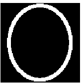
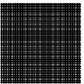
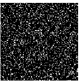
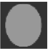
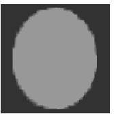
Before our discussion, perhaps we should first ask about what kind of sampling matrix $\boldsymbol{S}$ would work (or would not work). To answer this question, we consider an example shown in Figure 7. In Figure 7 we try to recover a simple disparity map consisting of an ellipse of constant intensity and a plain background. We consider three sampling patterns of approximately equal sampling ratios $\xi$: (a) a sampling pattern defined according to the magnitude of the disparity gradient; (b) an uniform grid with specified sampling ratio $\sqrt{\xi}$ along both directions; (c) a random sampling pattern drawn from an uniform distribution with probability $\xi$. The three sampling patterns correspondingly generate three sampled disparity maps. For each sampled disparity map, we run the proposed ADMM algorithm and record the reconstructed disparity map. In all experiments, we use a wavelet dictionary for demonstration.

Figure 7 suggests a strong message: For a fixed sampling budget $\xi$, one should pick samples along gradients. However, the pitfall is that this approach is not practical for two reasons. First, the gradient of the disparity map is not available prior to reconstructing the disparity. Therefore, all gradient information can only be inferred from the color image. Second, the gradients of a color image could be very different from the gradients of the corresponding disparity map. Thus, inferring the disparity gradient from the color image gradient is a challenging task. In the followings, we present a randomized sampling scheme to address these two issues.

We first consider an oracle situation where the gradients are assumed known. The goal is to see how much improvement one should expect to see.

Let $\boldsymbol{a}=[a_{1},\ldots,a_{N}]^{T}$ be a vector denoting the magnitude of the ground truth disparity map’s gradient. Given this oracle information about the disparity gradients, we consider a soft decision rule where a pixel is sampled with probability defined according to some function of $\{a_{j}\}_{j=1}^{N}$. Such a function is chosen based on the intuition that the sampled subset of gradients should carry the maximum amount of information compared to the full set of gradients. One way to capture this intuition is to require that the average gradient computed from all $N$ samples is similar to the average gradient computed from a subset of $\xi N$ samples.

To be more precise, we define the average gradient computed from all $N$ samples as

Similarly, we define the average gradient computed from a random subset of $\xi N$ samples as

where $\{I_{j}\}_{j=1}^{N}$ is a sequence of Bernoulli random variables with probability $\Pr[I_{j}=1]=p_{j}$. Here, the division of $a_{j}$ by $p_{j}$ is to ensure that $Y$ is unbiased, i.e., $\mathbb{E}[Y]=\mu$.

From (29) and (30), minimizing the difference between $Y$ and $\mu$ can be achieved by minimizing the variance $\mathbb{E}[(Y-\mu)^{2}]$. Moreover, we observe that

where the last equality holds because $\mathrm{Var}[I_{j}]=p_{j}(1-p_{j})$. Therefore, the optimal sampling probability $\{p_{j}\}_{j=1}^{N}$ can be found by solving the optimization problem

of which the solution is given by [50, Lemma 2]

where $\tau$ is the root of the equation

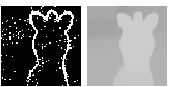
It is interesting to compare this new random sampling scheme versus a greedy sampling scheme by picking the $\xi N$ pixels with the largest gradients. Figure 8 shows the result. For the greedy sampling scheme, we first compute the gradient of the disparity map $\nabla\boldsymbol{x}\overset{\text{def}}{=}\sqrt{(\boldsymbol{D}_{x}\boldsymbol{x})^{2}+(\boldsymbol{D}_{y}\boldsymbol{x})^{2}}$ and threshold it to obtain a set of samples $\Omega\overset{\text{def}}{=}\{j\;|\;[\nabla\boldsymbol{x}]_{j}>\alpha\|\nabla\boldsymbol{x}\|_{\infty}\}$, where $\alpha=0.1$ is the threshold. The actual sampling ratio is then $|\Omega|/N$. For the randomized scheme, we let $\boldsymbol{a}=\nabla\boldsymbol{x}$ and we compute $p_{j}$ according to (31). In this particular example, we observe that the randomized sampling scheme achieves a PSNR improvement of more than 4 dB.

We now present a practically implementable sampling scheme. The challenge that we have to overcome is that the gradient information of the disparity is not available. Therefore, we propose the following two-stage sampling process.

Our proposed sampling scheme consists of two stages - a pilot stage to obtain a rough estimate of the disparity, and a refinement stage to improve the disparity estimate. In the first step pilot stage, we pick $\xi N/2$ samples (i.e., half of the desired number of samples) using an uniformly random sampling pattern. This gives a sampling pattern $\{I_{j}^{(1)}\}_{j=1}^{N}$, where the superscript denotes the first stage. Correspondingly, we have a sampling matrix $\boldsymbol{S}^{(1)}$ and the sampled data $\boldsymbol{b}^{(1)}$. Given $\boldsymbol{S}^{(1)}$ and $\boldsymbol{b}^{(1)}$, we apply the ADMM algorithm to obtain a pilot estimate $\boldsymbol{x}^{(1)}$.

In the second stage, we use the pilot estimate $\boldsymbol{x}^{(1)}$ as a guide to compute the gradient $\nabla\boldsymbol{x}^{(1)}$. By (31), this suggests that the optimal sampling probability is $p_{j}=\min(\tau[\nabla\boldsymbol{x}^{(1)}]_{j},1)$. However, in order to ensure that the $\xi N/2$ samples picked at the second stage do not overlap with those picked in the first stage, instead of letting $p_{j}=\min(\tau[\nabla\boldsymbol{x}^{(1)}]_{j},1)$, we let $p_{j}=\min(\tau a_{j},1)$, where

In words, $a_{j}$ defined by (33) forces $p_{j}=0$ when the $j$th pixel is picked in the first step. Thus, the non-zero entries of $\{I_{j}^{(1)}\}$ and $\{I_{j}^{(2)}\}$ are mutually exclusive, and hence we can now apply the ADMM algorithm to recover $\boldsymbol{x}^{(2)}$ from $\boldsymbol{S}_{1}+\boldsymbol{S}_{2}$ and $\boldsymbol{b}_{1}+\boldsymbol{b}_{2}$. The overall method is summarized in Algorithm 3.

The two-stage sampling procedure can be further improved by utilizing the prior information of the color image. The intuition is that since both color image and disparity map are captured from the same scene, strong gradients in the disparity map should align with those in the color image. However, since a color image typically contains complex gradients which are irrelevant to the disparity reconstruction, it is important to filter out these unwanted gradients while preserving the important ones. To this end, we consider the following patch-based principal component analysis.

Given a color image $\boldsymbol{y}\in\mathbb{R}^{N}$, we construct a collection of patches $\{\boldsymbol{y}_{j}\}_{j=1}^{N}$ where $\boldsymbol{y}_{j}\in\mathbb{R}^{d}$ denotes a vectorization of the $j$th patch of size $\sqrt{d}\times\sqrt{d}$ centered at pixel $j$ of the image. For patches centered at the corners or boundaries of the image, we apply a symmetrical padding to make sure that their sizes are $\sqrt{d}\times\sqrt{d}$. This will give us a total of $N$ patches.

Next, we form a data matrix $\boldsymbol{Y}\overset{\text{def}}{=}[\boldsymbol{y}_{1},\boldsymbol{y}_{2},\ldots,\boldsymbol{y}_{N}]$. This data matrix leads to a principal component decomposition as

where $\boldsymbol{U}$ is the eigenvector matrix, and $\boldsymbol{\Lambda}$ is the eigenvalue matrix. Geometrically, the projection of any patch $\boldsymbol{y}_{j}$ onto the subspace spanned by any eigenvector $\boldsymbol{u}_{i}$ is equivalent to applying a finite impulse response filter to the patch, i.e., $\boldsymbol{u}_{i}^{T}\boldsymbol{y}_{j}$. In many cases, except for the first eigenvector $\boldsymbol{u}_{1}$, all remaining eigenvectors $\boldsymbol{u}_{2},\ldots,\boldsymbol{u}_{d}$ are in the form of differential operators (of different orders and orientations, see examples in Figure 9). More interestingly, these filters are typically bandpass filters, which suggest that both low frequency components (e.g., smooth regions) and high frequency components (e.g., complex textures) of the color image can be filtered by applying the projections. Consequently, we consider the following filtered signal

where $d^{\prime}<d$ is a tunable parameter (which was set to $d^{\prime}=16$ for $d=49$ in this paper). Here, the absolute value in (35) is used to get the magnitude of $\langle\boldsymbol{u}_{i},\boldsymbol{y}_{j}\rangle$, as $a_{j}$ must be a non-negative number.

To see how this PCA concept can be incorporated into our two-stage sampling scheme, we make the following observations. First, the uniform sampling in Stage-1 can well be replaced by the PCA approach. In particular, instead of setting $I_{j}^{(1)}=1$ with probability $\xi/2$, we can define $a_{j}$ according to (35), and let $p_{j}=\min(\tau a_{j},1)$ for $\tau$ being the root of (32). Consequently, we let $I_{j}^{(1)}=1$ with probability $p_{j}$.

In Stage-2, since we have already had a pilot estimate of the disparity map, it is now possible to replace $\boldsymbol{Y}$ in (34) by a data matrix $\boldsymbol{X}=[\boldsymbol{x}_{1}^{(1)},\ldots,\boldsymbol{x}_{N}^{(1)}]$, where each $\boldsymbol{x}_{j}^{(1)}$ is a $d$-dimensional patch centered at the $j$th pixel of $\boldsymbol{x}^{(1)}$. Thus, instead of setting $a_{j}=[\nabla\boldsymbol{x}^{(1)}]_{j}$ in (33), we can set $a_{j}=\sum_{i=2}^{d^{\prime}}|\langle\boldsymbol{u}_{i},\boldsymbol{x}_{j}^{(1)}\rangle|$ using (35). The advantage of this new $a_{j}$ is that it softens the sampling probability at the object boundaries to a neighborhood surrounding the boundary. This reduces the risk of selecting irrelevant samples because of a bad pilot estimate.

As a comparison between sampling patterns, we consider a disparity map shown in Figure 10. Setting $\xi=0.1$ (i.e., 10%), we study four sampling patterns including two versions of our proposed two-stage method. We conduct a Monte-Carlo simulation by repeating 32 independent trials, and average the PSNRs. The results shown in Figure 10(c) are generated using the original two-stage sampling scheme without PCA improvement, whereas the results shown in Figure 10(d) are generated using an improved two-stage sampling scheme where the first stage is uniform and the second stage is PCA. These results indicate that for the same sampling ratio $\xi$, the choice of the sampling pattern has some strong influence to the reconstruction quality. For example, as compared to both uniform random sampling and grid sampling, the original two-stage sampling has about 2.44 dB improvement, and can be further improved by almost 3.76 dB using the PCA idea.

We first compare the proposed algorithm with existing methods on the Middlebury dataset¹¹ 1 http://vision.middlebury.edu/stereo/data/ where ground truth disparities are available. We consider two versions of the proposed algorithm: “Proposed WT+CT Grid” and “Proposed WT+CT 2-Stage”. “Proposed WT+CT Grid” is the ADMM algorithm presented in Section IV using both wavelet and contourlet bases. Here, “Grid” refers to using a deterministic uniform grid sampling pattern and “2-stage” refers to using the 2-stage randomized sampling scheme presented in Section V. We use Daubechies wavelet “db2” with 2 decomposition levels for wavelet dictionary, and we set “bior9-7” wavelet function with [5 6] directional decompositions for contourlet dictionary.

We also compare our method with [24], which has three differences from ours: (1) [24] uses a subgradient descent algorithm whereas we use an ADMM algorithm; (2) [24] considers only a wavelet basis whereas we consider a combined wavelet-contourlet basis; (3) [24] uses a combination of canny edges and uniformly random samples whereas we use a principled design process to determine samples.

In this experiment we do not compare with depth super resolution algorithms, e.g., [18, 51, 52]. These methods require a color image to guide the actual reconstruction process, which is different from what is presented here because we only use the color image for designing the sampling pattern. As a reference of these methods, we show the results of a bicubic interpolation using uniform grid sampling pattern.

Table II shows the PSNR values of various methods at different sampling ratios and sampling methods. It is clear that “Proposed WT+CT 2-Stage” outperforms the other methods by a significant margin. Moreover, as the sampling ratio increases, the PSNR gain of “Proposed WT+CT 2-Stage” is more prominent than that of other methods. For example, increasing from 5% to 25% for “Art”, “Proposed WT+CT 2-Stage” demonstrates an 18 dB PSNR improvement whereas bicubic only demonstrates 3 dB improvement.

It is also instructive to compare the percentage of bad pixels (% Bad Pixel), which is a popular metric to measure the quality of disparity estimates [53]. Given a threshold $\tau>0$, the percentage of bad pixels is defined as

where $\widehat{\boldsymbol{x}}$ is the reconstructed disparity and $\boldsymbol{x}^{*}$ is the ground truth disparity. Percentage of bad pixels can be considered as an absolute difference metric as compared to the mean squared metric of PSNR.

Table III shows the percentage of bad pixels of various methods at different sampling ratios and sampling methods. The results indicate that “Proposed WT+CT 2-Stage” has a relatively higher % Bad Pixel at $\tau=1$ than other methods, but has a lower % Bad Pixel at $\tau=2$ and $\tau=3$. This result suggests that most of the errors of “Proposed WT+CT 2-Stage” are small and there are very few outliers. In contrast, bicubic grid (for example) has a low % Bad Pixel at $\tau=1$ but high % Bad Pixel at $\tau=2$ and $\tau=3$. This implies that a significant portion of the bicubic results has large error. Intuitively, the results suggest that in the bicubic case, some strong edges and corners are completely missed, whereas these information are kept in “Proposed WT+CT 2-Stage”.

Finally, we show the performance of the proposed algorithm towards additive i.i.d. Gaussian noise. The purpose of this experiment is to demonstrate the sensitivity and robustness of the algorithm in the presence of noise. While in reality the noise in disparity estimates is not i.i.d. Gaussian, the result presented here serves as a reference for the algorithm’s performance. A more realistic experiment on real data will be illustrated in the next subsection.

The results are shown in Figure 11. Using “Bicubic Grid” as the baseline, we observe that “Proposed WT+CT 2-Stage” on average has 5.79 dB improvement, “Proposed WT+CT Grid” has 3.60 dB improvement, whereas “[24] Grid” has only 3.02 dB improvement. This provides a good indicator of the robustness of the proposed methods.

References

- [1] M. A. Lefsky, W. B. Cohen, G. G. Parker, and D. J. Harding, “LIDAR remote sensing of above-ground biomass in three biomes,” Global Ecology and Biogeography, vol. 11, pp. 393–399, Oct. 2002.
- [2] S. Agarwal, N. Snavely, I. Simon, S.M. Seitz, and R. Szeliski, “Building Rome in a day,” in Proc. IEEE Int. Conf. Computer Vision (ICCV’09), Sep. 2009, pp. 72–79.
- [3] S. Burion, “Human detection for robotic urban search and rescue,” M.S. thesis, Carnegie Mellon Univ., 2004, available at http://www.cs.cmu.edu/afs/cs/project/retsina-31/www/Report/Final%20Report.pdf.
- [4] R. Khoshabeh, J. Juang, M.A. Talamini, and T.Q. Nguyen, “Multiview glasses-free 3-D laparoscopy,” IEEE Trans. Bio. Eng., vol. 59, no. 10, pp. 2859–2865, Oct. 2012.
- [5] S. H. Chan, R. Khoshabeh, K. B. Gibson, P. E. Gill, and T. Q. Nguyen, “An augmented Lagrangian method for total variation video restoration,” IEEE Trans. Image Process., vol. 20, no. 11, pp. 3097–3111, Nov. 2011.
- [6] S. Foix, G. Alenya, and C. Torras, “Lock-in time-of-flight (ToF) cameras: A survey,” IEEE Sensors Journal, vol. 11, no. 9, pp. 1917–1926, Sep. 2011.
- [7] B. Schwarz, “LIDAR: Mapping the world in 3D,” Nature Photonics, vol. 4, pp. 429–430, Jul. 2010.
- [8] C. Niclass, M. Soga, H. Matsubara, S. Kato, and M. Kagami, “A 100-m range 10-frame/s 340 96-pixel time-of-flight depth sensor in 0.18- cmos,” IEEE Journal of Solid-State Circuits, vol. 48, no. 2, pp. 559–572, Feb. 2013.
- [9] X. Mei, X. Sun, M. Zhou, S. Jiao, H. Wang, and X. Zhang, “On building an accurate stereo matching system on graphics hardware,” in Proc. IEEE Int. Conf. Computer Vision (ICCV’11), Nov. 2011, pp. 467–474.
- [10] A. Klaus, M. Sormann, and K. Karner, “Segment-based stereo matching using belief propagation and a self-adapting dissimilarity measure,” in Proc. IEEE Int. Conf. on Pattern Recognition (ICPR’06), Aug. 2006, vol. 3, pp. 15–18.
- [11] Z. Wang and Z. Zheng, “A region based stereo matching algorithm using cooperative optimization,” in Proc. IEEE Int. Conf. Computer Vision and Pattern Recognition (CVPR’08), Jun. 2008, pp. 1–8.
- [12] Q. Yang, L. Wang, R. Yang, H. Stewenius, and D. Nister, “Stereo matching with color-weighted correlation, hierarchical belief propagation, and occlusion handling,” IEEE Trans. Pattern Anal. Machine Intell., vol. 31, no. 3, pp. 492–504, Mar. 2009.
- [13] J. Heikkila and O. Silven, “A four-step camera calibration procedure with implicit image correction,” in in Proc. IEEE Int. Conf. Computer Vision and Pattern Recognition (CVPR’97), Jun. 1997, pp. 1106–1112.
- [14] Z. Zhang, “Flexible camera calibration by viewing a plane from unknown orientations,” in Proc. IEEE Int. Conf. Computer Vision (ICCV’99), Sep. 1999, vol. 1, pp. 666–673.
- [15] R. S. Feris, J. Gemmell, K. Toyama, and V. Kruger, “Hierarchical wavelet networks for facial feature localization,” in Proc. IEEE Int. Conf. Automatic Face and Gesture Recognition (FG’02), May 2002, pp. 118–123.
- [16] Y. Ke and R. Sukthankar, “PCA-SIFT: A more distinctive representation for local image descriptors,” in Proc. IEEE Int. Conf. Computer Vision and Pattern Recognition (CVPR’04), Jun. 2004, vol. 2, pp. 506–513.
- [17] J. Diebel and S. Thrun, “An application of Markov random field to range sensing,” in Advances in Neural Info. Process. System (NIPS’05), Dec. 2005, pp. 291–298.
- [18] Q. Yang, R. Yang, J. Davis, and D. Nister, “Spatial-depth super resolution for range images,” in Proc. IEEE Int. Conf. Computer Vision and Pattern Recognition (CVPR’07), Jun. 2007, pp. 1–8.
- [19] J. Li, T. Xue, L. Sun, and J. Liu, “Joint example-based depth map super-resolution,” in IEEE Int. Conf. Multimedia and Expo (ICME’12), Jul. 2012, pp. 152–157.
- [20] O. M. Aodha, N. D. F. Campbell, A. Nair, and G. J. Brostow, “Patch based synthesis for single depth image super-resolution,” in Proc. European Conf. Computer Vision (ECCV’12), Oct. 2012, pp. 71–84.
- [21] E. J. Candès and M. B. Wakin, “An introduction to compressive sampling,” IEEE Signal Process. Magazine, vol. 25, no. 2, pp. 21–30, Mar. 2008.
- [22] D. L. Donoho and X. Huo, “Uncertainty principles and ideal atomic decomposition,” IEEE Trans. Info. Theory, vol. 47, no. 7, pp. 2845–2862, Nov. 2001.
- [23] M. Elad and A. M. Bruckstein, “A generalized uncertainty principle and sparse representation in pairs of bases,” IEEE Trans. Info. Theory, vol. 48, no. 9, pp. 2558–2567, Sep. 2002.
- [24] S. Hawe, M. Kleinsteuber, and K. Diepold, “Dense disparity maps from sparse disparity measurements,” in Proc. IEEE Int. Conf. Computer Vision (ICCV’11), Nov. 2011, pp. 2126–2133.
- [25] S. Schwartz, A. Wong, and D. A. Clausi, “Saliency-guided compressive sensing approach to efficient laser range measurement,” J. Vis. Commun. Image R., vol. 24, no. 2, pp. 160–170, 2013.
- [26] S. Schwartz, A. Wong, and D. A. Clausi, “Multi-scale saliency-guided compressive sensing approach to efficient robotic laser range measurement,” in Proc. IEEE Computer Society Conf. Computer, Robot Vision, 2012, pp. 1–8.
- [27] A. Kirmani, A. Colaco, F.N.C. Wong, and V.K. Goyal, “CODAC: A compressive depth acquisition camera framework,” in Proc. IEEE Int. Conf. Acoust., Speech, and Signal Process. (ICASSP’12), Mar. 2012, pp. 5425–5428.
- [28] A. Kirmani, D. Venkatraman, D. Shin, A. Colaco, F.N. C. Wong, J.H. Shapiro, and V.K. Goyal, “First photon imaging,” Science Magazine, vol. 343, no. 6166, pp. 58–61, Nov. 2013.
- [29] R. I. Hartley and A. Zisserman, Multiple View Geometry in Computer Vision, Cambridge University Press, Mar. 2004.
- [30] F. Chung and L. Lu, “Concentration inequalities and martingale inequalities: a survey,” Internet Mathematics, vol. 3, no. 1, pp. 79–127, 2006.
- [31] M. N. Do and M. Vetterli, “The contourlet transform: An efficient directional multiresolution image representation,” IEEE Trans. Image Process., vol. 14, no. 12, pp. 2091–2106, Dec. 2005.
- [32] M. Elad, P. Milanfar, and R. Rubinstein, “Analysis versus synthesis in signal priors,” Inverse Problems, vol. 23, pp. 947–968, Apr. 2007.
- [33] E. J. Candès and Y. Plan, “A probabilistic and RIPless theory of compressed sensing,” IEEE Trans. Information Theory, vol. 57, no. 11, pp. 7235–7254, Nov. 2011.
- [34] R. Baraniuk, M. Davenport, R. DeVore, and M. Wakin, “A simple proof of the restricted isometry property for random matrices,” Const. Approx., vol. 28, no. 3, pp. 253–263, Dec. 2008.
- [35] M. Aharon, M. Elad, and A. Bruckstein, “K-SVD: An algorithm for designing overcomplete dictionaries for sparse representation,” IEEE Trans. Signal Process., vol. 54, no. 11, pp. 4311–4322, Nov. 2006.
- [36] J. Mairal, M. Elad, and G. Sapiro, “Sparse representation for color image restoration,” IEEE Trans. Image Process., vol. 17, no. 1, pp. 53–69, Jan. 2008.
- [37] S. Mallat, A Wavelet Tour of Signal Processing: The Sparse Way, Academic Press, Dec. 2008.
- [38] D. D. Y. Po and M. N. Do, “Directional multiscale modeling of images using the contourlet transform,” IEEE Trans. Image Process., vol. 15, no. 6, pp. 1610–1620, Jun. 2006.
- [39] E. J. Candès and D. L. Donoho, “Recovering edges in ill-posed inverse problems: Optimality of curvelet frames,” Annals of Statistics, , no. 3, pp. 784–842, Aug. 2002.
- [40] E. J. Candès and D. L. Donoho, “New tight frames of curvelets and optimal representations of objects with piecewise singularities,” Communications on Pure and Applied Mathematics, vol. 57, no. 2, pp. 219–266, Feb. 2004.
- [41] E. Le Pennec and S. Mallat, “Bandelet image approximation and compression,” Multiscale Model. Simul., vol. 4, no. 3, pp. 992–1039, 2005.
- [42] M. Vetterli and J. Kovačević, Wavelets and subband coding, Prentice Hall, 1995.
- [43] J. J. Moreau, “Proximité et dualtité danes un espace hilbertien,” Bulletin de la Société Mathématique de France, vol. 93, pp. 273–299, 1965.
- [44] J. Eckstein and D. P. Bertsekas, “On the Douglas-Rachford splitting method and the proximal point algorithm for maximal monotone operators,” Math. Program., vol. 55, no. 3, pp. 293–318, Jun. 1992.
- [45] J. Yang, Y. Zhang, and W. Yin, “An efficient TVL1 algorithm for deblurring multichannel images corrupted by impulsive noise,” SIAM J. on Sci. Comput., vol. 31, no. 4, pp. 2842–2865, Jul. 2009.
- [46] D. Han and X. Yuan, “A note on the alternating direction method of multipliers,” J. of Optim. Theory and Applications, vol. 155, no. 1, pp. 227–238, Oct. 2012.
- [47] S. Boyd, N. Parikh, E. Chu, B. Peleato, and J. Eckstein, “Distributed optimization and statistical learning via the alternating direction method of multipliers,” Found. Trends Mach. Learn., vol. 3, no. 1, pp. 1–122, Jan. 2011.
- [48] W. Dai and O. Milenkovic, “Subspace pursuit for compressive sensing signal reconstruction,” IEEE Trans. Info. Theory, vol. 55, no. 5, pp. 2230–2249, May 2009.
- [49] L. Liu, S. H. Chan, and T. Q. Nguyen, “Depth reconstruction from sparse samples: Representation, algorithm, and sampling (supplementary material),” Available online at http://arxiv.org/abs/1407.3840.
- [50] S. H. Chan, T. Zickler, and Y. M. Lu, “Monte Carlo non-local means: Random sampling for large-scale image filtering,” IEEE Trans. Image Process., vol. 23, no. 8, pp. 3711–3725, Aug. 2014.
- [51] F. Li, J. Yu, and J. Chai, “A hybrid camera for motion deblurring and depth map super-resolution,” in Proc. IEEE Int. Conf. Computer Vision and Pattern Recognition (CVPR’08), Jun. 2008, pp. 1–8.
- [52] J. Park, H. Kim, Y. Tai, M.S. Brown, and I. Kweon, “High quality depth map upsampling for 3D-TOF cameras,” in Proc. IEEE Int. Conf. Computer Vision (ICCV’11), Nov. 2011, pp. 1623–1630.
- [53] D. Scharstein and R. Szeliski, “A taxonomy and evaluation of dense two-frame stereo correspondence algorithms,” Int. J. on Computer Vision, vol. 47, no. 1-3, pp. 7–42, Apr. 2002.
- [54] Z. Lee, J. Juang, and T. Q. Nguyen, “Local disparity estimation with three-moded cross census and advanced support weight,” IEEE Trans. Multimedia, vol. 15, no. 8, pp. 1855–1864, Dec. 2013.