跳到论文正文
W Papers独立论文阅读器 arXiv:1407.3574 论文正文 计算阅读时间 · 0%
引用这篇论文根据当前论文元数据生成,正式投稿前建议核对。


License: arXiv.org perpetual non-exclusive license
arXiv:1407.3574v3 [hep-ph] 30 Sep 2014

9 September, 2014 OU-HET 807, KIAS-P14008

Dark matter

in the SO(5)×\timesU(1) gauge-Higgs unification

Shuichiro Funatsu∗, Hisaki Hatanaka†, Yutaka Hosotani∗
Yuta Orikasa†,‡ and Takuya Shimotani∗

∗Department of Physics, Osaka University, Toyonaka, Osaka 560-0043, Japan

†School of Physics, KIAS, Seoul 130-722, Republic of Korea

and

‡Department of Physics and Astronomy, Seoul National University,
Seoul 151-742, Republic of Korea

Abstract

In the S​O​(5)×U⁡(1)SO(5)\times U(1) gauge-Higgs unification the lightest, neutral component of nFn_{F} S​O​(5)SO(5)-spinor fermions (dark fermions), which are relevant for having the observed unstable Higgs boson, becomes the dark matter of the universe. We show that the relic abundance of the dark matter determined by WMAP and Planck data is reproduced, below the bound placed by the direct detection experiment by LUX, by a model with one light and three heavier (nF=4n_{F}=4) dark fermions with the lightest one of a mass from 2.3 TeV to 3.1 TeV. The corresponding Aharonov-Bohm phase θH\theta_{H} in the fifth dimension ranges from 0.097 to 0.074. The case of nF=3n_{F}=3 (nF=5,6n_{F}=5,6) dark fermions yields the relic abundance smaller (larger) than the observed limit.

1 Introduction

The Higgs boson of a mass around 125.5 GeV was discovered at LHC.[1, 2] It is not clear, however, whether or not the particle discovered is precisely the Higgs boson specified in the standard model (SM). Physics beyond the standard model may be hiding, showing up at the upgraded LHC. Couplings of the Higgs boson to other particles may slightly deviate from those in SM, and new particles may be produced, say, in the 4 - 7 TeV range. SM lacks a principle governing dynamics of the Higgs boson. Further SM has no clue to explain the dark matter (DM) in the universe.

In the gauge-Higgs unification (GHU) the Higgs boson is unified with gauge bosons. The 4D Higgs boson appears as a part of the extra-dimensional component of gauge fields so that its dynamics are governed by the gauge principle.[3]-[8] It has been shown that in the S​O​(5)×U⁡(1)SO(5)\times U(1) GHU in the Randall-Sundrum warped space the low energy physics appears almost the same as that in SM, consistent with all LHC data.[9]-[16] Contributions of Kaluza-Klein (KK) excited modes to the H→γ​γH\rightarrow\gamma\gamma decay, for example, turn out very small.[15] Higgs couplings to gauge bosons, quarks and leptons at the tree level are suppressed by a common factor cos⁡θH\cos\theta_{H} where θH\theta_{H} is the Aharonov-Bohm phase in the extra dimension.[17]-[22] All of the precision measurements, the tree-unitary constraint, and the Z′Z^{\prime} search indicate that θH<0.2\theta_{H}<0.2.[9, 23] The S​O​(5)×U⁡(1)SO(5)\times U(1) GHU predicts new structure at higher energies. The masses of the 1st KK modes of ZZ and γ\gamma are predicted to be 3∼73\sim 7\,TeV for θH=0.1∼0.2\theta_{H}=0.1\sim 0.2. The Higgs cubic and quartic self-coupling should be smaller than those in the SM by 10% - 20%.[16] Many other signals of GHU have been investigated.[24]-[33]

Another important issue is the dark matter.[34] Supersymmetric theory, the leading model of physics beyond the SM, predicts the lightest supersymmetric particle as a dark matter candidate.[35, 36] The lightest KK particle in universal extra dimension models [37]-[42], the lightest T-odd particle in the little Higgs models [43, 44], a fermionic composite state in the composite Higgs models [45]-[47], and axions [48]-[52] can be identified as dark matter. In the Higgs portal scenario the Higgs boson couples to dark matter in the hidden sector [53]-[57], and the dynamical dark matter scenario has been proposed.[58] Is there a dark matter candidate in the S​O​(5)×U⁡(1)SO(5)\times U(1) gauge-Higgs unification model? Can it explain the relic abundance reduced from the WMAP/Planck data and other observations, within the constraints from direct detection searches? A few scenarios for dark matter in GHU have been proposed.[59, 60, 61, 62] In this paper we would like to show that the realistic S​O​(5)×U⁡(1)SO(5)\times U(1) gauge-Higgs unification model contains a natural candidate for dark matter.

In the minimal S​O​(5)×U⁡(1)SO(5)\times U(1) gauge-Higgs unification model, in which only quark-lepton vector multiplets and associated brane fermions are introduced in the fermion sector, the effective potential is minimized at θH=12​π\theta_{H}=\hbox{$\frac{1}{2}$}\pi, which in turn implies that the Higgs boson becomes stable, contradicting with the observation.[11, 13, 61] To have an unstable Higgs boson, it is necessary to introduce fermion multiplets in the spinor representation of S​O​(5)SO(5) which do not appear at low energies.[15] Indeed, the presence of these fermions, with the gauge fields and top quark multiplet, naturally leads to 0<θH<12​π0<\theta_{H}<\hbox{$\frac{1}{2}$}\pi, yielding predictions consistent with the observation. One remarkable property is that independent of the details of these S​O​(5)SO(5)-spinor fermions there appears the universality relations among θH\theta_{H}, the masses of KK ZZ/photon, and the Higgs self couplings.

We show that the lightest, neutral component of the S​O​(5)SO(5)-spinor fermions is absolutely stable, and becomes the dark matter of the universe. For this reason the S​O​(5)SO(5)-spinor fermion is called as a dark fermion in the present paper. It is heavy with a mass around 2∼42\sim 4\,TeV, but its couplings to the Higgs boson are small. From its relic abundance the number and structure of the dark fermion multiplets are inferred. It is curious that the Higgs dynamics are intimately related to the dark matter in the gauge-Higgs unification.

The paper is organized as follows. In Section 2 the S​O​(5)×U⁡(1)SO(5)\times U(1) model is introduced. In Section 3 it is shown that the neutral components of dark fermions become the dark matter, and the relic abundance is evaluated. In Section 4 the spin-independent cross section of the dark matter candidate with nucleons is evaluated, and the compatibility with the constraint coming from the direct detection experiments, XENON100 and LUX [63, 64], is examined. It will be found that the model with nF=4n_{F}=4 nondegenerate dark fermions with the lightest one of a mass 2.3 TeV∼\sim3.1 TeV explains the relic abundance of the dark matter determined from the WMAP/Planck data below the bound placed by the direct detection observation of LUX. Section 5 is devoted to the conclusion and discussions. In the appendices wave functions and couplings of dark fermions and relevant gauge bosons are summarized.

2 Model

The model of the S​O​(5)×U⁡(1)SO(5)\times U(1) GHU is defined in the Randall-Sundrum (RS) warped space with a metric

d​s2=GM​N​d​xM​d​xN=e−2​σ​(y)​ημ​ν​d​xμ​d​xν+d​y2,ds^{2}=G_{MN}dx^{M}dx^{N}=e^{-2\sigma(y)}\eta_{\mu\nu}dx^{\mu}dx^{\nu}+dy^{2}, (2.1)

where ημ​ν=diag​(−1,1,1,1)\eta_{\mu\nu}=\text{diag}(-1,1,1,1), σ⁡(y)=σ⁡(y+2​L)=σ⁡(−y)\sigma(y)=\sigma(y+2L)=\sigma(-y), and σ⁡(y)=k​|y|\sigma(y)=k|y| for |y|≤L|y|\leq L. The Planck and TeV branes are located at y=0y=0 and y=Ly=L, respectively. The bulk region 0<y<L0<y<L is anti-de Sitter (AdS) spacetime with a cosmological constant Λ=−6​k2\Lambda=-6k^{2}. The warp factor zL≡ek​Lz_{L}\equiv e^{kL} is large, zL≫1z_{L}\gg 1, and the Kaluza-Klein mass scale is given by mK​K=π​k/(zL−1)∼π​k​zL−1m_{KK}=\pi k/(z_{L}-1)\sim\pi kz_{L}^{-1}.

The model consists of S​O​(5)×U​(1)XSO(5)\times U(1)_{X} gauge fields (AM,BM)(A_{M},B_{M}), quark-lepton multiplets Ψa\Psi_{a}, S​O​(5)SO(5)-spinor fermions (dark fermions) ΨFi\Psi_{F_{i}}, brane fermions χ^α​R\hat{\chi}_{\alpha R}, and brane scalar Φ^\hat{\Phi}.[12, 15] The bulk part of the action is given by

Sbulk=∫d5x−G[−tr(1 4F(A)​M​NFM​N(A)+12​ξ(fgf(A))2+ℒgh(A))\displaystyle\hskip-28.45274ptS_{\text{bulk}}=\int d^{5}x\sqrt{-G}\,\Bigl[-{\rm tr\,}\Bigl(\frac{1}{\;4\;}F^{(A)MN}F^{(A)}_{MN}+\frac{1}{2\xi}(f^{(A)}_{\text{gf}})^{2}+\mathcal{L}^{(A)}_{\text{gh}}\Bigr) (2.2)
−(1 4​F(B)​M​N​FM​N(B)+12​ξ​(fgf(B))2+ℒgh(B))\displaystyle\hskip 71.13188pt-\Bigl(\frac{1}{\;4\;}F^{(B)MN}F^{(B)}_{MN}+\frac{1}{2\xi}(f^{(B)}_{\text{gf}})^{2}+\mathcal{L}^{(B)}_{\text{gh}}\Bigr) (2.3)
+∑aΨ¯a𝒟(ca)Ψa+∑i=1nFΨ¯Fi𝒟(cFi)ΨFi],\displaystyle\hskip 71.13188pt+\sum_{a}\bar{\Psi}_{a}\mathcal{D}(c_{a})\Psi_{a}+\sum_{i=1}^{n_{F}}\bar{\Psi}_{F_{i}}\mathcal{D}(c_{F_{i}})\Psi_{F_{i}}\Bigr], (2.4)
𝒟(c)=ΓAeAM(∂M+18ωM​B​C[ΓB,ΓC]−igAAM−igBQXBM)−cσ′(y).\displaystyle\hskip-28.45274pt\mathcal{D}(c)=\Gamma^{A}{e_{A}}^{M}\Big(\partial_{M}+\frac{1}{8}\omega_{MBC}[\Gamma^{B},\Gamma^{C}]-ig_{A}A_{M}-ig_{B}Q_{X}B_{M}\Big)-c\sigma^{\prime}(y). (2.5)

The gauge fixing and ghost terms are denoted as functionals with subscripts gf and gh, respectively. FM​N(A)=∂MAN−∂NAM−i​gA​[AM,AN]F^{(A)}_{MN}=\partial_{M}A_{N}-\partial_{N}A_{M}-ig_{A}\bigl[A_{M},A_{N}\bigr], and FM​N(B)=∂MBN−∂NBMF^{(B)}_{MN}=\partial_{M}B_{N}-\partial_{N}B_{M}. The color S​U​(3)CSU(3)_{C} gluon fields and their interactions have been suppressed in the present paper. The S​O​(5)SO(5) gauge fields AMA_{M} are decomposed as

AM=∑aL=13AMaL​TaL+∑aR=13AMaR​TaR+∑a^=14AMa^​Ta^,A_{M}=\sum^{3}_{a_{L}=1}A_{M}^{a_{L}}T^{a_{L}}+\sum^{3}_{a_{R}=1}A_{M}^{a_{R}}T^{a_{R}}+\sum^{4}_{\hat{a}=1}A_{M}^{\hat{a}}T^{\hat{a}}, (2.6)

where TaL,aR​(aL,aR=1,2,3)T^{a_{L},a_{R}}(a_{L},a_{R}=1,2,3) and Ta^​(a^=1,2,3,4)T^{\hat{a}}(\hat{a}=1,2,3,4) are the generators of S​O​(4)≃S​U​(2)L×S​U​(2)RSO(4)\simeq SU(2)_{L}\times SU(2)_{R} and S​O​(5)/S​O​(4)SO(5)/SO(4), respectively.

In the fermion part Ψ¯=i​Ψ†​Γ0\bar{\Psi}=i\Psi^{\dagger}\Gamma^{0} and ΓM\Gamma^{M} matrices are given by

Γμ=γμ=(σμσ¯μ),Γ5=γ5=(1−1),\displaystyle\hskip-28.45274pt\Gamma^{\mu}=\gamma^{\mu}=\begin{pmatrix}&\sigma^{\mu}\cr\bar{\sigma}^{\mu}&\end{pmatrix}~,~~\Gamma^{5}=\gamma^{5}=\begin{pmatrix}1&\cr&-1\end{pmatrix}~, (2.7)
σμ=(1,σ→),σ¯μ=(−1,σ→).\displaystyle\hskip-28.45274pt\sigma^{\mu}=(1,\,\vec{\sigma})~,~~\bar{\sigma}^{\mu}=(-1,\,\vec{\sigma})~. (2.8)

The quark-lepton multiplets Ψa\Psi_{a} are introduced in the vector representation of S​O​(5)SO(5). In contrast, nFn_{F} dark fermions ΨFi\Psi_{F_{i}} are introduced in the spinor representation. The cc term in Eq. (2.5) gives a bulk kink mass, where σ′​(y)=k​ϵ​(y)\sigma^{\prime}(y)=k\epsilon(y) is a periodic step function with a magnitude kk. The dimensionless parameter cc plays an important role in controlling profiles of fermion wave functions.

The orbifold boundary conditions at y0=0y_{0}=0 and y1=Ly_{1}=L are given by

(AμAy)⁡(x,yj−y)=Pvec​(Aμ−Ay)​(x,yj+y)​Pvec−1,\displaystyle\hskip-28.45274pt\begin{pmatrix}A_{\mu}\\ A_{y}\end{pmatrix}(x,y_{j}-y)=P_{{\rm vec}}\begin{pmatrix}A_{\mu}\\ -A_{y}\end{pmatrix}(x,y_{j}+y)P_{{\rm vec}}^{-1}, (2.9)
(BμBy)⁡(x,yj−y)=(Bμ−By)⁡(x,yj+y),\displaystyle\hskip-28.45274pt\begin{pmatrix}B_{\mu}\\ B_{y}\end{pmatrix}(x,y_{j}-y)=\begin{pmatrix}B_{\mu}\\ -B_{y}\end{pmatrix}(x,y_{j}+y), (2.10)
Ψa​(x,yj−y)=Pvec​Γ5​Ψa​(x,yj+y),\displaystyle\hskip-28.45274pt\Psi_{a}(x,y_{j}-y)=P_{{\rm vec}}\Gamma^{5}\Psi_{a}(x,y_{j}+y), (2.11)
ΨFi​(x,yj−y)=ηFi​(−1)j​Psp​Γ5​ΨFi​(x,yj+y),ηFi=±1,\displaystyle\hskip-28.45274pt\Psi_{F_{i}}(x,y_{j}-y)=\eta_{F_{i}}(-1)^{j}P_{{\rm sp}}\Gamma^{5}\Psi_{F_{i}}(x,y_{j}+y),~~~\eta_{F_{i}}=\pm 1, (2.12)
Pvec=diag​(−1,−1,−1,−1,+1),Psp=diag​(+1,+1,−1,−1).\displaystyle\hskip-28.45274ptP_{{\rm vec}}=\text{diag}\,(-1,-1,-1,-1,+1),\quad P_{{\rm sp}}=\text{diag}\,(+1,+1,-1,-1). (2.13)

The S​O​(5)×U​(1)XSO(5)\times U(1)_{X} symmetry is reduced to S​O​(4)×U​(1)X≃S​U​(2)L×S​U​(2)R×U​(1)XSO(4)\times U(1)_{X}\simeq SU(2)_{L}\times SU(2)_{R}\times U(1)_{X} by the orbifold boundary conditions. Various orbifold boundary conditions fall into a finite number of equivalence classes of boundary conditions.[65, 66] The physical symmetry of the true vacuum in each equivalence class of boundary conditions is dynamically determined at the quantum level by the Hosotani mechanism. Recently dynamics for selecting boundary conditions have been proposed as well.[67] The Hosotani mechanism has been explored and established, not only in perturbation theory, but also on the lattice nonperturbatively.[68]

The brane action SbraneS_{\rm brane} contains brane fermions χ^α​R​(x)\hat{\chi}_{\alpha R}(x), brane scalar Φ^​(x)\hat{\Phi}(x), Aμ​(x,y=0)A_{\mu}(x,y=0) and Ψa​(x,y=0)\Psi_{a}(x,y=0). It manifestly preserves gauge-invariance in S​O​(4)×U​(1)XSO(4)\times U(1)_{X}. Φ^\hat{\Phi} develops non-vanishing expectation value ⟨​Φ^​⟩≫mKK\raise 0.68889pt\hbox{$\langle$}\lower 0.68889pt\hbox{}\hat{\Phi}\raise 0.68889pt\hbox{$\rangle$}\lower 0.68889pt\hbox{}\gg m_{\rm KK}, which results in spontaneous breaking of S​O​(4)×U​(1)XSO(4)\times U(1)_{X} into S​U​(2)L×U​(1)YSU(2)_{L}\times U(1)_{Y} and in making all exotic fermions heavy.

The 4D Higgs field, which is a bidoublet in S​U​(2)L×S​U​(2)RSU(2)_{L}\times SU(2)_{R}, appears as a zero mode in the S​O​(5)/S​O​(4)SO(5)/SO(4) part of the fifth dimensional component of the vector potential Aya^​(x,y)A^{\hat{a}}_{y}(x,y) with custodial symmetry.[9, 69, 70] Without loss of generality one can set ⟨Aya^⟩∝δa​4\langle A^{\hat{a}}_{y}\rangle\propto\delta^{a4} when the EW symmetry is spontaneously broken. The zero modes of Aya^A^{\hat{a}}_{y} (a = 1,2,3) are absorbed by WW and ZZ bosons. The 4D neutral Higgs field H⁡(x)H(x) is a fluctuation mode of the Wilson line phase θH\theta_{H} which is an Aharonov-Bohm phase in the fifth dimension;

Ay4^​(x,y)={θH​fH+H⁡(x)}​uH​(y)+⋯,\displaystyle\hskip-28.45274ptA^{\hat{4}}_{y}(x,y)=\big\{\theta_{H}f_{H}+H(x)\big\}u_{H}(y)+\cdots~, (2.14)
exp⁡{i2​θH⋅2​2​T4^}=exp⁡{i​gA​∫0Ld​y​⟨​Ay​⟩},\displaystyle\hskip-28.45274pt\exp\Big\{\frac{i}{2}\theta_{H}\cdot 2\sqrt{2}T^{\hat{4}}\Big\}=\exp\bigg\{ig_{A}\int^{L}_{0}dy\raise 0.68889pt\hbox{$\langle$}\lower 0.68889pt\hbox{}A_{y}\raise 0.68889pt\hbox{$\rangle$}\lower 0.68889pt\hbox{}\bigg\}~, (2.15)
fH=2gA​kzL2−1=2gw​kL⁡(zL2−1).\displaystyle\hskip-28.45274ptf_{H}=\frac{2}{g_{A}}\sqrt{\frac{k}{z_{L}^{2}-1}}=\frac{2}{g_{w}}\sqrt{\frac{k}{L(z_{L}^{2}-1)}}~. (2.16)

Here the wave function of the 4D Higgs boson is given by uH​(y)=[2​k/(zL2−1)]1/2​e2​k​yu_{H}(y)=[2k/(z_{L}^{2}-1)]^{1/2}e^{2ky} for 0≤y≤L0\leq y\leq L and uH​(−y)=uH​(y)=uH​(y+2​L)u_{H}(-y)=u_{H}(y)=u_{H}(y+2L). gw=gA/Lg_{w}=g_{A}/\sqrt{L} is the dimensionless 4D S​U​(2)LSU(2)_{L} coupling.

For each generation two vector multiplets Ψ1\Psi_{1} and Ψ2\Psi_{2} for quarks and two vector multiplets Ψ3\Psi_{3} and Ψ4\Psi_{4} for leptons are introduced. In contrast, the dark fermion ΨFi\Psi_{F_{i}} belongs to the spinor representation of S​O​(5)SO(5), having four components

ΨFi=(ψl​1iψl​2iψr​1iψr​2i).\Psi_{F_{i}}=\begin{pmatrix}\psi^{i}_{l1}\\ \psi^{i}_{l2}\\ \psi^{i}_{r1}\\ \psi^{i}_{r2}\end{pmatrix}. (2.17)

ψli\psi^{i}_{l} and ψri\psi^{i}_{r} are S​U​(2)LSU(2)_{L} and S​U​(2)RSU(2)_{R} doublets, respectively. They mix with each other for θH≠0\theta_{H}\not=0. The electric charge is given by QEM=T3L+T3R+QXQ_{\rm EM}=T^{3_{L}}+T^{3_{R}}+Q_{X}. We take QX=12Q_{X}=\hbox{$\frac{1}{2}$} for ΨFi\Psi_{F_{i}} so that it contains charge 1 and 0 components.

The KK decomposition of ΨFi\Psi_{F_{i}} fields are summarized in Appendix B. With the boundary condition (2.13) ΨFi​(x,z)\Psi_{F_{i}}(x,z) does not have zero modes, and is expanded in the KK modes Fi+(n)​(x)F^{+(n)}_{i}(x) and Fi0​(n)​(x)F^{0(n)}_{i}(x) (n=1,2,3,⋯n=1,2,3,\cdots) as in (B.4). The mass spectrum is determined by (B.17). With ηFi=+1\eta_{F_{i}}=+1 in the boundary condition for ΨFi\Psi_{F_{i}} in (2.13) and for small θH\theta_{H} the odd KK number modes Fi+(n),Fi0​(n)F^{+(n)}_{i},F^{0(n)}_{i} (nn: odd) are mostly S​U​(2)RSU(2)_{R} doublets, containing S​U​(2)LSU(2)_{L} components slightly. The even KK number modes Fi+(n),Fi0​(n)F^{+(n)}_{i},F^{0(n)}_{i} (nn: even) are mostly S​U​(2)LSU(2)_{L} doublets. Consequenltly the first KK modes Fi+(1),Fi0​(1)F^{+(1)}_{i},F^{0(1)}_{i} couple to the S​U​(2)LSU(2)_{L} gauge bosons (WW and ZZ) very weakly. On the other hand, with ηFi=−1\eta_{F_{i}}=-1, Fi+(n),Fi0​(n)F^{+(n)}_{i},F^{0(n)}_{i} (nn: odd) are mostly S​U​(2)LSU(2)_{L} doublets, and the first KK modes Fi+(1),Fi0​(1)F^{+(1)}_{i},F^{0(1)}_{i} couple to WW and ZZ with the standard weak coupling strengths.

The dark fermion number is conserved so that the lightest mode of the dark fermions becomes stable. At the tree level the first KK modes Fi+(1)F^{+(1)}_{i} and Fi0​(1)F^{0(1)}_{i} are degenerate. Their mass is about 1.5 TeV to 4 TeV. The charged component Fi+(1)F^{+(1)}_{i} receives radiative corrections by photon and becomes heavier than the neutral component Fi0​(1)F^{0(1)}_{i}. Their mass difference is estimated to be about 2020 GeV for a cutoff scale Λ=100\Lambda=100 TeV. Fi+(1)F^{+(1)}_{i} eventually decays into Fi0​(1)F^{0(1)}_{i} and SM particles.

The lightest modes of Fi0​(1)F^{0(1)}_{i}’s are absolutely stable, and become DM of the universe. In the following discussions we denote Fi0​(1)F^{0(1)}_{i} simply by Fi0F^{0}_{i}. We shall see below that the observed relic abundance of the DM and the bound from direct detection search of DM particles put severe constraint on the value of θH\theta_{H} and the number and degeneracy of dark fermions.

3 Relic density

By considering annihilations and decays of dark fermions in the early universe, one can evaluate the relic density of the dark fermion. We mostly follow the arguments in Refs. [34], [37] and [71]. The Boltzmann equation for Fi0F^{0}_{i} is given by

d​n(Fi0)d​t=−3​H​n(Fi0)−∑X,X′[⟨σ⁡(F¯i0​Fi0→X​X′)​v⟩​(n(Fi0)​n(F¯i0)−n(Fi0)eq​n(Fi0¯)eq)]\displaystyle\hskip-28.45274pt\frac{dn_{(F^{0}_{i})}}{dt}=-3Hn_{(F^{0}_{i})}-\sum_{X,X^{\prime}}[\langle\sigma(\bar{F}^{0}_{i}F^{0}_{i}\to XX^{\prime})v\rangle(n_{(F^{0}_{i})}n_{(\bar{F}^{0}_{i})}-n_{(F^{0}_{i})}^{\rm eq}n_{(\bar{F^{0}_{i}})}^{\rm eq})] (3.1)
−∑X,X′[⟨σ(Fi−Fi0→XX′)v⟩(n(Fi0)n(Fi−)−n(Fi0)eqn(Fi−)eq)]\displaystyle\hskip-14.22636pt-\sum_{X,X^{\prime}}\left[\langle\sigma(F_{i}^{-}F_{i}^{0}\to XX^{\prime})v\rangle(n_{(F^{0}_{i})}n_{(F^{-}_{i})}-n_{(F^{0}_{i})}^{\rm eq}n_{(F^{-}_{i})}^{\rm eq})\right] (3.2)
−∑j[⟨σ(F¯i0Fi0→Fj+Fj−)v⟩(n(Fi0)n(F¯i0)−n(Fi0)eqn(Fi0¯)eq)]\displaystyle\hskip-14.22636pt-\sum_{j}\left[\langle\sigma(\bar{F}_{i}^{0}F_{i}^{0}\to F_{j}^{+}F_{j}^{-})v\rangle(n_{(F^{0}_{i})}n_{(\bar{F}^{0}_{i})}-n_{(F^{0}_{i})}^{\rm eq}n_{(\bar{F^{0}_{i}})}^{\rm eq})\right] (3.3)
−∑X,X′{⟨σ(Fi0X→Fi+X′)v⟩n(Fi0)n(X)−⟨σv(Fi+X′→Fi0X)⟩n(Fi+)n(X′)}.\displaystyle\hskip-14.22636pt-\sum_{X,X^{\prime}}\Big\{\langle\sigma(F^{0}_{i}X\to F^{+}_{i}X^{\prime})v\rangle n_{(F^{0}_{i})}n_{(X)}-\langle\sigma v(F^{+}_{i}X^{\prime}\to F^{0}_{i}X)\rangle n_{(F^{+}_{i})}n_{(X^{\prime})}\Big\}. (3.4)

Similar relations are obtained for F¯i0\bar{F}^{0}_{i} and Fi±F^{\pm}_{i}. Here HH is the Hubble constant, n(F)n_{(F)} denotes the number density of FF, and XX represents a SM field. The number density of FF in the thermal equilibrium is given by n(x)eq=gx(mxT/2π)3/2exp(−mx/T)n_{(x)}^{\rm eq}=g_{x}(m_{x}T/2\pi)^{3/2}\exp(-m_{x}/T) where gxg_{x} and mxm_{x} are the number of the degrees of freedom and mass of xx, respectively. If F±F^{\pm} is heavier than F0F^{0}, a term describing F+→F0​f​f¯′F^{+}\to F^{0}f\bar{f}^{\prime} decay should be added on the right-hand side of (3.4);

−(n(Fi+)−n(Fi+)eq)​Γ​(Fi+→Fi0​f​f¯′),\displaystyle-\left(n_{(F^{+}_{i})}-n_{(F^{+}_{i})}^{\rm eq}\right)\Gamma(F^{+}_{i}\to F^{0}_{i}f\bar{f}^{\prime}), (3.5)

where f,f′f,f^{\prime} are fermions in the SM and Γ\Gamma denotes a decay width.

The effective interactions relevant to annihilations of dark fermions are given by

ℒeff\displaystyle{\cal L}_{\rm eff} ⊃\displaystyle\supset Zμ{∑i=1nFF¯i0γμgwcos⁡θW(VF+γ5AF)Fi0+∑i=1nFF¯i+γμgwcos⁡θW(VF++γ5AF+)Fi+\displaystyle Z_{\mu}\biggl\{\sum_{i=1}^{n_{F}}\bar{F}^{0}_{i}\gamma^{\mu}\frac{g_{w}}{\cos\theta_{W}}(V_{F}+\gamma_{5}A_{F})F^{0}_{i}+\sum_{i=1}^{n_{F}}\bar{F}^{+}_{i}\gamma^{\mu}\frac{g_{w}}{\cos\theta_{W}}(V_{F+}+\gamma_{5}A_{F+})F^{+}_{i} (3.8)
+∑ff¯γμgwcos⁡θW(vf+γ5af)f}\displaystyle\hskip 85.35826pt+\sum_{f}\bar{f}\gamma^{\mu}\frac{g_{w}}{\cos\theta_{W}}(v_{f}+\gamma_{5}a_{f})f\biggr\}
+∑V=Z(1),ZR(1)Vμ{∑i=1nFF¯i0γμgw(VF(V)+γ5AF(V))Fi0+∑i=1nFF¯i+γμgw(VF+(V)+γ5AF+(V))Fi+\displaystyle+\!\!\!\!\!\sum_{V=Z^{(1)},Z_{R}^{(1)}}\!\!\!\!\!V_{\mu}\biggl\{\sum_{i=1}^{n_{F}}\bar{F}^{0}_{i}\gamma^{\mu}g_{w}(V^{(V)}_{F}+\gamma_{5}A^{(V)}_{F})F^{0}_{i}+\sum_{i=1}^{n_{F}}\bar{F}^{+}_{i}\gamma^{\mu}g_{w}(V^{(V)}_{F+}+\gamma_{5}A^{(V)}_{F+})F^{+}_{i}
+∑ff¯γμgw(vf(V)+γ5af(V))f}\displaystyle\hskip 85.35826pt+\sum_{f}\bar{f}\gamma^{\mu}g_{w}(v^{(V)}_{f}+\gamma_{5}a^{(V)}_{f})f\biggr\}
+∑V=γ,γ(1)Vμ{∑i=1nFF¯i+γμe(VF+(V)+γ5AF+(V))Fi++∑ff¯γμe(vf(V)+γ5af(V))f}\displaystyle+\sum_{V=\gamma,\gamma^{(1)}}\!\!\!\!\!V_{\mu}\biggl\{\sum_{i=1}^{n_{F}}\bar{F}^{+}_{i}\gamma^{\mu}e(V^{(V)}_{F+}+\gamma_{5}A^{(V)}_{F+})F^{+}_{i}+\sum_{f}\bar{f}\gamma^{\mu}e(v^{(V)}_{f}+\gamma_{5}a^{(V)}_{f})f\biggr\}
−H∑i=1nFYFi(F¯i0Fi0+F¯i+Fi+)−H∑fyff¯f\displaystyle-H\sum_{i=1}^{n_{F}}Y_{F_{i}}(\bar{F}^{0}_{i}F^{0}_{i}+\bar{F}^{+}_{i}F^{+}_{i})-H\sum_{f}y_{f}\bar{f}f
+∑V=γ,γ(1),Z,Z(1),ZR(1)igV​W+​W−(ημ​ρην​σ−ημ​σην​ρ)\displaystyle+\!\!\!\!\sum_{V=\gamma,\gamma^{(1)},Z,Z^{(1)},Z_{R}^{(1)}}\!\!\!\!\!\!\!\!\!\!ig_{VW^{+}W^{-}}(\eta^{\mu\rho}\eta^{\nu\sigma}-\eta^{\mu\sigma}\eta^{\nu\rho})
×{Wρ−​Vσ​∂μWν++Vρ​Wσ+​∂μWν−+Wρ+​Wσ−​∂μVν},\displaystyle\hskip 85.35826pt\times\left\{W_{\rho}^{-}V_{\sigma}\partial_{\mu}W_{\nu}^{+}+V_{\rho}W_{\sigma}^{+}\partial_{\mu}W_{\nu}^{-}+W_{\rho}^{+}W_{\sigma}^{-}\partial_{\mu}V_{\nu}\right\},

and by charged currents in Eq. (3.10). Here HH denotes the Higgs boson, and ff refers to a fermion in the SM (quarks, leptons and neutrinos).

For the decays (3.5) the corresponding interaction terms in the effective Lagrangian are

ℒeff\displaystyle{\cal L}_{\rm eff} ⊃\displaystyle\supset ∑V=W,W(1),WR(1)Vμ−gw2{∑i=1nFF¯0iγμ(VF(V)+γ5AF(V))Fi+\displaystyle\sum_{V=W,W^{(1)},W_{R}^{(1)}}V_{\mu}^{-}\,\frac{g_{w}}{\sqrt{2}}\biggl\{\sum_{i=1}^{n_{F}}{\bar{F}^{0}}_{i}\gamma^{\mu}(V^{(V)}_{F}+\gamma_{5}A^{(V)}_{F})F^{+}_{i} (3.9)
+∑{f,f′}Uf​f′(V)​CKMf¯′γμ(vf(V)+γ5af(V))f}+(h.c.),\displaystyle\hskip 28.45274pt+\sum_{\{f,f^{\prime}\}}U^{(V)\rm CKM}_{ff^{\prime}}\bar{f}^{\prime}\gamma^{\mu}(v^{(V)}_{f}+\gamma_{5}a^{(V)}_{f})f\biggr\}+(h.c.), (3.10)

where ff and f′f^{\prime} refer to up-type quark (neutrino) and down-type quark (charged lepton), respectively. A CKM-like mixing matrix U(V)​CKMU^{(V)\rm CKM} is a unit matrix for leptons and is assumed to approximately coincide to the CKM-matrix for V=WV=W. For the spinor fermion FF, the right- and left-handed couplings gF​R/LV≡gw​(VF(V)±AF(V))/2g^{V}_{FR/L}\equiv g_{w}(V_{F}^{(V)}\pm A_{F}^{(V)})/2 are given in the Appendix C.2.2, and for the SM fermions the couplings can be found in Ref. [16]. In particular, WRW_{R} boson is found to have no couplings to the SM fermions.

3.1 Decays v.s. conversions of charged dark fermions

At the quantum level, masses of F±F^{\pm} and F0F^{0} receive finite corrections δ​mF+\delta m_{F^{+}} and δ​mF0\delta m_{F^{0}}, respectively, and the degeneracy is lifted by one-loop corrections involving the photon and KK photons, which appear only in δ​mF+\delta m_{F^{+}} as depicted in Fig. 1.

Figure 1: Diagrams contributing to the fermion mass difference Δ​mF=δ​mF+−δ​mF0\Delta m_{F}=\delta m_{F^{+}}-\delta m_{F^{0}}.

The mass difference between F±F^{\pm} and F0F^{0}, δ​mF±−δ​mF0\delta m_{F^{\pm}}-\delta m_{F^{0}}, can be evaluated in an analogous way as in the universal extra dimension [72], and in the case of the warped extra dimension it is estimated by

δ​mF±−δ​mF0\displaystyle\delta m_{F^{\pm}}-\delta m_{F^{0}} ∼\displaystyle\sim mF​αEM4​π⋅K,\displaystyle m_{F}\frac{\alpha_{\rm EM}}{4\pi}\cdot K, (3.11)

where αEM\alpha_{\rm EM} is the electromagnetic fine-structure constant. In UED K=ln⁡(Λ2/μ2)K=\ln(\Lambda^{2}/\mu^{2}) where Λ\Lambda and μ\mu is the cut-off scale and a renormalization scale, respectively, and Λ/μ∼𝒪⁡(10)\Lambda/\mu\sim{\cal O}(10). In the RS space-time only the first few KK excited states of each fields enter the quantum corrections. In particular the coupling of right-handed F±(1)F^{\pm(1)} to γ(1)\gamma^{(1)} is several times as large as the electromagnetic coupling. It follows that K∼𝒪⁡(10)K\sim{\cal O}(10). Similarly, quantum corrections due to higher-KK modes to the gauge couplings also become small, and a large cut-off scale is allowed.[73]

A charged dark fermion decays to a neutral dark fermion and a charged vector bosons, hence to charged leptons and neutrinos, or light down-type quarks and up-type antiquarks. (See Fig. 2)

Figure 2: Charged dark fermion decay. ℓ−\ell^{-} and ν¯\bar{\nu} can be replaced with down-type quarks and up-type anti-quarks, respectively.

In the S​O​(5)×U⁡(1)SO(5)\times U(1) GHU model, we have three charged vector bosons at low energies: WW, the 1st KK excited state of WW, and the lowest KK mode of the WRW_{R} boson. A charged dark fermion F+F^{+} decays to F0F^{0} mainly by emitting a WW boson, because W(1)W^{(1)} is heavy and interacts with F+F^{+} and F0F^{0} very weakly, and WR(1)W_{R}^{(1)} cannot decay to the SM fermions. If the mass difference between the charged and neutral dark fermions, Δ​mF≡mF±−mF0≃δ​mF±−δ​mF0\Delta m_{F}\equiv m_{F^{\pm}}-m_{F^{0}}\simeq\delta m_{F^{\pm}}-\delta m_{F^{0}}, is much smaller than mWm_{W}, the decay rate is given by

Γ⁡(F−→F¯0​ℓ​ν¯)\displaystyle\Gamma(F^{-}\to\bar{F}^{0}\ell\bar{\nu}) (3.12)
=\displaystyle= GF2192​π3​mF−5​[(gl¯​ν​L′W)2+(gl¯​ν​R′W)2]​{[(gF​L′W)2+(gF​R′W)2]​f​(mF02mF−2)−4​gF​L′W​gF​R′W​g​(mF02mF−2)}\displaystyle\frac{G_{F}^{2}}{192\pi^{3}}m_{F^{-}}^{5}\left[(g^{\prime W}_{\bar{l}\nu L})^{2}+(g^{\prime W}_{\bar{l}\nu R})^{2}\right]\biggl\{\left[(g^{\prime W}_{FL})^{2}+(g^{\prime W}_{FR})^{2}\right]f\left(\frac{m_{F^{0}}^{2}}{m_{F^{-}}^{2}}\right)-4g^{\prime W}_{FL}g^{\prime W}_{FR}g\left(\frac{m_{F^{0}}^{2}}{m_{F^{-}}^{2}}\right)\biggr\}
=\displaystyle= GF2192​π3​Δ​mF5​[(gl¯​ν​L′W)2+(gl¯​ν​R′W)2]​{645​[(gF​L′W)2+(gF​R′W)2−gF​L′W​gF​R′W]+𝒪⁡(Δ​mF6mF6)},\displaystyle\frac{G_{F}^{2}}{192\pi^{3}}\Delta m_{F}^{5}\left[(g^{\prime W}_{\bar{l}\nu L})^{2}+(g^{\prime W}_{\bar{l}\nu R})^{2}\right]\biggl\{\frac{64}{5}[(g^{\prime W}_{FL})^{2}+(g^{\prime W}_{FR})^{2}-g^{\prime W}_{FL}g^{\prime W}_{FR}]+{\cal O}\left(\frac{\Delta m_{F}^{6}}{m_{F}^{6}}\right)\biggr\},

where gf¯​f​L/R′V≡gf¯​f​L/RV/gwg^{\prime V}_{\bar{f}fL/R}\equiv g^{V}_{\bar{f}fL/R}/g_{w}, gF​L/R′V≡gF​L/RV/gwg^{\prime V}_{FL/R}\equiv g^{V}_{FL/R}/g_{w} and

f⁡(x)\displaystyle f(x) =\displaystyle= 1−8​x+8​x3−x4−12​x2​ln⁡x,\displaystyle 1-8x+8x^{3}-x^{4}-12x^{2}\ln x~,
g⁡(x)\displaystyle g(x) =\displaystyle= 1+9​x−9​x2−x3+6​x​(1+x)​ln⁡x.\displaystyle 1+9x-9x^{2}-x^{3}+6x(1+x)\ln x~. (3.13)

In the second equality in (3.12), we have assumed Δ​mF≪mF±,mF0\Delta m_{F}\ll m_{F^{\pm}},m_{F^{0}} and have invoked approximations

f⁡((1−x)2)\displaystyle f((1-x)^{2}) =\displaystyle= 645​x5−965​x6+𝒪⁡(x7),g⁡((1−x)2)=165​x5−85​x6+𝒪⁡(x7).\displaystyle\tfrac{64}{5}x^{5}-\tfrac{96}{5}x^{6}+{\cal O}(x^{7}),\quad g((1-x)^{2})=\tfrac{16}{5}x^{5}-\tfrac{8}{5}x^{6}+{\cal O}(x^{7}). (3.14)

Hence the lifetime of F−F^{-} is given by

τF±\displaystyle\tau_{F^{\pm}} ≃\displaystyle\simeq τμ​(mμΔ​mF)5​564​[(gF​L′W)2+(gF​R′W)2−gF​L′W​gF​R′W]−1,\displaystyle\tau_{\mu}\left(\frac{m_{\mu}}{\Delta m_{F}}\right)^{5}\frac{5}{64}\left[(g^{\prime W}_{FL})^{2}+(g^{\prime W}_{FR})^{2}-g^{\prime W}_{FL}g^{\prime W}_{FR}\right]^{-1}, (3.15)

where τμ=2.2×10⁻⁶​sec\tau_{\mu}=2.2\times 10^{-6}\,\text{sec} and mμ=105​MeVm_{\mu}=105\,\text{MeV} are the lifetime and mass of the muon, respectively. (gW​l¯​ν′L,gW​l¯​ν′R)=(1,0)(g^{\prime L}_{W\bar{l}\nu},g^{\prime R}_{W\bar{l}\nu})=(1,0) is used. In order that the F±F^{\pm} lifetime is much shorter than the typical time scale of the weakly interacting massive particle (WIMP)-DM formation, i.e. τF±≪10−10​sec\tau_{F\pm}\ll 10^{-10}\,\text{sec}, the mass difference of dark fermions must be the order of 10​GeV10\,\text{GeV} or larger. The mass difference (3.11) will satisfy this condition for mF≳2m_{F}\gtrsim 2 TeV with K∼𝒪⁡(10)K\sim{\cal O}(10). Hereafter we assume that these conditions are satisfied and F±F^{\pm} decays sufficiently quickly. We also note that if charged fermions F+F^{+} do not decay sufficiently fast, they would remain after the DM freeze-out and would subsequently decay to F0F^{0}, resulting in doubling the relic DM density.

In the right-hand side of the Boltzmann equation (3.4), the last two terms correspond to F0↔F+F^{0}\leftrightarrow F^{+} conversion detpicted in Fig. 3.

Figure 3: Processes of F0↔F+F^{0}\leftrightarrow F^{+} conversions. (A) F0+F¯0↔F++F−F^{0}+\bar{F}^{0}\leftrightarrow F^{+}+F^{-} mediated by ZR(1)Z_{R}^{(1)}. (B) F0+f↔F++f′F^{0}+f\leftrightarrow F^{+}+f^{\prime} by exchanging the WW boson, where ff and f′f^{\prime} are SM fermions.

The process depicted as (A) in Fig. 3, in particular F+​F−F^{+}F^{-} pair production through this process is kinematically allowed since mF≫Δ​mFm_{F}\gg\Delta m_{F}. Although the process depicted as (B) in Fig. 3 is suppressed by the small F​F¯​WF\bar{F}W coupling which is order of 10−310^{-3}, this conversion process can dominate due to the large ratio of n(X)eq/n(F)eq∼(T/mF)3/2​exp⁡(mF/T)∼1010n_{(X)}^{\rm eq}/n^{\rm eq}_{(F)}\sim(T/m_{F})^{3/2}\exp(m_{F}/T)\sim 10^{10} for T/mF∼30T/m_{F}\sim 30 [71].

Thus we have n(F±)eq∼n(F0)eqn_{(F^{\pm})}^{\rm eq}\sim n_{(F^{0})}^{\rm eq} before the freeze-out, and after the freeze-out F+F^{+} decay to F0F^{0}. The relic density of the dark fermion in the present universe is given by the sum of the charged and neutral dark fermions at the freeze-out. In the followings we calculate the number density of all dark fermions.

3.2 Pair annihilations and relic density of dark fermions

The annihilation processes and corresponding diagrams of the dark fermions are tabulated in Table. 1 and Fig. 4. We note that the masses of the first excited states of SM fermions [bosons] are about mK​Km_{KK} [0.8​mK​K0.8m_{KK}]. Mass of dark fermions is smaller than the half of mK​Km_{KK}, so that the the final states of the annihilation of dark fermions involve only SM particles.

Table 1: Pair annihilation processes of dark fermions (F=F0,F+F=F^{0},\,F^{+}). (a-i)-(a-v) are annihilation processes of neutral and charged dark fermions, whereas (ac-i)-(ac-iv) are those of charged dark fermions. (co-i)-(co-v) are for co-annihilation of the neutral and charged dark fermions. In the intermediate states ‘nn’ denotes the KK-excitation level (n≠0n\neq 0). In the final states qq, ll and ν\nu denotes quarks, charged leptons and neutrinos in the SM. Corresponding diagrams are shown in Fig. 4.
process diagrams
annihilation
(a-i) F​F¯→(S=H,H(n))→q​q¯F\bar{F}\to(S=H,H^{(n)})\to q\bar{q}, l​l¯l\bar{l} (a)
(a-ii) F​F¯→(V=Z,Z(n),ZR(n))→q​q¯F\bar{F}\to(V=Z,Z^{(n)},Z_{R}^{(n)})\to q\bar{q}, l​l¯l\bar{l}, ν​ν¯\nu\bar{\nu} (b)
(a-iii) F​F¯→Z​ZF\bar{F}\to ZZ, t- and u- channels (c), (d)
(a-iv) F​F¯→W+​W−F\bar{F}\to W^{+}W^{-} t-channel (c)
(a-v) F​F¯→(V=Z,Z(n),ZR(n))→W+​W−F\bar{F}\to(V=Z,Z^{(n)},Z_{R}^{(n)})\to W^{+}W^{-} (e)
(ac-i) F+​F−→γ​γF^{+}F^{-}\to\gamma\gamma, t- and u-channels (c) (d)
(ac-ii) F+​F−→Z​γF^{+}F^{-}\to Z\gamma, t- and u-channels (c) (d)
(ac-iii) F+​F−→(V=γ,γ(n))→q​q¯,l​l¯F^{+}F^{-}\to(V=\gamma,\gamma^{(n)})\to q\bar{q},l\bar{l} (b)
(ac-iv) F+​F−→(V=γ,γ(n))→W+​W−F^{+}F^{-}\to(V=\gamma,\gamma^{(n)})\to W^{+}W^{-} (e)
co-annihilation
(co-i) F+​F¯0→(V=W+,W+(n),WR+(n))→q​q¯′F^{+}\bar{F}^{0}\to(V=W^{+},W^{+(n)},W_{R}^{+(n)})\to q\bar{q}^{\prime}, ν​l¯\nu\bar{l} (b)
(co-ii) F+​F¯0→(V=W+,W+(n),WR+(n))→W+​ZF^{+}\bar{F}^{0}\to(V=W^{+},W^{+(n)},W_{R}^{+(n)})\to W^{+}Z (e)
(co-iii) F+​F¯0→(V=W+,W+(n),WR+(n))→W+​γF^{+}\bar{F}^{0}\to(V=W^{+},W^{+(n)},W_{R}^{+(n)})\to W^{+}\gamma (e)
(co-iv) F+​F¯0→W+​ZF^{+}\bar{F}^{0}\to W^{+}Z, t- and u-channels (c), (d)
(co-v) F+​F¯0→W+​γF^{+}\bar{F}^{0}\to W^{+}\gamma, t- and u-channels (c), (d)


Figure 4: F​F¯F\bar{F} annihilation diagrams. (a) s-channlel annihilation to a fermion-pair through the Higgs boson (b) s-channel, to fermions through a vector boson (c)(d) t- and u-channel annihilations to two vector bosons (e) s-channel annihilation to two vector bosons

We consider the case where θH\theta_{H} is small (zL≲105z_{L}\lesssim 10^{5} or θH≲0.15\theta_{H}\lesssim 0.15). In such a case, dark fermion is heavy and some of annihilation amplitudes are processes are suppressed by sin2⁡θH\sin^{2}\theta_{H}. We find that for most of the processes annihilation cross-sections are too small to explain the current relic density. In particular, we find that F¯​F​W\bar{F}FW, F¯​F​Z,F¯​F​Z(n)\bar{F}FZ,\bar{F}FZ^{(n)} and ZR(n)​W​WZ_{R}^{(n)}WW couplings are suppressed by sin2⁡θH\sin^{2}\theta_{H} factor. (See Appendix C and D). One finds that the process (a-i) is suppressed by the small Higgs Yukawa couplings of F​F¯F\bar{F} and processes (a-ii) with V=ZV=Z and Z(n)Z^{(n)} are suppressed by the small Z(n)​F​F¯Z^{(n)}F\bar{F} couplings. The processes (a-iii) and (a-iv) are suppressed by the small W−​F+​F¯W^{-}F^{+}\bar{F} and Z​F​F¯ZF\bar{F} couplings. All processes of (a-v) are suppressed by the small Z(n)​F​F¯Z^{(n)}F\bar{F} coupling and small ZR(n)​W+​W−Z_{R}^{(n)}W^{+}W^{-} couplings. Thus one finds that only the process (a-ii) with V=ZR(1)V=Z_{R}^{(1)} is unsuppressed and could be enhanced by both the Breit-Wigner resonance[40] of ZR(1)Z_{R}^{(1)} and the large right-handed couplings of ZR(1)Z_{R}^{(1)} to quarks and leptons.

For the annihilation of charged dark fermions, we see that the process (ac-i) is not suppressed by couplings. However, the annihilation cross section

σ⁡(Fi+​Fi−→γ​γ)⋅v\displaystyle\sigma(F^{+}_{i}F^{-}_{i}\to\gamma\gamma)\cdot v =\displaystyle= e48​π​mF2+𝒪⁡(v2),\displaystyle\frac{e^{4}}{8\pi m_{F}^{2}}+{\cal O}(v^{2})~, (3.16)

where vv is the relative velocity of initial particles, is numerically small and negligible with mF≳2​TeVm_{F}\gtrsim 2\,\text{TeV}. The process (ac-ii) is suppressed by F​F¯​ZF\bar{F}Z couplings. The cross section in the process (ac-iii) with V=γV=\gamma is estimated as

∑fσ⁡(Fi+​Fi−→γ→f​f¯)⋅v\displaystyle\sum_{f}\sigma(F^{+}_{i}F^{-}_{i}\to\gamma\to f\bar{f})\cdot v =\displaystyle= 8⋅e416​π​mF2+𝒪⁡(v2).\displaystyle 8\cdot\frac{e^{4}}{16\pi m_{F}^{2}}+{\cal O}(v^{2})~. (3.17)

The process (ac-iii) with V=γ(1)V=\gamma^{(1)} can be enhanced by both large right-handed coupling of fermions and Breit-Wigner resonances. The process (ac-iv) is suppressed by the small γ(1)​W+​W−\gamma^{(1)}W^{+}W^{-} coupling.

As for coannihilation, we have tabulated possible processes in Table. 1. We find that the process (co-i) with V=W+,W+(n)V=W^{+},W^{+(n)} is suppressed by small F+​F¯0​W−F^{+}\bar{F}^{0}W^{-} couplings and the process (co-i) with V=WRV=W_{R} is forbidden because of vanishing WR​f¯​fW_{R}\bar{f}f couplings. The process (co-ii) with V=W,W(n)V=W,W^{(n)} is suppressed by small F¯​F​W\bar{F}FW couplings, and (co-ii) with V=WRV=W_{R} is suppressed by the small WR−W−ZW_{R}-W-Z couplings. The process (co-iii) with V=W,W+(n)V=W,W^{+(n)} is suppressed by small F​F¯​W(n)F\bar{F}W^{(n)} couplings. The process (co-iii) with V=WRV=W_{R} is forbidden by the vanishing WR​W​γW_{R}W\gamma coupling which ensures the ortho-normality of the KK gauge bosons. The processes (co-iv) and (co-v) are suppressed by small F​F¯​ZF\bar{F}Z and F+​F¯0​W−F^{+}\bar{F}^{0}W^{-} couplings. Hence we found that all of the co-annihilation processes are either vanishing or strongly suppressed.

Thus we find that relevant processes for dark fermion annihilation are the following s-channel processes

F0​F¯0→ZR(1)→q​q¯,l​l¯,ν​ν¯,F+​F−→γ,γ(1)→q​q¯,l​l¯,F+​F−→ZR(1)→q​q¯,l​l¯,ν​ν¯,\displaystyle\begin{matrix}&F^{0}\bar{F}^{0}&\to&Z_{R}^{(1)}&\to&q\bar{q},\,l\bar{l},\,\nu\bar{\nu},\\ &F^{+}F^{-}&\to&\gamma,\,\gamma^{(1)}&\to&q\bar{q},\,l\bar{l},\\ &F^{+}F^{-}&\to&Z_{R}^{(1)}&\to&q\bar{q},\,l\bar{l},\,\nu\bar{\nu},\end{matrix} (3.18)

and all other annihilation and co-annihilation processes are negligible.

In the followings, we calculate the relic density of the dark fermions using annihilation cross sections of the processes given in (3.18). For charged dark fermions, the annihilation cross section of Fi+​Fi−F_{i}^{+}F_{i}^{-} to the SM fermions is given by

∑fσ⁡(Fi+​Fi−→{γ,γ(1),ZR(1)}→f¯​f)\displaystyle\sum_{f}\sigma(F_{i}^{+}F_{i}^{-}\to\{\gamma,\,\gamma^{(1)},\,Z_{R}^{(1)}\}\to\bar{f}f)
=\displaystyle= 8⋅e416​π​β​s2​(s+4​mF2+13​s​β2)\displaystyle 8\cdot\frac{e^{4}}{16\pi\beta s^{2}}\Big(s+4m_{F}^{2}+\frac{1}{3}s\beta^{2}\Big)
+164​π​β[s(s−mZR(1)2)2+mZR(1)2​ΓZR(1)2gw4(∑f[(gf​LZR(1))2+(gf​RZR(1))2])\displaystyle\hskip-28.45274pt+\frac{1}{64\pi\beta}\biggl[\frac{s}{(s-m^{2}_{Z_{R}^{(1)}})^{2}+m_{Z_{R}^{(1)}}^{2}\Gamma_{Z_{R}^{(1)}}^{2}}g_{w}^{4}\bigg(\sum_{f}\bigg[\Big(g_{fL}^{Z_{R}^{(1)}}\Big)^{2}+\Big(g_{fR}^{Z_{R}^{(1)}}\Big)^{2}\bigg]\bigg)
×{(1+β23)​[(gF+​LZR(1))2+(gF+​RZR(1))2]+8​mF2s​gF+​LZR(1)​gF+​RZR(1)}\displaystyle\hskip 28.45274pt\times\biggl\{\left(1+\frac{\beta^{2}}{3}\right)\bigg[\Big(g_{F^{+}L}^{Z_{R}^{(1)}}\Big)^{2}+\Big(g_{F^{+}R}^{Z_{R}^{(1)}}\Big)^{2}\bigg]+8\frac{m_{F}^{2}}{s}g_{F^{+}L}^{Z_{R}^{(1)}}g_{F^{+}R}^{Z_{R}^{(1)}}\biggr\}
+s(s−mγ(1)2)2+mγ(1)2​Γγ(1)2​e4​(∑f[(gf​Lγ(1))2+(gf​Rγ(1))2])\displaystyle\hskip-28.45274pt+\frac{s}{(s-m_{\gamma^{(1)}}^{2})^{2}+m_{\gamma^{(1)}}^{2}\Gamma_{\gamma^{(1)}}^{2}}e^{4}\left(\sum_{f}\left[\left(g_{fL}^{\gamma^{(1)}}\right)^{2}+\left(g_{fR}^{\gamma^{(1)}}\right)^{2}\right]\right)
×{(1+β23)​[(gF+​Lγ(1))2+(gF+​Rγ(1))2]+8​mF2s​gF+​Lγ(1)​gF+​Rγ(1)}\displaystyle\hskip 28.45274pt\times\biggl\{\left(1+\frac{\beta^{2}}{3}\right)\left[\left(g_{F^{+}L}^{\gamma^{(1)}}\right)^{2}+\left(g_{F^{+}R}^{\gamma^{(1)}}\right)^{2}\right]+8\frac{m_{F}^{2}}{s}g_{F^{+}L}^{\gamma^{(1)}}g_{F^{+}R}^{\gamma^{(1)}}\biggr\}
+2⋅(s−mZR(1)2)​(s−mγ(1)2)+mZR(1)​mγ(1)​ΓZR(1)​Γγ(1)[(s−mZR(1)2)2+mZR(1)2​ΓZR(1)2]​[(s−mγ(1)2)2+mγ(1)2​Γγ(1)2]⋅s\displaystyle\hskip-28.45274pt+2\cdot\frac{(s-m_{Z_{R}^{(1)}}^{2})(s-m_{\gamma^{(1)}}^{2})+m_{Z_{R}^{(1)}}m_{\gamma^{(1)}}\Gamma_{Z_{R}^{(1)}}\Gamma_{\gamma^{(1)}}}{[(s-m_{Z_{R}^{(1)}}^{2})^{2}+m_{Z_{R}^{(1)}}^{2}\Gamma_{Z_{R}^{(1)}}^{2}][(s-m^{2}_{\gamma^{(1)}})^{2}+m_{\gamma^{(1)}}^{2}\Gamma_{\gamma^{(1)}}^{2}]}\cdot s
×gw2​e2​(∑f[gf​LZR(1)​gf​Lγ(1)+gf​RZR(1)​gf​Rγ(1)])\displaystyle\hskip 0.0pt\times g_{w}^{2}e^{2}\left(\sum_{f}\left[g_{fL}^{Z_{R}^{(1)}}g_{fL}^{\gamma^{(1)}}+g_{fR}^{Z_{R}^{(1)}}g_{fR}^{\gamma^{(1)}}\right]\right)
×{(1+β23)[gF+​LZR(1)gF+​Lγ(1)+gF+​Rγ(1)gF+​RZR(1)]+4mF2s[gF+​LZR(1)gF+​Rγ(1)+gF+​Lγ(1)gF+​RZR(1)]}],\displaystyle\hskip-28.45274pt\times\biggl\{\Big(1+\frac{\beta^{2}}{3}\Big)\bigg[g_{F^{+}L}^{Z_{R}^{(1)}}g_{F^{+}L}^{\gamma^{(1)}}+g_{F^{+}R}^{\gamma^{(1)}}g_{F^{+}R}^{Z_{R}^{(1)}}\bigg]+4\frac{m_{F}^{2}}{s}\left[g_{F^{+}L}^{Z_{R}^{(1)}}g_{F^{+}R}^{\gamma^{(1)}}+g_{F^{+}L}^{\gamma^{(1)}}g_{F^{+}R}^{Z_{R}^{(1)}}\right]\biggr\}\biggr],

where gF​L/F​RV≡VF(V)∓AF(V)g_{FL/FR}^{V}\equiv V^{(V)}_{F}\mp A^{(V)}_{F}, gf​L/f​RV≡vf(V)∓af(V)g_{fL/fR}^{V}\equiv v^{(V)}_{f}\mp a^{(V)}_{f} (V=ZR(1),γ(1)V=Z_{R}^{(1)},\,\gamma^{(1)}) and the couplings are summarized in Sec. C.2. β≡1−4​mF2/s\beta\equiv\sqrt{1-4m_{F}^{2}/s} and ss is the invariant mass of F​F¯F\bar{F}. We have neglected γ\gamma-γ(1)\gamma^{(1)} and γ\gamma-ZR(1)Z_{R}^{(1)} interference terms. Fi0​F¯i0F_{i}^{0}\bar{F}_{i}^{0} annihilation cross section ∑fσ⁡(F0​F¯0→ZR(1)→f¯​f)\sum_{f}\sigma(F^{0}\bar{F}^{0}\to Z_{R}^{(1)}\to\bar{f}f) is obtained from (3.2) by replacing fL+/R+(V)f_{L+/R+}^{(V)} with fL/R(V)≡VF(V)±AF(V)f_{L/R}^{(V)}\equiv V_{F}^{(V)}\pm A_{F}^{(V)} and ignoring e2e^{2} and e4e^{4} terms. ΓZR(1)\Gamma_{Z_{R}^{(1)}} and Γγ(1)\Gamma_{\gamma^{(1)}} are the total decay rate of ZR(1)Z_{R}^{(1)} and γ(1)\gamma^{(1)} bosons, and ΓZR(1)\Gamma_{Z_{R}^{(1)}} is estimated to be

ΓZR(1)=∑fNc,f​mZR(1)24​π​gw2​γ​(gf​LZR(1),gf​RZR(1),mf2/mZR(1)2)\displaystyle\hskip-28.45274pt\Gamma_{Z_{R}^{(1)}}=\sum_{f}{N_{c,f}}\frac{m_{Z_{R}^{(1)}}}{24\pi}g_{w}^{2}\gamma\Big(g_{fL}^{Z_{R}^{(1)}},g_{fR}^{Z_{R}^{(1)}},m_{f}^{2}/m_{Z_{R}^{(1)}}^{2}\Big)
+∑FmZR(1)24​πgw2[γ(gF0​LZR(1),gF0​RZR(1),mF2/mZR(1)2)+γ(gF+​LZR(1),gF+​RZR(1),mF2/mZR(1)2)],\displaystyle\hskip-14.22636pt+\sum_{F}\frac{m_{Z_{R}^{(1)}}}{24\pi}g_{w}^{2}\biggl[\gamma\Big(g_{F^{0}L}^{Z_{R}^{(1)}},g_{F^{0}R}^{Z_{R}^{(1)}},m_{F}^{2}/m_{Z_{R}^{(1)}}^{2}\Big)+\gamma\Big(g_{F^{+}L}^{Z_{R}^{(1)}},g_{F^{+}R}^{Z_{R}^{(1)}},m_{F}^{2}/m_{Z_{R}^{(1)}}^{2}\Big)\biggr]~,
γ⁡(gL,gR,x)≡1−4​x​[gL2+gR2−x⁡(gL2+gR2−6​gL​gR)].\displaystyle\hskip-28.45274pt\gamma(g_{L},g_{R},x)\equiv\sqrt{1-4x}[g_{L}^{2}+g_{R}^{2}-x(g_{L}^{2}+g_{R}^{2}-6g_{L}g_{R})]~. (3.20)

Γγ(1)\Gamma_{\gamma^{(1)}} is obtained in an analogous way. Here Nc,f=3N_{c,f}=3 (11) when ff is a quark (charged lepton or neutrino). mfm_{f} is the mass of the SM fermion. We note that the F±F^{\pm} contributions in (3.20) are rather large.

Let n0n_{0} [n+n_{+}] be the number-density of Fi0F^{0}_{i} and F¯i0\bar{F}^{0}_{i} [Fi+F^{+}_{i} and Fi−F^{-}_{i}] (i=1,…,nFi=1,\dots,n_{F}), and σ0\sigma_{0} [σ+\sigma_{+}] be the annihilation cross section of Fi0F^{0}_{i} [Fi+F^{+}_{i}]. Then the evolution of the total number density of the DM, is given by n≡2​nF​(n0+n+)n\equiv 2n_{F}(n_{0}+n_{+}), and the time-evolution of nn is governed by the Boltzmann equation

d​nd​t\displaystyle\frac{dn}{dt} =\displaystyle= −3​H​n−2​nF​⟨σ0​v⟩​(n02−n0,eq2)−2​nF​⟨σ+​v⟩​(n+2−n+,eq2),\displaystyle-3Hn-2n_{F}\langle\sigma_{0}v\rangle(n_{0}^{2}-n_{0,\rm eq}^{2})-2n_{F}\langle\sigma_{+}v\rangle(n_{+}^{2}-n_{+,\rm eq}^{2}), (3.21)

where n0/+,eqn_{0/+,\rm eq} is the number-density in the thermal equilibrium and approximated by n0/+,eq≈g0/+(mF0/±T/2π)3/2exp(−mF0/±/T)n_{0/+,\rm eq}\approx g_{0/+}(m_{F^{0/\pm}}T/2\pi)^{3/2}\exp(-m_{F^{0/\pm}}/T) with g0/+=2g_{0/+}=2 being the number of degrees of freedom of Fi0F^{0}_{i} and Fi+F^{+}_{i}. Using the relations n0,+/n0,+eq=n/neqn_{0,+}/n_{0,+\rm eq}=n/n_{\rm eq} and n0,eq/neq=n+,eq/neq=1/4​nFn_{0,\rm eq}/n_{\rm eq}=n_{+,\rm eq}/n_{\rm eq}=1/4n_{F}, we obtain

d​nd​t\displaystyle\frac{dn}{dt} =\displaystyle= −3​H​n−⟨σeff​v⟩​(n2−neq2),σeff​v≡σ0​v+σ+​v8​nF.\displaystyle-3Hn-\langle\sigma_{\rm eff}v\rangle(n^{2}-n_{\rm eq}^{2}),\quad\sigma_{\rm eff}v\equiv\frac{\sigma_{0}v+\sigma_{+}v}{8n_{F}}. (3.22)

We introduce Y(eq)≡n(eq)/SY_{({\rm eq})}\equiv n_{({\rm eq})}/S where S=2​π2​g∗​T3/45S=2\pi^{2}g_{*}T^{3}/45 is the entropy density. g∗g_{*} is the degree of freedom at the freeze-out temperature TfT_{f} and we take g∗=92g_{*}=92. Conservation of entropy per co-moving volume, S​as​f3=constantSa_{sf}^{3}=\text{constant} (as​fa_{sf} is the scale factor of the expanding universe), reads d​n/d​t+3​H​n=S​d​Y/d​tdn/dt+3Hn=SdY/dt. The Hubble constant is given by H2=4​π3​g∗​T4/(45​MP​l2)H^{2}=4\pi^{3}g_{*}T^{4}/(45M_{Pl}^{2}) and t=1/2​Ht=1/2H in the radiation-dominant era. MP​lM_{Pl} is the Planck mass. Hence we rewrite the Boltzmann equation as

d​Yd​x=⟨σeff​v⟩H​1x​S​(Y2−Yeq2),\displaystyle\frac{dY}{dx}=\frac{\langle\sigma_{\rm eff}v\rangle}{H}\frac{1}{x}S(Y^{2}-Y_{\text{eq}}^{2}), (3.23)

where x≡T/mFx\equiv T/m_{F} and TT is the temperature of the universe. ⟨σ​v⟩=⟨σ​v⟩​(x)\langle\sigma v\rangle=\langle\sigma v\rangle(x) is the thermal-averaged cross section discussed later. neqn_{\text{eq}} is the density in the thermal equilibrium, and becomes

neq\displaystyle n_{\text{eq}} =\displaystyle= geff(mF​T2​π)3/2e−mF/T\displaystyle g_{\rm eff}\left(\frac{m_{F}T}{2\pi}\right)^{3/2}e^{-m_{F}/T} (3.24)

(geff=2⋅4​nFg_{\rm eff}=2\cdot 4n_{F} is the degree of freedom of the dark fermions) in the non-relativistic limit. Defining Δ≡Y−Yeq\Delta\equiv Y-Y_{\text{eq}} and Δ′≡d​Δ/d​x\Delta^{\prime}\equiv d\Delta/dx, Yeq′≡d​Yeq/d​xY_{\rm eq}^{\prime}\equiv dY_{\rm eq}/dx, we rewrite (3.23) as

Δ′\displaystyle\Delta^{\prime} =\displaystyle= −Yeq′+f⁡(x)​Δ​(2​Yeq+Δ),f⁡(x)=π​g∗45​mF​MP​l​⟨σ​v⟩,\displaystyle-Y^{\prime}_{\text{eq}}+f(x)\Delta(2Y_{\text{eq}}+\Delta),\quad f(x)=\sqrt{\frac{\pi g_{*}}{45}}m_{F}M_{Pl}\langle\sigma v\rangle, (3.25)

which is written at early times (x≫xf≡Tf/mFx\gg x_{f}\equiv T_{f}/m_{F}, |Δ′|≪|Yeq′||\Delta^{\prime}|\ll|Y^{\prime}_{\text{eq}}|) as

Δ\displaystyle\Delta =\displaystyle= Yeq′f​(x)​(2​Yeq+Δ).\displaystyle\frac{Y^{\prime}_{\text{eq}}}{f(x)(2Y_{\text{eq}}+\Delta)}. (3.26)

At late times (T≪TfT\ll T_{f}), Yeq≪Y∼ΔY_{\text{eq}}\ll Y\sim\Delta and |Δ′|≫|Yeq′||\Delta^{\prime}|\gg|Y^{\prime}_{\rm eq}|, hence (3.25) reads

Δ−2​Δ′=f⁡(x).\displaystyle\Delta^{-2}\Delta^{\prime}=f(x). (3.27)

Integrating (3.27) with xx from zero to xf≡Tf/mFx_{f}\equiv T_{f}/m_{F}, we obtain

Y0−1≃Δ0−1=∫0xff⁡(x)​𝑑x=π​g∗45​MP​l​mF​Jf,Jf≡∫0xf⟨σeff​v⟩​(x)​𝑑x,\displaystyle Y_{0}^{-1}\simeq\Delta_{0}^{-1}=\int_{0}^{x_{f}}f(x)dx=\sqrt{\frac{\pi g_{*}}{45}}M_{Pl}m_{F}J_{f},\quad J_{f}\equiv\int_{0}^{x_{f}}\langle\sigma_{\rm eff}v\rangle(x)dx, (3.28)

where we have used Δ⁡(xf)≫Δ⁡(x=0)\Delta(x_{f})\gg\Delta(x=0). Thus the relic density of the dark fermions at the present time is given by

ΩD​M​h2\displaystyle\Omega_{DM}h^{2} =\displaystyle= ρD​Mρc​h2=mF​S0​Y0​h2ρc=1.04×10⁹MP​l​1g∗​1Jf,\displaystyle\frac{\rho_{DM}}{\rho_{c}}h^{2}=\frac{m_{F}S_{0}Y_{0}h^{2}}{\rho_{c}}=\frac{1.04\times 10^{9}}{M_{Pl}}\frac{1}{\sqrt{g_{*}}}\frac{1}{J_{f}}, (3.29)

where ρD​M=mF​S0​Y0\rho_{DM}=m_{F}S_{0}Y_{0} and ρc=3​H02​MP​l2/8​π=1.054×10−5​GeVcm−3\rho_{c}=3H_{0}^{2}M_{Pl}^{2}/8\pi=1.054\times 10^{-5}\text{GeV}\text{cm}^{-3} have been made use of. S0=2889.2​cm−3S_{0}=2889.2\text{cm}^{-3} is the entropy-density of the present universe.

The freeze-out temperature is determined by solving the condition

Δ⁡(xf)\displaystyle\Delta(x_{f}) =\displaystyle= c​Yeq​(xf),\displaystyle cY_{\text{eq}}(x_{f}), (3.30)

with Δ\Delta in the early-time. cc is an numerical factor of order unity and determined by matching the late-time and early-time solutions. Hereafter we take c=1/2c=1/2. Eq. (3.30) with (3.26) reads the following transcendental relation

xf−1\displaystyle x_{f}^{-1} =\displaystyle= ln⁡(c⁡(c+2)​458​geff2​π3​mF​MP​l​xf1/2​⟨σeff​v⟩g∗1/2),\displaystyle\ln\left(c(c+2)\sqrt{\frac{45}{8}}\frac{g_{\rm eff}}{2\pi^{3}}\frac{m_{F}M_{Pl}x_{f}^{1/2}\langle\sigma_{\rm eff}v\rangle}{g_{*}^{1/2}}\right), (3.31)

which can be solved by numerical iteration.

The precise form of the velocity-averaged cross section ⟨σ​v⟩\langle\sigma v\rangle is given in Ref. [74]. When σ​v\sigma v is expanded in v2v^{2} as

σ​v\displaystyle\sigma v =\displaystyle= a+b​v2+⋯=a+b⁡[(s−4​mF2)/mF2]+⋯,\displaystyle a+bv^{2}+\cdots=a+b[(s-4m_{F}^{2})/m_{F}^{2}]+\cdots, (3.32)

we obtain

⟨σ​v⟩\displaystyle\langle\sigma v\rangle =\displaystyle= 4π(mF4​π​T)3/2∫0∞dvv2e−mFv2/4Tσv\displaystyle 4\pi\left(\frac{m_{F}}{4\pi T}\right)^{3/2}\int_{0}^{\infty}dv\,v^{2}e^{-m_{F}v^{2}/4T}\sigma v (3.33)
=\displaystyle= a+6​b​T/mF+⋯.\displaystyle a+6bT/m_{F}+\cdots.

In the present case xf∼1/30x_{f}\sim 1/30 and therefore only the first term in the v2v^{2} expansion in Eq. (3.32) is kept in the following analysis.

3.3 Relic density of degenerate dark fermions

First we consider the case in which all dark fermions are degenerate. In the numerical study of this paper, we have adopted αE​M≡e2/4​π=1/128\alpha_{EM}\equiv e^{2}/4\pi=1/128, sin2⁡θW=0.2312\sin^{2}\theta_{W}=0.2312, mZ=91.1876m_{Z}=91.1876 GeV and mtop=171.17m_{\rm top}=171.17 GeV.[75] In Table. 2, we have summarized values of θH\theta_{H}, the bulk mass parameters of the top quark ctopc_{\rm top} and the dark fermion cFc_{F}, and mass of the dark fermion mFm_{F} for particular values of (zL,nF)(z_{L},n_{F}). θH\theta_{H}, ctopc_{\rm top} and cFc_{F} are chosen so that we obtain 126​GeV126\text{GeV} Higgs mass [15, 16].

Table 2: θH\theta_{H}, ctopc_{\rm top}, cFc_{F} and mFm_{F} for zLz_{L} and nF=3,4,5n_{F}=3,4,5 and 66, in the case where dark fermions are degenerate.
nFn_{F} zLz_{L} θH\theta_{H} ctopc_{\rm top} cFc_{F} mFm_{F}
[TeV]
33 10810^{8} 0.3600.360 0.3570.357 0.3850.385 0.6700.670
10610^{6} 0.1770.177 0.2960.296 0.3090.309 1.541.54
10510^{5} 0.1170.117 0.2270.227 0.2350.235 2.542.54
2×1042\times 10^{4} 0.08590.0859 0.1370.137 0.1270.127 3.883.88
44 10810^{8} 0.3550.355 0.3570.357 0.4230.423 0.5670.567
10610^{6} 0.1740.174 0.2920.292 0.3740.374 1.271.27
10510^{5} 0.1150.115 0.2270.227 0.3320.332 2.032.03
3×1043\times 10^{4} 0.09170.0917 0.1680.168 0.2990.299 2.662.66
10410^{4} 0.07370.0737 0.03660.0366 0.2560.256 3.463.46
66 10810^{8} 0.3480.348 0.3560.356 0.4610.461 0.4550.455
10610^{6} 0.1710.171 0.2920.292 0.4340.434 1.001.00
10510^{5} 0.1130.113 0.2270.227 0.4140.414 1.571.57
10410^{4} 0.07240.0724 0.03650.0365 0.3790.379 2.572.57

In Fig. 5 the relic density of the dark fermions for nF=3,4,5n_{F}=3,4,5 and 6 is plotted.

Refer to caption

Figure 5: Relic density of neutral dark fermions in the case of nfn_{f} degenerate dark fermion multiplets (nF=3,4,5,6n_{F}=3,4,5,6). Data points are, from right to left, zL=104z_{L}=10^{4} (2×1042\times 10^{4}) to 10510^{5} with a step of 10410^{4}, 10610^{6}, 10710^{7} and 10810^{8} for nF=4,5,6n_{F}=4,5,6 (nF=3n_{F}=3). The current observed limit of ΩDM​h2\Omega_{\rm DM}h^{2} and the lower bound of the over-closure of the universe are indicated as horizontal lines.

In the plot, the best value [68% confidence level (CL) limits] of the relic density of the cold dark matter observed by Planck [76]:

ΩCDM​h2\displaystyle\Omega_{\rm CDM}h^{2} =\displaystyle= 0.11805[0.1186±0.0031],\displaystyle 0.11805\quad[0.1186\pm 0.0031], (3.34)

has been also shown. Here Hubble’s expansion-rate H0≡100​h​km​s−1​Mpc−1H_{0}\equiv 100h\,\text{km}\,\text{s}^{-1}\text{Mpc}^{-1}, 100​h=67.11100h=67.11 [67.4±1.467.4\pm 1.4]. In our previous work [16], we have constrained zLz_{L} by zL≲106z_{L}\lesssim 10^{6} because no evidence of the neutral boson resonances in LHC have been seen. For zL≲106z_{L}\lesssim 10^{6}, we found that no parameter regions can explain the current DM density. For nF=3n_{F}=3 we obtain ΩDM​h2≲0.08\Omega_{\rm DM}h^{2}\lesssim 0.08 for any value of zLz_{L}. For nF=4n_{F}=4 and zL≤106z_{L}\leq 10^{6}, we have ΩDM​h2≳0.2\Omega_{\rm DM}h^{2}\gtrsim 0.2. For nF=5n_{F}=5 and 66, predicted densities are larger than the limit on the closure universe.

We remark that for nF=3n_{F}=3 the relic density becomes very small at zL∼3×10⁴z_{L}\sim 3\times 10^{4} due to the fact that the masses of the 1st KK vector bosons are very close to twice the mass of dark fermions, and the enhancement due to the Breit-Wigner resonance happens. A similar mechanism occurs in some of the universal extra-dimension models[38, 39, 41, 42].

3.4 Current mixing

So far it has been supposed that nFn_{F} multiplets of S​O​(5)SO(5)-spinor fermions ΨFi\Psi_{F_{i}} are degenerate. There is an intriguing scenario that some of them are heavier than others, only the lightest Fi0​(1)F^{0(1)}_{i}’s becoming the dark matter. A typical mass of Fi0​(1)F^{0(1)}_{i} is 1∼31\sim 3\,TeV. We show that the mass difference of O⁡(200)O(200)\,GeV and small mixing could fulfill this job.

Let us denote the lightest particles of heavy and light S​O​(5)SO(5)-spinor fermions by (Fh+,Fh0)(F^{+}_{h},F^{0}_{h}) and (Fl+,Fl0)(F^{+}_{l},F^{0}_{l}), respectively. Charged Fl+F^{+}_{l} and Fh+F^{+}_{h} are heavier than the corresponding neutral ones, and are supposed to decay sufficiently fast. Fh0F^{0}_{h} also needs to decay sufficiently fast in order for the scenario to work. Fh0F^{0}_{h} can decay either as →Fl0+Z\rightarrow F_{l}^{0}+Z or as →Fl++W−→Fl0+W++W−\rightarrow F^{+}_{l}+W^{-}\rightarrow F^{0}_{l}+W^{+}+W^{-} as shown in Fig. 6. For this process the off-diagonal neutral or charged current is necessary. We examine in this subsection how the off-diagonal currents are generated.

Figure 6: Fh0F_{h}^{0} decay to Fl0F_{l}^{0} by emitting one ZZ boson or two WW bosons.

To be concrete, let us suppose that there are only two S​O​(5)SO(5)-spinor fermion multiplets, ΨFh\Psi_{F_{h}} and ΨFl\Psi_{F_{l}}, which are gauge-eigenstates. We suppose that ΨFl\Psi_{F_{l}} obeys the boundary condition ηFl=+1\eta_{F_{l}}=+1 in (2.13), whereas ΨFh\Psi_{F_{h}} satisfies the flipped boundary condition ηFh=−1\eta_{F_{h}}=-1. It is easy to confirm that their KK spectrum is given by (B.17) for both ΨFh\Psi_{F_{h}} and ΨFl\Psi_{F_{l}}. The lowest mode (Fh+(1),Fh0​(1))(F_{h}^{+(1)},F_{h}^{0(1)}) is mostly an S​U​(2)LSU(2)_{L} doublet, whereas (Fl+(1),Fl0​(1))(F_{l}^{+(1)},F_{l}^{0(1)}) is mostly an S​U​(2)RSU(2)_{R} doublet.

Let us denote gauge (mass) eigenstates of the lightest modes of ΨFh,ΨFl\Psi_{F_{h}},\Psi_{F_{l}} by F^h+,F^h0,F^l+,F^l0\hat{F}^{+}_{h},\hat{F}^{0}_{h},\hat{F}^{+}_{l},\hat{F}^{0}_{l} (Fh+,Fh0,Fl+,Fl0F^{+}_{h},F^{0}_{h},F^{+}_{l},F^{0}_{l}). The most general form of bulk mass terms for ΨFh\Psi_{F_{h}} and ΨFl\Psi_{F_{l}} is

ℒF5​D​mass=−σ′​(y)​{cFh​Ψ¯Fh​ΨFh+cFl​Ψ¯Fl​ΨFl}−Δ~​{Ψ¯Fh​ΨFl+Ψ¯Fl​ΨFh}.{\cal L}_{F}^{\rm 5D\,mass}=-\sigma^{\prime}(y)\big\{c_{F_{h}}\bar{\Psi}_{F_{h}}\Psi_{F_{h}}+c_{F_{l}}\bar{\Psi}_{F_{l}}\Psi_{F_{l}}\big\}-\tilde{\Delta}\big\{\bar{\Psi}_{F_{h}}\Psi_{F_{l}}+\bar{\Psi}_{F_{l}}\Psi_{F_{h}}\big\}~. (3.35)

We note that Ψ¯Fh​ΨFh\bar{\Psi}_{F_{h}}\Psi_{F_{h}} and Ψ¯Fl​ΨFl\bar{\Psi}_{F_{l}}\Psi_{F_{l}} are odd under parity y→−yy\rightarrow-y, whereas Ψ¯Fh​ΨFl\bar{\Psi}_{F_{h}}\Psi_{F_{l}} is even. The Δ~\tilde{\Delta} term induces mass mixing among F^h+\hat{F}^{+}_{h} and F^l+\hat{F}^{+}_{l}, and among F^h0\hat{F}^{0}_{h} and F^l0\hat{F}^{0}_{l}. cFhc_{F_{h}} and cFlc_{F_{l}} generate masses m^h\hat{m}_{h} and m^l\hat{m}_{l} for (F^h+,F^h0)(\hat{F}^{+}_{h},\hat{F}^{0}_{h}) and (F^l+,F^l0)(\hat{F}^{+}_{l},\hat{F}^{0}_{l}). We suppose that cFh<cFlc_{F_{h}}<c_{F_{l}} so that m^h>m^l\hat{m}_{h}>\hat{m}_{l}. As described in Sec. 3.1, charged states acquire radiative corrections (3.11), a​m^ha\,\hat{m}_{h} (a​m^la\,\hat{m}_{l}) for F^h+\hat{F}^{+}_{h} (F^l+\hat{F}^{+}_{l}) where aa is O⁡(10−3∼10−2)O(10^{-3}\sim 10^{-2}).

Hence the mass matrices are given by

ℒF4​D​mass=−(F^¯h+,F^¯l+)​ℳ+​(F^h+F^l+)−(F^¯h0,F^¯l0)​ℳ0​(F^h0F^l0),\displaystyle\hskip-28.45274pt{\cal L}_{F}^{\rm 4D\,mass}=-(\bar{\hat{F}}^{+}_{h},\bar{\hat{F}}^{+}_{l})\,{\cal M}_{+}\begin{pmatrix}{\hat{F}}^{+}_{h}\cr{\hat{F}}^{+}_{l}\end{pmatrix}-(\bar{\hat{F}}^{0}_{h},\bar{\hat{F}}^{0}_{l})\,{\cal M}_{0}\begin{pmatrix}{\hat{F}}^{0}_{h}\cr{\hat{F}}^{0}_{l}\end{pmatrix}, (3.36)
ℳ+=((1+a)​m^hΔΔ(1+a)​m^l),ℳ0=(m^hΔΔm^l).\displaystyle\hskip-28.45274pt{\cal M}_{+}=\begin{pmatrix}(1+a)\hat{m}_{h}&\Delta\cr\Delta&(1+a)\hat{m}_{l}\end{pmatrix}~~,~~{\cal M}_{0}=\begin{pmatrix}\hat{m}_{h}&\Delta\cr\Delta&\hat{m}_{l}\end{pmatrix}. (3.37)

We suppose that Δ≪m^h,m^l\Delta\ll\hat{m}_{h},\hat{m}_{l}. We diagonalize the two matrices to obtain

ℒF4​D​mass=−mFh+​F¯h+​Fh+−mFl+​F¯l+​Fl+−mFh0​F¯h0​Fh0−mFl0​F¯l0​Fl0,\displaystyle\hskip-28.45274pt{\cal L}_{F}^{\rm 4D\,mass}=-m_{F_{h}^{+}}\bar{F}_{h}^{+}F_{h}^{+}-m_{F_{l}^{+}}\bar{F}_{l}^{+}F_{l}^{+}-m_{F_{h}^{0}}\bar{F}_{h}^{0}F_{h}^{0}-m_{F_{l}^{0}}\bar{F}_{l}^{0}F_{l}^{0}~, (3.38)
(Fh+Fl+)=V⁡(12​α+)​(F^h+F^l+),(Fh0Fl0)=V⁡(12​α0)​(F^h0F^l0),\displaystyle\hskip-28.45274pt\begin{pmatrix}F_{h}^{+}\cr F_{l}^{+}\end{pmatrix}=V\big(\hbox{$\frac{1}{2}$}\alpha_{+}\big)\begin{pmatrix}\hat{F}_{h}^{+}\cr\hat{F}_{l}^{+}\end{pmatrix},~~\begin{pmatrix}F_{h}^{0}\cr F_{l}^{0}\end{pmatrix}=V\big(\hbox{$\frac{1}{2}$}\alpha_{0}\big)\begin{pmatrix}\hat{F}_{h}^{0}\cr\hat{F}_{l}^{0}\end{pmatrix}, (3.39)
(mFh+mFl+)=12​(1+a)​(m^h+m^l)±14​(1+a)2​(m^h−m^l)2+Δ2,\displaystyle\hskip-28.45274pt\begin{pmatrix}m_{F_{h}^{+}}\cr m_{F_{l}^{+}}\end{pmatrix}=\hbox{$\frac{1}{2}$}(1+a)(\hat{m}_{h}+\hat{m}_{l})\pm\sqrt{\hbox{$\frac{1}{4}$}(1+a)^{2}(\hat{m}_{h}-\hat{m}_{l})^{2}+\Delta^{2}}~, (3.40)
V⁡(α)=(cos⁡αsin⁡α−sin⁡αcos⁡α),tan⁡α+=2​Δ(1+a)​(m^h−m^l).\displaystyle\hskip-28.45274ptV(\alpha)=\begin{pmatrix}\cos\alpha&\sin\alpha\cr-\sin\alpha&\cos\alpha\end{pmatrix},~~\tan\alpha_{+}=\frac{2\Delta}{(1+a)(\hat{m}_{h}-\hat{m}_{l})}~. (3.41)

The masses (mFh0,mFl0)(m_{F_{h}^{0}},m_{F_{l}^{0}}) and angle α0\alpha_{0} are obtained from (mFh+,mFl+)(m_{F_{h}^{+}},m_{F_{l}^{+}}) and α+\alpha_{+} by taking a→0a\rightarrow 0.

The couplings to ZZ (the neutral currents) are given originally by

Zμ​∑Fj=Fh+,Fl+,Fh0,Fl0{gFj​LZ​F^¯j​L​γμ​F^j​L+gFj​RZ​F^¯j​R​γμ​F^j​R}.Z_{\mu}\sum_{F_{j}=F_{h}^{+},F_{l}^{+},F_{h}^{0},F_{l}^{0}}\Big\{g^{Z}_{F_{j}L}\bar{\hat{F}}_{jL}\gamma^{\mu}{\hat{F}}_{jL}+g^{Z}_{F_{j}R}\bar{\hat{F}}_{jR}\gamma^{\mu}{\hat{F}}_{jR}\Big\}~. (3.42)

Similarly the couplings to WW (the charged currents) are given by

Wμ∑j=h,l{gFj​LWF^¯j​L+γμF^j​L0+gFj​RWF^¯j​R+γμF^j​R0}+(h.c.).W_{\mu}\sum_{j=h,l}\Big\{g^{W}_{F_{j}L}\bar{\hat{F}}_{jL}^{+}\gamma^{\mu}{\hat{F}}_{jL}^{0}+g^{W}_{F_{j}R}\bar{\hat{F}}_{jR}^{+}\gamma^{\mu}{\hat{F}}_{jR}^{0}\Big\}+(h.c.). (3.43)

We recall that (Fh+,Fh0)(F_{h}^{+},F_{h}^{0}) is mostly an S​U​(2)LSU(2)_{L} doublet, whereas (Fl+,Fl0)(F_{l}^{+},F_{l}^{0}) is mostly an S​U​(2)RSU(2)_{R} doublet with the boundary conditions imposed on ΨFh\Psi_{F_{h}} and ΨFl\Psi_{F_{l}}. Therefore gFh0​LZ≫gFl0​LZg^{Z}_{F_{h}^{0}L}\gg g^{Z}_{F_{l}^{0}L} and gFh​LW≫gFl​LWg^{W}_{F_{h}L}\gg g^{W}_{F_{l}L} etc.. In terms of mass eigenstates the neutral current becomes

(F¯h​L0,F¯l​L0)​{gFh0​LZ+gFl0​LZ2+gFh0​LZ−gFl0​LZ2​U​(α0)}​γμ​(Fh​L0Fl​L0)\displaystyle\hskip-28.45274pt(\bar{F}_{hL}^{0},\bar{F}_{lL}^{0})\bigg\{\frac{g^{Z}_{F_{h}^{0}L}+g^{Z}_{F_{l}^{0}L}}{2}+\frac{g^{Z}_{F_{h}^{0}L}-g^{Z}_{F_{l}^{0}L}}{2}\,U(\alpha_{0})\bigg\}\gamma^{\mu}\begin{pmatrix}F_{hL}^{0}\cr F_{lL}^{0}\end{pmatrix} (3.44)
+(F¯h​L+,F¯l​L+)​{gFh+​LZ+gFl+​LZ2+gFh+​LZ−gFl+​LZ2​U​(α+)}​γμ​(Fh​L+Fl​L+)\displaystyle\hskip-28.45274pt+(\bar{F}_{hL}^{+},\bar{F}_{lL}^{+})\bigg\{\frac{g^{Z}_{F_{h}^{+}L}+g^{Z}_{F_{l}^{+}L}}{2}+\frac{g^{Z}_{F_{h}^{+}L}-g^{Z}_{F_{l}^{+}L}}{2}\,U(\alpha_{+})\bigg\}\gamma^{\mu}\begin{pmatrix}F_{hL}^{+}\cr F_{lL}^{+}\end{pmatrix} (3.45)
+(L→R),\displaystyle\hskip 28.45274pt+(L\rightarrow R)~, (3.46)

where

U⁡(α)=(cos⁡α−sin⁡α−sin⁡α−cos⁡α).\displaystyle U(\alpha)=\begin{pmatrix}\cos\alpha&-\sin\alpha\cr-\sin\alpha&-\cos\alpha\end{pmatrix}. (3.47)

The charged current is

(F¯h​L+,F¯l​L+)​{gFh​LW+gFl​LW2​V​(α+−α02)+gFh​LW−gFl​LW2​U​(α++α02)}​γμ​(Fh​L0Fl​L0)\displaystyle\hskip-28.45274pt(\bar{F}_{hL}^{+},\bar{F}_{lL}^{+})\bigg\{\frac{g^{W}_{F_{h}L}+g^{W}_{F_{l}L}}{2}V\Big(\frac{\alpha_{+}-\alpha_{0}}{2}\Big)+\frac{g^{W}_{F_{h}L}-g^{W}_{F_{l}L}}{2}\,U\Big(\frac{\alpha_{+}+\alpha_{0}}{2}\Big)\bigg\}\gamma^{\mu}\begin{pmatrix}F_{hL}^{0}\cr F_{lL}^{0}\end{pmatrix} (3.48)
+(L→R).\displaystyle\hskip 28.45274pt+(L\rightarrow R)~. (3.49)

We recognize that off-diagonal neutral and charged currents are generated for dark fermions obeying the distinct boundary conditions.

For small θH\theta_{H}, heavy dark fermions have much larger couplings to WW and ZZ than light dark fermions. Let us suppose that Δ≪m^h−m^l\Delta\ll\hat{m}_{h}-\hat{m}_{l} so that 12​α0∼Δ/(m^h−m^l)≪1\hbox{$\frac{1}{2}$}\alpha_{0}\sim\Delta/(\hat{m}_{h}-\hat{m}_{l})\ll 1 and α+∼α0/(1+a)≪1\alpha_{+}\sim\alpha_{0}/(1+a)\ll 1. The ZZ coupling of Fl​L/R0F_{lL/R}^{0} is ∼gFl0​L/RZ+gFh0​L/RZ​(12​α0)2\sim g^{Z}_{F_{l}^{0}L/R}+g^{Z}_{F_{h}^{0}L/R}(\hbox{$\frac{1}{2}$}\alpha_{0})^{2}. We assume that (12​α0)2≪sup⁡(|gFl0​LZ/gFh0​LZ|,|gFl0​RZ/gFh0​RZ|)(\hbox{$\frac{1}{2}$}\alpha_{0})^{2}\ll{\rm sup}(|g^{Z}_{F_{l}^{0}L}/g^{Z}_{F_{h}^{0}L}|,|g^{Z}_{F_{l}^{0}R}/g^{Z}_{F_{h}^{0}R}|) so that the estimate of the cross section for the direct detection experiments discussed in the next section remains valid.

The couplings for Fh​L0→Fl​L0+ZF_{hL}^{0}\rightarrow F_{lL}^{0}+Z and for Fh​L0→Fl​L++W−F_{hL}^{0}\rightarrow F_{lL}^{+}+W^{-} are approximately −12​gFh0​LZ​α0-\hbox{$\frac{1}{2}$}g^{Z}_{F_{h}^{0}L}\alpha_{0} and −12​gFh​LW​α0-\hbox{$\frac{1}{2}$}g^{W}_{F_{h}L}\alpha_{0}, respectively. With a moderate 12​α0∼13​sup​(|gFl0​LZ/gFh0​LZ|1/2,|gFl0​RZ/gFh0​RZ|1/2)\hbox{$\frac{1}{2}$}\alpha_{0}\sim\frac{1}{3}\,{\rm sup}(|g^{Z}_{F_{l}^{0}L}/g^{Z}_{F_{h}^{0}L}|^{1/2},|g^{Z}_{F_{l}^{0}R}/g^{Z}_{F_{h}^{0}R}|^{1/2}), Fh​L0F_{hL}^{0} decays sufficiently fast. Only the light dark fermion Fl​L0F_{lL}^{0} becomes a candidate of dark matter.

3.5 Relic density of non-degenerate dark fermions

Let us examine the case with non-degenerate dark fermions. We separate the nFn_{F} dark fermions (Fi+,Fi0)(F_{i}^{+},F_{i}^{0}) (i=1,⋯,nFi=1,\cdots,n_{F}) into nFlightn_{F}^{\rm light} light fermions (Fl+,Fl0)(F_{l}^{+},F_{l}^{0}) (with bulk mass cFhc_{F_{h}}) and nFheavyn_{F}^{\rm heavy} heavy fermions (Fh+,Fh0)(F_{h}^{+},F_{h}^{0}) (with cFhc_{F_{h}}). Here Δ​cF≡cFl−cFh>0\Delta c_{F}\equiv c_{F_{l}}-c_{F_{h}}>0. cFlc_{F_{l}} and cFhc_{F_{h}} are chosen so as to keep the values of θH\theta_{H} and mHm_{H} unchanged. In Table. 3, the values of cFlc_{F_{l}}, Δ​cF\Delta c_{F} and the corresponding fermion masses are tabulated. The changes in the couplings of nFlightn_{F}^{\rm light} fermions to vector bosons from those in the degenerate case are found to be small.

Table 3: Parameters in the non-degenerate case of dark fermions, (nFlight,nFheavy)(n_{F}^{\rm light},n_{F}^{\rm heavy}). Bulk mass parameter cFlc_{F_{l}} and the masses mFhm_{F_{h}} and mFlm_{F_{l}} of FhF_{h} and FlF_{l} are tabulated for various Δ​cF≡cFl−cFh\Delta c_{F}\equiv c_{F_{l}}-c_{F_{h}} (see text) and zLz_{L}. Even small Δ​cF\Delta c_{F} gives rise to large mass difference.
Δ​cF\Delta c_{F} 0.040.04 0.060.06
(nFlight,nFheavy)(n_{F}^{\rm light},n_{F}^{\rm heavy}) zLz_{L} cFlc_{F_{l}} mFhm_{F_{h}} mFlm_{F_{l}} cFlc_{F_{l}} mFhm_{F_{h}} mFlm_{F_{l}}
[TeV] [TeV] [TeV] [TeV]
(1,3) 10610^{6} 0.4040.404 1.321.32 1.131.13 0.4180.418 1.341.34 1.061.06
10510^{5} 0.3620.362 2.092.09 1.861.86 0.3770.377 2.122.12 1.771.77
3×1043\times 10^{4} 0.3290.329 2.722.72 2.462.46 0.3440.344 2.762.76 2.362.36
10410^{4} 0.2860.286 3.543.54 3.243.24 0.2400.240 3.583.58 3.143.14
(2,2) 10510^{5} 0.3520.352 2.152.15 1.921.92 0.3610.361 2.212.21 1.861.86
10410^{4} 0.2760.276 3.613.61 3.323.32 0.2850.285 3.693.69 3.253.25
(3,1)(3,1) 10510^{5} 0.3420.342 2.212.21 1.981.98 0.3460.346 2.302.30 1.951.95
10410^{4} 0.2660.266 3.683.68 3.393.39 0.2700.270 3.803.80 3.363.36

At the temperature T≳mFh−mFlT\gtrsim m_{F_{h}}-m_{F_{l}}, the heavy-light conversion process depicted in Fig. 7 dominates, and both FhF_{h} and FlF_{l} obey the Boltzmann distribution.

Figure 7: Dominant processes of Fh↔FlF_{h}\leftrightarrow F_{l} conversion. ff and f′f^{\prime} are the SM fermions. α\alpha denotes the suppression of the F​F​WFFW, F​F​ZFFZ vertex factor by the mixing.

When mFh−mFl≳Tf=𝒪⁡(100​GeV)m_{F_{h}}-m_{F_{l}}\gtrsim T_{f}={\cal O}(100\,\text{GeV}), the number density of FhF_{h} becomes much smaller than that of FlF_{l}.

In contrast to FlF_{l}, FhF_{h} obey the boundary condition ηFh=−1\eta_{F_{h}}=-1 and its couplings to WW and ZZ are not suppressed, whereas its coupling to ZRZ_{R} is suppressed. Thus the dominant annihilation processes of FhF_{h} are s-channel processes of F​F¯F\bar{F} annihilation to the SM fermions through Z(1)Z^{(1)} and γ(1)\gamma^{(1)} [(a-ii) with V=Z(1)V=Z^{(1)} and (ac-iv) with V=γ(1)V=\gamma^{(1)} in Table. 1] and co-annihilation through W(1)W^{(1)} [(co-i) with V=W(1)V=W^{(1)} in Table. 1]. The time evolutions of the total dark fermion density is given by

d​nd​t\displaystyle\frac{dn}{dt} =\displaystyle= −3​H​n−2​nFlight​⟨σl​0​v⟩​(nl​02−nl​0,eq2)−2​nFlight​⟨σl+​v⟩​(nl+2−nl+,eq2)\displaystyle-3Hn-2n_{F}^{\rm light}\langle\sigma_{l0}v\rangle(n_{l0}^{2}-n_{l0,\rm eq}^{2})-2n_{F}^{\rm light}\langle\sigma_{l+}v\rangle(n_{l+}^{2}-n_{l+,\rm eq}^{2}) (3.50)
−2​nFheavy​⟨σh​0​v⟩​(nh​02−nh​0,eq2)−2​nFheavy​⟨σh+​v⟩​(nh+2−nh+,eq2)\displaystyle\phantom{-3Hn}-2n_{F}^{\rm heavy}\langle\sigma_{h0}v\rangle(n_{h0}^{2}-n_{h0,\rm eq}^{2})-2n_{F}^{\rm heavy}\langle\sigma_{h+}v\rangle(n_{h+}^{2}-n_{h+,\rm eq}^{2})
−4nFheavy⟨σh​cv⟨(nh​0nh+−nh​0eqnh+eq)\displaystyle\phantom{-3Hn}-4n_{F}^{\rm heavy}\langle\sigma_{hc}v\langle(n_{h0}n_{h+}-n_{h0}^{\rm eq}n_{h+}^{\rm eq})
=\displaystyle= −3​H​n−2​nFlight​(nleqneq)2​[⟨σl​0​v⟩+⟨σl+​v⟩]​(n2−neq2)\displaystyle-3Hn-2n_{F}^{\rm light}\left(\frac{n_{l}^{\rm eq}}{n_{\rm eq}}\right)^{2}[\langle\sigma_{l0}v\rangle+\langle\sigma_{l+}v\rangle](n^{2}-n_{\rm eq}^{2})
−2​nFheavy​(nheqneq)2​[⟨σh​0​v⟩+⟨σh+​v⟩+2​⟨σh​c​v⟩]​(n2−neq2)\displaystyle\phantom{-3Hn}-2n_{F}^{\rm heavy}\left(\frac{n_{h}^{\rm eq}}{n_{\rm eq}}\right)^{2}[\langle\sigma_{h0}v\rangle+\langle\sigma_{h+}v\rangle+2\langle\sigma_{hc}v\rangle](n^{2}-n_{\rm eq}^{2})
≡\displaystyle\equiv −3​H​n−⟨σeffND​v⟩​(n2−neq2),\displaystyle-3Hn-\langle\sigma_{\rm eff}^{\rm ND}v\rangle(n^{2}-n_{\rm eq}^{2}),

where nw​0n_{w0} and nw+n_{w+} (w=h,lw=h,l) are the number densities of Fw,i0F_{w,i}^{0} Fw,i+F_{w,i}^{+} (i=1,⋯,nFlighti=1,\cdots,n_{F}^{\rm light} for w=lw=l, and 1,⋯,nFheavy1,\cdots,n_{F}^{\rm heavy} for w=hw=h), respectively. σw​0\sigma_{w0}, σw+\sigma_{w+} and σh​c\sigma_{hc} are the cross section of Fw,i0​F¯w,i0F_{w,i}^{0}\bar{F}^{0}_{w,i}, Fw,i+​Fw,i−F_{w,i}^{+}F_{w,i}^{-} annihilations and Fh+​Fh0F_{h}^{+}F_{h}^{0} co-annihilation, respectively. We also have used

nw0/+n≃nw0/+,eqneq,nw​0(eq)≃nw+(eq)≡nw(eq),w=h,l.\displaystyle\frac{n_{w0/+}}{n}\simeq\frac{n_{w0/+,\rm eq}}{n_{\rm eq}},\quad n_{w0}^{({\rm eq})}\simeq n_{w+}^{({\rm eq})}\equiv n_{w}^{(\rm eq)},\quad w=h,l. (3.51)

The number densities in the thermal equilibrium are given by

nleqneq\displaystyle\frac{n_{l}^{\rm eq}}{n_{\rm eq}} =\displaystyle= 14nFlight+4nFheavy(1+η)3/2exp(−η/x),\displaystyle\frac{1}{4n_{F}^{\rm light}+4n_{F}^{\rm heavy}(1+\eta)^{3/2}\exp(-\eta/x)},
nheqneq\displaystyle\frac{n_{h}^{\rm eq}}{n_{\rm eq}} =\displaystyle= (1+η)3/2exp(−η/x)4nFlight+4nFheavy(1+η)3/2exp(−η/x),η≡mFh−mFlmFl,\displaystyle\frac{(1+\eta)^{3/2}\exp(-\eta/x)}{4n_{F}^{\rm light}+4n_{F}^{\rm heavy}(1+\eta)^{3/2}\exp(-\eta/x)},\quad\eta\equiv\frac{m_{F_{h}}-m_{F_{l}}}{m_{F_{l}}}, (3.52)

and geffg_{\rm eff} in (3.24) will be replaced with

geffND=2⋅4nFlight+2⋅4nFheavy(1+η)3/2exp(−η/x).\displaystyle g_{\rm eff}^{\rm ND}=2\cdot 4n_{F}^{\rm light}+2\cdot 4n_{F}^{\rm heavy}(1+\eta)^{3/2}\exp(-\eta/x). (3.53)

When η/x≫1\eta/x\gg 1, the Boltzmann equation (3.50) with (3.52) can be approximated by

d​nd​t\displaystyle\frac{dn}{dt} =\displaystyle= −3​H​n​⟨σeffND​v|η→∞⟩​(n2−neq2),\displaystyle-3Hn\langle\sigma_{\rm eff}^{\rm ND}v|_{\eta\to\infty}\rangle(n^{2}-n_{\rm eq}^{2}),
σeffND​v|η→∞\displaystyle\sigma_{\rm eff}^{\rm ND}v|_{\eta\to\infty} =\displaystyle= 18​nFlight​[σl​0​v+σl+​v],\displaystyle\frac{1}{8n_{F}^{\rm light}}\left[\sigma_{l0}v+\sigma_{l+}v\right], (3.54)

and geffND|η→∞=2⋅4​nFlightg_{\rm eff}^{\rm ND}|_{\eta\to\infty}=2\cdot 4n_{F}^{\rm light}. With this approximation, one can calculate the relic density of the dark fermion by following the procedure described in Sec. 3.2. Since the effective cross section, and therefore JfJ_{f} in (3.28), is enhanced by a factor σeffND​v|η→∞/σeff​v≃nF/nFlight\sigma_{\rm eff}^{\rm ND}v|_{\eta\to\infty}/\sigma_{\rm eff}v\simeq n_{F}/n_{F}^{\rm light}, which results in the reduction of the relic density by a factor nFlight/nFn_{F}^{\rm light}/n_{F} as seen from (3.29). If η\eta is not so large, the approximation (3.54) is not valid any more. In particular, for η∼0\eta\sim 0 the Bolzmann equation (3.50) become almost identical to (3.22), and the relic density will be increased up to that in the degenerate case. Effects of small η\eta on ΩDM​h2\Omega_{\rm DM}h^{2} (3.29) mainly appear in the change of the value of JfJ_{f} (or ⟨​σeff​v​⟩\raise 0.68889pt\hbox{$\langle$}\lower 0.68889pt\hbox{}\sigma_{\rm eff}v\raise 0.68889pt\hbox{$\rangle$}\lower 0.68889pt\hbox{}). Numerically we find that JfJ_{f} determined from (3.54) well approximates JfJ_{f} determined from (3.50) with (3.52) at 𝒪⁡(5%){\cal O}(5\%) accuracy when η≳0.10\eta\gtrsim 0.10 for x=xf≃1/30x=x_{f}\simeq 1/30 and σl0/+∼σh0/+\sigma_{l0/+}\sim\sigma_{h0/+}.

We note that in the cross section (3.2), the total decay width of ZR(1)Z_{R}^{(1)} (3.20) can be modified so that it consists nFlightn_{F}^{\rm light} FlF_{l} and nFheavyn_{F}^{\rm heavy} FhF_{h} partial decay widths, as ZR​Fl​F¯lZ_{R}F_{l}\bar{F}_{l} and ZR​Fh​F¯hZ_{R}F_{h}\bar{F}_{h} couplings are not the same. The total decay width of γ(1)\gamma^{(1)} does not change so much, since γ(1)​F​F¯\gamma^{(1)}F\bar{F} copings are invariant under the exchange S​U​(2)L↔S​U​(2)RSU(2)_{L}\leftrightarrow SU(2)_{R}. Numerically we find the change of the cross section (3.2) induced from the change in decay widths amounts only to a few percents.

From Table. 3, we see that for Δ​cF≳0.04\Delta c_{F}\gtrsim 0.04 the condition η≳0.1\eta\gtrsim 0.1 is satisfied and the cross section formula (3.54) is valid.
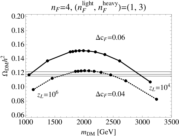
Refer to caption
Figure 8: Relic density of the dark fermion versus mDM=mFlm_{\rm DM}=m_{F_{l}} for nF=4n_{F}=4 (nFlight=1,nFheavy=3n_{F}^{\rm light}=1,n_{F}^{\rm heavy}=3). Thick-solid and thick-dotted lines are Δ​cF≡cFl−cFh=0.06\Delta c_{F}\equiv c_{F_{l}}-c_{F_{h}}=0.06 and 0.040.04, respectively. Data points are, from right to left, zL=104z_{L}=10^{4} to 10510^{5} with an interval 10410^{4}, 3×1053\times 10^{5} and 10610^{6}. Horizontal lines around ΩDM​h2∼0.12\Omega_{\rm DM}h^{2}\sim 0.12 show the observed 68% confidence level (CL) limit of the relic density of the cold dark matter.

In Fig. 8 we have plotted the relic density of the dark fermion determined from the Boltzmann equation (3.54) for Δ​cF=0.04\Delta c_{F}=0.04 and 0.060.06 in the case of nF=4n_{F}=4 with (nFlight,nFheavy)=(1,3)(n_{F}^{\rm light},n_{F}^{\rm heavy})=(1,3). For Δ​cF<0.04\Delta c_{F}<0.04, the approximated formula (3.54) is no more valid, and the relic-density can be much larger than those for Δ​cF≳0.04\Delta c_{F}\gtrsim 0.04. By inter-/extra-polating the ΩDM​h2\Omega_{\rm DM}h^{2} with respect to Δ​cF\Delta c_{F} and zLz_{L}, we plot the parameter region (Δ​cF,zL)(\Delta c_{F},z_{L}) allowed by the experimental limit on the current relic density in Fig. 9.

Figure 9: Parameter region (Δ​cF,zL)(\Delta c_{F},z_{L}) allowed by the limits of relic density. Inner and outer colored regions are allowed with the 68% CL limit and twice of the 68% CL limit ΩDM​h2⊂[0.1186±2×0.0031]\Omega_{\rm DM}h^{2}\subset[0.1186\pm 2\times 0.0031], respectively. Mass of the dark fermion mFlm_{F_{l}} and a mass ratio η≡(mFh−mFl)/mFl\eta\equiv(m_{F_{h}}-m_{F_{l}})/m_{F_{l}} are also indicated as solid and dashed lines, respectively.

It is seen that the observed current relic density is obtained when 104≲zL≲10610^{4}\lesssim z_{L}\lesssim 10^{6} (0.07≲θH≲0.170.07\lesssim\theta_{H}\lesssim 0.17) in the range 0.04≲Δ​cF≲0.070.04\lesssim\Delta c_{F}\lesssim 0.07. The mass of the dark fermion mD​Mm_{DM} varies within the range of [1000, 3100]​GeV[1000,\,3100]\,\text{GeV}. For nF=5,6n_{F}=5,6 and nF=4n_{F}=4 with (nFlight,nFheavy)=(2,2)(n_{F}^{\rm light},n_{F}^{\rm heavy})=(2,2), (3,1)(3,1), we find no parameter region which explains the current DM density.

In the numerical study we have used an approximation explained in Sec. 3.2. In the case where the Breit-Wigner resonance enhance the DM relic density, a more rigorous treatment may be required.[71] In the case under consideration, the effect of the enhancement is found to be mild. Quantitatively, in the notation of Ref. [71] we obtain ϵ=(ΓV/mV)2=𝒪⁡(0.005)\epsilon=(\Gamma_{V}/m_{V})^{2}={\cal O}(0.005) (V=Z(1),ZR(1),γ(1)V=Z^{(1)},Z_{R}^{(1)},\gamma^{(1)}) and u=2​mF/mV≲0.8\sqrt{u}=2m_{F}/m_{V}\lesssim 0.8. In this parameter region the approximation can be justified.[71]

Before closing this section, we make a few comments. First we comment on the effect of dark fermions on the electroweak precision parameters [77], in particular on the SS-parameter. Since the dark fermions have vector-like couplings to the ZZ boson, the contribution to the SS parameter from an S​U​(2)SU(2) doublet {F+,F0}\{F^{+},F^{0}\} is estimated to be

Δ⁡(αEM​S)\displaystyle\Delta(\alpha_{\rm EM}S) ≃\displaystyle\simeq 4​sw2​cw2​Π′​(0)​∑F=F+,F0((gF​VZ)2−cw2−sw2cw​sw​gF​VZ​QF​e−QF2​e2),\displaystyle 4s_{w}^{2}c_{w}^{2}\Pi^{\prime}(0)\sum_{F=F^{+},F^{0}}\left((g^{Z}_{FV})^{2}-\frac{c_{w}^{2}-s_{w}^{2}}{c_{w}s_{w}}g^{Z}_{FV}Q_{F}e-Q_{F}^{2}e^{2}\right), (3.55)
cw≡cos⁡θW,sw≡sin⁡θW,\displaystyle c_{w}\equiv\cos\theta_{W},\quad s_{w}\equiv\sin\theta_{W},

where gF​VZ≡(gF​LZ+gF​RZ)/2g^{Z}_{FV}\equiv(g^{Z}_{FL}+g^{Z}_{FR})/2 and QFQ_{F} is the vector coupling to ZZ and the electric charge of FF, respectively. Π⁡(p2)\Pi(p^{2}) is the vacuum polarization function which is induced by the one-loop fermion with vector-type coupling. Numerically we find that in both cases of FlF_{l} (ηFl=+1\eta_{F_{l}}=+1) and FhF_{h} (ηFh=−1\eta_{F_{h}}=-1) the sum of the right-hand side in (3.55) vanishes accurately. Hence there are no sizable corrections of the SS parameter from dark fermions.

Secondly as an stabilization mechanism of the branes one can introduce some dynamical model a la Goldberger-Wise[78]. In such a case the phase transition of the radion field may alter the thermal history of the universe drastically[79]. Here we have supposed that the critical temperature of the radion phase transition, TϕT_{\phi}, is much higher than the freeze-out temperature of the dark fermions, e.g., Tϕ≫Tf∼100​GeVT_{\phi}\gg T_{f}\sim 100\,\text{GeV}.

4 Direct detection

In this section, we analyse the elastic scattering of the dark fermion (F0F^{0}) off a nucleus [35, 36, 80] and examine the constraint coming from direct detection experiments.[63, 64] The dominant process of the F0F^{0}-nucleus scattering turns out the ZZ boson exchange, though the ZZ-F0F^{0} coupling is very small. The ZR(n)Z_{R}^{(n)}-F0F^{0} coupling is larger, but ZR(n)Z_{R}^{(n)} is heavy. Subdominant are the processes of ZR(1)Z_{R}^{(1)} and Higgs exchange. Contributions from other processes are negligible.

Refer to caption Refer to caption Refer to caption
Figure 10: Dominant and subdominant processes of the F0F^{0}-nucleus scattering

In the scattering of F0F^{0} on nuclei with large mass number AA, scalar and vector interactions dominate for the spin-independent cross section. Therefore the effective Lagrangian at low energies is given by

ℒint≃∑q{−(gw2​vqmZ2cosθW2​VF+gw2​vq(ZR(1))mZR(1)2​VF(ZR(1)))​q¯​γ0​q​F0¯​γ0​F0+yq​YFmH2​q¯​q​F0¯​F0}.\mathcal{L}_{\text{int}}\simeq\sum_{q}\Bigg\{-\bigg(\frac{g_{w}^{2}v_{q}}{m_{Z}^{2}\cos\theta_{W}^{2}}V_{F}+\frac{g_{w}^{2}v^{(Z_{R}^{(1)})}_{q}}{m_{Z_{R}^{(1)}}^{2}}V^{(Z_{R}^{(1)})}_{F}\bigg)\bar{q}\gamma^{0}q\;\bar{F^{0}}\gamma_{0}F^{0}+\frac{y_{q}Y_{F}}{m_{H}^{2}}\bar{q}q\bar{F^{0}}F^{0}\Bigg\}. (4.1)

To evaluate the scattering amplitude by the Higgs exchange, we need estimate the nucleon matrix element

⟨N|mq​q¯​q|N⟩=mN​fT​q(N),\langle N|m_{q}\bar{q}q|N\rangle=m_{N}f^{(N)}_{Tq}, (4.2)

where N=p,nN=p,n. For heavy quarks (Q=cQ=c, bb, tt) one has

fT​Q(N)=227​(1−∑q=u,d,sfT​q(N)).f^{(N)}_{TQ}=\frac{2}{27}\bigg(1-\sum_{q=u,d,s}f^{(N)}_{Tq}\bigg). (4.3)

In the GHU model, quark couplings satisfy vq|GHU≃vq|SMv_{q}|_{\text{GHU}}\simeq v_{q}|_{\text{SM}} and

yq|GHU≃yq|SMcosθH=gw2​mWmqcosθH,y_{q}|_{\text{GHU}}\simeq y_{q}|_{\text{SM}}\cos\theta_{H}=\frac{g_{w}}{2m_{W}}m_{q}\cos\theta_{H}, (4.4)

to good accuracy.[21] Therefore, by dropping the small momentum dependence of the form factor, the spin-independent cross section of the F0F^{0}-nucleus elastic scattering becomes

σ0\displaystyle\sigma_{0} ≡∫04​Mr2​v2d​σd​|𝒒|2||𝒒|=0​d​|𝒒|2\displaystyle\equiv\int_{0}^{4M_{r}^{2}v^{2}}\frac{d\sigma}{d|\bm{q}|^{2}}\bigg|_{|\bm{q}|=0}d|\bm{q}|^{2}
=Mr2π​{Z⁡(bp+fp)+(A−Z)​(bn+fn)}2,\displaystyle=\frac{M_{r}^{2}}{\pi}\Big\{Z\left(b_{p}+f_{p}\right)+(A-Z)\left(b_{n}+f_{n}\right)\Big\}^{2}, (4.5)

where MrM_{r} is the F0F^{0}-nucleus reduced mass and ZZ (AA) is the atomic (mass) number of the nucleus. |𝒒||\bm{q}| is the momentum transfer and

bp=2​bu+bd,bn=bu+2​bd,\displaystyle\hskip-28.45274ptb_{p}=2b_{u}+b_{d}~,~~b_{n}=b_{u}+2b_{d}~, (4.6)
bq=−4​2​GF​(vq​VF+mW2mZR(1)2​vq(ZR(1))​VF(ZR(1))),\displaystyle\hskip-28.45274ptb_{q}=-4\sqrt{2}G_{F}\bigg(v_{q}V_{F}+\frac{m_{W}^{2}}{m_{Z_{R}^{(1)}}^{2}}v^{(Z_{R}^{(1)})}_{q}V^{(Z_{R}^{(1)})}_{F}\bigg)~, (4.7)
fN=YFmH2∑q⟨N|yqq¯q|N⟩=YFmH2gw​mN2​mWcosθH(29+79∑q=u,d,sfT​q(N)).\displaystyle\hskip-28.45274ptf_{N}=\frac{Y_{F}}{m_{H}^{2}}\sum_{q}\langle N|y_{q}\bar{q}q|N\rangle=\frac{Y_{F}}{m_{H}^{2}}\frac{g_{w}m_{N}}{2m_{W}}\cos\theta_{H}\bigg(\frac{2}{9}+\frac{7}{9}\sum_{q=u,d,s}f^{(N)}_{Tq}\bigg)~. (4.8)

The spin-independent cross section of the F0F^{0}-nucleon elastic scattering σN\sigma_{N} can be written as

σN≡1A2​mr2Mr2​σ0,\displaystyle\sigma_{N}\equiv\frac{1}{A^{2}}\frac{m_{r}^{2}}{M_{r}^{2}}\sigma_{0}~, (4.9)

where mrm_{r} is the F0F^{0}-nucleon reduced mass.

The F0F^{0}-nucleon cross sections σN\sigma_{N} are shown in Table 4 and Figure 11. In the numerical evaluation we have employed the values given by [36]

fT​u(p)\displaystyle f^{(p)}_{Tu} =0.020,fT​d(p)=0.026,fT​s(p)=0.118,\displaystyle=0.020~,~~f^{(p)}_{Td}=0.026~,~~f^{(p)}_{Ts}=0.118~,
fT​u(n)\displaystyle f^{(n)}_{Tu} =0.014,fT​d(n)=0.036,fT​s(n)=0.118.\displaystyle=0.014~,~~f^{(n)}_{Td}=0.036~,~~f^{(n)}_{Ts}=0.118~. (4.10)

Recent lattice simulations show smaller values for fT​s(N)f^{(N)}_{Ts} [81], which yields slightly smaller cross sections than those described below.

Table 4: F0F^{0} mass mFm_{F} and the spin-independent cross section σN\sigma_{N} of the F0F^{0}-nucleon scattering for nF=4,5,6n_{F}=4,5,6 degenerate dark fermions.
nF=4n_{F}=4
zLz_{L} θH\;\quad\theta_{H}\quad\; mF\;m_{F} (TeV)    σN​(cm2CLOSE\sigma_{N}\;(\text{cm}^{2})
10510^{5} 0.115 2.03 5.33×10−44\times 10^{-44}
5×1045\times 10^{4} 0.101 2.36 3.78×10−44\times 10^{-44}
3×1043\times 10^{4} 0.092 2.66 2.99×10−44\times 10^{-44}
2×1042\times 10^{4} 0.085 2.92 2.53×10−44\times 10^{-44}
10410^{4} 0.074 3.46 2.03×10−44\times 10^{-44}
nF=5n_{F}=5
zL\;\;\;\;z_{L}\;\;\;\; θH\;\quad\theta_{H}\quad\; mF\;m_{F} (TeV) σN​(cm2CLOSE\quad\;\sigma_{N}\;(\text{cm}^{2})
10510^{5} 0.114 1.75 3.67×10−44\times 10^{-44}
10410^{4} 0.073 2.91 1.01×10−44\times 10^{-44}
nF=6n_{F}=6
zL\;\;\;\;z_{L}\;\;\;\; θH\;\quad\theta_{H}\quad\; mF\;m_{F} (TeV) σN​(cm2CLOSE\quad\;\sigma_{N}\;(\text{cm}^{2})
10510^{5} 0.113 1.57 2.96×10−44\times 10^{-44}
10410^{4} 0.072 2.56 0.72×10−44\times 10^{-44}
Table 5: mFlm_{F_{l}}, mZR(1)m_{Z_{R}^{(1)}}, the couplings of Fl0F^{0}_{l} and the spin-independent cross section σN\sigma_{N} of the Fl0F^{0}_{l}-nucleon scattering for nF=4n_{F}=4 and (nFlight,nFheavy)=(1,3)(n_{F}^{\rm light},n_{F}^{\rm heavy})=(1,3). VFV_{F}, vq(ZR(1))v_{q}^{(Z_{R}^{(1)})} (q=u,dq=u,d), YFY_{F} are defined in Eq. (4.1).
Δ​cF=0.04\Delta c_{F}=0.04
zLz_{L} θH\theta_{H} mFlm_{F_{l}} mZR(1)m_{Z_{R}^{(1)}} VFV_{F} vu(ZR(1))v_{u}^{(Z_{R}^{(1)})} vd(ZR(1))v_{d}^{(Z_{R}^{(1)})} VF(ZR(1))V_{F}^{(Z_{R}^{(1)})} YFY_{F} σN\sigma_{N} (cm2\text{cm}^{2})
(TeV) (TeV)
4×1044\times 10^{4} 0.097 2.29 6.47 -0.00108 0.474 -0.237 1.11 -0.0299 2.69×10−44\times 10^{-44}
3×1043\times 10^{4} 0.092 2.46 6.74 -0.00100 0.469 -0.234 1.11 -0.0293 2.35×10−44\times 10^{-44}
2×1042\times 10^{4} 0.085 2.72 7.15 -0.00092 0.461 -0.231 1.10 -0.0286 1.96×10−44\times 10^{-44}
10410^{4} 0.074 3.24 7.92 -0.00081 0.450 -0.225 1.08 -0.0280 1.53×10−44\times 10^{-44}
Δ​cF=0.06\Delta c_{F}=0.06
zLz_{L} θH\theta_{H} mFlm_{F_{l}} mZR(1)m_{Z_{R}^{(1)}} VFV_{F} vu(ZR(1))v_{u}^{(Z_{R}^{(1)})} vd(ZR(1))v_{d}^{(Z_{R}^{(1)})} VF(ZR(1))V_{F}^{(Z_{R}^{(1)})} YFY_{F} σN\sigma_{N} (cm2\text{cm}^{2})
(TeV) (TeV)
2×1042\times 10^{4} 0.085 2.61 7.15 -0.00086 0.461 -0.231 1.09 -0.0266 1.76×10−44\times 10^{-44}
10410^{4} 0.074 3.13 7.92 -0.00075 0.450 -0.225 1.07 -0.0261 1.35×10−44\times 10^{-44}
Figure 11: The spin-independent cross section of the F0F^{0}-nucleon elastic scattering for 104≤zL≤10510^{4}\leq z_{L}\leq 10^{5}. The orange diamonds and light blue stars represent the nF=4n_{F}=4 and nF=5n_{F}=5 cases of degenerate dark fermions with a step of 10410^{4} in zLz_{L}, respectively. Red circles and blue squares represent the cases of non-degenerate dark fermions (nFlight,nFheavy)=(1,3)(n_{F}^{\rm light},n_{F}^{\rm heavy})=(1,3) with Δ​cF=0.04\Delta c_{F}=0.04 and 0.06, respectively. The black solid line and green dashed line are the 90% confidence limits set by the 85.3 live-days result of the LUX experiment[64] and the 225 live-days result of the XENON100 experiment[63], respectively. For reference we have added the expected limit by the 300 live-days result of the LUX experiment. The XENON 1T experiment is expected to give a limit one order of magnitude smaller than that of the LUX 300 live-days experiment in the cross-section. The purple and light purple bands represent the regions allowed by the limit of the relic density of DM at the 68 % CL depicted in Fig.  9 and by twice of that. The model with dark fermions of 2.3​TeV<mFl<3.12.3\,{\rm TeV}<m_{F_{l}}<3.1\,TeV (4×10⁴>zL>1044\times 10^{4}>z_{L}>10^{4}) gives a consistent scenario.

In the previous section we have seen that when all nFn_{F} dark fermions are degenerate, there are no parameter regions which reproduce the observed value of the relic DM density. It was shown that the observed DM density can be obtained when there are nFlightn_{F}^{\rm light} light dark fermions and nFheavyn_{F}^{\rm heavy} heavy dark fermions of opposite ηF\eta_{F} in the boundary conditions. In particular, for the parameter set of (nFlight,nFheavy)=(1,3)(n_{F}^{\rm light},n_{F}^{\rm heavy})=(1,3), the region 0.04​<∼​Δ​cF​<∼​0.070.04\hskip 3.00003pt\raisebox{1.72218pt}{$<$}\hskip-7.5pt\raisebox{-3.01385pt}{$\sim$}\hskip 3.00003pt\Delta c_{F}\hskip 3.00003pt\raisebox{1.72218pt}{$<$}\hskip-7.5pt\raisebox{-3.01385pt}{$\sim$}\hskip 3.00003pt0.07, zL​<∼​106z_{L}\hskip 3.00003pt\raisebox{1.72218pt}{$<$}\hskip-7.5pt\raisebox{-3.01385pt}{$\sim$}\hskip 3.00003pt10^{6} successfully explains the relic abundance as shown in Fig. 9. The allowed band region in Fig. 9 is mapped in Fig. 11 for the spin-independent cross section for the F0F^{0}-nucleon elastic scattering. The purple and light purple bands there represent the regions allowed by the limit of the relic abundance of DM at the 68 % CL and by twice of that, respectively. It is seen that the band region from zL=104z_{L}=10^{4} to 4×1044\times 10^{4} is allowed by the direct detection experiments of LUX [64] and XENON100 [63]. In the allowed region the dark fermion mass ranges from 3.1 TeV to 2.3 TeV, whereas the AB phase θH\theta_{H} ranges from 0.074 to 0.097. The mass of Z′Z^{\prime} bosons (the lowest ZRZ_{R} boson and the first KK modes Z(1)Z^{(1)} and γ(1)\gamma^{(1)}) ranges from 8 TeV to 6.5 TeV. For reference we have added, in Fig. 11, the expected limit by the 300 live-days result of the LUX experiment. The XENON 1T experiment is expected to give a limit one order of magnitude smaller than that of the LUX 300 live-days experiment in the cross-section.

We remark that the nF=3n_{F}=3 case predicts too small relic densities as shown in Fig. 8. It implies that the dark fermions in the GHU model accounts for only a fraction of the dark matter of the universe, and the model is not excluded by the direct-detection experiments.

5 Conclusion and discussions

In the present paper we have given a detailed analysis of DM in GHU. In the S​O​(5)×U⁡(1)SO(5)\times U(1) GHU, the observed unstable Higg boson is realized by introducing S​O​(5)SO(5)-spinor fermions. Spinor fermions do not directly interact with S​O​(5)SO(5)-vector fermions which contain the SM quarks and leptons. Therefore the total spinor-fermion number is conserved and the lightest one can remain as dark matter in the current universe. Such fermions are referred to as “dark fermions”.

In Sec. 3 we have evaluated the relic density of the dark fermions. Although charged and neutral dark fermions are degenerate at tree level, charged fermions become heavier than neutral ones through loop effects so that the charged dark fermions decay into neutral ones much earlier than they cooled down at their freeze-out temperature. We found that among various annihilation processes of dark fermions dominant ones are those in which a dark fermion and its antiparticle annihilate into the SM fermions mediated by the lowest KK ZRZ_{R} boson and the first KK photon. We also have evaluated the annihilation cross section and obtained the relic densities of the dark fermions in the current universe for the various values of nFn_{F} and zLz_{L}. The results depend sensitively on the number of dark fermions nFn_{F}. When all neutral dark fermions are degenerate, no solution has been found which explains the observed value of the relic density of dark matter and is consistent with the limit from the direct detection experiments. For nF=3n_{F}=3 the relic density becomes much smaller than the bound, because twice the mass of the dark fermion is close to the mass of the ZRZ_{R} boson and the annihilation is enhanced by the resonance. For nF=4,5n_{F}=4,5 and 66 the relic densitiy becomes larger than the bound.

We have considered the case in which nFn_{F} dark fermions consist of nFlightn_{F}^{\rm light} lighter fermions and nFheavyn_{F}^{\rm heavy} heavier fermions. They are mixed with each other through the bulk mass terms which can be introduced when lighter and heavier fermions have opposite signs of ηF\eta_{F} in the boundary conditions under reflections at the TeV and Planck branes. When the mass difference of these fermions are sufficiently large (more than 𝒪⁡(100​GeV){\cal O}(100\text{GeV})), heavier ones decay quickly to lighter ones and the effective number of species of the dark fermions can be reduced from nFn_{F} to nFlightn_{F}^{\rm light}. Accordingly the relic density reduces to nFlight/nFn_{F}^{\rm light}/n_{F} of that in the degenerate case. For nF=4n_{F}=4 it is found that one can obtain the relic density consistent with the experimental bound for 104≲zL≲10610^{4}\lesssim z_{L}\lesssim 10^{6} , 0.04≲Δ​cF≲0.070.04\lesssim\Delta c_{F}\lesssim 0.07 when (nFlight,nFheavy)=(1,3)(n_{F}^{\rm light},n_{F}^{\rm heavy})=(1,3). In the cases of (nFlight,nFheavy)=(2,2),(3,1)(n_{F}^{\rm light},n_{F}^{\rm heavy})=(2,2),(3,1) and of nF=5n_{F}=5 and =6=6 no solution has been found. We comment that there are no sizable corrections to the SS-parameter from the dark-fermion loops.

In Sec. 4, we calculated the scattering cross section of the dark fermions with nucleons. The dark fermions have very small Higgs-Yukawa couplings and ZZ-boson couplings, both of which are suppressed by powers of sin⁡θH\sin\theta_{H}. We evaluated the spin-independent cross sections and compared with the experimental bound obtained in the recent experiments of WIMP direct detection.[63, 64] Combining with the constraint from the relic density, we showed that the region 104≲zL≲4×10410^{4}\lesssim z_{L}\lesssim 4\times 10^{4} for (nFlight,nFheavy)=(1,3)(n_{F}^{\rm light},n_{F}^{\rm heavy})=(1,3) is viable. The corresponding mass of the dark matter candidate (dark fermions) ranges from 3.1 TeV to 2.3 TeV, whereas the AB phase θH\theta_{H} ranges from 0.074 to 0.097. The mass of Z′Z^{\prime} bosons ranges from 8 TeV to 6.5 TeV.

The nF=4n_{F}=4 model with one light and three heavy dark fermions with opposite boundary conditions is consistent with the current direct detection experiments. Such dark fermions should be detected in the direct-detection experiments in near future. For nF=3n_{F}=3, our model cannot explain the current DM density. In this case the current DM density should be accounted for by dark matter generated by other mechanism such as axion DM [51] and dynamical dark matter [58]. In this case DM in the GHU model may or may not be detected, depending on the property of the dominant dark matter components.

The gauge-Higgs unification scenario is viable and promising. The S​O​(5)×U⁡(1)SO(5)\times U(1) GHU predicts new Z′Z^{\prime} bosons in the 6.5 TeV∼\sim8 TeV region and deviation of the self-couplings of the Higgs boson from SM, which can be explored and checked at the upgraded LHC and ILC experiments. We stress again that the model naturally contains the dark matter candidate (dark fermions) in the mass range 2.3 TeV∼\sim3.1 TeV. The mass and cross section of the dark fermions are within the reach of the ongoing and future experiments, and the allowed parameter region of this model can be explored with future collider experiments [16]. Pinning down its mass fixes the value of θH\theta_{H}, which further yields more predictions of GHU in collider experiments.

Acknowledgements

We thank Mitsuru Kakizaki and Minoru Tanaka for many valuable comments. This work was supported in part by JSPS KAKENHI grants, No. 23104009 (YH and YO), No. 21244036 (YH) and No. 2518610 (TS), and NRF Research Grant 2012R1A2A1A01006053 (HH), No. 2009-0083526 (YO) of the Republic of Korea.

Appendix A S​O​(5)SO(5) generators and base functions

S​O​(5)SO(5) generators in the spinorial representation are defined as

TLa=12​(σa),TRa=12​(σa),\displaystyle T_{L}^{a}=\frac{1}{2}\begin{pmatrix}\sigma^{a}&\\ &\end{pmatrix},\quad T_{R}^{a}=\frac{1}{2}\begin{pmatrix}&\\ &\sigma^{a}\end{pmatrix}, (A.1)
T^a=12​2​(i​σa−i​σa),T^4=12​2​(II),\displaystyle\hat{T}^{a}=\frac{1}{2\sqrt{2}}\begin{pmatrix}&i\sigma^{a}\\ -i\sigma^{a}&\end{pmatrix},\quad\hat{T}^{4}=\frac{1}{2\sqrt{2}}\begin{pmatrix}&I\\ I&\end{pmatrix}, (A.2)

and Tr⁡[Tα,Tβ]=δα​β{\rm Tr\,}[T^{\alpha},T^{\beta}]=\delta^{\alpha\beta} holds.

Mode functions for KK towers are expressed in terms of Bessel functions. For gauge fields we define

C⁡(z,λ)=π2​λ​z​zL​F1,0​(λ​z,λ​zL),C′​(z,λ)=π2​λ2​z​zL​F0,0​(λ​z,λ​zL),\displaystyle\hskip-28.45274ptC(z;\lambda)=\frac{\pi}{2}\lambda zz_{L}F_{1,0}(\lambda z,\lambda z_{L})~,\quad C^{\prime}(z;\lambda)=\frac{\pi}{2}\lambda^{2}zz_{L}F_{0,0}(\lambda z,\lambda z_{L})~, (A.3)
S⁡(z,λ)=−π2​λ​z​F1,1​(λ​z,λ​zL),S′​(z,λ)=−π2​λ2​z​F0,1​(λ​z,λ​zL),\displaystyle\hskip-28.45274ptS(z;\lambda)=-\frac{\pi}{2}\lambda zF_{1,1}(\lambda z,\lambda z_{L})~,\quad S^{\prime}(z;\lambda)=-\frac{\pi}{2}\lambda^{2}zF_{0,1}(\lambda z,\lambda z_{L})~, (A.4)
S^​(z,λ)=C⁡(1,λ)S⁡(1,λ)​S​(z,λ),\displaystyle\hskip-28.45274pt\hat{S}(z;\lambda)=\frac{C(1;\lambda)}{S(1;\lambda)}\,S(z;\lambda)~, (A.5)
Fα,β​(u,v)=Jα​(u)​Yβ​(v)−Yα​(u)​Jβ​(v).\displaystyle\hskip-28.45274ptF_{\alpha,\beta}(u,v)=J_{\alpha}(u)Y_{\beta}(v)-Y_{\alpha}(u)J_{\beta}(v)~. (A.6)

These functions satisfy

C⁡(zL,λ)=zL,C′​(zL,λ)=0,S⁡(zL,λ)=0,S′​(zL,λ)=λ,\displaystyle\hskip-28.45274ptC(z_{L};\lambda)=z_{L}~,~~C^{\prime}(z_{L};\lambda)=0~,~~S(z_{L};\lambda)=0~,~~S^{\prime}(z_{L};\lambda)=\lambda~, (A.7)
C​S′−S​C′=λ​z.\displaystyle\hskip-28.45274ptCS^{\prime}-SC^{\prime}=\lambda z~. (A.8)

For fermions with a bulk mass parameter cc we define

(CLSL)⁡(z,λ,c)=±π2​λ​z​zL​Fc+12,c∓12​(λ​z,λ​zL),\displaystyle\hskip-28.45274pt\begin{pmatrix}C_{L}\cr S_{L}\end{pmatrix}(z;\lambda,c)=\pm\frac{\pi}{2}\lambda\sqrt{zz_{L}}F_{c+{1\over 2},c\mp{1\over 2}}(\lambda z,\lambda z_{L})~, (A.9)
(CRSR)⁡(z,λ,c)=∓π2​λ​z​zL​Fc−12,c±12​(λ​z,λ​zL).\displaystyle\hskip-28.45274pt\begin{pmatrix}C_{R}\cr S_{R}\end{pmatrix}(z;\lambda,c)=\mp\frac{\pi}{2}\lambda\sqrt{zz_{L}}F_{c-{1\over 2},c\pm{1\over 2}}(\lambda z,\lambda z_{L})~. (A.10)

They satisfy

D+​(c)​(CLSL)=λ​(SRCR),D−​(c)​(CRSR)=λ​(SLCL),D±​(c)=±dd​z+cz,D_{+}(c)\begin{pmatrix}C_{L}\cr S_{L}\end{pmatrix}=\lambda\begin{pmatrix}S_{R}\cr C_{R}\end{pmatrix}~~,~~D_{-}(c)\begin{pmatrix}C_{R}\cr S_{R}\end{pmatrix}=\lambda\begin{pmatrix}S_{L}\cr C_{L}\end{pmatrix}~~,~~D_{\pm}(c)=\pm\frac{d}{dz}+\frac{c}{z}~~, (A.11)

and

CR=CL=1,SR=SL=0,at​z=zL,\displaystyle\hskip-28.45274ptC_{R}=C_{L}=1~,~~S_{R}=S_{L}=0~,~~{\rm at~}z=z_{L}~, (A.12)
CL​CR−SL​SR=1.\displaystyle\hskip-28.45274ptC_{L}C_{R}-S_{L}S_{R}=1~. (A.13)

Appendix B Wave functions of dark fermions

The dark fermion ΨFi\Psi_{F_{i}} is introduced in the spinorial representation of S​O​(5)SO(5). With the charge assignment of QE=T3L+T3R+QXQ_{E}=T^{3_{L}}+T^{3_{R}}+Q_{X} and QX=12Q_{X}=\hbox{$\frac{1}{2}$}, ΨFi​(x,z)\Psi_{F_{i}}(x,z) is decomposed into KK modes Fi+(n)​(x)F_{i}^{+(n)}(x) and Fi0​(n)​(x)F_{i}^{0(n)}(x) (n=1,2,3,⋯n=1,2,3,\cdots) in the twisted gauge in which ⟨​Az​⟩\raise 0.68889pt\hbox{$\langle$}\lower 0.68889pt\hbox{}A_{z}\raise 0.68889pt\hbox{$\rangle$}\lower 0.68889pt\hbox{} vanishes.

ΨFi=ΨFi,R+ΨFi,L=∑nΨFi(n),ΨFi(n)=ΨFi,R(n)+ΨFi,L(n),\displaystyle\hskip-28.45274pt\Psi_{F_{i}}=\Psi_{F_{i},R}+\Psi_{F_{i},L}=\sum_{n}\Psi_{F_{i}}^{(n)}~~,~~\Psi_{F_{i}}^{(n)}=\Psi_{F_{i},R}^{(n)}+\Psi_{F_{i},L}^{(n)}~~, (B.1)
γ5​(ΨFi,RΨFi,L)=(+ΨFi,R−ΨFi,L),\displaystyle\hskip-28.45274pt\gamma^{5}\begin{pmatrix}\Psi_{F_{i},R}\cr\Psi_{F_{i},L}\end{pmatrix}=\begin{pmatrix}+\Psi_{F_{i},R}\cr-\Psi_{F_{i},L}\end{pmatrix}~, (B.2)
ΨFi,R(n)​(x,z)=k​z2​{(fi,l​R(n)​(z)0fi,r​R(n)​(z)0)​Fi,R+(n)​(x)+(0fi,l​R(n)​(z)0fi,r​R(n)​(z))​Fi,R0​(n)​(x)},\displaystyle\hskip-28.45274pt\Psi_{F_{i},R}^{(n)}(x,z)=\sqrt{k}z^{2}\left\{\begin{pmatrix}f_{i,lR}^{(n)}(z)\cr 0\cr f_{i,rR}^{(n)}(z)\cr 0\end{pmatrix}F^{+(n)}_{i,R}(x)+\begin{pmatrix}0\cr f_{i,lR}^{(n)}(z)\cr 0\cr f_{i,rR}^{(n)}(z)\end{pmatrix}F^{0(n)}_{i,R}(x)\right\}, (B.3)
ΨFi,L(n)​(x,z)=k​z2​{(fi,l​L(n)​(z)0fi,r​L(n)​(z)0)​Fi,L+(n)​(x)+(0fi,l​L(n)​(z)0fi,r​L(n)​(z))​Fi,L0​(n)​(x)}.\displaystyle\hskip-28.45274pt\Psi_{F_{i},L}^{(n)}(x,z)=\sqrt{k}z^{2}\left\{\begin{pmatrix}f_{i,lL}^{(n)}(z)\cr 0\cr f_{i,rL}^{(n)}(z)\cr 0\end{pmatrix}F^{+(n)}_{i,L}(x)+\begin{pmatrix}0\cr f_{i,lL}^{(n)}(z)\cr 0\cr f_{i,rL}^{(n)}(z)\end{pmatrix}F^{0(n)}_{i,L}(x)\right\}. (B.4)

Here the suffixes ll and rr refer to two S​U​(2)SU(2)’s of S​O​(4)=S​U​(2)L×S​U​(2)R⊂S​O​(5)SO(4)=SU(2)_{L}\times SU(2)_{R}\subset SO(5).

ΨFi\Psi_{F_{i}} in the twisted gauge satisfies a free Dirac equation. The left- and right-handed components of Ψ~Fi=z−2​ΨFi\tilde{\Psi}_{F_{i}}=z^{-2}\Psi_{F_{i}} satisfy

σ⋅∂Ψ~Fi,L=k​D−​(c)​Ψ~Fi,R,\displaystyle\hskip-28.45274pt\sigma\cdot\partial\,\tilde{\Psi}_{F_{i},L}=kD_{-}(c)\tilde{\Psi}_{F_{i},R}~, (B.5)
σ¯⋅∂Ψ~Fi,R=k​D+​(c)​Ψ~Fi,L.\displaystyle\hskip-28.45274pt\bar{\sigma}\cdot\partial\,\tilde{\Psi}_{F_{i},R}=kD_{+}(c)\tilde{\Psi}_{F_{i},L}~. (B.6)

Let us denote the S​U​(2)LSU(2)_{L} (S​U​(2)RSU(2)_{R}) component of ΨFi,L\Psi_{F_{i},L} by ΨFi,l​L\Psi_{F_{i},lL} (ΨFi,r​L\Psi_{F_{i},rL}), etc. The boundary condition for ΨFi\Psi_{F_{i}} with ηFi=+1\eta_{F_{i}}=+1 in (2.13) is transformed in the twisted gauge in the coformal coordinates to

cos⁡12​θH​Ψ~Fi,l​L​(1)−i​sin⁡12​θH​Ψ~Fi,r​L​(1)=0,\displaystyle\hskip-28.45274pt\cos\hbox{$\frac{1}{2}$}\theta_{H}\tilde{\Psi}_{F_{i},lL}(1)-i\sin\hbox{$\frac{1}{2}$}\theta_{H}\tilde{\Psi}_{F_{i},rL}(1)=0~, (B.7)
−i​sin⁡12​θH​Ψ~Fi,l​R​(1)+cos⁡12​θH​Ψ~Fi,r​R​(1)=0,\displaystyle\hskip-28.45274pt-i\sin\hbox{$\frac{1}{2}$}\theta_{H}\tilde{\Psi}_{F_{i},lR}(1)+\cos\hbox{$\frac{1}{2}$}\theta_{H}\tilde{\Psi}_{F_{i},rR}(1)=0~, (B.8)
cos⁡12​θH​D−​Ψ~Fi,l​R​(1)−i​sin⁡12​θH​D−​Ψ~Fi,r​R​(1)=0,\displaystyle\hskip-28.45274pt\cos\hbox{$\frac{1}{2}$}\theta_{H}\,D_{-}\tilde{\Psi}_{F_{i},lR}(1)-i\sin\hbox{$\frac{1}{2}$}\theta_{H}\,D_{-}\tilde{\Psi}_{F_{i},rR}(1)=0~, (B.9)
−i​sin⁡12​θH​D+​Ψ~Fi,l​L​(1)+cos⁡12​θH​D+​Ψ~Fi,r​L​(1)=0,\displaystyle\hskip-28.45274pt-i\sin\hbox{$\frac{1}{2}$}\theta_{H}\,D_{+}\tilde{\Psi}_{F_{i},lL}(1)+\cos\hbox{$\frac{1}{2}$}\theta_{H}\,D_{+}\tilde{\Psi}_{F_{i},rL}(1)=0~, (B.10)
Ψ~Fi,l​R​(zL)=0,D+​Ψ~Fi,l​L​(zL)=0,\displaystyle\hskip-28.45274pt\tilde{\Psi}_{F_{i},lR}(z_{L})=0~,~~D_{+}\tilde{\Psi}_{F_{i},lL}(z_{L})=0~, (B.11)
D−​Ψ~Fi,r​R​(zL)=0,Ψ~Fi,r​L​(zL)=0,\displaystyle\hskip-28.45274ptD_{-}\tilde{\Psi}_{F_{i},rR}(z_{L})=0~,~~\tilde{\Psi}_{F_{i},rL}(z_{L})=0~, (B.12)

By making use of (B.12), eigenmodes can be written as

(Ψ~Fi,l​L​(z)Ψ~Fi,r​L​(z))=(A1​CL​(z,λ,cFi)B1​SL​(z,λ,cFi)),\displaystyle\hskip-28.45274pt\begin{pmatrix}\tilde{\Psi}_{F_{i},lL}(z)\cr\tilde{\Psi}_{F_{i},rL}(z)\end{pmatrix}=\begin{pmatrix}A_{1}C_{L}(z;\lambda,c_{F_{i}})\cr B_{1}S_{L}(z;\lambda,c_{F_{i}})\end{pmatrix}, (B.13)
(Ψ~Fi,l​R​(z)Ψ~Fi,r​R​(z))=(A2​SR​(z,λ,cFi)B2​CR​(z,λ,cFi)).\displaystyle\hskip-28.45274pt\begin{pmatrix}\tilde{\Psi}_{F_{i},lR}(z)\cr\tilde{\Psi}_{F_{i},rR}(z)\end{pmatrix}=\begin{pmatrix}A_{2}S_{R}(z;\lambda,c_{F_{i}})\cr B_{2}C_{R}(z;\lambda,c_{F_{i}})\end{pmatrix}. (B.14)

Then (B.10) leads to

M​(A1B1)=M​(A2B2)=0,\displaystyle\hskip-28.45274ptM\begin{pmatrix}A_{1}\cr B_{1}\end{pmatrix}=M\begin{pmatrix}A_{2}\cr B_{2}\end{pmatrix}=0~, (B.15)
M=(cos⁡12​θH​CL​(1)−i​sin⁡12​θH​SL​(1)−i​sin⁡12​θH​SR​(1)cos⁡12​θH​CR​(1)),\displaystyle\hskip-28.45274ptM=\begin{pmatrix}\cos\hbox{$\frac{1}{2}$}\theta_{H}C_{L}(1)&-i\sin\hbox{$\frac{1}{2}$}\theta_{H}S_{L}(1)\cr-i\sin\hbox{$\frac{1}{2}$}\theta_{H}S_{R}(1)&\cos\hbox{$\frac{1}{2}$}\theta_{H}C_{R}(1)\end{pmatrix}, (B.16)

where CL​(z)=CL​(z,λ,cFi),SR​(z)=SR​(z,λ,cFi)C_{L}(z)=C_{L}(z;\lambda,c_{F_{i}}),~S_{R}(z)=S_{R}(z;\lambda,c_{F_{i}}) etc.

The mass spectrum {mFi,n=kλi,n}\{m_{F_{i},n}=k\lambda_{i,n}\} is determined by detM=0\det M=0, or by

CL​(1,λi,n,cFi)​CR​(1,λi,n,cFi)−sin2⁡θH2=0.C_{L}(1;\lambda_{i,n},c_{F_{i}})C_{R}(1;\lambda_{i,n},c_{F_{i}})-\sin^{2}\frac{\theta_{H}}{2}=0~. (B.17)

The corresponding wave functions are given by

(fi,l​L(n)​(z)fi,l​R(n)​(z))=i​sin⁡12​θH​SL​(1)ri(n)​(CL​(z)SR​(z))=cos⁡12​θH​CR​(1)ri′(n)​(CL​(z)SR​(z)),\displaystyle\hskip-28.45274pt\begin{pmatrix}f_{i,lL}^{(n)}(z)\\ f_{i,lR}^{(n)}(z)\end{pmatrix}=\frac{i\sin\hbox{$\frac{1}{2}$}\theta_{H}S_{L}(1)}{\sqrt{r_{i}^{(n)}}}\,\begin{pmatrix}C_{L}(z)\\ S_{R}(z)\end{pmatrix}=\frac{\cos\hbox{$\frac{1}{2}$}\theta_{H}C_{R}(1)}{\sqrt{r_{i}^{\prime(n)}}}\,\begin{pmatrix}C_{L}(z)\\ S_{R}(z)\end{pmatrix}, (B.18)
(fi,r​L(n)​(z)fi,r​R(n)​(z))=cos⁡12​θH​CL​(1)ri(n)​(SL​(z)CR​(z))=i​sin⁡12​θH​SR​(1)ri′(n)​(SL​(z)CR​(z)),\displaystyle\hskip-28.45274pt\begin{pmatrix}f_{i,rL}^{(n)}(z)\\ f_{i,rR}^{(n)}(z)\end{pmatrix}=\frac{\cos\hbox{$\frac{1}{2}$}\theta_{H}C_{L}(1)}{\sqrt{r_{i}^{(n)}}}\,\begin{pmatrix}S_{L}(z)\\ C_{R}(z)\end{pmatrix}=\frac{i\sin\hbox{$\frac{1}{2}$}\theta_{H}S_{R}(1)}{\sqrt{r_{i}^{\prime(n)}}}\,\begin{pmatrix}S_{L}(z)\\ C_{R}(z)\end{pmatrix}, (B.19)

with λ=λi,n\lambda=\lambda_{i,n}. The normalization factors ri(n)r_{i}^{(n)} and ri′(n)r_{i}^{\prime(n)} are determined by the condition

∫1zLd​z​{|fl​L(n)|2+|fr​L(n)|2}=∫1zLd​z​{|fl​R(n)|2+|fr​R(n)|2}=1\displaystyle\int_{1}^{z_{L}}dz\,\big\{|f_{lL}^{(n)}|^{2}+|f_{rL}^{(n)}|^{2}\big\}=\int_{1}^{z_{L}}dz\,\big\{|f_{lR}^{(n)}|^{2}+|f_{rR}^{(n)}|^{2}\big\}=1 (B.20)

to be

ri(n)=∫1zLd​z​{sin2⁡12​θH​SL​(1)2​CL​(z)2+cos2⁡12​θH​CL​(1)2​SL​(z)2}\displaystyle\hskip-28.45274ptr_{i}^{(n)}=\int_{1}^{z_{L}}dz\,\big\{\sin^{2}\hbox{$\frac{1}{2}$}\theta_{H}S_{L}(1)^{2}C_{L}(z)^{2}+\cos^{2}\hbox{$\frac{1}{2}$}\theta_{H}C_{L}(1)^{2}S_{L}(z)^{2}\big\} (B.21)
=∫1zLd​z​{sin2⁡12​θH​SL​(1)2​SR​(z)2+cos2⁡12​θH​CL​(1)2​CR​(z)2},\displaystyle\hskip-17.07182pt=\int_{1}^{z_{L}}dz\,\big\{\sin^{2}\hbox{$\frac{1}{2}$}\theta_{H}S_{L}(1)^{2}S_{R}(z)^{2}+\cos^{2}\hbox{$\frac{1}{2}$}\theta_{H}C_{L}(1)^{2}C_{R}(z)^{2}\big\}, (B.22)
ri′(n)=∫1zLd​z​{cos2⁡12​θH​CR​(1)2​CL​(z)2+sin2⁡12​θH​SR​(1)2​SL​(z)2}\displaystyle\hskip-28.45274ptr_{i}^{\prime(n)}=\int_{1}^{z_{L}}dz\,\big\{\cos^{2}\hbox{$\frac{1}{2}$}\theta_{H}C_{R}(1)^{2}C_{L}(z)^{2}+\sin^{2}\hbox{$\frac{1}{2}$}\theta_{H}S_{R}(1)^{2}S_{L}(z)^{2}\big\} (B.23)
=∫1zLd​z​{cos2⁡12​θH​CR​(1)2​SR​(z)2+sin2⁡12​θH​SR​(1)2​CR​(z)2}.\displaystyle\hskip-17.07182pt=\int_{1}^{z_{L}}dz\,\big\{\cos^{2}\hbox{$\frac{1}{2}$}\theta_{H}C_{R}(1)^{2}S_{R}(z)^{2}+\sin^{2}\hbox{$\frac{1}{2}$}\theta_{H}S_{R}(1)^{2}C_{R}(z)^{2}\big\}. (B.24)

One comment is in order about the θH→0\theta_{H}\rightarrow 0 limit of the wave functions. For θH=0\theta_{H}=0 the spectrum (B.17) is determined by either CR​(1)=CR​(1,λi,2​n−1,cFi)=0C_{R}(1)=C_{R}(1;\lambda_{i,2n-1},c_{F_{i}})=0 or CL​(1)=CL​(1,λi,2​n,cFi)=0C_{L}(1)=C_{L}(1;\lambda_{i,2n},c_{F_{i}})=0 (n=1,2,3,⋯n=1,2,3,\cdots) where eigenvalues have been ordered as 0<λi,1<λi,2<λi,3<⋯0<\lambda_{i,1}<\lambda_{i,2}<\lambda_{i,3}<\cdots. The case CR​(1)=0C_{R}(1)=0 corresponds to excitations of the S​U​(2)RSU(2)_{R} doublet component, whereas CL​(1)=0C_{L}(1)=0 to excitations of the S​U​(2)LSU(2)_{L} doublet component. For CR​(1)=0C_{R}(1)=0 (CL​(1)=0C_{L}(1)=0), ri′(n)/sin2⁡12​θH≠0r_{i}^{\prime(n)}/\sin^{2}\hbox{$\frac{1}{2}$}\theta_{H}\not=0 ( ri(n)/sin2⁡12​θH≠0r_{i}^{(n)}/\sin^{2}\hbox{$\frac{1}{2}$}\theta_{H}\not=0) at θH=0\theta_{H}=0.

In the boundary condition for ΨFi\Psi_{F_{i}}, one could adopt ηFi=−1\eta_{F_{i}}=-1 in (2.13). In the case of non-degenerate dark fermions the heavy dark fermion multiplet satisfies this flipped boundary condition. In this case the corresponding wave functions and Kaluza-Klein masses are obtained from the above formulas by the replacement

cH↔i​sH,CL↔SL,SR↔CR.\displaystyle c_{H}\leftrightarrow is_{H}~,\quad C_{L}\leftrightarrow S_{L}~,\quad S_{R}\leftrightarrow C_{R}~. (B.25)

The spectrum is determined by the same equation as in (B.17). The lowest mode mostly becomes an S​U​(2)LSU(2)_{L} doublet for small θH\theta_{H}.

Appendix C Gauge and Higgs couplings of dark fermions

C.1 Couplings to the Higgs boson

Couplings to the Higgs boson is read from the gauge interaction

∫1zLd​z​G​e4z​Ψ¯F​(gA​Az+QX​gB​Bz)​i​γ5​ΨF,G​e4z​gA=L​gwk4​z4,\displaystyle\int_{1}^{z_{L}}dz\sqrt{G}{e_{4}}^{z}\bar{\Psi}_{F}(g_{A}A_{z}+Q_{X}g_{B}B_{z})i\gamma_{5}\Psi_{F},\quad\sqrt{G}{e_{4}}^{z}g_{A}=\frac{\sqrt{L}g_{w}}{k^{4}z^{4}}, (C.1)

where

Az​(x,z)\displaystyle A_{z}(x,z) =\displaystyle= H^+∑a=13G^a+∑a=13D^a,\displaystyle\hat{H}+\sum_{a=1}^{3}\hat{G}^{a}+\sum_{a=1}^{3}\hat{D}^{a},
H^\displaystyle\hat{H} =\displaystyle= ∑nH(n)​(x)​uH(n)​T4^,\displaystyle\sum_{n}H^{(n)}(x)u_{H^{(n)}}T^{\hat{4}},
G^a\displaystyle\hat{G}^{a} =\displaystyle= ∑nGa⁡(n)​(x)​{uG(n)​TaL+TaR2},\displaystyle\sum_{n}G^{a(n)}(x)\left\{u_{G^{(n)}}\frac{T^{a_{L}}+T^{a_{R}}}{\sqrt{2}}\right\},
D^a\displaystyle\hat{D}^{a} =\displaystyle= ∑nDa⁡(n)​(x)​{uD(n)−​TaL−TaR2+u^D(n)​Ta^},\displaystyle\sum_{n}D^{a(n)}(x)\left\{u_{D^{(n)}}^{-}\frac{T^{a_{L}}-T^{a_{R}}}{\sqrt{2}}+\hat{u}_{D^{(n)}}T^{\hat{a}}\right\},
Bz​(x,z)\displaystyle B_{z}(x,z) =\displaystyle= ∑nB(n)​(x)​uB(n)​(z),\displaystyle\sum_{n}B^{(n)}(x)u_{B^{(n)}}(z), (C.2)

Ga⁡(n)G^{a(n)}, Da⁡(n)D^{a(n)} and B(n)B^{(n)} are NG-bosons and only the H^\hat{H} is the tower of the physical scalar particles. Hereafter we consider only Higgs couplings. The Higgs wave functions are given by

uH(0)​(z)\displaystyle u_{H^{(0)}}(z) =\displaystyle= 2k⁡(zL2−1)​z,\displaystyle\sqrt{\frac{2}{k(z_{L}^{2}-1)}}\,z, (C.3)

for the zero-mode Higgs boson and

uH(n)​(z)\displaystyle u_{H^{(n)}}(z) =\displaystyle= 1rH(n)​S′​(z,λH(n)),rH(n)=∫1zLk​d​zz​S′​(z,λH(n))2,\displaystyle\frac{1}{\sqrt{r_{H^{(n)}}}}S^{\prime}(z;\lambda_{H^{(n)}}),\quad r_{H^{(n)}}=\int_{1}^{z_{L}}\frac{kdz}{z}S^{\prime}(z;\lambda_{H^{(n)}})^{2}, (C.4)

for KK excitations (n≥1n\geq 1). Here S⁡(1,λH(n))=0S(1;\lambda_{H^{(n)}})=0 is satisfied. The building-block for the H​F¯(n)​F(n)H\bar{F}^{(n)}F^{(n)} Yukawa coupling is given by

Ψ¯Fj(n)​γ5​T4^​ΨFj(n)\displaystyle\bar{\Psi}^{(n)}_{F_{j}}\gamma_{5}T^{\hat{4}}\Psi^{(n)}_{F_{j}} =\displaystyle= i​k​z42​2​1rj(n)​sin⁡θH2​cos⁡θH2​SL​(1)​CL​(1)​[F¯j​L(n)​Fj​R(n)−F¯j​R(n)​Fj​L(n)],\displaystyle i\frac{kz^{4}}{2\sqrt{2}}\frac{1}{r_{j}^{(n)}}\sin\frac{\theta_{H}}{2}\cos\frac{\theta_{H}}{2}S_{L}(1)C_{L}(1)[\bar{F}_{jL}^{(n)}F_{jR}^{(n)}-\bar{F}_{jR}^{(n)}F_{jL}^{(n)}], (C.5)

where CL​(z)​CR​(z)−SL​(z)​SR​(z)=1C_{L}(z)C_{R}(z)-S_{L}(z)S_{R}(z)=1 has been made use of. Hence the Higgs Yukawa coupling in the 4D Lagrangian, ℒ4​D⊃yFi(n)​H(0)​F¯i(n)​Fi(n){\cal L}_{4D}\supset y_{F^{(n)}_{i}}H^{(0)}\bar{F}^{(n)}_{i}F^{(n)}_{i}, is given by

yFi(n)=gw4​1ri(n)​k​L​(zL2−1)​sin⁡θH2​cos⁡θH2​SL​(1,λi,n,cF)​CL​(1,λi,n,cF),\displaystyle y_{F^{(n)}_{i}}=\frac{g_{w}}{4}\frac{1}{r_{i}^{(n)}}\sqrt{kL(z_{L}^{2}-1)}\sin\frac{\theta_{H}}{2}\cos\frac{\theta_{H}}{2}S_{L}(1;\lambda_{i,n},c_{F})C_{L}(1;\lambda_{i,n},c_{F}), (C.6)

In Tables 6 and 7, we have summarized the Higgs Yukawa couplings of FF. In Table 7 the couplings in non-degenerate cases are summarized.

Table 6: The Higgs-Yukawa couplings yFi(1)y_{F_{i}^{(1)}} in (C.6) in the case of degenerate dark fermions with the parameters specified in Table 2.
nFn_{F} zLz_{L} yFi(1)y_{F_{i}^{(1)}}
33 10810^{8} −0.106-0.106
10610^{6} −0.071-0.071
10510^{5} −0.064-0.064
2×1042\times 10^{4} −0.089-0.089
44 10810^{8} −0.082-0.082
10610^{6} −0.049-0.049
10510^{5} −0.038-0.038
3×1043\times 10^{4} −0.034-0.034
10410^{4} −0.033-0.033
66 10810^{8} −0.060-0.060
10610^{6} −0.034-0.034
10510^{5} −0.024-0.024
10410^{4} −0.017-0.017
Table 7: The Higgs-Yukawa couplings yFl(1)y_{F_{l}^{(1)}} of the light dark fermion in (C.6) in the case of non-degenerate (nFlight,nFheavy)=(1,3)(n_{F}^{\rm light},n_{F}^{\rm heavy})=(1,3) dark fermions with the parameters specified in Table 3.
Δ​cF\Delta c_{F} zLz_{L} yFl(1)y_{F_{l}^{(1)}}
0.040.04 10610^{6} −0.042-0.042
10510^{5} −0.033-0.033
3×1043\times 10^{4} −0.029-0.029
10410^{4} −0.028-0.028
0.060.06 10610^{6} −0.038-0.038
10510^{5} −0.030-0.030
3×1043\times 10^{4} −0.027-0.027
10410^{4} −0.026-0.026

C.2 Couplings to vector bosons

Couplings to the vector bosons are read off from the gauge interaction in the 5D action

∫0zLd​z​G​emμ​Ψ¯F​γm​(gA​Aμ+QX​gB​Bμ)​ΨF,G​emμ​gA=gw​Lk​z4​δmμ,\displaystyle\int_{0}^{z_{L}}dz\sqrt{G}{e_{m}}^{\mu}\bar{\Psi}_{F}\gamma^{m}(g_{A}A_{\mu}+Q_{X}g_{B}B_{\mu})\Psi_{F},\quad\sqrt{G}{e_{m}}^{\mu}g_{A}=\frac{g_{w}\sqrt{L}}{kz^{4}}\delta^{\mu}_{m}, (C.7)

where Aμ​(x,z)A_{\mu}(x,z) and Bμ​(x,z)B_{\mu}(x,z) decompose to the Kaluza-Klein towers

Aμ​(x,z)\displaystyle A_{\mu}(x,z) =\displaystyle= W^μ−+W^μ++Z^μ(A)+A^μγ⁡(A)+W^R​μ−+W^R​μ++Z^R​μ(A)+A^μ4^,\displaystyle\hat{W}^{-}_{\mu}+\hat{W}^{+}_{\mu}+\hat{Z}^{(A)}_{\mu}+\hat{A}_{\mu}^{\gamma(A)}+\hat{W}^{-}_{R\mu}+\hat{W}^{+}_{R\mu}+\hat{Z}^{(A)}_{R\mu}+\hat{A}^{\hat{4}}_{\mu}~,
Bμ​(x,z)\displaystyle B_{\mu}(x,z) =\displaystyle= Z^μ(B)+A^μγ⁡(B)+Z^R​μ(B).\displaystyle\hat{Z}^{(B)}_{\mu}+\hat{A}^{\gamma(B)}_{\mu}+\hat{Z}^{(B)}_{R\mu}~. (C.8)

The gauge couplings in (C.7) consist of

Ψ¯F​γμ​(gA​V^μ)​ΨF,\displaystyle\bar{\Psi}_{F}\gamma^{\mu}(g_{A}\hat{V}_{\mu})\Psi_{F}, for ​V=W,WR,A4^,\displaystyle\text{for }V=W,\,W_{R},\,A^{\hat{4}},
Ψ¯F​γμ​(gA​V^μ(A)+QX​gB​V^μ(B))​ΨF,\displaystyle\bar{\Psi}_{F}\gamma^{\mu}(g_{A}\hat{V}_{\mu}^{(A)}+Q_{X}g_{B}\hat{V}_{\mu}^{(B)})\Psi_{F}, for ​V=Aγ,Z,ZR.\displaystyle\text{for }V=A^{\gamma},\,Z,\,Z_{R}~. (C.9)

Each tower is decomposed to KK modes. For WW, WRW_{R} and A4^A^{\hat{4}} bosons

W^μ±\displaystyle\hat{W}^{\pm}_{\mu} =\displaystyle= ∑nWμ±(n)​(x)​{hW(n)L​T1L±i​T2L2+hW(n)R​T1R±i​T2R2+h^W(n)​T1^±i​T2^2},\displaystyle\sum_{n}W_{\mu}^{\pm(n)}(x)\left\{h_{W^{(n)}}^{L}\frac{T^{1_{L}}\pm iT^{2_{L}}}{\sqrt{2}}+h_{W^{(n)}}^{R}\frac{T^{1_{R}}\pm iT^{2_{R}}}{\sqrt{2}}+\hat{h}_{W^{(n)}}\frac{T^{\hat{1}}\pm iT^{\hat{2}}}{\sqrt{2}}\right\},
W^R​μ±\displaystyle\hat{W}^{\pm}_{R\mu} =\displaystyle= ∑nWR​μ±(n)​(x)​{hWR(n)L​T1L±i​T2L2+hWR(n)R​T1R±i​T2R2+h^WR(n)​T1^±i​T2^2},\displaystyle\sum_{n}W_{R\mu}^{\pm(n)}(x)\left\{h_{W_{R}^{(n)}}^{L}\frac{T^{1_{L}}\pm iT^{2_{L}}}{\sqrt{2}}+h_{W_{R}^{(n)}}^{R}\frac{T^{1_{R}}\pm iT^{2_{R}}}{\sqrt{2}}+\hat{h}_{W_{R}^{(n)}}\frac{T^{\hat{1}}\pm iT^{\hat{2}}}{\sqrt{2}}\right\},
A^μ4^\displaystyle\hat{A}^{\hat{4}}_{\mu} =\displaystyle= ∑nAμ4^​(n)​(x)​hA4^​(n)​T4^,\displaystyle\sum_{n}A_{\mu}^{\hat{4}(n)}(x)h_{A^{\hat{4}(n)}}T^{\hat{4}}, (C.10)

where W^μ±=(W^μ1∓i​W^μ2)/2\hat{W}^{\pm}_{\mu}=(\hat{W}_{\mu}^{1}\mp i\hat{W}_{\mu}^{2})/\sqrt{2} etc., whereas for AγA^{\gamma}, ZZ and ZRZ_{R} bosons

(A^μγ⁡(A),A^μγ⁡(B))\displaystyle\left(\hat{A}^{\gamma(A)}_{\mu},\,\hat{A}^{\gamma(B)}_{\mu}\right) =\displaystyle= ∑nAμγ⁡(n)​(x)​(hγ(n)L​T3L+hγ(n)R​T3R,hγ(n)B),\displaystyle\sum_{n}A^{\gamma(n)}_{\mu}(x)\left(h_{\gamma^{(n)}}^{L}T^{3_{L}}+h_{\gamma^{(n)}}^{R}T^{3_{R}},\,h_{\gamma^{(n)}}^{B}\right),
(Z^μ(A),Z^μ(B))\displaystyle\left(\hat{Z}^{(A)}_{\mu},\,\hat{Z}^{(B)}_{\mu}\right) =\displaystyle= ∑nZμ(n)​(x)​(hZ(n)L​T3L+hZ(n)R​T3R+h^Z(n)​T3^,hZ(n)B),\displaystyle\sum_{n}Z_{\mu}^{(n)}(x)\left(h_{Z^{(n)}}^{L}T^{3_{L}}+h_{Z^{(n)}}^{R}T^{3_{R}}+\hat{h}_{Z^{(n)}}T^{\hat{3}},\,h_{Z^{(n)}}^{B}\right),
(Z^R​μ(A),Z^R​μ(B))\displaystyle\left(\hat{Z}^{(A)}_{R\mu},\,\hat{Z}^{(B)}_{R\mu}\right) =\displaystyle= ∑nZR​μ(n)​(x)​(hZR(n)L​T3L+hZR(n)R​T3R,hZR(n)B).\displaystyle\sum_{n}Z_{R\mu}^{(n)}(x)\left(h_{Z_{R}^{(n)}}^{L}T^{3_{L}}+h_{Z_{R}^{(n)}}^{R}T^{3_{R}},\,h_{Z_{R}^{(n)}}^{B}\right). (C.11)

Here n=0,1,2,⋯n=0,1,2,\cdots [1,2,⋯1,2,\cdots] for AμγA^{\gamma}_{\mu}, WμW_{\mu} and ZμZ_{\mu} [WR​μW_{R\mu}, ZR​μZ_{R\mu} and Aμ4^A^{\hat{4}}_{\mu}]. Aμγ⁡(0)A^{\gamma(0)}_{\mu}, Wμ(0)W^{(0)}_{\mu} and Zμ(0)Z^{(0)}_{\mu} correspond to the photon, WW and ZZ bosons, respectively.

C.2.1 Couplings to γ(n)\gamma^{(n)}, Z(n)Z^{(n)}, ZR(n)Z_{R}^{(n)} and A4^A^{\hat{4}}

Here we summarize the dark fermion couplings to the neutral vector bosons. It would be useful to collect the building blocks for the couplings. For KK fermions ΨF(n)\Psi^{(n)}_{F} and ΨF(m)\Psi^{(m)}_{F}, we have

Ψ¯F(n)​T3L​γμ​ΨF(m)\displaystyle\bar{\Psi}^{(n)}_{F}T^{3_{L}}\gamma^{\mu}\Psi^{(m)}_{F} =\displaystyle= k​z42fl​L(n)∗fl​L(m)[F¯L+(n)γμFL+(m)−F¯L0​(n)γμFL0​(m)]+(FL,fl​L→FR,fl​R),\displaystyle\frac{kz^{4}}{2}f_{lL}^{(n)*}f_{lL}^{(m)}[\bar{F}^{+(n)}_{L}\gamma^{\mu}F^{+(m)}_{L}-\bar{F}^{0(n)}_{L}\gamma^{\mu}F^{0(m)}_{L}]+(F_{L},f_{lL}\to F_{R},f_{lR}),
Ψ¯F(n)​T3R​γμ​ΨF(m)\displaystyle\bar{\Psi}^{(n)}_{F}T^{3_{R}}\gamma^{\mu}\Psi^{(m)}_{F} =\displaystyle= k​z42fr​L(n)∗fr​L(m)[F¯L+(n)γμFL,m+(m)−F¯L0​(n)γμFL0​(m)]+(FL,fr​L→FR,fr​R),\displaystyle\frac{kz^{4}}{2}f_{rL}^{(n)*}f_{rL}^{(m)}[\bar{F}^{+(n)}_{L}\gamma^{\mu}F^{+(m)}_{L,m}-\bar{F}^{0(n)}_{L}\gamma^{\mu}F^{0(m)}_{L}]+(F_{L},f_{rL}\to F_{R},f_{rR}),
Ψ¯F(n)​T3^​γμ​ΨF(m)\displaystyle\bar{\Psi}^{(n)}_{F}T^{\hat{3}}\gamma^{\mu}\Psi^{(m)}_{F} =\displaystyle= k​z42​2i[fl​L(n)∗fr​L(m)−fr​L(n)∗fr​L(m)][F¯L+(n)γμFL+(m)−F¯L0​(n)γμFL0​(m)]\displaystyle\frac{kz^{4}}{2\sqrt{2}}i[f_{lL}^{(n)*}f_{rL}^{(m)}-f_{rL}^{(n)*}f_{rL}^{(m)}][\bar{F}^{+(n)}_{L}\gamma^{\mu}F^{+(m)}_{L}-\bar{F}^{0(n)}_{L}\gamma^{\mu}F^{0(m)}_{L}]
+(FL,fl​L,fr​L→FR,fl​R,fr​R),\displaystyle+(F_{L},f_{lL},f_{rL}\to F_{R},f_{lR},f_{rR}),
Ψ¯F(n)​γμ​ΨF(m)\displaystyle\bar{\Psi}^{(n)}_{F}\gamma^{\mu}\Psi^{(m)}_{F} =\displaystyle= kz4[fl​L(n)∗fl​L(m)+fr​L(n)∗fr​L(m)][F¯L+(n)γμFL+(m)+F¯L0​(n)γμFL0​(m)]\displaystyle kz^{4}[f_{lL}^{(n)*}f_{lL}^{(m)}+f_{rL}^{(n)*}f_{rL}^{(m)}][\bar{F}^{+(n)}_{L}\gamma^{\mu}F^{+(m)}_{L}+\bar{F}^{0(n)}_{L}\gamma^{\mu}F^{0(m)}_{L}] (C.12)
+(FL,fl​L,fr​L→FR,fl​R,fr​R).\displaystyle+(F_{L},f_{lL},f_{rL}\to F_{R},f_{lR},f_{rR}).

In the followings we summarize the couplings in the case of n=m=1n=m=1.

Electromagnetic photon γ=γ(0)\gamma=\gamma^{(0)}

For the photon Aμγ⁡(0)A_{\mu}^{\gamma(0)}, wave functions are given by

hγ(0)L=hγ(0)R=1(1+sϕ2)​L​sϕ,hγ(0)B=1(1+sϕ2)​L​cϕ,\displaystyle h_{\gamma^{(0)}}^{L}=h_{\gamma^{(0)}}^{R}=\frac{1}{\sqrt{(1+s_{\phi}^{2})L}}s_{\phi},\quad h_{\gamma^{(0)}}^{B}=\frac{1}{\sqrt{(1+s_{\phi}^{2})L}}c_{\phi}, (C.13)

where cϕc_{\phi} and sϕs_{\phi} given by

cϕ≡cos⁡ϕ=gAgA2+gB2,sϕ≡sin⁡ϕ=gBgA2+gB2,\displaystyle c_{\phi}\equiv\cos\phi=\frac{g_{A}}{\sqrt{g_{A}^{2}+g_{B}^{2}}},\quad s_{\phi}\equiv\sin\phi=\frac{g_{B}}{\sqrt{g_{A}^{2}+g_{B}^{2}}}, (C.14)

parameterize the mixing of AMA_{M} and BMB_{M}, and are related to the Weinberg angle θW\theta_{W} by sin⁡ϕ=tan⁡θW\sin\phi=\tan\theta_{W}. The couplings between dark fermions and the photon can be read from

∫1zLd​z​G​elμ​Ψ¯F(n)​[gA​Aμγ⁡(0)+QX​gB​Aμγ⁡(0)]​γl​ΨF(m)\displaystyle\int_{1}^{z_{L}}dz\sqrt{G}{e_{l}}^{\mu}\bar{\Psi}^{(n)}_{F}[g_{A}A_{\mu}^{\gamma(0)}+Q_{X}g_{B}A_{\mu}^{\gamma(0)}]\gamma^{l}\Psi^{(m)}_{F} (C.15)
=\displaystyle= eAμγ⁡(0)(x)∫1zLdz{[fl​L(n)∗fl​L(m)+fr​L(n)∗fr​L(m)]\displaystyle eA_{\mu}^{\gamma(0)}(x)\int_{1}^{z_{L}}dz\biggl\{\left[f_{lL}^{(n)*}f_{lL}^{(m)}+f_{rL}^{(n)*}f_{rL}^{(m)}\right]
×[(QX+12)F¯L+(n)γμFL+(n)+(QX−12)F¯L0​(n)γμFL0​(n)]}+(L→R)\displaystyle\phantom{MM}\times\biggl[(Q_{X}+\tfrac{1}{2})\bar{F}^{+(n)}_{L}\gamma^{\mu}F^{+(n)}_{L}+(Q_{X}-\tfrac{1}{2})\bar{F}^{0(n)}_{L}\gamma^{\mu}F^{0(n)}_{L}\biggr]\biggr\}+(L\to R)
=\displaystyle= e​Aμγ⁡(0)​(x)​δn,m​{(QX+12)​F¯+(n)​γμ​F+(n)+(QX−12)​F¯0​(n)​γμ​F0​(n)},\displaystyle eA_{\mu}^{\gamma(0)}(x)\delta_{n,m}\left\{(Q_{X}+\tfrac{1}{2})\bar{F}^{+(n)}\gamma^{\mu}F^{+(n)}+(Q_{X}-\tfrac{1}{2})\bar{F}^{0(n)}\gamma^{\mu}F^{0(n)}\right\},

where the orthonormality conditions (B.20) has been used. F+F^{+} [F0F^{0}] has electric charge QX+12Q_{X}+\frac{1}{2} [QX−12Q_{X}-\frac{1}{2}]. The Kaluza-Klein level for fermions is preserved.

KK photons

Wave functions for the KK photons γ(n)\gamma^{(n)} (n≥1n\geq 1) are given by

(hγ(n)L=hγ(n)Rhγ(n)B)=11+sϕ2​1rγ(n)​(sϕcϕ)​C​(z),rγ(n)=∫1zLd​zk​z​C​(z)2,\displaystyle\begin{pmatrix}h_{\gamma^{(n)}}^{L}=h_{\gamma^{(n)}}^{R}\\ h_{\gamma^{(n)}}^{B}\end{pmatrix}=\frac{1}{\sqrt{1+s_{\phi}^{2}}}\frac{1}{\sqrt{r_{\gamma^{(n)}}}}\begin{pmatrix}s_{\phi}\\ c_{\phi}\end{pmatrix}C(z),\quad r_{\gamma^{(n)}}=\int_{1}^{z_{L}}\frac{dz}{kz}C(z)^{2}, (C.16)

where C⁡(z)=C⁡(z,λγ(n))C(z)=C(z;\lambda_{\gamma^{(n)}}) and λγ(n)\lambda_{\gamma^{(n)}} satisfy C′​(1,λγ(n))=0C^{\prime}(1;\lambda_{\gamma^{(n)}})=0. Hence the couplings are given by

∑c=+,0γμ(n)[gFc​Lγ(n)F¯LcγμFLc+gFc​Rγ(n)F¯RcγμFRc]\displaystyle\sum_{c=+,0}\gamma^{(n)}_{\mu}[g_{F^{c}L}^{\gamma^{(n)}}\bar{F}^{c}_{L}\gamma^{\mu}F^{c}_{L}+g_{F^{c}R}^{\gamma^{(n)}}\bar{F}^{c}_{R}\gamma^{\mu}F^{c}_{R}] (C.17)
=\displaystyle= γμ(n)​(x)​{(QX+12)​F¯L+​γμ​FL++(QX−12)​F¯L0​γμ​FL0}\displaystyle\gamma_{\mu}^{(n)}(x)\left\{(Q_{X}+\frac{1}{2})\bar{F}^{+}_{L}\gamma^{\mu}F^{+}_{L}+(Q_{X}-\frac{1}{2})\bar{F}^{0}_{L}\gamma^{\mu}F^{0}_{L}\right\}
×e​Lrγ(n)​∫1zLd​z​C​(z)​[|fl​L|2+|fr​L|2]+(L→R).\displaystyle\times\frac{e\sqrt{L}}{\sqrt{r_{\gamma^{(n)}}}}\int_{1}^{z_{L}}dz\,C(z)[|f_{lL}|^{2}+|f_{rL}|^{2}]+(L\to R)~.

Note that the couplings are left-right asymmetric, i.e., gF​γ(n)L≠gF​γ(n)Rg_{F\gamma^{(n)}}^{L}\neq g_{F\gamma^{(n)}}^{R} for n≥1n\geq 1. In Tables 8 and 9, γ(1)​F+​F−\gamma^{(1)}F^{+}F^{-} couplings are tabulated.

Table 8: The mass and left- and right-handed couplings to F+F^{+} in (C.17) in the unit of electromagnetic coupling ee of the first KK photon in the case of degenerate dark fermions with the parameters specified in Table 2.
nFn_{F} zLz_{L} mγ(1)m_{\gamma^{(1)}} gF+​Lγ(1)g_{F^{+}L}^{\gamma^{(1)}} gF+​Rγ(1)g_{F^{+}R}^{\gamma^{(1)}}
[TeV]
33 10810^{8} 2.422.42 0.190.19 4.164.16
10610^{6} 4.264.26 0.280.28 3.613.61
10510^{5} 5.925.92 0.380.38 3.313.31
2×1042\times 10^{4} 7.557.55 0.520.52 3.093.09
44 10810^{8} 2.462.46 0.060.06 4.154.15
10610^{6} 4.324.32 0.110.11 3.593.59
10510^{5} 6.006.00 0.150.15 3.283.28
3×1043\times 10^{4} 7.197.19 0.170.17 3.103.10
10410^{4} 8.528.52 0.210.21 2.932.93
66 10810^{8} 2.502.50 −0.06-0.06 4.144.14
10610^{6} 4.404.40 −0.05-0.05 3.583.58
10510^{5} 6.126.12 −0.04-0.04 3.263.26
10410^{4} 8.688.68 −0.03-0.03 2.902.90
Table 9: The left- and right-handed couplings to the light Fl+F_{l}^{+} in (C.17) in the unit of electromagnetic coupling ee of the first KK photon in the case of non-degenerate (nFlight,nFheavy)=(1,3)(n_{F}^{\rm light},n_{F}^{\rm heavy})=(1,3) dark fermions with the parameters specified in Table 3.
Δ​cF\Delta c_{F} zLz_{L} gFL+γ(1)g_{F^{+}_{L}}^{\gamma^{(1)}} gFR+γ(1)g_{F^{+}_{R}}^{\gamma^{(1)}}
0.040.04 10610^{6} 0.030.03 3.583.58
10510^{5} 0.080.08 3.273.27
3×1043\times 10^{4} 0.110.11 3.093.09
10410^{4} 0.160.16 2.922.92
0.060.06 10610^{6} 0.010.01 3.583.58
10510^{5} 0.040.04 3.263.26
3×1043\times 10^{4} 0.080.08 3.093.09
10410^{4} 0.130.13 2.922.92
ZZ boson

Wave functions of ZZ tower are given by

(hZ(n)LhZ(n)Rh^Z(n)(gB/gA)​hZ(n)B)=11+sϕ2​1rZ(n)​(cϕ2+(1+sϕ2)cosθH2​C​(z)cϕ2−(1+sϕ2)cosθH2​C​(z)−(1+sϕ2)sinθHS^(z)−2​sϕ2​C​(z)),\displaystyle\begin{pmatrix}h_{Z^{(n)}}^{L}\\ h_{Z^{(n)}}^{R}\\ \hat{h}_{Z^{(n)}}\\ (g_{B}/g_{A})h_{Z^{(n)}}^{B}\end{pmatrix}=\frac{1}{\sqrt{1+s_{\phi}^{2}}}\frac{1}{\sqrt{r_{Z^{(n)}}}}\begin{pmatrix}\frac{c_{\phi}^{2}+(1+s_{\phi}^{2})\cos\theta_{H}}{\sqrt{2}}C(z)\\ \frac{c_{\phi}^{2}-(1+s_{\phi}^{2})\cos\theta_{H}}{\sqrt{2}}C(z)\\ -(1+s_{\phi}^{2})\sin\theta_{H}\hat{S}(z)\\ -\sqrt{2}s_{\phi}^{2}C(z)\end{pmatrix},
rZ(n)=∫1zLd​zk​z​{cϕ2​C​(z)2+(1+sϕ2)​[cos2⁡θH​C​(z)2+sin2⁡θH​S^​(z)2]},\displaystyle r_{Z^{(n)}}=\int_{1}^{z_{L}}\frac{dz}{kz}\left\{c_{\phi}^{2}C(z)^{2}+(1+s_{\phi}^{2})[\cos^{2}\theta_{H}C(z)^{2}+\sin^{2}\theta_{H}\hat{S}(z)^{2}]\right\}, (C.18)

where C⁡(z)≡C⁡(z,λZ(n))C(z)\equiv C(z;\lambda_{Z^{(n)}}) , S^​(z)≡S^​(z,λZ(n))\hat{S}(z)\equiv\hat{S}(z;\lambda_{Z^{(n)}}) and λZ(n)\lambda_{Z^{(n)}} satisfy

2​S​(z,λZ(n))​C′​(z,λZ(n))+(1+sϕ2)​λZ(n)​sin2⁡θH\displaystyle 2S(z;\lambda_{Z^{(n)}})C^{\prime}(z;\lambda_{Z^{(n)}})+(1+s_{\phi}^{2})\lambda_{Z^{(n)}}\sin^{2}\theta_{H} =\displaystyle= 0.\displaystyle 0~. (C.19)

The smallest positive root λZ(0)\lambda_{Z^{(0)}} is related to the ZZ-boson mass by mZ=k⋅λZ(0)m_{Z}=k\cdot\lambda_{Z^{(0)}}. In terms of these the couplings of FF to the Z(n)Z^{(n)} boson are given by

ℒ4​D\displaystyle{\cal L}_{4D} ⊃\displaystyle\supset Zμ(n)∑c=+,−[gFc​LZ(n)F¯LcγμFLc+gFc​LZ(n)F¯RcγμFRc]\displaystyle Z_{\mu}^{(n)}\sum_{c=+,-}[g_{F^{c}L}^{Z^{(n)}}\bar{F}^{c}_{L}\gamma^{\mu}F^{c}_{L}+g_{F^{c}L}^{Z^{(n)}}\bar{F}^{c}_{R}\gamma^{\mu}F^{c}_{R}] (C.20)
=\displaystyle= gw​L2cosθWrZ(n)Zμ(n)∑c=+,0F¯LcγμFLc∫1zLdz[I3(c){C(z)[|fl​L|2+|fr​L|2]\displaystyle\frac{g_{w}\sqrt{L}}{\sqrt{2}\cos\theta_{W}\sqrt{r_{Z^{(n)}}}}Z_{\mu}^{(n)}\sum_{c=+,0}\bar{F}^{c}_{L}\gamma^{\mu}F^{c}_{L}\int_{1}^{z_{L}}dz\biggl[I_{3}^{(c)}\biggl\{C(z)[|f_{lL}|^{2}+|f_{rL}|^{2}]
+cosθHC(z)[|fl​L|2−|fr​L|2]−isinθHS^(z)[fl​L∗fr​L−fr​L∗fl​L]}\displaystyle+\cos\theta_{H}C(z)[|f_{lL}|^{2}-|f_{rL}|^{2}]-i\sin\theta_{H}\hat{S}(z)[f_{lL}^{*}f_{rL}-f_{rL}^{*}f_{lL}]\biggr\}
−(QX+I3(c))sin2θW⋅2C(z)[|fl​L|2+|fr​L|2]]+(L→R),\displaystyle-(Q_{X}+I_{3}^{(c)})\sin^{2}\theta_{W}\cdot 2C(z)[|f_{lL}|^{2}+|f_{rL}|^{2}]\biggl]+(L\to R),

where I3(c)=12I_{3}^{(c)}=\frac{1}{2} [−12][-\frac{1}{2}] for c=+c=+ [0][0]. We note that if the FF obey the boundary condition ηF=+1{\eta_{F}}=+1 the Z(n)Z^{(n)} coupling to a fermion F0F^{0} with QE​M=QX+I3(i)=0Q_{EM}=Q_{X}+I_{3}^{(i)}=0 is suppressed by sin2⁡(θH/2)\sin^{2}(\theta_{H}/2), because fl​L∝sin⁡(θH/2)f_{lL}\propto\sin(\theta_{H}/2). We have summarized the Z​F​F¯ZF\bar{F} couplings in Tables 10, 11 and 12, and the Z(1)​F​F¯Z^{(1)}F\bar{F} couplings in Tables 13 and 14.

Table 10: The left- and right-handed couplings in the unit of gwg_{w} of FF to the ZZ boson in (C.20) with b.c. ηF=+1{\eta_{F}}=+1 in the case of degenerate dark fermions with the parameters specified in Table 2.
nFn_{F} zLz_{L} gF+​LZg_{F^{+}L}^{Z} gF+​RZg_{F^{+}R}^{Z} gF0​LZ×104g_{F^{0}L}^{Z}\times 10^{4} gF0​RZ×104g_{F^{0}R}^{Z}\times 10^{4}
33 10810^{8} −0.260-0.260 −0.242-0.242 −40.1-40.1 −227-227
10610^{6} −0.261-0.261 −0.257-0.257 −21.8-21.8 −69.6-69.6
10510^{5} −0.262-0.262 −0.260-0.260 −19.7-19.7 −42.7-42.7
2×1042\times 10^{4} −0.259-0.259 −0.258-0.258 −41.3-41.3 −58.4-58.4
44 10810^{8} −0.261-0.261 −0.244-0.244 −25.2-25.2 −204.9-204.9
10610^{6} −0.263-0.263 −0.258-0.258 −11.4-11.4 −55.9-55.9
10510^{5} −0.263-0.263 −0.261-0.261 −7.6-7.6 −27.7-27.7
3×1043\times 10^{4} −0.263-0.263 −0.262-0.262 −6.7-6.7 −19.7-19.7
10410^{4} −0.263-0.263 −0.262-0.262 −6.5-6.5 −15.4-15.4
66 10810^{8} −0.263-0.263 −0.246-0.246 −14.2-14.2 −186.0-186.0
10610^{6} −0.263-0.263 −0.259-0.259 −5.8-5.8 −47.7-47.7
10510^{5} −0.263-0.263 −0.262-0.262 −3.4-3.4 −21.9-21.9
10410^{4} −0.264-0.264 −0.263-0.263 −2.1-2.1 −9.8-9.8
Table 11: The left- and right-handed couplings in the unit of gwg_{w} of FF to the ZZ boson in (C.20) with b.c. ηF=−1{\eta_{F}}=-1 in the case of degenerate dark fermions with the parameters specified in Table 2.
nFn_{F} zLz_{L} gF+​LZg_{F^{+}L}^{Z} gF+​RZg_{F^{+}R}^{Z} gF0​LZg_{F^{0}L}^{Z} gF0​RZg_{F^{0}R}^{Z}
44 10810^{8} 0.3040.304 0.2870.287 −0.569-0.569 −0.552-0.552
10610^{6} 0.3060.306 0.3010.301 −0.569-0.569 −0.565-0.565
10410^{4} 0.3060.306 0.3050.305 −0.570-0.570 −0.569-0.569
Table 12: The left- and right-handed couplings in the unit of gwg_{w} of FF to the ZZ boson in (C.20) with b.c. ηF=+1{\eta_{F}}=+1 in the case of non-degenerate (nFlight,nFheavy)=(1,3)(n_{F}^{\rm light},n_{F}^{\rm heavy})=(1,3) dark fermions with the parameters specified in Table 3.
Δ​cF\Delta c_{F} zLz_{L} gF+​LZg_{F^{+}L}^{Z} gF+​RZg_{F^{+}R}^{Z} gF0​LZ×104g_{F^{0}L}^{Z}\times 10^{4} gF0​RZ×104g_{F^{0}R}^{Z}\times 10^{4}
0.040.04 10610^{6} −0.263-0.263 −0.259-0.259 −8.4-8.4 −52.2-52.2
10510^{5} −0.263-0.263 −0.261-0.261 −5.9-5.9 −25.5-25.5
3×1043\times 10^{4} −0.263-0.263 −0.262-0.262 −5.1-5.1 −17.8-17.8
10410^{4} −0.263-0.263 −0.262-0.262 −5.0-5.0 −13.5-13.5
0.060.06 10610^{6} −0.263-0.263 −0.259-0.259 −7.2-7.2 −50.8-50.8
10510^{5} −0.263-0.263 −0.261-0.261 −5.1-5.1 −24.6-24.6
3×1043\times 10^{4} −0.263-0.263 −0.262-0.262 −4.5-4.5 −17.0-17.0
10410^{4} −0.263-0.263 −0.263-0.263 −4.4-4.4 −12.8-12.8
Table 13: The left- and right-handed couplings in the unit of gwg_{w} of FF to the first KK ZZ boson Z(1)Z^{(1)} in (C.20) with b.c. ηF=+1{\eta_{F}}=+1 in the case of degenerate dark fermions with the parameters specified in Table 2.
nFn_{F} zLz_{L} mZ⁡(1)m_{Z(1)} gF+​LZ(1)g_{F^{+}L}^{Z^{(1)}} gF+​RZ(1)g_{F^{+}R}^{Z^{(1)}} gF0​LZ(1)g_{F^{0}L}^{Z^{(1)}} gF0​RZ(1)g_{F^{0}R}^{Z^{(1)}}
[TeV]
33 10810^{8} 2.422.42 −0.02-0.02 −1.07-1.07 −0.04-0.04 −0.08-0.08
10610^{6} 4.254.25 −0.06-0.06 −0.95-0.95 −0.02-0.02 −0.02-0.02
10510^{5} 5.925.92 −0.09-0.09 −0.87-0.87 −0.01-0.01 −0.01-0.01
2×1042\times 10^{4} 7.547.54 −0.12-0.12 −0.81-0.81 −0.02-0.02 −0.00-0.00
44 10810^{8} 2.452.45 0.000.00 −1.06-1.06 −0.02-0.02 −0.08-0.08
10610^{6} 4.324.32 −0.02-0.02 −0.94-0.94 −0.01-0.01 −0.02-0.02
10510^{5} 6.006.00 −0.03-0.03 −0.86-0.86 −0.01-0.01 −0.01-0.01
10410^{4} 8.528.52 −0.05-0.05 −0.77-0.77 −0.00-0.00 −0.00-0.00
66 10810^{8} 2.502.50 0.020.02 −1.06-1.06 −0.01-0.01 −0.07-0.07
10610^{6} 4.404.40 0.020.02 −0.94-0.94 −0.00-0.00 −0.01-0.01
10510^{5} 6.136.13 0.010.01 −0.86-0.86 −0.00-0.00 −0.01-0.01
10410^{4} 8.688.68 0.010.01 −0.77-0.77 −0.00-0.00 −0.00-0.00
Table 14: The left- and right-handed couplings in the unit of gwg_{w} of FF to the first KK ZZ boson Z(1)Z^{(1)} in (C.20) with b.c. ηF=−1{\eta_{F}}=-1 in the case of degenerate dark fermions with the parameters specified in Table 2.
nFn_{F} zLz_{L} gF+​LZ(1)g_{F^{+}L}^{Z^{(1)}} gF+​RZ(1)g_{F^{+}R}^{Z^{(1)}} gF0​LZ(1)g_{F^{0}L}^{Z^{(1)}} gF0​RZ(1)g_{F^{0}R}^{Z^{(1)}}
44 10810^{8} 0.000.00 1.251.25 −0.02-0.02 −2.39-2.39
10610^{6} 0.030.03 1.101.10 −0.06-0.06 −2.05-2.05
10510^{5} 0.040.04 1.001.00 −0.08-0.08 −1.87-1.87
10410^{4} 0.060.06 0.900.90 −0.12-0.12 −1.67-1.67
ZRZ_{R} boson

Wave functions of the ZRZ_{R}-tower are given by

(hZR(n)LhZR(n)R(gB/gA)​hZR(n)B)\displaystyle\begin{pmatrix}h_{Z_{R}^{(n)}}^{L}\\ h_{Z_{R}^{(n)}}^{R}\\ (g_{B}/g_{A})h_{Z_{R}^{(n)}}^{B}\end{pmatrix} =\displaystyle= 11+(1+2​tϕ2)​cos2⁡θH​1rZR(n)​(1−cos⁡θH2−1−cos⁡θH22tϕ2cosθH)​C​(z),\displaystyle\frac{1}{\sqrt{1+(1+2t_{\phi}^{2})\cos^{2}\theta_{H}}}\frac{1}{\sqrt{r_{Z_{R}^{(n)}}}}\begin{pmatrix}\frac{1-\cos\theta_{H}}{\sqrt{2}}\\ \frac{-1-\cos\theta_{H}}{\sqrt{2}}\\ \sqrt{2}t_{\phi}^{2}\cos\theta_{H}\end{pmatrix}C(z),
rZR(n)\displaystyle r_{Z_{R}^{(n)}} =\displaystyle= ∫1zLd​zk​z​C​(z)2,\displaystyle\int_{1}^{z_{L}}\frac{dz}{kz}C(z)^{2}, (C.21)

where C⁡(z)=C⁡(z,λZR(n))C(z)=C(z;\lambda_{Z_{R}^{(n)}}) and λZR(n)\lambda_{Z_{R}^{(n)}} satisfy C⁡(1,λZR(n))=0C(1;\lambda_{Z_{R}^{(n)}})=0. Hence the ZR(n)​F¯​FZ_{R}^{(n)}\bar{F}F couplings are given by

ℒ4​D\displaystyle{\cal L}_{4D} ⊃\displaystyle\supset ZR​μ(n)∑c=+,0[gFc​LZR(n)F¯LcγμFLc+gFc​RZR(n)F¯RcγμFRc]\displaystyle Z_{R\mu}^{(n)}\sum_{c=+,0}[g_{F^{c}L}^{Z_{R}^{(n)}}\bar{F}^{c}_{L}\gamma^{\mu}F^{c}_{L}+g_{F^{c}R}^{Z_{R}^{(n)}}\bar{F}^{c}_{R}\gamma^{\mu}F^{c}_{R}] (C.22)
=\displaystyle= ZR​μ(n)gw​L2​1+cos2⁡θHcos⁡2​θW​rZR(n)∑c=+,0F¯LcγμFLc∫1zLdzC(z)\displaystyle Z_{R\mu}^{(n)}\frac{g_{w}\sqrt{L}}{\sqrt{2}\sqrt{1+\frac{\cos^{2}\theta_{H}}{\cos 2\theta_{W}}}\sqrt{r_{Z_{R}^{(n)}}}}\sum_{c=+,0}\bar{F}^{c}_{L}\gamma^{\mu}F^{c}_{L}\int_{1}^{z_{L}}dz\,C(z)
×[I3(c){−cosθH[|fl​L|2+|fr​L|2]+[|fl​L|2−|fr​L|2]}\displaystyle\qquad\times\biggl[I_{3}^{(c)}\biggl\{-\cos\theta_{H}[|f_{lL}|^{2}+|f_{rL}|^{2}]+[|f_{lL}|^{2}-|f_{rL}|^{2}]\biggr\}
+2QXsin2⁡θWcos⁡2​θWcosθH[|fl​L|2+|fr​L|2]]+(L→R).\displaystyle\qquad+2Q_{X}\frac{\sin^{2}\theta_{W}}{\cos 2\theta_{W}}\cos\theta_{H}[|f_{lL}|^{2}+|f_{rL}|^{2}]\biggl]+(L\to R).

We note that unlike the case of the ZZ boson the ZR​F​F¯Z_{R}F\bar{F} couplings, where FF obeys the b.c. ηF=+1{\eta_{F}}=+1, are not suppressed even if θH→0\theta_{H}\to 0.

In Tables 15, 16 and 17, we have summarized the ZR​F¯​FZ_{R}\bar{F}F couplings.

Table 15: The left- and right-handed couplings in the unit of gwg_{w} of FF to ZR(1)Z_{R}^{(1)} in (C.22) with b.c. ηF=+1{\eta_{F}}=+1 in the case of degenerate dark fermions with the parameters specified in Table 2.
nFn_{F} zLz_{L} mZR​(1)m_{Z_{R}(1)} gF+​LZR(1)g_{F^{+}L}^{Z_{R}^{(1)}} gF+​RZR(1)g_{F^{+}R}^{Z_{R}^{(1)}} gF0​LZR(1)g_{F^{0}L}^{Z_{R}^{(1)}} gF0​RZR(1)g_{F^{0}R}^{Z_{R}^{(1)}}
[TeV]
33 10810^{8} 2.342.34 −0.09-0.09 −1.05-1.05 0.250.25 2.552.55
10610^{6} 4.064.06 −0.13-0.13 −0.90-0.90 0.340.34 2.232.23
10510^{5} 5.595.59 −0.16-0.16 −0.82-0.82 0.420.42 2.062.06
2×1042\times 10^{4} 7.057.05 −0.20-0.20 −0.77-0.77 0.510.51 1.931.93
44 10810^{8} 2.372.37 −0.07-0.07 −1.05-1.05 0.180.18 2.542.54
10610^{6} 4.124.12 −0.10-0.10 −0.89-0.89 0.240.24 2.222.22
10510^{5} 5.705.70 −0.11-0.11 −0.82-0.82 0.290.29 2.042.04
3×1043\times 10^{4} 6.746.74 −0.12-0.12 −0.78-0.78 0.320.32 1.941.94
10410^{4} 7.927.92 −0.14-0.14 −0.73-0.73 0.350.35 1.841.84
66 10810^{8} 2.422.42 −0.04-0.04 −1.05-1.05 0.120.12 2.542.54
10610^{6} 4.204.20 −0.06-0.06 −0.89-0.89 0.160.16 2.212.21
10510^{5} 5.785.78 −0.07-0.07 −0.81-0.81 0.180.18 2.032.03
10410^{4} 8.118.11 −0.08-0.08 −0.73-0.73 0.210.21 1.831.83
Table 16: The left- and right-handed couplings in the unit of gwg_{w} of FF to ZR(1)Z_{R}^{(1)} in (C.22) with b.c. ηF=−1{\eta_{F}}=-1 in the case of degenerate dark fermions with the parameters specified in Table 2.
nFn_{F} zLz_{L} gF+​LZR(1)g_{F^{+}L}^{Z_{R}^{(1)}} gF+​RZR(1)g_{F^{+}R}^{Z_{R}^{(1)}} gF0​LZR(1)g_{F^{0}L}^{Z_{R}^{(1)}} gF0​RZR(1)g_{F^{0}R}^{Z_{R}^{(1)}}
44 10810^{8} 0.050.05 0.800.80 0.070.07 0.690.69
10610^{6} 0.070.07 0.680.68 0.080.08 0.650.65
10510^{5} 0.080.08 0.620.62 0.090.09 0.610.61
3×1043\times 10^{4} 0.090.09 0.580.58 0.100.10 0.580.58
10410^{4} 0.110.11 0.550.55 0.110.11 0.550.55
Table 17: The left- and right-handed couplings in the unit of gwg_{w} of FF to ZR(1)Z_{R}^{(1)} in (C.22) with b.c. ηF=+1{\eta_{F}}=+1 in the case of non-degenerate (nFlight,nFheavy)=(1,3)(n_{F}^{\rm light},n_{F}^{\rm heavy})=(1,3) dark fermions with the parameters specified in Table 3.
Δ​cF\Delta c_{F} zLz_{L} gF+​LZR(1)g_{F^{+}L}^{Z_{R}^{(1)}} gF+​RZR(1)g_{F^{+}R}^{Z_{R}^{(1)}} gF0​LZR(1)g_{F^{0}L}^{Z_{R}^{(1)}} gF0​RZR(1)g_{F^{0}R}^{Z_{R}^{(1)}}
0.040.04 10610^{6} −0.08-0.08 −0.89-0.89 0.200.20 2.222.22
10510^{5} −0.10-0.10 −0.81-0.81 0.250.25 2.032.03
3×1043\times 10^{4} −0.11-0.11 −0.77-0.77 0.280.28 1.931.93
10410^{4} −0.13-0.13 −0.73-0.73 0.320.32 1.841.84
0.060.06 10610^{6} −0.07-0.07 −0.89-0.89 0.180.18 2.212.21
10510^{5} −0.09-0.09 −0.81-0.81 0.230.23 2.032.03
3×1043\times 10^{4} −0.10-0.10 −0.77-0.77 0.260.26 1.931.93
10410^{4} −0.12-0.12 −0.73-0.73 0.300.30 1.831.83
A4^A^{\hat{4}} boson

Diagonal F¯(n)​F(n)​Aμ4^\bar{F}^{(n)}F^{(n)}A_{\mu}^{\hat{4}} couplings vanish, because one finds for the left-hand couplings

Ψ¯F​L(m)​γμ​T4^​ΨF​L(n)\displaystyle\bar{\Psi}^{(m)}_{FL}\gamma^{\mu}T^{\hat{4}}\Psi^{(n)}_{FL} (C.23)
=\displaystyle= kz412​2F¯L(m)γμFL(n)(fl​L(m)∗fr​L(m)∗)(1212)(fl​L(n)fr​L(n)),\displaystyle kz^{4}\frac{1}{2\sqrt{2}}\bar{F}_{L}^{(m)}\gamma^{\mu}F_{L}^{(n)}(f_{lL}^{(m)*}f_{rL}^{(m)*})\begin{pmatrix}&1_{2}\\ 1_{2}&\end{pmatrix}\begin{pmatrix}f_{lL}^{(n)}\\ f_{rL}^{(n)}\end{pmatrix},
∝\displaystyle\propto {SL​(1,λm)​CL​(z,λm)​CL​(1,λn)​SL​(z,λn)−(λm↔λn)},\displaystyle\biggl\{S_{L}(1,\lambda_{m})C_{L}(z,\lambda_{m})C_{L}(1,\lambda_{n})S_{L}(z,\lambda_{n})-(\lambda_{m}\leftrightarrow\lambda_{n})\biggr\},

and a similar relation for right-handed couplings.

C.2.2 Couplings to WW and WRW_{R} bosons

The building-blocks for W​F¯​FW\bar{F}F and WR​F¯​FW_{R}\bar{F}F couplings are

Ψ¯(n)FT+LγμΨ(m)F\displaystyle\bar{\Psi}^{(n)}_{F}T^{+_{L}}\gamma^{\mu}\Psi^{(m)}_{F} =\displaystyle= k​z42fl​L(n)∗fl​L(m)[F¯L+(n)γμFL0​(m)−F¯L+(n)γμFL0​(m)]+(FL,fl​L→FR,fl​R),\displaystyle\frac{kz^{4}}{2}f_{lL}^{(n)*}f_{lL}^{(m)}[\bar{F}^{+(n)}_{L}\gamma^{\mu}F^{0(m)}_{L}-\bar{F}^{+(n)}_{L}\gamma^{\mu}F^{0(m)}_{L}]+(F_{L},f_{lL}\to F_{R},f_{lR}),
Ψ¯(n)FT+RγμΨ(m)F\displaystyle\bar{\Psi}^{(n)}_{F}T^{+_{R}}\gamma^{\mu}\Psi^{(m)}_{F} =\displaystyle= k​z42fr​L(n)∗fr​L(m)[F¯L+(n)γμFL0​(m)−F¯L+(n)γμFL0​(m)]+(FL,fr​L→FR,fr​R),\displaystyle\frac{kz^{4}}{2}f_{rL}^{(n)*}f_{rL}^{(m)}[\bar{F}^{+(n)}_{L}\gamma^{\mu}F^{0(m)}_{L}-\bar{F}^{+(n)}_{L}\gamma^{\mu}F^{0(m)}_{L}]+(F_{L},f_{rL}\to F_{R},f_{rR}),
Ψ¯F(n)​T+^​γμ​ΨF(m)\displaystyle\bar{\Psi}^{(n)}_{F}T^{\hat{+}}\gamma^{\mu}\Psi^{(m)}_{F} =\displaystyle= k​z42i[fl​L(n)∗fr​L(m)−fr​L(n)∗fr​L(m)][F¯L+(n)γμFL0​(m)−F¯L+(n)γμFL0​(m)]\displaystyle\frac{kz^{4}}{2}i[f_{lL}^{(n)*}f_{rL}^{(m)}-f_{rL}^{(n)*}f_{rL}^{(m)}][\bar{F}^{+(n)}_{L}\gamma^{\mu}F^{0(m)}_{L}-\bar{F}^{+(n)}_{L}\gamma^{\mu}F^{0(m)}_{L}] (C.24)
+(FL,fl​L,fr​L→FR,fl​R,fr​R).\displaystyle+(F_{L},f_{lL},f_{rL}\to F_{R},f_{lR},f_{rR}).

In the followings we summarize W−​F¯0​(1)​F+(1)W^{-}\bar{F}^{0(1)}F^{+(1)} and WR−​F¯0​(1)​F+(1)W^{-}_{R}\bar{F}^{0(1)}F^{+(1)} (m=n=1m=n=1) couplings.

WW boson

Wave functions of the WW-tower are

(hW(n)LhW(n)Rh^W(n))\displaystyle\begin{pmatrix}h_{W^{(n)}}^{L}\\ h_{W^{(n)}}^{R}\\ \hat{h}_{W^{(n)}}\end{pmatrix} =\displaystyle= 1rW(n)​(1+cos⁡θH2​C​(z)1−cos⁡θH2​C​(z)−sinθHS^(z)),\displaystyle\frac{1}{\sqrt{r_{W^{(n)}}}}\begin{pmatrix}\frac{1+\cos\theta_{H}}{\sqrt{2}}C(z)\\ \frac{1-\cos\theta_{H}}{\sqrt{2}}C(z)\\ -\sin\theta_{H}\hat{S}(z)\end{pmatrix},
rW(n)\displaystyle r_{W^{(n)}} =\displaystyle= ∫1zLd​zk​z​{(1+cos2⁡θH)​C​(z)2+sin2⁡θH​S^​(z)2},\displaystyle\int_{1}^{z_{L}}\frac{dz}{kz}\left\{(1+\cos^{2}\theta_{H})C(z)^{2}+\sin^{2}\theta_{H}\hat{S}(z)^{2}\right\}, (C.25)

where C⁡(z)=C⁡(z,λW(n))C(z)=C(z;\lambda_{W^{(n)}}), S^​(z)=S^​(z,λW(n))\hat{S}(z)=\hat{S}(z;\lambda_{W^{(n)}}) and λW(n)\lambda_{W^{(n)}} satisfies

2​S​(z,λW(n))​C​(1,λW(n))+λW(n)​sin2⁡θH\displaystyle 2S(z;\lambda_{W^{(n)}})C(1;\lambda_{W^{(n)}})+\lambda_{W^{(n)}}\sin^{2}\theta_{H} =\displaystyle= 0.\displaystyle 0. (C.26)

W(0)W^{(0)} is the WW-boson whose mass is given by mW=k⋅λW(0)m_{W}=k\cdot\lambda_{W^{(0)}}. The couplings

ℒ4​D\displaystyle{\cal L}_{4D} ⊃\displaystyle\supset Wμ−(n)[gF​LW(n)F¯L0γμFL++gF​RW(n)F¯R0γμFR+]+(h.c.),\displaystyle W_{\mu}^{-(n)}\left[g^{W^{(n)}}_{FL}\bar{F}^{0}_{L}\gamma^{\mu}F^{+}_{L}+g^{W^{(n)}}_{FR}\bar{F}^{0}_{R}\gamma^{\mu}F^{+}_{R}\right]+(h.c.),

are given by

gF​LW(n)\displaystyle g^{W^{(n)}}_{FL} =\displaystyle= gw2​2LrW(n)∫1zLdz{C(z)[(1+cosθH)|fl​L|2+(1−cosθH)|fr​L|2]\displaystyle\frac{g_{w}}{2\sqrt{2}}\frac{\sqrt{L}}{\sqrt{r_{W^{(n)}}}}\int_{1}^{z_{L}}dz\biggl\{C(z)[(1+\cos\theta_{H})|f_{lL}|^{2}+(1-\cos\theta_{H})|f_{rL}|^{2}] (C.27)
−sinθHS^(z)i[fl​L∗fr​L−fr​L∗fl​L]},\displaystyle-\sin\theta_{H}\hat{S}(z)i[f_{lL}^{*}f_{rL}-f_{rL}^{*}f_{lL}]\biggr\},

and gF​RW(n)g^{W^{(n)}}_{FR} is obtained by replacements fl⁡(r)​L→fl⁡(r)​Rf_{l(r)L}\to f_{l(r)R}. We note that for the dark fermion obeying b.c. ηF=+1{\eta_{F}}=+1 these couplings are suppressed by sin2⁡(θH/2)\sin^{2}(\theta_{H}/2), because fl​L∝sin⁡(θH/2)f_{lL}\propto\sin(\theta_{H}/2). The W​F​F¯WF\bar{F} and W(1)​F​F¯W^{(1)}F\bar{F} couplings are summarized in Tables 18 and 19.

WRW_{R} boson

Wave functions of WRW_{R}-tower are given by

(hWR(n)LhWR(n)R)\displaystyle\begin{pmatrix}h_{W_{R}^{(n)}}^{L}\\ h_{W_{R}^{(n)}}^{R}\end{pmatrix} =\displaystyle= 11+cos2⁡θH​1rWR(n)​(−cos⁡θH+12−1−cos⁡θH2)​C​(z),\displaystyle\frac{1}{\sqrt{1+\cos^{2}\theta_{H}}}\frac{1}{\sqrt{r_{W_{R}^{(n)}}}}\begin{pmatrix}\frac{-\cos\theta_{H}+1}{\sqrt{2}}\\ \frac{-1-\cos\theta_{H}}{\sqrt{2}}\end{pmatrix}C(z),
rWR(n)\displaystyle r_{W_{R}^{(n)}} =\displaystyle= ∫1zLd​zk​z​C​(z)2,\displaystyle\int_{1}^{z_{L}}\frac{dz}{kz}C(z)^{2}, (C.28)

where C⁡(z)≡C⁡(z,λWR(n))C(z)\equiv C(z;\lambda_{W_{R}^{(n)}}) and λWR(n)\lambda_{W_{R}^{(n)}} is defined by C⁡(1,λWR(n))=0C(1;\lambda_{W_{R}^{(n)}})=0. In an analogous way to the WW boson, we obtain the couplings

ℒ4​D\displaystyle{\cal L}_{4D} ⊃\displaystyle\supset WR​μ−(n)[gF​LWR(n)F¯L0γμFL++gF​RWR(n)F¯R0γμFR+]+(h.c.),\displaystyle W_{R\mu}^{-(n)}\left[g^{W_{R}^{(n)}}_{FL}\bar{F}^{0}_{L}\gamma^{\mu}F^{+}_{L}+g^{W_{R}^{(n)}}_{FR}\bar{F}^{0}_{R}\gamma^{\mu}F^{+}_{R}\right]+(h.c.),
gF​LWR(n)\displaystyle g^{W_{R}^{(n)}}_{FL} =\displaystyle= gw2​2​LrWR(n)​1+cos2⁡θH\displaystyle\frac{g_{w}}{2\sqrt{2}}\frac{\sqrt{L}}{\sqrt{r_{W_{R}^{(n)}}}\sqrt{1+\cos^{2}\theta_{H}}} (C.29)
×∫1zLdzC(z){(1−cosθH)|fl​L|2+(−1−cosθH)|fr​L|2]},\displaystyle\times\int_{1}^{z_{L}}dzC(z)\biggl\{(1-\cos\theta_{H})|f_{lL}|^{2}+(-1-\cos\theta_{H})|f_{rL}|^{2}]\biggr\},

and gF​RWR(n)g^{W_{R}^{(n)}}_{FR} is obtained by replacing fl⁡(r)​Lf_{l(r)L} with fl⁡(r)​Rf_{l(r)R}. The WR(1)​F​F¯W_{R}^{(1)}F\bar{F} couplings are summarized in Tables 18 and 19.

Table 18: The left- and right-handed couplings F¯0​F+​V−\bar{F}^{0}F^{+}V^{-} (in the unit of gw/2g_{w}/\sqrt{2}) of FF to a charged vector boson V−V^{-} (V=WV=W, W(1)W^{(1)} and WR(1)W_{R}^{(1)}) in (C.27) with b.c. ηF=+1{\eta_{F}}=+1 in the case of degenerate dark fermions with the parameters specified in Table 2.
nFn_{F} zLz_{L} gF​LWg_{FL}^{W} gF​RWg_{FR}^{W} mW(1)m_{W^{(1)}} gF​LW(1)g_{FL}^{W^{(1)}} gF​RW(1)g_{FR}^{W^{(1)}} mWR(1)m_{W_{R}^{(1)}} gF​LWR(1)g_{FL}^{W_{R}^{(1)}} gF​RWR(1)g_{FR}^{W_{R}^{(1)}}
×103\times 10^{3} ×103\times 10^{3} [TeV] ×103\times 10^{3} ×103\times 10^{3} [TeV]
33 10810^{8} 7.07.0 39.839.8 2.422.42 61.961.9 136136 2.342.34 −0.41-0.41 −3.11-3.11
10610^{6} 3.83.8 12.212.2 4.254.25 26.426.4 28.028.0 4.064.06 −0.57-0.57 −2.66-2.66
2×1042\times 10^{4} 7.27.2 10.210.2 7.547.54 31.531.5 7.87.8 7.057.05 −0.84-0.84 −2.28-2.28
44 10810^{8} 4.44.4 35.935.9 2.452.45 40.240.2 132.2132.2 2.372.37 −0.30-0.30 −3.10-3.10
10610^{6} 2.02.0 9.79.7 4.324.32 15.015.0 26.826.8 4.124.12 −0.41-0.41 −2.65-2.65
10410^{4} 1.11.1 2.72.7 8.528.52 6.16.1 3.83.8 7.927.92 −0.59-0.59 −2.18-2.18
66 10810^{8} 2.52.5 32.632.6 2.502.50 23.423.4 127.3127.3 2.422.42 −0.19-0.19 −3.10-3.10
10610^{6} 1.01.0 8.48.4 4.404.40 8.08.0 25.925.9 4.204.20 −0.26-0.26 −2.64-2.64
10410^{4} 0.40.4 1.71.7 8.688.68 2.32.3 3.63.6 8.078.07 −0.36-0.36 −2.16-2.16
Table 19: The left- and right-handed couplings F¯0​F+​V−\bar{F}^{0}F^{+}V^{-} (in the unit of gw/2g_{w}/\sqrt{2}) of FF to a charged vector boson V−V^{-} (V=WV=W, W(1)W^{(1)} and WR(1)W_{R}^{(1)}) in (C.27) with b.c. ηF=−1{\eta_{F}}=-1 in the case of degenerate dark fermions with the parameters specified in Table 2.
nFn_{F} zLz_{L} gF​LWg^{W}_{FL} gF​RWg^{W}_{FR} gF​LW(1)g^{W^{(1)}}_{FL} gF​RW(1)g^{W^{(1)}}_{FR} gF​LWR(1)g^{W_{R}^{(1)}}_{FL} gF​RWR(1)g^{W_{R}^{(1)}}_{FR}
44 10810^{8} 0.9970.997 0.9660.966 0.040.04 4.154.15 −0.019-0.019 0.0990.099
10610^{6} 0.9980.998 0.9910.991 0.100.10 3.593.59 −0.008-0.008 0.0200.020
10410^{4} 0.9990.999 0.9980.998 0.210.21 2.932.93 −0.004-0.004 0.0030.003

Appendix D V​W+​W−VW^{+}W^{-} vector-boson couplings

In terms of the wave functions for the WW boson and other neutral vector bosons V=Z,ZR,Aγ,A4^V=Z,Z_{R},A^{\gamma},A^{\hat{4}}, one can read the V​W+​W−VW^{+}W^{-} couplings from the relation

gA​∫1zLd​zk​z​tr​∂μV^ν​[W^ρ,W^σ]​(x,z)\displaystyle g_{A}\int_{1}^{z_{L}}\frac{dz}{kz}{\rm tr\,}\partial_{\mu}\hat{V}_{\nu}[\hat{W}_{\rho},\hat{W}_{\sigma}](x,z) (D.1)
=\displaystyle= ∑n,r,sgV(n)​W+(r)​W−(s)​(∂μVν(n))​Wρ+(r)​Wσ−(s)​(x).\displaystyle\sum_{n,r,s}g_{V^{(n)}W^{+(r)}W^{-(s)}}(\partial_{\mu}V_{\nu}^{(n)})W_{\rho}^{+(r)}W_{\sigma}^{-(s)}(x).

Hereafter we summarize the formulas for V(n)​W+​W−V^{(n)}W^{+}W^{-} couplings. Numerically computed values of the V​W+​W−VW^{+}W^{-} (V=Z,Z(1),ZR(1)V=Z,Z^{(1)},Z_{R}^{(1)} and γ(1)\gamma^{(1)}) couplings are summarized in Table. 20. These couplings depend sensitively on zLz_{L} and θH\theta_{H}, but very weakly on nFn_{F}, thanks to the universality relations in the model.[15, 16]

γ(n)​W+​W−\gamma^{(n)}W^{+}W^{-} coupling

The γ(n)​W+​W−\gamma^{(n)}W^{+}W^{-} coupling is given by

gγ(n)​W​W\displaystyle g_{\gamma^{(n)}WW} =\displaystyle= gw​L​∫1zLd​zk​z​{hγ(n)L​[(hWL)2+(h^W)22]+hγ(n)R​[(hWR)2+(h^W)22]}.\displaystyle g_{w}\sqrt{L}\int_{1}^{z_{L}}\frac{dz}{kz}\biggl\{h_{\gamma^{(n)}}^{L}\left[(h_{W}^{L})^{2}+\frac{(\hat{h}_{W})^{2}}{2}\right]+h_{\gamma^{(n)}}^{R}\left[(h_{W}^{R})^{2}+\frac{(\hat{h}_{W})^{2}}{2}\right]\biggr\}. (D.2)

In particular, for the photon γ=γ(0)\gamma=\gamma^{(0)} we obtain

gγ​W​W=e(electromagnetic coupling),\displaystyle g_{\gamma WW}=e\quad\text{(electromagnetic coupling)}, (D.3)

and for KK excited photons (n≠0n\neq 0) we have

gγ(n)​W​W\displaystyle g_{\gamma^{(n)}WW} =\displaystyle= e​L​∫1zLd​zk​z​C⁡(z,λγ(n))rγ(n)​[(hWL)2+(hWR)2+(h^W)2].\displaystyle e\sqrt{L}\int_{1}^{z_{L}}\frac{dz}{kz}\frac{C(z,\lambda_{\gamma^{(n)}})}{\sqrt{r_{\gamma^{(n)}}}}[(h_{W}^{L})^{2}+(h_{W}^{R})^{2}+(\hat{h}_{W})^{2}]. (D.4)
Z(n)​W+​W−Z^{(n)}W^{+}W^{-} coupling
gZ(n)​W​W\displaystyle g_{Z^{(n)}WW} =\displaystyle= gwL∫1zLd​zk​z{hZ(n)L[(hWL)2+(h^W)22]+hZ(n)R[(hWR)2+(h^W)22]\displaystyle g_{w}\sqrt{L}\int_{1}^{z_{L}}\frac{dz}{kz}\biggl\{h_{Z^{(n)}}^{L}\left[(h_{W}^{L})^{2}+\frac{(\hat{h}_{W})^{2}}{2}\right]+h_{Z^{(n)}}^{R}\left[(h_{W}^{R})^{2}+\frac{(\hat{h}_{W})^{2}}{2}\right] (D.5)
+h^Z(n)(hWL+hWR)h^W}.\displaystyle\phantom{MMMMMM}+\hat{h}_{Z^{(n)}}(h_{W}^{L}+h_{W}^{R})\hat{h}_{W}\biggr\}.
ZR(n)​W+​W−Z_{R}^{(n)}W^{+}W^{-} coupling
gZR(n)​W​W\displaystyle g_{Z_{R}^{(n)}WW} =\displaystyle= gw​L​∫1zLd​zk​z​{hZR(n)L​[(hWL)2+(h^W)22]+hZR(n)R​[(hWR)2+(h^W)22]}.\displaystyle g_{w}\sqrt{L}\int_{1}^{z_{L}}\frac{dz}{kz}\left\{h_{Z_{R}^{(n)}}^{L}\left[(h_{W}^{L})^{2}+\frac{(\hat{h}_{W})^{2}}{2}\right]+h_{Z_{R}^{(n)}}^{R}\left[(h_{W}^{R})^{2}+\frac{(\hat{h}_{W})^{2}}{2}\right]\right\}.

We note that this coupling is suppressed by sin2⁡θH\sin^{2}\theta_{H} because

hZRL,hWR∝sin2⁡(θH/2),h^W∝sin⁡θH.\displaystyle h_{Z_{R}}^{L},h_{W}^{R}\propto\sin^{2}(\theta_{H}/2),\quad\hat{h}_{W}\propto\sin\theta_{H}.
A4^​(n)​W+​W−A^{\hat{4}(n)}W^{+}W^{-} coupling

A4^​(n)​W+(r)​W−(s)A^{\hat{4}(n)}W^{+(r)}W^{-(s)} coupling vanishes when r=sr=s. In particular, for r=s=0r=s=0 we obtain

gA4^​(n)​W​W\displaystyle g_{A^{\hat{4}(n)}WW} =\displaystyle= 0.\displaystyle 0. (D.7)
WR+(n)​W−​ZW_{R}^{+(n)}W^{-}Z coupling
gWR(n)​W​Z\displaystyle g_{W_{R}^{(n)}WZ} =\displaystyle= gw​L​∫1zLd​zk​z​[hWR(n)L​hWL​hZL+hWR(n)R​hWR​hZR+12​(hWR(n)L+hWR(n)R)​h^W​h^Z].\displaystyle g_{w}\sqrt{L}\int_{1}^{z_{L}}\frac{dz}{kz}\left[h_{W^{(n)}_{R}}^{L}h_{W}^{L}h_{Z}^{L}+h_{W^{(n)}_{R}}^{R}h_{W}^{R}h_{Z}^{R}+\frac{1}{2}(h_{W_{R}^{(n)}}^{L}+h_{W_{R}^{(n)}}^{R})\hat{h}_{W}\hat{h}_{Z}\right].

This coupling is suppressed by sin2⁡(θH/2)\sin^{2}(\theta_{H}/2) because hWR(n)L​hW(n)L,hWR(n)R​hW(n)R,h^W(n)​h^Z(n)∝sin2⁡(θH/2)h_{W_{R}^{(n)}}^{L}h_{W^{(n)}}^{L},\,h_{W_{R}^{(n)}}^{R}h_{W^{(n)}}^{R},\,\hat{h}_{W^{(n)}}\hat{h}_{Z^{(n)}}\propto\sin^{2}(\theta_{H}/2).

Table 20: Triple vector-boson couplings V​W+​W−VW^{+}W^{-} with V=Z,Z(1),ZR(1)V=Z,Z^{(1)},Z_{R}^{(1)} (D.5), () in unit of gwg_{w} and γ(1)​W+​W−\gamma^{(1)}W^{+}W^{-} in unit of the electric charge ee.
nFn_{F} zLz_{L} gW​W​Zg_{WWZ} gW​W​Z(1)×102g_{WWZ^{(1)}}\times 10^{2} gW​W​ZR(1)×102g_{WWZ_{R}^{(1)}}\times 10^{2} gW​W​γ(1)×102g_{WW\gamma^{(1)}}\times 10^{2}
44 10810^{8} 0.8110.811 1.5061.506 0.3910.391 −0.417-0.417
10610^{6} 0.8610.861 0.4590.459 0.1140.114 −0.115-0.115
10510^{5} 0.8700.870 0.2250.225 0.0550.055 −0.054-0.054
10410^{4} 0.8740.874 0.1050.105 0.0250.025 −0.024-0.024

References

References

  • [1] G. Aad et al. [ATLAS Collaboration], “Observation of a new particle in the search for the Standard Model Higgs boson with the ATLAS detector at the LHC”, Phys. Lett. B716, 1 (2012).
  • [2] S. Chatrchyan et al. [CMS Collaboration], “Observation of a new boson at a mass of 125 GeV with the CMS experiment at the LHC”, Phys. Lett. B716, 30 (2012).
  • [3] Y. Hosotani, “Dynamical Mass Generation by Compact Extra Dimensions”, Phys. Lett. B126, 309 (1983); “Dynamics of Nonintegrable Phases and Gauge Symmetry Breaking”, Ann. Phys. (N.Y.) 190, 233 (1989).
  • [4] A. T. Davies and A. McLachlan, “Gauge group breaking by Wilson loops”, Phys. Lett. B200, 305 (1988); “Congruency class effects in the Hosotani model”, Nucl. Phys. B317, 237 (1989).
  • [5] H. Hatanaka, T. Inami and C.S. Lim, “The gauge hierarchy problem and higher dimensional gauge theories”, Mod. Phys. Lett. A13, 2601 (1998).
  • [6] G. Burdman and Y. Nomura, “Unification of Higgs and Gauge Fields in Five Dimensions”, Nucl. Phys. B656, 3 (2003).
  • [7] C. Csaki, C. Grojean and H. Murayama, “Standard Model Higgs From Higher Dimensional Gauge Fields”, Phys. Rev. D67, 085012 (2003).
  • [8] C. S. Lim, “The Higgs Particle and Higher-Dimensional Theories”, Prog. Theor. Exp. Phys. 2014, 02A101 (2014).
  • [9] K. Agashe, R. Contino and A. Pomarol, “The Minimal Composite Higgs Model”, Nucl. Phys. B719, 165 (2005).
  • [10] A. D. Medina, N. R. Shah and C. E. M. Wagner, “Gauge-Higgs Unification and Radiative Electroweak Symmetry Breaking in Warped Extra Dimensions”, Phys. Rev. D76, 095010 (2007).
  • [11] Y. Hosotani, K. Oda, T. Ohnuma and Y. Sakamura, “Dynamical Electroweak Symmetry Breaking in S​O​(5)×U⁡(1)SO(5)\times U(1) Gauge-Higgs Unification with Top and Bottom Quarks”, Phys. Rev. D78, 096002 (2008); Erratum-ibid. 79, 079902 (2009).
  • [12] Y. Hosotani, S. Noda and N. Uekusa, “The Electroweak gauge couplings in S​O​(5)×U⁡(1)SO(5)\times U(1) gauge-Higgs unification”, Prog. Theoret. Phys. 123, 757 (2010).
  • [13] Y. Hosotani, M. Tanaka and N. Uekusa, “H parity and the stable Higgs boson in the S​O​(5)×U⁡(1)SO(5)\times U(1) gauge-Higgs unification”, Phys. Rev. D82, 115024 (2011).
  • [14] Y. Hosotani, M. Tanaka, and N. Uekusa, “Collider signatures of the S​O​(5)×U⁡(1)SO(5)\times U(1) gauge-Higgs unification”, Phys. Rev. D84, 075014 (2011).
  • [15] S. Funatsu, H. Hatanaka, Y. Hosotani, Y. Orikasa, and T. Shimotani, “Novel universality and Higgs decay H→γ​γ,g​gH\rightarrow\gamma\gamma,gg in the S​O​(5)×U⁡(1)SO(5)\times U(1) gauge-Higgs unification”, Phys. Lett. B722, 94 (2013).
  • [16] S. Funatsu, H. Hatanaka, Y. Hosotani, Y. Orikasa and T. Shimotani, “LHC signals of the S​O​(5)×U⁡(1)SO(5)\times U(1) gauge-Higgs unification”, Phys. Rev. D89, 095019 (2014). [arXiv:1404.2748 [hep-ph]].
  • [17] Y. Sakamura and Y. Hosotani, “WWZ, WWH, and ZZH Couplings in the Dynamical Gauge-Higgs Unification in the Warped Spacetime”, Phys. Lett. B645, 442 (2007).
  • [18] Y. Hosotani and Y. Sakamura, “Anomalous Higgs Couplings in the S​O​(5)×U​(1)B−LSO(5)\times U(1)_{B-L} Gauge-Higgs Unification in Warped Spacetime”, Prog. Theoret. Phys. 118, 935 (2007).
  • [19] G.F. Giudice, C. Grojean, A. Pomarol and R. Rattazzi, “The Strongly-Interacting Light Higgs”, JHEP 0706, 045 (2007).
  • [20] Y. Sakamura, “Effective theories of gauge-Higgs unification models in warped spacetime”, Phys. Rev. D76, 065002 (2007).
  • [21] Y. Hosotani and Y. Kobayashi, “Yukawa Couplings and Effective Interactions in Gauge-Higgs Unification”, Phys. Lett. B674, 192 (2009).
  • [22] K. Hasegawa, N. Kurahashi, C. S. Lim and K. Tanabe, “Anomalous Higgs Interactions in Gauge-Higgs Unification”, Phys. Rev. D87, 016011 (2013).
  • [23] N. Haba, Y. Sakamura and T. Yamashita, “Weak boson scattering in Gauge-Higgs Unification”, JHEP 0907, 020 (2009).
  • [24] Y. Adachi, C.S. Lim and N. Maru, “Finite anomalous magnetic moment in the gauge-Higgs unification”, Phys. Rev. D76, 075009 (2007); “More on the Finiteness of Anomalous Magnetic Moment in the Gauge-Higgs Unification”, Phys. Rev. D79, 075018 (2009).
  • [25] M. Carena, A. D. Medina, B. Panes, N. R. Shah and C. E. M. Wagner, “Collider Phenomenology of Gauge-Higgs Unification Scenarios in Warped Extra Dimensions”, Phys. Rev. D77, 076003 (2008).
  • [26] Y. Adachi, C.S. Lim and N. Maru, “Neutron Electric Dipole Moment in the Gauge-Higgs Unification”, Phys. Rev. D80, 055025 (2009).
  • [27] K. Agashe, A. Azatov, T. Han, Y. Li, Z.G. Si, L. Zhu, “LHC Signals for Coset Electroweak Gauge Bosons in Warped/Composite PGB Higgs Models”, Phys. Rev. D81, 096002 (2010).
  • [28] Y. Adachi, N. Kurahashi, C. S. Lim and N. Maru, “Flavor Mixing in Gauge-Higgs Unification”, JHEP 1011, 150 (2010).
  • [29] Y. Adachi, N. Kurahashi, N. Maru and K. Tanabe, “B0B^{0}-B¯0\bar{B}^{0} Mixing in Gauge-Higgs Unification”, Phys. Rev. D85, 096001 (2012).
  • [30] N. Haba, K. Kaneta and S. Tsuno, “QCD parity violation at LHC in warped extra dimension”, Phys. Rev. D87, 095002 (2013).
  • [31] N. Maru and N. Okada, “Diphoton decay excess and 125 GeV Higgs boson in gauge-Higgs unification”, Phys. Rev. D87, 095019 (2013); “H→Z​γH\to Z\gamma in gauge-Higgs unification”, Phys. Rev. D88, 037701 (2013); “125 GeV Higgs Boson and TeV Scale Colored Fermions in Gauge-Higgs Unification”, arXiv:1310.3348 [hep-ph].
  • [32] M. Kakizaki, S. Kanemura, H. Taniguchi and T. Yamashita, “Higgs sector as a Probe of Supersymmetric Grand Unification with the Hosotani Mechanism”, Phys. Rev. D89, 075013 (2014). [arXiv:1312.7575 [hep-ph]].
  • [33] Y. Adachi, N. Kurahashi and N. Maru, “μ→3​e\mu\rightarrow 3e and μ→e\mu\rightarrow e Conversion in Gauge-Higgs Unification”, arXiv:1404.4281 [hep-ph].
  • [34] E. W. Kolb and M. S. Turner, “The Early Universe”, Front. Phys. 69, 1 (1990).
  • [35] G. Jungman, M. Kamionkowski and K. Griest, “Supersymmetric dark matter”, Phys. Rep. 267, 195 (1996).
  • [36] J. Ellis, A. Ferstl and K.A. Olive, “Re-evaluation of the elastic scattering of supersymmetric dark matter”, Phys. Lett. B481, 304 (2000).
  • [37] G. Servant and T. M. P. Tait, “Is the lightest Kaluza-Klein particle a viable dark matter candidate?”, Nucl. Phys. B650, 391 (2003).
  • [38] M. Kakizaki, S. Matsumoto, Y. Sato and M. Senami, “Relic abundance of LKP dark matter in UED model including effects of second KK resonances”, Nucl. Phys. B735, 84 (2006).
  • [39] M. Kakizaki, S. Matsumoto and M. Senami, “Relic abundance of dark matter in the minimal universal extra dimension model”, Phys. Rev. D74, 023504 (2006).
  • [40] G. Belanger, M. Kakizaki, and A. Pukhov, “Dark matter in UED: The Role of the second KK level”, JCAP 1102, 009 (2011).
  • [41] S. C. Park and J. Shu, “Split Universal Extra Dimensions and Dark Matter”, Phys. Rev. D79, 091702 (2009).
  • [42] C. -R. Chen, M. M. Nojiri, S. C. Park, J. Shu and M. Takeuchi, “Dark matter and collider phenomenology of split-UED”, JHEP 0909, 078 (2009).
  • [43] M. Perelstein and A. Spray, “Indirect Detection of Little Higgs Dark Matter”, Phys. Rev. D75, 083519 (2007).
  • [44] D. Hooper and G. Zaharijas, “Distinguishing Supersymmetry From Universal Extra Dimensions or Little Higgs Models With Dark Matter Experiments”, Phys. Rev. D75, 035010 (2007); A. Birkedal, A. Noble, M. Perelstein and A. Spray, “Little Higgs dark matter”, Phys. Rev. D74, 035002 (2006).
  • [45] J. L. Diaz-Cruz, “Holographic dark matter and Higgs”, Phys. Rev. Lett. 100, 221802 (2008).
  • [46] M. Y. .Khlopov and C. Kouvaris, “Composite dark matter from a model with composite Higgs boson”, Phys. Rev. D78, 065040 (2008).
  • [47] M. Chala, “h→γ​γh\rightarrow\gamma\gamma excess and Dark Matter from Composite Higgs Models”, JHEP 1301, 122 (2013).
  • [48] J. Preskill, M. B. Wise and F. Wilczek, “Cosmology of the Invisible Axion”, Phys. Lett. B120, 127 (1983).
  • [49] L. F. Abbott and P. Sikivie, “A Cosmological Bound on the Invisible Axion”, Phys. Lett. B120, 133 (1983).
  • [50] M. Dine and W. Fischler, “The Not So Harmless Axion”, Phys. Lett. B120, 137 (1983).
  • [51] L. D. Duffy and K. van Bibber, “Axions as Dark Matter Particles”, New. J. Phys. 11, 105008 (2009).
  • [52] L. Covi, J. E. Kim and L. Roszkowski, “Axinos as cold dark matter”, Phys. Rev. Lett. 82, 4180 (1999).
  • [53] V. Silveira and A. Zee, “Scalar Phantoms”, Phys. Lett. B161, 136 (1985).
  • [54] H. Davoudiasl, R. Kitano, T. Li and H. Murayama, “The New minimal standard model”, Phys. Lett. B609, 117 (2005).
  • [55] B. Patt and F. Wilczek, “Higgs-field portal into hidden sectors”, hep-ph/0605188.
  • [56] S. Baek, P. Ko and W. -I. Park, “Invisible Higgs Decay Width vs. Dark Matter Direct Detection Cross Section in Higgs Portal Dark Matter Models”, arXiv:1405.3530 [hep-ph].
  • [57] H. Okada and Y. Orikasa, “X-ray line in Radiative Neutrino Model with Global U⁡(1)U(1) Symmetry”, arXiv:1407.2543 [hep-ph].
  • [58] K. R. Dienes and B. Thomas, “Dynamical Dark Matter: I. Theoretical Overview”, Phys. Rev. D85, 083523 (2012); “Dynamical Dark Matter: II. An Explicit Model”, Phys. Rev. D85, 083524 (2012).
  • [59] G. Panico, E. Ponton, J. Santiago and M. Serone, “Dark Matter and Electroweak Symmetry Breaking in Models with Warped Extra Dimensions”, Phys. Rev. D77, 115012 (2008).
  • [60] M. Carena, A. D. Medina, N. R. Shah and C. E. M. Wagner, “Gauge-Higgs Unification, Neutrino Masses and Dark Matter in Warped Extra Dimensions”, Phys. Rev. D79, 096010 (2009).
  • [61] Y. Hosotani, P. Ko and M. Tanaka, “Stable Higgs Bosons as Cold Dark Matter”, Phys. Lett. B680, 179 (2009).
  • [62] N. Haba, S. Matsumoto, N. Okada and T. Yamashita, “Gauge-Higgs Dark Matter”, JHEP 1003, 064 (2010).
  • [63] E. Aprile et al. [XENON100 Collaboration], “Dark Matter Results from 225 Live Days of XENON100 Data”, Phys. Rev. Lett. 109, 181301 (2012).
  • [64] D.S. Akerib et al. [LUX Collaboration], “First results from the LUX dark matter experiment at the Sanford Underground Research Facility”, Phys. Rev. Lett. 112, 091303 (2014).
  • [65] N. Haba, M. Harada, Y. Hosotani and Y. Kawamura, “Dynamical rearrangement of gauge symmetry on the orbifold S1/Z2S^{1}/Z_{2}”, Nucl. Phys. B657, 169 (2003); Erratum-ibid. 669, 381 (2003).
  • [66] N. Haba, Y. Hosotani and Y. Kawamura, “Classification and dynamics of equivalence classes in S​U​(N)SU(N) gauge theory on the orbifold S1/Z2S^{1}/Z_{2}”, Prog. Theoret. Phys. 111, 265 (2004).
  • [67] K. Yamamoto “The formulation of gauge-Higgs unification with dynamical boundary conditions”, Nucl. Phys. B883, 45 (2014). [arXiv:1401.0466 [hep-th]].
  • [68] G. Cossu, H. Hatanaka, Y. Hosotani and J. -I. Noaki, “Polyakov loops and the Hosotani mechanism on the lattice”, Phys. Rev. D89, 094509 (2014). [arXiv:1309.4198 [hep-lat]].
  • [69] B. Gripaios, A. Pomarol, F. Riva and J. Serra, “Beyond the Minimal Composite Higgs Model”, JHEP 0904, 070 (2009).
  • [70] Y. Matsumoto and Y. Sakamura, “6D gauge-Higgs unification on T2/ZNT^{2}/Z_{N} with custodial symmetry”, arXiv:1407.0133 [hep-ph].
  • [71] K. Griest and D. Seckel, “Three exceptions in the calculation of relic abundances”, Phys. Rev. D43, 3191 (1991).
  • [72] H. -C. Cheng, K. T. Matchev and M. Schmaltz, “Radiative corrections to Kaluza-Klein masses”, Phys. Rev. D66, 036005 (2002).
  • [73] L. Randall and M. D. Schwartz, “Quantum field theory and unification in AdS5”, JHEP 0111, 003 (2001); “Unification and the hierarchy from AdS5”, Phys. Rev. Lett. 88, 081801 (2002).
  • [74] M. Srednicki, R. Watkins and K. A. Olive, “Calculations of Relic Densities in the Early Universe”, Nucl. Phys. B310, 693 (1988).
  • [75] J. Beringer et al. [Particle Data Group Collaboration], “Review of Particle Physics (RPP)”, Phys. Rev. D 86, 010001 (2012).
  • [76] P. A. R. Ade et al. [Planck Collaboration], “Planck 2013 results. XVI. Cosmological parameters”, arXiv:1303.5076 [astro-ph.CO].
  • [77] M. E. Peskin and T. Takeuchi, “A new constraint on a strongly interacting Higgs sector”, Phys. Rev. Lett. 65, 964 (1990); “Estimation of oblique electroweak corrections”, Phys. Rev. D46, 381 (1992).
  • [78] W. D. Goldberger and M. B. Wise, “Modulus stabilization with bulk fields”, Phys. Rev. Lett. 83, 4922 (1999).
  • [79] P. Creminelli, A. Nicolis and R. Rattazzi, “Holography and the electroweak phase transition”, JHEP 0203, 051 (2002).
  • [80] M.W. Goodman and E. Witten, “Detectability of certain dark-matter candidates”, Phys. Rev. D31, 3059 (1986).
  • [81] S. Dürr et al., “Sigma term and strangeness content of octet baryons”, Phys. Rev. D85, 014509 (2012); G. S. Bali et al., [QCDSF Collaboration], “The strange and light quark contributions to the nucleon mass from Lattice QCD”, Phys. Rev. D85, 054502 (2012); S. Dinter et al., “Sigma terms and strangeness content of the nucleon with Nf=2+1+1N_{f}=2+1+1 twisted mass fermions”, JHEP 08, 037 (2012); A. Semke, M. F. M. Lutz, “Strangeness in the baryon ground states”, Phys. Lett. B717, 242 (2012); M. Engelhardt, “Strange quark contributions to nucleon mass and spin from lattice QCD”, Phys. Rev. D86, 114510 (2012); H. Ohki et al., [JLQCD Collaboration], “Nucleon strange quark content from Nf=2+1N_{f}=2+1 lattice QCD with exact chiral symmetry”, Phys. Rev. D87, 034509 (2013); P. E. Shanahan, A. W. Thomas, and R. D. Young, “Sigma terms from an S​U​(3)SU(3) chiral extrapolation”, Phys. Rev. D87, 074503 (2013); P. Junnarkar, A. Walker-Loud “The Scalar Strange Content of the Nucleon from Lattice QCD”, Phys. Rev. D87, 114510 (2013); M. Gong et al., “Strangeness and charmness content of nucleon from overlap fermions on 2+12+1-flavor domain-wall fermion configurations”, Phys. Rev. D88, 014503 (2013); W. Freeman, D. Toussaint, [MILC Collaboration], “The intrinsic strangeness and charm of the nucleon using improved staggered fermions”, Phys. Rev. D88, 054503 (2013).