Superfluid behavior of a Bose-Einstein condensate
in a random potential
Abstract.
We investigate the relation between Bose-Einstein condensation (BEC) and superfluidity in the ground state of a one-dimensional model of interacting Bosons in a strong random potential. We prove rigorously that in a certain parameter regime the superfluid fraction can be arbitrarily small while complete BEC prevails. In another regime there is both complete BEC and complete superfluidity, despite the strong disorder.
1. Introduction
One of the intruiging issues in the theory of superfluidity is the question of its relation to Bose-Einstein condensation (BEC). A precise formulation of this question requires precise definitions of the concepts. In the case of BEC, the universally accepted definition is in terms of the macroscopic occupation of some one particle state, measured by the largest eigenvalue of the one particle density matrix of the many body state [1]. In the case of superfluity, on the other hand, the definition is not so clear cut. As emphasized by Leggett [2] one must distinguish between dynamical aspects like frictionless flow at a finite speed, and the response of the system to an infinitesimally small imposed velocity field, e.g. through slow rotation of a container. The latter is easier to handle mathematically and in the sequel we shall use the customary definition of the superfluid fraction as the second derivative with respect to the velocity at zero of the energy per particle [3]. This definition can equivalently be formulated in terms of twisted boundary conditions.
For liquid helium 4 there is experimental and numerical evidence for almost complete superfluity near absolute zero while the BEC fraction is less than 10 % [4]. Also, a one-dimensional hard-core Bose gas is an example of a system that is superfluid in the ground state but where BEC is absent. In general it has been argued, see. e.g. [5], that neither condition is necessary for the other, and that disorder may destroy superfluidity while BEC prevails [6, 7, 8, 9]. A mathematical investigation of this question, however, is hampered by the fact that a rigorous proof of BEC in a system of interacting Bosons is a notoriously difficult problem that has only been solved in a few special cases. One such case is the proof of both complete BEC and complete superfluidity in the ground state of a dilute Bose gas in a smooth trapping potential in the Gross Pitaevskii limit [10, 11].
In recent years the interplay between interactions and disorder in many body systems has been studied in many works, both theoretically and experimentally. It is not the intention here to give a review of the subject but we mention the references [12]–[24] as a representative sample. In [25] (see also [26]) a one dimensional model of an interacting Bose gas was studied and it was shown that complete BEC in the ground state may survive a strong random potential in an appropriate limit. On the other hand, the random potential may have drastic effects on the wave function of the condensate and this can be expected to influence the superfluid behavior. In the present paper we analyze the density distribution of the condensate in this model in some detail and its implications for superfluity. Our main result is a rigorous proof that in a certain parameter regime the superfluid fraction can be arbitrarily small although complete BEC prevails, while in another regime there is both complete BEC and complete superfluidity.
The model we consider is the Lieb-Liniger model [27] of bosons with contact interaction on the unit interval but with an additional external random potential . The Hamiltonian on the Hilbert space of square integrable symmetric wave functions of with is
| (1) |
where and we shall take periodic boundary conditions for the kinetic energy operator. The random potential is taken to be
| (2) |
with independent of the random sample while the obstacles are Poisson distributed with density , i.e., their mean distance is . The Hamiltonian (1) can be defined rigorously via the quadratic form on the Sobolev space given by the expression on the right hand side of (1), noting that functions in the Sobolev space can be restricted to hyperplanes of codimension 1. (The Sobolev space consists of functions on that together with their first derivative are square integrable.)
Since our model is formulated in the fixed interval the particle density tends to infinity as . Equivalently, we could have considered the model in an interval and taking and with fixed, as done for instance in [24]. As explained in [26], Sect. 4.4, the two viewpoints are connected by simple scaling. For the purpose of the present investigation we find it convenient to stick to the model in the unit interval.
Besides the particle number the model (1) has three parameters: , and . The limiting case amounts to requiring the wave function to vanish at the positions of the obstacles . In [25] it is shown that as for fixed values of the parameters Bose-Einstein condensation takes place in the ground state. The ground state energy and the wave function of the condensate is described by a Gross Pitaevskii (GP) energy functional (see below, Eq. (6)). In [25] it is furthermore proved that the corresponding energy becomes deterministic, i.e., independent of in probability, if the parameters satisfy the conditions
| (3) |
In [25] it is explained why these conditions are also necessary in order to obtain a deterministic energy and they will be presupposed in all statements about the model in the sequel.
Our new findings about the model can be summarized as follows.
Main Results:
- •
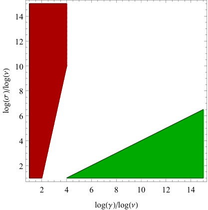
If the superfluid fraction is arbitrarily small, i.e., it goes to zero in the limit (3).
- •
The same holds for provided .
- •
If there is complete superfluidity, i.e., the superfluid fraction tends to 1.
The estimates that lead to these assertions are contained in Eqs. (5), (58) and (61) below. Figure 1 illustrates the parameter regions with and without superfluidity. (Note that we are concerned with asymptotic parameter regimes and the boundaries of the colored areas are not meant to indicate sharp transitions.)
We now describe briefly the organization of the paper. In the next Section 2 we first recall from [25] the description of the ground state properties of the Hamiltonian (1), in particular BEC, in terms of a Gross Pitaevskii functional. For this it is not necessary to assume the special potential (2), and we can state the results for an arbitrary nonnegative potential . The same holds in Section 2.2 where we show that superfluity in the ground state of many body Hamilonian is, in the large limit, equivalent to superfluity described in terms of the GP theory. In Section 3 we shall derive a closed formula for the superfluid fraction :
| (4) |
where is the minimizer of the GP energy functional.
A further general result (for an arbitrary nonnegative potential ) that we prove in Section 4 is an estimate for the deviation of the density from 1 in the sup norm :
| (5) |
When applied to this leads immediately to the sufficient criterion for complete superfluidity.
The absence of superfluity in the random potential for weak interactions and/or high density of scatterers is derived in Section 5.
2. BEC and superfluidity in the GP limit
2.1. BEC
An important fact about the Hamiltonian (1) that was proved in [25] is Bose-Einstein condensation in the ground state in the limit when and is fixed (GP limit), or does not grow too fast with . This holds in fact also if is replaced by an an arbitrary positive potential . The wave function of the condensate (eigenfunction to the highest eigenvalue of the one particle density matrix) is the minimizer of the Gross Pitaevskii (GP) energy functional
| (6) |
with the normalization . The minimizer is also the ground state of the mean field Hamiltonan
| (7) |
with eigenvalue . The average occupation of the one particle state in the many-body ground state of is with and the creation and annihilation operators for . Bose-Einstein condensation is expressed through the estimate
2.2. Superfluidity
To discuss superfluidity we modify the kinetic term of the Hamiltonian, replacing by with a velocity . We thus consider
| (9) |
on with periodic boundary conditions. Let denote its ground state energy and let denote the corresponding ground state energy of the modified GP functional
| (10) |
For small enough , has a unique minimizer, denoted by , and is equal to the ground state energy of the mean field Hamiltonian
| (11) |
Taking as trial function for the Hamiltonian we obtain
| (12) |
For the lower bound we write in the same way as Eq. (7) in [25]
| (13) |
We may now use the diamagnetic inequality ([27], p. 193) to bound an expectation value of the second term with respect to any wave function from below by the expectation value of
| (14) |
with respect to . Proceeding exactly as in [25], Eqs. (12)-(17), we can thus bound from below in terms of the mean field Hamiltonian with controlled errors terms, arriving at the lower bound for the ground state energy
| (15) |
We conclude that in the GP limit the superfluid fraction
| (16) |
is the same as the corresponding quantity derived from the GP energy, i.e.,
| (17) |
Note that in (16) the order in which the limits are taken is important in general. Using the GP minimizer for as a trial state for (10) we see that . Note also that the error term in (15) is independent of and uniformly small in for .
3. Proof of Eq. (4)
In this section we shall prove the formula (4) for the superfluid density. We start with the variational equation for which is
| (18) |
We multiply this by and take the imaginary part, to obtain
| (19) |
hence there exists a constant such that
| (20) |
Since
| (21) |
we actually see that . For small , has no zeroes, hence we can divide by and obtain
| (22) |
Since is, in fact, the derivative of the phase of , i.e, , we have, for a system with periodic boundary conditions,
| (23) |
for . For small enough , one has , and hence
| (24) |
4. Proof of Eq. (5)
We now derive the bound (5) which quantifies the deviation of the GP minimizer from a constant in terms of the average value of the random potential and the interaction strength.
Functions in the Sobolev space are continuous, and hence implies that for some . For such , we have
| (27) |
and hence
| (28) |
where is the sup norm and the -norm. We apply this to for an -normalized function . This gives
| (29) |
We further bound and hence find
| (30) |
In particular, for ,
| (31) |
For the GP minimizer satisfies (take as a trial function)
| (32) |
so
| (33) |
Since is close to with high probability, in the sense that the ratio converges to 1 in probability, we see that and hence also converges uniformly to 1 if as the parameters tend to . Thus the superfluid fraction is equal to 1 by Eq. (4).
5. Absence of superfluidity
If is any (measurable) subset of with length it follows from Eq. (4) and the Cauchy Schwarz inequality that
| (34) |
To prove that superfluidity is small we have therefore to identify subsets such that is small, while is not too small.
The random points split the intervall into subintervals of various lengths . The lengths are independent random variables11 1 Strictly speaking, because of the fixed endpoints 0 and 1, the interval lengths are not quite independent, but since the number of intervals is very large this does not affect the estimates. with identical probability distribution
| (35) |
We anticipate that intervals of small lengths have small occupation and shall therefore take
| (36) |
with a suitably chosen . The average length of is
| (37) |
In particular it tends to 1 if and only if .
With the notation
| (38) |
we define
| (39) |
Note that and also depend on but we have suppressed this in the notation for simplicity.
Our estimate on is based on estimates on the GP energy that were derived in [25]. These involve some auxiliary quantities that we now recall.
5.1. The energy between obstacles
The energy in an interval where the obstacles are placed only at the endpoints is given by suitable rescaling of the energy functional
| (40) |
with and . Let denote the auxiliary GP energy
| (41) |
The corresponding energy for an interval of length with mass , coupling constant and strength of the obstacle potential is then, by scaling,
| (42) |
We shall use the following bounds on that were derived in [25], Eqs. (32) and (41):
| (43) |
and
| (44) |
with constants and independent of and .
5.2. The interval density functional
With a mass distribution on intervals of various lengths we define an “interval density functional”, cf. [25], Eq. (42), as
| (45) |
with corresponding energy
| (46) |
This energy (denoted by ) is in [25], Theorem 3.1, proved to be the deterministic limit (in probability) of the GP energy under the conditions (3). The minimization problem (46) is conveniently treated by introducing a Lagrange multiplier for the normalization condition on . In [25], Eqs. (45)–(47), it is shown that
| (47) |
where denotes the function
| (48) |
Also . A further result derived in [25] is that the minimizing of the interval density functional is nonzero if and only if . We can therefore expect that the mass (38) is small in intervals such that and we shall make use of this in the following considerations.
5.3. Absence of superfluidity for
The first step is to split the GP energy , which is the minimum energy of (6) with in place of , into contributions from ‘large’ and ‘small’ intervals:
| (49) |
where
| (50) |
with a suitable to be chosen later, and (by (47) and (48))
| (51) |
Note that, since we have
| (52) |
for .
We estimate the sum over the small intervals using Eqs. (44) and (50):
| (53) |
For the sum over the large intervals we use (43) to estimate
| (54) |
Apart from the factor the right side is the GP energy for with normalization instead of . By simple scaling this is times the the GP energy with normalization 1 and replaced by , which in turn is not smaller than times . We can further estimate
| (55) |
and putting (53), (54) and (55) together we obtain
| (56) |
If , and tend to infinity under the constraints (3), the ratio stays bounded (in probability) according to Theorem 3.1 in [25]. Moreover, for if we have by (51) and (3)
| (57) |
For we thus arrive at an estimate for the mass in the small intervals:
| (58) |
and since, by (57),
| (59) |
we have shown that in probability if and the conditions (3) holds.
Now according to (34) the superfluid fraction is bounded from above by where is the total length of intervals of length . The latter converges in probability to the expectation value
| (60) |
provided the fluctuations remain small. For we have (by (51)) and the length converges to 1 as , while for the length stays bounded away from 0 because is . The fluctuations are . Hence the superfluid fraction tends to 0 in probability for .
5.4. The case
Here and we take . We need in any case , i.e., , which is compatible with the conditions (3). In the same way as above we obtain (58), this time with .
Since , however, the average length of the small intervals is now rather than as for . To exclude superfluidity we need
| (61) |
which holds for
| (62) |
This condition is still not sufficient, however, because the estimate can only be claimed to be true in probability as long as the fluctuations of the random variable are small compared to its average value, . A sufficient condition for this is that , which holds for . Altogether we conclude that the superfluid fraction tends to 0 in probability, if (62) together with hold.
6. Concluding remarks
We have studied superfluidity in the ground state of a one-dimensional model of bosons with a repulsive contact interaction and in a random potential generated by Poisson distributed point obstacles. In the Gross Pitaevskii (GP) limit this model always shows complete BEC, but depending on the parameters, superfluidity may or may not occur. In the course of the analysis we derived the closed formula (4) for the superfluid fraction, expressed in terms of the GP wave function.
The advantage of this model is that it is amenable to a rigorous mathematical analysis leading to unambiguous statements. It has its limitations: Nothing is claimed about positive temperatures and the proof of BEC requires that the ratio between the coupling constant for the interaction and the density tends to zero as . Nevertheless, to our knowledge this is the only model where a Bose glass phase in the sense of complete BEC but absence of superfluidity (cf. [9]) has been rigorously established so far.
Acknowledgements
This work is supported by the Austrian Science Fund (FWF) under project P 22929-N16.
References
- [1] O. Penrose, L. Onsager, Bose-Einstein Condensation and Liquid Helium, Phys. Rev. 104, 576–84 (1956).
- [2] A.J. Leggett, Superfluidity, Rev. Mod. Phys. 71, S318–S322 (1999).
- [3] P.C. Hohenberg and P.C. Martin, Microscopic theory of helium, Ann. Phys. (NY) 34, 291 (1965).
- [4] P. Sokol, Bose-Einstein Condensation in Liquid Helium, in: Bose-Einstein Condensation, A. Griffin, D.W. Snoke, S. Stringari, eds., Cambridge University Press, 51–85 (1995).
- [5] K. Huang, Bose-Einstein condensation and superfluidity, in: Bose-Einstein Condensation, A. Griffin, D.W. Stroke, S. Stringari, eds., Cambridge University Press, 31–50 (1995).
- [6] G.E. Astrakharchik, J. Boronat, J. Casulleras, and S. Giorgini, Superfluidity versus Bose-Einstein condensation in a Bose gas with disorder, Phys. Rev. A 66, 023603 (2002).
- [7] M. Kobayashi and M. Tsubota, Bose-Einstein condensation and superfluidity of a dilute Bose gas in a random potential, Phys. Rev. B 66, 174516 (2002).
- [8] V.I. Yukalov, R. Graham, Bose-Einstein condensed systems in random potentials, Phys. Rev. A 75, 023619 (2007).
- [9] V.I. Yukalov, E.P. Yukalova, K.V. Krutitsky, R. Graham, Bose-Einstein condensed gases in arbitrarily strong random potentials, Phys. Rev. A, 76, 053623 (2007).
- [10] E.H. Lieb, R. Seiringer, Proof of Bose-Einstein Condensation for Dilute Trapped Gases, Phys. Rev. Lett. 88, 170409-1–4 (2002).
- [11] E.H. Lieb, R. Seiringer, J. Yngvason, Superfluidity in Dilute Trapped Bose Gases, Phys. Rev. B 66, 134529 (2002).
- [12] H. Gimperlein, S. Wessel, J. Schmiedmayer, L. Santos, Ultracold Atoms in Optical lattices with Random One-Site Interactions, Phys. Rev. Lett. 95, 170401 (2005)
- [13] P. Lugan, P. Bouyer, A. Aspect, M. Lewenstein, L. Sanches-Palencia, Ultracold Bose Gases in 1D Disorder: From Lifshits Glass to Bose-Einstein Condensate, Phys. Rev. Lett. 98, 170403 (2007)
- [14] L. Fallani, C. Fort, M. Inguscio, Bose-Einstein Condensates in Disordered Potentials, Adv. At. Molec. Opt. Phys. 56, 119–159 (2008)
- [15] L. Sanches-Palencia, D. Clément, P. Lugan, P. Bouyer and A. Aspect, Disorder-induced trapping versus Anderson localization in Bose-Einstein condensates expanding in disordered potentials, New J. Phys. 10, 045019 (2008)
- [16] A.S. Pikovsky, D.L. Shepelyansky, Destruction of Anderson Localization by a Weak Nonlinearity, Phys. Rev. Lett. 100, 094101 (2008)
- [17] P. Lugan, A. Aspect, L. Sanches-Palencia, D. Delande, B. Grémaud, C.A. Müller, C. Miniatura, One-dimensional Anderson localization in certain correlated random potentials, Phys. Rev. A 80, 023605 (2009)
- [18] J. Radic, V. Bacic, D. Judic, M. Segev, H. Buljan, Anderson localization of a Tonks-Girardeau gas in potentials with controlled disorder, Phys. Rev. A 81, 063639 (2010)
- [19] I.L. Aleiner, B.L. Altshuler, G.V. Shlapnykov, A finite-temperature phase transition for disordered weakly interacting bosons in one dimension, Nature Phys. 6, 900–904 (2010)
- [20] L. Sanches-Palencia, M. Lewenstein, Disordered quantum gases under control, Nature Phys., 6, 87–95 (2010)
- [21] M. Piraud, P. Lugan, B. Bouyer, A. Aspect, and L. Sanches-Palencia, Localization of a matter wave packet in a disordered potential, Phys. Rev. A 83, 031603(R) (2011)
- [22] W.B. Cardoso, A.T. Avelar, D. Bazeia, Anderson localization of matter waves in chaotic potentials, Nonlin. Analysis 13, 755–763 (2012)
- [23] J. Stasinska, P. Massingnan, M. Bishop, J. Wehr, A. Sanpera and M. Lewenstein, The glass to superfluid transition in dirty bosons on a lattice, New J. Phys. 14, 043043 (2012)
- [24] M. Bishop, J. Wehr, Ground State Energy of Mean-field Model of Interacting Bosons in Bernoulli Potential, arXiv:1212.1487
- [25] R. Seiringer, J. Yngvason, V.A. Zagrebnov, Disordered Bose-Einstein condensates with interaction in one dimension, J. Stat. Mech. P11007 (2012).
- [26] R. Seiringer, J. Yngvason, V.A. Zagrebnov, Disordered Bose-Einstein condensates with interaction, in: XVIIth International Congress in Mathematical Physics, pp. 610–619, A. Jensen (ed.), World Scientific 2013. arXiv:1209.4046.
- [27] E.H. Lieb, W. Liniger, Exact Analysis of an Interacting Bose Gas. I., Phys. Rev. 130, 1605-1616 (1963)
- [28] E.H. Lieb, M. Loss, Analysis, 2nd Edition, American Mathematical Society, 2001.