跳到论文正文
W Papers独立论文阅读器 arXiv:1407.3152 论文正文 计算阅读时间 · 0%
引用这篇论文根据当前论文元数据生成,正式投稿前建议核对。


License: arXiv.org perpetual non-exclusive license
arXiv:1407.3152v1 [stat.ME] 11 Jul 2014

Maximum Smoothed Likelihood Component Density Estimation in Mixture Models with Known Mixing Proportions

Tao Yu Note: Supported in part by NUS Grant R-155-000-134-112 and R-155-000-123-112.    Pengfei Li Note: Supported in part by the Natural Sciences and Engineering Research Council of Canada, and by a startup grant from the University of Waterloo.    Jing Qin Affiliation: National University of Singapore, University of Waterloo, Affiliation: and National Institutes of Health
August 24, 2026
Abstract

In this paper, we propose a maximum smoothed likelihood method to estimate the component density functions of mixture models, in which the mixing proportions are known and may differ among observations. The proposed estimates maximize a smoothed log likelihood function and inherit all the important properties of probability density functions. A majorization-minimization algorithm is suggested to compute the proposed estimates numerically. In theory, we show that starting from any initial value, this algorithm increases the smoothed likelihood function and further leads to estimates that maximize the smoothed likelihood function. This indicates the convergence of the algorithm. Furthermore, we theoretically establish the asymptotic convergence rate of our proposed estimators. An adaptive procedure is suggested to choose the bandwidths in our estimation procedure. Simulation studies show that the proposed method is more efficient than the existing method in terms of integrated squared errors. A real data example is further analyzed.

Key words and phrases: EM-like Algorithm; Empirical process; M-estimators; Majorization-minimization algorithm; Mixture data; Smoothed likelihood function.

Running title: MSL Component Density Estimation in Mixture Models.

1 Introduction

In this paper, we consider the data with the following mixture structure. Let {Xi,𝜶i}\{X_{i},\mbox{\boldmath$\alpha$}_{i}\}, i=1,…,ni=1,\ldots,n, be independent and identically distributed (i.i.d.) copies of {X,𝜶}\{X,\mbox{\boldmath$\alpha$}\}. For every i=1,…,ni=1,\ldots,n, XiX_{i} comes from one of the MM subpopulations with probability density functions (pdfs) f1​(x),…,fM​(x)f_{1}(x),\ldots,f_{M}(x). Denote by αi,j\alpha_{i,j} the probability that XiX_{i} is from the jjth subpopulation and let 𝜶i=(αi,1,…,αi,M)τ\mbox{\boldmath$\alpha$}_{i}=(\alpha_{i,1},\ldots,\alpha_{i,M})^{\tau}. Clearly αi,j≥0\alpha_{i,j}\geq 0 and ∑j=1Mαi,j=1\sum_{j=1}^{M}\alpha_{i,j}=1. In summary, the pdf of XiX_{i} conditioning on 𝜶i\mbox{\boldmath$\alpha$}_{i} is given by

Xi|𝜶i∼∑j=1Mαi,j​fj​(x).\displaystyle X_{i}|\mbox{\boldmath$\alpha$}_{i}\sim\sum_{j=1}^{M}\alpha_{i,j}f_{j}(x). (1)

Practically, 𝜶i\mbox{\boldmath$\alpha$}_{i} is known, observable, or can be reliably estimated from other sources. That is, conditioning on 𝜶i\mbox{\boldmath$\alpha$}_{i}, XiX_{i} follows a mixture model with known mixing proportions. Our main interest in this paper is to estimate f1​(x),…,fM​(x)f_{1}(x),\ldots,f_{M}(x) nonparametrically.

Recently, data of the mixture structure in (1) have been more and more frequently identified in the literature and in practice. Acar and Sun (2013) provided one example of such data. In the genetic association study of single nucleotide polymorphisms (SNPs), the corresponding genotypes of SNPs are usually not deterministic; in the resultant data, they are typically delivered as genotype probabilities from various genotype calling or imputation algorithms (see for example Li et al. 2009 and Carvalho et al. 2010). Ma and Wang (2012) summarized two types of genetic epidemiology studies under which mixture data of such kind are collected. These studies are kin-cohort studies (Wang et al. 2008) and quantitative trait locus studies (Lander and Botstein 1989; Wu et al. 2007); see also Wang et al. (2012) and the references therein. Section 7 also gives an example of such data in the malaria study. More examples and the corresponding statistical research can be founded in Ma et al. (2011), Qin et al. (2014), and the references therein.

With the data of the mixture structure in (1), statistical methods for estimating the component cumulative distribution functions (cdfs) have been established in the literature. A comprehensive overview of these developments is as follows. Ma and Wang (2012) pointed out that the classic maximum empirical likelihood estimators of these component cdfs are either highly inefficient or inconsistent. They proposed a class of weighted least square estimators. Wang et al. (2012) and Ma and Wang (2014) proposed consistent and efficient nonparametric estimators based on estimating equations for the component cdfs when the data are censored. Qin et al. (2014) considered another class of estimators for the component cdfs by maximizing the binomial likelihood. Their method can be applied to data with censored or a non-censored structure. We observe that all these works were focused on the estimation of cdfs and assumed 𝜶i\mbox{\boldmath$\alpha$}_{i} to be a discrete random vector.

The estimation of the pdfs are less addressed in the literature. As far as we are aware, to date Ma et al. (2011) is the only existing reference that considered the component density estimation under the setup of model (1). They proposed a family of kernel-based weighted least squares estimators for the component pdfs under the assumption that 𝜶i\mbox{\boldmath$\alpha$}_{i} is continuous. However, to the best of our knowledge, there are two limitations in their approach: (1) the resultant estimates do not inherit the nonnegativity property of a regular density function; as is well known, such a property is often important in many downstream density-based studies. In that paper, though authors have discussed an EM-like algorithm to achieve nonnegative component density estimates, the corresponding theoretical properties as well as the numerical performance of these estimates were not studied yet. (2) When dealing with some practical problems, this method does not make full use of the data and therefore the resultant density estimation may not be as efficient. We refer to the end of Section 6 for an example and further discussion.

In this paper, we consider maximum smoothed likelihood (Eggermont and Lariccia 2001, Chapter 4) estimators for f1,…,fMf_{1},\ldots,f_{M}, namely f^1,…,f^M\widehat{f}_{1},\ldots,\widehat{f}_{M}, which maximize a smoothed likelihood function and inherit all the important properties of pdfs. Our method can handle data with 𝜶i\mbox{\boldmath$\alpha$}_{i}’s continuous or discrete. We also propose a majorization-minimization algorithm that computes these density estimates numerically. This algorithm incorporates similar ideas as Levine et al. (2011) and the EM-like algorithm (Hall et al. 2005). We show that under finite samples, starting from any initial value, this algorithm not only increases the smoothed likelihood function but also leads to estimates that maximize the smoothed likelihood function.

Another main contribution of this paper is to establish the L1L_{1} asymptotic consistency and the corresponding convergence rate for our density estimates. Because of the properties (see Section 4) of the non-linear operator “𝒩h\mbox{$\mathcal{N}$}_{h}” defined in Section 2 and the complicated form of the smoothed log-likelihood function, the development of the asymptotic theories for the nonparametric density estimates under the framework of mixture model is technically challenging and still lacking in the literature. We solve this problem by employing the advanced theories in empirical process (see van der Vaart and Wellner 1996, Kosorok 2008, and the references therein). We expect that the technical tools established in this paper may benefit the future study on the asymptotic theories of the nonparametric density estimates for mixture model of other kinds; see for example Levine et al. (2011).

The rest of the paper is organized as follows. Section 2 presents our proposed density estimates based on smoothed likelihood principal. Section 3 suggests a majorization-minimization algorithm to numerically compute these density estimates, and establishes the finite-sample convergence properties of this algorithm. Section 4 studies the asymptotic behaviors of our density estimators. Section 5 proposes a bandwidth selection procedure that is easily imbedded into the majorization-minimization algorithm. Section 6 conducts simulation studies, which show that the proposed method is more efficient than existing methods in terms of integrated square error. Section 7 applies our method to a real data example. The technical details are relegated to the Appendix.

2 Maximum Smoothed Likelihood Estimation

With the observed data {Xi,𝜶i}i=1n\{X_{i},\mbox{\boldmath$\alpha$}_{i}\}_{i=1}^{n} from Model (1), we propose a maximum smoothed likelihood method for estimating f1,…,fMf_{1},\ldots,f_{M}. We consider the set of functions

𝒞={(f1,…,fM):fj is a pdf ,j=1,…,M}.\displaystyle\mathcal{C}=\left\{(f_{1},\ldots,f_{M}):f_{j}\mbox{ is a pdf },j=1,\ldots,M\right\}.

Furthermore, we assume that fjf_{j}’s have the common support SxS_{x}.

Given Model (1) and observations {Xi,𝜶i}i=1n\{X_{i},\mbox{\boldmath$\alpha$}_{i}\}_{i=1}^{n}, the conditional log-likelihood can be written as

l~n​(f1,…,fM)=∑i=1nlog⁡{∑j=1Mαi,j​fj​(Xi)}.\displaystyle\widetilde{l}_{n}(f_{1},\ldots,f_{M})=\sum_{i=1}^{n}\log\left\{\ \sum_{j=1}^{M}\alpha_{i,j}f_{j}(X_{i})\right\}.

However, as is well known, this log-likelihood function is unbounded in 𝒞\mathcal{C}; see page 25 in Silverman (1986) and page 111 in Eggermont and Lariccia (2001). Therefore, the corresponding maximum likelihood estimates do not exist. This unboundedness problem can be solved by incorporating the smoothed likelihood approach (Eggermont and Lariccia, 1995, Groeneboom et al.  2010, Yu et al. 2014, and the references therein). Specifically, we define the smoothed log-likelihood of f1​(x),…,fM​(x)f_{1}(x),\ldots,f_{M}(x) to be

ln​(f1,…,fM)=∑i=1nlog⁡{∑j=1Mαi,j​𝒩hj​fj​(Xi)},l_{n}(f_{1},\ldots,f_{M})=\sum_{i=1}^{n}\log\left\{\sum_{j=1}^{M}\alpha_{i,j}\mbox{$\mathcal{N}$}_{h_{j}}f_{j}(X_{i})\right\}, (2)

where 𝒩h​f​(x)\mbox{$\mathcal{N}$}_{h}f(x) is the nonlinear smoothing operator for a density function ff, represented by

𝒩h​f​(x)\displaystyle\mbox{$\mathcal{N}$}_{h}f(x) =\displaystyle= exp⁡{∫ℝKh​(u−x)​log⁡f⁡(u)​𝑑u}.\displaystyle\exp\left\{\int_{\mathbb{R}}K_{h}(u-x)\log f(u)du\right\}. (3)

Here Kh​(x)=1h​K​(x/h)K_{h}(x)=\frac{1}{h}K(x/h), K⁡(⋅)K(\cdot) is a kernel function supported on [−L,L][-L,L], and hh is the bandwidth for the nonlinear smoothing operator. By convention, we define 0​log⁡(0)=00\log(0)=0, log⁡(0)=−∞\log(0)=-\infty, and exp⁡(−∞)=0\exp(-\infty)=0.

Our proposed maximum smoothed likelihood estimators for f1,…,fMf_{1},\ldots,f_{M} are given by

(f^1,…,f^M)=argmax(f1,…,fM)∈𝒞​ln​(f1,…,fM).\displaystyle(\widehat{f}_{1},\ldots,\widehat{f}_{M})=\mbox{argmax}_{(f_{1},\ldots,f_{M})\in\mathcal{C}}l_{n}(f_{1},\ldots,f_{M}). (4)

We observe that the smoothed likelihood function defined in (2) has the following properties. First, based on Lemma 3.1 (iii) of Eggermont (1999), ln​(⋅)l_{n}(\cdot) is concave in 𝒞\mathcal{C}, and 𝒞\mathcal{C} is a convex set of functions. Second, if the kernel function K⁡(t)K(t) is bounded and hj>0h_{j}>0, j=1,…,Mj=1,\ldots,M are fixed, then ln​(⋅)l_{n}(\cdot) is also bounded in 𝒞\mathcal{C}, since for every xx and (f1,…,fM)∈𝒞(f_{1},\ldots,f_{M})\in\mathcal{C},

𝒩hj​fj​(x)\displaystyle\mbox{$\mathcal{N}$}_{h_{j}}f_{j}(x) ≤\displaystyle\leq exp⁡[log⁡{∫ℝKh​(u−x)​f​(u)​𝑑u}]≤suptK⁡(t)/hj.\displaystyle\exp\left[\log\left\{\int_{\mathbb{R}}K_{h}(u-x)f(u)du\right\}\right]\leq\sup_{t}K(t)/h_{j}.

Therefore, the maximizer of ln​(⋅)l_{n}(\cdot) exists, i.e., the optimization problem (4) is well defined. Furthermore, if we assume that for every j=1,…,Mj=1,\ldots,M, the XiX_{i}’s corresponding to αi,j>0\alpha_{i,j}>0 are dense in SxS_{x}, then ln​(⋅)l_{n}(\cdot) is strictly concave in 𝒞\mathcal{C} and thus the solution to the optimization problem (4) is unique. Here, “dense” means for every j=1,…,Mj=1,\ldots,M, and x∈Sxx\in S_{x}, the interval [x−L​hj,x+L​hj][x-Lh_{j},x+Lh_{j}] contains at least one observation XiX_{i}, such that the corresponding αi,j>0\alpha_{i,j}>0.

3 The majorization-minimization algorithm

In this section, we propose an algorithm that numerically calculates f^1,…,f^M\widehat{f}_{1},\ldots,\widehat{f}_{M} with given bandwidths h1,…,hMh_{1},\ldots,h_{M} and study the finite-sample convergence property of this algorithm. The proposed algorithm, called the majorization-minimization algorithm, is in spirit similar to the majorization-minimization algorithm in Levine et al. (2011). To facilitate our theoretical development, we define the majorization-minimization updating operator 𝒢\mathcal{G} on 𝒞\mathcal{C} as follows. For any (f1,…,fM)∈𝒞(f_{1},\ldots,f_{M})\in\mathcal{C}, let

𝒢⁡(f1,…,fM)=(f1𝒢,…,fM𝒢),\displaystyle\mathcal{G}(f_{1},\ldots,f_{M})=(f_{1}^{\mathcal{G}},\ldots,f_{M}^{\mathcal{G}}), (5)

where

fj𝒢​(x)\displaystyle f_{j}^{\mathcal{G}}(x) =\displaystyle= ∑i=1nwi,j​Khj​(x−Xi)∑i=1nwi,j,\displaystyle\frac{\sum_{i=1}^{n}w_{i,j}K_{h_{j}}(x-X_{i})}{\sum_{i=1}^{n}w_{i,j}},
with wi,j\displaystyle\mbox{with }\quad w_{i,j} =\displaystyle= αi,j​𝒩hj​fj​(Xi)∑k=1Mαi,k​𝒩hk​fk​(Xi).\displaystyle\frac{\alpha_{i,j}\mbox{$\mathcal{N}$}_{h_{j}}f_{j}(X_{i})}{\sum_{k=1}^{M}\alpha_{i,k}\mbox{$\mathcal{N}$}_{h_{k}}f_{k}(X_{i})}. (6)

We first show that 𝒢\mathcal{G} is capable of increasing the smoothed log-likelihood function lnl_{n} in every step of updating.

Theorem 1.

For every (f1,…,fM)∈𝒞(f_{1},\ldots,f_{M})\in\mathcal{C}, we have ln​(𝒢⁡(f1,…,fM))≥ln​(f1,…,fM)l_{n}\left(\mathcal{G}(f_{1},\ldots,f_{M})\right)\geq l_{n}\left(f_{1},\ldots,f_{M}\right).

Theorem 1 immediately leads to our proposed majorization-minimization algorithm as follows. Given initial values (f10,…,fM0)∈𝒞(f_{1}^{0},\ldots,f_{M}^{0})\in\mathcal{C}, for s=0,1,2,⋯s=0,1,2,\cdots, we iteratively update from (f1s,…,fMs)(f_{1}^{s},\ldots,f_{M}^{s}) to (f1s+1,…,fMs+1)(f_{1}^{s+1},\ldots,f_{M}^{s+1}) as

(f1s+1,…,fMs+1)=𝒢⁡(f1s,…,fMs).(f_{1}^{s+1},\ldots,f_{M}^{s+1})=\mathcal{G}(f_{1}^{s},\ldots,f_{M}^{s}).

Clearly, Theorem 1 above ensures that for every s=0,1,…s=0,1,\ldots, we have ln​(f1s+1,…,fMs+1)≥ln​(f1s,…,fMs)l_{n}\left(f_{1}^{s+1},\ldots,f_{M}^{s+1}\right)\geq l_{n}\left(f_{1}^{s},\ldots,f_{M}^{s}\right). Furthermore, since for any (f1,…,fM)∈𝒞(f_{1},\ldots,f_{M})\in\mathcal{C}, 𝒢⁡(f1,…,fM)\mathcal{G}(f_{1},\ldots,f_{M}) belongs to the class of functions ℱn\mathcal{F}_{n}:

ℱn\displaystyle\mathcal{F}_{n} =\displaystyle= {(f1,…,fM):fj(x)=∑i=1nwi,j​Khj​(x−Xi)∑i=1nwi,j;0≤wi,j≤1},\displaystyle\left\{(f_{1},\ldots,f_{M}):f_{j}(x)=\frac{\sum_{i=1}^{n}w_{i,j}K_{h_{j}}(x-X_{i})}{\sum_{i=1}^{n}w_{i,j}};0\leq w_{i,j}\leq 1\right\}, (7)

therefore, (f1s,…,fMs)∈ℱn(f_{1}^{s},\ldots,f_{M}^{s})\in\mathcal{F}_{n} for s≥1s\geq 1. Next, we study the finite-sample convergence property of this majorization-minimization algorithm; we observe that the technical development for such a convergence property is nontrivial. We first present a sufficient and necessary condition under which (f^1,…,f^M)∈𝒞(\widehat{f}_{1},\ldots,\widehat{f}_{M})\in\mathcal{C} is a solution of the optimization problem (4).

Theorem 2.

Assume for every j=1,…,Mj=1,\ldots,M, ∑i=1nαi,j>0\sum_{i=1}^{n}\alpha_{i,j}>0. Consider (f^1,…,f^M)∈𝒞(\widehat{f}_{1},\ldots,\widehat{f}_{M})\in\mathcal{C}, then

ln​(f^1,…,f^M)=sup(f1,…,fM)∈𝒞ln​(f1,…,fM)\displaystyle l_{n}(\widehat{f}_{1},\ldots,\widehat{f}_{M})=\sup_{(f_{1},\ldots,f_{M})\in\mathcal{C}}l_{n}(f_{1},\ldots,f_{M})

if and only if (f^1,…,f^M)=𝒢⁡(f^1,…,f^M)(\widehat{f}_{1},\ldots,\widehat{f}_{M})=\mathcal{G}(\widehat{f}_{1},\ldots,\widehat{f}_{M}) almost surely under the Lebesgue measure.

The following corollary is resulted from an immediately application of Theorem 2; the straightforward proof is omitted.

Corollary 1.

Assume for every j=1,…,Mj=1,\ldots,M, ∑i=1nαi,j>0\sum_{i=1}^{n}\alpha_{i,j}>0. Let (f^1,…,f^M)(\widehat{f}_{1},\ldots,\widehat{f}_{M}) be a solution of the optimization problem (4), then (f^1,…,f^M)∈ℱn(\widehat{f}_{1},\ldots,\widehat{f}_{M})\in\mathcal{F}_{n} almost surely under the Lebesgue measure.

Corollary 1 benefits our subsequent technical development of the asymptotic theories for f^1,…,f^M\widehat{f}_{1},\ldots,\widehat{f}_{M} in Section 4. It indicates that the solution of (4) is equivalent to the solution of

(f^1,…,f^M)=argmax(f1,…,fM)∈ℱn​ln​(f1,…,fM),\displaystyle(\widehat{f}_{1},\ldots,\widehat{f}_{M})=\mbox{argmax}_{(f_{1},\ldots,f_{M})\in\mathcal{F}_{n}}l_{n}(f_{1},\ldots,f_{M}), (8)

as long as the stated condition ∑i=1nαi,j>0\sum_{i=1}^{n}\alpha_{i,j}>0 for every jj is satisfied. This condition is quite reasonable since if ∑i=1nαi,j=0\sum_{i=1}^{n}\alpha_{i,j}=0 for some jj then the jjth subpopulation does not appear in the data and we can delete the corresponding fj​(x)f_{j}(x) from the mixture model (1). Therefore, developing the asymptotic theories for f^1,…,f^M\widehat{f}_{1},\ldots,\widehat{f}_{M} from (4) is equivalent to developing those from (8).

Based on Theorem 2, we show the convergence of the updating sequence ln​(f1s,…,fMs)l_{n}\left(f_{1}^{s},\ldots,f_{M}^{s}\right) to its global maximum, which implies the convergence of the proposed majorization-minimization algorithm.

Theorem 3.

Assume suptK⁡(t)<∞\sup_{t}K(t)<\infty. Then, we have

lims→∞ln​(f1s,…,fMs)=ln​(f^1,…,f^M),\displaystyle\lim_{s\to\infty}l_{n}(f_{1}^{s},\ldots,f_{M}^{s})=l_{n}(\widehat{f}_{1},\ldots,\widehat{f}_{M}),

where (f^1,…,f^M)∈ℱn(\widehat{f}_{1},\ldots,\widehat{f}_{M})\in\mathcal{F}_{n} is a solution of the optimization problem (4).

Based on Theorem 3, if we don’t impose further conditions on the data, ln​(⋅)l_{n}(\cdot) is not necessarily strictly concave. Therefore, we can only show that the updating sequence ln​(f1s,…,fMs)l_{n}(f_{1}^{s},\ldots,f_{M}^{s}) converges to the maximum of ln​(f1,…,fM)l_{n}(f_{1},\ldots,f_{M}). Note that this does not guarantee the convergence of (f1s,…,fMs)(f_{1}^{s},\ldots,f_{M}^{s}) to (f^1,…,f^M)(\widehat{f}_{1},\ldots,\widehat{f}_{M}), i.e., the maximizer of ln​(f1,…,fM)l_{n}(f_{1},\ldots,f_{M}), because such a maximizer may not be uniquely defined. Instead, referring to the proof of this theorem, we have shown that there exists at least a subsequence of (f1s,…,fMs)(f_{1}^{s},\ldots,f_{M}^{s}) converging to a maximizer of ln​(f1,…,fM)l_{n}(f_{1},\ldots,f_{M}). Furthermore, if we impose some technical condition such that ln​(⋅)l_{n}(\cdot) is strictly concave, (f^1,…,f^M)(\widehat{f}_{1},\ldots,\widehat{f}_{M}) is then uniquely defined by (4). Immediately, we can show lims→∞(f1s,…,fMs)=(f^1,…,f^M)\lim_{s\to\infty}(f_{1}^{s},\ldots,f_{M}^{s})=(\widehat{f}_{1},\ldots,\widehat{f}_{M}) for every x∈Sxx\in S_{x}. We refer to the discussion at the end of Section 2 for a sufficient condition so that lnl_{n} is strictly concave in 𝒞\mathcal{C}.

We end this section with the following remark about the proposed majorization-minimization algorithm above.

Remark 1.

Ma et al. (2011) discussed an EM-like algorithm in their discussion section to obtain nonnegative component density estimates. In particular, they suggested defining

wi,j=αi,j​fj​(Xi)∑k=1Mαi,k​fk​(Xi),w_{i,j}=\frac{\alpha_{i,j}f_{j}(X_{i})}{\sum_{k=1}^{M}\alpha_{i,k}f_{k}(X_{i})},

and using a similar way as (5) to update the resultant density estimates in their paper. Yet, the corresponding theoretical properties as well as the numerical performance of these estimates are left unknown. As commented by Levine et al. (2011), algorithms of this kind do not minimize/maximize any particular objective function; this may impose difficulty in the subsequent technical development. We refer to Levine et al. (2011) for more discussion of such a method.

4 Asymptotic Properties for (f^1,…,f^M)(\widehat{f}_{1},\ldots,\widehat{f}_{M})

In this section, we investigate the asymptotic behaviors of (f^1,…,f^M)(\widehat{f}_{1},\ldots,\widehat{f}_{M}) given in (4). First, we consider the consistency of p^​(x,𝜶)=∑j=1Mαj​𝒩hj​f^j​(x)\widehat{p}(x,\mbox{\boldmath$\alpha$})=\sum_{j=1}^{M}\alpha_{j}\mbox{$\mathcal{N}$}_{h_{j}}\widehat{f}_{j}(x) under the Hellinger distance, where the Hellinger distance between two non-negative functions g1​(ω)g_{1}(\omega) and g2​(ω)g_{2}(\omega) is defined to be

d⁡(g1,g2)=[∫Ω{g11/2​(ω)−g21/2​(ω)}2​𝑑μ]1/2.\displaystyle d(g_{1},g_{2})=\left[\int_{\Omega}\left\{g_{1}^{1/2}(\omega)-g_{2}^{1/2}(\omega)\right\}^{2}d\mu\right]^{1/2}.

where g1,g2g_{1},g_{2} are functions defined on Ω\Omega, μ\mu is a measure on Ω\Omega.

Theorem 4.

Assume Conditions 1–3. Then for any ϑ>0\vartheta>0, we have

d⁡(γ​p^,γ​p~0)=Op​(h0.5)+Op​(n−0.5+ϑ​h−0.5).\displaystyle d(\gamma\widehat{p},\gamma\widetilde{p}_{0})=O_{p}(h^{0.5})+O_{p}(n^{-0.5+\vartheta}h^{-0.5}).

where γ⁡(𝛂)\gamma(\mbox{\boldmath$\alpha$}) is the marginal density of 𝛂\alpha, p~0​(x,𝛂)=∑j=1Mαj​f0,j​(x)\widetilde{p}_{0}(x,\mbox{\boldmath$\alpha$})=\sum_{j=1}^{M}\alpha_{j}f_{0,j}(x) is the conditional density of XX given 𝛂\alpha, and f0,j​(x)f_{0,j}(x), j=1,…,Mj=1,\ldots,M, denote the true values of fj​(x)f_{j}(x).

Next we establish the asymptotic convergence rate for 𝒩hj​f^j\mbox{$\mathcal{N}$}_{h_{j}}\widehat{f}_{j}, j=1,…,Mj=1,\ldots,M under the L1L_{1}-distance. The proof of this theorem heavily replies on the results given in Theorem 4.

Theorem 5.

Assume Conditions 1–4 in Appendix B. For every ϑ>0\vartheta>0 and j=1,…,Mj=1,\ldots,M, we have

∫ℝ|𝒩hj​f^j​(x)−f0,j​(x)|​𝑑x=Op​(h1/2)+Op​(n−0.5+ϑ​h−0.5).\displaystyle\int_{\mathbb{R}}|\mbox{$\mathcal{N}$}_{h_{j}}\widehat{f}_{j}(x)-f_{0,j}(x)|dx=O_{p}(h^{1/2})+O_{p}(n^{-0.5+\vartheta}h^{-0.5}).

Last, we establish the L1L_{1} convergence of f^j​(x)\widehat{f}_{j}(x). We observe that the results by Theorems 2 and 5 play key roles in the proof.

Theorem 6.

Assume Conditions 1–4 in Appendix B. For any ϑ>0\vartheta>0, we have

∫ℝ|f^j(x)−f0,j(x)|dx=Op(h1/2)+Op(n−0.5+ϑh−0.5),j=1,…,M.\displaystyle\int_{\mathbb{R}}|\widehat{f}_{j}(x)-f_{0,j}(x)|dx=O_{p}(h^{1/2})+O_{p}(n^{-0.5+\vartheta}h^{-0.5}),~~j=1,\ldots,M.

For presentational continuity, we have organized the technical conditions and long proofs of Theorems 4–6 in Appendix B. As observed in Appendix B, the theoretical developments for these theorems are technically challenging. The main obstacles are due to the following undesirable properties of 𝒩h​f​(x)\mbox{$\mathcal{N}$}_{h}f(x) with f⁡(x)f(x) being an arbitrary pdf.

Firstly, 𝒩h​f​(x)\mbox{$\mathcal{N}$}_{h}f(x) is neither a density nor necessarily sufficiently close to the corresponding f⁡(x)f(x). Therefore, the well developed empirical process theories and technics for M-estimators in density estimation (see for example Section 3.4.1 in van der Vaart and Wellner 1996) is not directly applicable.

Secondly, 𝒩h​f​(x)\mbox{$\mathcal{N}$}_{h}f(x) introduces significant bias on the boundary of the support of f⁡(x)f(x). For example, if f⁡(x)f(x) is supported on [c1,c2][c_{1},c_{2}], then 𝒩h​f​(x)\mbox{$\mathcal{N}$}_{h}f(x) is supported on [c1+L​h,c2−L​h][c_{1}+Lh,c_{2}-Lh]. That is 𝒩h​f​(x)=0\mbox{$\mathcal{N}$}_{h}f(x)=0 when x∈[c1,c1+Lh)∪(c2−Lh,c2]x\in[c_{1},c_{1}+Lh)\cup(c_{2}-Lh,c_{2}]. Here [−L,L][-L,L] is the support for the kernel function K⁡(x)K(x).

These two properties of 𝒩h​f​(x)\mbox{$\mathcal{N}$}_{h}f(x) significantly challenge our technical development. So far, we can only show the asymptotic behaviours of p^​(x)\widehat{p}(x), 𝒩hj​f^j​(x)\mbox{$\mathcal{N}$}_{h_{j}}\widehat{f}_{j}(x), and f^j​(x)\widehat{f}_{j}(x) as those given in Theorems 4, 5 and 6. The convergence rate given in Theorems 5 and 6 may not be the optimal. There is some room to improve. However, because of these two properties of “𝒩h\mbox{$\mathcal{N}$}_{h}”, we conjecture that Op​(h0.5)O_{p}(h^{0.5}) is the best rate achievable by d⁡(γ​p^,γ​p~0)d(\gamma\widehat{p},\gamma\widetilde{p}_{0}) under the assumption that f0,j​(x)f_{0,j}(x)’s are supported on a compact support. The intuition is as follows. Consider the extreme case that even though f^j​(x)\widehat{f}_{j}(x)’s are estimated ideally well, f^j​(x)=f0,j​(x)\widehat{f}_{j}(x)=f_{0,j}(x) say, one can show that the best rate for d⁡(γ​p^,γ​p~0)d(\gamma\widehat{p},\gamma\widetilde{p}_{0}) is still bounded by Op​(h0.5)O_{p}(h^{0.5}).

5 Bandwidth Selection

The maximum smoothed likelihood estimates f^1,…,f^M\widehat{f}_{1},\ldots,\widehat{f}_{M} depend on the choice of the bandwidths h1,…,hMh_{1},\ldots,h_{M}. We suggest an algorithm that embeds the selection of the bandwidth h1,…,hMh_{1},\ldots,h_{M} into the updating steps of the majorization-minimization algorithm suggested in Section 3.

Let njn_{j} be the positive integer closest to ∑i=1nαi,j\sum_{i=1}^{n}\alpha_{i,j}, which serves as an estimate of the average number of observations from the jjth population. Given initial values (f10,…,fM0)(f_{1}^{0},\ldots,f_{M}^{0}) and initial bandwidths (h10,…,hM0)(h_{1}^{0},\ldots,h_{M}^{0}), for s=0,1,2,⋯s=0,1,2,\cdots. We update (f1s,…,fMs)(f_{1}^{s},\ldots,f_{M}^{s}) and (h1s,…,hMs)(h_{1}^{s},\ldots,h_{M}^{s}) as follows.

  1. Step 1. For every i=1,…,ni=1,\ldots,n and j=1,…,Mj=1,\ldots,M, let

    wi,js=αi​j​𝒩hjs​fjs​(Xi)∑j=1Mαi​j​𝒩hjs​fjs​(Xi).w_{i,j}^{s}=\frac{\alpha_{ij}\mbox{$\mathcal{N}$}_{h_{j}^{s}}f_{j}^{s}(X_{i})}{\sum_{j=1}^{M}\alpha_{ij}\mbox{$\mathcal{N}$}_{h_{j}^{s}}f_{j}^{s}(X_{i})}.
  2. Step 2. Sort wi,jsw_{i,j}^{s}: w(1),j(s)≥w(2),js≥⋯≥w(n),jsw_{(1),j}^{(s)}\geq w_{(2),j}^{s}\geq\cdots\geq w_{(n),j}^{s}. Let Sjs={Xi:wi,j≥w(nj),js}S_{j}^{s}=\{X_{i}:w_{i,j}\geq w_{(n_{j}),j}^{s}\}. Treating the observations in SjsS_{j}^{s} as from a single population, we apply available bandwidth selection method for classical kernel density estimate to choose hjh_{j}. Denote by hjs+1h_{j}^{s+1} the resultant bandwidth.

  3. Step 3. Let

    fjs+1​(x)=∑i=1nwi​js​Khjs+1​(x−Xi)∑i=1nwi​js.f_{j}^{s+1}(x)=\frac{\sum_{i=1}^{n}w_{ij}^{s}K_{h_{j}^{s+1}}(x-X_{i})}{\sum_{i=1}^{n}w_{ij}^{s}}.

The philosophy of the above bandwidth selection step (i.e. Step 2) is as follows. In fact, SjsS_{j}^{s} collects the njn_{j} observations most likely coming from the jjth population based on the preceding iteration. Therefore, we use these observations to select the bandwidth for the corresponding density estimates in the current iteration.

When implementing this algorithm in our numerical studies, we use the quartic kernel, which was also used by Ma et al. (2011). The initial density (f10,…,fM0)(f_{1}^{0},\ldots,f_{M}^{0}) is randomly chosen from ℱn\mathcal{F}_{n}, i.e., the corresponding weights wi,jw_{i,j} are randomly generated from the uniform distribution over [0,1]. In the bandwidth selection step (i.e. Step 2), once SjsS_{j}^{s} is obtained, we use R function dpik() to update the bandwidths hjs+1h_{j}^{s+1}, j=1,…,Mj=1,\ldots,M. dpik() in the R package KernSmooth is implemented by Wand and Matt (publicly available at http://CRAN.R-project.org/package=KernSmooth). This package is based on the kernel methods in Wand and Jones (1996). Furthermore, the initial bandwidths are set as hj0=h0h_{j}^{0}=h^{0} for every j=1,…,Mj=1,\ldots,M, where h0h^{0} is the output of dpik() based on all the observations X1,…,XnX_{1},\ldots,X_{n}. We iterate Steps 1–3 until the change of the smoothed likelihood ln​(f1,…,fM)l_{n}(f_{1},\ldots,f_{M}) is smaller than a tolerance value 10−510^{-5} in each iteration.

In our numerical studies, we observe that this algorithm converges fast. For example, consider the real data example in Section 7. Setting the random seed set as “123456”, the bandwidths do not change up to 6th decimal point in two iterations; the change of lnl_{n} is less than 10−510^{-5} in another 59 iterations. We have also experimented with other random seeds. The results are very similar. In addition, the resultant estimates for f1,…,fMf_{1},\ldots,f_{M} are independent of the choice of (f10,…,fM0)(f_{1}^{0},\ldots,f_{M}^{0}).

6 Simulation Study

We use the following simulation examples to examine the numerical performance of our density estimates. We consider three “Studies”. Studies I and II adopt the same setup as those in Ma et al. (2011) so that we can compare the results by our method with those in that paper. Study III mimics the real data example given in Section 7.

In the first study (Study I), we generate data using two populations, i.e., M=2M=2. Both populations have a standard normal distribution, so that f0,1=f0,2=ϕ0f_{0,1}=f_{0,2}=\phi_{0}, where ϕ0\phi_{0} denotes the pdf of the standard normal distribution. We generate X1,…,XnX_{1},\ldots,X_{n} with n=400n=400. For every XiX_{i}, we set 𝜶i=(αi,1,αi,2)τ\mbox{\boldmath$\alpha$}_{i}=(\alpha_{i,1},\alpha_{i,2})^{\tau} with αi,1=ui,1/(ui,1+ui,2)\alpha_{i,1}=u_{i,1}/(u_{i,1}+u_{i,2}), where ui,1,ui,2u_{i,1},u_{i,2} are generated independently from the uniform distribution over [0,1][0,1]. Therefore, approximately 200200 observations will come from each of the population. We repeat the simulation 1000 times and therefore obtain 1000 replicated simulation data sets {Xi,𝜶i}i=1400\{X_{i},\mbox{\boldmath$\alpha$}_{i}\}_{i=1}^{400}.

For the second study (Study II), the settings are the same as those in Study I except that the two populations are simulated very differently. In particular, the distribution for the first population is simulated as normal distribution with mean 10 and variance 25, whereas the second is as a tt distribution centered at 20 with degrees of freedom 4 and scale parameter 1010.

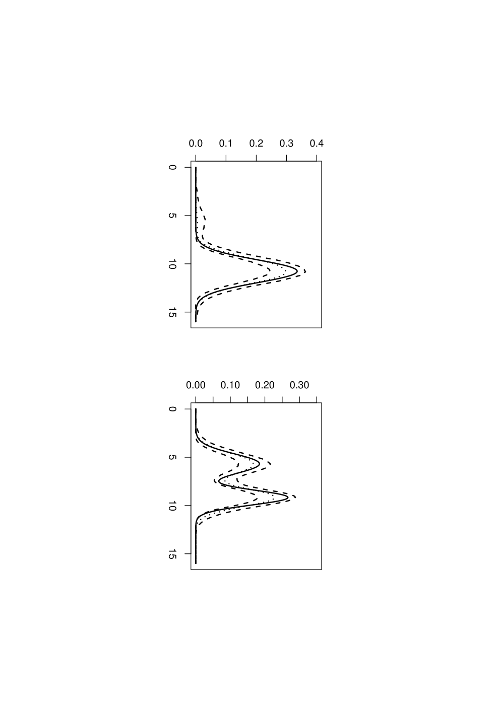
For every simulated data above, we apply the algorithm in Section 5 to obtain f^1\widehat{f}_{1} and f^2\widehat{f}_{2}. The 5%, 50%, and 95% point-wise quantiles for f^1\widehat{f}_{1} (left panel) and f^2\widehat{f}_{2} (right panel) over 1000 replications are given in Figure 1 (Study I: top panels; Study II: middle panels). We notice that the 90% confidence bands of f1f_{1} and f2f_{2} cover the corresponding true density. To compare with the methods proposed by Ma et al. (2011), we compute the average values of integrated squared error (ISE) for f^1\widehat{f}_{1} and f^2\widehat{f}_{2} over 1000 replications in Studies I and II. The results together with those presented by Ma et al. (2011) are displayed in Table 1. For presentational brevity, in Table 1, we have only listed two proposed methods (namely “OLS, ICV” and “OLS, plug-in”) in that paper, since for other methods the displayed results are very similar or even worse than these. Here ISE is defined to be

I​S​E​(f^j)=∫{f^j​(x)−f0,j​(x)}2​𝑑x.\displaystyle ISE(\widehat{f}_{j})=\int\{\widehat{f}_{j}(x)-f_{0,j}(x)\}^{2}dx.

Overview Table 1, we have clearly observed that for Studies I and II, our method leads to smaller ISE values than methods proposed by Ma et al. (2011). The improvement is significant, particularly for the case that f0,1f_{0,1} and f0,2f_{0,2} are simulated similarly (i.e., Study I).

Table 1: Average values of the integrated square error (ISE) for the proposed method and Ma et al. (2011)’s method in combination with ICV and adapted plug-in method under Studies I and II. Each value in the table was computed from 1000 replications and is 100 ×\times the actual value.
Study I, n=400n=400 Study II, n=400n=400
Methods f1f_{1} f2f_{2} f1f_{1} f2f_{2}
Ma et al. (2011): OLS, ICV 0.73 0.73 0.19 0.07
Ma et al. (2011): OLS, plug-in 0.82 0.83 0.21 0.08
Our method 0.52 0.51 0.15 0.07

In the third study (Study III), we simulate densities that mimic the shape of those estimated from the real data example in Section 7. The data are generated by:

Xi|αi∼f2​(x)\displaystyle X_{i}|\alpha_{i}\sim f_{2}(x)\quad when i>n1\displaystyle i>n_{1}
Xi|αi∼0.677​f1​(x)+0.323​f2​(x)\displaystyle X_{i}|\alpha_{i}\sim 0.677f_{1}(x)+0.323f_{2}(x)\quad when i≤n1,\displaystyle i\leq n_{1},

where n1=211n_{1}=211, n2=81n_{2}=81, f1​(x)f_{1}(x), and f2​(x)f_{2}(x) are the pdfs of N⁡(10.77,1.19)N(10.77,1.19) and 0.48​N​(5.68,1.04)+0.52​N​(9.17,0.78)0.48N(5.68,1.04)+0.52N(9.17,0.78) respectively. Here, N⁡(μ,σ)N(\mu,\sigma) denotes normal distribution with mean μ\mu and variance σ2\sigma^{2}. We choose these f1​(x)f_{1}(x) and f2​(x)f_{2}(x) so that they have similar shapes as those estimated from the real data example in Section 7. We repeat the simulation 1000 times and therefore obtain 1000 replicated simulation data sets {Xi,𝜶i}i=1292\{X_{i},\mbox{\boldmath$\alpha$}_{i}\}_{i=1}^{292}.

For each simulated data presented above, a simple method to estimate f1​(x)f_{1}(x) and f2​(x)f_{2}(x) is as follows. Let f~2​(x)\widetilde{f}_{2}(x) be the kernel density estimate of f2​(x)f_{2}(x) based on Xn1+1,…,XnX_{n_{1}+1},\ldots,X_{n} and r~​(x)\widetilde{r}(x) be that of 0.677​f1​(x)+0.323​f2​(x)0.677f_{1}(x)+0.323f_{2}(x) based on X1,…,Xn1X_{1},\ldots,X_{n_{1}}. We then estimate f1​(x)f_{1}(x) by

f~1​(x)=r~​(x)−0.323​f~2​(x)0.677.\widetilde{f}_{1}(x)=\frac{\widetilde{r}(x)-0.323\widetilde{f}_{2}(x)}{0.677}.

This method is introduced in the introduction section of Ma et al. (2011). Obviously, f~1​(x)\widetilde{f}_{1}(x) is not necessarily to be nonnegative.

We compare the results by our method with those by the simple method above. When implementing the simple method, we use the quartic kernel and R function dpik() to obtain the bandwidths for f~2​(x)\widetilde{f}_{2}(x) and r~​(x)\widetilde{r}(x). The average ISEs over 1000 replications for f^1\widehat{f}_{1} and f^2\widehat{f}_{2} are both about 0.66×10−20.66\times 10^{-2}. In contrast, those for f~1\widetilde{f}_{1} and f~2\widetilde{f}_{2} are 0.68×10−20.68\times 10^{-2} and 0.87×10−20.87\times 10^{-2} respectively. These observations are not surprising. Appropriately accounting for the information carried by X1,…,Xn1X_{1},\ldots,X_{n_{1}}, which is not used by f~2\widetilde{f}_{2}, our method decreases the ISE of the estimate of f2​(x)f_{2}(x) by about 24%. In contrast, f~1\widetilde{f}_{1} has fully used the information carried in Xn1+1,…,XnX_{n_{1}+1},\ldots,X_{n}; without extra information on f1​(x)f_{1}(x), our method does not significantly outperform the simple method. However, f^1​(x)\widehat{f}_{1}(x) is guaranteed to be nonnegative, but f~1​(x)\widetilde{f}_{1}(x) is not. We have displayed in the bottom panel of Figure 1 the 5%, 50%, and 95% point-wise quantiles for f^1\widehat{f}_{1} (left panel) and f^2\widehat{f}_{2} (right panel) over 1000 replications. We have observed that the 90% confidence bands of f1f_{1} and f2f_{2} capture the corresponding true densities.

Figure 1: Pointwise quantile density estimates for Studies I (top panels), II (middle panels), and III (bottom panels). In each plot, the solid line is the true density and the other three curves are the pointwise quantiles for density estimates over 1000 replicates: median (dotted), 5% (dashed), and 95% (dashed).

Refer to caption

Refer to caption

Refer to caption

In addition, we are not able to compare the results of our method with those by Ma et al. (2011) as the corresponding implemented algorithm is not publicly available yet. However, we observe that in this specific example the method by that paper leads to similar density estimates as the simple method. In particular, with straightforward mathematical manipulations, one can show that the estimate of f2​(x)f_{2}(x) by that method is exactly the same as that by the simple method, whereas the estimate of f1​(x)f_{1}(x) is given by

f~1′​(x)=r~​(x)−0.323​f~2′​(x)0.677,\displaystyle\widetilde{f}_{1}^{\prime}(x)=\frac{\widetilde{r}(x)-0.323\widetilde{f}_{2}^{\prime}(x)}{0.677},

with f~2​(x)\widetilde{f}_{2}(x) being the kernel density based on Xn1+1,…,XnX_{n_{1}+1},\ldots,X_{n}, but using the same bandwidth as r~​(x)\widetilde{r}(x); in contrast, the corresponding term in the simple method is f~2​(x)\widetilde{f}_{2}(x) whose bandwidth is chosen based on Xn1+1,…,XnX_{n_{1}+1},\ldots,X_{n}.

7 Real Data Example

We consider the malaria data described by Vounatsou et al. (1998). The data come from a cross-sectional survey of parasitemia and fever of children less than a year old in a village in the Kilombero district of Tanzania (Kitua et al. 1996). They considered a subset of this data for children of between six and nine months collected in two seasons: (1) January–June, the wet season, when malaria prevalence is high; (2) July–December, the dry season, when malaria prevalence is low. The data sets are available from http://www.blackwellpublishers.
co.uk/rss
. We use one of these data sets, which has also been analyzed by Qin and Leung (2005) and Yu et al. (2014) with other statistical methods.

The measurements are the parasite levels (per μ​l\mu l), ranging from 0 to 399952.1399952.1. Among these measurements, there are n1=211n_{1}=211 observations with positive parasite levels from the mixture sample and n2=81n_{2}=81 observations with positive parasite levels for nonmalaria cases in the community. Therefore, if we denote these parasite levels (after log transformation) as X1,…,Xn1,Xn1+1,…,XnX_{1},\ldots,X_{n_{1}},X_{n_{1}+1},\dots,X_{n} with n=n1+n2n=n_{1}+n_{2}, then

Xi|αi∼αi​f1​(x)+(1−αi)​f2​(x),\displaystyle X_{i}|\alpha_{i}\sim\alpha_{i}f_{1}(x)+(1-\alpha_{i})f_{2}(x),

where f1​(x)f_{1}(x) and f2​(x)f_{2}(x) are the pdfs of the log parasite levels for the malaria and nonmalaria subjects respectively; αi\alpha_{i} is the probability that the iith subject is a malaria patient. Clearly, when i>n1i>n_{1}, αi=0\alpha_{i}=0 as it is known that all the subjects in this group are nonmalaria patients. When i≤n1i\leq n_{1}, αi≈0.677\alpha_{i}\approx 0.677 estimated from the proportional of the malaria patients over the fevered patients in the endemicity and the community (Qin and Leung 2005). Therefore,

Xi|αi∼f2​(x)\displaystyle X_{i}|\alpha_{i}\sim f_{2}(x)\quad when i>n1\displaystyle i>n_{1}
Xi|αi∼0.677​f1​(x)+0.323​f2​(x)\displaystyle X_{i}|\alpha_{i}\sim 0.677f_{1}(x)+0.323f_{2}(x)\quad when i≤n1.\displaystyle i\leq n_{1}.

We apply our method and the simple method described in Section 6 on {Xi,𝜶i}i=1n\{X_{i},\mbox{\boldmath$\alpha$}_{i}\}_{i=1}^{n} above, where 𝜶i=(αi,1−αi)τ\mbox{\boldmath$\alpha$}_{i}=(\alpha_{i},1-\alpha_{i})^{\tau}. Bandwidths are selected by the algorithm in Section 5, and we get h1=0.832h_{1}=0.832 and h2=1.127h_{2}=1.127. The resultant density estimates f^1​(x)\widehat{f}_{1}(x), f^2​(x)\widehat{f}_{2}(x), f~1​(x)\widetilde{f}_{1}(x), and f~2​(x)\widetilde{f}_{2}(x) are diplayed in Figure 2. Both the “hat” and “tilde” estimates for f1f_{1} (and f2f_{2}) are similar in shape. But f~1​(x)\widetilde{f}_{1}(x) is not always nonnegative. Together with the observations in our simulation studies, we expect that f^1​(x)\widehat{f}_{1}(x) and f^2​(x)\widehat{f}_{2}(x) are more efficient than f~1​(x)\widetilde{f}_{1}(x) and f~2​(x)\widetilde{f}_{2}(x). We have also displayed the histograms for the nonmalaria sample [i.e., that for f2​(x)f_{2}(x)] and the mixture sample [i.e., that for 0.677​f1​(x)+0.323​f2​(x)0.677f_{1}(x)+0.323f_{2}(x)] with the corresponding density estimates from our method in Figure 3. From this figure, we observe that our density estimates agree very well with the observed data (see the histogram of the observations from the respective sample).

Figure 2: Component density estimates for malaria data based on the proposed method and the simple method described in Section 6.

Refer to caption

Figure 3: Histograms for the nonmalaria sample [i.e., that for f2​(x)f_{2}(x)] and the mixture sample [i.e., that for 0.677​f1​(x)+0.323​f2​(x)0.677f_{1}(x)+0.323f_{2}(x)] along with the corresponding density estimates based on the proposed method.

Refer to caption

Furthermore, from Figure 2, we observe that the density estimate for the log parasite levels of the malaria patients (the black solid line) has a clearer peak and more concentrated curve (centered around 11) than that for the nonmalaria sample (the red dashed line), which has a bimodal feature. From practical point of view, we argue that such an observation is not surprising: the log parasite levels for the nonmalaria sample may be resulted from more than one cause; these causes may lead to different parasite levels and therefore the corresponding density is in fact a mixture of a number of subpopulations. In contrast, the cause for the malaria sample is clear, i.e., the malaria disease; therefore, the resultant density is concentrated and has a clear peak.

Appendix A: Proof of Theorems 1–3

Proof of Theorem 1

The proof of this theorem uses a similar strategy as that in Levine et. al. (2011). Recall that for (f1,…,fM)∈𝒞(f_{1},\ldots,f_{M})\in\mathcal{C}, wi,j=αi,j​𝒩hj​fj​(Xi)∑k=1Mαi,k​𝒩hk​fk​(Xi)w_{i,j}=\frac{\alpha_{i,j}\mbox{$\mathcal{N}$}_{h_{j}}f_{j}(X_{i})}{\sum_{k=1}^{M}\alpha_{i,k}\mbox{$\mathcal{N}$}_{h_{k}}f_{k}(X_{i})}. Then for every i=1,…,ni=1,\ldots,n, ∑j=1Mwi,j\sum_{j=1}^{M}w_{i,j} = 1. By the concavity of the logarithm function, we have for every (g1,…,gM)∈𝒞(g_{1},\ldots,g_{M})\in\mathcal{C},

ln​(g1,…,gM)−ln​(f1,…,fM)\displaystyle l_{n}(g_{1},\ldots,g_{M})-l_{n}(f_{1},\ldots,f_{M}) (A.1)
=\displaystyle= ∑i=1nlog⁡∑j=1Mαi​j​𝒩hj​gj​(Xi)∑j=1Mαi​j​𝒩hj​fj​(Xi)\displaystyle\sum_{i=1}^{n}\log\frac{\sum_{j=1}^{M}\alpha_{ij}\mbox{$\mathcal{N}$}_{h_{j}}g_{j}(X_{i})}{\sum_{j=1}^{M}\alpha_{ij}\mbox{$\mathcal{N}$}_{h_{j}}f_{j}(X_{i})}
=\displaystyle= ∑i=1nlog∑j=1Mwi,j𝒩hj​gj​(Xi)𝒩hj​fj​(Xi)\displaystyle\sum_{i=1}^{n}\log\sum_{j=1}^{M}w_{i,j}\frac{\mbox{$\mathcal{N}$}_{h_{j}}g_{j}(X_{i})}{\mbox{$\mathcal{N}$}_{h_{j}}f_{j}(X_{i})}
≥\displaystyle\geq ∑i=1n∑j=1Mwi,j​{log⁡𝒩hj​gj​(Xi)−log⁡𝒩hj​fj​(Xi)}\displaystyle\sum_{i=1}^{n}\sum_{j=1}^{M}w_{i,j}\left\{\log\mbox{$\mathcal{N}$}_{h_{j}}g_{j}(X_{i})-\log\mbox{$\mathcal{N}$}_{h_{j}}f_{j}(X_{i})\right\}
=\displaystyle= ∑j=1M{bj​(g1,…,gM)−bj​(f1,…,fM)},\displaystyle\sum_{j=1}^{M}\left\{b_{j}(g_{1},\ldots,g_{M})-b_{j}(f_{1},\ldots,f_{M})\right\},

where

bj​(g1,…,gM)\displaystyle b_{j}(g_{1},\ldots,g_{M}) =\displaystyle= ∑i=1nwi,j​log⁡𝒩hj​gj​(Xi)\displaystyle\sum_{i=1}^{n}w_{i,j}\log\mbox{$\mathcal{N}$}_{h_{j}}g_{j}(X_{i}) (A.2)
=\displaystyle= ∫∑i=1nwi,j​Kh​(u−Xi)​log⁡gj​(u)​𝑑u,\displaystyle\int\sum_{i=1}^{n}w_{i,j}K_{h}(u-X_{i})\log g_{j}(u)du,

which is maximized when gj​(x)=∑i=1nwi,j​Kh​(x−Xi)∑i=1nwi,j=fj𝒢​(x)g_{j}(x)=\frac{\sum_{i=1}^{n}w_{i,j}K_{h}(x-X_{i})}{\sum_{i=1}^{n}w_{i,j}}=f_{j}^{\mathcal{G}}(x). This together with (A.1) completes the proof of this theorem.  ■\blacksquare

Proof of Theorem 2

We first show necessity. Assume ln​(f^1,…,f^M)=sup(f1,…,fM)∈𝒞ln​(f1,…,fM)l_{n}(\widehat{f}_{1},\ldots,\widehat{f}_{M})=\sup_{(f_{1},\ldots,f_{M})\in\mathcal{C}}l_{n}(f_{1},\ldots,f_{M}). Based on Theorem 1, we immediately have l⁡(f^1,…,f^M)=l⁡(𝒢⁡(f^1,…,f^M))l(\widehat{f}_{1},\ldots,\widehat{f}_{M})=l(\mathcal{G}(\widehat{f}_{1},\ldots,\widehat{f}_{M})). Next we show that (f^1,…,f^M)=𝒢⁡(f^1,…,f^M)(\widehat{f}_{1},\ldots,\widehat{f}_{M})=\mathcal{G}(\widehat{f}_{1},\ldots,\widehat{f}_{M}).

With exactly the same calculation as (A.1) and (A.2), we have

0\displaystyle 0 =\displaystyle= l⁡(𝒢⁡(f^1,…,f^M))−l⁡(f^1,…,f^M)\displaystyle l(\mathcal{G}(\widehat{f}_{1},\ldots,\widehat{f}_{M}))-l(\widehat{f}_{1},\ldots,\widehat{f}_{M})
≥\displaystyle\geq ∑j=1M{(∑i=1nw^i,j)​∫f^j𝒢​(x)​log⁡f^j𝒢​(x)f^j​(x)​𝑑x},\displaystyle\sum_{j=1}^{M}\left\{\left(\sum_{i=1}^{n}\widehat{w}_{i,j}\right)\int\widehat{f}_{j}^{\mathcal{G}}(x)\log\frac{\widehat{f}_{j}^{\mathcal{G}}(x)}{\widehat{f}_{j}(x)}dx\right\},

where f^j𝒢\widehat{f}_{j}^{\mathcal{G}} denotes the jjth component of 𝒢⁡(f^1,…,f^M)\mathcal{G}(\widehat{f}_{1},\ldots,\widehat{f}_{M}), w^i,j=αi,j​𝒩hj​f^j​(Xi)∑k=1Mαi,k​𝒩hk​f^k​(Xi)\widehat{w}_{i,j}=\frac{\alpha_{i,j}\mbox{$\mathcal{N}$}_{h_{j}}\widehat{f}_{j}(X_{i})}{\sum_{k=1}^{M}\alpha_{i,k}\mbox{$\mathcal{N}$}_{h_{k}}\widehat{f}_{k}(X_{i})}. On the other hand, as f^j𝒢\widehat{f}_{j}^{\mathcal{G}} and f^j\widehat{f}_{j} are pdfs, we have

∫f^j𝒢​(x)​log⁡f^j𝒢​(x)f^j​(x)​𝑑x≥0.\displaystyle\int\widehat{f}_{j}^{\mathcal{G}}(x)\log\frac{\widehat{f}_{j}^{\mathcal{G}}(x)}{\widehat{f}_{j}(x)}dx\geq 0.

Furthermore for every j=1,…,Mj=1,\ldots,M, since ∑i=1nαi,j>0\sum_{i=1}^{n}\alpha_{i,j}>0 and (f^1,…,f^M)∈𝒞(\widehat{f}_{1},\ldots,\widehat{f}_{M})\in\mathcal{C}, we have ∑i=1nw^i,j>0\sum_{i=1}^{n}\widehat{w}_{i,j}>0. Therefore,

∫f^j𝒢​(x)​log⁡f^j𝒢​(x)f^j​(x)​𝑑x=0,\displaystyle\int\widehat{f}_{j}^{\mathcal{G}}(x)\log\frac{\widehat{f}_{j}^{\mathcal{G}}(x)}{\widehat{f}_{j}(x)}dx=0,

which together with the continuity of f^j​(x)\widehat{f}_{j}(x) and f^j𝒢​(x)\widehat{f}_{j}^{\mathcal{G}}(x), and the fact that log⁡(⋅)\log(\cdot) is strictly concave leads to f^j𝒢​(x)=f^j​(x)\widehat{f}_{j}^{\mathcal{G}}(x)=\widehat{f}_{j}(x) for every x∈Sxx\in S_{x}. That is (f^1,…,f^M)=𝒢⁡(f^1,…,f^M)(\widehat{f}_{1},\ldots,\widehat{f}_{M})=\mathcal{G}(\widehat{f}_{1},\ldots,\widehat{f}_{M}) as claimed before.

We proceed to show the sufficiency. Assume (f^1,…,f^M)=𝒢⁡(f^1,…,f^M)(\widehat{f}_{1},\ldots,\widehat{f}_{M})=\mathcal{G}(\widehat{f}_{1},\ldots,\widehat{f}_{M}). Let 𝒇^=(f^1,…,f^M)\widehat{\boldsymbol{f}}=(\widehat{f}_{1},\ldots,\widehat{f}_{M}). For an arbitrary 𝒇=(f1,…,fM)∈ℱn{\boldsymbol{f}}=(f_{1},\ldots,f_{M})\in\mathcal{F}_{n}, we need to show that ln​(𝒇)≤ln​(𝒇^)l_{n}({\boldsymbol{f}})\leq l_{n}(\widehat{\boldsymbol{f}}).

Define

H⁡(t)=ln​(𝒇^+t⁡(𝒇−𝒇^)),\displaystyle H(t)=l_{n}(\widehat{\boldsymbol{f}}+t({\boldsymbol{f}}-\widehat{\boldsymbol{f}})), (A.3)

with t∈[0,1]t\in[0,1]. Next, we verify that H⁡(⋅)H(\cdot) has the following properties.

  • (P1).

    H⁡(t)H(t) is a concave function in [0,1][0,1].

  • (P2).

    H⁡(t)H(t) is continuously differentiable in (0,1)(0,1), H′​(0+)H^{\prime}(0+) exists, and H′​(0+)=0H^{\prime}(0+)=0.

We first show (P1) above. Note that lnl_{n} is concave in 𝒞\mathcal{C}, we immediately have for every t1,t2∈[0,1]t_{1},t_{2}\in[0,1],

H⁡(t1+t22)\displaystyle H\left(\frac{t_{1}+t_{2}}{2}\right) =\displaystyle= ln​({𝒇^+t1​(𝒇−𝒇^)}+{𝒇^+t2​(𝒇−𝒇^)}2)\displaystyle l_{n}\left(\frac{\left\{\widehat{\boldsymbol{f}}+t_{1}({\boldsymbol{f}}-\widehat{\boldsymbol{f}})\right\}+\left\{\widehat{\boldsymbol{f}}+t_{2}({\boldsymbol{f}}-\widehat{\boldsymbol{f}})\right\}}{2}\right)
≥\displaystyle\geq 12​ln​(𝒇^+t1​(𝒇−𝒇^))+12​ln​(𝒇^+t2​(𝒇−𝒇^))\displaystyle\frac{1}{2}l_{n}\left(\widehat{\boldsymbol{f}}+t_{1}({\boldsymbol{f}}-\widehat{\boldsymbol{f}})\right)+\frac{1}{2}l_{n}\left(\widehat{\boldsymbol{f}}+t_{2}({\boldsymbol{f}}-\widehat{\boldsymbol{f}})\right)
=\displaystyle= 12​H​(t1)+12​H​(t2),\displaystyle\frac{1}{2}H(t_{1})+\frac{1}{2}H(t_{2}),

leading to (P1). We proceed to show (P2). First, to verify that H⁡(t)H(t) is continuously differentiable in (0,1)(0,1) and the existence of H′​(0+)H^{\prime}(0+), it suffices to verify that for every x∈Sxx\in S_{x} and j=1,…,Mj=1,\ldots,M, ∫Kh​(u−x)​log⁡[f^j​(u)+t⁡{fj​(u)−f^j​(u)}]​𝑑u\int K_{h}(u-x)\log\left[\widehat{f}_{j}(u)+t\left\{f_{j}(u)-\widehat{f}_{j}(u)\right\}\right]du is continuously differentiable when t∈(0,1)t\in(0,1), right differentiable at t=0t=0, and the derivative can be exchanged with the integration. This is valid because of the definition of ℱn\mathcal{F}_{n} and the dominant convergence theorem. Therefore, it is left to verify H′​(0+)=0H^{\prime}(0+)=0. For notational convenience, we denote 𝒇t=𝒇^+t⁡(𝒇−𝒇^)=(f1,t,…,fM,t){\boldsymbol{f}}_{t}=\widehat{\boldsymbol{f}}+t({\boldsymbol{f}}-\widehat{\boldsymbol{f}})=(f_{1,t},\ldots,f_{M,t}) and let (f1,t𝒢,…,fM,t𝒢)=𝒢⁡(f1,t,…,fM,t)(f_{1,t}^{\mathcal{G}},\ldots,f_{M,t}^{\mathcal{G}})=\mathcal{G}(f_{1,t},\ldots,f_{M,t}). Using the chain rule of derivatives, we have for every t∈(0,1)t\in(0,1),

H′​(t)\displaystyle H^{\prime}(t) =\displaystyle= ∑i=1n∑j=1Mαi,j​𝒩hj​fj,t∑k=1Mαi,k​𝒩hk​fk,t​(Xi)​∫Khj​(u−Xi)fj,t​(u)​{fj​(u)−f^j​(u)}​𝑑u\displaystyle\sum_{i=1}^{n}\sum_{j=1}^{M}\frac{\alpha_{i,j}\mbox{$\mathcal{N}$}_{h_{j}}f_{j,t}}{\sum_{k=1}^{M}\alpha_{i,k}\mbox{$\mathcal{N}$}_{h_{k}}f_{k,t}(X_{i})}\int\frac{K_{h_{j}}(u-X_{i})}{f_{j,t}(u)}\left\{f_{j}(u)-\widehat{f}_{j}(u)\right\}du
=\displaystyle= ∑j=1M∫fj,t𝒢​(u)fj,t​(u)​{fj​(u)−f^j​(u)}​𝑑u.\displaystyle\sum_{j=1}^{M}\int\frac{f_{j,t}^{\mathcal{G}}(u)}{f_{j,t}(u)}\left\{f_{j}(u)-\widehat{f}_{j}(u)\right\}du.

Noting the fact that fj,0=f^jf_{j,0}=\widehat{f}_{j} and f^j𝒢=f^j\widehat{f}_{j}^{\mathcal{G}}=\widehat{f}_{j} based on our assumption, we immediately have

H′​(0+)\displaystyle H^{\prime}(0+) =\displaystyle= ∑j=1M∫fj,0𝒢​(u)fj,0​(u)​{fj​(u)−f^j​(u)}​𝑑u\displaystyle\sum_{j=1}^{M}\int\frac{f_{j,0}^{\mathcal{G}}(u)}{f_{j,0}(u)}\left\{f_{j}(u)-\widehat{f}_{j}(u)\right\}du
=\displaystyle= ∑j=1M∫{fj​(u)−f^j​(u)}​𝑑u=0,\displaystyle\sum_{j=1}^{M}\int\left\{f_{j}(u)-\widehat{f}_{j}(u)\right\}du=0,

which completes our proof of (P2) above. Now based on (P1) and (P2) and the property of the concave functions, we immediately have

H⁡(1)≤H⁡(0)+H′​(0+)​(1−0),\displaystyle H(1)\leq H(0)+H^{\prime}(0+)(1-0),

which is

ln​(𝒇)≤ln​(𝒇^).\displaystyle l_{n}({\boldsymbol{f}})\leq l_{n}(\widehat{\boldsymbol{f}}).

This completes the proof of the theorem.  ■\blacksquare

Proof of Theorem 3

Since (f1s,…,fMs)∈ℱn(f_{1}^{s},\ldots,f_{M}^{s})\in\mathcal{F}_{n}, for every j=1,…,Mj=1,\ldots,M, we can write

fjs​(x)=∑i=1nwi,js​Khj​(x−Xi)∑i=1nwi,js.\displaystyle f_{j}^{s}(x)=\frac{\sum_{i=1}^{n}w_{i,j}^{s}K_{h_{j}}(x-X_{i})}{\sum_{i=1}^{n}w_{i,j}^{s}}.

Clearly, for every ss, the collection of the coefficients ws={wi,js:i=1,…,n;j=1,…,M}w^{s}=\{w_{i,j}^{s}:i=1,\ldots,n;j=1,\ldots,M\} belongs to

Ωw={{wi,j:i=1,…,n;j=1,…,M}:0≤wi,j≤1},\displaystyle\Omega_{w}=\left\{\{w_{i,j}:i=1,\ldots,n;j=1,\ldots,M\}:0\leq w_{i,j}\leq 1\right\},

which is a closed subset of ℝn​M\mathbb{R}^{nM}. Therefore, there exists a subsequence of wsw^{s}, namely wslw^{s_{l}}, and w∞={wi,j∞:i=1,…,n;j=1,…,M}∈Ωww^{\infty}=\{w_{i,j}^{\infty}:i=1,\ldots,n;j=1,\ldots,M\}\in\Omega_{w}, such that

liml→∞wsl=w∞.\displaystyle\lim_{l\to\infty}w^{s_{l}}=w^{\infty}. (A.4)

Let

fj∞​(x)=∑i=1nwi,j∞​Khj​(x−Xi)∑i=1nwi,j∞.\displaystyle f_{j}^{\infty}(x)=\frac{\sum_{i=1}^{n}w_{i,j}^{\infty}K_{h_{j}}(x-X_{i})}{\sum_{i=1}^{n}w_{i,j}^{\infty}}.

It can be readily checked that

liml→∞fjsl​(x)=fj∞​(x)\lim_{l\to\infty}f_{j}^{s_{l}}(x)=f_{j}^{\infty}(x) (A.5)

for all x∈Sxx\in S_{x} and hence

liml→∞ln​(f1sl,…,fMsl)=ln​(f1∞,…,fM∞),\displaystyle\lim_{l\to\infty}l_{n}(f_{1}^{s_{l}},\ldots,f_{M}^{s_{l}})=l_{n}(f_{1}^{\infty},\ldots,f_{M}^{\infty}),

which together with Theorem 1 ensures

lims→∞ln​(f1s,…,fMs)=ln​(f1∞,…,fM∞).\displaystyle\lim_{s\to\infty}l_{n}(f_{1}^{s},\ldots,f_{M}^{s})=l_{n}(f_{1}^{\infty},\ldots,f_{M}^{\infty}).

It is left to show

𝒢⁡(f1∞,…,fM∞)=(f1∞,…,fM∞).\displaystyle\mathcal{G}(f_{1}^{\infty},\ldots,f_{M}^{\infty})=(f_{1}^{\infty},\ldots,f_{M}^{\infty}). (A.6)

Then based on Theorem 2, we have

ln​(f1∞,…,fM∞)=ln​(f^1,…,f^M),l_{n}(f_{1}^{\infty},\ldots,f_{M}^{\infty})=l_{n}(\widehat{f}_{1},\ldots,\widehat{f}_{M}),

which completes our proof of this theorem.

In fact, along the subsequence sls_{l} defined above, using the same derivations as (A.1) and (A.2), we have

0\displaystyle 0 =\displaystyle= liml→∞{ln​(f1sl+1,…,fMsl+1)−ln​(f1sl,…,fMsl)}\displaystyle\lim_{l\to\infty}\left\{l_{n}(f_{1}^{s_{l}+1},\ldots,f_{M}^{s_{l}+1})-l_{n}(f_{1}^{s_{l}},\ldots,f_{M}^{s_{l}})\right\}
≥\displaystyle\geq liml→∞∑j=1M{(∑i=1nwi,jsl)​∫fjsl+1​(x)​log⁡fjsl+1​(x)fjsl​(x)​𝑑x}≥0.\displaystyle\lim_{l\to\infty}\sum_{j=1}^{M}\left\{\left(\sum_{i=1}^{n}w_{i,j}^{s_{l}}\right)\int f_{j}^{s_{l}+1}(x)\log\frac{f_{j}^{s_{l}+1}(x)}{f_{j}^{s_{l}}(x)}dx\right\}\geq 0.

Hence

liml→∞∑j=1M{(∑i=1nwi,jsl)​∫fjsl+1​(x)​log⁡fjsl+1​(x)fjsl​(x)​𝑑x}=0.\lim_{l\to\infty}\sum_{j=1}^{M}\left\{\left(\sum_{i=1}^{n}w_{i,j}^{s_{l}}\right)\int f_{j}^{s_{l}+1}(x)\log\frac{f_{j}^{s_{l}+1}(x)}{f_{j}^{s_{l}}(x)}dx\right\}=0. (A.7)

On the other hand, note that (A.5) implies liml→∞𝒢⁡(f1sl,…,fMsl)=𝒢⁡(f1∞,…,fM∞)\lim_{l\to\infty}\mathcal{G}(f_{1}^{s_{l}},\ldots,f_{M}^{s_{l}})=\mathcal{G}(f_{1}^{\infty},\ldots,f_{M}^{\infty}), or equivalently,

liml→∞(f1sl+1,…,fMsl+1)=(f1∞,𝒢,…,fM∞,𝒢),\lim_{l\to\infty}(f_{1}^{s_{l}+1},\ldots,f_{M}^{s_{l}+1})=(f_{1}^{\infty,\mathcal{G}},\ldots,f_{M}^{\infty,\mathcal{G}}), (A.8)

where (f1∞,𝒢,…,fM∞,𝒢)=𝒢⁡(f1∞,…,fM∞)(f_{1}^{\infty,\mathcal{G}},\ldots,f_{M}^{\infty,\mathcal{G}})=\mathcal{G}(f_{1}^{\infty},\ldots,f_{M}^{\infty}). Combining (A.4), (A.5), (A.7), and (A.8), we have

∑j=1M{(∑i=1nwi,j∞)​∫fj∞,𝒢​(x)​log⁡fj∞,𝒢​(x)fj∞​(x)​𝑑x}=0,\sum_{j=1}^{M}\left\{\left(\sum_{i=1}^{n}w_{i,j}^{\infty}\right)\int f_{j}^{\infty,\mathcal{G}}(x)\log\frac{f_{j}^{\infty,\mathcal{G}}(x)}{f_{j}^{\infty}(x)}dx\right\}=0,

which indicates for every j=1,…,Mj=1,\ldots,M,

∫fj∞,𝒢​(x)​log⁡fj∞,𝒢​(x)fj∞​(x)​𝑑x=0.\displaystyle\int f_{j}^{\infty,\mathcal{G}}(x)\log\frac{f_{j}^{\infty,\mathcal{G}}(x)}{f_{j}^{\infty}(x)}dx=0. (A.9)

With the continuity of fj∞​(x)f_{j}^{\infty}(x) and fj∞,𝒢​(x)f_{j}^{\infty,\mathcal{G}}(x), and the fact that log⁡(⋅)\log(\cdot) is strictly concave, (A.9) implies fj∞​(x)=fj∞,𝒢​(x)f_{j}^{\infty}(x)=f_{j}^{\infty,\mathcal{G}}(x). That is

𝒢⁡(f1∞,…,fM∞)=(f1∞,…,fM∞),\displaystyle\mathcal{G}(f_{1}^{\infty},\ldots,f_{M}^{\infty})=(f_{1}^{\infty},\ldots,f_{M}^{\infty}),

which proves (A.6), and therefore completes the proof of this theorem.  ■\blacksquare

Appendix B: Proof of Theorems 4 – 6

Technical Conditions

We impose the following conditions to facilitate our technical developments for Theorems 5 and 6. They are not necessarily the weakest possible.

  • Condition 1: There exists a bandwidth hh such that C1≤infn,jhj/h≤supn,jhj/h≤C2C_{1}\leq\inf_{n,j}h_{j}/h\leq\sup_{n,j}h_{j}/h\leq C_{2}, where C1>0C_{1}>0 and C2>0C_{2}>0 are universal constants. Furthermore, h→0h\to 0 and n​h→∞nh\to\infty when n→∞n\to\infty.

  • Condition 2: The kernel function K⁡(x)K(x) is symmetric about 0, supported and continuous on [−L,L][-L,L] for some L>0L>0 and infx∈[−L,L]K⁡(x)>0\inf_{x\in[-L,L]}K(x)>0. The aath-order derivative K(a)​(x)K^{(a)}(x) of K⁡(x)K(x) exists for every a=1,2,…a=1,2,\ldots and x∈(−L,L)x\in(-L,L). Further supa,x|K(a)​(x)|\sup_{a,x}|K^{(a)}(x)| is bounded.

  • Condition 3: The true component pdfs f0,j​(x)f_{0,j}(x), j=1,…,Mj=1,\ldots,M are supported on Sx=[c1,c2]S_{x}=[c_{1},c_{2}] and are twice continuously differentiable in (c1,c2)(c_{1},c_{2}) with bounded second order derivatives. Furthermore, infx∈Sxf0,j​(x)>0\inf_{x\in S_{x}}f_{0,j}(x)>0.

  • Condition 4: Let SγS_{\gamma} be the support for γ⁡(𝜶)\gamma(\mbox{\boldmath$\alpha$}). There exists M×1M\times 1 vectors 𝜶0,1,…,𝜶0,M\mbox{\boldmath$\alpha$}_{0,1},\ldots,\mbox{\boldmath$\alpha$}_{0,M} in SγS_{\gamma} satisfy (i) and (ii) below.

    • (i).

      The MM vectors 𝜶0,1,…,𝜶0,M\mbox{\boldmath$\alpha$}_{0,1},\ldots,\mbox{\boldmath$\alpha$}_{0,M} are linearly independent.

    • (ii).

      There exist balls 𝒪j⊂Sγ,j=1,…,M\mathcal{O}_{j}\subset S_{\gamma},j=1,\ldots,M, 𝜶0,j∈𝒪j\mbox{\boldmath$\alpha$}_{0,j}\in\mathcal{O}_{j}, 𝒪j\mathcal{O}_{j} are disjoint, and γ⁡(𝜶)>0\gamma(\mbox{\boldmath$\alpha$})>0 for every 𝜶∈𝒪j\mbox{\boldmath$\alpha$}\in\mathcal{O}_{j}.

    Condition 1 requires that the MM bandwidths have the same order. Condition 2 requires that the kernel function K⁡(x)K(x) is symmetric and is sufficiently smooth. Condition 3 requires the component pdfs are sufficiently smooth and is positive on the support of XX. Condition 4 is a identifiability condition, which is satisfied when 𝜶\alpha is a continuous random vector, or a discrete random vector with at least MM supports.

Preliminary preparation

The proof of Theorems 4–6 heavily relies on the well developed results for the M-estimation in empirical process. We use van der Vaart and Wellner (1996) (VM) as the main reference and adapt the commonly used notation in this book. In this section, we introduce some necessary notation and review two important results.

We first review some notation necessary for introducing the result for the M-estimation. Let `​`≲"``\lesssim" (`​`≳"``\gtrsim") denote smaller (greater) than, up to a universal constant. Throughout, we will use CC to denote a sufficiently large universal constant. For a set ℳ\mathcal{M} of functions of (x,𝜶)(x,\mbox{\boldmath$\alpha$}), we define

𝔾n​m\displaystyle\mathbb{G}_{n}m =\displaystyle= n​{1n​∑i=1nm⁡(Xi,𝜶i)−E0​m​(X,𝜶)}​ for ​m∈ℳ\displaystyle\sqrt{n}\left\{\frac{1}{n}\sum_{i=1}^{n}m(X_{i},\mbox{\boldmath$\alpha$}_{i})-E_{0}m(X,\mbox{\boldmath$\alpha$})\right\}\mbox{ for }m\in\mathcal{M} (B.1)
‖𝔾n‖ℳ\displaystyle||\mathbb{G}_{n}||_{\mathcal{M}} =\displaystyle= supm∈ℳ|𝔾n​m|.\displaystyle\sup_{m\in\mathcal{M}}\left|\mathbb{G}_{n}m\right|. (B.2)

Here E0E_{0} means the expectation is taken under γ⁡(𝜶)​p~0​(x,𝜶)\gamma(\mbox{\boldmath$\alpha$})\widetilde{p}_{0}(x,\mbox{\boldmath$\alpha$}). This convention will be used throughout the proof. The Hellinger distance between two non-negative functions m1​(x,𝜶)m_{1}(x,\mbox{\boldmath$\alpha$}) and m2​(x,𝜶)m_{2}(x,\mbox{\boldmath$\alpha$}) is defined to be

d⁡(m1,m2)=[∫Sγ∫ℝ{m11/2​(x,𝜶)−m21/2​(x,𝜶)}2​𝑑x​𝑑𝜶]1/2.\displaystyle d(m_{1},m_{2})=\left[\int_{S_{\gamma}}\int_{\mathbb{R}}\left\{m_{1}^{1/2}(x,\mbox{\boldmath$\alpha$})-m_{2}^{1/2}(x,\mbox{\boldmath$\alpha$})\right\}^{2}dxd\mbox{\boldmath$\alpha$}\right]^{1/2}.

Let 𝒫n\mathcal{P}_{n} denote the class of functions:

𝒫n\displaystyle\mathcal{P}_{n} =\displaystyle= {p⁡(x,𝜶)=∑j=1Mαj​𝒩hj​fj​(x):(f1,…,fM)∈ℱn},\displaystyle\left\{p(x,\mbox{\boldmath$\alpha$})=\sum_{j=1}^{M}\alpha_{j}\mbox{$\mathcal{N}$}_{h_{j}}f_{j}(x):(f_{1},\ldots,f_{M})\in\mathcal{F}_{n}\right\}, (B.3)

where ℱn\mathcal{F}_{n} is defined by (7). For any nonnegative functions p⁡(x,𝜶)p(x,\mbox{\boldmath$\alpha$}) and p1​(x,𝜶)p_{1}(x,\mbox{\boldmath$\alpha$}), we define

mp,p1​(X,𝜶)\displaystyle m_{p,p_{1}}(X,\mbox{\boldmath$\alpha$}) =\displaystyle= log⁡p⁡(X,𝜶)+p1​(X,𝜶)2​p1​(X,𝜶);\displaystyle\log\frac{p(X,\mbox{\boldmath$\alpha$})+p_{1}(X,\mbox{\boldmath$\alpha$})}{2p_{1}(X,\mbox{\boldmath$\alpha$})}; (B.4)
𝕄n​(p,p1)\displaystyle\mathbb{M}_{n}(p,p_{1}) =\displaystyle= 1n​∑i=1nmp,p1​(Xi,𝜶i);\displaystyle\frac{1}{n}\sum_{i=1}^{n}m_{p,p_{1}}(X_{i},\mbox{\boldmath$\alpha$}_{i}); (B.5)
Mn​(p,p1)\displaystyle M_{n}(p,p_{1}) =\displaystyle= E0​mp,p1​(X,𝜶);\displaystyle E_{0}m_{p,p_{1}}(X,\mbox{\boldmath$\alpha$}); (B.6)
ℳn,δ,p,p1\displaystyle\mathcal{M}_{n,\delta,p,p_{1}} =\displaystyle= {mp,p1−mp1,p1:p∈𝒫n,d(γp,γp1)<δ}.\displaystyle\left\{m_{p,p_{1}}-m_{p_{1},p_{1}}:p\in\mathcal{P}_{n},d(\gamma p,\gamma p_{1})<\delta\right\}. (B.7)

With the above preparation, we present an important lemma, which is an application of Theorem 3.4.1 of van der Vaart and Wellner (1996) to our current setup. It serves the basis for our subsequent proof.

Lemma 1.

Suppose the notation 𝕄n\mathbb{M}_{n}, MnM_{n}, and ‖𝔾n‖ℳn,δ,p,p~0\|\mathbb{G}_{n}\|_{\mathcal{M}_{n,\delta,p,\widetilde{p}_{0}}} are defined above, p~0​(x,𝛂)=∑j=1Mαj​f0,j​(x)\widetilde{p}_{0}(x,\mbox{\boldmath$\alpha$})=\sum_{j=1}^{M}\alpha_{j}f_{0,j}(x) is the true conditional density of XX given 𝛂\alpha, and γ⁡(⋅)\gamma(\cdot) is the marginal density of 𝛂\alpha. If the following three conditions are satisfied:

  1. (C1)

    for every nn and p∈ℱnp\in\mathcal{F}_{n}, Mn​(p,p~0)−Mn​(p~0,p~0)≲−d2​(γ​p,γ​p~0);M_{n}(p,\widetilde{p}_{0})-M_{n}(\widetilde{p}_{0},\widetilde{p}_{0})\lesssim-d^{2}(\gamma p,\gamma\widetilde{p}_{0});

  2. (C2)

    for every nn and δ>0\delta>0, E0​‖𝔾n‖ℳn,δ,p,p~0≲ϕn​(δ)E_{0}\|\mathbb{G}_{n}\|_{\mathcal{M}_{n,\delta,p,\widetilde{p}_{0}}}\lesssim\phi_{n}(\delta) for functions ϕn\phi_{n} such that ϕn​(δ)/δα\phi_{n}(\delta)/\delta^{\alpha} is decreasing on (0,∞)(0,\infty) for some α<2\alpha<2;

  3. (C3)

    𝕄n​(p^,p~0)≥𝕄n​(p~0,p~0)−Op​(rn−2)\mathbb{M}_{n}(\widehat{p},\widetilde{p}_{0})\geq\mathbb{M}_{n}(\widetilde{p}_{0},\widetilde{p}_{0})-O_{p}(r_{n}^{-2}), where p^​(x,𝜶)=∑j=1Mαj​𝒩hj​f^j​(x)\widehat{p}(x,\mbox{\boldmath$\alpha$})=\sum_{j=1}^{M}\alpha_{j}\mbox{$\mathcal{N}$}_{h_{j}}\widehat{f}_{j}(x) and rnr_{n} satisfies rn2​ϕ​(1/rn)≤n,r_{n}^{2}\phi(1/r_{n})\leq\sqrt{n}, for every nn;

then

rn​d​(γ​p^,γ​p~0)=Op​(1).r_{n}d(\gamma\widehat{p},\gamma\widetilde{p}_{0})=O_{p}(1).

An difficult step in the application of the above lemma is to verify Condition C2. An useful technique is to establish a connection between E0​‖𝔾n‖ℳn,δ,p,p~0E_{0}\|\mathbb{G}_{n}\|_{\mathcal{M}_{n,\delta,p,\widetilde{p}_{0}}} and the bracketing integral of the class γ​𝒫n\gamma\mathcal{P}_{n}. For the convenience of presentation in next subsections, we introduce some necessary notation and review an important lemma.

We first introduce the concept of bracketing numbers, which will be used to define the bracketing integral. Consider a set ℳ\mathcal{M} of functions and the norm ∥⋅∥\|\cdot\| defined on the set ℳ\mathcal{M}. For any ϵ>0\epsilon>0, the bracketing number N[](ϵ,ℳ,∥⋅∥)N_{[]}(\epsilon,\mathcal{M},\|\cdot\|) is the minimum number of NN for which there exists a set of pairs of functions {(lj,uj)}j=1N\{(l_{j},u_{j})\}_{j=1}^{N} such that (i) ‖uj−lj‖<ϵ\|u_{j}-l_{j}\|<\epsilon and (ii) for any m∈ℳm\in\mathcal{M}, there exists a j=j⁡(m)j=j(m) such that lj≤m≤ujl_{j}\leq m\leq u_{j}. The bracketing integral of the class ℳ\mathcal{M} is then defined to be

J~[](δ,ℳ,∥⋅∥)=∫0δ1+logN[](ϵ,ℳ,∥⋅∥)dϵ.\widetilde{J}_{[]}(\delta,\mathcal{M},\|\cdot\|)=\int_{0}^{\delta}\sqrt{1+\log N_{[]}(\epsilon,\mathcal{M},\|\cdot\|)}d\epsilon. (B.8)

Next, we review a result about the covering number of a class of continuous functions, which will be useful to calculate the bracketing number of γ​𝒫n\gamma\mathcal{P}_{n} and the bracketing integral of γ​𝒫n\gamma\mathcal{P}_{n}. For every function ff defined on 𝒜⊂ℝ\mathcal{A}\subset\mathbb{R} and a positive integer aa, define the norm

∥f∥a=maxk:k≤asupx|f(k)(x)|\displaystyle\|f\|_{a}=\max_{k:k\leq a}\sup_{x}|f^{(k)}(x)|

where the suprema are taken over x≠yx\neq y in the interior of 𝒜\mathcal{A}; f(k)​(x)f^{(k)}(x) denotes the kkth order derivative of ff; f(0)=ff^{(0)}=f. Let CWa​(𝒜)C_{W}^{a}(\mathcal{A}) be the set of all continuous functions f:𝒜↦ℝf:\mathcal{A}\mapsto\mathbb{R} with ‖f‖a≤W\|f\|_{a}\leq W.

Lemma 2.

Let 𝒜\mathcal{A} be a length LL interval in ℝ\mathbb{R}. There exists a constant K<∞K<\infty depending only on aa and LL such that

log⁡N[]​(ϵ,C1a​(A),Lr​(Q))≤K/ϵ1/a,\displaystyle\log N_{[]}(\epsilon,C_{1}^{a}(A),L_{r}(Q))\leq K/\epsilon^{1/a},

for every r≥1r\geq 1, ϵ>0\epsilon>0, and any probability measure QQ on ℝ\mathbb{R}. Here Lr​(Q)L_{r}(Q) is the LrL_{r}-norm under the probability measure QQ.

This lemma is the special case of the Corollary 2.7.2 of VW; see Page 157.

Proof of Theorem 4: Consistency of d⁡(γ​p^,γ​p~0)d(\gamma\widehat{p},\gamma\widetilde{p}_{0})

In this section, we show Theorem 4, which establishes the consistency of d⁡(γ​p^,γ​p~0)d(\gamma\widehat{p},\gamma\widetilde{p}_{0}) and plays a key role in the proofs of Theorems 5 and 6 subsequently. Recall that we need to show

d⁡(γ​p^,γ​p~0)=Op​(h0.5)+Op​(n−0.5+ϑ​h−0.5).\displaystyle d(\gamma\widehat{p},\gamma\widetilde{p}_{0})=O_{p}(h^{0.5})+O_{p}(n^{-0.5+\vartheta}h^{-0.5}).

This proof contains three steps. In each step, we verify one condition in Lemma 1.

In Step 1, we verify that Condition C1 in Lemma 1 is satisfied. We need the following lemma regarding the property of smoothing operator 𝒩h\mbox{$\mathcal{N}$}_{h}.

Lemma 3.

Consider 𝒩h​f​(x)\mbox{$\mathcal{N}$}_{h}f(x) defined by (3), then for any density function f⁡(x)f(x), we have

∫ℝ𝒩h​f​(x)​𝑑x≤1.\displaystyle\int_{\mathbb{R}}\mbox{$\mathcal{N}$}_{h}f(x)dx\leq 1.

Proof: By the concavity of the logarithm and Jensen’s inequality, we have

∫ℝ𝒩h​f​(x)​𝑑x\displaystyle\int_{\mathbb{R}}\mbox{$\mathcal{N}$}_{h}f(x)dx =\displaystyle= ∫ℝexp⁡{∫ℝKh​(u−x)​log⁡f⁡(u)​𝑑u}​𝑑x\displaystyle\int_{\mathbb{R}}\exp\left\{\int_{\mathbb{R}}K_{h}(u-x)\log f(u)du\right\}dx
≤\displaystyle\leq ∫ℝ∫ℝKh​(u−x)​f​(u)​𝑑u​𝑑x\displaystyle\int_{\mathbb{R}}\int_{\mathbb{R}}K_{h}(u-x)f(u)dudx
=\displaystyle= ∫ℝf⁡(u)​∫ℝKh​(u−x)​𝑑x​𝑑u=1.∎\displaystyle\int_{\mathbb{R}}f(u)\int_{\mathbb{R}}K_{h}(u-x)dxdu=1.\qed

We now move back to verify Condition C1. For any p∈ℱnp\in\mathcal{F}_{n}, let q=(p+p~0)/2q=(p+\widetilde{p}_{0})/2. Since log⁡x≤2​(x−1)\log x\leq 2(\sqrt{x}-1) for every x>0x>0, we have that

Mn​(p,p~0)−Mn​(p~0,p~0)\displaystyle M_{n}(p,\widetilde{p}_{0})-M_{n}(\widetilde{p}_{0},\widetilde{p}_{0}) =\displaystyle= E0​(log⁡qp~0)\displaystyle E_{0}\left(\log\frac{q}{\widetilde{p}_{0}}\right)
≤\displaystyle\leq 2​E0​(q1/2p~01/2−1)\displaystyle 2E_{0}\left(\frac{q^{1/2}}{\widetilde{p}_{0}^{1/2}}-1\right)
=\displaystyle= −d2​(γ​p~0,γ​q)+∫ℝγ⁡(q−p~0)​𝑑x​𝑑𝜶\displaystyle-d^{2}(\gamma\widetilde{p}_{0},\gamma q)+\int_{\mathbb{R}}\gamma(q-\widetilde{p}_{0})dxd\mbox{\boldmath$\alpha$}
=\displaystyle= −d2​(γ​p~0,γ​q)+0.5​∫ℝγ⁡{∫ℝp​𝑑x−1}​𝑑𝜶\displaystyle-d^{2}(\gamma\widetilde{p}_{0},\gamma q)+0.5\int_{\mathbb{R}}\gamma\left\{\int_{\mathbb{R}}pdx-1\right\}d\mbox{\boldmath$\alpha$}
≤\displaystyle\leq −d2​(γ​p~0,γ​q),\displaystyle-d^{2}(\gamma\widetilde{p}_{0},\gamma q),

where, to achieve the last “≤\leq”, we have applied Lemma 3. Note that

|γ​p−γ​p~0|=2​γ​q+γ​p~0γ​p+γ​p~0​|γ​q−γ​p~0|≤4​|γ​q−γ​p~0|,\left|\sqrt{\gamma p}-\sqrt{\gamma\widetilde{p}_{0}}\right|=2\frac{\sqrt{\gamma q}+\sqrt{\gamma\widetilde{p}_{0}}}{\sqrt{\gamma p}+\sqrt{\gamma\widetilde{p}_{0}}}\left|\sqrt{\gamma q}-\sqrt{\gamma\widetilde{p}_{0}}\right|\leq 4\left|\sqrt{\gamma q}-\sqrt{\gamma\widetilde{p}_{0}}\right|,

which implies that

−d2​(γ​p~0,γ​q)≤−116​d2​(γ​p~0,γ​p).-d^{2}(\gamma\widetilde{p}_{0},\gamma q)\leq-\frac{1}{16}d^{2}(\gamma\widetilde{p}_{0},\gamma p).

Therefore

Mn​(p,p~0)−Mn​(p~0,p~0)≤−116​d2​(γ​p~0,γ​p).M_{n}(p,\widetilde{p}_{0})-M_{n}(\widetilde{p}_{0},\widetilde{p}_{0})\leq-\frac{1}{16}d^{2}(\gamma\widetilde{p}_{0},\gamma p).

Hence Condition C1 of Lemma 1 is satisfied.

In Step 2, we establish the upper bound for E0​‖𝔾n‖ℳn,δ,p,p~0E_{0}\|\mathbb{G}_{n}\|_{\mathcal{M}_{n,\delta,p,\widetilde{p}_{0}}}. Following exactly the same lines as that of Theorem 3.4.4 in VM, we get that

E0​‖𝔾n‖ℳn,δ,p,p~0≲J~[]​(δ,γ​𝒫n,d)​{1+J~[]​(δ,γ​𝒫n,d)δ2​n},\displaystyle E_{0}\|\mathbb{G}_{n}\|_{\mathcal{M}_{n,\delta,p,\widetilde{p}_{0}}}\lesssim\widetilde{J}_{[]}(\delta,\gamma\mathcal{P}_{n},d)\left\{1+\frac{\widetilde{J}_{[]}(\delta,\gamma\mathcal{P}_{n},d)}{\delta^{2}\sqrt{n}}\right\}, (B.9)

where the bracketing integral J~[]\widetilde{J}_{[]} is defined in (B.8). Lemma 4 below gives the upper bound for J~[]​(δ,γ​𝒫n,d)\widetilde{J}_{[]}(\delta,\gamma\mathcal{P}_{n},d), which, combined with (B.9), immediately leads to ϕn​(⋅)\phi_{n}(\cdot) in Condition C2 of Lemma 1.

Lemma 4.

Let aa be an arbitrary positive integer. Then

J~[]​(δ,γ​𝒫n,d)≲δ1−1/(2​a)​∑j=1M(log⁡hj)0.5​hj−0.5−0.25/a.\displaystyle\widetilde{J}_{[]}(\delta,\gamma\mathcal{P}_{n},d)\lesssim\delta^{1-1/(2a)}\sum_{j=1}^{M}(\log h_{j})^{0.5}h_{j}^{-0.5-0.25/a}. (B.10)

Proof: Consider

𝒫n,j={𝒩hjf:f=∑i=1nwi,j​Khj​(x−Xi)∑i=1nwi,j;0≤wi,j≤1}.\mathcal{P}_{n,j}=\{\mbox{$\mathcal{N}$}_{h_{j}}f:f=\frac{\sum_{i=1}^{n}w_{i,j}K_{h_{j}}(x-X_{i})}{\sum_{i=1}^{n}w_{i,j}};0\leq w_{i,j}\leq 1\}.

Let Sx∗=[c1−Δ,c2+Δ]S_{x}^{*}=[c_{1}-\Delta,c_{2}+\Delta], where Δ>0\Delta>0 is an arbitrarily small constant. Note that for any g∈𝒫n,jg\in\mathcal{P}_{n,j}, g⁡(x)=0g(x)=0 when x∉Sx∗x\notin S_{x}^{*}. In the following proof, we focus on the function class defined on Sx∗S_{x}^{*}.

With Condition 2, we first check that for any arbitrary a>0a>0, we have

(hjlog⁡hj)a​hj​C2​𝒫n,j⊂C1a​(Sx∗)\displaystyle\left(\frac{h_{j}}{\log h_{j}}\right)^{a}\sqrt{h_{j}}C_{2}\sqrt{\mathcal{P}_{n,j}}\subset C_{1}^{a}(S_{x}^{*}) (B.11)

for some universal constant C2>0C_{2}>0. Here Sx∗=[c1−Δ,c2+Δ]S_{x}^{*}=[c_{1}-\Delta,c_{2}+\Delta], where Δ>0\Delta>0 is an arbitrarily small constant. For presentational brevity, we only show the case of a=1a=1; the cases of a=2,3,…,a=2,3,\ldots, can be proved similarly. For any Nhj​f∈𝒫n,j\sqrt{N_{h_{j}}f}\in\sqrt{\mathcal{P}_{n,j}}, by straightforward calculus, we have

(Nhj​f)′=1hj​exp​{0.5​∫ℝK⁡(t)​log⁡f⁡(x+t​hj)​𝑑t}​∫ℝK′​(t)​log⁡f⁡(x+t​hj)​𝑑t.\displaystyle\left(\sqrt{N_{h_{j}}f}\right)^{\prime}=\frac{1}{h_{j}}\exp\left\{0.5\int_{\mathbb{R}}K(t)\log f(x+th_{j})dt\right\}\int_{\mathbb{R}}K^{\prime}(t)\log f(x+th_{j})dt. (B.12)

For any function f⁡(x)f(x), let f+​(x)=max⁡{f⁡(x),0}f^{+}(x)=\max\{f(x),0\} and f−​(x)=max⁡{−f⁡(x),0}f^{-}(x)=\max\{-f(x),0\} denote the positive and negative parts of f⁡(x)f(x), respectively. Using the conditions that K⁡(t)K(t) is bounded below and |K′​(t)||K^{\prime}(t)| is bounded in Condition C2, we further have

|(Nhj​f)′|\displaystyle\left|\left(\sqrt{N_{h_{j}}f}\right)^{\prime}\right| ≲\displaystyle\lesssim 1hj​exp​{0.5​∫ℝK⁡(t)​log⁡f⁡(x+t​hj)​𝑑t}​∫ℝK⁡(t)​|log⁡f⁡(x+t​hj)|​𝑑t\displaystyle\frac{1}{h_{j}}\exp\left\{0.5\int_{\mathbb{R}}K(t)\log f(x+th_{j})dt\right\}\int_{\mathbb{R}}K(t)\left|\log f(x+th_{j})\right|dt
≤\displaystyle\leq 1hj​exp​[0.5​∫ℝK⁡(t)​{log⁡f⁡(x+t​hj)}+​𝑑t−0.5​∫ℝK⁡(t)​{log⁡f⁡(x+t​hj)}−​𝑑t]\displaystyle\frac{1}{h_{j}}\exp\left[0.5\int_{\mathbb{R}}K(t)\left\{\log f(x+th_{j})\right\}^{+}dt-0.5\int_{\mathbb{R}}K(t)\left\{\log f(x+th_{j})\right\}^{-}dt\right]
×[∫ℝK⁡(t)​{log⁡f⁡(x+t​hj)}+​𝑑t+∫ℝK⁡(t)​{log⁡f⁡(x+t​hj)}−]​𝑑t.\displaystyle\times\left[\int_{\mathbb{R}}K(t)\left\{\log f(x+th_{j})\right\}^{+}dt+\int_{\mathbb{R}}K(t)\left\{\log f(x+th_{j})\right\}^{-}\right]dt.

Note that ∫ℝK⁡(t)​{log⁡f⁡(x+t​hj)}+​𝑑t≲log⁡(1/hj)\int_{\mathbb{R}}K(t)\left\{\log f(x+th_{j})\right\}^{+}dt\lesssim\log(1/h_{j}). Hence

|(Nhj​f)′|\displaystyle\left|\left(\sqrt{N_{h_{j}}f}\right)^{\prime}\right| ≲\displaystyle\lesssim 1hj1.5exp[−0.5∫ℝK(t){logf(x+thj)}−dt]\displaystyle\frac{1}{h_{j}^{1.5}}\exp\left[-0.5\int_{\mathbb{R}}K(t)\left\{\log f(x+th_{j})\right\}^{-}dt\right]
×[log⁡(1/hj)+∫ℝK⁡(t)​{log⁡f⁡(x+t​hj)}−]​𝑑t.\displaystyle\times\left[\log(1/h_{j})+\int_{\mathbb{R}}K(t)\left\{\log f(x+th_{j})\right\}^{-}\right]dt.

Note that for any x≥0x\geq 0, x​exp⁡(−0.5​x)<1x\exp(-0.5x)<1. Then

|(Nhj​f)′|\displaystyle\left|\left(\sqrt{N_{h_{j}}f}\right)^{\prime}\right| ≲\displaystyle\lesssim 1hj1.5​log⁡(1/hj)+1hj1.5≲1hj1.5​log⁡(1/hj).\displaystyle\frac{1}{h_{j}^{1.5}}\log(1/h_{j})+\frac{1}{h_{j}^{1.5}}\lesssim\frac{1}{h_{j}^{1.5}}\log(1/h_{j}).

Now, by Lemma 2 and view dd on hj2​a+1(log⁡hj)2​a​C22​𝒫n,j\frac{h_{j}^{2a+1}}{(\log h_{j})^{2a}}C_{2}^{2}\mathcal{P}_{n,j} as the L2L_{2}-distance on hja+0.5(log⁡hj)a​C2​𝒫n,j\frac{h_{j}^{a+0.5}}{(\log h_{j})^{a}}C_{2}\sqrt{\mathcal{P}_{n,j}}, we have

log⁡N[]​(ϵ,hj2​a+1(log⁡hj)2​a​C22​𝒫n,j,d)=log⁡N[]​(ϵ,hja+0.5(log⁡hj)a​C2​𝒫n,j,L2)≲1/ϵ1/a.\displaystyle\log N_{[]}\left(\epsilon,\frac{h_{j}^{2a+1}}{(\log h_{j})^{2a}}C_{2}^{2}\mathcal{P}_{n,j},d\right)=\log N_{[]}\left(\epsilon,\frac{h_{j}^{a+0.5}}{(\log h_{j})^{a}}C_{2}\sqrt{\mathcal{P}_{n,j}},L_{2}\right)\lesssim 1/\epsilon^{1/a}.

On the other hand, under dd, for every ϵ\epsilon-length bracket of hj2​a+1(log⁡hj)2​a​C22​𝒫n,j\frac{h_{j}^{2a+1}}{(\log h_{j})^{2a}}C_{2}^{2}\mathcal{P}_{n,j}, it is a length ϵ​(log⁡hj)a/(hja+0.5​C2)\epsilon(\log h_{j})^{a}/(h_{j}^{a+0.5}C_{2}) bracket in 𝒫n,j\mathcal{P}_{n,j}. Therefore,

log⁡N[]​(ϵ​(log⁡hj)a/(hja+0.5​C2),𝒫n,j,d)=log⁡N[]​(ϵ,hj2​a+1(log⁡hj)2​a​C22​𝒫n,j,d)≲1/ϵ1/a,\displaystyle\log N_{[]}\left(\epsilon(\log h_{j})^{a}/(h_{j}^{a+0.5}C_{2}),\mathcal{P}_{n,j},d\right)=\log N_{[]}\left(\epsilon,\frac{h_{j}^{2a+1}}{(\log h_{j})^{2a}}C_{2}^{2}\mathcal{P}_{n,j},d\right)\lesssim 1/\epsilon^{1/a},

which immediately implies

log⁡N[]​(ϵ,𝒫n,j,d)≲log⁡hj/{ϵ⁡(hja+0.5)}1/a.\displaystyle\log N_{[]}\left(\epsilon,\mathcal{P}_{n,j},d\right)\lesssim\log h_{j}/\{\epsilon(h_{j}^{a+0.5})\}^{1/a}. (B.13)

For notational simplicity, we write Nj=N[]​(ϵ,𝒫n,j,d)N_{j}=N_{[]}(\epsilon,\mathcal{P}_{n,j},d). Then for every jj, there exist a set of ϵ\epsilon-brackets ℬj={[ui,j,vi,j]:i=1,…,Nj}\mathcal{B}_{j}=\{[u_{i,j},v_{i,j}]:i=1,\ldots,N_{j}\} that covers 𝒫n,j\mathcal{P}_{n,j}. Let

ℬ={[pL(x,𝜶),pU(x,𝜶)]:pL=∑j=1Mαjuij,j(x),pU=∑j=1Mαjvij,j(x), for every j,ij∈{1,…,Nj}}.\displaystyle\mathcal{B}=\left\{[p_{L}(x,\mbox{\boldmath$\alpha$}),p_{U}(x,\mbox{\boldmath$\alpha$})]:p_{L}=\sum_{j=1}^{M}\alpha_{j}u_{i_{j},j}(x),p_{U}=\sum_{j=1}^{M}\alpha_{j}v_{i_{j},j}(x),\mbox{ for every }j,i_{j}\in\{1,\ldots,N_{j}\}\right\}.

Clearly, ℬ\mathcal{B} covers γ​𝒫n\gamma\mathcal{P}_{n} with Πj=1M​Nj\Pi_{j=1}^{M}N_{j} brackets.

Next we consider the minimum bracket length. Note that for any x,x′,y,y′≥0x,x^{\prime},y,y^{\prime}\geq 0, we have

{(x+y)1/2−(x′+y′)1/2}2≤(x1/2−x′1/2)2+(y1/2−y′1/2)2.\displaystyle\{(x+y)^{1/2}-(x^{\prime}+y^{\prime})^{1/2}\}^{2}\leq(x^{1/2}-x^{\prime 1/2})^{2}+(y^{1/2}-y^{\prime 1/2})^{2}.

Hence for any [pL​(x,𝜶),pU​(x,𝜶)]∈ℬ[p_{L}(x,\mbox{\boldmath$\alpha$}),p_{U}(x,\mbox{\boldmath$\alpha$})]\in\mathcal{B},

d2​(pL​(x,𝜶),pU​(x,𝜶))≤∑j=1Md2​(αj​uij,j,αj​vij,j)≤∑j=1Md2​(uij,j,vij,j)≤M​ϵ2.\displaystyle d^{2}(p_{L}(x,\mbox{\boldmath$\alpha$}),p_{U}(x,\mbox{\boldmath$\alpha$}))\leq\sum_{j=1}^{M}d^{2}(\alpha_{j}u_{i_{j},j},\alpha_{j}v_{i_{j},j})\leq\sum_{j=1}^{M}d^{2}(u_{i_{j},j},v_{i_{j},j})\leq M\epsilon^{2}.

This indicates for every ϵ>0\epsilon>0,

log⁡N[]​(ϵ,γ​𝒫n,d)≲log⁡N[]​(M​ϵ,γ​𝒫n,d)≤∑j=1Mlog⁡Nj≲∑j=1Mlog⁡hjϵ1/a​hj1+0.5/a.\displaystyle\log N_{[]}(\epsilon,\gamma\mathcal{P}_{n},d)\lesssim\log N_{[]}(\sqrt{M}\epsilon,\gamma\mathcal{P}_{n},d)\leq\sum_{j=1}^{M}\log N_{j}\lesssim\sum_{j=1}^{M}\frac{\log h_{j}}{\epsilon^{1/a}h_{j}^{1+0.5/a}}.

This proves (B.10).  ■\blacksquare

With the help of Lemma 4, we set

ϕn​(δ)=δ1−1/(2​a)​∑j=1M(log⁡hj)0.5​hj−0.5−0.25/a​(1+1n​δ1+1/(2​a)​∑j=1M(log⁡hj)0.5​hj−0.5−0.25/a).\phi_{n}(\delta)=\delta^{1-1/(2a)}\sum_{j=1}^{M}(\log h_{j})^{0.5}h_{j}^{-0.5-0.25/a}\left(1+\frac{1}{\sqrt{n}\delta^{1+1/(2a)}}\sum_{j=1}^{M}(\log h_{j})^{0.5}h_{j}^{-0.5-0.25/a}\right).

Obviously, ϕn​(δ)/δα\phi_{n}(\delta)/\delta^{\alpha} with α=1\alpha=1 is a decreasing function of δ\delta. This verifies Condition C2 of Lemma 1.

In Step 3, we check

𝕄n​(p^,p~0)≥𝕄n​(p~0,p~0)+Op​(h).\displaystyle\mathbb{M}_{n}(\widehat{p},\widetilde{p}_{0})\geq\mathbb{M}_{n}(\widetilde{p}_{0},\widetilde{p}_{0})+O_{p}(h). (B.14)

Let pn​(x,𝜶)=∑j=1Mαj​𝒩hj​𝒮hj​f0,j​(x)p_{n}(x,\mbox{\boldmath$\alpha$})=\sum_{j=1}^{M}\alpha_{j}\mbox{$\mathcal{N}$}_{h_{j}}\mathcal{S}_{h_{j}}f_{0,j}(x), where for j=1,…,Mj=1,\ldots,M,

𝒮hj​f0,j​(x)={chj,j​f0,j​(c2),x∈[c2,c2+L​hj]chj,j​f0,j​(x),x∈[c1,c2]chj,j​f0,j​(c1),x∈[c1−L​hj,c1]0,otherwise,\mathcal{S}_{h_{j}}f_{0,j}(x)=\left\{\begin{array}[]{cl}c_{h_{j},j}f_{0,j}(c_{2}),&x\in[c_{2},c_{2}+Lh_{j}]\\ c_{h_{j},j}f_{0,j}(x),&x\in[c_{1},c_{2}]\\ c_{h_{j},j}f_{0,j}(c_{1}),&x\in[c_{1}-Lh_{j},c_{1}]\\ 0,&\mbox{otherwise}\end{array}\right., (B.15)

where chj,jc_{h_{j},j} is a constant such that ∫ℝ𝒮hj​f0,j​(x)​𝑑x=1\int_{\mathbb{R}}\mathcal{S}_{h_{j}}f_{0,j}(x)dx=1.

Note that 𝕄n​(p~0,p~0)=0\mathbb{M}_{n}(\widetilde{p}_{0},\widetilde{p}_{0})=0 and log⁡(x)\log(x) is concave. We have

𝕄n​(p^,p~0)−𝕄n​(p~0,p~0)\displaystyle\mathbb{M}_{n}(\widehat{p},\widetilde{p}_{0})-\mathbb{M}_{n}(\widetilde{p}_{0},\widetilde{p}_{0}) =\displaystyle= 1n​∑i=1nlog⁡p^​(Xi,𝜶i)+p~0​(Xi,𝜶i)2​p~0​(Xi,𝜶i)\displaystyle\frac{1}{n}\sum_{i=1}^{n}\log\frac{\widehat{p}(X_{i},\mbox{\boldmath$\alpha$}_{i})+\widetilde{p}_{0}(X_{i},\mbox{\boldmath$\alpha$}_{i})}{2\widetilde{p}_{0}(X_{i},\mbox{\boldmath$\alpha$}_{i})}
≥\displaystyle\geq 12​n​∑i=1n{log⁡p^​(Xi,𝜶i)−log⁡p~0​(Xi,𝜶i)}\displaystyle\frac{1}{2n}\sum_{i=1}^{n}\left\{\log\widehat{p}(X_{i},\mbox{\boldmath$\alpha$}_{i})-\log\widetilde{p}_{0}(X_{i},\mbox{\boldmath$\alpha$}_{i})\right\}
=\displaystyle= 12​n​∑i=1n{log⁡p^​(Xi,𝜶i)−log⁡pn​(Xi,𝜶i)}\displaystyle\frac{1}{2n}\sum_{i=1}^{n}\left\{\log\widehat{p}(X_{i},\mbox{\boldmath$\alpha$}_{i})-\log p_{n}(X_{i},\mbox{\boldmath$\alpha$}_{i})\right\}
+12​n∑i=1n{logpn(Xi,𝜶i)−logp~0(Xi,𝜶i)}\displaystyle+\frac{1}{2n}\sum_{i=1}^{n}\left\{\log p_{n}(X_{i},\mbox{\boldmath$\alpha$}_{i})-\log\widetilde{p}_{0}(X_{i},\mbox{\boldmath$\alpha$}_{i})\right\}
≥\displaystyle\geq 12​n​∑i=1n{log⁡pn​(Xi,𝜶i)−log⁡p~0​(Xi,𝜶i)},\displaystyle\frac{1}{2n}\sum_{i=1}^{n}\left\{\log p_{n}(X_{i},\mbox{\boldmath$\alpha$}_{i})-\log\widetilde{p}_{0}(X_{i},\mbox{\boldmath$\alpha$}_{i})\right\},

where the step follows from the fact that

∑i=1n{log⁡p^​(Xi,𝜶i)−log⁡pn​(Xi,𝜶i)}=ln​(f^1,…,f^M)−ln​(𝒮h1​f0,1,…,𝒮hM​f0,M)≥0.\sum_{i=1}^{n}\left\{\log\widehat{p}(X_{i},\mbox{\boldmath$\alpha$}_{i})-\log p_{n}(X_{i},\mbox{\boldmath$\alpha$}_{i})\right\}=l_{n}(\widehat{f}_{1},\ldots,\widehat{f}_{M})-l_{n}(\mathcal{S}_{h_{1}}f_{0,1},\ldots,\mathcal{S}_{h_{M}}f_{0,M})\geq 0.

Let

I=1n​∑i=1n{log⁡pn​(Xi,𝜶i)−log⁡p~0​(Xi,𝜶i)}.I=\frac{1}{n}\sum_{i=1}^{n}\left\{\log p_{n}(X_{i},\mbox{\boldmath$\alpha$}_{i})-\log\widetilde{p}_{0}(X_{i},\mbox{\boldmath$\alpha$}_{i})\right\}.

Therefore, to show (B.14), we only need to verify that

I=Op​(h),\displaystyle I=O_{p}(h),

which is valid based on Lemma 5 below.

Lemma 5.

Assume Conditions 1–3. We have

E0​log⁡(pn/p~0)\displaystyle E_{0}\log(p_{n}/\widetilde{p}_{0}) =\displaystyle= O⁡(h)\displaystyle O(h) (B.16)
var​(log⁡pn​(X,𝜶)p~0​(X,𝜶))\displaystyle{\mbox{var}}\left(\log\frac{p_{n}(X,\mbox{\boldmath$\alpha$})}{\widetilde{p}_{0}(X,\mbox{\boldmath$\alpha$})}\right) =\displaystyle= O⁡(h2).\displaystyle O(h^{2}). (B.17)

Proof: In the proof, we need the approximation of log⁡(pn/p~0)\log(p_{n}/\widetilde{p}_{0}). Note that

log⁡(pn/p~0)=log⁡(pn−p~0p~0+1).\log(p_{n}/\widetilde{p}_{0})=\log\left(\frac{p_{n}-\widetilde{p}_{0}}{\widetilde{p}_{0}}+1\right).

By Condition C3, we have that for x∈[c1,c2]x\in[c_{1},c_{2}] and 𝜶∈Sγ\mbox{\boldmath$\alpha$}\in S_{\gamma},

|pn​(x,𝜶)−p~0​(x,𝜶)p~0​(x,𝜶)|\displaystyle\left|\frac{p_{n}(x,\mbox{\boldmath$\alpha$})-\widetilde{p}_{0}(x,\mbox{\boldmath$\alpha$})}{\widetilde{p}_{0}(x,\mbox{\boldmath$\alpha$})}\right| ≲\displaystyle\lesssim |∑j=1Mαi,j​{𝒩hj​𝒮hj​f0,j​(x)−f0​j​(x)}|\displaystyle\left|\sum_{j=1}^{M}\alpha_{i,j}\{\mbox{$\mathcal{N}$}_{h_{j}}\mathcal{S}_{h_{j}}f_{0,j}(x)-f_{0j}(x)\}\right| (B.18)
≤\displaystyle\leq ∑j=1M|𝒩hj​𝒮hj​f0,j​(x)−f0,j​(x)|.\displaystyle\sum_{j=1}^{M}\left|\mbox{$\mathcal{N}$}_{h_{j}}\mathcal{S}_{h_{j}}f_{0,j}(x)-f_{0,j}(x)\right|.

Applying Condition C3 again, we further note that

supx∈[c1,c2]|𝒩hj​𝒮hj​f0,j​(x)−f0,j​(x)|\displaystyle\sup_{x\in[c_{1},c_{2}]}|\mbox{$\mathcal{N}$}_{h_{j}}\mathcal{S}_{h_{j}}f_{0,j}(x)-f_{0,j}(x)| =\displaystyle= O⁡(h).\displaystyle O(h). (B.19)

Hence

supx∈[c1,c2],𝜶|pn​(x,𝜶)−p~0​(x,𝜶)p~0​(x,𝜶)|=O⁡(h).\displaystyle\sup_{x\in[c_{1},c_{2}],~\mbox{\boldmath$\alpha$}}\left|\frac{p_{n}(x,\mbox{\boldmath$\alpha$})-\widetilde{p}_{0}(x,\mbox{\boldmath$\alpha$})}{\widetilde{p}_{0}(x,\mbox{\boldmath$\alpha$})}\right|=O(h). (B.20)

Applying the second-order Taylor expansion and using (B.20), we get that

log⁡(pn/p~0)=pn​(x,𝜶)−p~0​(x,𝜶)p~0​(x,𝜶)+R⁡(x,𝜶),\displaystyle\log(p_{n}/\widetilde{p}_{0})=\frac{p_{n}(x,\mbox{\boldmath$\alpha$})-\widetilde{p}_{0}(x,\mbox{\boldmath$\alpha$})}{\widetilde{p}_{0}(x,\mbox{\boldmath$\alpha$})}+R(x,\mbox{\boldmath$\alpha$}), (B.21)

where the remaining term R⁡(x,α)R(x,\alpha) satisfies

supx∈[c1,c2],𝜶|R⁡(x,𝜶)|=O⁡(h2).\displaystyle\sup_{x\in[c_{1},c_{2}],~\mbox{\boldmath$\alpha$}}|R(x,\mbox{\boldmath$\alpha$})|=O(h^{2}). (B.22)

We now prove (B.16). Combining (B.21) and (B.22), we have that

|E0​{log⁡(pn/p~0)}|\displaystyle|E_{0}\{\log(p_{n}/\widetilde{p}_{0})\}| ≤\displaystyle\leq E0​|pn​(x,𝜶)−p~0​(x,𝜶)p~0​(x,𝜶)|+O⁡(h2)\displaystyle E_{0}\left|\frac{p_{n}(x,\mbox{\boldmath$\alpha$})-\widetilde{p}_{0}(x,\mbox{\boldmath$\alpha$})}{\widetilde{p}_{0}(x,\mbox{\boldmath$\alpha$})}\right|+O(h^{2}) (B.23)
≲\displaystyle\lesssim ∑j=1ME0​|𝒩hj​𝒮hj​f0,j−f0,j|+O⁡(h2)\displaystyle\sum_{j=1}^{M}E_{0}|\mbox{$\mathcal{N}$}_{h_{j}}\mathcal{S}_{h_{j}}f_{0,j}-f_{0,j}|+O(h^{2}) (B.24)
=\displaystyle= O⁡(h),\displaystyle O(h), (B.25)

where we have used (B.18) in the second step and (B.19)-(B.22) in the third step.

Last, we show (B.17). Note that

var​(log⁡pn​(X,𝜶)p~0​(X,𝜶))≤E0​log2​{pn​(X,𝜶)p~0​(X,𝜶)}.\displaystyle{\mbox{var}}\left(\log\frac{p_{n}(X,\mbox{\boldmath$\alpha$})}{\widetilde{p}_{0}(X,\mbox{\boldmath$\alpha$})}\right)\leq E_{0}\log^{2}\left\{\frac{p_{n}(X,\mbox{\boldmath$\alpha$})}{\widetilde{p}_{0}(X,\mbox{\boldmath$\alpha$})}\right\}. (B.26)

Combining (B.20)–(B.22) and (B.26), we further get that

var​(log⁡pn​(X,𝜶)p~0​(X,𝜶))≤E0​[{pn​(x,𝜶)−p~0​(x,𝜶)p~0​(x,𝜶)}2]+O⁡(h3)=O⁡(h2).\displaystyle{\mbox{var}}\left(\log\frac{p_{n}(X,\mbox{\boldmath$\alpha$})}{\widetilde{p}_{0}(X,\mbox{\boldmath$\alpha$})}\right)\leq E_{0}\left[\left\{\frac{p_{n}(x,\mbox{\boldmath$\alpha$})-\widetilde{p}_{0}(x,\mbox{\boldmath$\alpha$})}{\widetilde{p}_{0}(x,\mbox{\boldmath$\alpha$})}\right\}^{2}\right]+O(h^{3})=O(h^{2}). (B.27)

∎

We finished verifying Conditions C1-C3 in Lemma 1. Recall that

ϕn​(δ)=δ1−1/(2​a)​∑j=1M(log⁡hj)0.5​hj−0.5−0.25/a​(1+1n​δ1+1/(2​a)​∑j=1M(log⁡hj)0.5​hj−0.5−0.25/a)\phi_{n}(\delta)=\delta^{1-1/(2a)}\sum_{j=1}^{M}(\log h_{j})^{0.5}h_{j}^{-0.5-0.25/a}\left(1+\frac{1}{\sqrt{n}\delta^{1+1/(2a)}}\sum_{j=1}^{M}(\log h_{j})^{0.5}h_{j}^{-0.5-0.25/a}\right)

and 𝕄n​(p^,p~0)≥𝕄n​(p~0,p~0)+Op​(h).\mathbb{M}_{n}(\widehat{p},\widetilde{p}_{0})\geq\mathbb{M}_{n}(\widetilde{p}_{0},\widetilde{p}_{0})+O_{p}(h). By applying Lemma 1, we have d⁡(γ​p^,γ​p~0)=Op​(rn−1)d(\gamma\widehat{p},\gamma\widetilde{p}_{0})=O_{p}(r_{n}^{-1}) with rnr_{n} satisfying

rn2​ϕn​(1/rn)\displaystyle r_{n}^{2}\phi_{n}(1/r_{n}) ≤\displaystyle\leq n​ and ​rn−2=Op​(h)\displaystyle\sqrt{n}\mbox{ and }r_{n}^{-2}=O_{p}(h)

for every a>0a>0. Note that rn2​ϕn​(1/rn)≤nr_{n}^{2}\phi_{n}(1/r_{n})\leq\sqrt{n} is equivalent to

rn2​δ1−1/(2​a)​∑j=1M(log⁡hj)0.5​hj−0.5−0.25/a≲n,r_{n}^{2}\delta^{1-1/(2a)}\sum_{j=1}^{M}(\log h_{j})^{0.5}h_{j}^{-0.5-0.25/a}\lesssim\sqrt{n},

which implies that

rn≲(n0.5​∑j=1M(log⁡hj)0.5​hj0.5+0.25/a)1/(1+1/(2​a)).r_{n}\lesssim\left(n^{0.5}\sum_{j=1}^{M}(\log h_{j})^{0.5}h_{j}^{0.5+0.25/a}\right)^{1/(1+1/(2a))}.

For any ϑ>0\vartheta>0, set aa sufficiently large, and rn−1=O⁡(h0.5)+O⁡(n−0.5+ϑ​h−0.5)r_{n}^{-1}=O(h^{0.5})+O(n^{-0.5+\vartheta}h^{-0.5}) we have

d⁡(γ​p^,γ​p~0)=Op​(h0.5)+Op​(n−0.5+ϑ​h−0.5),\displaystyle d(\gamma\widehat{p},\gamma\widetilde{p}_{0})=O_{p}(h^{0.5})+O_{p}(n^{-0.5+\vartheta}h^{-0.5}),

which completes the proof of this theorem.  ■\blacksquare

Proof of Theorem 5

In this subsection, we mainly establish the consistency of ∫ℝ|𝒩hj​f^j​(x)−f0,j​(x)|​𝑑x\int_{\mathbb{R}}|\mbox{$\mathcal{N}$}_{h_{j}}\widehat{f}_{j}(x)-f_{0,j}(x)|dx as claimed in Theorem 5 by using the consistency result for d⁡(γ​p^,γ​p~0)d(\gamma\widehat{p},\gamma\widetilde{p}_{0}) in Theorem 4. We need the following lemma.

Lemma 6.

Assume Condition 4. For any p⁡(x,𝛂)=∑j=1Mαj​𝒩hj​fj​(x)∈𝒫np(x,\mbox{\boldmath$\alpha$})=\sum_{j=1}^{M}\alpha_{j}\mbox{$\mathcal{N}$}_{h_{j}}f_{j}(x)\in\mathcal{P}_{n}, we have

∫ℝ|𝒩hj​fj​(x)−f0,j​(x)|​𝑑x≲d⁡(γ​p,γ​p~0).\displaystyle\int_{\mathbb{R}}|\mbox{$\mathcal{N}$}_{h_{j}}f_{j}(x)-f_{0,j}(x)|dx\lesssim d(\gamma p,\gamma\widetilde{p}_{0}).

Proof: With 𝒪j,j=1,…,M\mathcal{O}_{j},j=1,\ldots,M and 𝜶0,j\mbox{\boldmath$\alpha$}_{0,j} given in Condition 4, we have

∑j=1M∫ℝ{p⁡(x,𝜶0,j)−p~0​(x,𝜶0,j)}2​𝑑x\displaystyle\sum_{j=1}^{M}\int_{\mathbb{R}}\left\{\sqrt{p(x,\mbox{\boldmath$\alpha$}_{0,j})}-\sqrt{\widetilde{p}_{0}(x,\mbox{\boldmath$\alpha$}_{0,j})}\right\}^{2}dx
≲\displaystyle\lesssim ∑j=1M∫∫𝜶∈𝒪j;x∈ℝ(p⁡(x,𝜶)−p~0​(x,𝜶))2​γ​(𝜶)​𝑑x​𝑑𝜶\displaystyle\sum_{j=1}^{M}\int\int_{\mbox{\boldmath$\alpha$}\in\mathcal{O}_{j};x\in\mathbb{R}}\left(\sqrt{p(x,\mbox{\boldmath$\alpha$})}-\sqrt{\widetilde{p}_{0}(x,\mbox{\boldmath$\alpha$})}\right)^{2}\gamma(\mbox{\boldmath$\alpha$})dxd\mbox{\boldmath$\alpha$}
≤\displaystyle\leq d2​(γ​p,γ​p~0),\displaystyle d^{2}(\gamma p,\gamma\widetilde{p}_{0}),

which indicates for every j=1,…,Mj=1,\ldots,M,

∫ℝ{p⁡(x,𝜶0,j)−p~0​(x,𝜶0,j)}2​𝑑x≲d2​(γ​p,γ​p~0).\displaystyle\int_{\mathbb{R}}\left\{\sqrt{p(x,\mbox{\boldmath$\alpha$}_{0,j})}-\sqrt{\widetilde{p}_{0}(x,\mbox{\boldmath$\alpha$}_{0,j})}\right\}^{2}dx\lesssim d^{2}(\gamma p,\gamma\widetilde{p}_{0}). (B.28)

Next we show that ∫ℝ|𝒩hj​fj​(x)−f0,j​(x)|​𝑑x\int_{\mathbb{R}}|\mbox{$\mathcal{N}$}_{h_{j}}f_{j}(x)-f_{0,j}(x)|dx can be bounded by a linear combination of the left hand side of (B.28). We need some notations. Let A=(𝜶0,1,…,𝜶0,M)A=(\mbox{\boldmath$\alpha$}_{0,1},\ldots,\mbox{\boldmath$\alpha$}_{0,M}) be an M×MM\times M invertible matrix and denote

A−1=(aj,k)j=1,…,M;k=1,…,M.A^{-1}=\big(a_{j,k}\big)_{{j=1,\ldots,M;~k=1,\ldots,M}}.

Then

𝒩hj​fj​(x)=∑k=1Maj,k​p​(x,𝜶0,k),f0,j​(x)=∑k=1Maj,k​p~0​(x,𝜶0,k).\displaystyle\mbox{$\mathcal{N}$}_{h_{j}}f_{j}(x)=\sum_{k=1}^{M}a_{j,k}p(x,\mbox{\boldmath$\alpha$}_{0,k}),~~f_{0,j}(x)=\sum_{k=1}^{M}a_{j,k}\widetilde{p}_{0}(x,\mbox{\boldmath$\alpha$}_{0,k}).

Therefore,

∫ℝ|𝒩hj​fj​(x)−f0,j​(x)|​𝑑x\displaystyle\int_{\mathbb{R}}|\mbox{$\mathcal{N}$}_{h_{j}}f_{j}(x)-f_{0,j}(x)|dx (B.30)
≤\displaystyle\leq ∑j=1M|aj,k|​∫ℝ|p⁡(x,𝜶0,k)−p~0​(x,𝜶0,k)|​𝑑x\displaystyle\sum_{j=1}^{M}|a_{j,k}|\int_{\mathbb{R}}|p(x,\mbox{\boldmath$\alpha$}_{0,k})-\widetilde{p}_{0}(x,\mbox{\boldmath$\alpha$}_{0,k})|dx
≤\displaystyle\leq ∑j=1M|aj,k|​∫ℝ{p⁡(x,𝜶0,j)−p~0​(x,𝜶0,j)}2​𝑑x⋅∫ℝ{p⁡(x,𝜶0,j)+p~0​(x,𝜶0,j)}2​𝑑x\displaystyle\sum_{j=1}^{M}|a_{j,k}|\sqrt{\int_{\mathbb{R}}\left\{\sqrt{p(x,\mbox{\boldmath$\alpha$}_{0,j})}-\sqrt{\widetilde{p}_{0}(x,\mbox{\boldmath$\alpha$}_{0,j})}\right\}^{2}dx}\cdot\sqrt{\int_{\mathbb{R}}\left\{\sqrt{p(x,\mbox{\boldmath$\alpha$}_{0,j})}+\sqrt{\widetilde{p}_{0}(x,\mbox{\boldmath$\alpha$}_{0,j})}\right\}^{2}dx}
≤\displaystyle\leq ∑j=1M|aj,k|​d​(γ​p,γ​p~0)​2​∫ℝ{p⁡(x,𝜶0,j)+p~0​(x,𝜶0,j)}​𝑑x\displaystyle\sum_{j=1}^{M}|a_{j,k}|d(\gamma p,\gamma\widetilde{p}_{0})\sqrt{2\int_{\mathbb{R}}\left\{p(x,\mbox{\boldmath$\alpha$}_{0,j})+\widetilde{p}_{0}(x,\mbox{\boldmath$\alpha$}_{0,j})\right\}dx}
≲\displaystyle\lesssim d⁡(γ​p,γ​p~0),\displaystyle d(\gamma p,\gamma\widetilde{p}_{0}), (B.31)

where from () to (B.30), we use (B.28) and the fact that (a+b)2≤2​(a2+b2)(a+b)^{2}\leq 2(a^{2}+b^{2}); from (B.30) to (B.31), we have applied Lemma 3, specifically,

∫ℝp⁡(x,𝜶0,j)=∑j=1Mα0,j​∫ℝ𝒩hj​fj​(x)​𝑑x≤∑j=1Mα0,j=1,\displaystyle\int_{\mathbb{R}}p(x,\mbox{\boldmath$\alpha$}_{0,j})=\sum_{j=1}^{M}\alpha_{0,j}\int_{\mathbb{R}}\mbox{$\mathcal{N}$}_{h_{j}}f_{j}(x)dx\leq\sum_{j=1}^{M}\alpha_{0,j}=1,

and likewise ∫ℝp~0​(x,𝜶0,j)≤1\int_{\mathbb{R}}\widetilde{p}_{0}(x,\mbox{\boldmath$\alpha$}_{0,j})\leq 1.  ■\blacksquare

Combining Theorem 4 and Lemma 6, we immediately conclude the consistency of
∫ℝ|𝒩hj​f^j​(x)−f0,j​(x)|​𝑑x\int_{\mathbb{R}}|\mbox{$\mathcal{N}$}_{h_{j}}\widehat{f}_{j}(x)-f_{0,j}(x)|dx. That is: for any ϑ>0\vartheta>0, we have

∫ℝ|𝒩hj​f^j​(x)−f0,j​(x)|​𝑑x=Op​(h0.5)+Op​(n−0.5+ϑ​h−0.5),\displaystyle\int_{\mathbb{R}}|\mbox{$\mathcal{N}$}_{h_{j}}\widehat{f}_{j}(x)-f_{0,j}(x)|dx=O_{p}(h^{0.5})+O_{p}(n^{-0.5+\vartheta}h^{-0.5}), (B.32)

which completes our proof of Theorem 5.

Proof of Theorem 6

In this subsection, we prove Theorem 6, which establishes the L1L_{1} consistency of f^j​(x)\widehat{f}_{j}(x), j=1,…,Mj=1,\ldots,M. Recall that

f^j​(x)=∑i=1nw^i,j​Khj​(x−Xi)∑i=1nw^i,j\widehat{f}_{j}(x)=\frac{\sum_{i=1}^{n}\widehat{w}_{i,j}K_{h_{j}}(x-X_{i})}{\sum_{i=1}^{n}\widehat{w}_{i,j}} (B.33)

with

w^i,j\displaystyle\widehat{w}_{i,j} =\displaystyle= αi,j​𝒩hj​f^j​(Xi)p^​(Xi,𝜶i)\displaystyle\frac{\alpha_{i,j}\mbox{$\mathcal{N}$}_{h_{j}}\widehat{f}_{j}(X_{i})}{\widehat{p}(X_{i},\mbox{\boldmath$\alpha$}_{i})}
p^​(y,𝜶)\displaystyle\widehat{p}(y,\mbox{\boldmath$\alpha$}) =\displaystyle= ∑s=1Mαs​𝒩hs​f^s​(y).\displaystyle\sum_{s=1}^{M}\alpha_{s}\mbox{$\mathcal{N}$}_{h_{s}}\widehat{f}_{s}(y).

We investigate the asymptotic properties of the numerator and denominator of (B.33) separately, and then establish the consistency of f^j​(x)\widehat{f}_{j}(x). Based on Condition 3, we can find a constant c>0c>0, such that infx,𝜶p~0​(x,𝜶)>2​c\inf_{x,\mbox{\boldmath$\alpha$}}\widetilde{p}_{0}(x,\mbox{\boldmath$\alpha$})>2c. With straightforward manipulation, we note that f^j​(x)\widehat{f}_{j}(x) given in (B.33) can be decompose as follows.

f^j​(x)=I1​(x)I2=I1,1​(x)−I1,2​(x)+I1,3​(x)I2,\displaystyle\widehat{f}_{j}(x)=\frac{I_{1}(x)}{I_{2}}=\frac{I_{1,1}(x)-I_{1,2}(x)+I_{1,3}(x)}{I_{2}}, (B.34)

where

I1,1​(x)\displaystyle I_{1,1}(x) =\displaystyle= 1n∑i=1nKhj(x−Xi)αi,j​𝒩hj​f^j​(Xi)p^​(Xi,𝜶i)I{p^(Xi,αi)≤c}\displaystyle\frac{1}{n}\sum_{i=1}^{n}K_{h_{j}}(x-X_{i})\frac{\alpha_{i,j}\mbox{$\mathcal{N}$}_{h_{j}}\widehat{f}_{j}(X_{i})}{\widehat{p}(X_{i},\mbox{\boldmath$\alpha$}_{i})}I\{\widehat{p}(X_{i},\alpha_{i})\leq c\} (B.35)
I1,2​(x)\displaystyle I_{1,2}(x) =\displaystyle= 1n∑i=1nKhj(x−Xi)αi,j​𝒩hj​f^j​(Xi)cI{p^(Xi,𝜶i)≤c}\displaystyle\frac{1}{n}\sum_{i=1}^{n}K_{h_{j}}(x-X_{i})\frac{\alpha_{i,j}\mbox{$\mathcal{N}$}_{h_{j}}\widehat{f}_{j}(X_{i})}{c}I\{\widehat{p}(X_{i},\mbox{\boldmath$\alpha$}_{i})\leq c\} (B.36)
I1,3​(x)\displaystyle I_{1,3}(x) =\displaystyle= 1n∑i=1nKhj(x−Xi)αi,j​𝒩hj​f^j​(Xi)p^​(Xi,𝜶i)I{p^(Xi,𝜶i)>c}\displaystyle\frac{1}{n}\sum_{i=1}^{n}K_{h_{j}}(x-X_{i})\frac{\alpha_{i,j}\mbox{$\mathcal{N}$}_{h_{j}}\widehat{f}_{j}(X_{i})}{\widehat{p}(X_{i},\mbox{\boldmath$\alpha$}_{i})}I\{\widehat{p}(X_{i},\mbox{\boldmath$\alpha$}_{i})>c\} (B.37)
+1n∑i=1nKhj(x−Xi)αi,j​𝒩hj​f^j​(Xi)cI{p^(Xi,𝜶i)≤c}\displaystyle+\frac{1}{n}\sum_{i=1}^{n}K_{h_{j}}(x-X_{i})\frac{\alpha_{i,j}\mbox{$\mathcal{N}$}_{h_{j}}\widehat{f}_{j}(X_{i})}{c}I\{\widehat{p}(X_{i},\mbox{\boldmath$\alpha$}_{i})\leq c\}
=\displaystyle= 1n​∑i=1nKhj​(x−Xi)​αi,j​𝒩hj​f^j​(Xi)p^(Xi,𝜶i)I{p^(Xi,𝜶i)>c}+cI{p^(Xi,𝜶i)≤c}\displaystyle\frac{1}{n}\sum_{i=1}^{n}K_{h_{j}}(x-X_{i})\frac{\alpha_{i,j}\mbox{$\mathcal{N}$}_{h_{j}}\widehat{f}_{j}(X_{i})}{\widehat{p}(X_{i},\mbox{\boldmath$\alpha$}_{i})I\{\widehat{p}(X_{i},\mbox{\boldmath$\alpha$}_{i})>c\}+cI\{\widehat{p}(X_{i},\mbox{\boldmath$\alpha$}_{i})\leq c\}}
I2\displaystyle I_{2} =\displaystyle= 1n​∑i=1nw^i,j.\displaystyle\frac{1}{n}\sum_{i=1}^{n}\widehat{w}_{i,j}. (B.38)

Next we study the asymptotic behaviors of I1,1​(x),I1,2​(x)I_{1,1}(x),I_{1,2}(x), and I1,3​(x)I_{1,3}(x). Studying I2I_{2} is very similar but easier. We first consider I1,3​(x)I_{1,3}(x). We can write

I1,3​(x)\displaystyle I_{1,3}(x) =\displaystyle= ℙ⁡{Khj​(Y−x)⋅{gj,c​(Y,𝜶)−gj,0​(Y,𝜶)}}+ℙ⁡{Khj​(Y−x)⋅gj,0​(Y,𝜶)},\displaystyle\mathbb{P}\left\{K_{h_{j}}\left(Y-x\right)\cdot\{g_{j,c}(Y,\mbox{\boldmath$\alpha$})-g_{j,0}(Y,\mbox{\boldmath$\alpha$})\}\right\}+\mathbb{P}\left\{K_{h_{j}}\left(Y-x\right)\cdot g_{j,0}(Y,\mbox{\boldmath$\alpha$})\right\}, (B.39)
=\displaystyle= I1,3,1​(x)+I1,3,2​(x),\displaystyle I_{1,3,1}(x)+I_{1,3,2}(x),

where `​`​ℙ​"``\mathbb{P}" is operated on (Y,𝜶)(Y,\mbox{\boldmath$\alpha$}); gj,0​(y,𝜶)=αj​f0,j​(y)p~0​(y,𝜶)g_{j,0}(y,\mbox{\boldmath$\alpha$})=\frac{\alpha_{j}f_{0,j}(y)}{\widetilde{p}_{0}(y,\mbox{\boldmath$\alpha$})}; gj,c​(y,𝜶)=αj​𝒩hj​f^j​(y)p^(y,𝜶)I{p^(y,𝜶)>c}+cI{p^(y,𝜶)≤c}g_{j,c}(y,\mbox{\boldmath$\alpha$})=\frac{\alpha_{j}\mbox{$\mathcal{N}$}_{h_{j}}\widehat{f}_{j}(y)}{\widehat{p}(y,\mbox{\boldmath$\alpha$})I\{\widehat{p}(y,\mbox{\boldmath$\alpha$})>c\}+cI\{\widehat{p}(y,\mbox{\boldmath$\alpha$})\leq c\}}. We shall work on the following function classes.

  • •

    Khj​(y−x)∈ℱK,j={Khj​(y−x):indexed by ​x}K_{h_{j}}(y-x)\in\mathcal{F}_{K,j}=\left\{K_{h_{j}}(y-x):\mbox{indexed by }x\right\}.

  • •

    Recalling 𝒫n,j\mathcal{P}_{n,j} defined in the proof of Lemma 4, we have

    gj,c(y,𝜶)∈ℱc,j={αj​fj​(y)p(y,𝜶)I{p(y,𝜶)>c}+cI{p(y,𝜶)≤c}:p(y,𝜶)=∑s=1Mαsfs(y),fs∈𝒫n,s}.\hskip-14.45377ptg_{j,c}(y,\mbox{\boldmath$\alpha$})\in\mathcal{F}_{c,j}=\left\{\frac{\alpha_{j}f_{j}(y)}{p(y,\mbox{\boldmath$\alpha$})I\{p(y,\mbox{\boldmath$\alpha$})>c\}+cI\{p(y,\mbox{\boldmath$\alpha$})\leq c\}}:p(y,\mbox{\boldmath$\alpha$})=\sum_{s=1}^{M}\alpha_{s}f_{s}(y),f_{s}\in\mathcal{P}_{n,s}\right\}.
  • •

    We also need |gj,c​(y,𝜶)−gj,0​(x,𝜶)|∈ℱ~c,j={|gj,c−gj,0|:gj,c∈ℱc,j}|g_{j,c}(y,\mbox{\boldmath$\alpha$})-g_{j,0}(x,\mbox{\boldmath$\alpha$})|\in\widetilde{\mathcal{F}}_{c,j}=\{|g_{j,c}-g_{j,0}|:g_{j,c}\in\mathcal{F}_{c,j}\}.

The following lemma calculates the bracketing numbers of the function classes given above.

Lemma 7.

The bracketing numbers for ℱK,j\mathcal{F}_{K,j}, ℱc,j\mathcal{F}_{c,j}, and ℱ~c,j\widetilde{\mathcal{F}}_{c,j} are given below. For every ϵ>0\epsilon>0,

  • (P1).

    N[]​(ϵ,ℱK,j,L2​(P0))≲1hj2​ϵN_{[]}(\epsilon,\mathcal{F}_{K,j},L_{2}(P_{0}))\lesssim\frac{1}{h_{j}^{2}\epsilon};

  • (P2).

    for an arbitrary a>0a>0, log⁡N[]​(ϵ,ℱc,j,L2​(P0))≲log⁡hjϵ1/a​hj1+1/a\log N_{[]}(\epsilon,\mathcal{F}_{c,j},L_{2}(P_{0}))\lesssim\frac{\log h_{j}}{\epsilon^{1/a}h_{j}^{1+1/a}};

  • (P3).

    for an arbitrary a>0a>0, log⁡N[]​(ϵ,ℱ~c,j,L2​(P0))≲log⁡hjϵ1/a​hj1+1/a\log N_{[]}\left(\epsilon,\widetilde{\mathcal{F}}_{c,j},L_{2}(P_{0})\right)\lesssim\frac{\log h_{j}}{\epsilon^{1/a}h_{j}^{1+1/a}}.

In above, “≲\lesssim” are up to universal constants depending on the upper bound of K⁡(⋅)K(\cdot), aa, cc, and MM.

Proof: Applying Theorem 2.7.11 in VM, (P1) immediately follows. We proceed to show (P2). Using an exactly the same strategy as the proof of (B.13) in Lemma 4, we can verify

log⁡N[]​(ϵ,𝒫n,j,L2​(P0))≲log⁡hjϵ1/a​hj1+1/a.\displaystyle\log N_{[]}(\epsilon,\mathcal{P}_{n,j},L_{2}(P_{0}))\lesssim\frac{\log h_{j}}{\epsilon^{1/a}h_{j}^{1+1/a}}.

For notational convenience, we write Nj=N[]​(ϵ,𝒫n,j,L2​(P0))N_{j}=N_{[]}(\epsilon,\mathcal{P}_{n,j},L_{2}(P_{0})). Then for every jj, there exist a set of ϵ\epsilon-brackets ℬj={[ui,j,vi,j]:i=1,…,Nj}\mathcal{B}_{j}=\{[u_{i,j},v_{i,j}]:i=1,\ldots,N_{j}\} that covers 𝒫n,j\mathcal{P}_{n,j}. We consider

ℬ~j={[gL​(y,𝜶),gU​(y,𝜶)]:gL(y,𝜶)=αj​uij,jpU;gU(y,𝜶)=αj​vij,jpL;pU=p~UI{p~U>c}+cI{p~U≤c};p~U=∑l=1Mαlvil,l;pL=p~LI{p~L>c}+cI{p~L≤c};p~L=∑l=1Mαluil,l;for every ​il=1,…,Nj;andl=1,…,M},\displaystyle\widetilde{\mathcal{B}}_{j}=\left\{[g_{L}(y,\mbox{\boldmath$\alpha$}),g_{U}(y,\mbox{\boldmath$\alpha$})]:\begin{array}[]{l}g_{L}(y,\mbox{\boldmath$\alpha$})=\frac{\alpha_{j}u_{i_{j},j}}{p_{U}};\ \ g_{U}(y,\mbox{\boldmath$\alpha$})=\frac{\alpha_{j}v_{i_{j},j}}{p_{L}};\\ p_{U}=\widetilde{p}_{U}I\{\widetilde{p}_{U}>c\}+cI\{\widetilde{p}_{U}\leq c\};\ \ \widetilde{p}_{U}=\sum_{l=1}^{M}\alpha_{l}v_{i_{l},l};\\ p_{L}=\widetilde{p}_{L}I\{\widetilde{p}_{L}>c\}+cI\{\widetilde{p}_{L}\leq c\};\ \ \widetilde{p}_{L}=\sum_{l=1}^{M}\alpha_{l}u_{i_{l},l};\\ \mbox{for every }i_{l}=1,\ldots,N_{j};\quad\mbox{and}\quad l=1,\ldots,M\end{array}\right\},

which contains Πj=1M​Nj\Pi_{j=1}^{M}N_{j} number of brackets. We verify that ℬ~j\widetilde{\mathcal{B}}_{j} covers ℱc,j\mathcal{F}_{c,j}. In fact, for every

gj,c​(y,𝜶)=αj​fj​(y)p(y,𝜶)I{p(y,𝜶)>c}+cI{p(y,𝜶)≤c}∈ℱc,j,\displaystyle g_{j,c}(y,\mbox{\boldmath$\alpha$})=\frac{\alpha_{j}f_{j}(y)}{p(y,\mbox{\boldmath$\alpha$})I\{p(y,\mbox{\boldmath$\alpha$})>c\}+cI\{p(y,\mbox{\boldmath$\alpha$})\leq c\}}\in\mathcal{F}_{c,j}, (B.41)

since for every j=1,…,Mj=1,\ldots,M, ℬj\mathcal{B}_{j} covers 𝒫n,j\mathcal{P}_{n,j}, there exist (i1,…,iM)(i_{1},\ldots,i_{M}), where 1≤il≤Nl1\leq i_{l}\leq N_{l} for every l=1,…,Ml=1,\ldots,M, such that

  • (C1).

    αj​uij,j≤αj​fj≤αj​vij,j\alpha_{j}u_{i_{j},j}\leq\alpha_{j}f_{j}\leq\alpha_{j}v_{i_{j},j}; and

  • (C2).

    p~L≤p≤p~U\widetilde{p}_{L}\leq p\leq\widetilde{p}_{U}, where p~L=∑l=1Mαl​uil,l\widetilde{p}_{L}=\sum_{l=1}^{M}\alpha_{l}u_{i_{l},l} and p~U=∑l=1Mαl​vil,l\widetilde{p}_{U}=\sum_{l=1}^{M}\alpha_{l}v_{i_{l},l}.

Furthermore, note the fact that for any two functions g1g_{1} and g2g_{2}, g1≤g2g_{1}\leq g_{2} implies g1I{g1>c}+cI{g1≤c}≤g2I{g2>c}+cI{g2≤c}g_{1}I\{g_{1}>c\}+cI\{g_{1}\leq c\}\leq g_{2}I\{g_{2}>c\}+cI\{g_{2}\leq c\}, where c>0c>0 is an arbitrary constant. This together with (C​2)(C2) above leads to

  • (C3).

    pL≤pI{p>c}+cI{p≤c}≤pUp_{L}\leq pI\{p>c\}+cI\{p\leq c\}\leq p_{U}, where pL=p~LI{p~L>c}+cI{p~L>c}p_{L}=\widetilde{p}_{L}I\{\widetilde{p}_{L}>c\}+cI\{\widetilde{p}_{L}>c\} and pU=p~UI{p~U>c}+cI{p~U≤c}p_{U}=\widetilde{p}_{U}I\{\widetilde{p}_{U}>c\}+cI\{\widetilde{p}_{U}\leq c\}.

(C1) and (C3) imply gL≤gj,c≤gUg_{L}\leq g_{j,c}\leq g_{U}, where gL=αj​uij,jpUg_{L}=\frac{\alpha_{j}u_{i_{j},j}}{p_{U}}, gU=αj​vij,jpLg_{U}=\frac{\alpha_{j}v_{i_{j},j}}{p_{L}}; [gL,gU][g_{L},g_{U}] is a bracket in ℬ~j\widetilde{\mathcal{B}}_{j}. Therefore, we have verified that ℬ~j\widetilde{\mathcal{B}}_{j} covers ℱc,j\mathcal{F}_{c,j}.

We need to calculate the sizes of the brackets in ℬ~j\widetilde{\mathcal{B}}_{j} under L2​(P0)L_{2}(P_{0}). To this end, we consider an arbitrary [gL,gU]∈ℬ~j[g_{L},g_{U}]\in\widetilde{\mathcal{B}}_{j}. Noting the facts that |pU−pL|≤|p~U−p~L||p_{U}-p_{L}|\leq|\widetilde{p}_{U}-\widetilde{p}_{L}|, 0≤αj≤10\leq\alpha_{j}\leq 1, 0≤αj​uij,j≤pL0\leq\alpha_{j}u_{i_{j},j}\leq p_{L} and pU≥pL≥c>0p_{U}\geq p_{L}\geq c>0, we have

|gU−gL|\displaystyle|g_{U}-g_{L}| ≤\displaystyle\leq αjpL​|vij,j−uij,j|+αj​uij,jpU​pL​|pU−pL|\displaystyle\frac{\alpha_{j}}{p_{L}}\Big|v_{i_{j},j}-u_{i_{j},j}\Big|+\frac{\alpha_{j}u_{i_{j},j}}{p_{U}p_{L}}\Big|p_{U}-p_{L}\Big|
≤\displaystyle\leq |vij,j−uij,j|c+|pU−pL|c\displaystyle\frac{|v_{i_{j},j}-u_{i_{j},j}|}{c}+\frac{|p_{U}-p_{L}|}{c}
≤\displaystyle\leq |vij,j−uij,j|c+|p~U−p~L|c\displaystyle\frac{|v_{i_{j},j}-u_{i_{j},j}|}{c}+\frac{|\widetilde{p}_{U}-\widetilde{p}_{L}|}{c}
≤\displaystyle\leq |vij,j−uij,j|c+1c​∑l=1M|vil,l−uil,l|,\displaystyle\frac{|v_{i_{j},j}-u_{i_{j},j}|}{c}+\frac{1}{c}\sum_{l=1}^{M}|v_{i_{l},l}-u_{i_{l},l}|,

which immediately leads to

∫x∈ℝ∫𝜶∈Sγ|gU​(x,𝜶)−gL​(x,𝜶)|2​γ​(𝜶)​p~0​(x,𝜶)​𝑑x​𝑑𝜶\displaystyle\int_{x\in\mathbb{R}}\int_{\mbox{\boldmath$\alpha$}\in S_{\gamma}}|g_{U}(x,\mbox{\boldmath$\alpha$})-g_{L}(x,\mbox{\boldmath$\alpha$})|^{2}\gamma(\mbox{\boldmath$\alpha$})\widetilde{p}_{0}(x,\mbox{\boldmath$\alpha$})dxd\mbox{\boldmath$\alpha$}
≲\displaystyle\lesssim ∑l=1M∫x∈ℝ∫𝜶∈Sγ|uil,l−vil,l|2​γ​(𝜶)​p~0​(x,𝜶)​𝑑x​𝑑𝜶\displaystyle\sum_{l=1}^{M}\int_{x\in\mathbb{R}}\int_{\mbox{\boldmath$\alpha$}\in S_{\gamma}}|u_{i_{l},l}-v_{i_{l},l}|^{2}\gamma(\mbox{\boldmath$\alpha$})\widetilde{p}_{0}(x,\mbox{\boldmath$\alpha$})dxd\mbox{\boldmath$\alpha$}
≲\displaystyle\lesssim ϵ2,\displaystyle\epsilon^{2},

where the last “≲\lesssim” is because that for every l=1,…,Ml=1,\ldots,M, [uil,l,vil,l][u_{i_{l},l},v_{i_{l},l}] is a ϵ\epsilon-bracket in ℬj\mathcal{B}_{j} under L2​(P0)L_{2}(P_{0}). This together with the facts that ℬ~j\widetilde{\mathcal{B}}_{j} covers ℱc,j\mathcal{F}_{c,j} and ℬ~j\widetilde{\mathcal{B}}_{j} contains Πj=1M​Nj\Pi_{j=1}^{M}N_{j} number of brackets completes our proof for (P2) in this Lemma.

Last, we show (P3). Let ℱc,j,0={gj,c−gj,0:gj,c∈ℱc,j}\mathcal{F}_{c,j,0}=\{g_{j,c}-g_{j,0}:g_{j,c}\in\mathcal{F}_{c,j}\}. It is straightforward to check that

log⁡N[]​(ϵ,ℱc,j,0,L2​(P0))≲log⁡hjϵ1/a​hj1+1/a.\displaystyle\log N_{[]}\left(\epsilon,\mathcal{F}_{c,j,0},L_{2}(P_{0})\right)\lesssim\frac{\log h_{j}}{\epsilon^{1/a}h_{j}^{1+1/a}}. (B.42)

On the other hand, let |f||f| be an arbitrary function in ℱ~c,j\widetilde{\mathcal{F}}_{c,j} and f∈ℱc,j,0f\in\mathcal{F}_{c,j,0}. Let [gL,gU][g_{L},g_{U}] be the ϵ\epsilon-bracket in ℱc,j,0\mathcal{F}_{c,j,0} such that gL≤f≤gUg_{L}\leq f\leq g_{U}. By noting the fact that or any yy and 𝜶\alpha, we must have either gL+​(y,𝜶)=0g_{L}^{+}(y,\mbox{\boldmath$\alpha$})=0 or gU−​(y,𝜶)=0g_{U}^{-}(y,\mbox{\boldmath$\alpha$})=0, we can easily check that

gL++gU−≤|f|≤max⁡{|gL|,|gU|},\displaystyle g_{L}^{+}+g_{U}^{-}\leq|f|\leq\max\{|g_{L}|,|g_{U}|\}, (B.43)

where for any function gg, g−=−min⁡{0,g}g^{-}=-\min\{0,g\} and g+=max⁡{0,g}g^{+}=\max\{0,g\}. Clearly |g|=g−+g+|g|=g^{-}+g^{+}. Consequently,

|max⁡{|gL|,|gU|}−gL+−gU−|\displaystyle\left|\max\{|g_{L}|,|g_{U}|\}-g_{L}^{+}-g_{U}^{-}\right| ≤\displaystyle\leq |gL++gL−−gL+−gU−|+|gU++gU−−gL+−gU−|\displaystyle|g_{L}^{+}+g_{L}^{-}-g_{L}^{+}-g_{U}^{-}|+|g_{U}^{+}+g_{U}^{-}-g_{L}^{+}-g_{U}^{-}| (B.44)
=\displaystyle= |gL−−gU−|+|gU+−gL+|≤2​|gU−gL|.\displaystyle|g_{L}^{-}-g_{U}^{-}|+|g_{U}^{+}-g_{L}^{+}|\leq 2|g_{U}-g_{L}|.

(B.43) and (B.44) imply that every ϵ\epsilon-bracket under L2​(P0)L_{2}(P_{0}) in ℱc,j,0\mathcal{F}_{c,j,0} leads to a 2​ϵ2\epsilon-bracket under L2​(P0)L_{2}(P_{0}) in ℱ~c,j\widetilde{\mathcal{F}}_{c,j}. This together with (B.42) completes our proof of (P3) in this lemma.  ■\blacksquare

With the lemma above, we study the asymptotic properties for I1,3I_{1,3} given in (B.39). We will consider I1,3,1​(x)I_{1,3,1}(x) and I1,3,2​(x)I_{1,3,2}(x) separately. First, we show

∫ℝ|I1,3,1​(x)|​𝑑x=Op​(log⁡hjn0.5​hj0.5+0.5/a)+d⁡(γ​p^,γ​p~0).\displaystyle\int_{\mathbb{R}}|I_{1,3,1}(x)|dx=O_{p}\left(\frac{\sqrt{\log h_{j}}}{n^{0.5}h_{j}^{0.5+0.5/a}}\right)+d(\gamma\widehat{p},\gamma\widetilde{p}_{0}). (B.45)

To this end, note that

∫ℝ|I1,3,1​(x)|​𝑑x\displaystyle\int_{\mathbb{R}}|I_{1,3,1}(x)|dx ≤\displaystyle\leq ℙ⁡{∫ℝKhj​(y−x)​𝑑x⋅|gj,c​(y,𝜶)−gj,0​(y,𝜶)|}\displaystyle\mathbb{P}\left\{\int_{\mathbb{R}}K_{h_{j}}(y-x)dx\cdot|g_{j,c}(y,\mbox{\boldmath$\alpha$})-g_{j,0}(y,\mbox{\boldmath$\alpha$})|\right\} (B.46)
=\displaystyle= ℙ⁡{|gj,c​(y,𝜶)−gj,0​(y,𝜶)|}\displaystyle\mathbb{P}\left\{|g_{j,c}(y,\mbox{\boldmath$\alpha$})-g_{j,0}(y,\mbox{\boldmath$\alpha$})|\right\}

where ℙ\mathbb{P} is operated on yy and α\alpha. Now that |gj,c​(y,𝜶)−gj,0​(y,𝜶)|∈ℱ~c,j|g_{j,c}(y,\mbox{\boldmath$\alpha$})-g_{j,0}(y,\mbox{\boldmath$\alpha$})|\in\widetilde{\mathcal{F}}_{c,j}, and for any function f∈ℱ~c,jf\in\widetilde{\mathcal{F}}_{c,j}, we have

P0​f2\displaystyle P_{0}f^{2} ≤\displaystyle\leq 4\displaystyle 4
‖f‖∞\displaystyle\|f\|_{\infty} ≤\displaystyle\leq 2,\displaystyle 2,

which incorporated with Lemma 3.4.2 in VM lead to

EP0​‖𝔾‖ℱ~c,j≲J~[]​(2,ℱ~c,j,L2​(P0))​{1+J~[]​(2,ℱ~c,j,L2​(P0))n⋅2⋅4}.\displaystyle E_{P_{0}}\|\mathbb{G}\|_{\widetilde{\mathcal{F}}_{c,j}}\lesssim\widetilde{J}_{[]}\left(2,\widetilde{\mathcal{F}}_{c,j},L_{2}(P_{0})\right)\left\{1+\frac{\widetilde{J}_{[]}\left(2,\widetilde{\mathcal{F}}_{c,j},L_{2}(P_{0})\right)}{\sqrt{n}\cdot 2}\cdot 4\right\}. (B.47)

On the other hand, by (P3) in Lemma 7, we have

J~[]​(2,ℱ~c,j,L2​(P0))\displaystyle\widetilde{J}_{[]}\left(2,\widetilde{\mathcal{F}}_{c,j},L_{2}(P_{0})\right) ≲\displaystyle\lesssim ∫021+log⁡hjϵ1/a​hj1+1/a\displaystyle\int_{0}^{2}\sqrt{1+\frac{\log h_{j}}{\epsilon^{1/a}h_{j}^{1+1/a}}}
≲\displaystyle\lesssim log⁡hjhj0.5+0.5/a,\displaystyle\frac{\sqrt{\log h_{j}}}{h_{j}^{0.5+0.5/a}},

which together with (B.47) leads to

EP0​‖𝔾‖ℱ~c,j≲log⁡hjhj0.5+0.5/a.\displaystyle E_{P_{0}}\|\mathbb{G}\|_{\widetilde{\mathcal{F}}_{c,j}}\lesssim\frac{\sqrt{\log h_{j}}}{h_{j}^{0.5+0.5/a}}. (B.48)

By Chebyshev’s inequality, (B.48) immediately implies

ℙ⁡{|gj,c​(y,𝜶)−gj,0​(y,𝜶)|}−P0​{|gj,c​(y,𝜶)−gj,0​(y,𝜶)|}=log⁡hjn0.5​hj0.5+0.5/a,\displaystyle\mathbb{P}\left\{|g_{j,c}(y,\mbox{\boldmath$\alpha$})-g_{j,0}(y,\mbox{\boldmath$\alpha$})|\right\}-P_{0}\left\{|g_{j,c}(y,\mbox{\boldmath$\alpha$})-g_{j,0}(y,\mbox{\boldmath$\alpha$})|\right\}=\frac{\sqrt{\log h_{j}}}{n^{0.5}h_{j}^{0.5+0.5/a}}, (B.49)

where the convergence of P0​{|gj,c​(y,𝜶)−gj,0​(y,𝜶)|}P_{0}\left\{|g_{j,c}(y,\mbox{\boldmath$\alpha$})-g_{j,0}(y,\mbox{\boldmath$\alpha$})|\right\} is studied by the following lemma.

Lemma 8.

Recall gj,0​(y,𝛂)=αj​f0,j​(y)p~0​(y,𝛂)g_{j,0}(y,\mbox{\boldmath$\alpha$})=\frac{\alpha_{j}f_{0,j}(y)}{\widetilde{p}_{0}(y,\mbox{\boldmath$\alpha$})}; gj,c​(y,𝛂)=αj​𝒩hj​f^j​(y)p^(y,𝛂)I{p^(y,𝛂)>c}+cI{p^(y,𝛂)≤c}g_{j,c}(y,\mbox{\boldmath$\alpha$})=\frac{\alpha_{j}\mbox{$\mathcal{N}$}_{h_{j}}\widehat{f}_{j}(y)}{\widehat{p}(y,\mbox{\boldmath$\alpha$})I\{\widehat{p}(y,\mbox{\boldmath$\alpha$})>c\}+cI\{\widehat{p}(y,\mbox{\boldmath$\alpha$})\leq c\}}. We have

P0​{|gj,c​(y,𝜶)−gj,0​(y,𝜶)|}≲d⁡(γ​p^,γ​p~0).\displaystyle P_{0}\left\{|g_{j,c}(y,\mbox{\boldmath$\alpha$})-g_{j,0}(y,\mbox{\boldmath$\alpha$})|\right\}\lesssim d(\gamma\widehat{p},\gamma\widetilde{p}_{0}). (B.50)

Proof: Note the fact

gj,c​(y,𝜶)\displaystyle g_{j,c}(y,\mbox{\boldmath$\alpha$}) =\displaystyle= αj​𝒩hj​f^j​(y)p^(y,𝜶)I{p^(y,𝜶)>c}+cI{p^(y,𝜶)≤c}\displaystyle\frac{\alpha_{j}\mbox{$\mathcal{N}$}_{h_{j}}\widehat{f}_{j}(y)}{\widehat{p}(y,\mbox{\boldmath$\alpha$})I\{\widehat{p}(y,\mbox{\boldmath$\alpha$})>c\}+cI\{\widehat{p}(y,\mbox{\boldmath$\alpha$})\leq c\}}
=\displaystyle= αj​𝒩hj​f^j​(y)p^​(y,𝜶)I{p^(y,𝜶)>c}+αj​𝒩hj​f^j​(y)cI{p^(y,𝜶)≤c}.\displaystyle\frac{\alpha_{j}\mbox{$\mathcal{N}$}_{h_{j}}\widehat{f}_{j}(y)}{\widehat{p}(y,\mbox{\boldmath$\alpha$})}I\{\widehat{p}(y,\mbox{\boldmath$\alpha$})>c\}+\frac{\alpha_{j}\mbox{$\mathcal{N}$}_{h_{j}}\widehat{f}_{j}(y)}{c}I\{\widehat{p}(y,\mbox{\boldmath$\alpha$})\leq c\}.

Therefore

P0​{|gj,c​(Y,𝜶)−gj,0​(Y,𝜶)|}≤I1,3,1,1+I1,3,1,2+I1,3,1,3,\displaystyle P_{0}\left\{|g_{j,c}(Y,\mbox{\boldmath$\alpha$})-g_{j,0}(Y,\mbox{\boldmath$\alpha$})|\right\}\leq I_{1,3,1,1}+I_{1,3,1,2}+I_{1,3,1,3}, (B.51)

where

I1,3,1,1\displaystyle I_{1,3,1,1} =\displaystyle= ∫ℝ∫𝜶∈Sγ|αj​𝒩hj​f^j​(y)p^​(y,𝜶)−αj​f0,j​(y)p~0​(y,𝜶)|I{p^(y,𝜶)>c}γ(𝜶)p~0(y,𝜶)d𝜶dy\displaystyle\int_{\mathbb{R}}\int_{\mbox{\boldmath$\alpha$}\in S_{\gamma}}\left|\frac{\alpha_{j}\mbox{$\mathcal{N}$}_{h_{j}}\widehat{f}_{j}(y)}{\widehat{p}(y,\mbox{\boldmath$\alpha$})}-\frac{\alpha_{j}f_{0,j}(y)}{\widetilde{p}_{0}(y,\mbox{\boldmath$\alpha$})}\right|I\{\widehat{p}(y,\mbox{\boldmath$\alpha$})>c\}\gamma(\mbox{\boldmath$\alpha$})\widetilde{p}_{0}(y,\mbox{\boldmath$\alpha$})d\mbox{\boldmath$\alpha$}dy
I1,3,1,2\displaystyle I_{1,3,1,2} =\displaystyle= ∫ℝ∫𝜶∈Sγαj​𝒩hj​f^j​(y)cI{p^(y,𝜶)≤c}γ(𝜶)p~0(y,𝜶)d𝜶dy\displaystyle\int_{\mathbb{R}}\int_{\mbox{\boldmath$\alpha$}\in S_{\gamma}}\frac{\alpha_{j}\mbox{$\mathcal{N}$}_{h_{j}}\widehat{f}_{j}(y)}{c}I\{\widehat{p}(y,\mbox{\boldmath$\alpha$})\leq c\}\gamma(\mbox{\boldmath$\alpha$})\widetilde{p}_{0}(y,\mbox{\boldmath$\alpha$})d\mbox{\boldmath$\alpha$}dy
I1,3,1,3\displaystyle I_{1,3,1,3} =\displaystyle= ∫ℝ∫𝜶∈Sγαj​f0,j​(y)p~0​(y,𝜶)I{p^(y,𝜶)≤c}γ(𝜶)p~0(y,𝜶)d𝜶dy.\displaystyle\int_{\mathbb{R}}\int_{\mbox{\boldmath$\alpha$}\in S_{\gamma}}\frac{\alpha_{j}f_{0,j}(y)}{\widetilde{p}_{0}(y,\mbox{\boldmath$\alpha$})}I\{\widehat{p}(y,\mbox{\boldmath$\alpha$})\leq c\}\gamma(\mbox{\boldmath$\alpha$})\widetilde{p}_{0}(y,\mbox{\boldmath$\alpha$})d\mbox{\boldmath$\alpha$}dy.

To show this lemma, we only need to bound I1,3,1,1I_{1,3,1,1}, I1,3,1,2I_{1,3,1,2} and I1,3,1,3I_{1,3,1,3}. We first consider I1,3,1,1I_{1,3,1,1}:

I1,3,1,1\displaystyle I_{1,3,1,1} ≤\displaystyle\leq ∫ℝ∫𝜶∈Sγαjp^​(y,𝜶)|𝒩hjf^j(y)−f0,j(y)|I{p^(y,𝜶)>c}γ(𝜶)p~0(y,𝜶)d𝜶dy\displaystyle\int_{\mathbb{R}}\int_{\mbox{\boldmath$\alpha$}\in S_{\gamma}}\frac{\alpha_{j}}{\widehat{p}(y,\mbox{\boldmath$\alpha$})}\left|\mbox{$\mathcal{N}$}_{h_{j}}\widehat{f}_{j}(y)-f_{0,j}(y)\right|I\{\widehat{p}(y,\mbox{\boldmath$\alpha$})>c\}\gamma(\mbox{\boldmath$\alpha$})\widetilde{p}_{0}(y,\mbox{\boldmath$\alpha$})d\mbox{\boldmath$\alpha$}dy (B.52)
+∫ℝ∫𝜶∈Sγαj​f0,j​(y)p^​(y,𝜶)​p~0​(y,𝜶)|p^(y,𝜶)−p~0(y,𝜶)|I{p^(y,𝜶)>c}γ(𝜶)p~0(y,𝜶)d𝜶dy\displaystyle+\int_{\mathbb{R}}\int_{\mbox{\boldmath$\alpha$}\in S_{\gamma}}\frac{\alpha_{j}f_{0,j}(y)}{\widehat{p}(y,\mbox{\boldmath$\alpha$})\widetilde{p}_{0}(y,\mbox{\boldmath$\alpha$})}\left|\widehat{p}(y,\mbox{\boldmath$\alpha$})-\widetilde{p}_{0}(y,\mbox{\boldmath$\alpha$})\right|I\{\widehat{p}(y,\mbox{\boldmath$\alpha$})>c\}\gamma(\mbox{\boldmath$\alpha$})\widetilde{p}_{0}(y,\mbox{\boldmath$\alpha$})d\mbox{\boldmath$\alpha$}dy
≲\displaystyle\lesssim ∫ℝ|𝒩hj​f^j​(y)−f0,j​(y)|​𝑑𝜶​𝑑y+∫ℝ|p^​(y,𝜶)−p~0​(y,𝜶)|​γ​(𝜶)​𝑑𝜶​𝑑y\displaystyle\int_{\mathbb{R}}\left|\mbox{$\mathcal{N}$}_{h_{j}}\widehat{f}_{j}(y)-f_{0,j}(y)\right|d\mbox{\boldmath$\alpha$}dy+\int_{\mathbb{R}}|\widehat{p}(y,\mbox{\boldmath$\alpha$})-\widetilde{p}_{0}(y,\mbox{\boldmath$\alpha$})|\gamma(\mbox{\boldmath$\alpha$})d\mbox{\boldmath$\alpha$}dy
≲\displaystyle\lesssim ∫ℝ|𝒩hj​f^j​(y)−f0,j​(y)|​𝑑𝜶​𝑑y+d⁡(γ​p^,γ​p~0)\displaystyle\int_{\mathbb{R}}\left|\mbox{$\mathcal{N}$}_{h_{j}}\widehat{f}_{j}(y)-f_{0,j}(y)\right|d\mbox{\boldmath$\alpha$}dy+d(\gamma\widehat{p},\gamma\widetilde{p}_{0})
≲\displaystyle\lesssim d⁡(γ​p^,γ​p~0),\displaystyle d(\gamma\widehat{p},\gamma\widetilde{p}_{0}),

where for the last “≲\lesssim”, we have applied Lemma 6. Next, we consider I1,3,1,2I_{1,3,1,2} and I1,3,1,3I_{1,3,1,3} together, it is clearly seen that

I1,3,1,2≲I1,3,1,4,\displaystyle I_{1,3,1,2}\lesssim I_{1,3,1,4},
and I1,3,1,3≲I1,3,1,4,\displaystyle I_{1,3,1,3}\lesssim I_{1,3,1,4}, (B.53)

where

I1,3,1,4=∫ℝ∫𝜶∈SγI{p^(y,𝜶)≤c}γ(𝜶)p~0(y,𝜶)d𝜶dy.\displaystyle I_{1,3,1,4}=\int_{\mathbb{R}}\int_{\mbox{\boldmath$\alpha$}\in S_{\gamma}}I\{\widehat{p}(y,\mbox{\boldmath$\alpha$})\leq c\}\gamma(\mbox{\boldmath$\alpha$})\widetilde{p}_{0}(y,\mbox{\boldmath$\alpha$})d\mbox{\boldmath$\alpha$}dy.

Recalling the definition of cc: infx,𝜶p~0​(x,𝜶)>2​c\inf_{x,\mbox{\boldmath$\alpha$}}\widetilde{p}_{0}(x,\mbox{\boldmath$\alpha$})>2c, we have

I1,3,1,4\displaystyle I_{1,3,1,4} ≤\displaystyle\leq ∫ℝ∫𝜶∈SγI{|p~0(x,𝜶)−p^(y,𝜶)|>c}γ(𝜶)p~0(y,𝜶)d𝜶dy\displaystyle\int_{\mathbb{R}}\int_{\mbox{\boldmath$\alpha$}\in S_{\gamma}}I\{|\widetilde{p}_{0}(x,\mbox{\boldmath$\alpha$})-\widehat{p}(y,\mbox{\boldmath$\alpha$})|>c\}\gamma(\mbox{\boldmath$\alpha$})\widetilde{p}_{0}(y,\mbox{\boldmath$\alpha$})d\mbox{\boldmath$\alpha$}dy (B.54)
≤\displaystyle\leq ∫ℝ∫𝜶∈SγI{|p~0(x,𝜶)−p^(y,𝜶)|>c}|p~0​(x,𝜶)−p^​(y,𝜶)|cγ(𝜶)p~0(y,𝜶)d𝜶dy\displaystyle\int_{\mathbb{R}}\int_{\mbox{\boldmath$\alpha$}\in S_{\gamma}}I\{|\widetilde{p}_{0}(x,\mbox{\boldmath$\alpha$})-\widehat{p}(y,\mbox{\boldmath$\alpha$})|>c\}\frac{|\widetilde{p}_{0}(x,\mbox{\boldmath$\alpha$})-\widehat{p}(y,\mbox{\boldmath$\alpha$})|}{c}\gamma(\mbox{\boldmath$\alpha$})\widetilde{p}_{0}(y,\mbox{\boldmath$\alpha$})d\mbox{\boldmath$\alpha$}dy
≲\displaystyle\lesssim ∫ℝ∫𝜶∈Sγ|p~0​(x,𝜶)−p^​(y,𝜶)|​γ​(𝜶)​p~0​(y,𝜶)​𝑑𝜶​𝑑y\displaystyle\int_{\mathbb{R}}\int_{\mbox{\boldmath$\alpha$}\in S_{\gamma}}|\widetilde{p}_{0}(x,\mbox{\boldmath$\alpha$})-\widehat{p}(y,\mbox{\boldmath$\alpha$})|\gamma(\mbox{\boldmath$\alpha$})\widetilde{p}_{0}(y,\mbox{\boldmath$\alpha$})d\mbox{\boldmath$\alpha$}dy
≲\displaystyle\lesssim d⁡(γ​p^,γ​p~0).\displaystyle d(\gamma\widehat{p},\gamma\widetilde{p}_{0}).

Combining (B.51), (B.52), (B.53), and (B.54), we immediately conclude (B.50).  ■\blacksquare

Combining Lemma 8, (B.46), and (B.49) leads to (B.45). Second, we verify

supx|I1,3,2​(x)−∫ℝKhj​(y−x)​f0,j​(y)​𝑑y​∫𝜶∈Sγαj​γ​(𝜶)​𝑑𝜶|=Op​(1n​hj).\displaystyle\sup_{x}\left|I_{1,3,2}(x)-\int_{\mathbb{R}}K_{h_{j}}(y-x)f_{0,j}(y)dy\int_{\mbox{\boldmath$\alpha$}\in S_{\gamma}}\alpha_{j}\gamma(\mbox{\boldmath$\alpha$})d\mbox{\boldmath$\alpha$}\right|=O_{p}\left(\frac{1}{\sqrt{nh_{j}}}\right). (B.55)

Recall the definition of I1,3,2​(x)I_{1,3,2}(x) in (B.39) and gj,0​(y,𝜶)=αj​f0,j​(y)p~0​(y,𝜶)g_{j,0}(y,\mbox{\boldmath$\alpha$})=\frac{\alpha_{j}f_{0,j}(y)}{\widetilde{p}_{0}(y,\mbox{\boldmath$\alpha$})}. We have

I1,3,2​(x)=ℙ⁡{Khj​(Y−x)⋅gj,0​(Y,𝜶)}=ℙ⁡{gx,j,0​(Y,𝜶)}\displaystyle I_{1,3,2}(x)=\mathbb{P}\left\{K_{h_{j}}\left(Y-x\right)\cdot g_{j,0}(Y,\mbox{\boldmath$\alpha$})\right\}=\mathbb{P}\left\{g_{x,j,0}(Y,\mbox{\boldmath$\alpha$})\right\} (B.56)

where gx,j,0​(y,𝜶)=Khj​(y−x)​gj,0​(y,𝜶)g_{x,j,0}(y,\mbox{\boldmath$\alpha$})=K_{h_{j}}(y-x)g_{j,0}(y,\mbox{\boldmath$\alpha$}). For every nn, we consider the class of functions ℱx,j,0={gx,j,0:indexed by ​x}\mathcal{F}_{x,j,0}=\{g_{x,j,0}:\mbox{indexed by }x\}. Then, it is readily checked that for every gx,j,0∈ℱx,j,0g_{x,j,0}\in\mathcal{F}_{x,j,0}

P0​gx,j,02​(Y,𝜶)≲1/hj\displaystyle P_{0}g_{x,j,0}^{2}(Y,\mbox{\boldmath$\alpha$})\lesssim 1/h_{j}
and ‖gx,j,0‖∞≲1/hj,\displaystyle\|g_{x,j,0}\|_{\infty}\lesssim 1/h_{j},

which incorporated with Lemma 3.4.2 in VM lead to

EP0​‖𝔾n‖ℱx,j,0≲J~[]​(1/hj,ℱx,j,0,L2​(P0))​{1+J~[]​(1/hj,ℱx,j,0,L2​(P0))n/hj​1hj}.\displaystyle E_{P_{0}}\|\mathbb{G}_{n}\|_{\mathcal{F}_{x,j,0}}\lesssim\widetilde{J}_{[]}(1/\sqrt{h_{j}},\mathcal{F}_{x,j,0},L_{2}(P_{0}))\left\{1+\frac{\widetilde{J}_{[]}(1/\sqrt{h_{j}},\mathcal{F}_{x,j,0},L_{2}(P_{0}))}{\sqrt{n}/h_{j}}\frac{1}{h_{j}}\right\}. (B.57)

On the other hand, we have ℱx,j,0=gj,0​(y,𝜶)⋅ℱK,j\mathcal{F}_{x,j,0}=g_{j,0}(y,\mbox{\boldmath$\alpha$})\cdot\mathcal{F}_{K,j}, with ℱK,j={Khj​(y−x):indexed by ​x}\mathcal{F}_{K,j}=\{K_{h_{j}}(y-x):\mbox{indexed by }x\}. Recall (P1) in Lemma 7, for every ϵ>0\epsilon>0, we have

N[]​(ϵ,ℱK,j,L2​(P0))≲1hj2​ϵ,\displaystyle N_{[]}(\epsilon,\mathcal{F}_{K,j},L_{2}(P_{0}))\lesssim\frac{1}{h_{j}^{2}\epsilon},

which together with the fact that the single function |gj,0​(y,𝜶)|≤1|g_{j,0}(y,\mbox{\boldmath$\alpha$})|\leq 1 implies

N[]​(ϵ,ℱx,j,0,L2​(P0))≲1hj2​ϵ,\displaystyle N_{[]}(\epsilon,\mathcal{F}_{x,j,0},L_{2}(P_{0}))\lesssim\frac{1}{h_{j}^{2}\epsilon},

and therefore

J~[]​(1/hj,ℱx,j,0,L2​(P0))≲hj−b​hj−0.5​(1−b/2),\displaystyle\widetilde{J}_{[]}(1/\sqrt{h_{j}},\mathcal{F}_{x,j,0},L_{2}(P_{0}))\lesssim h_{j}^{-b}h_{j}^{-0.5(1-b/2)},

for any arbitrary 0<b<10<b<1. The above “≲\lesssim” is up to a universal constant not depending on bb. Setting b→0+b\to 0+, we have

J~[]​(1/hj,ℱx,j,0,L2​(P0))≲hj−0.5,\displaystyle\widetilde{J}_{[]}(1/\sqrt{h_{j}},\mathcal{F}_{x,j,0},L_{2}(P_{0}))\lesssim h_{j}^{-0.5},

which together with (B.57) leads to

EP0​‖𝔾n‖ℱx,j,0≲1/hj.\displaystyle E_{P_{0}}\|\mathbb{G}_{n}\|_{\mathcal{F}_{x,j,0}}\lesssim 1/\sqrt{h_{j}}. (B.58)

By Chebyshev’s inequality, (B.58) immediately implies

supx|ℙ​gx,j,0​(Y,𝜶)−P0​gx,j,0​(Y,𝜶)|=Op​(1/n​hj).\displaystyle\sup_{x}|\mathbb{P}g_{x,j,0}(Y,\mbox{\boldmath$\alpha$})-P_{0}g_{x,j,0}(Y,\mbox{\boldmath$\alpha$})|=O_{p}(1/\sqrt{nh_{j}}). (B.59)

Furthermore, one can easily check

P0​gx,j,0​(Y,𝜶)=∫ℝKhj​(y−x)​f0,j​(y)​𝑑y​∫𝜶∈Sγαj​γ​(𝜶)​𝑑𝜶,\displaystyle P_{0}g_{x,j,0}(Y,\mbox{\boldmath$\alpha$})=\int_{\mathbb{R}}K_{h_{j}}(y-x)f_{0,j}(y)dy\int_{\mbox{\boldmath$\alpha$}\in S_{\gamma}}\alpha_{j}\gamma(\mbox{\boldmath$\alpha$})d\mbox{\boldmath$\alpha$},

which together with (B.56) and (B.59) leads to (B.55). Now we combine (B.45), (B.55), with (B.39) and conclude

∫ℝ|I1,3​(x)−∫ℝKhj​(y−x)​f0,j​(y)​𝑑y​∫𝜶∈Sγαj​γ​(𝜶)​𝑑𝜶|​𝑑x=Op​(log⁡hjn0.5​hj0.5+0.5/a)+d⁡(γ​p^,γ​p~0).\int_{\mathbb{R}}\left|I_{1,3}(x)-\int_{\mathbb{R}}K_{h_{j}}(y-x)f_{0,j}(y)dy\int_{\mbox{\boldmath$\alpha$}\in S_{\gamma}}\alpha_{j}\gamma(\mbox{\boldmath$\alpha$})d\mbox{\boldmath$\alpha$}\right|dx=O_{p}\left(\frac{\sqrt{\log h_{j}}}{n^{0.5}h_{j}^{0.5+0.5/a}}\right)+d(\gamma\widehat{p},\gamma\widetilde{p}_{0}). (B.60)

We proceed to consider the consistency of I1,1​(x)I_{1,1}(x) and I1,2​(x)I_{1,2}(x). Note that they are respectively defined in (B.35) and (B.36). Recall

I1,1​(x)\displaystyle I_{1,1}(x) =\displaystyle= 1n∑i=1nKhj(x−Xi)αi,j​𝒩hj​f^j​(Xi)p^​(Xi,𝜶i)I{p^(Xi,αi)≤c}≤I1,4(x)\displaystyle\frac{1}{n}\sum_{i=1}^{n}K_{h_{j}}(x-X_{i})\frac{\alpha_{i,j}\mbox{$\mathcal{N}$}_{h_{j}}\widehat{f}_{j}(X_{i})}{\widehat{p}(X_{i},\mbox{\boldmath$\alpha$}_{i})}I\{\widehat{p}(X_{i},\alpha_{i})\leq c\}\leq I_{1,4}(x)
I1,2​(x)\displaystyle I_{1,2}(x) =\displaystyle= 1n∑i=1nKhj(x−Xi)αi,j​𝒩hj​f^j​(Xi)cI{p^(Xi,𝜶i)≤c}≤I1,4(x),\displaystyle\frac{1}{n}\sum_{i=1}^{n}K_{h_{j}}(x-X_{i})\frac{\alpha_{i,j}\mbox{$\mathcal{N}$}_{h_{j}}\widehat{f}_{j}(X_{i})}{c}I\{\widehat{p}(X_{i},\mbox{\boldmath$\alpha$}_{i})\leq c\}\leq I_{1,4}(x), (B.61)

where

0≤I1,4(x)=1n∑i=1nKhj(x−Xi)I{p^(Xi,αi)≤c}.\displaystyle 0\leq I_{1,4}(x)=\frac{1}{n}\sum_{i=1}^{n}K_{h_{j}}(x-X_{i})I\{\widehat{p}(X_{i},\alpha_{i})\leq c\}.

Recalling the definition of cc: infx,𝜶p~0​(x,𝜶)>2​c\inf_{x,\mbox{\boldmath$\alpha$}}\widetilde{p}_{0}(x,\mbox{\boldmath$\alpha$})>2c, we have

0\displaystyle 0 ≤\displaystyle\leq ∫ℝI1,4(x)dx≤1n∑i=1nI{p^(Xi,αi)≤c}\displaystyle\int_{\mathbb{R}}I_{1,4}(x)dx\leq\frac{1}{n}\sum_{i=1}^{n}I\{\widehat{p}(X_{i},\alpha_{i})\leq c\} (B.62)
≤\displaystyle\leq 1n∑i=1nI{p~0(Xi,𝜶)−p^(Xi,𝜶)>c}\displaystyle\frac{1}{n}\sum_{i=1}^{n}I\{\widetilde{p}_{0}(X_{i},\mbox{\boldmath$\alpha$})-\widehat{p}(X_{i},\mbox{\boldmath$\alpha$})>c\}
≤\displaystyle\leq 1n​c∑i=1nI{p~0(Xi,𝜶)−p^(Xi,𝜶)>c}{p~0(Xi,𝜶)−p^(Xi,𝜶)}\displaystyle\frac{1}{nc}\sum_{i=1}^{n}I\{\widetilde{p}_{0}(X_{i},\mbox{\boldmath$\alpha$})-\widehat{p}(X_{i},\mbox{\boldmath$\alpha$})>c\}\left\{\widetilde{p}_{0}(X_{i},\mbox{\boldmath$\alpha$})-\widehat{p}(X_{i},\mbox{\boldmath$\alpha$})\right\}
≲\displaystyle\lesssim 1n∑i=1nI{p~0(Xi,𝜶)−p^(Xi,𝜶)>0}{p~0(Xi,𝜶)−p^(Xi,𝜶)}\displaystyle\frac{1}{n}\sum_{i=1}^{n}I\{\widetilde{p}_{0}(X_{i},\mbox{\boldmath$\alpha$})-\widehat{p}(X_{i},\mbox{\boldmath$\alpha$})>0\}\left\{\widetilde{p}_{0}(X_{i},\mbox{\boldmath$\alpha$})-\widehat{p}(X_{i},\mbox{\boldmath$\alpha$})\right\}
=\displaystyle= ℙ[gp(Y,𝜶)I{gp(Y,𝜶)>0}],\displaystyle\mathbb{P}\left[g_{p}(Y,\mbox{\boldmath$\alpha$})I\{g_{p}(Y,\mbox{\boldmath$\alpha$})>0\}\right],

where gp​(y,𝜶)=p~0​(y,𝜶)−p^​(y,𝜶)g_{p}(y,\mbox{\boldmath$\alpha$})=\widetilde{p}_{0}(y,\mbox{\boldmath$\alpha$})-\widehat{p}(y,\mbox{\boldmath$\alpha$}). Clearly

gp(Y,𝜶)I{gp(Y,𝜶)>0}∈ℱp,I={{p~0(y,𝜶)−p(y,𝜶)}I{p~0(y,𝜶)−p(y,𝜶)>0}:p∈𝒫n},g_{p}(Y,\mbox{\boldmath$\alpha$})I\{g_{p}(Y,\mbox{\boldmath$\alpha$})>0\}\in\mathcal{F}_{p,I}=\{\left\{\widetilde{p}_{0}(y,\mbox{\boldmath$\alpha$})-p(y,\mbox{\boldmath$\alpha$})\right\}I\{\widetilde{p}_{0}(y,\mbox{\boldmath$\alpha$})-p(y,\mbox{\boldmath$\alpha$})>0\}:p\in\mathcal{P}_{n}\},

where we refer to (B.3) for the definition of 𝒫n\mathcal{P}_{n}. In the lemma below, we establish the ϵ\epsilon-bracketing number of ℱp,I\mathcal{F}_{p,I} under L2​(P0)L_{2}(P_{0}).

Lemma 9.

For an arbitrary ϵ>0\epsilon>0 and a>0a>0, we have

log⁡N[]​(ϵ,ℱp,I,L2​(P0))≲log⁡hjϵ1/a​hj1+1/a.\displaystyle\log N_{[]}(\epsilon,\mathcal{F}_{p,I},L_{2}(P_{0}))\lesssim\frac{\log h_{j}}{\epsilon^{1/a}h_{j}^{1+1/a}}.

Proof: Using exactly the same procedure as Lemma 4, we have

log⁡N[]​(ϵ,𝒫n,L2​(P0))≲log⁡hjϵ1/a​hj1+1/a,\displaystyle\log N_{[]}(\epsilon,\mathcal{P}_{n},L_{2}(P_{0}))\lesssim\frac{\log h_{j}}{\epsilon^{1/a}h_{j}^{1+1/a}},

which entails

log⁡N[]​(ϵ,𝒫n,0,L2​(P0))≲log⁡hjϵ1/a​hj1+1/a,\displaystyle\log N_{[]}(\epsilon,\mathcal{P}_{n,0},L_{2}(P_{0}))\lesssim\frac{\log h_{j}}{\epsilon^{1/a}h_{j}^{1+1/a}},

where 𝒫n,0=p~0−𝒫0\mathcal{P}_{n,0}=\widetilde{p}_{0}-\mathcal{P}_{0}. On the other hand, let [gL,i,gU,i][g_{L,i},g_{U,i}], i=1,…,N[]​(ϵ,𝒫n,0,L2​(P0))i=1,\ldots,N_{[]}(\epsilon,\mathcal{P}_{n,0},L_{2}(P_{0})) be the corresponding ϵ\epsilon-brackets for 𝒫n\mathcal{P}_{n}. We consider [g~L,i,g~U,i][\widetilde{g}_{L,i},\widetilde{g}_{U,i}], i=1,…,N[]​(ϵ,𝒫n,0,L2​(P0))i=1,\ldots,N_{[]}(\epsilon,\mathcal{P}_{n,0},L_{2}(P_{0})), where g~L,i=gL,iI{gL,i>0}\widetilde{g}_{L,i}=g_{L,i}I\{g_{L,i}>0\} and g~U,i=gU,iI{gU,i>0}\widetilde{g}_{U,i}=g_{U,i}I\{g_{U,i}>0\}. Since for any arbitrary functions g1g_{1}, g2g_{2}, if g1≤g2g_{1}\leq g_{2}, then g1I{g1>0}≤g2I{g2>0}g_{1}I\{g_{1}>0\}\leq g_{2}I\{g_{2}>0\}, we immediately conclude that the set of brackets [g~L,i,g~U,i][\widetilde{g}_{L,i},\widetilde{g}_{U,i}], i=1,…,N[]​(ϵ,𝒫n,0,L2​(P0))i=1,\ldots,N_{[]}(\epsilon,\mathcal{P}_{n,0},L_{2}(P_{0})), covers ℱp,I\mathcal{F}_{p,I}. Furthermore, it is straightforward to check that

0≤g~U,i−g~L,i≤gU,i−gL,i.\displaystyle 0\leq\widetilde{g}_{U,i}-\widetilde{g}_{L,i}\leq g_{U,i}-g_{L,i}.

Therefore, we have

log⁡N[]​(ϵ,ℱp,I,L2​(P0))≤log⁡N[]​(ϵ,𝒫n,0,L2​(P0))≲log⁡hjϵ1/a​hj1+1/a,\displaystyle\log N_{[]}(\epsilon,\mathcal{F}_{p,I},L_{2}(P_{0}))\leq\log N_{[]}(\epsilon,\mathcal{P}_{n,0},L_{2}(P_{0}))\lesssim\frac{\log h_{j}}{\epsilon^{1/a}h_{j}^{1+1/a}},

which completes our proof of this lemma.  ■\blacksquare

We continue with our analysis of the asymptotic property for I1,4​(x)I_{1,4}(x). Noting the fact that p~0\widetilde{p}_{0} is bounded, therefore ℱp,I\mathcal{F}_{p,I} is uniformly bounded. For any function f∈ℱp,If\in\mathcal{F}_{p,I}, we have

P0​f2≲1\displaystyle P_{0}f^{2}\lesssim 1
‖f‖∞≲1,\displaystyle\|f\|_{\infty}\lesssim 1,

which incorporated with Lemma 3.4.2 in VM lead to

EP0​‖𝔾n‖ℱp,I≲J~[]​(1,ℱp,I,L2​(P0))​{1+J~[]​(1,ℱp,I,L2​(P0))n}.\displaystyle E_{P_{0}}\|\mathbb{G}_{n}\|_{\mathcal{F}_{p,I}}\lesssim\widetilde{J}_{[]}(1,\mathcal{F}_{p,I},L_{2}(P_{0}))\left\{1+\frac{\widetilde{J}_{[]}(1,\mathcal{F}_{p,I},L_{2}(P_{0}))}{\sqrt{n}}\right\}. (B.63)

On the other hand, applying Lemma 9, we have

J~[]​(1,ℱp,I,L2​(P0))\displaystyle\widetilde{J}_{[]}\left(1,\mathcal{F}_{p,I},L_{2}(P_{0})\right) ≲\displaystyle\lesssim ∫011+log⁡hjϵ1/a​hj1+1/a\displaystyle\int_{0}^{1}\sqrt{1+\frac{\log h_{j}}{\epsilon^{1/a}h_{j}^{1+1/a}}}
≲\displaystyle\lesssim log⁡hjhj0.5+0.5/a,\displaystyle\frac{\sqrt{\log h_{j}}}{h_{j}^{0.5+0.5/a}},

which together with (B.63) leads to

EP0​‖𝔾n‖ℱp,I≲log⁡hjhj0.5+0.5/a.\displaystyle E_{P_{0}}\|\mathbb{G}_{n}\|_{\mathcal{F}_{p,I}}\lesssim\frac{\sqrt{\log h_{j}}}{h_{j}^{0.5+0.5/a}}. (B.64)

By Chebyshev’s inequality, (B.64) immediately implies

ℙ[gp(Y,𝜶)I{gp(Y,𝜶)>0}]−P0[gp(Y,𝜶)I{gp(Y,𝜶)>0}]=Op(log⁡hjn0.5​hj0.5+0.5/a).\mathbb{P}\left[g_{p}(Y,\mbox{\boldmath$\alpha$})I\{g_{p}(Y,\mbox{\boldmath$\alpha$})>0\}\right]-P_{0}\left[g_{p}(Y,\mbox{\boldmath$\alpha$})I\{g_{p}(Y,\mbox{\boldmath$\alpha$})>0\}\right]=O_{p}\left(\frac{\sqrt{\log h_{j}}}{n^{0.5}h_{j}^{0.5+0.5/a}}\right). (B.65)

It is left to examine P0[gp(Y,𝜶)I{gp(Y,𝜶)>0}]P_{0}\left[g_{p}(Y,\mbox{\boldmath$\alpha$})I\{g_{p}(Y,\mbox{\boldmath$\alpha$})>0\}\right]. In fact

P0[gp(Y,𝜶)I{gp(Y,𝜶)>0}]\displaystyle P_{0}\left[g_{p}(Y,\mbox{\boldmath$\alpha$})I\{g_{p}(Y,\mbox{\boldmath$\alpha$})>0\}\right] (B.66)
=\displaystyle= ∫ℝ∫𝜶∈SγI{p~0(y,𝜶)−p^(y,𝜶)>0}{p~0(y,𝜶)−p^(y,𝜶)}γ(𝜶)p~0(y,𝜶)d𝜶dy\displaystyle\int_{\mathbb{R}}\int_{\mbox{\boldmath$\alpha$}\in S_{\gamma}}I\{\widetilde{p}_{0}(y,\mbox{\boldmath$\alpha$})-\widehat{p}(y,\mbox{\boldmath$\alpha$})>0\}\left\{\widetilde{p}_{0}(y,\mbox{\boldmath$\alpha$})-\widehat{p}(y,\mbox{\boldmath$\alpha$})\right\}\gamma(\mbox{\boldmath$\alpha$})\widetilde{p}_{0}(y,\mbox{\boldmath$\alpha$})d\mbox{\boldmath$\alpha$}dy
≤\displaystyle\leq ∫ℝ∫𝜶∈Sγ|p~0​(y,𝜶)−p^​(y,𝜶)|​γ​(𝜶)​p~0​(y,𝜶)​𝑑𝜶​𝑑y\displaystyle\int_{\mathbb{R}}\int_{\mbox{\boldmath$\alpha$}\in S_{\gamma}}|\widetilde{p}_{0}(y,\mbox{\boldmath$\alpha$})-\widehat{p}(y,\mbox{\boldmath$\alpha$})|\gamma(\mbox{\boldmath$\alpha$})\widetilde{p}_{0}(y,\mbox{\boldmath$\alpha$})d\mbox{\boldmath$\alpha$}dy
≲\displaystyle\lesssim d⁡(γ​p^,γ​p~0).\displaystyle d(\gamma\widehat{p},\gamma\widetilde{p}_{0}).

Now, we combine (B.61), (B.62), (B.65), and (B.66) to conclude

∫ℝI1,1​(x)​𝑑x≤∫ℝI1,4​(x)​𝑑x≲d⁡(γ​p^,γ​p~0)+Op​(log⁡hjn0.5​hj0.5+0.5/a)\displaystyle\int_{\mathbb{R}}I_{1,1}(x)dx\leq\int_{\mathbb{R}}I_{1,4}(x)dx\lesssim d(\gamma\widehat{p},\gamma\widetilde{p}_{0})+O_{p}\left(\frac{\sqrt{\log h_{j}}}{n^{0.5}h_{j}^{0.5+0.5/a}}\right)
∫ℝI1,2​(x)​𝑑x≤∫ℝI1,4​(x)​𝑑x≲d⁡(γ​p^,γ​p~0)+Op​(log⁡hjn0.5​hj0.5+0.5/a),\displaystyle\int_{\mathbb{R}}I_{1,2}(x)dx\leq\int_{\mathbb{R}}I_{1,4}(x)dx\lesssim d(\gamma\widehat{p},\gamma\widetilde{p}_{0})+O_{p}\left(\frac{\sqrt{\log h_{j}}}{n^{0.5}h_{j}^{0.5+0.5/a}}\right),

which together with (B.60) and (B.34) conclude

∫ℝ|I1​(x)−∫ℝKhj​(y−x)​f0,j​(y)​𝑑y​∫𝜶∈Sγαj​γ​(𝜶)​𝑑𝜶|​𝑑x≲d⁡(γ​p^,γ​p~0)+Op​(log⁡hjn0.5​hj0.5+0.5/a).\displaystyle\int_{\mathbb{R}}\left|I_{1}(x)-\int_{\mathbb{R}}K_{h_{j}}(y-x)f_{0,j}(y)dy\int_{\mbox{\boldmath$\alpha$}\in S_{\gamma}}\alpha_{j}\gamma(\mbox{\boldmath$\alpha$})d\mbox{\boldmath$\alpha$}\right|dx\lesssim d(\gamma\widehat{p},\gamma\widetilde{p}_{0})+O_{p}\left(\frac{\sqrt{\log h_{j}}}{n^{0.5}h_{j}^{0.5+0.5/a}}\right). (B.67)

With similar but easier procedures as above, we can verify

|I2−∫𝜶∈Sγαj​γ​(𝜶)​𝑑𝜶|≲d⁡(γ​p^,γ​p~0)+Op​(log⁡hjn0.5​hj0.5+0.5/a).\displaystyle\left|I_{2}-\int_{\mbox{\boldmath$\alpha$}\in S_{\gamma}}\alpha_{j}\gamma(\mbox{\boldmath$\alpha$})d\mbox{\boldmath$\alpha$}\right|\lesssim d(\gamma\widehat{p},\gamma\widetilde{p}_{0})+O_{p}\left(\frac{\sqrt{\log h_{j}}}{n^{0.5}h_{j}^{0.5+0.5/a}}\right). (B.68)

We now prove Theorem 6. Recall the definition of I1​(x)I_{1}(x) and I2I_{2} in (B.34) and their asymptotic properties we have presented in (B.67) and (B.68). We have

∫ℝ|f^j​(x)−f0,j​(x)|​𝑑x=∫ℝ|I1​(x)/I2−f0,j​(x)|​𝑑x\displaystyle\int_{\mathbb{R}}|\widehat{f}_{j}(x)-f_{0,j}(x)|dx=\int_{\mathbb{R}}|I_{1}(x)/I_{2}-f_{0,j}(x)|dx (B.69)
≲\displaystyle\lesssim ∫ℝ|I1​(x)−I2​f0,j​(x)|​𝑑x\displaystyle\int_{\mathbb{R}}|I_{1}(x)-I_{2}f_{0,j}(x)|dx
≲\displaystyle\lesssim ∫ℝ|∫Khj​(u−x)​f0,j​(u)​𝑑u−f0,j​(x)|​𝑑x​∫αj​γ​(𝜶)​𝑑𝜶\displaystyle\int_{\mathbb{R}}\left|\int K_{h_{j}}(u-x)f_{0,j}(u)du-f_{0,j}(x)\right|dx\int\alpha_{j}\gamma(\mbox{\boldmath$\alpha$})d\mbox{\boldmath$\alpha$}
+d⁡(γ​p^,γ​p~0)+Op​(log⁡hjn0.5​hj0.5+0.5/a),\displaystyle+d(\gamma\widehat{p},\gamma\widetilde{p}_{0})+O_{p}\left(\frac{\sqrt{\log h_{j}}}{n^{0.5}h_{j}^{0.5+0.5/a}}\right),

which together with Theorem 4 and the following easily checked result (B.70) based on Conditions 2 and 3 completes our proof of this theorem by setting aa sufficiently large.

∫ℝ|∫Khj​(u−x)​f0,j​(u)​𝑑u−f0,j​(x)|​𝑑x\displaystyle\int_{\mathbb{R}}\left|\int K_{h_{j}}(u-x)f_{0,j}(u)du-f_{0,j}(x)\right|dx =\displaystyle= O⁡(h).■\displaystyle O(h).\quad\blacksquare (B.70)

References

  • (2) Acar, E.F., Sun, L. (2013) A generalized Kruskal-Wallis test incorporating group uncertainty with application to genetic association studies. Biometrics, 69, 427–435.
  • (4) Carvalho, B. S., Louis, T. A., and Irizarry, R. A. (2010). Quantifying uncertainty in genotype calls. Bioinformatics, 26, 242–249.
  • (6) Eggermont, P. P. B. (1999). Nonlinear smoothing and the EM algorithm for positive integral equations of the first kind. Applied Mathematics Optimization, 39, 75–91.
  • (8) Eggermont P. P. B. and Lariccia V. N. (1995). Maximum smoothed likelihood density estimation for inverse problems. The Annals of Statistics, 23, 199–220.
  • (10) Eggermont, P. P. B. and LaRiccia, V. N. (2001). Maximum Penalized Likelihood Estimation. New York: Springer.
  • (12) Groeneboom, P., Jongbloed, G., and Witte, B. I. (2010). Maximum smoothed likelihood estimation and smoothed maximum likelihood estimation in the current status model. The Annals of Statistics, 38, 352–387.
  • (14) Hall, P., Neeman, A., Pakyari, R., and Elmore, R. T. (2005). Nonparametric inference in multivariate mixtures. Biometrika, 92, 667–78.
  • (16) Kitua, A. Y., Smith, T., Alonso, P. L., Masanja, H., Urassa, H., Menendez, C., Kimario, J., and Tanner, M. (1996). Plasmodium falciparum malaria in the first year of life in an area of intense and perennial transmission. Tropical Medicine and International Health, 1, 475-484.
  • (18) Kosorok, M.R. (2008) Introduction to Empirical Processes and Semiparametric Inference. Springer: New York.
  • (20) Lander, E. S. and Botstein, D. (1989). Mapping mendelian factors underlying quantitative traits using RFLP linkage maps. Genetics, 121, 743-756.
  • (22) Levine, M., Hunter, D. R., and Chauvead, D. (2011). Maximum smoothed likelihood for multivariate mixtures. Biometrika, 98, 403–416.
  • (24) Li, Y., Willer, C. J., Sanna, S., and Abecasis, G. R. (2009). Genotype imputation. Annual Review of Genomics and Human Genetics, 10, 387–406.
  • (26) Ma, Y., Hart, J. D., and Carroll, R. J. (2012). Density estimation in several populations with uncertain population membership. Journal of the American Statistical Association, 106, 1180–1192.
  • (28) Ma, Y. and Wang, Y. (2014). Estimating disease onset distribution functions in mutation carriers with censored mixture data. Electronic Journal of Statistics, 6, 710-737.
  • (30) Ma, Y. and Wang, Y. (2014). Efficient distribution estimation for data with unobserved sub-population identifiers. Journal of the Royal Statistical Society, Series C, 63, 1-23.
  • (32) Qin, J. and Leung, D. H. Y. (2005). A semiparametric two-component “compound” mixture model and its application to estimating malaria attributable fractions. Biometrics, 61, 456-464.
  • (34) Qin, J., Garcia, T. P., Ma, Y., Tang, M., Marder, K., and Wang, Y. (2014). Combining isotonic regression and EM algorithm to predict genetic risk under monotonicity constraint. Annals of Applied Statistics, In press.
  • (36) Silverman, B. W. (1986). Density Estimation for Statistics and Data Analysis, Chapman & Hall, London
  • (38) Wand, M. P. and Jones, M. C. (1995). Kernel Smoothing. London: Chapman and Hall.
  • (40) Wang Y., Garcia, T. P., and Ma Y. (2012). Nonparametric estimation for censored mixture data with application to the cooperative huntington’s observational research trial. Journal of the American Statistical Association, 107, 1324–1338.
  • (42) Yu, T., Li, P., and Qin, J. (2014). Maximum Smoothed Likelihood Density Estimation in the Two-Sample Problem with Likelihood Ratio Ordering. Manuscript.
  • (44) van der Vaart, A. W. and Wellner, J. A. (1996). Weak Convergence and Empirical Processes: With Application in Statistics. Springer-Verlag, New York.
  • (46) Vounatsou, P., Smith, T., and Smith, A. F. M. (1998). Bayesian analysis of two-component mixture distributions applied to estimating malaria attributable fractions. Applied Statistics, 47, 575-587.
  • (48) Wang, Y., Clark, L.N., Louis, E.D., Mejia-Santana, H., Harris, J., Cote, L.J., Waters, C., Andrews, D., Ford, B., Frucht, S., Fahn, S., Ottman, R., Rabinowitz, D. and Marder, K. (2008). Risk of Parkinson’s disease in carriers of Parkin mutations: estimation using the kin-cohort method. Archives of Neurology, 65, 467–474.
  • (50) Wu, R., Ma, C., and Casella, G. (2007). Statistical genetics of quantitative traits: linkage, maps, and QTL. New York: Springer.