Deconfined criticality in bilayer graphene
Abstract
We propose that bilayer graphene can provide an experimental realization of deconfined criticality. Current experiments indicate the presence of Néel order in the presence of a moderate magnetic field. The Néel order can be destabilized by application of a transverse electric field. The resulting electric field induced state is likely to have valence bond solid order, and the transition can acquire the emergent fractionalized and gauge excitations of deconfined criticality.
I Introduction
Undoped graphene, in both its monolayer and bilayer forms, is nominally a semi-metal. However, upon application of a moderate magnetic field it turns into an insulator [1] (in the quantum Hall terminology, this state has filling fraction ). Evidence has been accumulating from recent experiments [2, 3, 4, 5, 6, 7, 8] that the insulator has symmetry breaking due to the appearance of antiferromagnetic long-range order. Because of the applied magnetic field, the antiferromagnetic order is expected to lie in the plane orthogonal to the magnetic field, along with a ferromagnetic ‘canting’ of the spins along the direction of the magnetic field: this state is therefore referred to as a canted antiferromagnet (CAF). For the case of bilayer graphene, experiments [2, 3, 4, 6, 7] have also induced what appears to be a quantum phase transition out of the CAF state. This is done by applying an electric field transverse to the layers, leading to states with layer polarization of electric charge, but presumably without antiferromagnetic order.
Theoretically, the CAF is expected to be stable in bilayer graphene over a range of microscopic parameters [9, 10, 11]. Studying the instability of the CAF in a Hartree-Fock analysis, Kharitonov [12, 13, 14, 15] proposed phase diagrams which apply to the experimental configurations: he found that upon application of an electric field, the CAF state undergoes a quantum phase transition into a state with partial-layer-polarization (PLP) and a distinct broken symmetry: the PLP state preserves spin rotation invariance, but breaks lattice symmetries in the Kekulé pattern (see Fig. 1c).


The insulating CAF and PLP states, and the transition between them, will be the focus of our present study. There is no direct experimental evidence yet for the Kekulé broken symmetry in the PLP state, but we hope this will be the focus of future experiments.
From the perspective of symmetry, we are therefore investigating the quantum phase transition between two insulating states in an electronic model which has spin rotation symmetry and the space group symmetries of the honeycomb lattice. One insulator breaks spin rotation symmetry by the appearance of antiferromagnetic long-range order in the two-sublattice pattern shown in Fig. 1b: we will henceforth refer to this insulator as the Néel state. The second insulator breaks the space group symmetry alone in the Kekulé pattern of Fig. 1c. A direct quantum phase transition between two insulators with precisely the same symmetries was first discussed some time ago in Ref. 16 in the very different context of correlated electron models inspired by the cuprate high temperature superconductors. In these models, the Kekulé state is referred to as a valence bond solid (VBS), as the space group symmetry is broken by singlet valence bonds between spins on the sites of the honeycomb lattice; we include the ‘plaquette’ resonating state within the class of VBS states, and it breaks the honeycomb lattice symmetry in the same pattern.
More recently, the Néel-VBS transition has been identified [17, 18] as a likely candidate for ‘deconfined criticality’. In this theory, the low energy excitations in the vicinity of the transition are described by neutral excitations carrying spin (‘spinons’) coupled to each other by the ‘photon’ of an emergent U(1) gauge field. The quantum transition itself is either second order or weakly first order; in either case, there is evidence for the presence of the emergent gauge excitations [19, 20].
In the present paper, we will apply a strong coupling perspective to models on the bilayer honeycomb lattice linked to the physics of bilayer graphene. Our analysis therefore complements that of Kharitonov, who perturbatively examined the effect of interactions after projecting to the lowest Landau level. We also note other theoretical studies by Roy and collaborators [21, 22, 23] which do not project to the lowest Landau level. Our perspective is more suited to addressing the nature of quantum fluctuations near the quantum phase transition, and for describing the possible emergence of exotic varieties of fractionalization. We will discuss some of the experimental consequences of this new perspective in Section VII.
We will introduce our lattice model on the bilayer honeycomb lattice in Section II. We assume that the strongest coupling in the model is the on-site Hubbard repulsion , and perform a traditional expansion to obtain an effective spin model on the same lattice. In Section III, we examine this spin model in a spin-wave expansion, and determine regimes where the Néel order is suppressed. An alternative effective spin model, related to those examined in recent numerical work, is studied in Section IV. We study the geometric phases between the Néel and VBS orders in Section V, and comment on the structure of vortices in the VBS order in Section VI.
II The strong coupling model
We start our analysis from the extended Hubbard model for stacked bilayer graphene in the strong coupling limit. A top view of stacked bilayer graphene is shown in Fig. 1a. In our coordinate system, we set the lattice constant to and define , , and .
| (1) |
Here () is the fermion creation (annihilation) operator and is the number operator. and are the tight binding hopping parameter and the nearest neighbor interaction within the plane, and are those between the planes, and is the on-site interaction. We label each layer of graphene as and : layer consists of sublattice and , and layer consists of sublattice and . Only one of the sublattice in each layer has common in-plane coordinate in stacked bilayer graphene, and we set those to be and . Elsewhere in the literature, the site labels , , , and are often referred to as , , , and respectively, meaning sublattice () or layer 1(2). However, we find it more convenient to use the compact notation , , , . Hopping and interaction between the layers only occur between these sublattices. We also include an electric field transverse to the plane of graphene, pointing from layer to layer . The electric field is minimally coupled to the density of the fermions with coupling . We assume that is also smaller than , and so both layers will be half-filled at leading order in , and the effective Hamiltonian can be expressed only in terms of spin operators on the sites. The subleading corrections will induce terms in the effective Hamiltonian, but also induce a polarization in the layer density when computed in terms of the bare electron operators.
Our Hamiltonian does not explicitly include the influence of an applied magnetic field. Such a field will modify in two ways, via a Peierls phase factor on the hopping terms , and a Zeeman coupling. In the context of our strong coupling expansion, the influence of the Peierls phases will only be to modify the coefficients of ring-exchange terms in the effective spin Hamiltonian. However, such ring-exchange terms only appear at sixth order in , and this is higher order than our present analysis; so we can safely drop the Peierls phases. The Zeeman term commutes with all other terms in , and so does not modify the analysis below, and can be included as needed in the final effective Hamiltonian.
From this Hamiltonian we work on the strong coupling limit, where , and perform the expansion up to order. In this expansion we assume both and are much smaller than , although this is not well satisfied in the experiment (also, there is a significant difference in the values of the hopping parameters,[24] eV, eV). There are numerous works on the expansion of Hubbard model in various lattices, including the classic work of Ref.s 25, 26 in square lattice. Extra care is needed while dealing the similar procedure with the above model since we have included nearest neighbor interaction and the lattice structure is more complicated.
First we organize the Hamiltonian in Eq. 1 as , where is the interaction terms and is the kinetic terms. We consider as the perturbation and rearrange it by the change of interaction energy through the hopping process.
| (2) |
is the sum of all hopping terms that increases the interaction energy by . For notational convenience, we restrict to be positive and collect the decreasing energy processes to with an explicit negative sign.
By systematically performing the unitary transformation, we may obtain the effective Hamiltonian which contains terms up to the order of for arbitrary [25, 26]. We present the result of for the system in the ground state manifold at half filling without long derivation.
| (3) |
The above expression is a general result for Hubbard type Hamiltonian and will hold for any bipartite lattice regardless of the dimension.
Applying Eq. 3 to our specific case of bilayer graphene we obtain a spin Hamiltonian which contains every terms up to the order of ,
| (4) | |||||
with the exchange couplings as,
and,
| (6) |
We have additionally defined , , and . Without the electric field, the lattice symmetry guarantees the coupling in and to be the same. However, when the field is turned on, the layer symmetry breaks and the two value becomes different. Here we take the average value for simplicity. This will not change the qualitative behavior unless is very large. Different exchange couplings defined in Eq. 4 are shown schematically in Fig. 2.

We work in the parameter range where all four exchange couplings are antiferromagnetic. This can be made compatible with experimental data of hopping parameters [24]. Moreover, in most of the parameter regime where and are antiferromagnetic, we find and to be positive as well. Therefore, we have enough parameter space to explore with this model and do not have to fine-tune the parameters.
III Spin-wave expansion
Previous studies of the bilayer antiferromagnet have focused on the square lattice [27, 28, 29, 30, 31] where the sites are stacked directly on top of each other. In these models, as the interlayer coupling is increased there is eventually a transition from the Néel state to a ‘trivial’ paramagnet in which the ground state is approximately the product of interlayer valence bonds between superposed spins. However, here we are considering a staggered stacking, in which no such trivial one-to-one identification of spins between the two layers is possible. Any pairing of spins must break a lattice symmetry, and this is a simple argument for the appearance of a VBS state. Nevertheless, it is useful to apply the spin wave expansion used for the square lattice [27, 29], and study how the intra- and inter-layer couplings modify the staggered magnetization. This will help us determine the parameter regime over which the Néel order decreases, and a possible VBS state can appear. However, a description of the transition to, and structure of, the VBS state is beyond the regime of applicability of the spin-wave expansion.
Among the four exchange couplings listed in Eq. and 6, only and depend on the electric field strength, . The electric field breaks the layer symmetry, so it is reasonable that is only included in the exchange coupling between different layers. We start from the Néel phase and calculate the staggered magnetization of the bilayer graphene as a function of either , , or . Since our starting point is an SU(2) symmetry broken state, we use the Holstein-Primakoff representation.
Starting from the effective spin Hamiltonian derived in Eq. 4, we perform the expansion (where is the magnitude of the spin, and we are interested in ) about the antiferromagnetically ordered state by expressing the spin operators in terms of bosons, , , , :
| ; | |||||
| ; | |||||
| ; | |||||
| ; |
Then, to the needed order, the Hamiltonian is,
We write this in momentum space as,
| (9) |
where is the number of sites in , is the boson spinor , and
with
The Hamiltonian can be diagonalized by a bosonic version of the Bogoliubov transformation (which is not a unitary transformation) as described in Ref. 32.
Now the staggered magnetization of the bilayer graphene can be obtained from the diagonalized Hamiltonian. The expression for the magnetization is very complicated with all four exchange couplings, and hard to write down in a closed form. Therefore we present numerical values for a selected set of parameters. Fig. 3 shows the calculated magnetization as a function of and for parameters , , , and (unless one is the variable for the graph). These correspond to , , , and for the parameters in the extended Hubbard model. Since the sublattice () and () are not symmetric in -stacked bilayer graphene, they will in general have different magnetization, and therefore are plotted separately (for example, sites in () has coordination number of 4, whereas the sites in () has 3). As depicted in Fig. 1, the Néel and VBS states of interest reside in and . We are therefore more interested in the magnetization of than .


We observe that the magnetization in each sublattice decreases as increases. This is reasonable in the sense that antiferromagnetic increases frustration of the Néel phase. However when increases, magnetization of increases while that of decreases. This is mainly because frustrates all four sublattices, but only gives frustration to and . That is, the Néel phase in and are not directly effected by . We will explore again, in the next section, the influence of to and in the subleading order in a perturbation theory in large . The result is an antiferromagnetic coupling between spins in and , and a ferromagnetic coupling between spins within or . This suggests a ‘layer-polarized antiferromagnet’ state where, for example, every spin in is polarized up, and every spin on is polarized down. So the increased magnetization of can be explained in this manner. This is not the scenario we expect in the Néel to VBS phase transition, because the Néel order is becoming stronger with an increase of . However, there will not be a case where increases alone because coupling will also increase as we increase the electric field. This gives frustration to the layer-polarized order which will result in the decrease of the staggered magnetization. Note that, in any case, the magnetization is smaller for than , which contradicts our usual intuition that larger coordination number agrees better with mean field result. However, this result is in accordance with Ref. 33, where they find the same behavior by quantum Monte Carlo simulation for a Heisenberg model with only and couplings, but in a wide range of .
To obtain the staggered magnetization for more realistic states, including the ones in experiments, we need to consider the change of and in a consistent manner. This is done by tuning a single parameter , the coupling of electric field. Using the expressions in Eq. and 6, we can find the magnetizations for each sublattice as a function of . As for the previous results, we only show numerical results for selected parameters. Fig. 4 shows the result for the same parameters as in Fig. 3, , , , and .

We observe the magnetization of decrease drastically from and that of starts to decrease from , although we cannot see a significant decrease in before the Holstein-Primakoff theory breaks down. However from the two plots in Fig. 3 where the magnetization of saturates as increasing and vanishes as increasing , we can argue that when both , are increasing the magnetization will decrease eventually, and Fig 4 is showing the onset of the decrease. This result shows explicitly how the Néel order decreases as the electric field increases.
IV - model
The fact that the magnetization of and decreases faster than that of and in the previous section can be taken as evidence that, in the phase transition we are concerned with, it is sufficient to consider sublattices and in the effective theory, i.e. the effective single layer honeycomb depicted in Fig. 1. The spins in and will form singlets, while and still remain in the Néel phase and remain the important degrees of freedom.
So now we want to directly study an effective model for only the sites in sublattices and . Following again the strong coupling limit, the resulting theory will also become a spin model. We write the - spin model for the effective honeycomb lattice. That is,
| (14) |
The coupling is order in the perturbation in Sec. II, and is calculated in Eq. . However, from the lattice structure in Fig. 1, one can see that is in order in the same perturbation theory. Calculating perturbation in two extra orders is a straightforward but tedious task, so we seek an alternative way to compute . We do this by assuming , and perform the perturbation expansion in . Admittedly, because is actually significantly smaller than in graphene, this is perturbation expansion is rather far from the experimental situation; however, the regime offers a tractable limit for studying the phase transition using existing results so seems worthwhile to explore. In the opposite limit of , qualitatively the magnetization of and will be the same although they may be small. Therefore our assumption of will be true in regions where . In Fig. 4, this is the case when . This means that the large limit is more valid near the phase transition, and thus suits our purpose of studying the vicinity of the transition point.
The expansion has two contributions to the effective honeycomb lattice in the order of , one to the term and the other to the term. The contributions from the expansion follows from the effective Hamiltonian method [34],
| (15) |
From our assumption that and are antiferromagnetic, it follows that the contribution to is antiferromagnetic and is ferromagnetic. For a complete description for the model in the effective honeycomb lattice up to the desired order, we need to add the contributions from the expansion and expansion. The final model will be Eq. 14 with exchange couplings of,
| (16) |
The ground state of the above - model can only be solved numerically. However, qualitative behaviors can be studied from the dependence of and . Directly from Eq. 16, one can see that decreases and increases as increases. Since the first term of in Eq. 16 is positive, we always have a window of where both and are positive. Inside that window, the ratio of will increase as increases, until decreases to 0. We know that for the ground state will be a Néel state, including when where supports the Néel state. However a positive starts to frustrate the Néel phase as increases. This will eventually destroy the Néel state at a critical value of , and a phase transition will occur.
Numerically, the - model in a honeycomb lattice has recently been investigated via a variety of methods [35, 36, 37, 38, 39], and related models have been studied in Refs. 40, 41. These studies all find a transition out of the Néel state to a Kekulé VBS state (or the closely related plaquette state which has the same pattern on symmetry breaking on the honeycomb lattice). Refs. 37, 38, 39 tune , and find evidence for an apparent second order phase transition from Néel state at small to VBS state at larger , where the critical value —. The studies can be therefore considered as the numerical analysis of our - model in the window of where . Since the critical value of in the DMRG study can be always reached in our model through a certain value of , we may argue that the same phase transition from Néel to VBS happens in the bilayer graphene system as well, when tuning the electric field. So the - model in the effective honeycomb lattice not only supports the Néel to VBS phase transition in the bilayer graphene, but also provides indirect evidence that the transition is in the deconfined category.
V Geometric phases
Our analysis so far has examined the potential instability of the Néel phase to a ‘quantum disordered’ phase which preserves spin rotation invariance. General arguments were made in Ref. 16 that any such phase in a model with the symmetry of the honeycomb lattice must have VBS order: these arguments relied on Berry phases of ‘hedgehog’ tunneling events in the Néel order. In Ref. 42 (see also Ref. 43) these arguments were recast in terms of geometric phases associated with skyrmion textures, which led to a coupling in the action between the temporal derivative of the VBS order and the skyrmion density in the Néel order. This section will obtain a similar term for the case of the bilayer antiferromagnet. This term will be obtained in a weak coupling model, and we will comment on the relationship to the strong coupling results at the end of the present section.
Since we already know the ground states around the critical point are Néel and VBS state, we write a weak coupling Hamiltonian and later include interaction effects and the electric field as a Néel and VBS mean field order parameter. The weak coupling Hamiltonian in a bilayer honeycomb lattice is merely a tight-binding model. Using the parameters and operators defined as in Sec. II, this is,
| (17) |
One extra term is added to Eq. 1, which is the term describing the direct hopping between sublattice and sublattice . Although is very small compared to and in realistic systems as we ignored in the previous calculations, we keep the term in the current section to use it as a parameter interpolating between bilayer and monolayer graphene [44].
The band structure of this Hamiltonian consists of four bands where two of them quadratically touches at the two points which we label them as . At half filling the Fermi level is right at the touching points, and the low energy physics are govern by the points of the quadratically touching bands. Also at the points, the band gap between the quadratically touching bands and the remaining bands are . Therefore by considering energies much smaller than near the points, we write an low energy effective theory,
| (18) |
where and . Here, and are the momentum measured from the points, and are the Pauli matrices in valley and layer space, respectively. Only sublattice and remain in the effective theory, and is a four component spinor with each component from two sublattices and two points. and also forms a honeycomb lattice and we again see that the effective low energy theory of a bilayer honeycomb lattice lives in a single honeycomb lattice.
Now we impose the system is in Néel phase. In the ordered state, we may choose the Néel order parameter to be in -direction, and we can simply add to the effective Hamiltonian, where are the spin Pauli matrices. The Néel order opens up a gap of size at the points. is the final effective Hamiltonian for the system in the Néel phase and will serve as the unperturbed Hamiltonian.
As the system approaches the critical point, Néel order and VBS order fluctuation becomes larger. Therefore, as in Ref. 42, both fluctuations should be taken into account for a proper study of the system near the critical point. We treat these two as a perturbation. Let us write the fluctuating Néel order parameter as and the complex VBS order parameter as . The Hamiltonian of is . Recalling that Kekulé type of bond order can be written as a modulation on the tight binding hopping parameter, [45, 46]
| (19) | ||||
we find as the Hamiltonian for the VBS order parameter. So the perturbation is and now we can write the full Hamiltonian,
| (20) |
Note that the terms proportional to the antiferromagnetic order, , anti-commute with all the terms in Eq. (18), indicating they will open up a gap in the electronic spectrum. On the other hand, the terms proportional to the VBS order anti-commute only with the term, but not with the term, indicating that VBS order alone does not open a gap in the purely quadratic-band-touching spectrum.
Writing in a specific basis, , where corresponds to the points the momentum is measured from,
Here, is defined for notational convenience. Now it is more apparent that gives the Hamiltonian for bilayer graphene and gives that of the monolayer graphene with opposite chirality. Therefore, we may tune to interpolate between monolayer and bilayer graphene.
Note that the electric field in Eq. 1 is not included in this final form of the Hamiltonian. However, it is encoded in the order parameters as we have seen in the previous sections how electric field tunes the Néel to VBS transition. The electric field has other effects as well, as changing the energy gap of the VBS phase for example, but this will have only quantitative effects in the calculation. The result of the calculation with explicit electric field will be presented in Appendix A.
From Eq. 20, we integrate out the fermions to get an effective theory for the fluctuating order parameters. The coupling between the Néel and VBS order parameters appears at fourth order of one-loop expansion. For notational simplicity, we follow Ref. 42 and combine the four real order parameter to a multicomponent bosonic field, . labels the different fields in and are not Lorentz indices. In momentum space, the four point coupling between the bosonic fields are,
| (25) |
Among this bosonic coupling, we are most interested in the topological term,
| (26) |
which is the coupling term between the skyrmion current, , and VBS current, .
| (27) |
This topological term is of interest to us because it provides an argument that the system is in VBS phase in the disordered side; as mentioned in the beginning of this section, this is analogous to arguments in Refs. 16 and 42.
As explained in detail in Ref. 42, we can extract the couplings and from in Eq. 25. The final expression for is as follow,
| (28) |
where can also be written in a similar way. Here, are defined as the coefficient of the term linear in .
| (29) |
The lowest order contribution to arises from the one-loop expansion, when we integrate out the fermion loop. Therefore, the calculation of eventually boils down to calculating box diagrams, as in Fig. 5. Note that in Eq. 20, the vertex functions between bosonic fields and fermions have no momentum dependence and therefore the , , dependence comes from the propagator.

After evaluating a number of diagrams and substituting ’s to Eq. 28 and its analog, we obtain the topological couplings and of the system. First, we consider the bilayer limit of . The integral expressions for and are,
| (30) |
The first expression for is the coupling of and the second is of . They map to each other by the transformation and gives the same value when integrated on a region which has symmetry as well. We can obtain the and of the effective theory by integrating and in whole space [47]. In zero temperature, performing the , , and integral gives and . This is a quantized value which does not depend on microscopic parameters , , or .
Next we consider the monolayer limit of . This can be integrated analytically and gives . They are quantized as well as in the bilayer limit, and the values are consistent with the result from Ref. 48. We also compute and as a function of and observe how it changes in the intermediate regime of monolayer and bilayer. The result in Fig. 6 shows the aforementioned limiting values of for monolayer and for bilayer, and a continuous interpolation in-between. and of the intermediate regime does not remain quantized, and thus depends on the parameters of the theory. Through a number of numerical calculations, we observe that the intermediate values at a given depends on a single parameter . Starting from the bilayer (), the convergence to the single layer limit occurs more rapidly for smaller values of .
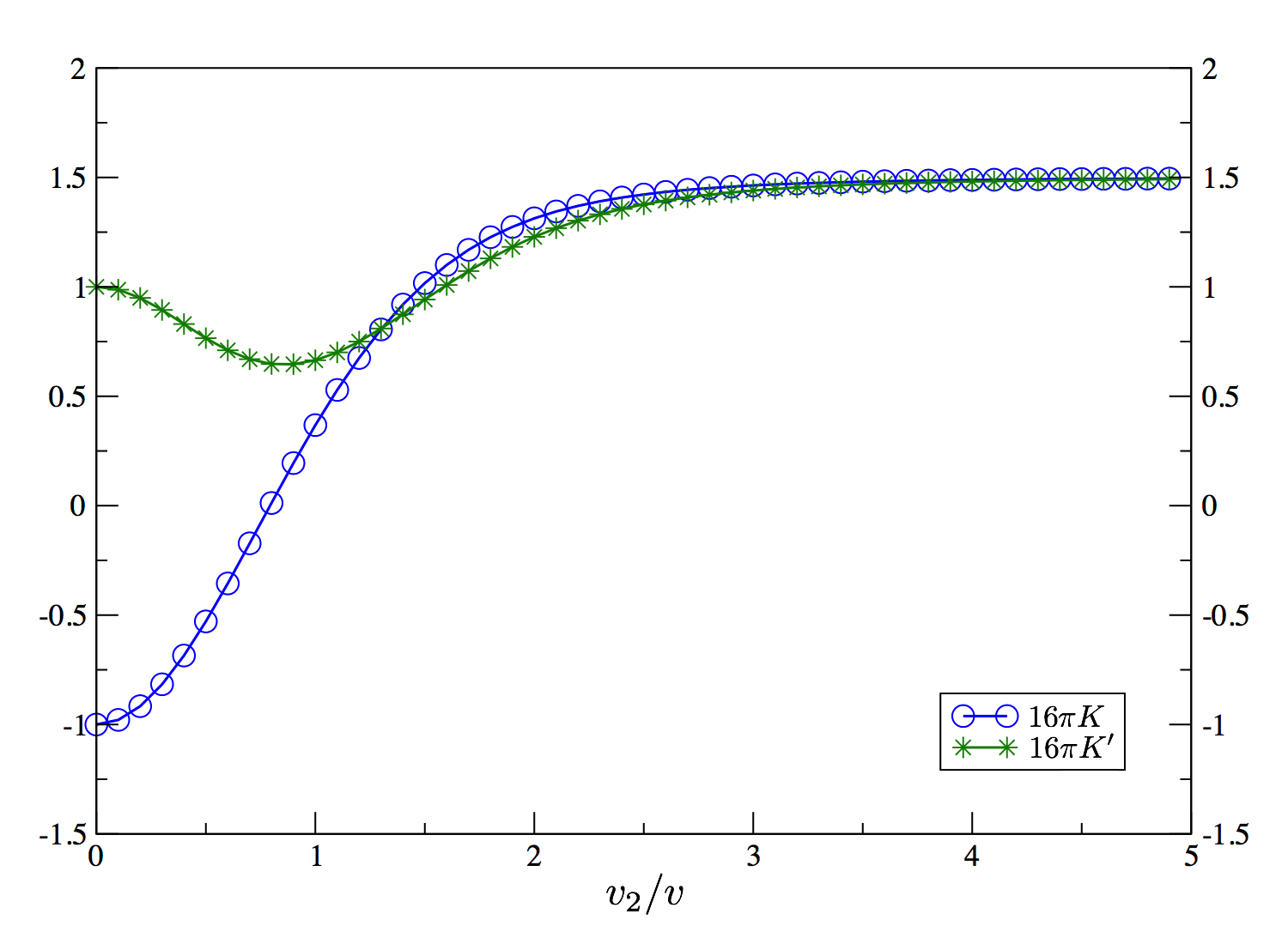
The presence of these non-zero terms supports the proposal that the general structure of the coupling between the Néel and VBS orders is the same as that in the single layer honeycomb lattice. But the values of the geometric phases differ in the weak coupling theory, although we expect them to coincide in the strong coupling theory (by the arguments of Ref. 16). This difference suggests that the weak coupling analysis points to a first-order Néel-VBS transition, while deconfined criticality is preferred at strong coupling.
VI Zero mode in VBS vortex
Another approach to the theory of deconfined criticality is via the structure of vortices in the VBS order parameter. Levin and Senthil [49] presented general arguments that each such vortex must carry spin . In some case, this fact is already apparent by the presence of zero modes in a weak coupling theory of the VBS state: this is the case in monolayer graphene [45, 46]. We present a corresponding computation for the bilayer case, and do not find such zero modes. We view this as a feature of the weak coupling approach, rather than the inapplicability of the general strong coupling arguments of Ref. 16.
We start in the deep VBS phase and may ignore the Néel order for now. Therefore we adapt the Hamiltonian Eq. 20 with . In this section we return to , and set the Fermi velocity equal to one. VBS order parameter, , now has a nonzero expectation value, and let us allow it to fluctuate over space. We will assume the fluctuation is in a much longer length scale than the lattice constant, which is set to 1, so we can treat the order parameter as a constant during Fourier transform. Moreover, we include the electric field explicitly as this will open up an energy gap of the system. The Hamiltonian in the VBS phase is,
| (31) |
where and are the Pauli matrices in valley and layer space, respectively. Note that in the bilayer graphene, the Kekulé VBS order does not open up a gap but create nodal lines which form a circle in the Brillouin zone. The nodal line is protected by the layer symmetry of the system. Discussing zero modes in a gapless system is meaningless, however, the transition is at a nonzero electric field. Electric field couples differently with the density of the electrons in different layers and breaks the layer symmetry. This opens up a gap at the nodal line and it is now legitimate to discuss zero modes of the system.
As in Sec. V, choosing a specific basis, , we can represent the Hamiltonian as a four by four matrix.
Changing to the real basis, , where for example, and ,
Here, we included into the definition of and for notational convenience and used complex coordinate for .
Now we assume the VBS order parameter contains a vortex, . Ref. 50 provides an analytical method of obtaining the zero modes when the Fermions are Dirac-like. They count the number of zero modes by matching the two asymptotic behaviors of the solutions of . The quadratic dispersion of Fermions can be easily implemented into this scheme, however, including the electric field ruins the argument and we cannot follow the same step. Alternatively, we have solved the problem numerically. We consider a bilayer honeycomb lattice with sites with the corresponding lattice Hamiltonian of Eq. 31, and introduce a vortex at the center of the lattice. Open boundary condition is imposed to deal with the vortex without including any Dirac strings. Introducing a vortex and anti-vortex pair will also resolve the issue, but it will also effectively decrease the system size. With the open boundary condition, we turn on a small potential at the boundary to eliminate zero energy states arising from boundary effects. We then numerically diagonalize the system and search for zero energy eigenvalues. We also check the eigenfunctions of the states while moving the vortex center around to confirm whether the wavefunctions are actually localized at the vortex. The result clearly showed no zero modes in the presence of a vortex. As we noted earlier, we believe this result is a feature of the weak coupling method, and that the needed zero mode will appear in the strong coupling limit as argued in Ref. 49.
We also mention previous reports about zero modes in vortices of bilayer graphene [51, 52]. In these works, the authors claim there are two zero modes for a single vortex of valley ferromagnet order. Note that this order breaks time reversal symmetry and is different from the Kekulé VBS phase we have considered above. In the notation of Eq. 31, the valley ferromagnet order will be written as , which anti-commutes with the kinetic energy terms. Ref. 52 concentrates in regions near the vortex and uses the method of Ref. 50 in momentum space. However, this is potentially dangerous because, as mentioned before, the number of zero modes are determined by the matching of the asymptotic behavior of near-vortex and far-vortex regions. Indeed, without the matching procedure, and only looking in the near-vortex region one can find an infinite number of zero modes. However by numerically diagonalizing the lattice Hamiltonian as above, we indeed find two zero modes for their system with valley ferromagnet order.
VII Conclusions
Our paper has examined the strong coupling limit of an extended Hubbard model appropriate for undoped bilayer graphene. The results of our analyses are that the application of a transverse electric field does indeed destabilize the Néel insulator, and that resulting ‘quantum disordered’ state is likely to have VBS order which breaks the space group symmetry of the lattice. These results are in accord with the weak coupling analysis [13], and our strong coupling arguments indicate that the Néel-VBS quantum phase transition in bilayer graphene can be in the deconfined universality class [17, 18].
On the experimental side, there is now good evidence for the Néel state in bilayer graphene [6, 7], and also for a quantum transition out of this state upon application of a transverse electric field [2, 3, 4]. It would be of great interest to devise experiments to measure the translational symmetry breaking associated with the VBS order. The transition to the VBS state should exhibit quantum-critical scaling, and this may be detected by a careful study of the temperature dependence of the influence of the transverse electric field on conductance across the transition, and looking for a “quantum-critical fan” [53] in the electric-field/temperature plane.
For experimental applications, the fundamental new idea that a ‘deconfined-critical’ perspective brings is that the transition out of the Néel state occurs as a consequence of condensation of low energy skyrmions in the Néel order;[17, 18] so such low energy skyrmions should be present in bilayer graphene near the transition. In the presence of ferromagnetic order, a crucial feature of skyrmions in the quantum Hall regime is that they carry electric charge.[54, 55] In the present bilayer case, each layer has intra-layer ferromagnetism in the Néel state, with opposite orientation in the two layers, and so we can expect that the layers carry opposite charges in the presence of a skyrmion. With the application of an electric field, the layer-exchange symmetry is broken, and then a skyrmion current will carry a net electrical current. It is notable that the experiments show enhanced conductivity in the region of the transition, [2] and this could be explained by the presence of low-energy skyrmions in the deconfined-critical theory. In our present strong-coupling analysis, the orbital magnetic field effects have been suppressed, and so we have not accounted for the electrical nature of the skyrmions: an extension of our analysis to include the physics of Landau levels is required, and is being undertaken. On the experimental side, the opposite layers charges carried by the skyrmion could be studied by driving currents in opposite directions in the two layers. Also, optical experiments can detect the spin-chirality fluctuations [56] linked to the collective gauge excitations of deconfined criticality; however, it will be necessary for the light to couple selectively to one layer (i.e. one sublattice of the antiferromagnet).
Acknowledgements.
We thank D. Abanin, G.-Y. Cho, D. Chowdhury, L. Fu, M. Kharitonov, Y. Huh, L.-Y. Hung, E. G. Moon, M. Punk, B. Roy, E. Shimshoni, and A. Yacoby for useful discussions. This research was supported by the NSF under Grant DMR-1103860, the Templeton foundation, and MURI grant W911NF-14-1-0003 from ARO. Research at Perimeter Institute is supported by the Government of Canada through Industry Canada and by the Province of Ontario through the Ministry of Research and Innovation. J. L. is also supported by the STX Foundation.Appendix A Geometric phases in electric field
We revisit the geometric phase calculation in Sec. V including the electric field to the Hamiltonian. As in Eq. 31, electric field couples to the layer space as an extra term. The modified Hamiltonian is,
| (40) |
The details of the calculation are the same as in Sec. V, where the only difference comes from the new Hamiltonian. The couplings and as a function of in the presence of electric fields and are shown in Fig. 7a, together with the case already in Fig. 6.


and in electric field both shows qualitatively similar behavior to the zero electric field situation. However, one should notice the quantitative values are different not only the intermediate region, but also at the and limits, where we found that the values at were quantized. The reason for this deviation is that the coupling matrices of the Néel order parameter () and of the electric field () commute, and as a result, the Néel state and the electric field induce gapped states that can mix with each other. Although they have similar dispersion in the weak coupling theory, the two states have very different topological features. For example, the gapped state by electric field does not have topological defects as skyrmions, whose geometric phase leads to nonzero and coupling terms. Explicit calculation also confirms when there is only electric field and no Néel order parameter in the theory.
We also calculate and in the bilayer () and monolayer () limit for various values of . In Fig. 7b, we see that of the bilayer limit increases as electric field increase up to . is the fine tuned value of where the energy gap vanishes. Both and diverges at this gapless point. Also, the ratios of and can be written in a simple formula. Let us write and as a function of for notational convenience. First, the and are related as,
| (41) |
when . This gives the correct limiting value for case, where . Also, as one can check roughly in Fig. 7a, strictly holds as in the limit.
References
- [1] J. G. Checkelsky, L. Li, and N. P. Ong, Phys. Rev. B 79, 115434 (2009).
- [2] R. T. Weitz, M. T. Allen, B. E. Feldman, J. Martin, and A. Yacoby, Science 330, 812 (2010).
- [3] F. Freitag, J. Trbovic, M. Weiss, and C. Schönenberger, Phys. Rev. Lett. 108, 076602 (2012).
- [4] J. Velasco, L. Jing, W. Bao, Y. Lee, P. Kratz, V. Aji, M. Bockrath, C. N. Lau, C. Varma, R. Stillwell, D. Smirnov, F. Zhang, J. Jung, and A. H. MacDonald, Nature Nanotech. 7, 156 (2012).
- [5] A. F. Young, C. R. Dean, L. Wang, H. Ren, P. Cadden-Zimansky, K. Watanabe, T. Taniguchi, J. Hone, K. L. Shepard and P. Kim, Nature Phys. 8, 550 (2012).
- [6] P. Maher, C. R. Dean, A. F. Young, T. Taniguchi, K. Watanabe, K. L. Shepard, J. Hone and P. Kim, Nature Phys. 9, 154 (2013).
- [7] F. Freitag, M. Weiss, R. Maurand, J. Trbovic, and C. Schönenberger Phys. Rev. B 87, 161402(R) (2013).
- [8] A. F. Young, J. D. Sanchez-Yamagishi, B. Hunt, S. H. Choi, K. Watanabe, T. Taniguchi, R. C. Ashoori, and P. Jarillo-Herrero, Nature, 505, 528 (2014).
- [9] V. Cvetkovic, R. E. Throckmorton, and O. Vafek, Phys. Rev. B 86, 075467 (2012).
- [10] Fan Zhang, Hongki Min, and A. H. MacDonald, Phys. Rev. B 86, 155128 (2012).
- [11] R. Nandkishore and L. Levitov, Phys. Rev. B 82, 115431 (2010).
- [12] M. Kharitonov, Phys. Rev. B 85, 155439 (2012).
- [13] M. Kharitonov, Phys. Rev. Lett. 109, 046803 (2012).
- [14] M. Kharitonov, Phys. Rev. B 86, 075450 (2012).
- [15] M. Kharitonov, Phys. Rev. B 86, 195435 (2012).
- [16] N. Read and S. Sachdev, Phys. Rev. B 42, 4568 (1990).
- [17] T. Senthil, A. Vishwanath, L. Balents, S. Sachdev, and M. P. A. Fisher, Science 303, 1490 (2004).
- [18] T. Senthil, L. Balents, S. Sachdev, A. Vishwanath, and M. P. A. Fisher, Phys. Rev. B 70, 144407 (2004).
- [19] A. W. Sandvik, Phys. Rev. Lett. 98, 227202 (2007).
- [20] M. S. Block, R. G. Melko, R. K. Kaul, Phys. Rev. Lett. 111, 137202 (2013).
- [21] B. Roy, Phys. Rev. B 88, 075415 (2013).
- [22] B. Roy, Phys. Rev. B 89, 201401(R) (2014).
- [23] B. Roy, M. P. Kennett, and S. Das Sarma, arXiv:1406.5184.
- [24] L. M. Zhang, Z. Q. Li, D. N. Basov, M. M. Fogler, Z. Hao, and M.C. Martin, Phys. Rev. B 78, 235408 (2008).
- [25] A. H. MacDonald, S. M. Girvin, and D. Yoshioka, Phys. Rev. B 37, 9753 (1988).
- [26] M. Takahashi, J. Phys. C 10, 1289 (1977).
- [27] K. Hida, J. Phys. Soc. Jpn. 59, 2230 (1990).
- [28] A. W. Sandvik, A. V. Chubukov, and S. Sachdev, Phys. Rev. B 51, 16483 (1995).
- [29] A. V. Chubukov and D. K. Morr, Phys. Rev. B 52, 3521 (1995).
- [30] A. J. Millis and H. Monien, Phys. Rev. B 54, 16172 (1996).
- [31] L. Wang, K. S. D. Beach, A. W. Sandvik, Phys. Rev. B 73, 014431 (2006).
- [32] S. Sachdev, Phys. Rev. B 45, 12377 (1992).
- [33] T. C. Lang, Z. Y. Meng, M. M. Scherer, S. Uebelacker, F. F. Assaad, A. Muramatsu, C. Honerkamp, and S. Wessel, Phys. Rev. Lett. 109, 126402 (2012).
- [34] C. Cohen-Tannoudji, J. Dupont-Roc, and G. Grynberg, Atom-Photon Interactions: Basic Processes and Applications (Wiley, New York, 1992)
- [35] B. K. Clark, D. A. Abanin and S. L. Sondhi, Phys. Rev. Lett. 107, 087204 (2011).
- [36] A. F. Albuquerque, D. Schwandt, B. Hetényi, S. Capponi, M. Mambrini, and A. M. Läuchli, Phys. Rev. B 84, 024406 (2011).
- [37] R. Ganesh, J. van den Brink, and S. Nishimoto, Phys. Rev. Lett. 110, 127203 (2013).
- [38] Z. Zhu, D. A. Huse, and S. R. White, Phys. Rev. Lett. 110, 127205 (2013).
- [39] S.-S. Gong, D. N. Sheng, O. I. Motrunich, and M. P. A. Fisher, Phys. Rev. B 88, 165138 (2013).
- [40] S. Pujari, K. Damle, and F. Alet, Phys. Rev. Lett. 111, 087203 (2013).
- [41] T. C. Lang, Z. Y. Meng, A. Muramatsu, S. Wessel, and F. F. Assaad, Phys. Rev. Lett. 111, 066401 (2013).
- [42] L. Fu, S. Sachdev, and C. Xu, Phys. Rev. B 83, 165123 (2011).
- [43] H. Yao and D.-H. Lee, Phys. Rev. B 82, 245117 (2010).
- [44] E. McCann and V. I. FalÕko, Phys. Rev. Lett. 96, 086805 (2006).
- [45] C.-Y. Hou, C. Chamon, and C. Mudry, Phys. Rev. Lett. 98, 186809 (2007).
- [46] C.-Y. Hou, C. Chamon, and C. Mudry, Phys. Rev. B 81, 075427 (2010).
- [47] A. G. Abanov and P. B. Wiegmann, Nucl. Phys. B 570, 685 (2000).
- [48] T. Senthil and M. P. A. Fisher, Phys. Rev. B 74, 064405 (2006).
- [49] M. Levin and T. Senthil, Phys. Rev. B 70, 220403(R) (2004).
- [50] R. Jackiw and P. Rossi, Nucl. Phys. B190, 681 (1981).
- [51] E.-G. Moon, Phys. Rev. B 85, 245123 (2012).
- [52] C.-K. Lu and I. F. Herbut, Phys. Rev. Lett. 108, 266402 (2012).
- [53] S. Sachdev and B. Keimer, “Quantum Criticality,” Physics Today 64, no. 2, 29 (2011).
- [54] D.-H. Lee and C. L. Kane, Phys. Rev. Lett. 64, 1313 (1990).
- [55] S. L. Sondhi, A. Karlhede, S. A. Kivelson, and E. H. Rezayi, Phys. Rev. B 47, 16 419 (1993).
- [56] P. A. Lee and N. Nagaosa, Phys. Rev. B 46, 5621 (1992).