Rigorous Uniform Approximation of D-finite Functions Using Chebyshev Expansions Thanks: This research was partly supported by the Austria Science Fund (FWF) grants P22748-N18 and Y464-N18, and before that by the MSR-Inria joint research center. Thanks: This work is in the public domain. As such, it is not subject to copyright. Where it is not legally possible to consider this work as released into the public domain, any entity is granted the right to use this work for any purpose, without any conditions, unless such conditions are required by law.
Abstract.
A wide range of numerical methods exists for computing polynomial approximations of solutions of ordinary differential equations based on Chebyshev series expansions or Chebyshev interpolation polynomials. We consider the application of such methods in the context of rigorous computing (where we need guarantees on the accuracy of the result), and from the complexity point of view.
It is well-known that the order- truncation of the Chebyshev expansion of a function over a given interval is a near-best uniform polynomial approximation of the function on that interval. In the case of solutions of linear differential equations with polynomial coefficients, the coefficients of the expansions obey linear recurrence relations with polynomial coefficients. Unfortunately, these recurrences do not lend themselves to a direct recursive computation of the coefficients, owing among other things to a lack of initial conditions.
We show how they can nevertheless be used, as part of a validated process, to compute good uniform approximations of D-finite functions together with rigorous error bounds, and we study the complexity of the resulting algorithms. Our approach is based on a new view of a classical numerical method going back to Clenshaw, combined with a functional enclosure method.
Key words and phrases:
Rigorous computing, computer algebra, complexity, D-finite functions, recurrence relation, Chebyshev series, Clenshaw method, Miller algorithm, asymptotics, functional enclosure2000 Mathematics Subject Classification
68W30, 33C45, 65L05, 65G20,1. Introduction
1.1. Background
Many of the special functions commonly used in areas such as mathematical physics are so-called D-finite functions, that is, solutions of linear ordinary differential equations (LODE) with polynomial coefficients [56]. This property allows for a uniform theoretic and algorithmic treatment of these functions, an idea that was recognized long ago in Numerical Analysis [34, p. 464], and more recently found many applications in the context of Symbolic Computation [67, 54, 32]. The present article is devoted to the following problem.
Problem 1.1.
Let be a D-finite function specified by a linear differential equation with polynomial coefficients and initial conditions. Let . Given and , find the coefficients of a polynomial written on the Chebyshev basis , together with a “small” bound such that for all .
Approximations over other real or complex segments (written on the Chebyshev basis adapted to the segment) are reduced to approximations on by means of an affine change of variables, which preserves D-finiteness.
A first motivation for studying this problem comes from repeated evaluations. Computations with mathematical functions often require the ability to evaluate a given function at many points lying on an interval, usually with moderate precision. Examples include plotting, numerical integration, and interpolation. A standard approach to address this need resorts to polynomial approximations of . We deem it useful to support working with arbitrary D-finite functions in a computer algebra system. Hence, it makes sense to ask for good uniform polynomial approximations of these functions on intervals. Rigorous error bounds are necessary in order for the whole computation to yield a rigorous result.
Besides easy numerical evaluation, polynomial approximations provide a convenient representation of continuous functions on which comprehensive arithmetics including addition, multiplication, composition and integration may be defined. Compared to the exact representation of D-finite functions by differential equations, the representation by polynomial approximations is only approximate, but it applies to a wider class of functions and operations on these functions. When we are working over an interval, it is natural for a variety of reasons to write the polynomials on the Chebyshev basis rather than the monomial basis. In particular, the truncations that occur during most arithmetic operations then maintain good uniform approximation properties. Trefethen et al.’s Chebfun [58, 17] is a popular numerical computation system based on this idea.
In a yet more general setting, Epstein, Miranker and Rivlin developed a so-called “ultra-arithmetic” for functions that parallels floating-point arithmetic for real numbers [20, 21, 30]. Various generalized Fourier series, including Chebyshev series, play the role of floating-point numbers. Ultra-arithmetic also comprises a function space counterpart of interval arithmetic, based on truncated series with interval coefficients and rigorous remainder bounds. This line of approach was revived with the introduction of “ChebModels” in recent work by Brisebarre and Joldeș [10]. Part of the motivation for Problem 1.1 is to allow one to use arbitrary D-finite functions as “base functions” at the leaves of expression trees to be evaluated using ChebModels.
Finally, perhaps the main appeal of ultra-arithmetic and related techniques is the ability to solve functional equations rigorously using enclosure methods [44, 30, 37, 45, 60]. LODE with polynomial coefficients are among the simplest equations to which these tools apply. A third goal of this article is to begin the study of the complexity of validated enclosure methods, from a computer algebra point of view, using this simple family of problems as a prototype.
1.2. Setting
To specify the D-finite function , we fix a linear homogeneous differential equation of order with polynomial coefficients
| (1.1) |
We also write . Up to a change of variable, we assume that we are seeking a polynomial approximation of a solution of (1.1) over the interval . The uniform norm on this interval is denoted by . We also assume that for , so that (by Cauchy’s existence theorem for complex LODE) all solutions of (1.1) are analytic on . Besides the operator , we are given initial values
| (1.2) |
Many of the results actually extend to the case of boundary conditions, since we can compute a whole basis of solutions of (1.1) and reduce boundary value problems to initial value problems by linear algebra. Also note that the case of initial values given outside the domain of expansion may be reduced to our setting using numerical analytic continuation.
| coefficients of the operator ; | p. 1.1 | |
| coefficients of the operator | p. ii | |
| sequences in with exponential decrease | p. 2.1 | |
| differentiation operator, | p. 1.2 | |
| differential operator, | p. 1.1 | |
| initial values, | p. 1.2 | |
| Chebyshev recurrence operator | p. 2.1, p. 2.5 | |
| degree- minimax polynomial approximation of | p. 2.1 | |
| truncated Chebyshev expansion operator | p. 2.1 | |
| order of | p. 1.1 | |
| shift operator, | p. 2.2 | |
| (usually) half-order of | p. ii, p. 3.4 | |
| singularities of , shifted by | p. 4.1 | |
| Chebyshev polynomials of the first kind | p. 2.1 | |
| (usually) unknown function, | p. 1.1, p. 5.1 | |
| approximation of computed by Algorithm 4.2 | p. 4.2 | |
| inverse Joukowski transform of a function | p. 2.1 | |
| integer interval, | p. 1.2 |
Table 1 summarizes for quick reference the notation used throughout this article. Notations related to Chebyshev expansions are detailed in Section 2.1 below. Notations from Theorem 2.1 are also repeatedly used in the subsequent discussion. Double brackets denote integer intervals .
Unless otherwise noted, we assume for simplicity that all computations are carried out in exact (rational) arithmetic. The rigor of the computation is unaffected if exact arithmetic is replaced by floating-point arithmetic in Algorithm 4.2 and by interval arithmetic in Algorithm 6.5. (In the case of Algorithm 5.6, switching to interval arithmetic requires some adjustments.) However, we do not analyze the effect of rounding errors on the quality of the approximation polynomial and error bound from Problem 1.1 when the computations are done in floating-point arithmetic. In simple cases at least, we expect that Algorithm 4.2 exhibits comparable stability to similar methods based on backward recurrence [65]. Our experiments show a satisfactory numerical behaviour.
To account for this variability in the underlying arithmetic, we assess the complexity of the algorithms in the arithmetic model. In other words, we only count field operations in , while neglecting both the size of their operands and the cost of accessory control operations. The choice of the arithmetic complexity model for an algorithm involving multiple precision numerical computations may come as surprising. Observe however that all arithmetic operations on both rational and floating-point numbers of bit size bounded by may be done in time (see for instance Brent and Zimmermann’s book [9] for detail). In general, the maximum bit size of the numbers we manipulate is roughly the same as that of the coefficients of , which may be checked to be when represented as rational numbers, so that the bit complexity of the algorithm is actually almost linear in the total bit size of the output.
1.3. Summary of Results
As we will see in the next section, truncated Chebyshev expansions of analytic functions provide very good approximations of these functions over straight line segments. In the case of D-finite functions, their coefficients are known to satisfy linear recurrences. But computing Chebyshev series based on these recurrences is not entirely straightforward.
Roughly speaking, the conclusion of the present article is that these recurrences can nevertheless be used to solve Problem 1.1 efficiently for arbitrary D-finite functions. The techniques we use (backward recurrence and enclosure of solutions of fixed-points equations in function spaces) date back to the 1950s–1960s. The originality of this work is that we insist on providing algorithms that apply to a well-defined class of functions (as opposed to methods to be adapted to each specific example), and focus on controlling the computational complexity of these algorithms.
Our algorithm proceeds in two stages. We first compute a candidate approximation polynomial, based on the Chebyshev expansion of the function . No attempt is made to control the errors rigorously at this point. We then validate the output using an enclosure method.
The main results of this article are Theorems 4.4 (p. 4.4) and 6.6 (p. 6.6), stating respectively that each of these two steps can be performed in linear arithmetic complexity with respect to natural parameters, and estimating the quality of the results they return. Theorem 4.4 is based on a description of the solution space of the recurrence on Chebyshev coefficients that is more complete than what we could find in the literature and may be of independent interest.
1.4. Outline
This article is organized as follows. In Section 2, we review properties of Chebyshev series of D-finite functions and then study the recurrence relations satisfied by the coefficients of these series, whose use is key to the linear time complexity. Section 3 provides results on the asymptotics of solutions of these recurrences that will be critical for the computation of the coefficients. The actual algorithm for this task, described in Section 4, reminds of Fox and Parker’s variant [23, Chap. 5] of Clenshaw’s algorithm [16]. A short description of a prototype implementation and several examples follow.
The part dedicated to the validation step starts in Section 5 with a study of Chebyshev series expansions of rational functions. Most importantly, we state remainder bounds that are then used in Section 6, along with an enclosure method for differential equations, to validate the output of the first stage and obtain the bound . We conclude with examples of error bounds obtained using our implementation of the validation algorithm, and some open questions.
2. Chebyshev Expansions of D-finite Functions
2.1. Chebyshev Series
Recall that the Chebyshev polynomials of the first kind are polynomials defined for all by the relation . They satisfy for all . The family is a sequence of orthogonal polynomials over with respect to the weight function , and hence a Hilbert basis of the space . (We refer the reader to books such as Rivlin’s [53] or Mason and Handscomb’s [39] for proofs of the results collected in this section.)
Expansions of functions on this basis are known as Chebyshev series. Instead of the more common
| (2.1) |
we write Chebyshev series as
| (2.2) |
This choice makes the link between Chebyshev and Laurent expansions as well as the action of recurrence operators on the (both discussed below) more transparent. The Chebyshev coefficients of the expansion of a function are given by
| (2.3) |
for all . The series (2.2) converges to in the sense for all (see for example [39, Chap. 5.3.1]). We denote by the associated orthogonal projection on the subspace of polynomials of degree at most .
Now assume that is a solution of Equation (1.1). As such, it may be analytically continued to any domain that does not contain any singular point of the equation. Let
| (2.4) |
be the largest elliptic domain with foci in with this property. Since the singular points are in finite number, we have . The coefficients then satisfy for all ; and the Chebyshev expansion (2.2) of converges uniformly to on [39, Theorem 5.16]. Letting and , it is not hard to see that the are also the coefficients of the (doubly infinite) Laurent expansion of the function around the unit circle. The transformation sending to is known as the inverse Joukowski transform. It maps the elliptic disk to the annulus
The formula translates into . The coefficients are also related to those of the Fourier cosine expansion of .
Let be the vector space of doubly infinite sequences such that
The sequence of Chebyshev coefficients of a function that is analytic on some complex neighborhood of belongs to . Conversely, for all , the function series converges uniformly on (some neighborhood of) to an analytic function .
Truncated Chebyshev series are near-minimax approximations: indeed, they satisfy [59, Theorem 16.1]
| (2.5) |
where is the polynomial of degree at most that minimizes .
Even though itself can be computed to arbitrary precision using the Remez algorithm [12, Chap. 3], Equation (2.5) shows that we do not lose much by replacing it by . Moreover, tighter approximations are typically hard to validate without resorting to intermediate approximations of higher degree [13]. The need for such intermediate approximations is actually part of the motivation that led to the present work. There exist a variety of other near-minimax approximations with nice analytical properties, e.g., Chebyshev interpolation polynomials. Our choice of truncated Chebyshev expansions is based primarily on the existence of a recurrence relation on the coefficients when is a D-finite function.
2.2. The Chebyshev Recurrence Relation
The polynomials satisfy the three-term recurrence
| (2.6) |
as well as the mixed differential-difference relation
| (2.7) |
which translates into the integration formula where . From these equalities follows the key ingredient of the approach developed in this article, namely that the Chebyshev coefficients of a D-finite function obey a linear recurrence with polynomial coefficients. This fact was observed by Fox and Parker [22, 23] in special cases and later proved in general by Paszkowski [49]. Properties of this recurrence and generalizations to other orthogonal polynomial bases were explored in a series of papers by Lewanowicz starting 1976 (see in particular [35, 36]). The automatic determination of this recurrence in a symbolic computation system was first studied by Geddes [24].
The following theorem summarizes results regarding this recurrence, extracted from existing work [49, 35, 36, 52, 4] and extended to fit our purposes. Here and in the sequel, we denote by the skew Laurent polynomial ring over in the indeterminate , subject to the commutation rules
| (2.8) |
Likewise, is the subring of noncommutative Laurent polynomials in themselves with polynomial coefficients. The elements of identify naturally with linear recurrence operators through the left action of on defined by and . Recall that denotes the differential operator appearing in Equation (1.1).
Theorem 2.1.
[49, 35, 36, 52, 4] Let be analytic functions on some complex neighborhood of the segment , with Chebyshev expansions
There exist difference operators with the following properties.
- (i)
The differential equation is satisfied if and only if
(2.9) - (ii)
The left-hand side operator is of the form where and for all .
- (iii)
Letting
(2.10) we have (this expression is to be interpreted as a polynomial identity in ). In particular, depends only on and satisfies the same symmetry property as .
Note that , as defined in Eq. (2.10), may be interpreted as an operator from the symmetric sequences to the sequences defined only for nonzero . A sloppy but perhaps more intuitive statement of the main point of Theorem 2.1 would be: “ if and only if , up to some integration constants”.
Proof.
Assume . Benoit and Salvy [4, Theorem 1] give a simple proof that (2.9) holds for some . The fact that and can actually be taken to have polynomial coefficients and satisfy the properties listed in the last two items then follows from the explicit construction discussed in Section 4.1 of their article, based on Paszkowski’s algorithm [49, 35]. More precisely, multiplying both members of [4, Eq. (17)] by yields a recurrence of the prescribed form. The recurrence has polynomial coefficients since . Rebillard’s thesis [52, Section 4.1] contains detailed proofs of this last observation and of all assertions of Item ii. Note that, although Rebillard’s and Benoit and Salvy’s works are closest to the formalism we use, several of these results actually go back to [49, 35, 36].
There remains to prove the “if” direction. Consider sequences such that , and let be the Chebyshev coefficient sequence of the (analytic) function . We then have by the previous argument. This implies , whence finally by Lemma 2.2 below. ∎
Lemma 2.2.
The restriction to of the operator from Theorem 2.1 is injective.
Proof.
With the notation of Theorem 2.1, we show by induction on that
| (2.11) |
First, we have since any sequence belonging to converges to zero as . Now assume that (2.11) holds, and let be such that for . Let . Observe that is stable under the action of , so . Since , we have
Hence, for , it holds that
| (2.12) |
Unless is ultimately zero, this implies that as , which contradicts the fact that . It follows that for large enough, and, using (2.12) again, that as soon as . Applying the hypothesis (2.11) concludes the induction. ∎
An easy-to-explain way of computing a recurrence of the form (2.9) is as follows. We first perform the change of variable in the differential equation (1.1). Then, we compute a recurrence on the Laurent coefficients of by the classical (Frobenius) method.
Example 2.3.
The function satisfies the homogeneous equation . The substitutions
yield (after clearing common factors and denominators)
We then set and extract the coefficient of (which amounts to replacing by and by ) to get the recurrence
Benoit and Salvy [4] give a unified presentation of several alternative algorithms, including Paszkowski’s, by interpreting them as various ways to perform the substitution , in a suitable non-commutative division algebra. In our setting where the operator is nonsingular over , they prove that all these algorithms compute the same operator .
Remark 2.4.
As applied in Example 2.3, the method based on setting in the differential equation does not always yield the same operator as Paszkowski’s algorithm. It can be modified to do so as follows: instead of clearing the denominator of the differential equation in given by the rational substitution, move this denominator to the right-hand side, translate both members into recurrences, and then remove a possible common left divisor of the resulting operators .
Definition 2.5.
Remark 2.6.
By Theorem 2.1(ii) and with its notation, for any sequence , we have the equalities
that is, . In particular, if is a solution of a homogeneous Chebyshev recurrence, then so is , and is a symmetric solution. Not all solutions are symmetric. For instance, the differential equation corresponds to the recurrence which allows for .
2.3. Solutions of the Chebyshev Recurrence
Several difficulties arise when trying to use the Chebyshev recurrence to compute the Chebyshev coefficients.
A first issue is related to initial conditions. Here it may be worth contrasting the situation with the more familiar case of the solution of differential equations in power series. Unlike the first few Taylor coefficients of , the Chebyshev coefficients that could serve as initial conditions for the recurrence are not related in any direct way to initial or boundary conditions of the differential equation. In particular, as can be seen from Theorem 2.1 above, the order of the recurrence is larger than that of the differential equation except for degenerate cases. Hence we need to somehow ‘‘obtain more initial values for the recurrence than we naturally have at hand’’ 11 1 Nevertheless, the recurrence (2.9) shows that the Chebyshev coefficients of a D-finite function are rational linear combinations of a finite number of integrals of the form (2.3). Computing these coefficients efficiently with high accuracy is an interesting problem to which we hope to come back in future work. See Benoit [3] for some results..
Next, also in contrast to the case of power series, the leading and trailing coefficients of the recurrence (2.9) may vanish for arbitrarily large values of even though the differential equation (1.1) is nonsingular. The zeroes of are called the leading singularities of (2.9), those of , its trailing singularities. In the case of Chebyshev recurrences, leading and trailing singularity sets are opposite of each other.
One reason for the presence of (trailing) singularities is clear: if a polynomial of degree is a solution of , then necessarily . However, even differential equations without polynomial solutions can have arbitrarily large leading and trailing singularities, as shown by the following example.
Example 2.7.
For all , the Chebyshev recurrence relation associated to the differential equation , namely
admits the leading singularity . For , the differential equation has no polynomial solution.
We do however have some control over the singularities.
Proposition 2.8.
With the notations of Theorem 2.1, the coefficients of the Chebyshev recurrence satisfy the relations
| (2.13) |
with for . In particular, is zero for all .
Proof.
We proceed by induction on . When , assertion (2.13) reduces to , which follows from the second item of Theorem 2.1. In particular, this proves the result for . Now let and assume that the proposition holds when has order . Write where and is a differential operator of order at most . Letting be the Chebyshev recurrence operator associated to , we then have [4]
| (2.14) |
where the last term denotes the evaluation of at . Since
by the commutation rule (2.8), relation (2.14) rewrites as
The case having already been dealt with, assume . Since and is a polynomial, it follows by extracting the coefficient of in the last equality and evaluating at that
| (2.15) |
Now for by the induction hypothesis, and the term involving vanishes for and . In each case, we obtain . ∎
Corollary 2.9.
Let be the Chebyshev recurrence operator associated to . The image by of a symmetric sequence satisfies for .
Proof.
Last but not least, Chebyshev recurrences always admit divergent solution sequences. Divergent solutions do not correspond to the expansions of solutions of the differential equation the recurrence comes from.
Example 2.10.
The Chebyshev recurrence associated to the equation is
In terms of the modified Bessel functions and , a basis of solutions of the recurrence is given by the sequences and . The former is the coefficient sequence of the Chebyshev expansion of the exponential function and decreases as . The later satisfies .
3. Convergent and Divergent Solutions
3.1. Elements of Birkhoff-Trjitzinsky Theory
Before studying in more detail the convergent and divergent solutions of the Chebyshev recurrence relation, we recall some elements of the asymptotic theory of linear difference equations. Much of the presentation is based on Wimp’s book [65, Appendix B], to which we refer the reader for more information.
Definition 3.1.
For all , , , we call the formal expansion
| (3.1) |
where
a formal asymptotic series (FAS). The set of all FAS is denoted by .
Formal asymptotic series are to be interpreted as asymptotic expansions of sequences as . The product of two FAS is defined in the obvious way and is again an FAS. The same goes for the substitution for fixed , using identities such as . The sum of two FAS is not always an FAS, but that of two FAS sharing the same parameters is. Thus, it makes sense to say that an FAS satisfies a recurrence
| (3.2) |
with formal series coefficients of the form
| (3.3) |
Also, given FAS , the Casoratian
belongs to as well.
Following Wimp, we say that are formally linearly independent when their Casoratian is nonzero. Note that the elements of any subset of are then formally linearly independent as well. Indeed, it can be checked by induction on that FAS are formally linearly dependent if and only if there exists a relation of the form where the are FAS such that22 2 Like Wimp, but unlike most authors, we consider recurrences rather than difference equations. Accordingly, we forbid factors of the form with in (3.1), so that the are actually constants in our setting. .
Definition 3.2.
The FAS (3.1) is said to be an asymptotic expansion of a sequence , and we write , when for any truncation order , the relation
holds as .
The following fundamental result is known as the Birkhoff-Trjitzinsky theorem, or “main asymptotic existence theorem” for linear recurrences. It will be the starting point of our analysis of the computation of “convergent” solutions of the Chebyshev recurrence by backward recurrence.
Theorem 3.3.
We note that many expositions of the Birkhoff-Trjitzinsky theorem warn about possible major gaps in its original proof. However, the consensus among specialists now appears to be that these issues have been resolved in modern proofs [27, 62]. Besides, under mild additional assumptions on the Chebyshev recurrence, all the information needed in our analysis is already provided by the more elementary Perron-Kreuser theorem33 3 The Perron-Kreuser theorem yields the existence of a basis of solutions such that , under the assumption that . It does not require that the coefficients of (3.4) admit full asymptotic expansions, which makes it stronger than Theorem 3.3 in some respects. (cf. [26, 41, 43]) or its extensions by Schäfke [55]. See also Immink [28] and the references therein for an alternative approach in the case of recurrences with polynomial coefficients, originating in unpublished work by Ramis.
Also observe that for any subfamily of the sequences from Theorem 3.3, the matrix is nonsingular for large . In particular, the can vanish only for finitely many . The more precise statement below will be useful in the sequel.
Lemma 3.4.
Assume that the sequences admit formally linearly independent asymptotic expansions of the form (3.1), with , . Then the Casorati determinant
satisfies
for some , , and .
Proof.
Write . The formal linear independence hypothesis means that , and hence , admit nonzero FAS as asymptotic expansions. Additionally,
has at most polynomial growth, so that the leading term of its asymptotic expansion must be of the form . ∎
3.2. Newton Polygon of a Chebyshev Recurrence
The formal solutions described in Theorem 3.3 may be constructed algorithmically using methods going back to Poincaré [50] and developed by many authors. See in particular Adams [1] and Birkhoff [6] for early history, Tournier [57] for a comparison of several methods from a Computer Algebra perspective, and Balser and Bothner [2] for a modern algorithm as well as more references.
Here, we are mostly interested in the parameters and that control the “exponential” growth rate of the solutions. We briefly recall how the possible values of these parameters are read off the recurrence using the method of Newton polygons. Consider again the Chebyshev recurrence operator
from Section 2.2. The Newton polygon of is defined as the lower convex hull of the points (see Figure 1). To each edge of the polygon is attached a characteristic equation
where denotes the leading coefficient of . Note that the degrees of the sum to . Let
be the sequence of all roots of the polynomials , with multiplicities, the roots corresponding to distinct edges being written in the order of increasing and the roots of each in that of increasing modulus. For all , let be the slope of the edge associated to . (Thus, each is repeated a number of times equal to the horizontal length of the corresponding edge, and we have .)
How does this relate to the asymptotics of Chebyshev series? Assume that is the leading factor of some FAS solution of . It is not too hard to see that, in order for asymptotically dominant terms of to cancel out, must be among the slopes of the Newton polygon of , and must be a root of the characteristic equation of the corresponding edge. This gives all possible values of and . Conversely, the construction behind Theorem 3.3 (i) yields a number of linearly independent FAS with given and equal to the multiplicity of as a root of the characteristic equation of the edge of slope . In the case of Chebyshev recurrences, the Newton polygon has the following symmetry property.
Proposition 3.5.
The slopes of the Newton polygon of and the roots of its characteristic equations satisfy and for all . In addition, none of the roots associated to the horizontal edge (if there is one) has modulus .
Proof.
By Theorem 2.1, the coefficients of are related by . Hence, the Newton polygon is symmetric with respect to the vertical axis, and for all . Now fix , and let be the edge of slope . The characteristic equation of reads
where denotes the leading coefficient of a polynomial . Using the relation for lying on , we get
and hence .
There remains to prove that implies . Under the change of variable , the leading term with respect to of is . (The leading term is well-defined because the commutation relation between and preserves degrees.) Therefore, the characteristic equation associated to the slope (when there is one) of the recurrence operator obtained by changing into and into is
where is the leading coefficient of (1.1). Since is a right factor of , the characteristic polynomial associated to in the Newton polygon of divides . But, due to the assumptions stated in Section 1.2, the polynomial does not vanish for , hence for . ∎
Summing up, the asymptotic structure of the solutions of the Chebyshev recurrence may be described as follows. Similar observations were already made by Rebillard [52, Chap. 5].
Corollary 3.6.
For large enough , the space of sequences satisfying (“germs of solution at infinity of the Chebyshev recurrence”) has a basis comprising convergent sequences and divergent sequences , all with formally linearly independent FAS expansions, such that
In particular, we have for all .
4. Computing Approximation Polynomials
4.1. Clenshaw’s Algorithm Revisited
At this point, we know that Chebyshev expansions of D-finite functions correspond to the symmetric, convergent solutions of the Chebyshev recurrences introduced in Section 2.2. The question we now face is to compute these solutions efficiently in spite of the various difficulties discussed above. Our algorithm for this task may be viewed as a systematized variant of a method originally due to Clenshaw [16]. The link between Clenshaw’s method44 4 The Clenshaw method we are referring to in this text should not be confused with the Horner-like scheme for Chebyshev polynomials known as Clenshaw’s algorithm [15]. and the Chebyshev recurrence was observed long ago by Fox and Parker [22, 23] and further discussed by Rebillard [52, Section 4.1.3]. Based on the properties of the recurrence established in the last two sections, we can turn Clenshaw’s method into a true algorithm that applies uniformly to differential equations of arbitrary order and degree.
Both Clenshaw’s original method and our algorithm are related to Miller’s well-known backward recurrence technique [5, 65] to compute minimal (“slowest increasing”) solutions of three-term recurrences. Miller’s idea is to compute the coefficients of a linear recurrence sequence in the backward direction, starting form arbitrary “initial conditions” and . When goes to infinity ( being chosen once and for all), the computed coefficients get close to those of a minimal solution with large , in accordance with the intuition that “minimal solutions are the dominant ones when going backwards”. This method behaves much better numerically that the standard forward recurrence. But its key feature for our purposes is that it allows one to compute a minimal solution characterized by its minimality plus one normalizing condition instead of two initial values.
Roughly speaking, our method amounts to a “block Miller algorithm” tuned to the special case of Chebyshev recurrences. We use the idea of backward recurrence to approximate the whole subspace of convergent solutions instead of a single minimal one. There remains to take care of the constraints related to the singularities of the recurrence, the symmetry condition and the initial values of the differential equation, all of which is done using linear algebra.
Denote . Let
be the space of symmetric sequences whose restriction to satisfies the Chebyshev recurrence, except possibly when .
Proposition 4.1.
- (i)
The space of symmetric sequences such that has dimension . Among the elements of , these sequences are characterized by the linear equations
(4.1) These equations are linearly independent.
- (ii)
Proof.
First observe that a sequence automatically satisfies for too, by Remark 2.6. Then belongs to if and only if for and for . But the equations with are trivial by Corollary 2.9, thus if and only if and (4.1) is satisfied.
Let , and let denote the rank of (4.1), considered as a system of linear forms over . For large enough , sequences are in bijection with their values , where , hence has dimension . It follows that .
Similarly, an element of is characterized, for large , by a convergent sequence (“a convergent germ of solution”) and values for . It belongs to when additionally (4.1) is satisfied. Thus, by Corollary 3.6, we have and , where is the rank of the system (4.1) restricted to . But we already know from Theorem 2.1 that , and hence . Therefore, we have , and hence . ∎
The important fact is that the equations (4.1) are independent. The other statements are there to complete the picture but are not really used in the sequel. Incidentally, Proposition 4.1 implies that divergent solutions of a Chebyshev recurrence have the same exponential growth near positive and negative infinity.
The full procedure is stated as Algorithm 4.2. As the handling of boundary conditions is naturally incorporated into the algorithm, here, we see the initial conditions as a special case of boundary conditions
| (4.2) |
each of the form with and . In general, the boundary conditions are assumed to be chosen so that the function of interest is the unique solution of (1.1) satisfying (4.2). They are independent in the sense that the linear forms are linearly independent.
Motivated by Proposition 4.1, we “unroll” linearly independent test sequences . We then solve the linear system (4.3), consisting of the constraints (4.1) and of approximations of the boundary conditions (4.2), to select a single linear combination of the as output. Algorithm 4.2 takes as input both a target degree and a starting index . We will see in the next section how the choice of influences the quality of the output. In practice, taking usually yields good results.
Algorithm 4.2.
Input: a linear differential operator of order , boundary conditions as in (4.2), a target degree , an integer . Output: an approximation of the corresponding solution of .
- 1
compute the Chebyshev recurrence operator associated to
- 2
set and
- 3
for from down to
- 4
for
- 5
if then set
- 6
else if or then set
- 7
else compute using the relation
- 5
- 4
- 8
using indeterminates , , set
- 9
solve for the linear system
(4.3) - 10
return
The complexity of Algorithm 4.2 is easy to estimate.
Proposition 4.3.
For fixed , , and , Algorithm 4.2 runs in arithmetic operations.
Its correctness is less obvious. At first sight, there could conceivably exist differential equations for which Algorithm 4.2 always fails, no matter how large is chosen. It could happen for instance that the kernel of (4.1) (a system we know to have full rank over by Proposition 4.1) always has a nontrivial intersection with . It is not clear either that, when the algorithm does return a polynomial , this polynomial is close to . We prove in the next section that these issues do not occur. But already at this point, we note that if the result happens to be satisfactory, it is already possible to validate it (that is, to get a rigorous good upper-bound on ) using the methods of Section 6.
4.2. Convergence
We now prove that Algorithm 4.2 converges. The fact that it does not fail for large will come as a byproduct of the convergence proof. The proof, inspired in part by the analysis of the generalized Miller algorithm [66, 65], is based on the asymptotic behaviour of the solutions of the Chebyshev recurrence predicted by Theorem 3.3. The approach of backward recurrence algorithms based on this theorem was pioneered by Wimp [64].
Retaining the notation from the previous subsection, assume that the operator and the boundary conditions are fixed. Write the Chebyshev expansion of as
Let , , be the coefficients computed by Algorithm 4.2 (run in exact arithmetic) when called with the starting index .
The central result of the analysis of Algorithm 4.2 is the following theorem. It implies that when is fixed and , the polynomial output by Algorithm 4.2 converges at least exponentially fast to the truncated Chebyshev series . The base of the exponential is related to the asymptotics of the “slowest decreasing” convergent solution of the Chebyshev recurrence, in turn related to the location of the singular points of the differential equation (1.1).
Theorem 4.4.
We write when there exists such that as .
Proof.
The finite sequence computed by Algorithm 4.2 extends to an element of characterized by the conditions
from Step 3, along with the linear system (4.3) solved in Step 9.
By writing the linear forms that express the boundary conditions (4.2) as , we define “truncations”
that make sense even for divergent series. (Abusing notation slightly, we apply the and indifferently to functions, formal Chebyshev series or their coefficient sequences.) The system (4.3) consists of the equations and of the symmetry and extension-through-singularities constraints (4.1). We introduce additional linear forms to write these last equations in the same form as the first , so that (4.3) becomes
| (4.4) |
Now let be a basis of the solutions of in the neighborhood of of the form provided by Corollary 3.6. Extend each to an element of , and then the tuple to a basis of by setting where are the elements of . Let
| (4.5) |
Let be the same determinant with the column involving replaced by
By Cramer’s rule, provided , the sequence decomposes on the basis of as
| (4.6) |
Algorithm 4.2 fails if and only if .
The sequence of “exact” Chebyshev coefficients of the function defined by the input is likewise given by
| (4.7) |
where
and denotes the determinant with the -th column replaced by .
Our goal is now to prove that fast as . To do that, we study the asymptotic behaviours of the determinants and .
We decompose into the four blocks indicated by Eq. (4.5) as follows:
The corresponding modified blocks in are denoted , , , . (We drop the explicit index for readability, but notice that these matrices depend on .) The blocks and are nonsingular for large , the first one by Lemma 3.4 and the second one because as . The Schur complement formula implies
Setting , the entry at position in the matrix satisfies for large if , and otherwise
(where the notation indicates the omission of the corresponding term) as by Lemma 3.4.
In view of our assumptions on the boundary conditions (4.2), we have for all , where is the maximum derivation order appearing in (4.2). Additionally, the sequences with are ultimately zero. Therefore the entries of satisfy
This yields the estimate
for the -th column of . Since
we get as well, and
In particular, for all large enough , hence, for any fixed differential equation, the algorithm fails at most for finitely many .
We turn to the modified determinants
For , the same reasoning as above (except that may now be singular) leads to
hence
| (4.8) |
In the case , write
The natural entrywise bounds on and yield and from there
so that
For however, the -th column of is zero and that of is constant, hence
It follows that
whence
| (4.9) |
Remark 4.5.
In the special case where the solution is a polynomial, it is computed exactly.
Theorem 4.4 implies that the polynomial returned by Algorithm 4.2 satisfies
| (4.10) |
where and are the asymptotic growth parameters defined in Section 3.2, for some with . Thus, given , it suffices to take in order to obtain . The constant hidden in the depends on . The estimate goes down to when , that is (by a similar argument as in the proof of Proposition 3.5), when the leading coefficient of the differential equation is a constant.
Comparing with Equation (2.5), we can state the following “effective near-minimax approximation” property.
Corollary 4.6.
Let and be fixed. Given , there exists such that Algorithm 4.2, called with parameters , , , and , computes a polynomial of degree at most satisfying in arithmetic operations.
There is a different way of looking at this, starting with the lower bound [12, Sec. 4.4, Theorem 5(i)]
| (4.11) |
on the quality of the minimax polynomial approximation of degree of a function in terms of the Chebyshev coefficients of . In the (typical) case where
| (4.12) |
we see by comparing with (4.10) that choosing is enough to get
This last inequality in turn implies
When, in (4.12), and are replaced by and for some , the estimate still holds in the case where . It becomes when either or , and in general (that is, when ).
4.3. Examples
| (i) | 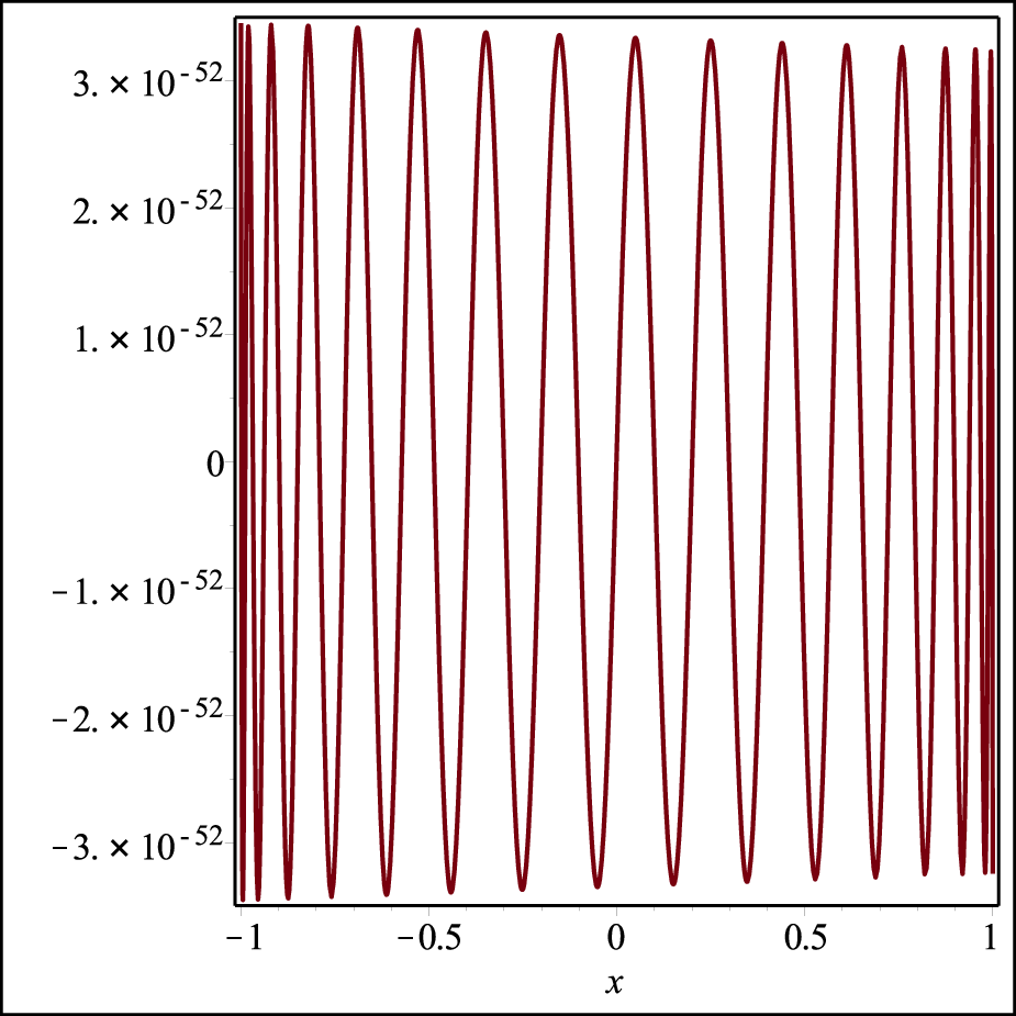 |
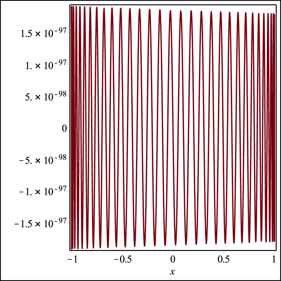 |
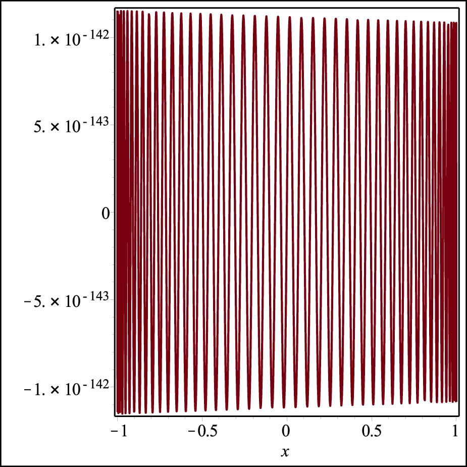 |
|---|---|---|---|
| (ii) | 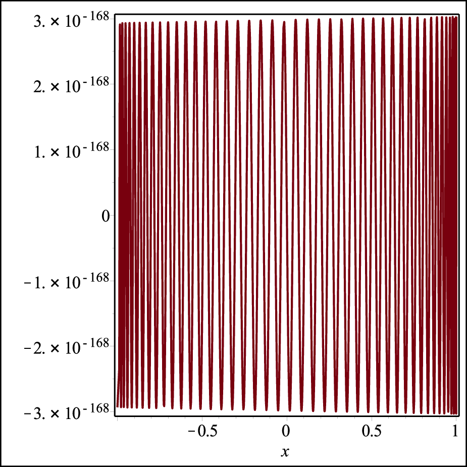 | ||
| (iii) | 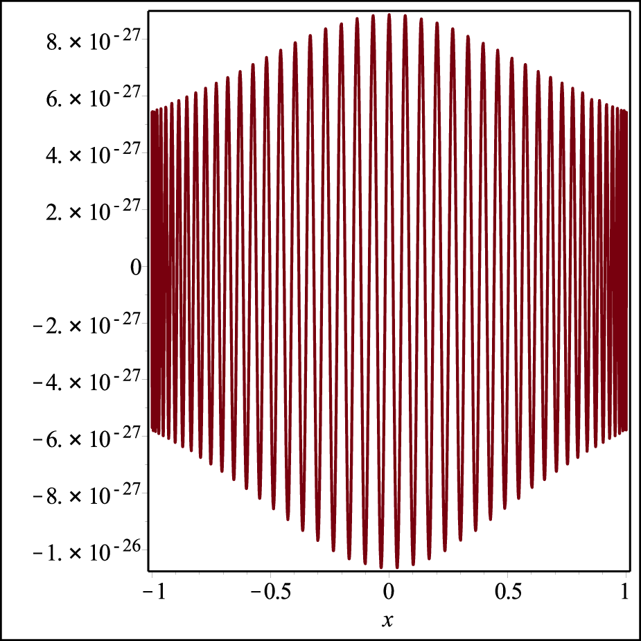 | ||
We have developed a prototype implementation of Algorithm 4.2 in Maple [38]. Our implementation uses exact rational arithmetic for operations on the coefficients of approximation polynomials. The experimental source code can be downloaded from
http://homepages.laas.fr/mmjoldes/Unifapprox
Besides Algorithm 4.2, it includes a (not entirely rigorous with respect to several minor outwards rounding issues) proof-of-concept implementation of the validation algorithm of Section 6 further discussed in that section. The gfsRecurrence package [3] available on the same web page provides tools to compute Chebyshev recurrences from linear differential equations as discussed in Section 2.2.
For each of the following examples, Figure 2 shows the graph of the difference between the polynomial approximation of a given degree computed by the implementation and the known exact solution, illustrating the quality of the approximations.
- (i)
The first example is adapted from Kaucher and Miranker [30, p. 222]. It concerns the hyperexponential function
which can be defined by the differential equation
- (ii)
Next, we consider the fourth order initial value problem (taken from Geddes [24, p. 31])
with the exact solution
- (iii)
Finally, the second-order differential equation
has complex singular points at , relatively close to the interval , and admits the exact solution
On our test system, using Maple 17, the total computation time for each example is of the order of 0.05 to 0.1 s.
According to a classical theorem of de la Vallée Poussin [12, Section 3.4], the near-uniform amplitude of the oscillation observed in the first two examples indicates an approximation error very close to that of the minimax approximation. Table 2 in Section 6.2 (p. 2) gives numerical values of and in each case. We will later extend these examples to include in the comparison the bounds on output by the validation algorithm.
4.4. A Link with the Tau Method
Besides Clenshaw’s, another popular method for the approximate computation of Chebyshev expansions is Lánczos’ tau method [33, 34]. It has been observed by Fox [22] and later in greater generality (and different language) by El Daou, Ortiz and Samara [19] that both methods are in fact equivalent, in the sense that they may be cast into a common framework and tweaked to give exactly the same result. We now outline how the use of the Chebyshev recurrence fits into the picture. This sheds another light on Algorithm 4.2 and indicates how the Chebyshev recurrence may be used in the context of the tau method.
As in the previous sections, consider a differential equation of order , with polynomial coefficients, to some solution of which a polynomial approximation of degree is sought. Assume for simplicity that there are no nontrivial polynomial solutions, i.e., .
In a nutshell, the tau method works as follows. The first step is to compute where is a polynomial of degree with indeterminate coefficients. Since , the result has degree greater than . One then introduces additional unknowns in such number that the system
| (4.13) |
has a (preferably unique) solution. The output is the value of obtained by solving this system; it is an exact solution of the projection of the original differential equation.
Now let and extend the sequence by putting for and . It follows from (4.13) that where and are the recurrence operators given by Theorem 2.1. Denoting , we also see from the explicit expression of that . Hence the coefficients of the result of the tau method are given by the Chebyshev recurrence, starting from a small number of initial conditions given near the index .
“Conversely,” consider the polynomial computed in Algorithm 4.2 with , and let . We have by Theorem 2.1. But the definition of in the algorithm also implies that when (since the , are linear combinations of sequences recursively computed using the recurrence ) or (since for ), so that . It can be checked that the Chebyshev recurrence associated to is : indeed, in the language of [4], it must be the first element of a pair satisfying . Thus is equivalent to , whence
| (4.14) |
We see that the output of Algorithm 4.2 satisfies an inhomogeneous differential equation of the form . (However, the support of the sequence itself is not sparse in general.)
This point of view also leads us to the following observation.
Proposition 4.8.
In comparison, the best known arithmetic complexity bound for the conversion of arbitrary polynomials of degree from the Chebyshev basis to the monomial basis is , where stands for the cost of polynomial multiplication [48, 8].
Proof.
As already mentioned, the Taylor series expansion of a function that satisfies an LODE with polynomial coefficients obeys a linear recurrence relation with polynomial coefficients. In the case of an inhomogeneous equation , the recurrence operator does not depend on , and the right-hand side of the recurrence is the coefficient sequence of . Now satisfies where is given by (4.14). The coefficients of (4.14) are easy to compute from the last few Chebyshev coefficients of . One deduces the coefficients in linear time by applying repeatedly the non-homogeneous recurrence relation
| (4.15) |
obtained by differentiation of the equation (2.6), and finally those of the expansion of on the monomial basis using the recurrence relation they satisfy. ∎
5. Chebyshev Expansions of Rational Functions
This section is devoted to the same problems as the rest of the article, only restricted to the case where is a rational function. We are interested in computing a recurrence relation on the coefficients of the Chebyshev expansion of a function , using this recurrence to obtain a good uniform polynomial approximation of on , and certifying the accuracy of this approximation. All this will be useful in the validation part of our main algorithm.
Our primary tool is the change of variable followed by partial fraction decomposition. Similar ideas have been used in the past with goals only slightly different from ours, like the computation of in closed form [18, 40]. Indeed, the sequence turns out to obey a recurrence with constant coefficients. Finding this recurrence or a closed form of are essentially equivalent problems. However, we will use results regarding the cost of the algorithms that do not seem to appear in the literature. Our main concern in this respect is to avoid conversions of polynomial and series from the monomial to the Chebyshev basis and back. We also need simple error bounds on the approximation of a rational function by its Chebyshev expansion.
5.1. Recurrence and Explicit Expression
Let be a rational function with no pole in . As usual, we denote by , and the symmetric Chebyshev coefficient sequences of , and .
Proposition 5.1.
The Chebyshev coefficient sequence obeys the recurrence relation with constant coefficients .
Proof.
This is actually the limit case of Theorem 2.1, but a direct proof is very easy: just write
and identify the coefficients of like powers of . ∎
As in the general case (Section 2), this recurrence has spurious (divergent) solutions besides the ones we are interested in. However, we can explicitly separate the positive powers of from the negative ones in the Laurent series expansion
| (5.1) |
using partial fraction decomposition. From the computational point of view, it is better to start with the squarefree factorization of the denominator of :
| (5.2) |
and write the full partial fraction decomposition of in the form
| (5.3) |
where . The may be computed efficiently using the Bronstein-Salvy algorithm [11] (see also [25]).
We obtain an identity of the form (5.1) by expanding the partial fractions corresponding to poles with in power series about the origin, and those with about infinity. The expansion at infinity of
converges for and does not contribute to the coefficients of , in the complete Laurent series. It follows from the uniqueness of the Laurent expansion of on the annulus that55 5 To prevent confusion, it may be worth pointing out that in the expression the Laurent expansion of a single term of the form is not symmetric for , even if .
| (5.4) |
We now extract the coefficient of in (5.4) and use the symmetry of to get an explicit expression of in terms of the roots of .
Proposition 5.2.
5.2. Truncation Error
We can now explicitly bound the error in truncating the Chebyshev expansion of .
Proposition 5.3.
Proof.
We have because for all . Using the inequality
for , the explicit expression from Proposition 5.2 yields
Since actually implies when , the asymptotic estimate follows. ∎
5.3. Computation
There remains to check that the previous results really translate into a linear time algorithm. We first state two lemmas regarding basic operations with polynomials written on the Chebyshev basis.
Lemma 5.4.
The product where the operands and the result are written in the Chebyshev basis may be computed in operations.
Proof.
It suffices to loop over the indices and, at each step, add to the coefficients of in the product the contribution coming from the coefficient of in and that of in , according to the formula . ∎
The naïve Euclidean division algorithm [63, Algorithm 2.5] runs in linear time with respect to the degree of the dividend when the divisor is fixed. Its input and output are usually represented by their coefficients in the monomial basis, but the algorithm is easily adapted to work in other polynomial bases.
Lemma 5.5.
The division with remainder () where are represented in the Chebyshev basis may be performed in operations for fixed .
Proof.
Assume . The classical polynomial division algorithm mainly relies on the fact that where and . From the multiplication formula follows the analogous inequality where , now denote the coefficients of and in the Chebyshev basis. Performing the whole computation in that basis amounts to replacing each of the assignments repeatedly done by the classical algorithm by . Since the polynomial has at most nonzero coefficients, each of these steps takes constant time with respect to . We do at most such assignments, hence the overall complexity is . ∎
We end up with Algorithm 5.6. In view of future needs, it takes as input a polynomial of arbitrary degree already written in the Chebyshev basis in addition to the rational function (of bounded degree) . The details of the algorithm are only intended to support the complexity estimates, and many improvements are possible in practice.
Algorithm 5.6.
Input: a rational fraction , the Chebyshev coefficients of a polynomial , an error bound . Output: the Chebyshev coefficients of an approximation of such that .
- 1
convert and to Chebyshev basis
- 2
compute the polynomial , working in the Chebyshev basis
- 3
compute the quotient and the remainder in the Euclidean division of by
- 4
compute the partial fraction decomposition of , where , using the Bronstein-Salvy algorithm
- 5
find such that using Proposition 5.3
- 6
compute and such that
- 7
compute
- 8
set , with
- 9
compute approximations of the roots of such that
- 10
for
- 11
set
- 11
- 12
return
Proposition 5.7.
Algorithm 5.6 is correct. As and with all other parameters fixed, it runs in arithmetic operations and returns a polynomial of degree , where depends on , but not on or .
Proof.
Firstly, we prove the error bound . Let and
On , we have
By Proposition 5.2, observing that the condition from Step 8 implies , we have the inequalities
Therefore, the output of Algorithm 5.6 satisfies
By Proposition 5.3, for all , there exists with . In addition, we have , hence the degree of the output, as computed in Step 5, satisfies .
Turning to the complexity analysis, Steps 1 and 4–8 have constant cost. So does each iteration of the final loop, assuming the powers of are computed incrementally. Steps 2 and 3 take operations by Lemmas 5.4 and 5.5, and do not depend on . Regarding Step 9, it is known [47, Theorem 1.1(d)] that the roots of a polynomial with integer coefficients can be approximated with of absolute accuracy in arithmetic operations. (In fact, the bit complexity of the algorithm beyond this statement is also softly linear in .) Since depends neither on nor on , we have , and hence the cost of Step 9 is in . ∎
6. Validation
Assume that we have computed a polynomial of degree
which presumably is a good approximation on of the D-finite function defined by (1.1,1.2). As stated in Problem 1.1, our goal is now to obtain a reasonably tight bound such that .
6.1. Principle
The main idea to compute the bound is to convert the initial value problem defining into a fixed-point equation , verify explicitly that maps some neighborhood of into itself, and conclude that must be close to the “true” solution. This is one simple instance of the functional enclosure methods mentioned in Section 1.1 and widely used in interval analysis [44]. In most cases (with the notable exception of [21, 30, 31]), these methods are based on interval Taylor series expansions such as so-called Taylor models [37, 45]. Here, we describe an adaptation designed to work in linear time with polynomial approximations written on the Chebyshev basis.
The first step is to reduce the differential initial value problem defining to a linear integral equation of the Volterra type and second kind. Let be such that
and, for , define
Observe that for all and , the operator is of the form
so that . In particular, does not vanish on .
Lemma 6.1.
The solution of such that for satisfies
| (6.1) |
where
| (6.2) |
and
| (6.3) |
Proof.
We have
Applying this formula to integrate times the equation yields
and (6.1) follows using the relation
(which can be obtained by repeated integrations by parts). ∎
Let denote the Banach space of continuous functions from to (or ), equipped with the uniform norm. With and as in Lemma 6.1, define an operator by
| (6.4) |
so that (6.1) becomes . The next proposition is an instance of a classical bound (compare, e.g., Rall [51, Chap. 1]). As we recall below, when is close to the fixed point , its iterated image remains close to , which yields good upper bounds on the distance .
Proposition 6.2.
Assume that is an upper bound on for and between and . Then the bound
holds for all .
Proof.
Let denote the linear part of . Equation (6.4) rewrites again as . More generally, we have
for all . The operator is continuous, and since
the (subordinate) norm of satisfies
Therefore, the series converges, is invertible, and . Writing
yields the announced result. ∎
The interesting fact about this bound is that we can effectively compute rigorous approximations of the right-hand side. Indeed, and are explicit polynomials, so that it is not too hard to compute approximately while keeping track of the errors we commit, and deduce a bound on its norm.
Choosing (and ) in Proposition 6.2 already yields a nontrivial estimate, but (as we shall see in more detail) larger values of are useful since as . In particular, we have
| (6.5) |
for large . This crude bound will be enough for our purposes. In practice, though, it is better to compute an approximation of that is closer to reality (e.g., using the first few terms of the series and a bound on the tail) in order to reduce the required number of iterations of .
6.2. Algorithm
The actual computation of relies on the following lemmas.
Lemma 6.3.
One can compute an antiderivative of a polynomial66 6 Note however that derivation does not commute with the truncation of Chebyshev series. of degree at most written on the Chebyshev basis in arithmetic operations.
Proof.
If and , then we have according to Equation (2.7). ∎
Lemma 6.4.
Let (with ) be a polynomial of degree , given on the Chebyshev basis. Then one can compute such that
in arithmetic operations.
Proof.
It suffices to take . Indeed, we have
It follows that
where the first inequality results from the integral expression of , the second one, from the fact that for all , and the last one from the Cauchy-Schwarz inequality. ∎
This results in Algorithm 6.5. Again here, the suggested bounds for , and are only intended to support the complexity estimate, and tighter choices are possible in practice.
Algorithm 6.5.
Input: A differential operator of order such that for , initial values . A degree- polynomial written on the Chebyshev basis. An accuracy parameter . Output: A real number such that , where is the unique solution of satisfying .
We now prove that Algorithm 6.5 works as stated, and estimate how tight the bound it returns is.
Theorem 6.6.
Algorithm 6.5 is correct: its output is an upper bound for . For fixed , as and , the bound satisfies
and the algorithm performs arithmetic operations.
Proof.
Denote by the linear part of and recall from the proof of Proposition 6.2 that . For all , the polynomial computed on line 8 satisfies
hence we have
By Proposition 6.2, it follows that
| (6.6) |
This establishes the correctness of the algorithm.
We now turn to the tightness statement. Letting , Lemma 6.4 implies that
| (6.7) |
where
| (6.8) | ||||
Looking at the definition of in step 7, we see that for some depending on only. Additionally, according to Proposition 5.7, there exists (again depending on only) such that It follows by induction that for all , whence
| (6.9) |
Plugging (6.8) and (6.9) into (6.7) yields the estimate
| (6.10) |
and the result then follows from the definition of since .
Finally, the only steps whose cost depends on or are lines 7, 8, and 9 (and the number of loop iterations does not depend on these parameters either). By Proposition 5.7, the degrees of and are all in . The cost of step 7 is linear in this quantity by Lemmas 5.4 and 6.3. The same goes for line 8 by Proposition 5.7, and for line 9 by Lemma 6.4. ∎
Another way to put this is to say that Algorithm 6.5 can be modified to provide an enclosure of . Indeed, Equations (6.7) and (6.8) imply
| (6.11) |
and this is a computable lower bound for . Furthermore, using (6.6), we have , and hence
Comparing with the upper bound on resulting from (6.10), we deduce
In particular, if we restrict ourselves to polynomials satisfying for some fixed , and if is chosen such that
| (6.12) |
then as tends to zero, so there exists (computable as a function of , , and ) such that
| (6.13) |
for small . Of course, since is what we want to estimate, we do not know the “correct” choice of beforehand. But, assuming is indeed small enough, we can search for a suitable iteratively, starting, say, with and checking whether (6.13) holds at each step. As our hypotheses imply , the whole process requires at most operations.
By combining these tightness guarantees with Corollary 4.6 and lower bounds on such as (4.11), one can devise various strategies to obtain certified polynomial approximations of a given D-finite function and relate the computed error bounds to .
enclosure of time (s) computed by Algo. 6.5 4.2 6.5 (i) 102 2 192 2 282 2 (ii) 42 3 72 3 102 3 (iii) 79 3 151 3 223 3
Example 6.7.
Table 2 gives validated error bounds obtained for the polynomials computed in Section 4.3 using the code presented there. In each case, a naïve implementation of Algorithm 6.5 was called on the polynomial returned by Algorithm 4.2. (In the third example, the rough bound suggested in Step 3 was manually replaced by a tighter one to keep the number of iterations small.) The remaining input parameter was manually set to approximately based on a heuristic estimate of . In practice, this makes the term in the error bound (6.6) small, so that the main contribution to the error bound in practice is .
Besides the upper bound , the table gives a lower bound obtained as discussed above. For comparison, we include the “true” value of , as well as the error corresponding to the minimax polynomial of degre , computed using Sollya [14].
The last four columns indicate the values of the parameters and and the running time of both algorithms. It can be observed that our choice of makes grow significantly larger than , and that a naïve implementation of Algorithm 6.5, despite its interesting theoretical complexity, is far from being efficient in practice. Nevertherless, for simple examples at least, the total running time remains reasonable. Note for comparison that plotting the error curves shown on Figure 2 is about to times slower than computing the error bounds.
Unfortunately, the above complexity results come short of providing what we may call “validated near-minimax approximations”, at least in a straightforward way. More precisely, following Mason and Handscomb [39, Def. 3.2], call an approximation scheme mapping a function to a polynomial of degree at most near-minimax if it satisfies
where does not depend on . It is then natural to ask for polynomial approximations where not only satisfies the above inequality, but also comes with an explicit upper bound satisfying a similar inequality, that is
| (6.14) |
We thus leave open the following question.
Question 6.8.
Given a D-finite function and a degree bound , what is the complexity of computing a pair with satisfying (6.14) for some ? For instance, can it be done in arithmetic operations when is fixed?
Another subject for future work is the following. In the timespan since we prepared the first draft of this work, an article by Olver and Townsend [46] has appeared that studies a similar question—how to obtain polynomial approximations of solutions of linear ODEs on the Chebyshev basis “in linear time”—from a Numerical Analysis perspective. On first sight at least, the motivations, language, and techniques look quite different from ours, and there appears to be little overlap between the actual results. Yet the methods have common ingredients. Roughly speaking, our algorithm may also be viewed as a coefficient spectral method in the terminology of Olver and Townsend. Their method is more general in the sense that it can deal with non-polynomial coefficients, which also means that they do not directly exploit the Chebyshev recurrence. Instead, the computation of the approximation polynomials (for which we use a block Miller algorithm) boils down to the fast and numerically stable solution of a linear system similar to (4.4). There is no validation of the solution. It is intriguing to understand these links in detail and determine if the best features of the two methods can somehow be combined.
Beyond non-polynomial coefficients, an interesting research direction concerns the case of nonlinear ODEs. We may expect algorithms of a different kind (probably based on Newton’s method instead of recurrences) for the computation of polynomial approximations, but some of the ideas used in the present article may still apply. And, closer to what we do here, it is natural to ask for a generalization to other families of orthogonal polynomials, starting with the rest of the class of Gegenbauer polynomials.
Acknowledgements
We thank Alin Bostan, Nicolas Brisebarre, Élie de Panafieu, Bruno Salvy and Anne Vaugon for useful discussions and/or comments on various drafts of this work, and Moulay Barkatou for pointing out Ramis’ method to us.
References
- [1] C. R. Adams. On the irregular cases of the linear ordinary difference equation. Transactions of the American Mathematical Society, 30(3):507–541, 1928.
- [2] W. Balser and T. Bothner. Computation of formal solutions of systems of linear difference equations. Advances in Dynamical Systems and Applications, 5(1):29–47, 2010.
- [3] A. Benoit. Algorithmique semi-numérique rapide des séries de Tchebychev. Thèse de doctorat, École polytechnique, 2012.
- [4] A. Benoit and B. Salvy. Chebyshev expansions for solutions of linear differential equations. In J. P. May, editor, ISSAC ’09, page 23–30. ACM, 2009.
- [5] W. G. Bickley, L. J. Comrie, J. C. Miller, D. H. Sadler, and A. J. Thompson. Bessel functions. Part II. Functions of positive integer order, volume X of Mathematical Tables. British Association for the Advancement of Science, 1952.
- [6] G. D. Birkhoff. Formal theory of irregular linear difference equations. Acta Mathematica, 1930.
- [7] G. D. Birkhoff and W. J. Trjitzinsky. Analytic theory of singular difference equations. Acta Mathematica, 60:1–89, 1933.
- [8] A. Bostan, B. Salvy, and Éric Schost. Power series composition and change of basis. In J. R. Sendra and L. González-Vega, editors, ISSAC ’08, page 269–276. ACM, 2008.
- [9] R. P. Brent and P. Zimmermann. Modern Computer Arithmetic. Cambridge University Press, 2010.
- [10] N. Brisebarre and M. Joldeș. Chebyshev interpolation polynomial-based tools for rigorous computing. In S. M. Watt, editor, ISSAC ’10, page 147–154. ACM, 2010.
- [11] M. Bronstein and B. Salvy. Full partial fraction decomposition of rational functions. In M. Bronstein, editor, ISSAC ’93, page 157–160. ACM, 1993.
- [12] E. W. Cheney. Introduction to approximation theory. American Mathematical Society, 1998.
- [13] S. Chevillard, J. Harrison, M. Joldeș, and C. Lauter. Efficient and accurate computation of upper bounds of approximation errors. Theoretical Computer Science, 16(412):1523–1543, 2011.
- [14] S. Chevillard, M. Joldeş, and C. Lauter. Sollya: An environment for the development of numerical codes. In K. Fukuda, J. van der Hoeven, M. Joswig, and N. Takayama, editors, Mathematical Software - ICMS 2010, volume 6327 of Lecture Notes in Computer Science, pages 28–31, Heidelberg, Germany, September 2010. Springer.
- [15] C. W. Clenshaw. A note on the summation of Chebyshev series. Mathematics of Computation, 9:118–120, 1955.
- [16] C. W. Clenshaw. The numerical solution of linear differential equations in Chebyshev series. Proceedings of the Cambridge Philosophical Society, 53(1):134–149, 1957.
- [17] T. A. Driscoll, F. Bornemann, and L. N. Trefethen. The chebop system for automatic solution of differential equations. BIT Numerical Mathematics, 48(4):701–723, 2008.
- [18] T. H. Einwohner and R. J. Fateman. A MACSYMA package for the generation and manipulation of Chebyshev series. In G. H. Gonnet, editor, ISSAC ’89, page 180–185. ACM, 1989.
- [19] M. K. El-Daou, E. L. Ortiz, and H. Samara. A unified approach to the tau method and Chebyshev series expansion techniques. Computers & Mathematics with Applications, 25(3):73–82, 1993.
- [20] C. Epstein, W. L. Miranker, and T. J. Rivlin. Ultra-arithmetic I: function data types. Mathematics and Computers in Simulation, 24(1):1–18, 1982.
- [21] C. Epstein, W. L. Miranker, and T. J. Rivlin. Ultra-arithmetic II: intervals of polynomials. Mathematics and Computers in Simulation, 24(1):19–29, 1982.
- [22] L. Fox. Chebyshev methods for ordinary differential equations. The Computer Journal, 4(4):318, 1962.
- [23] L. Fox and I. B. Parker. Chebyshev polynomials in numerical analysis. Oxford University Press, 1968.
- [24] K. O. Geddes. Symbolic computation of recurrence equations for the Chebyshev series solution of linear ODE’s. In Proceedings of the 1977 MACSYMA User’s Conference, page 405–423, July 1977.
- [25] X. Gourdon and B. Salvy. Effective asymptotics of linear recurrences with rational coefficients. Discrete Mathematics, 153(1-3):145–163, 1996.
- [26] A. O. Guelfond. Calcul des différences finies. Collection Universitaire de Mathématiques, XII. Dunod, Paris, 1963. Traduit par G. Rideau.
- [27] G. K. Immink. Reduction to canonical forms and the Stokes phenomenon in theory of linear difference equations. SIAM Journal on Mathematical Analysis, 22(1):238–259, 1991.
- [28] G. K. Immink. On the relation between global properties of linear difference and differential equations with polynomial coefficients. II. Journal of Differential Equations, 128(1):168–205, 1996.
- [29] M. Joldeș. Rigorous polynomial approximations and applications. Thèse de doctorat, École normale supérieure de Lyon, 2011.
- [30] E. W. Kaucher and W. L. Miranker. Self-validating numerics for function space problems. Academic Press, 1984.
- [31] E. W. Kaucher and W. L. Miranker. Validating computation in a function space. In Reliability in computing: the role of interval methods in scientific computing, page 403–425. Academic Press Professional, Inc., 1988.
- [32] M. Kauers. The holonomic toolkit. Computer Algebra in Quantum Field Theory: Integration, Summation and Special Functions, Texts and Monographs in Symbolic Computation, 2013.
- [33] C. Lanczos. Trigonometric interpolation of empirical and analytical functions. Journal of Mathematical Physics, 17:123–199, 1938.
- [34] C. Lanczos. Applied analysis. Prentice-Hall, 1956.
- [35] S. Lewanowicz. Construction of a recurrence relation of the lowest order for coefficients of the Gegenbauer series. Zastosowania Matematyki, XV(3):345–395, 1976.
- [36] S. Lewanowicz. A new approach to the problem of constructing recurrence relations for the Jacobi coefficients. Zastosowania Matematyki, 21:303–326, 1991.
- [37] K. Makino and M. Berz. Taylor models and other validated functional inclusion methods. International Journal of Pure and Applied Mathematics, 4(4):379–456, 2003.
- [38] Maplesoft (Waterloo Maple, Inc.). Maple, 1980–2014.
- [39] J. C. Mason and D. C. Handscomb. Chebyshev polynomials. CRC Press, 2003.
- [40] R. J. Mathar. Chebyshev series expansion of inverse polynomials. Journal of Computational and Applied Mathematics, 196(2):596–607, 2006.
- [41] H. Meschkowski. Differenzengleichungen. Vandenhoeck & Ruprecht, 1959.
- [42] M. Mezzarobba. Autour de l’évaluation numérique des fonctions D-finies. Thèse de doctorat, École polytechnique, Nov. 2011.
- [43] L. M. Milne-Thomson. The calculus of finite differences. Macmillan, London, 1933.
- [44] R. E. Moore. Methods and applications of interval analysis. Society for Industrial and Applied Mathematics, 1979.
- [45] A. Neumaier. Taylor forms – Use and limits. Reliable Computing, 9(1):43–79, 2003.
- [46] S. Olver and A. Townsend. A fast and well-conditioned spectral method. SIAM Review, 55(3):462–489, 2013.
- [47] V. Y. Pan. Optimal and nearly optimal algorithms for approximating polynomial zeros. Computers & Mathematics with Applications, 31(12):97–138, 1996.
- [48] V. Y. Pan. New fast algorithms for polynomial interpolation and evaluation on the Chebyshev node set. Computers & Mathematics with Applications, 35(3):125–129, 1998.
- [49] S. Paszkowski. Zastosowania numeryczne wielomianow i szeregow Czebyszewa. Podstawowe Algorytmy Numeryczne, 1975.
- [50] H. Poincaré. Sur les équations linéaires aux différentielles ordinaires et aux différences finies. American Journal of Mathematics, 7(3):203–258, 1885.
- [51] L. B. Rall. Computational solution of nonlinear operator equations. With an appendix by Ramon E. Moore. John Wiley & Sons Inc., New York, 1969.
- [52] L. Rebillard. Etude théorique et algorithmique des séries de Chebyshev solutions d’équations différentielles holonomes. Thèse de doctorat, Institut national polytechnique de Grenoble, 1998.
- [53] T. J. Rivlin. The Chebyshev polynomials. Wiley, 1974.
- [54] B. Salvy. D-finiteness: Algorithms and applications. In M. Kauers, editor, ISSAC ’05, page 2–3. ACM, 2005. Abstract for an invited talk.
- [55] F. W. Schäfke. Lösungstypen von Differenzengleichungen und Summengleichungen in normierten abelschen Gruppen. Mathematische Zeitschrift, 88(1):61–104, Feb. 1965.
- [56] R. P. Stanley. Differentiably finite power series. European Journal of Combinatorics, 1(2):175–188, 1980.
- [57] É. Tournier. Solutions formelles d’équations différentielles. Doctorat d’État, Université scientifique, technologique et médicale de Grenoble, 1987.
- [58] L. N. Trefethen. Computing numerically with functions instead of numbers. Mathematics in Computer Science, 1(1):9–19, 2007.
- [59] L. N. Trefethen. Approximation theory and approximation practice. SIAM, 2013.
- [60] W. Tucker. Validated Numerics: A Short Introduction to Rigorous Computations. Princeton University Press, 2011.
- [61] H. L. Turrittin. The formal theory of systems of irregular homogeneous linear difference and differential equations. Boletín de la Sociedad Matemática Mexicana, 5:255–264, 1960.
- [62] M. van der Put and M. F. Singer. Galois theory of difference equations, volume 1666 of Lecture Notes in Mathematics. Springer, Berlin, 1997.
- [63] J. von zur Gathen and J. Gerhard. Modern Computer Algebra. Cambridge University Press, 2nd edition, 2003.
- [64] J. Wimp. On recursive computation. Technical Report ARL 69-0186, Aerospace Research Laboratories, 1969.
- [65] J. Wimp. Computation with Recurrence Relations. Pitman, Boston, 1984.
- [66] R. V. M. Zahar. A mathematical analysis of Miller’s algorithm. Numerische Mathematik, 27(4):427–447, 1976.
- [67] D. Zeilberger. A holonomic systems approach to special functions identities. Journal of Computational and Applied Mathematics, 32(3):321–368, 1990.