跳到论文正文
W Papers独立论文阅读器 arXiv:1407.2229 论文正文 计算阅读时间 · 0%
引用这篇论文根据当前论文元数据生成,正式投稿前建议核对。


License: arXiv.org perpetual non-exclusive license
arXiv:1407.2229v3 [math.NA] 26 Jul 2015

Penalty free Nitsche method, elasticity

\shortauthorlist

T. Boiveau and E. Burman

A penalty free Nitsche method for the weak imposition of boundary conditions in compressible and incompressible elasticity

Thomas Boiveau and Erik Burman
Department of Mathematics
††thanks: Corresponding author. Email: thomas.boiveau.12@ucl.ac.uk††thanks: Email: e.burman@ucl.ac.uk
   University College London   
Gower Street
   London    WC1E 6BT    UK
Revised  06 July 2015
Abstract

In this paper, we study the stability of the nonsymmetric version of Nitsche’s method without penalty for compressible and incompressible elasticity. For the compressible case we prove the convergence of the error in the H1H^{1}- and L2L^{2}-norms. In the incompressible case we use a Galerkin least squares pressure stabilization and we prove the convergence in the H1H^{1}-norm for the velocity and convergence of the pressure in the L2L^{2}-norm. Nitsche’s method; compressible elasticity; inompressible elasticity; stabilized finite element methods; Korn inequality.

1 Introduction

In the seminal paper of [12], a consistent penalty method for the weak imposition of boundary conditions was introduced. The method relied on a penalty term, the parameter of which had to be sufficiently large in order for stability to be ensured. [5] then suggested a nonsymmetric version of Nitsche’s method. The advantage of the nonsymmetric version was that no lower bound had to be respected for the penalty parameter, it only needed to be strictly larger than zero. The symmetric and nonsymmetric versions of Nitsche’s method were further discussed by [9], where the possibility of using the nonsymmetric version with zero penalty parameter was mentioned. Penalty free nonsymmetric methods have indeed been advocated for the discontinuous Galerkin method (Oden et al., 1998; Larson & Niklasson, 2004; Girault & Rivière, 2009; Burman & Stamm, 2010, see,). Burman (2012) proved that the nonsymmetric Nitsche method was stable without penalty for scalar elliptic problems. The main observation in that paper was that although coercivity fails for the bilinear form when the penalty parameter was set to zero, the formulation could be proven to be inf-sup stable. Using the discrete stability optimal error estimates were obtained in the energy norm.

The nonsymmetric version of Nitsche’s method without penalty can be seen as a Lagrange multiplier method, where the Lagrange multiplier has been replaced by the boundary fluxes of the discrete elliptic operator. This leads to a method that is stable without any unknown parameter and without introducing additional degrees of freedom. Eliminating the penalty term appears to have some advantages in multi-physics coupling problems in elasticity, (Burman & Fernández, 2014, see for instance,) and it is therefore interesting to understand the structure and stability mechanisms of the method in such a context.

In this paper we extend the results of Burman (2012) to the case of the equations of linear elasticity. Both the cases of compressible and incompressible elasticity are considered. The main difficulties compared to the scalar case are:

  • •

    the Nitsche boundary term is no longer based on the gradient but now contains the deformation tensor and the divergence;

  • •

    it is no longer clear that Korn’s inequality holds;

  • •

    for incompressible elasticity the inf-sup condition must be shown to hold simultaneously for the boundary conditions and the pressure.

We end this section by introducing the models of compressible and incompressible elasticity. Let Ω\Omega be a convex bounded domain in ℝ2\mathbb{R}^{2}, with polygonal boundary ∂Ω\partial\Omega. This boundary is decomposable such that ∂Ω=∪iΓi\partial\Omega=\cup_{i}\Gamma_{i} with {Γi}i\{\Gamma_{i}\}_{i} the sides of the polygonal. \boldsymbol​f∈[L2​(Ω)]2\boldsymbol{f}\in\left[L^{2}(\Omega)\right]^{2} is a given body force and \boldsymbol​g∈[H1/2​(Ω)]2\boldsymbol{g}\in\left[H^{1/2}\left(\Omega\right)\right]^{2} the value of \boldsymbol​u\boldsymbol{u} at the boundary.

Compressible elasticity: find the displacement \boldsymbol​u:Ω⊂ℝ2→ℝ2\boldsymbol{u}:\Omega\subset\mathbb{R}^{2}\rightarrow\mathbb{R}^{2} such that

−∇⋅\boldsymbolσ(\boldsymbolu)\displaystyle-\nabla\cdot\boldsymbol{\sigma}(\boldsymbol{u}) =\displaystyle= \boldsymbol​f in ​Ω,\displaystyle\boldsymbol{f}~~~~\mbox{ in }\Omega,
\boldsymbol​u\displaystyle\boldsymbol{u} =\displaystyle= \boldsymbol​g on ​∂Ω,\displaystyle\boldsymbol{g}~~~~\mbox{ on }\partial\Omega, (1)

with

\boldsymbol​σ​(\boldsymbol​u):=2​μ​\boldsymbol​ε​(\boldsymbol​u)+λ⁡(∇⋅\boldsymbol​u)​𝕀2×2.\boldsymbol{\sigma}(\boldsymbol{u}):=2\mu\boldsymbol{\varepsilon}(\boldsymbol{u})+\lambda\left(\nabla\cdot\boldsymbol{u}\right)\mathbb{I}_{2\times 2}.

Incompressible elasticity: find the velocity \boldsymbol​u:Ω⊂ℝ2→ℝ2\boldsymbol{u}:\Omega\subset\mathbb{R}^{2}\rightarrow\mathbb{R}^{2} and the pressure p:Ω→ℝp:\Omega\rightarrow\mathbb{R} such that

−∇⋅\boldsymbolσ(\boldsymbolu,p)\displaystyle-\nabla\cdot\boldsymbol{\sigma}\left(\boldsymbol{u},p\right) =\displaystyle= \boldsymbol​f in ​Ω,\displaystyle\boldsymbol{f}~~~~\mbox{ in }\Omega,
∇⋅\boldsymbol​u\displaystyle\nabla\cdot\boldsymbol{u} =\displaystyle= 0 in ​Ω,\displaystyle 0~~~~\mbox{ in }\Omega, (2)
\boldsymbol​u\displaystyle\boldsymbol{u} =\displaystyle= \boldsymbol​g on ​∂Ω,\displaystyle\boldsymbol{g}~~~~\mbox{ on }\partial\Omega,

with

\boldsymbol​σ​(\boldsymbol​u,p):=2​μ​\boldsymbol​ε​(\boldsymbol​u)+p​𝕀2×2.\boldsymbol{\sigma}(\boldsymbol{u},p):=2\mu\boldsymbol{\varepsilon}(\boldsymbol{u})+p\mathbb{I}_{2\times 2}.

To ensure the divergence free property of the incompressible case we assume ∫∂Ω\boldsymbol​g⋅\boldsymbol​n​\text​𝑑x=0\int_{\partial\Omega}\boldsymbol{g}\cdot\boldsymbol{n}~\text{d}x=0 where \boldsymbol​n\boldsymbol{n} denotes the outward normal vector of the boundary. For future reference we introduce the function spaces V:=[H1​(Ω)]2V:=\left[H^{1}(\Omega)\right]^{2}, V0:=[H01​(Ω)]2V_{0}:=\left[H^{1}_{0}(\Omega)\right]^{2} and Q:={p∈L2(Ω),∫Ωp\textdx=0}Q:=\{p\in L^{2}\left(\Omega\right),~\int_{\Omega}p~\text{d}x=0\}.

2 Preliminaries

The set {𝒯h}h\{\mathcal{T}_{h}\}_{h} defines a family of quasi-uniform and shape regular triangulations fitted to Ω\Omega. We define the shape regularity as the existence of a constant cρ∈ℝ+c_{\rho}\in\mathbb{R}_{+} for the family of triangulations such that, with ρK\rho_{K} the radius of the largest circle inscribed in an element KK, there holds

hKρK≤cρ∀K∈𝒯h.\frac{h_{K}}{\rho_{K}}\leq c_{\rho}~~~~\forall K\in\mathcal{T}_{h}.

In a generic sense we define KK as the triangles in a triangulation 𝒯h\mathcal{T}_{h} and hK:=diam​(K)h_{K}:=\mbox{diam}(K) is the diameter of KK. Then we define h:=maxK∈𝒯h​hKh:=\mbox{max}_{K\in\mathcal{T}_{h}}h_{K} as the mesh parameter for a given triangulation 𝒯h\mathcal{T}_{h}. ℙk​(K)\mathbb{P}_{k}(K) defines the space of polynomials of degree less than or equal to kk on the element KK. We define VhkV_{h}^{k} and QhkQ_{h}^{k} the finite element spaces of continuous piecewise polynomial functions

Vhk\displaystyle V_{h}^{k} :⁣=\displaystyle:= {\boldsymbol​uh∈V:\boldsymbol​uh|K∈[ℙk​(K)]2​∀K∈𝒯h},k≥1,\displaystyle\left\{\boldsymbol{u}_{h}\in V:\boldsymbol{u}_{h}|_{K}\in\left[\mathbb{P}_{k}\left(K\right)\right]^{2}~~\forall K\in\mathcal{T}_{h}\right\},~~k\geq 1,
Qhk\displaystyle Q_{h}^{k} :⁣=\displaystyle:= {ph∈Q:ph|K∈ℙk​(K)​∀K∈𝒯h},k≥1.\displaystyle\left\{p_{h}\in Q:p_{h}|_{K}\in\mathbb{P}_{k}\left(K\right)~~\forall K\in\mathcal{T}_{h}\right\},~~k\geq 1.

For simplicity we will write the L2L^{2}-norm on a domain Θ\Theta, ‖⋅‖L2​(Θ)\left\|\cdot\right\|_{L^{2}\left(\Theta\right)} as ‖⋅‖Θ\left\|\cdot\right\|_{\Theta}. In this paper CC will be used as a generic positive constant that may change at each occurrence, we will use the notation a​\lesssim​ba\lesssim b for a≤C​ba\leq Cb. We now recall several classical inequalities and various mathematical concepts.

Lemma 2.1.

There exists CT∈ℝ+C_{T}\in\mathbb{R}_{+} such that for all u∈H1​(K)u\in H^{1}\left(K\right) and for all K∈𝒯hK\in\mathcal{T}_{h}, the trace inequality holds

‖u‖∂K≤CT​(hK−12​‖u‖K+hK12​‖∇u‖K).\left\|u\right\|_{\partial K}\leq C_{T}\left(h_{K}^{-\frac{1}{2}}\left\|u\right\|_{K}+h_{K}^{\frac{1}{2}}\left\|\nabla u\right\|_{K}\right).
Lemma 2.2.

There exists CI∈ℝ+C_{I}\in\mathbb{R}_{+} such that for all uh∈ℙk​(K)u_{h}\in\mathbb{P}_{k}(K) and for all K∈𝒯hK\in\mathcal{T}_{h}, the inverse inequality holds

‖∇uh‖K≤CI​hK−1​‖uh‖K.\left\|\nabla u_{h}\right\|_{K}\leq C_{I}h_{K}^{-1}\left\|u_{h}\right\|_{K}.

Anticipating the inf-sup analysis of the coming section we introduce patches of boundary elements for the construction of special functions in the finite element space VhkV_{h}^{k} that will serve for the proof of stability. We will first detail the geometric construction and then give a technical Lemma that is needed in the coming analysis. We regroup the boundary elements in closed, disjoint patches PjP_{j} with boundary ∂Pj\partial P_{j}, j=1,…,NPj=1,...,N_{P}. NPN_{P} defines the total number of patches. The boundary elements are the elements with either a face or a vertex on the boundary. Every boundary element is a member of exactly one patch PjP_{j}. The number of elements necessary in each patch is always at least two and upper bounded by a constant depending only on the shape regularity parameter cρc_{\rho}. Let Fj:=∂Pj∩∂ΩF_{j}:=\partial P_{j}\cap\partial\Omega, we assume that every Γi\Gamma_{i} is partitioned by at least one FjF_{j}. Define the boundary elements by P:=∪jPjP:=\cup_{j}P_{j}. For each FjF_{j} there exists two positive constants c1c_{1}, c2c_{2} such that for all jj

c1​h≤meas​(Fj)≤c2​h.c_{1}h\leq\mbox{meas}(F_{j})\leq c_{2}h.

Figure 1 gives a representation of a patch as defined above with four inner nodes. Let ϕj∈Vh1\phi_{j}\in V_{h}^{1} be defined for each node ri∈𝒯hr_{i}\in\mathcal{T}_{h} such that for each patch PjP_{j}

ϕj​(ri)={0\text​f​o​rri∈Ω\F̊j0\text​f​o​rxi∈K​\text​s​u​c​h​t​h​a​t​K​\text​h​a​s​a​l​l​i​t​s​v​e​r​t​i​c​e​s​o​n​∂Ω1\text​f​o​rri∈F̊j,\phi_{j}\left(r_{i}\right)=\left\{\begin{array}[]{rllr}0&\text{for}&r_{i}\in\Omega\backslash\mathring{F}_{j}\\ 0&\text{for}&x_{i}\in K\text{suchthat}K\text{hasallitsverticeson}\partial\Omega\\ 1&\text{for}&r_{i}\in\mathring{F}_{j},\end{array}\right.

with i=1,…,Nni=1,\dots,N_{n}. Here NnN_{n} is the number of nodes in the triangulation 𝒯h\mathcal{T}_{h} and F̊j\mathring{F}_{j} defines the interior of the face FjF_{j}.

Figure 1: Example of a patch PjP_{j}, the function \boldsymbol​ϕj\boldsymbol{\phi}_{j} is equal to 00 in the nonfilled nodes, 11 in the filled nodes.

We define the function \boldsymbol​vh∈Vhk\boldsymbol{v}_{h}\in V_{h}^{k} such that \boldsymbol​vh:=\boldsymbol​uh+\boldsymbol​vΓ\boldsymbol{v}_{h}:=\boldsymbol{u}_{h}+\boldsymbol{v}_{\Gamma}, with \boldsymbol​uh,\boldsymbol​vΓ∈Vhk\boldsymbol{u}_{h},\boldsymbol{v}_{\Gamma}\in V_{h}^{k}. The function \boldsymbol​vΓ\boldsymbol{v}_{\Gamma} is defined such that

\boldsymbol​vΓ=∑j=1NP\boldsymbol​vj=∑j=1NP(α1​vj​1,α2​vj​2)T,\boldsymbol{v}_{\Gamma}=\sum_{j=1}^{N_{P}}\boldsymbol{v}_{j}=\sum_{j=1}^{N_{P}}\left(\alpha_{1}v_{j1},\alpha_{2}v_{j2}\right)^{\rm T}, (3)

with

vj​1=ζj​1ϕj,vj​2=ζj​2ϕj,ζj​1,ζj​2∈ℝ,v_{j1}=\zeta_{j1}\phi_{j}~~~,~~~~~v_{j2}=\zeta_{j2}\phi_{j}~~~,~~~~~\zeta_{j1},\zeta_{j2}\in\mathbb{R}, (4)

for simplicity of notation we will use v1v_{1}, v2v_{2} respectively instead of vj​1v_{j1}, vj​2v_{j2}. To define the properties of v1v_{1} and v2v_{2} we need to introduce the projection of uu on constant functions on the interval II

P0​u|I:=\text​m​e​a​s​(I)−1​∫Iu​\text​𝑑s.P_{0}u|_{I}:=\text{meas}\left(I\right)^{-1}\int_{I}u~\text{d}s.

For simplicity of notation we will also use the notation u¯j:=P0​u|Fj\overline{u}^{j}:=P_{0}u|_{F_{j}}. We introduce the following two dimensional rotation transformation.

Definition 2.3.

The rotation transformation in two dimensions can be written as

ℛ:[L2​(Ω^)]2\displaystyle\mathcal{R}:\left[L^{2}\left(\hat{\Omega}\right)\right]^{2} ⟶\displaystyle\longrightarrow [L2​(Ω)]2\displaystyle\left[L^{2}\left(\Omega\right)\right]^{2}
\boldsymbol​z^\displaystyle\hat{\boldsymbol{z}} ⟼\displaystyle\longmapsto \boldsymbol​z=ℛ⁡(\boldsymbol​z^):=A​\boldsymbol​z^,\displaystyle\boldsymbol{z}=\mathcal{R}(\hat{\boldsymbol{z}}):=A\hat{\boldsymbol{z}},

with AA a rotation matrix and \boldsymbol​z^\hat{\boldsymbol{z}} the rotated quantity of \boldsymbol​z\boldsymbol{z}.

This two-dimensional rotation is used to transform the generic fixed frame (x,y)(x,y) into a rotated frame (ξ,η)(\xi,\eta) associated to each side Γi\Gamma_{i} of ∂Ω\partial\Omega. This rotated frame has its first component tangent to the side Γi\Gamma_{i} of the polygonal boundary and its second component normal to this same side Γi\Gamma_{i}. Defining \boldsymbol​τ\boldsymbol{\tau} as the unit tangent vector to the boundary, a function \boldsymbol​z=(z1,z2)\boldsymbol{z}=(z_{1},z_{2}) expressed in the two-dimentional rotated frame has the following properties

z^1=\boldsymbol​z⋅\boldsymbol​τ,z^2=\boldsymbol​z⋅\boldsymbol​n.\hat{z}_{1}=\boldsymbol{z}\cdot\boldsymbol{\tau}~~,~~~~~~~\hat{z}_{2}=\boldsymbol{z}\cdot\boldsymbol{n}.

The hat denotes a value expressed in the rotated frame (ξ,η)(\xi,\eta). Figure 2 represents schematically how is defined this frame for a side Γi\Gamma_{i}.

ξ\xiη\etaxxyyΓi\Gamma_{i}Γi−1\Gamma_{i-1}Γi+1\Gamma_{i+1}
Figure 2: Representation of the rotated frame (ξ,η)(\xi,\eta), the first component of the frame is tangent to the side Γi\Gamma_{i} and the second component is normal to the side Γi\Gamma_{i}.

Using the rotation transformation \boldsymbol​u^h=(u^1,u^2)T\hat{\boldsymbol{u}}_{h}=\left(\hat{u}_{1},\hat{u}_{2}\right)^{\rm T}, we may now define v1v_{1} and v2v_{2} by the relations

\text​m​e​a​s​(F^j)−1​∫F^j∂v^1∂η​\text​𝑑s^:=P0​u^1|F^j,\text​m​e​a​s​(F^j)−1​∫F^j∂v^2∂η​\text​𝑑s^:=P0​u^2|F^j.\text{meas}\left(\hat{F}_{j}\right)^{-1}\int_{\hat{F}_{j}}\frac{\partial\hat{v}_{1}}{\partial\eta}~\text{d}\hat{s}:=P_{0}\hat{u}_{1}|_{\hat{F}_{j}}~~,~~~~~~\text{meas}\left(\hat{F}_{j}\right)^{-1}\int_{\hat{F}_{j}}\frac{\partial\hat{v}_{2}}{\partial\eta}~\text{d}\hat{s}:=P_{0}\hat{u}_{2}|_{\hat{F}_{j}}. (5)
Lemma 2.4.

Let PjP_{j} be a patch and \boldsymbol​vj\boldsymbol{v}_{j} a function as defined above, ∀\boldsymbol​uh∈Vhk\forall\boldsymbol{u}_{h}\in V_{h}^{k} the following inequalities are true

‖\boldsymbol​uh−\boldsymbol​u¯hj‖Fj\displaystyle\left\|\boldsymbol{u}_{h}-\overline{\boldsymbol{u}}_{h}^{j}\right\|_{F_{j}} h‖∇\boldsymboluh⋅\boldsymbolτ‖Fj,\displaystyle h\left\|\nabla\boldsymbol{u}_{h}\cdot\boldsymbol{\tau}\right\|_{F_{j}}, (6)
‖h−12\boldsymboluh‖Fj2−C‖∇\boldsymboluh‖Pj2\displaystyle\left\|h^{-\frac{1}{2}}\boldsymbol{u}_{h}\right\|_{F_{j}}^{2}-C\left\|\nabla\boldsymbol{u}_{h}\right\|_{P_{j}}^{2} ≤\displaystyle\leq ‖h−12​\boldsymbol​u¯hj‖Fj2,\displaystyle\left\|h^{-\frac{1}{2}}\overline{\boldsymbol{u}}_{h}^{j}\right\|_{F_{j}}^{2}, (7)
‖\boldsymbol​vj‖Pj\displaystyle\left\|\boldsymbol{v}_{j}\right\|_{P_{j}} h‖∇\boldsymbolvj‖Pj,\displaystyle h\left\|\nabla\boldsymbol{v}_{j}\right\|_{P_{j}}, (8)
‖∇v^1‖P^j\displaystyle\left\|\nabla\hat{v}_{1}\right\|_{\hat{P}_{j}} ≤\displaystyle\leq C​‖h−12​\boldsymbol​u¯hj⋅\boldsymbol​τ‖Fj,\displaystyle C\left\|h^{-\frac{1}{2}}\overline{\boldsymbol{u}}_{h}^{j}\cdot\boldsymbol{\tau}\right\|_{F_{j}}, (9)
‖∇v^2‖P^j\displaystyle\left\|\nabla\hat{v}_{2}\right\|_{\hat{P}_{j}} ≤\displaystyle\leq C​‖h−12​\boldsymbol​u¯hj⋅\boldsymbol​n‖Fj.\displaystyle C\left\|h^{-\frac{1}{2}}\overline{\boldsymbol{u}}_{h}^{j}\cdot\boldsymbol{n}\right\|_{F_{j}}. (10)

The constant in (9), (10) is bounded uniformly provided each patch contains a sufficient number of elements compared to cρc_{\rho}.

Proof 2.5.

See Appendix.

In the analysis, we will need a particular form of Korn’s inequality. To prove this alternative form of the Korn’s inequality we need to define first the following seminorm

|\boldsymbol​u|Γ2:=∑i=1Nb∫Γi(P0​\boldsymbol​u)2​d​s∀\boldsymbol​u∈V,\left|\boldsymbol{u}\right|_{\Gamma}^{2}:=\sum_{i=1}^{N_{b}}\int_{\Gamma_{i}}\left(P_{0}\boldsymbol{u}\right)^{2}~\textup{d}s~~~~~~~\forall\boldsymbol{u}\in V, (11)

with Γi\Gamma_{i} the it​hi^{th} side of the polygonal boundary ∂Ω\partial\Omega, i=1,…,Nbi=1,...,N_{b}, NbN_{b} is the number of sides on the boundary. P0​\boldsymbol​u|ΓiP_{0}\boldsymbol{u}|_{\Gamma_{i}} is the P0P_{0}-projection of \boldsymbol​u\boldsymbol{u} on the side Γi\Gamma_{i}.

Proposition 2.6.

For all \boldsymbol​u∈V\boldsymbol{u}\in V the seminorm (11) is a norm on RM with

RM:={\boldsymbolu:\boldsymbolu=\boldsymbolc+b(x2,−x1)T,\boldsymbolc∈ℝ2,b∈ℝ}.\textup{RM}:=\left\{\boldsymbol{u}:\boldsymbol{u}=\boldsymbol{c}+b\left(x_{2},-x_{1}\right)^{\rm T},\boldsymbol{c}\in\mathbb{R}^{2},b\in\mathbb{R}\right\}.
Proof 2.7.

The claim follows from direct inspection of the linear system resulting from P0​\boldsymbol​u|Γi=0P_{0}\boldsymbol{u}|_{\Gamma_{i}}=0.

The alternative form of the Korn’s inequality which will allow us to control the deformation tensor is expressed in the following theorem.

Theorem 2.8.

There exists a positive constant CKC_{K} such that ∀\boldsymbol​u∈V\forall\boldsymbol{u}\in V

CK​‖\boldsymbol​u‖H1​(Ω)≤‖\boldsymbol​ε​(\boldsymbol​u)‖Ω+|\boldsymbol​u|Γ.C_{K}\left\|\boldsymbol{u}\right\|_{H^{1}(\Omega)}\leq\left\|\boldsymbol{\varepsilon}\left(\boldsymbol{u}\right)\right\|_{\Omega}+\left|\boldsymbol{u}\right|_{\Gamma}.
Proof 2.9.

This proof is inspired by the proof of the Korn’s inequality in Brenner & Scott (2008). First we define V~\tilde{V}

V~:={\boldsymbolu∈V:∫Ω\boldsymbolu\textdx=0,∫Ω\textrot\boldsymbolu\textdx=0}.\tilde{V}:=\left\{\boldsymbol{u}\in V:\int_{\Omega}\boldsymbol{u}~\text{d}x=0,\int_{\Omega}\text{rot}~\boldsymbol{u}~\text{d}x=0\right\}.

We know that, V=V~⊕\text​R​MV=\tilde{V}\oplus\text{RM}. Therefore, given any \boldsymbol​u∈V\boldsymbol{u}\in V, there exists a unique pair (\boldsymbol​z,\boldsymbol​w)∈V~×\text​R​M\left(\boldsymbol{z},\boldsymbol{w}\right)\in\tilde{V}\times\text{RM} such that

\boldsymbol​u=\boldsymbol​z+\boldsymbol​w.\boldsymbol{u}=\boldsymbol{z}+\boldsymbol{w}.

By the Open Mapping Theorem (Theorem 15, chapter 15 of Lax (2002)) there exists a positive constant C1C_{1} such that

C1​(‖\boldsymbol​z‖H1​(Ω)+‖\boldsymbol​w‖H1​(Ω))≤‖\boldsymbol​u‖H1​(Ω).C_{1}\left(\left\|\boldsymbol{z}\right\|_{H^{1}(\Omega)}+\left\|\boldsymbol{w}\right\|_{H^{1}(\Omega)}\right)\leq\left\|\boldsymbol{u}\right\|_{H^{1}(\Omega)}. (12)

We establish the theorem by contradiction. If the inequality that we want to show does not hold for any positive constant CKC_{K}, then there exists a sequence {\boldsymbol​un}⊆V\{\boldsymbol{u}_{n}\}\subseteq V such that

‖\boldsymbol​un‖H1​(Ω)=1,\left\|\boldsymbol{u}_{n}\right\|_{H^{1}(\Omega)}=1, (13)

and

‖\boldsymbol​ε​(\boldsymbol​un)‖Ω+|\boldsymbol​un|Γ<1n.\left\|\boldsymbol{\varepsilon}\left(\boldsymbol{u}_{n}\right)\right\|_{\Omega}+\left|\boldsymbol{u}_{n}\right|_{\Gamma}<\frac{1}{n}. (14)

For each nn, let \boldsymbol​un=\boldsymbol​zn+\boldsymbol​wn\boldsymbol{u}_{n}=\boldsymbol{z}_{n}+\boldsymbol{w}_{n}, where \boldsymbol​zn∈V~\boldsymbol{z}_{n}\in\tilde{V} and \boldsymbol​wn∈\text​R​M\boldsymbol{w}_{n}\in\text{RM}, then

‖\boldsymbol​ε​(\boldsymbol​zn)‖Ω=‖\boldsymbol​ε​(\boldsymbol​un)‖Ω<1n.\left\|\boldsymbol{\varepsilon}\left(\boldsymbol{z}_{n}\right)\right\|_{\Omega}=\left\|\boldsymbol{\varepsilon}\left(\boldsymbol{u}_{n}\right)\right\|_{\Omega}<\frac{1}{n}.

The second Korn’s inequality then implies that \boldsymbol​zn⟶0\boldsymbol{z}_{n}\longrightarrow 0 in VV. It follows from (12) and (13) that {\boldsymbol​wn}\{\boldsymbol{w}_{n}\} is a bounded sequence in VV. But since \text​R​M\text{RM} is finite dimensional, {\boldsymbol​wn}\{\boldsymbol{w}_{n}\} has a convergent subsequence {\boldsymbol​wnj}\{\boldsymbol{w}_{n_{j}}\} in VV. Then the subsequence {\boldsymbolunj=\boldsymbolznj+\boldsymbolwnj}\{\boldsymbol{u}_{n_{j}}=\boldsymbol{z}_{n_{j}}+\boldsymbol{w}_{n_{j}}\} converges in VV to some \boldsymbol​u=limnj→∞\boldsymbol​wnj∈\text​R​M\boldsymbol{u}=\lim_{n_{j}\rightarrow\infty}\boldsymbol{w}_{n_{j}}\in\text{RM}, we obtain

‖\boldsymbol​u‖H1​(Ω)=1,\left\|\boldsymbol{u}\right\|_{H^{1}(\Omega)}=1, (15)

and

|\boldsymbol​u|Γ=0.\left|\boldsymbol{u}\right|_{\Gamma}=0.

The Proposition 2.6 tells us that |⋅|Γ\left|\cdot\right|_{\Gamma} is a norm on \text​R​M\text{RM} and therefore

|\boldsymbol​u|Γ=0⇔\boldsymbol​u=0,\left|\boldsymbol{u}\right|_{\Gamma}=0\Leftrightarrow\boldsymbol{u}=0,

which contradicts the equation (15).

3 Compressible elasticity

The first case that we consider is the compressible problem described by the system (1). We have the following weak formulation: find \boldsymbol​u∈Vg\boldsymbol{u}\in V_{g} such that

a⁡(\boldsymbol​u,\boldsymbol​v)=(\boldsymbol​f,\boldsymbol​v)Ω∀\boldsymbol​v∈V0,a\left(\boldsymbol{u},\boldsymbol{v}\right)=\left(\boldsymbol{f},\boldsymbol{v}\right)_{\Omega}~~~~~~~~~\forall\boldsymbol{v}\in V_{0},

where (x,y)Ω\left(x,y\right)_{\Omega} is the L2L^{2}-scalar product over Ω\Omega, Vg:={\boldsymbol​v∈[H1​(Ω)]2:\boldsymbol​v|∂Ω=\boldsymbol​g}V_{g}:=\left\{\boldsymbol{v}\in\left[H^{1}\left(\Omega\right)\right]^{2}:\boldsymbol{v}|_{\partial\Omega}=\boldsymbol{g}\right\} and

a(\boldsymbolu,\boldsymbolv)=(2μ\boldsymbolε(\boldsymbolu),\boldsymbolε(\boldsymbolv))Ω+(λ∇⋅\boldsymbolu,∇⋅\boldsymbolv)Ω.a\left(\boldsymbol{u},\boldsymbol{v}\right)=\left(2\mu\boldsymbol{\varepsilon}(\boldsymbol{u}),\boldsymbol{\varepsilon}(\boldsymbol{v})\right)_{\Omega}+\left(\lambda\nabla\cdot\boldsymbol{u},\nabla\cdot\boldsymbol{v}\right)_{\Omega}.

3.1 Finite element formulation

The nonsymmetric Nitsche’s method applied to the compressible elasticity problem (1) leads to the following variational formulation, find \boldsymbol​uh∈Vhk\boldsymbol{u}_{h}\in V_{h}^{k} such that

Ah​(\boldsymbol​uh,\boldsymbol​vh)=Lh​(\boldsymbol​vh)∀\boldsymbol​vh∈Vhk,A_{h}\left(\boldsymbol{u}_{h},\boldsymbol{v}_{h}\right)=L_{h}\left(\boldsymbol{v}_{h}\right)~~~~~~~~~\forall\boldsymbol{v}_{h}\in V_{h}^{k}, (16)

where the bilinear forms AhA_{h} and LhL_{h} are defined as

Ah​(\boldsymbol​uh,\boldsymbol​vh)\displaystyle A_{h}(\boldsymbol{u}_{h},\boldsymbol{v}_{h}) =\displaystyle= a⁡(\boldsymbol​uh,\boldsymbol​vh)−b⁡(\boldsymbol​uh,\boldsymbol​vh)+b⁡(\boldsymbol​vh,\boldsymbol​uh),\displaystyle a(\boldsymbol{u}_{h},\boldsymbol{v}_{h})-b(\boldsymbol{u}_{h},\boldsymbol{v}_{h})+b(\boldsymbol{v}_{h},\boldsymbol{u}_{h}),
Lh​(\boldsymbol​vh)\displaystyle L_{h}(\boldsymbol{v}_{h}) =\displaystyle= (\boldsymbol​f,\boldsymbol​vh)Ω+b⁡(\boldsymbol​vh,\boldsymbol​g).\displaystyle\left(\boldsymbol{f},\boldsymbol{v}_{h}\right)_{\Omega}+b(\boldsymbol{v}_{h},\boldsymbol{g}).

The bilinear form bb is defined as

b⁡(\boldsymbol​uh,\boldsymbol​vh)\displaystyle b(\boldsymbol{u}_{h},\boldsymbol{v}_{h}) =\displaystyle= ⟨2μ\boldsymbolε(\boldsymboluh)⋅\boldsymboln,\boldsymbolvh⟩∂Ω+⟨λ∇⋅\boldsymboluh,\boldsymbolvh⋅\boldsymboln⟩∂Ω.\displaystyle\left\langle 2\mu\boldsymbol{\varepsilon}\left(\boldsymbol{u}_{h}\right)\cdot\boldsymbol{n},\boldsymbol{v}_{h}\right\rangle_{\partial\Omega}+\left\langle\lambda\nabla\cdot\boldsymbol{u}_{h},\boldsymbol{v}_{h}\cdot\boldsymbol{n}\right\rangle_{\partial\Omega}.

In (16), a⁡(\boldsymbol​uh,\boldsymbol​vh)a(\boldsymbol{u}_{h},\boldsymbol{v}_{h}) represents the terms defined over the whole computational domain, −b⁡(\boldsymbol​uh,\boldsymbol​vh)-b(\boldsymbol{u}_{h},\boldsymbol{v}_{h}) is necessary for the consistency of the method, since vh≠0v_{h}\neq 0, the antisymmetric contribution b⁡(\boldsymbol​vh,\boldsymbol​uh)b(\boldsymbol{v}_{h},\boldsymbol{u}_{h}) and its corresponding term in LhL_{h} together impose the boundary condition.

3.2 Stability

The main goal of this section is to show the inf-sup condition. We first give two technical Lemmas, proofs are provided in Appendix.

Lemma 3.1.

There exists C>0C>0 independent of hh, μ\mu and λ\lambda, but not of the mesh geometry, ∀\boldsymbol​uh∈Vhk\forall\boldsymbol{u}_{h}\in V_{h}^{k}, on each patch PjP_{j} for \boldsymbol​vj∈Vhk\boldsymbol{v}_{j}\in V_{h}^{k} as defined in equation (3) and ∀ϵ,α1,α2∈ℝ+∗\forall\epsilon,\alpha_{1},\alpha_{2}\in\mathbb{R}_{+}^{*}, such that

⟨λ∇⋅\boldsymbolvj,\boldsymboluh⋅\boldsymboln⟩Fj\gtrsimα2(1−C​α24​ϵ)‖λ12h12\boldsymbol​u¯hj⋅\boldsymboln‖Fj2−C​α124​ϵ‖λ12h12\boldsymbol​u¯hj⋅\boldsymbolτ‖Fj2−2ϵ‖λ12∇\boldsymboluh‖Pj2.\left\langle\lambda\nabla\cdot\boldsymbol{v}_{j},\boldsymbol{u}_{h}\cdot\boldsymbol{n}\right\rangle_{F_{j}}\gtrsim\alpha_{2}\left(1-\frac{C\alpha_{2}}{4\epsilon}\right)\left\|\frac{\lambda^{\frac{1}{2}}}{h^{\frac{1}{2}}}\overline{\boldsymbol{u}}_{h}^{j}\cdot\boldsymbol{n}\right\|_{F_{j}}^{2}-\frac{C\alpha_{1}^{2}}{4\epsilon}\left\|\frac{\lambda^{\frac{1}{2}}}{h^{\frac{1}{2}}}\overline{\boldsymbol{u}}_{h}^{j}\cdot\boldsymbol{\tau}\right\|_{F_{j}}^{2}-2\epsilon\left\|\lambda^{\frac{1}{2}}\nabla\boldsymbol{u}_{h}\right\|_{P_{j}}^{2}.
Lemma 3.2.

There exists C>0C>0 independent of hh, μ\mu and λ\lambda, but not of the mesh geometry, ∀\boldsymbol​uh∈Vhk\forall\boldsymbol{u}_{h}\in V_{h}^{k}, on each patch PjP_{j} for \boldsymbol​vj∈Vhk\boldsymbol{v}_{j}\in V_{h}^{k} as defined in equation (3) and ∀ϵ,α1,α2∈ℝ+∗\forall\epsilon,\alpha_{1},\alpha_{2}\in\mathbb{R}_{+}^{*}, such that

⟨2μ\boldsymbolε(\boldsymbolvj)⋅\boldsymboln,\boldsymboluh⟩Fj≥α2(2−5​C​α24​ϵ)‖μ12h12\boldsymbol​u¯hj⋅\boldsymboln‖Fj2+α1(1−C​α14​ϵ)‖μ12h12\boldsymbol​u¯hj⋅\boldsymbolτ‖Fj2−3ϵ‖μ1/2∇\boldsymboluh‖Pj2.\left\langle 2\mu\boldsymbol{\varepsilon}\left(\boldsymbol{v}_{j}\right)\cdot\boldsymbol{n},\boldsymbol{u}_{h}\right\rangle_{F_{j}}\geq\alpha_{2}\left(2-\frac{5C\alpha_{2}}{4\epsilon}\right)\left\|\frac{\mu^{\frac{1}{2}}}{h^{\frac{1}{2}}}\overline{\boldsymbol{u}}_{h}^{j}\cdot\boldsymbol{n}\right\|_{F_{j}}^{2}+\alpha_{1}\left(1-\frac{C\alpha_{1}}{4\epsilon}\right)\left\|\frac{\mu^{\frac{1}{2}}}{h^{\frac{1}{2}}}\overline{\boldsymbol{u}}_{h}^{j}\cdot\boldsymbol{\tau}\right\|_{F_{j}}^{2}-3\epsilon\left\|\mu^{1/2}\nabla\boldsymbol{u}_{h}\right\|_{P_{j}}^{2}.
Definition 3.3.

We define the triple norm of a function \boldsymbol​w∈V\boldsymbol{w}\in V as

‖|\boldsymbol​w|‖2\displaystyle{\left|\kern-1.07639pt\left|\kern-1.07639pt\left|\boldsymbol{w}\right|\kern-1.07639pt\right|\kern-1.07639pt\right|}^{2} =\displaystyle= μ(‖∇\boldsymbolw‖Ω2+‖h−12\boldsymbolw‖∂Ω2)+λ(‖∇⋅\boldsymbolw‖Ω2+‖h−12\boldsymbolw⋅\boldsymboln‖∂Ω2).\displaystyle\mu\left(\left\|\nabla\boldsymbol{w}\right\|_{\Omega}^{2}+\left\|h^{-\frac{1}{2}}\boldsymbol{w}\right\|_{\partial\Omega}^{2}\right)+\lambda\left(\left\|\nabla\cdot\boldsymbol{w}\right\|_{\Omega}^{2}+\left\|h^{-\frac{1}{2}}\boldsymbol{w}\cdot\boldsymbol{n}\right\|_{\partial\Omega}^{2}\right).

Observe that this is a norm on VV by the Poincaré inequality.

Lemma 3.4.

For \boldsymbol​uh,\boldsymbol​vh∈Vhk\boldsymbol{u}_{h},\boldsymbol{v}_{h}\in V_{h}^{k} with \boldsymbol​vh=\boldsymbol​uh+\boldsymbol​vΓ\boldsymbol{v}_{h}=\boldsymbol{u}_{h}+\boldsymbol{v}_{\Gamma}, \boldsymbol​vΓ\boldsymbol{v}_{\Gamma} defined by equations \eqrefdefvgamma and \eqrefdefvj, there exists positive constants β0\beta_{0} and h0h_{0} such that the following inequality holds for h<h0h<h_{0}

β0​‖|\boldsymbol​uh|‖2≤Ah​(\boldsymbol​uh,\boldsymbol​vh).\beta_{0}{\left|\kern-1.07639pt\left|\kern-1.07639pt\left|\boldsymbol{u}_{h}\right|\kern-1.07639pt\right|\kern-1.07639pt\right|}^{2}\leq A_{h}(\boldsymbol{u}_{h},\boldsymbol{v}_{h}).
Proof 3.5.

Decomposing the bilinear form, we can write the following

Ah​(\boldsymbol​uh,\boldsymbol​vh)=Ah​(\boldsymbol​uh,\boldsymbol​uh)+∑j=1NpAh​(\boldsymbol​uh,\boldsymbol​vj).A_{h}(\boldsymbol{u}_{h},\boldsymbol{v}_{h})=A_{h}(\boldsymbol{u}_{h},\boldsymbol{u}_{h})+\sum_{j=1}^{N_{p}}A_{h}(\boldsymbol{u}_{h},\boldsymbol{v}_{j}).

Clearly we have

Ah(\boldsymboluh,\boldsymboluh)=2‖μ12\boldsymbolε(\boldsymboluh)‖Ω2+‖λ12∇⋅\boldsymboluh‖Ω2,A_{h}(\boldsymbol{u}_{h},\boldsymbol{u}_{h})=2\left\|\mu^{\frac{1}{2}}\boldsymbol{\varepsilon}(\boldsymbol{u}_{h})\right\|_{\Omega}^{2}+\left\|\lambda^{\frac{1}{2}}\nabla\cdot\boldsymbol{u}_{h}\right\|_{\Omega}^{2},

and

Ah​(𝒖h,𝒗j)=(2​μ​𝜺​(𝒖h),𝜺⁡(𝒗j))Pj−⟨2​μ​𝜺​(𝒖h)⋅𝒏,𝒗j⟩Fj+⟨2​μ​𝜺​(𝒗j)⋅𝒏,𝒖h⟩Fj+(λ∇⋅𝒖h,∇⋅𝒗j)Pj−⟨λ∇⋅𝒖h,𝒗j⋅𝒏⟩Fj+⟨λ∇⋅𝒗j,𝒖h⋅𝒏⟩Fj.\begin{split}A_{h}(\boldsymbol{u}_{h},\boldsymbol{v}_{j})=&\left(2\mu\boldsymbol{\varepsilon}(\boldsymbol{u}_{h}),\boldsymbol{\varepsilon}(\boldsymbol{v}_{j})\right)_{P_{j}}-\left\langle 2\mu\boldsymbol{\varepsilon}\left(\boldsymbol{u}_{h}\right)\cdot\boldsymbol{n},\boldsymbol{v}_{j}\right\rangle_{F_{j}}+\left\langle 2\mu\boldsymbol{\varepsilon}\left(\boldsymbol{v}_{j}\right)\cdot\boldsymbol{n},\boldsymbol{u}_{h}\right\rangle_{F_{j}}\\ &+\left(\lambda\nabla\cdot\boldsymbol{u}_{h},\nabla\cdot\boldsymbol{v}_{j}\right)_{P_{j}}-\left\langle\lambda\nabla\cdot\boldsymbol{u}_{h},\boldsymbol{v}_{j}\cdot\boldsymbol{n}\right\rangle_{F_{j}}+\left\langle\lambda\nabla\cdot\boldsymbol{v}_{j},\boldsymbol{u}_{h}\cdot\boldsymbol{n}\right\rangle_{F_{j}}.\end{split}

Using the Cauchy-Schwarz inequality and the inequalities \eqrefkeyineq1 \eqrefkeyineq2, we can write the two terms defined over PjP_{j} as

(2​μ​\boldsymbol​ε​(\boldsymbol​uh),\boldsymbol​ε​(\boldsymbol​vj))Pj\displaystyle\left(2\mu\boldsymbol{\varepsilon}(\boldsymbol{u}_{h}),\boldsymbol{\varepsilon}(\boldsymbol{v}_{j})\right)_{P_{j}} ≥\displaystyle\geq −ϵ​‖μ12​\boldsymbol​ε​(\boldsymbol​uh)‖Pj2−C​α12ϵ​‖μ12h12​\boldsymbol​u¯hj⋅\boldsymbol​τ‖Fj2−C​α22ϵ​‖μ12h12​\boldsymbol​u¯hj⋅\boldsymbol​n‖Fj2,\displaystyle-\epsilon\left\|\mu^{\frac{1}{2}}\boldsymbol{\varepsilon}(\boldsymbol{u}_{h})\right\|_{P_{j}}^{2}-\frac{C\alpha_{1}^{2}}{\epsilon}\left\|\frac{\mu^{\frac{1}{2}}}{h^{\frac{1}{2}}}\overline{\boldsymbol{u}}_{h}^{j}\cdot\boldsymbol{\tau}\right\|_{F_{j}}^{2}-\frac{C\alpha_{2}^{2}}{\epsilon}\left\|\frac{\mu^{\frac{1}{2}}}{h^{\frac{1}{2}}}\overline{\boldsymbol{u}}_{h}^{j}\cdot\boldsymbol{n}\right\|_{F_{j}}^{2},
(λ∇⋅\boldsymboluh,∇⋅\boldsymbolvj)Pj\displaystyle\left(\lambda\nabla\cdot\boldsymbol{u}_{h},\nabla\cdot\boldsymbol{v}_{j}\right)_{P_{j}} ≥\displaystyle\geq −ϵ‖λ12∇\boldsymboluh‖Pj2−C​α124​ϵ‖λ12h12\boldsymbol​u¯hj⋅\boldsymbolτ‖Fj2−C​α224​ϵ‖λ12h12\boldsymbol​u¯hj⋅\boldsymboln‖Fj2.\displaystyle-\epsilon\left\|\lambda^{\frac{1}{2}}\nabla\boldsymbol{u}_{h}\right\|_{P_{j}}^{2}-\frac{C\alpha_{1}^{2}}{4\epsilon}\left\|\frac{\lambda^{\frac{1}{2}}}{h^{\frac{1}{2}}}\overline{\boldsymbol{u}}_{h}^{j}\cdot\boldsymbol{\tau}\right\|_{F_{j}}^{2}-\frac{C\alpha_{2}^{2}}{4\epsilon}\left\|\frac{\lambda^{\frac{1}{2}}}{h^{\frac{1}{2}}}\overline{\boldsymbol{u}}_{h}^{j}\cdot\boldsymbol{n}\right\|_{F_{j}}^{2}.

Combining the inequality (8) with the trace and inverse inequalities of Lemmas 2.1 and 2.2, followed by \eqrefkeyineq1 \eqrefkeyineq2 we obtain

⟨2​μ​\boldsymbol​ε​(\boldsymbol​uh)⋅\boldsymbol​n,\boldsymbol​vj⟩Fj\displaystyle\left\langle 2\mu\boldsymbol{\varepsilon}\left(\boldsymbol{u}_{h}\right)\cdot\boldsymbol{n},\boldsymbol{v}_{j}\right\rangle_{F_{j}} ≤\displaystyle\leq ϵ​‖μ12​\boldsymbol​ε​(\boldsymbol​uh)‖Pj2+C​α12ϵ​‖μ12h12​\boldsymbol​u¯hj⋅\boldsymbol​τ‖Fj2+C​α22ϵ​‖μ12h12​\boldsymbol​u¯hj⋅\boldsymbol​n‖Fj2,\displaystyle\epsilon\left\|\mu^{\frac{1}{2}}\boldsymbol{\varepsilon}(\boldsymbol{u}_{h})\right\|_{P_{j}}^{2}+\frac{C\alpha_{1}^{2}}{\epsilon}\left\|\frac{\mu^{\frac{1}{2}}}{h^{\frac{1}{2}}}\overline{\boldsymbol{u}}_{h}^{j}\cdot\boldsymbol{\tau}\right\|_{F_{j}}^{2}+\frac{C\alpha_{2}^{2}}{\epsilon}\left\|\frac{\mu^{\frac{1}{2}}}{h^{\frac{1}{2}}}\overline{\boldsymbol{u}}_{h}^{j}\cdot\boldsymbol{n}\right\|_{F_{j}}^{2},
⟨λ∇⋅\boldsymboluh,\boldsymbolvj⋅\boldsymboln⟩Fj\displaystyle\left\langle\lambda\nabla\cdot\boldsymbol{u}_{h},\boldsymbol{v}_{j}\cdot\boldsymbol{n}\right\rangle_{F_{j}} ≤\displaystyle\leq ϵ‖λ12∇\boldsymboluh‖Pj2+C​α124​ϵ‖λ12h12\boldsymbol​u¯hj⋅\boldsymbolτ‖Fj2+C​α224​ϵ‖λ12h12\boldsymbol​u¯hj⋅\boldsymboln‖Fj2.\displaystyle\epsilon\left\|\lambda^{\frac{1}{2}}\nabla\boldsymbol{u}_{h}\right\|_{P_{j}}^{2}+\frac{C\alpha_{1}^{2}}{4\epsilon}\left\|\frac{\lambda^{\frac{1}{2}}}{h^{\frac{1}{2}}}\overline{\boldsymbol{u}}_{h}^{j}\cdot\boldsymbol{\tau}\right\|_{F_{j}}^{2}+\frac{C\alpha_{2}^{2}}{4\epsilon}\left\|\frac{\lambda^{\frac{1}{2}}}{h^{\frac{1}{2}}}\overline{\boldsymbol{u}}_{h}^{j}\cdot\boldsymbol{n}\right\|_{F_{j}}^{2}.

Considering Lemmas 3.1 and 3.2 we have a lower bound for each term. Now we can write the bilinear form

{split}Ah(\boldsymboluh,\boldsymbolvh)≥2‖μ12\boldsymbolε(\boldsymboluh)‖Ω2+‖λ12∇⋅\boldsymboluh‖Ω2−2ϵ∑j=1Np‖μ12\boldsymbolε(\boldsymboluh)‖Pj2−(3ϵμ+4ϵλ)∑j=1Np‖∇\boldsymboluh‖Pj2+α1(1−α19​C4​ϵ)∑j=1Np‖μ12h12\boldsymbol​u¯hj⋅\boldsymbolτ‖Fj2+α2(2−α213​C4​ϵ)∑j=1Np‖μ12h12\boldsymbol​u¯hj⋅\boldsymboln‖Fj2+α1(−α13​C4​ϵ)∑j=1Np‖λ12h12\boldsymbol​u¯hj⋅\boldsymbolτ‖Fj2+α2(1−α23​C4​ϵ)∑j=1Np‖λ12h12\boldsymbol​u¯hj⋅\boldsymboln‖Fj2.\split A_{h}\left(\boldsymbol{u}_{h},\boldsymbol{v}_{h}\right)\geq&~2\left\|\mu^{\frac{1}{2}}\boldsymbol{\varepsilon}\left(\boldsymbol{u}_{h}\right)\right\|_{\Omega}^{2}+\left\|\lambda^{\frac{1}{2}}\nabla\cdot\boldsymbol{u}_{h}\right\|_{\Omega}^{2}-2\epsilon\sum_{j=1}^{N_{p}}\left\|\mu^{\frac{1}{2}}\boldsymbol{\varepsilon}(\boldsymbol{u}_{h})\right\|_{P_{j}}^{2}-\left(3\epsilon\mu+4\epsilon\lambda\right)\sum_{j=1}^{N_{p}}\left\|\nabla\boldsymbol{u}_{h}\right\|_{P_{j}}^{2}\\ +\alpha_{1}\left(1-\alpha_{1}\frac{9C}{4\epsilon}\right)\sum_{j=1}^{N_{p}}\left\|\frac{\mu^{\frac{1}{2}}}{h^{\frac{1}{2}}}\overline{\boldsymbol{u}}_{h}^{j}\cdot\boldsymbol{\tau}\right\|_{F_{j}}^{2}+\alpha_{2}\left(2-\alpha_{2}\frac{13C}{4\epsilon}\right)\sum_{j=1}^{N_{p}}\left\|\frac{\mu^{\frac{1}{2}}}{h^{\frac{1}{2}}}\overline{\boldsymbol{u}}_{h}^{j}\cdot\boldsymbol{n}\right\|_{F_{j}}^{2}\\ +\alpha_{1}\left(-\alpha_{1}\frac{3C}{4\epsilon}\right)\sum_{j=1}^{N_{p}}\left\|\frac{\lambda^{\frac{1}{2}}}{h^{\frac{1}{2}}}\overline{\boldsymbol{u}}_{h}^{j}\cdot\boldsymbol{\tau}\right\|_{F_{j}}^{2}+\alpha_{2}\left(1-\alpha_{2}\frac{3C}{4\epsilon}\right)\sum_{j=1}^{N_{p}}\left\|\frac{\lambda^{\frac{1}{2}}}{h^{\frac{1}{2}}}\overline{\boldsymbol{u}}_{h}^{j}\cdot\boldsymbol{n}\right\|_{F_{j}}^{2}.

The Theorem 2.8 gives

‖\boldsymbol​ε​(\boldsymbol​uh)‖Ω+|\boldsymbol​uh|Γ≥CK​‖\boldsymbol​uh‖H1​(Ω)∀\boldsymbol​uh∈Vhk.\left\|\boldsymbol{\varepsilon}\left(\boldsymbol{u}_{h}\right)\right\|_{\Omega}+\left|\boldsymbol{u}_{h}\right|_{\Gamma}\geq C_{K}\left\|\boldsymbol{u}_{h}\right\|_{H^{1}\left(\Omega\right)}~~~~~\forall\boldsymbol{u}_{h}\in V_{h}^{k}.

Assuming that each side Γi\Gamma_{i} contains at least one FjF_{j}, the properties of the P0P_{0}-projection allows us to write

∫Γi(P0​\boldsymbol​uh)2​\text​𝑑s≤∑j=1NΓi∫Fj(\boldsymbol​u¯hj)2​\text​𝑑s,\int_{\Gamma_{i}}\left(P_{0}\boldsymbol{u}_{h}\right)^{2}~\text{ds}\leq\sum_{j=1}^{N_{\Gamma_{i}}}\int_{F_{j}}\left(\overline{\boldsymbol{u}}_{h}^{j}\right)^{2}~\text{ds},

NΓiN_{\Gamma_{i}} is the number of FjF_{j} contained in the side Γi\Gamma_{i}. Then over all the boundaries Γi\Gamma_{i}

∑i=1Nb∫Γi(P0​\boldsymbol​uh)2​\text​𝑑s≤∑j=1Np∫Fj(\boldsymbol​u¯hj)2​\text​𝑑s.\sum_{i=1}^{N_{b}}\int_{\Gamma_{i}}\left(P_{0}{\boldsymbol{u}}_{h}\right)^{2}~\text{ds}\leq\sum_{j=1}^{N_{p}}\int_{F_{j}}\left(\overline{\boldsymbol{u}}_{h}^{j}\right)^{2}~\text{ds}.

Then we can use the following bound

‖\boldsymbol​ε​(\boldsymbol​uh)‖Ω2+∑j=1Np‖\boldsymbol​u¯hj‖Fj2≥CK​‖\boldsymbol​uh‖H1​(Ω)2∀\boldsymbol​uh∈Vhk.\left\|\boldsymbol{\varepsilon}\left(\boldsymbol{u}_{h}\right)\right\|_{\Omega}^{2}+\sum_{j=1}^{N_{p}}\left\|\overline{\boldsymbol{u}}_{h}^{j}\right\|_{F_{j}}^{2}\geq C_{K}\left\|\boldsymbol{u}_{h}\right\|_{H^{1}\left(\Omega\right)}^{2}~~~~~\forall\boldsymbol{u}_{h}\in V_{h}^{k}.

Using this result, we can rewrite the bilinear form Ah​(\boldsymbol​uh,\boldsymbol​vh)A_{h}\left(\boldsymbol{u}_{h},\boldsymbol{v}_{h}\right) as

{split}Ah(\boldsymboluh,\boldsymbolvh)≥‖λ12∇⋅\boldsymboluh‖Ω2+2CK‖μ12∇\boldsymboluh‖Ω\P2+(2μCK−5ϵμ−4ϵλ)∑j=1Np‖∇\boldsymboluh‖Pj2+((α1(1−α19​C4​ϵ)−2h)μ−α123​C4​ϵλ)∑j=1Np‖h−12\boldsymbol​u¯hj⋅\boldsymbolτ‖Fj2+((α2(2−α213​C4​ϵ)−2h)μ+α2(1−α23​C4​ϵ)λ)∑j=1Np‖h−12\boldsymbol​u¯hj⋅\boldsymboln‖Fj2.\split A_{h}\left(\boldsymbol{u}_{h},\boldsymbol{v}_{h}\right)\geq&~\left\|\lambda^{\frac{1}{2}}\nabla\cdot\boldsymbol{u}_{h}\right\|_{\Omega}^{2}+2C_{K}\left\|\mu^{\frac{1}{2}}\nabla\boldsymbol{u}_{h}\right\|_{\Omega\backslash P}^{2}+\left(2\mu C_{K}-5\epsilon\mu-4\epsilon\lambda\right)\sum_{j=1}^{N_{p}}\left\|\nabla\boldsymbol{u}_{h}\right\|_{P_{j}}^{2}\\ +\left(\left(\alpha_{1}\left(1-\alpha_{1}\frac{9C}{4\epsilon}\right)-2h\right)\mu-\alpha_{1}^{2}\frac{3C}{4\epsilon}\lambda\right)\sum_{j=1}^{N_{p}}\left\|h^{-\frac{1}{2}}\overline{\boldsymbol{u}}_{h}^{j}\cdot\boldsymbol{\tau}\right\|_{F_{j}}^{2}\\ +\left(\left(\alpha_{2}\left(2-\alpha_{2}\frac{13C}{4\epsilon}\right)-2h\right)\mu+\alpha_{2}\left(1-\alpha_{2}\frac{3C}{4\epsilon}\right)\lambda\right)\sum_{j=1}^{N_{p}}\left\|h^{-\frac{1}{2}}\overline{\boldsymbol{u}}_{h}^{j}\cdot\boldsymbol{n}\right\|_{F_{j}}^{2}.

Considering the inequality (7) we obtain

{split}Ah(\boldsymboluh,\boldsymbolvh)≥‖λ12∇⋅\boldsymboluh‖Ω2+2CK‖μ12∇\boldsymboluh‖Ω\P2+(Ca−Cb−Cc)∑j=1Np‖∇\boldsymboluh‖Pj2+Cb∑j=1Np‖h−12\boldsymboluh⋅\boldsymbolτ‖Fj2+Cc∑j=1Np‖h−12\boldsymboluh⋅\boldsymboln‖Fj2,\split A_{h}\left(\boldsymbol{u}_{h},\boldsymbol{v}_{h}\right)\geq&\left\|\lambda^{\frac{1}{2}}\nabla\cdot\boldsymbol{u}_{h}\right\|_{\Omega}^{2}+2C_{K}\left\|\mu^{\frac{1}{2}}\nabla\boldsymbol{u}_{h}\right\|_{\Omega\backslash P}^{2}+\left(C_{a}-C_{b}-C_{c}\right)\sum_{j=1}^{N_{p}}\left\|\nabla\boldsymbol{u}_{h}\right\|_{P_{j}}^{2}\\ +C_{b}\sum_{j=1}^{N_{p}}\left\|h^{-\frac{1}{2}}\boldsymbol{u}_{h}\cdot\boldsymbol{\tau}\right\|_{F_{j}}^{2}+C_{c}\sum_{j=1}^{N_{p}}\left\|h^{-\frac{1}{2}}\boldsymbol{u}_{h}\cdot\boldsymbol{n}\right\|_{F_{j}}^{2},

with the constants

Ca\displaystyle C_{a} =\displaystyle= 2​μ​CK−5​ϵ​μ−4​ϵ​λ,\displaystyle 2\mu C_{K}-5\epsilon\mu-4\epsilon\lambda,
Cb\displaystyle C_{b} =\displaystyle= (α1​(1−α1​9​C4​ϵ)−2​h)​μ−α12​3​C4​ϵ​λ,\displaystyle\left(\alpha_{1}\left(1-\alpha_{1}\frac{9C}{4\epsilon}\right)-2h\right)\mu-\alpha_{1}^{2}\frac{3C}{4\epsilon}\lambda,
Cc\displaystyle C_{c} =\displaystyle= (α2​(2−α2​13​C4​ϵ)−2​h)​μ+α2​(1−α2​3​C4​ϵ)​λ.\displaystyle\left(\alpha_{2}\left(2-\alpha_{2}\frac{13C}{4\epsilon}\right)-2h\right)\mu+\alpha_{2}\left(1-\alpha_{2}\frac{3C}{4\epsilon}\right)\lambda.

First we choose ϵ=μ​CK5​μ+4​λ\epsilon=\frac{\mu C_{K}}{5\mu+4\lambda} so that Ca=μ​CKC_{a}=\mu C_{K}. Fix h<h0h<h_{0} such that CbC_{b} and CcC_{c} are positive respectively for

4​μ2​CK(9​C​μ+3​C​λ)​(5​μ+4​λ)>α1,4​μ​CK​(2​μ+λ)(13​C​μ+3​C​λ)​(5​μ+4​λ)>α2.\frac{4\mu^{2}C_{K}}{\left(9C\mu+3C\lambda\right)\left(5\mu+4\lambda\right)}>\alpha_{1}~~~,~~~~~\frac{4\mu C_{K}\left(2\mu+\lambda\right)}{\left(13C\mu+3C\lambda\right)\left(5\mu+4\lambda\right)}>\alpha_{2}.

Ca−Cb−CcC_{a}-C_{b}-C_{c} will be positive for

CK2>α1,μ​CK2​(2​μ+λ)>α2.\frac{C_{K}}{2}>\alpha_{1}~~~,~~~~~\frac{\mu C_{K}}{2\left(2\mu+\lambda\right)}>\alpha_{2}.

By looking at the order of the constants, we can see that O⁡(β0)=O⁡(μλ+μ){\rm O}\left(\beta_{0}\right)={\rm O}\left(\frac{\mu}{\lambda+\mu}\right) and O⁡(h0)=O⁡(μ2(λ+μ)2){\rm O}\left(h_{0}\right)={\rm O}\left(\frac{\mu^{2}}{\left(\lambda+\mu\right)^{2}}\right). If λ\lambda is large compared to μ\mu, h0h_{0} has to be very small. This reflects the locking phenomena that is well known for finite element method using low order H1H^{1}-conforming spaces.

Theorem 3.6.

There exists positive constants β\beta and h0h_{0} such that for all functions \boldsymbol​uh∈Vhk\boldsymbol{u}_{h}\in V_{h}^{k} and for h<h0h<h_{0}, the following inequality holds

β⁡⦀\boldsymbol​uh⦀≤\underset​\boldsymbol​vh∈Vhk​sup​Ah​(\boldsymbol​uh,\boldsymbol​vh)‖|\boldsymbol​vh|‖.\beta{\left|\kern-1.07639pt\left|\kern-1.07639pt\left|\boldsymbol{u}_{h}\right|\kern-1.07639pt\right|\kern-1.07639pt\right|}\leq\underset{\boldsymbol{v}_{h}\in V_{h}^{k}}{\textup{sup}}\frac{A_{h}\left(\boldsymbol{u}_{h},\boldsymbol{v}_{h}\right)}{{\left|\kern-1.07639pt\left|\kern-1.07639pt\left|\boldsymbol{v}_{h}\right|\kern-1.07639pt\right|\kern-1.07639pt\right|}}.
Proof 3.7.

Considering Lemma 3.4, the only thing that we need to show is

‖|\boldsymbol​vh|‖​\lesssim​‖|\boldsymbol​uh|‖.{\left|\kern-1.07639pt\left|\kern-1.07639pt\left|\boldsymbol{v}_{h}\right|\kern-1.07639pt\right|\kern-1.07639pt\right|}\lesssim{\left|\kern-1.07639pt\left|\kern-1.07639pt\left|\boldsymbol{u}_{h}\right|\kern-1.07639pt\right|\kern-1.07639pt\right|}. (17)

Using the definition of the test function, the triangle inequality gives

‖|\boldsymbol​vh|‖≤‖|\boldsymbol​uh|‖+‖|\boldsymbol​vΓ|‖.{\left|\kern-1.07639pt\left|\kern-1.07639pt\left|\boldsymbol{v}_{h}\right|\kern-1.07639pt\right|\kern-1.07639pt\right|}\leq{\left|\kern-1.07639pt\left|\kern-1.07639pt\left|\boldsymbol{u}_{h}\right|\kern-1.07639pt\right|\kern-1.07639pt\right|}+{\left|\kern-1.07639pt\left|\kern-1.07639pt\left|\boldsymbol{v}_{\Gamma}\right|\kern-1.07639pt\right|\kern-1.07639pt\right|}.

The definition of the triple norm gives

|||\boldsymbolvΓ|||2=μ(‖∇\boldsymbolvΓ‖Ω2+‖h−12\boldsymbolvΓ‖∂Ω2)+λ(‖∇⋅\boldsymbolvΓ‖Ω2+‖h−12\boldsymbolvΓ⋅\boldsymboln‖∂Ω2).{\left|\kern-1.07639pt\left|\kern-1.07639pt\left|\boldsymbol{v}_{\Gamma}\right|\kern-1.07639pt\right|\kern-1.07639pt\right|}^{2}=\mu\left(\left\|\nabla\boldsymbol{v}_{\Gamma}\right\|_{\Omega}^{2}+\left\|h^{-\frac{1}{2}}\boldsymbol{v}_{\Gamma}\right\|_{\partial\Omega}^{2}\right)+\lambda\left(\left\|\nabla\cdot\boldsymbol{v}_{\Gamma}\right\|_{\Omega}^{2}+\left\|h^{-\frac{1}{2}}\boldsymbol{v}_{\Gamma}\cdot\boldsymbol{n}\right\|_{\partial\Omega}^{2}\right).

We observe that

α1​‖μ12h12​\boldsymbol​u¯hj⋅\boldsymbol​τ‖Fj+α2​‖μ12h12​\boldsymbol​u¯hj⋅\boldsymbol​n‖Fj​\lesssim​α1​‖μ12h12​\boldsymbol​uh⋅\boldsymbol​τ‖Fj+α2​‖μ12h12​\boldsymbol​uh⋅\boldsymbol​n‖Fj\displaystyle\alpha_{1}\left\|\frac{\mu^{\frac{1}{2}}}{h^{\frac{1}{2}}}\overline{\boldsymbol{u}}_{h}^{j}\cdot\boldsymbol{\tau}\right\|_{F_{j}}+\alpha_{2}\left\|\frac{\mu^{\frac{1}{2}}}{h^{\frac{1}{2}}}\overline{\boldsymbol{u}}_{h}^{j}\cdot\boldsymbol{n}\right\|_{F_{j}}\lesssim\alpha_{1}\left\|\frac{\mu^{\frac{1}{2}}}{h^{\frac{1}{2}}}\boldsymbol{u}_{h}\cdot\boldsymbol{\tau}\right\|_{F_{j}}+\alpha_{2}\left\|\frac{\mu^{\frac{1}{2}}}{h^{\frac{1}{2}}}\boldsymbol{u}_{h}\cdot\boldsymbol{n}\right\|_{F_{j}} ‖|\boldsymbol​uh|‖,\displaystyle{\left|\kern-1.07639pt\left|\kern-1.07639pt\left|\boldsymbol{u}_{h}\right|\kern-1.07639pt\right|\kern-1.07639pt\right|},
α1​‖λ12h12​\boldsymbol​u¯hj⋅\boldsymbol​τ‖Fj+α2​‖λ12h12​\boldsymbol​u¯hj⋅\boldsymbol​n‖Fj​\lesssim​α1​‖λ12h12​\boldsymbol​uh⋅\boldsymbol​τ‖Fj+α2​‖λ12h12​\boldsymbol​uh⋅\boldsymbol​n‖Fj\displaystyle\alpha_{1}\left\|\frac{\lambda^{\frac{1}{2}}}{h^{\frac{1}{2}}}\overline{\boldsymbol{u}}_{h}^{j}\cdot\boldsymbol{\tau}\right\|_{F_{j}}+\alpha_{2}\left\|\frac{\lambda^{\frac{1}{2}}}{h^{\frac{1}{2}}}\overline{\boldsymbol{u}}_{h}^{j}\cdot\boldsymbol{n}\right\|_{F_{j}}\lesssim\alpha_{1}\left\|\frac{\lambda^{\frac{1}{2}}}{h^{\frac{1}{2}}}\boldsymbol{u}_{h}\cdot\boldsymbol{\tau}\right\|_{F_{j}}+\alpha_{2}\left\|\frac{\lambda^{\frac{1}{2}}}{h^{\frac{1}{2}}}\boldsymbol{u}_{h}\cdot\boldsymbol{n}\right\|_{F_{j}} ‖|\boldsymbol​uh|‖,\displaystyle{\left|\kern-1.07639pt\left|\kern-1.07639pt\left|\boldsymbol{u}_{h}\right|\kern-1.07639pt\right|\kern-1.07639pt\right|},

using this results and recalling the inequalities \eqrefkeyineq1 \eqrefkeyineq2, it gives the appropriate upper bounds considering the definition of \boldsymbol​vΓ\boldsymbol{v}_{\Gamma}

‖μ12∇\boldsymbolvΓ‖Ω\displaystyle\left\|\mu^{\frac{1}{2}}\nabla\boldsymbol{v}_{\Gamma}\right\|_{\Omega} ‖|\boldsymbol​uh|‖,\displaystyle{\left|\kern-1.07639pt\left|\kern-1.07639pt\left|\boldsymbol{u}_{h}\right|\kern-1.07639pt\right|\kern-1.07639pt\right|}, (18)
‖λ12∇⋅\boldsymbolvΓ‖Ω≤‖λ12∇\boldsymbolvΓ‖Ω\displaystyle\left\|\lambda^{\frac{1}{2}}\nabla\cdot\boldsymbol{v}_{\Gamma}\right\|_{\Omega}\leq\left\|\lambda^{\frac{1}{2}}\nabla\boldsymbol{v}_{\Gamma}\right\|_{\Omega} ‖|\boldsymbol​uh|‖.\displaystyle{\left|\kern-1.07639pt\left|\kern-1.07639pt\left|\boldsymbol{u}_{h}\right|\kern-1.07639pt\right|\kern-1.07639pt\right|}.

Using the trace inequality 2.1 for the boundary terms and the inequality (8) we can write

‖μ12h12\boldsymbolvΓ‖∂Ω\lesssim‖μ12∇\boldsymbolvΓ‖Ω\displaystyle\left\|\frac{\mu^{\frac{1}{2}}}{h^{\frac{1}{2}}}\boldsymbol{v}_{\Gamma}\right\|_{\partial\Omega}\lesssim\left\|\mu^{\frac{1}{2}}\nabla\boldsymbol{v}_{\Gamma}\right\|_{\Omega} ‖|\boldsymbol​uh|‖,\displaystyle{\left|\kern-1.07639pt\left|\kern-1.07639pt\left|\boldsymbol{u}_{h}\right|\kern-1.07639pt\right|\kern-1.07639pt\right|}, (19)
‖λ12h12\boldsymbolvΓ⋅\boldsymboln‖∂Ω\lesssim‖λ12∇\boldsymbolvΓ‖Ω\displaystyle\left\|\frac{\lambda^{\frac{1}{2}}}{h^{\frac{1}{2}}}\boldsymbol{v}_{\Gamma}\cdot\boldsymbol{n}\right\|_{\partial\Omega}\lesssim\left\|\lambda^{\frac{1}{2}}\nabla\boldsymbol{v}_{\Gamma}\right\|_{\Omega} ‖|\boldsymbol​uh|‖.\displaystyle{\left|\kern-1.07639pt\left|\kern-1.07639pt\left|\boldsymbol{u}_{h}\right|\kern-1.07639pt\right|\kern-1.07639pt\right|}.

We note that O⁡(β)=O⁡(μλ+μ){\rm O}\left(\beta\right)={\rm O}\left(\frac{\mu}{\lambda+\mu}\right).

3.3 A priori error estimate

Using the stability proven in the previous section we may deduce the a priori error estimate in the triple norm. We first prove the consistency of the method in the form of a Galerkin orthogonality.

Lemma 3.8.

If \boldsymbol​u∈[H2​(Ω)]2\boldsymbol{u}\in\left[H^{2}\left(\Omega\right)\right]^{2} is the solution of (1) and \boldsymbol​uh∈Vhk\boldsymbol{u}_{h}\in V_{h}^{k} the solution of (16) the following property holds

Ah​(\boldsymbol​u−\boldsymbol​uh,\boldsymbol​vh)=0,∀\boldsymbol​vh∈Vhk.A_{h}\left(\boldsymbol{u}-\boldsymbol{u}_{h},\boldsymbol{v}_{h}\right)=0~~,~~~~\forall\boldsymbol{v}_{h}\in V_{h}^{k}.
Proof 3.9.

We observe that Ah​(\boldsymbol​u,\boldsymbol​vh)=Lh​(\boldsymbol​vh)=Ah​(\boldsymbol​uh,\boldsymbol​vh),∀\boldsymbol​vh∈Vhk.A_{h}\left(\boldsymbol{u},\boldsymbol{v}_{h}\right)=L_{h}\left(\boldsymbol{v}_{h}\right)=A_{h}\left(\boldsymbol{u}_{h},\boldsymbol{v}_{h}\right),~\forall\boldsymbol{v}_{h}\in V_{h}^{k}.

We introduce an auxiliary norm, in order to study the a priori error estimate

‖\boldsymbolw‖∗=|||\boldsymbolw|||+‖μ12h12∇\boldsymbolw‖∂Ω+‖λ12h12∇⋅\boldsymbolw‖∂Ω.\left\|\boldsymbol{w}\right\|_{*}={\left|\kern-1.07639pt\left|\kern-1.07639pt\left|\boldsymbol{w}\right|\kern-1.07639pt\right|\kern-1.07639pt\right|}+\left\|\mu^{\frac{1}{2}}h^{\frac{1}{2}}\nabla\boldsymbol{w}\right\|_{\partial\Omega}+\left\|\lambda^{\frac{1}{2}}h^{\frac{1}{2}}\nabla\cdot\boldsymbol{w}\right\|_{\partial\Omega}.
Lemma 3.10.

Let \boldsymbol​w∈[H2​(Ω)]2+Vhk\boldsymbol{w}\in\left[H^{2}\left(\Omega\right)\right]^{2}+V_{h}^{k} and \boldsymbol​vh∈Vhk\boldsymbol{v}_{h}\in V_{h}^{k}, there exists a positive constant MM such that the bilinear form Ah​(⋅,⋅)A_{h}\left(\cdot,\cdot\right) has the property

Ah​(\boldsymbol​w,\boldsymbol​vh)≤M​‖\boldsymbol​w‖∗​‖|\boldsymbol​vh|‖.A_{h}\left(\boldsymbol{w},\boldsymbol{v}_{h}\right)\leq M\left\|\boldsymbol{w}\right\|_{*}{\left|\kern-1.07639pt\left|\kern-1.07639pt\left|\boldsymbol{v}_{h}\right|\kern-1.07639pt\right|\kern-1.07639pt\right|}.
Proof 3.11.

Using the Cauchy-Schwarz inequality it is straightforward to write

(λ∇⋅\boldsymbolw,∇⋅\boldsymbolvh)Ω+(2μ\boldsymbolε(\boldsymbolw),\boldsymbolε(\boldsymbolvh))Ω\displaystyle\left(\lambda\nabla\cdot\boldsymbol{w},\nabla\cdot\boldsymbol{v}_{h}\right)_{\Omega}+\left(2\mu\boldsymbol{\varepsilon}\left(\boldsymbol{w}\right),\boldsymbol{\varepsilon}\left(\boldsymbol{v}_{h}\right)\right)_{\Omega} ‖\boldsymbol​w‖∗​‖|\boldsymbol​vh|‖,\displaystyle\left\|\boldsymbol{w}\right\|_{*}{\left|\kern-1.07639pt\left|\kern-1.07639pt\left|\boldsymbol{v}_{h}\right|\kern-1.07639pt\right|\kern-1.07639pt\right|},
⟨λ∇⋅\boldsymbolw,\boldsymbolvh⋅\boldsymboln⟩∂Ω+⟨λ∇⋅\boldsymbolvh,\boldsymbolw⋅\boldsymboln⟩∂Ω\displaystyle\left\langle\lambda\nabla\cdot\boldsymbol{w},\boldsymbol{v}_{h}\cdot\boldsymbol{n}\right\rangle_{\partial\Omega}+\left\langle\lambda\nabla\cdot\boldsymbol{v}_{h},\boldsymbol{w}\cdot\boldsymbol{n}\right\rangle_{\partial\Omega} ‖\boldsymbol​w‖∗​‖|\boldsymbol​vh|‖.\displaystyle\left\|\boldsymbol{w}\right\|_{*}{\left|\kern-1.07639pt\left|\kern-1.07639pt\left|\boldsymbol{v}_{h}\right|\kern-1.07639pt\right|\kern-1.07639pt\right|}.

The trace inequality and the inequality (8) allows us to write

⟨2​μ​\boldsymbol​ε​(\boldsymbol​w)⋅\boldsymbol​n,\boldsymbol​vh⟩∂Ω\displaystyle\left\langle 2\mu\boldsymbol{\varepsilon}\left(\boldsymbol{w}\right)\cdot\boldsymbol{n},\boldsymbol{v}_{h}\right\rangle_{\partial\Omega} ‖μ12h12∇\boldsymbolw‖∂Ω‖μ12h12\boldsymbolvh‖∂Ω\lesssim‖\boldsymbolw‖∗|||\boldsymbolvh|||,\displaystyle\left\|\mu^{\frac{1}{2}}h^{\frac{1}{2}}\nabla\boldsymbol{w}\right\|_{\partial\Omega}\left\|\frac{\mu^{\frac{1}{2}}}{h^{\frac{1}{2}}}\boldsymbol{v}_{h}\right\|_{\partial\Omega}\lesssim\left\|\boldsymbol{w}\right\|_{*}{\left|\kern-1.07639pt\left|\kern-1.07639pt\left|\boldsymbol{v}_{h}\right|\kern-1.07639pt\right|\kern-1.07639pt\right|},
⟨2​μ​\boldsymbol​ε​(\boldsymbol​vh)⋅\boldsymbol​n,\boldsymbol​w⟩∂Ω\displaystyle\left\langle 2\mu\boldsymbol{\varepsilon}\left(\boldsymbol{v}_{h}\right)\cdot\boldsymbol{n},\boldsymbol{w}\right\rangle_{\partial\Omega} ‖μ12∇\boldsymbolvh‖Ω‖μ12h12\boldsymbolw‖∂Ω\lesssim‖\boldsymbolw‖∗|||\boldsymbolvh|||.\displaystyle\left\|\mu^{\frac{1}{2}}\nabla\boldsymbol{v}_{h}\right\|_{\Omega}\left\|\frac{\mu^{\frac{1}{2}}}{h^{\frac{1}{2}}}\boldsymbol{w}\right\|_{\partial\Omega}\lesssim\left\|\boldsymbol{w}\right\|_{*}{\left|\kern-1.07639pt\left|\kern-1.07639pt\left|\boldsymbol{v}_{h}\right|\kern-1.07639pt\right|\kern-1.07639pt\right|}.
Proposition 3.12.

If \boldsymbol​u∈[Hk+1​(Ω)]2\boldsymbol{u}\in\left[H^{k+1}\left(\Omega\right)\right]^{2} is the solution of (1) and \boldsymbol​uh∈Vhk\boldsymbol{u}_{h}\in V_{h}^{k} the solution of (16) with h<h0h<h_{0}, then there holds

‖|\boldsymbol​u−\boldsymbol​uh|‖≤Cμ​λ​hk​|\boldsymbol​u|Hk+1​(Ω),{\left|\kern-1.07639pt\left|\kern-1.07639pt\left|\boldsymbol{u}-\boldsymbol{u}_{h}\right|\kern-1.07639pt\right|\kern-1.07639pt\right|}\leq C_{\mu\lambda}h^{k}\left|\boldsymbol{u}\right|_{H^{k+1}\left(\Omega\right)},

where Cμ​λC_{\mu\lambda} is a positive constant that depends on μ\mu, λ\lambda and the mesh geometry.

Proof 3.13.

Let i𝚂𝚉ki_{\mathtt{SZ}}^{k} denote the Scott-Zhang interpolant (Scott & Zhang, 1990). The approximation property of the interpolant may be written for each K∈𝒯hK\in\mathcal{T}_{h}

‖\boldsymbol​u−i𝚂𝚉k​\boldsymbol​u‖K+hK​‖∇(\boldsymbol​u−i𝚂𝚉k​\boldsymbol​u)‖K+hK2​‖D2​(\boldsymbol​u−i𝚂𝚉k​\boldsymbol​u)‖K​\lesssim​hKk+1​|\boldsymbol​u|Hk+1​(SK).\displaystyle\left\|\boldsymbol{u}-i_{\mathtt{SZ}}^{k}\boldsymbol{u}\right\|_{K}+h_{K}\left\|\nabla\left(\boldsymbol{u}-i_{\mathtt{SZ}}^{k}\boldsymbol{u}\right)\right\|_{K}+h_{K}^{2}\left\|D^{2}\left(\boldsymbol{u}-i_{\mathtt{SZ}}^{k}\boldsymbol{u}\right)\right\|_{K}\lesssim h_{K}^{k+1}\left|\boldsymbol{u}\right|_{H^{k+1}(S_{K})}.

With SK:=\textinterior(∪{K¯i|K¯i∩K¯≠∅,Ki∈𝒯h})S_{K}:=\text{interior}\left(\cup\left\{\overline{K}_{i}|\overline{K}_{i}\cap\overline{K}\neq\emptyset,K_{i}\in\mathcal{T}_{h}\right\}\right). Using this property and the trace inequality it is straightforward to show that

‖|\boldsymbol​u−i𝚂𝚉k​\boldsymbol​u|‖\displaystyle{\left|\kern-1.07639pt\left|\kern-1.07639pt\left|\boldsymbol{u}-i_{\mathtt{SZ}}^{k}\boldsymbol{u}\right|\kern-1.07639pt\right|\kern-1.07639pt\right|} (λ12+μ12)​hk​|\boldsymbol​u|Hk+1​(Ω),\displaystyle\left(\lambda^{\frac{1}{2}}+\mu^{\frac{1}{2}}\right)h^{k}\left|\boldsymbol{u}\right|_{H^{k+1}(\Omega)},
‖\boldsymbol​u−i𝚂𝚉k​\boldsymbol​u‖∗\displaystyle\left\|\boldsymbol{u}-i_{\mathtt{SZ}}^{k}\boldsymbol{u}\right\|_{*} (λ12+μ12)​hk​|\boldsymbol​u|Hk+1​(Ω).\displaystyle\left(\lambda^{\frac{1}{2}}+\mu^{\frac{1}{2}}\right)h^{k}\left|\boldsymbol{u}\right|_{H^{k+1}(\Omega)}.

Using Theorem 3.6, the Galerkin orthogonality of Lemma 3.8, and the Lemma 3.10 we deduce

β⁡⦀\boldsymbol​uh−i𝚂𝚉k​\boldsymbol​u⦀≤Ah​(\boldsymbol​u−i𝚂𝚉k​\boldsymbol​u,\boldsymbol​vh)‖|\boldsymbol​vh|‖≤M​‖\boldsymbol​u−i𝚂𝚉k​\boldsymbol​u‖∗.\beta{\left|\kern-1.07639pt\left|\kern-1.07639pt\left|\boldsymbol{u}_{h}-i_{\mathtt{SZ}}^{k}\boldsymbol{u}\right|\kern-1.07639pt\right|\kern-1.07639pt\right|}\leq\frac{A_{h}\left(\boldsymbol{u}-i_{\mathtt{SZ}}^{k}\boldsymbol{u},\boldsymbol{v}_{h}\right)}{{\left|\kern-1.07639pt\left|\kern-1.07639pt\left|\boldsymbol{v}_{h}\right|\kern-1.07639pt\right|\kern-1.07639pt\right|}}\leq M\left\|\boldsymbol{u}-i_{\mathtt{SZ}}^{k}\boldsymbol{u}\right\|_{*}.

This inequality together with a triangle inequality leads to the desired estimate

‖|\boldsymbol​u−\boldsymbol​uh|‖≤‖|\boldsymbol​u−i𝚂𝚉k​\boldsymbol​u|‖+Mβ​‖\boldsymbol​u−i𝚂𝚉k​\boldsymbol​u‖∗.{\left|\kern-1.07639pt\left|\kern-1.07639pt\left|\boldsymbol{u}-\boldsymbol{u}_{h}\right|\kern-1.07639pt\right|\kern-1.07639pt\right|}\leq{\left|\kern-1.07639pt\left|\kern-1.07639pt\left|\boldsymbol{u}-i_{\mathtt{SZ}}^{k}\boldsymbol{u}\right|\kern-1.07639pt\right|\kern-1.07639pt\right|}+\frac{M}{\beta}\left\|\boldsymbol{u}-i_{\mathtt{SZ}}^{k}\boldsymbol{u}\right\|_{*}.

We see that the constant in the estimate satisfies : O⁡(Cμ​λ)=O⁡(β−1​(λ12+μ12)){\rm O}\left(C_{\mu\lambda}\right)={\rm O}\left(\beta^{-1}\left(\lambda^{\frac{1}{2}}+\mu^{\frac{1}{2}}\right)\right).

The convergence of the L2L^{2}-error suffers of suboptimality of order O⁡(h1/2){\rm O}\left(h^{1/2}\right) due to the lack of adjoint consistency of the nonsymmetric formulation.

Proposition 3.14.

Let \boldsymbol​u∈[Hk+1​(Ω)]2\boldsymbol{u}\in\left[H^{k+1}(\Omega)\right]^{2} be the solution of (1) and \boldsymbol​uh\boldsymbol{u}_{h} the solution of (16) with h<h0h<h_{0}, then

‖\boldsymbol​u−\boldsymbol​uh‖Ω≤Cμ​λ′​hk+12​|\boldsymbol​u|Hk+1​(Ω),\left\|\boldsymbol{u}-\boldsymbol{u}_{h}\right\|_{\Omega}\leq C_{\mu\lambda}^{\prime}h^{k+\frac{1}{2}}\left|\boldsymbol{u}\right|_{H^{k+1}(\Omega)},

where Cμ​λ′C_{\mu\lambda}^{\prime} is a positive constant that depends on μ\mu, λ\lambda and the mesh geometry.

Proof 3.15.

Let \boldsymbol​z\boldsymbol{z} satisfy the adjoint problem

−2μ∇⋅\boldsymbolε(\boldsymbolz)−λ∇(∇⋅\boldsymbolz)\displaystyle-2\mu\nabla\cdot\boldsymbol{\varepsilon}(\boldsymbol{z})-\lambda\nabla\left(\nabla\cdot\boldsymbol{z}\right) =\displaystyle= \boldsymbol​u−\boldsymbol​uh in ​Ω,\displaystyle\boldsymbol{u}-\boldsymbol{u}_{h}~~~~\mbox{ in }\Omega,
\boldsymbol​z\displaystyle\boldsymbol{z} =\displaystyle= 0 on ​∂Ω.\displaystyle 0~~~~~~~~~~~~\mbox{ on }\partial\Omega.

Then we can write

‖\boldsymbol​u−\boldsymbol​uh‖Ω2\displaystyle\left\|\boldsymbol{u}-\boldsymbol{u}_{h}\right\|_{\Omega}^{2} =\displaystyle= (\boldsymbolu−\boldsymboluh,−2μ∇⋅\boldsymbolε(\boldsymbolz)−λ∇(∇⋅\boldsymbolz))Ω\displaystyle\left(\boldsymbol{u}-\boldsymbol{u}_{h},-2\mu\nabla\cdot\boldsymbol{\varepsilon}(\boldsymbol{z})-\lambda\nabla\left(\nabla\cdot\boldsymbol{z}\right)\right)_{\Omega}
=\displaystyle= (2μ\boldsymbolε(\boldsymbolu−\boldsymboluh),\boldsymbolε(\boldsymbolz))Ω+(λ∇⋅(\boldsymbolu−\boldsymboluh),∇⋅\boldsymbolz)Ω\displaystyle\left(2\mu\boldsymbol{\varepsilon}(\boldsymbol{u}-\boldsymbol{u}_{h}),\boldsymbol{\varepsilon}(\boldsymbol{z})\right)_{\Omega}+\left(\lambda\nabla\cdot(\boldsymbol{u}-\boldsymbol{u}_{h}),\nabla\cdot\boldsymbol{z}\right)_{\Omega}
−⟨2​μ​(\boldsymbol​u−\boldsymbol​uh),\boldsymbol​ε​(\boldsymbol​z)⋅\boldsymbol​n⟩∂Ω−⟨λ⁡(\boldsymbol​u−\boldsymbol​uh)⋅\boldsymbol​n,∇⋅\boldsymbol​z⟩∂Ω\displaystyle-\left\langle 2\mu(\boldsymbol{u}-\boldsymbol{u}_{h}),\boldsymbol{\varepsilon}(\boldsymbol{z})\cdot\boldsymbol{n}\right\rangle_{\partial\Omega}-\left\langle\lambda(\boldsymbol{u}-\boldsymbol{u}_{h})\cdot\boldsymbol{n},\nabla\cdot\boldsymbol{z}\right\rangle_{\partial\Omega}
=\displaystyle= Ah​(\boldsymbol​u−\boldsymbol​uh,\boldsymbol​z)−2​⟨2​μ​(\boldsymbol​u−\boldsymbol​uh),\boldsymbol​ε​(\boldsymbol​z)⋅\boldsymbol​n⟩∂Ω−2​⟨λ⁡(\boldsymbol​u−\boldsymbol​uh)⋅\boldsymbol​n,∇⋅\boldsymbol​z⟩∂Ω.\displaystyle A_{h}\left(\boldsymbol{u}-\boldsymbol{u}_{h},\boldsymbol{z}\right)-2\left\langle 2\mu(\boldsymbol{u}-\boldsymbol{u}_{h}),\boldsymbol{\varepsilon}(\boldsymbol{z})\cdot\boldsymbol{n}\right\rangle_{\partial\Omega}-2\left\langle\lambda(\boldsymbol{u}-\boldsymbol{u}_{h})\cdot\boldsymbol{n},\nabla\cdot\boldsymbol{z}\right\rangle_{\partial\Omega}.

By Lemma 3.8, using (\boldsymbol​z−i𝚂𝚉1​\boldsymbol​z)|∂Ω≡0(\boldsymbol{z}-i_{\mathtt{SZ}}^{1}\boldsymbol{z})|_{\partial\Omega}\equiv 0 and similar arguments as in the proof of Lemma 3.10 we deduce that

Ah​(\boldsymbol​u−\boldsymbol​uh,\boldsymbol​z)\displaystyle A_{h}(\boldsymbol{u}-\boldsymbol{u}_{h},\boldsymbol{z}) =\displaystyle= Ah​(\boldsymbol​u−\boldsymbol​uh,\boldsymbol​z−i𝚂𝚉1​\boldsymbol​z)\displaystyle A_{h}\left(\boldsymbol{u}-\boldsymbol{u}_{h},\boldsymbol{z}-i_{\mathtt{SZ}}^{1}\boldsymbol{z}\right) (20)
=\displaystyle= (2μ\boldsymbolε(\boldsymbolu−\boldsymboluh),\boldsymbolε(\boldsymbolz−i𝚂𝚉1\boldsymbolz))Ω+(λ∇⋅(\boldsymbolu−\boldsymboluh),∇⋅(\boldsymbolz−i𝚂𝚉1\boldsymbolz))Ω\displaystyle\left(2\mu\boldsymbol{\varepsilon}(\boldsymbol{u}-\boldsymbol{u}_{h}),\boldsymbol{\varepsilon}(\boldsymbol{z}-i_{\mathtt{SZ}}^{1}\boldsymbol{z})\right)_{\Omega}+\left(\lambda\nabla\cdot(\boldsymbol{u}-\boldsymbol{u}_{h}),\nabla\cdot(\boldsymbol{z}-i_{\mathtt{SZ}}^{1}\boldsymbol{z})\right)_{\Omega}
+⟨2​μ​(\boldsymbol​u−\boldsymbol​uh),\boldsymbol​ε​(\boldsymbol​z−i𝚂𝚉1​\boldsymbol​z)⋅\boldsymbol​n⟩∂Ω+⟨λ⁡(\boldsymbol​u−\boldsymbol​uh)⋅\boldsymbol​n,∇⋅(\boldsymbol​z−i𝚂𝚉1​\boldsymbol​z)⟩∂Ω\displaystyle+\left\langle 2\mu(\boldsymbol{u}-\boldsymbol{u}_{h}),\boldsymbol{\varepsilon}(\boldsymbol{z}-i_{\mathtt{SZ}}^{1}\boldsymbol{z})\cdot\boldsymbol{n}\right\rangle_{\partial\Omega}+\left\langle\lambda(\boldsymbol{u}-\boldsymbol{u}_{h})\cdot\boldsymbol{n},\nabla\cdot(\boldsymbol{z}-i_{\mathtt{SZ}}^{1}\boldsymbol{z})\right\rangle_{\partial\Omega}
‖|\boldsymbol​u−\boldsymbol​uh|‖​‖\boldsymbol​z−i𝚂𝚉1​\boldsymbol​z‖∗\displaystyle{\left|\kern-1.07639pt\left|\kern-1.07639pt\left|\boldsymbol{u}-\boldsymbol{u}_{h}\right|\kern-1.07639pt\right|\kern-1.07639pt\right|}\left\|\boldsymbol{z}-i_{\mathtt{SZ}}^{1}\boldsymbol{z}\right\|_{*}
(λ12+μ12)​h​‖|\boldsymbol​u−\boldsymbol​uh|‖​|\boldsymbol​z|H2​(Ω).\displaystyle\left(\lambda^{\frac{1}{2}}+\mu^{\frac{1}{2}}\right)h{\left|\kern-1.07639pt\left|\kern-1.07639pt\left|\boldsymbol{u}-\boldsymbol{u}_{h}\right|\kern-1.07639pt\right|\kern-1.07639pt\right|}\left|\boldsymbol{z}\right|_{H^{2}(\Omega)}.

The global trace inequalities ‖\boldsymbol​ε​(\boldsymbol​z)⋅\boldsymbol​n‖∂Ω​\lesssim​‖\boldsymbol​z‖H2​(Ω)\left\|\boldsymbol{\varepsilon}(\boldsymbol{z})\cdot\boldsymbol{n}\right\|_{\partial\Omega}\lesssim\left\|\boldsymbol{z}\right\|_{H^{2}(\Omega)} and ‖∇⋅\boldsymbol​z‖∂Ω​\lesssim​‖\boldsymbol​z‖H2​(Ω),\left\|\nabla\cdot\boldsymbol{z}\right\|_{\partial\Omega}\lesssim\left\|\boldsymbol{z}\right\|_{H^{2}(\Omega)}, lead to

|⟨2​μ​(\boldsymbol​u−\boldsymbol​uh),\boldsymbol​ε​(\boldsymbol​z)⋅\boldsymbol​n⟩∂Ω|+|⟨λ⁡(\boldsymbol​u−\boldsymbol​uh)⋅\boldsymbol​n,∇⋅\boldsymbol​z⟩∂Ω|​\lesssim​(λ12+μ12)​h12​‖|\boldsymbol​u−\boldsymbol​uh|‖​‖\boldsymbol​z‖H2​(Ω).\left|\left\langle 2\mu(\boldsymbol{u}-\boldsymbol{u}_{h}),\boldsymbol{\varepsilon}(\boldsymbol{z})\cdot\boldsymbol{n}\right\rangle_{\partial\Omega}\right|+\left|\left\langle\lambda(\boldsymbol{u}-\boldsymbol{u}_{h})\cdot\boldsymbol{n},\nabla\cdot\boldsymbol{z}\right\rangle_{\partial\Omega}\right|\lesssim\left(\lambda^{\frac{1}{2}}+\mu^{\frac{1}{2}}\right)h^{\frac{1}{2}}{\left|\kern-1.07639pt\left|\kern-1.07639pt\left|\boldsymbol{u}-\boldsymbol{u}_{h}\right|\kern-1.07639pt\right|\kern-1.07639pt\right|}\left\|\boldsymbol{z}\right\|_{H^{2}(\Omega)}. (21)

Using inequalities (20) and (21) we obtain

‖\boldsymbol​u−\boldsymbol​uh‖Ω2​\lesssim​Cμ​λ​(λ12+μ12)​(h+h12)​hk​|\boldsymbol​u|Hk+1​(Ω)​‖\boldsymbol​z‖H2​(Ω).\left\|\boldsymbol{u}-\boldsymbol{u}_{h}\right\|_{\Omega}^{2}\lesssim C_{\mu\lambda}\left(\lambda^{\frac{1}{2}}+\mu^{\frac{1}{2}}\right)\left(h+h^{\frac{1}{2}}\right)h^{k}\left|\boldsymbol{u}\right|_{H^{k+1(\Omega)}}\left\|\boldsymbol{z}\right\|_{H^{2}(\Omega)}.

We conclude applying the regularity estimate ‖\boldsymbol​z‖H2​(Ω)​\lesssim​‖\boldsymbol​u−\boldsymbol​uh‖Ω\left\|\boldsymbol{z}\right\|_{H^{2}(\Omega)}\lesssim\left\|\boldsymbol{u}-\boldsymbol{u}_{h}\right\|_{\Omega}. O⁡(Cμ​λ′)=O⁡(Cμ​λ​(λ12+μ12)){\rm O}\left(C_{\mu\lambda}^{\prime}\right)={\rm O}\left(C_{\mu\lambda}\left(\lambda^{\frac{1}{2}}+\mu^{\frac{1}{2}}\right)\right).

4 Incompressible elasticity

In this part we consider the problem (2) and we prove the stability for this configuration similarly as in the previous part for the compressible case. For incompressible elasticity we have to manage one more unknown, the pressure. We choose to work with equal order interpolation for the velocity and the pressure and add a pressure stabilization to recover stability. Note that in this part we re-define the bilinear forms, the triple norm and the star norm. We have the following weak formulation: find (\boldsymbol​u,p)∈Vg×Q\left(\boldsymbol{u},p\right)\in V_{g}\times Q such that

a⁡[(\boldsymbol​u,p),(\boldsymbol​v,q)]=(\boldsymbol​f,\boldsymbol​v)Ω∀(\boldsymbol​v,q)∈V0×Q,a\left[\left(\boldsymbol{u},p\right),\left(\boldsymbol{v},q\right)\right]=\left(\boldsymbol{f},\boldsymbol{v}\right)_{\Omega}~~~~~~~~~\forall\left(\boldsymbol{v},q\right)\in V_{0}\times Q,

with

a⁡[(\boldsymbol​u,p),(\boldsymbol​v,q)]=(2​μ​\boldsymbol​ε​(\boldsymbol​u),\boldsymbol​ε​(\boldsymbol​v))Ω−(p,∇⋅\boldsymbol​v)Ω+(∇⋅\boldsymbol​u,q)Ω.a\left[\left(\boldsymbol{u},p\right),\left(\boldsymbol{v},q\right)\right]=\left(2\mu\boldsymbol{\varepsilon}(\boldsymbol{u}),\boldsymbol{\varepsilon}(\boldsymbol{v})\right)_{\Omega}-\left(p,\nabla\cdot\boldsymbol{v}\right)_{\Omega}+\left(\nabla\cdot\boldsymbol{u},q\right)_{\Omega}.

4.1 Finite element formulation

The nonsymmetric Nitsche’s method applied to the incompressible elasticity (2) gives the following variational formulation, find \boldsymbol​uh∈Vhk\boldsymbol{u}_{h}\in V_{h}^{k} and ph∈Qhkp_{h}\in Q_{h}^{k} such that

Ah​[(\boldsymbol​uh,ph),(\boldsymbol​vh,qh)]=Lh​(\boldsymbol​vh,qh)∀(\boldsymbol​vh,qh)∈Vhk×Qhk,A_{h}\left[\left(\boldsymbol{u}_{h},p_{h}\right),\left(\boldsymbol{v}_{h},q_{h}\right)\right]=L_{h}\left(\boldsymbol{v}_{h},q_{h}\right)~~~~~~~~~\forall\left(\boldsymbol{v}_{h},q_{h}\right)\in V_{h}^{k}\times Q_{h}^{k}, (22)

where the bilinear forms AhA_{h} and LhL_{h} are defined as

{split}Ah[(\boldsymboluh,ph),(\boldsymbolvh,qh)]=a[(\boldsymboluh,ph),(\boldsymbolvh,qh)]−b(\boldsymboluh,\boldsymbolvh,ph)+b(\boldsymbolvh,\boldsymboluh,qh)+Sh(\boldsymboluh,ph,qh),Lh(\boldsymbolvh,qh)=(\boldsymbolf,\boldsymbolvh+γμh2∇qh)Ω+b(\boldsymbolvh,\boldsymbolg,qh).\split A_{h}\left[\left(\boldsymbol{u}_{h},p_{h}\right),\left(\boldsymbol{v}_{h},q_{h}\right)\right]=&~a\left[\left(\boldsymbol{u}_{h},p_{h}\right),\left(\boldsymbol{v}_{h},q_{h}\right)\right]-b\left(\boldsymbol{u}_{h},\boldsymbol{v}_{h},p_{h}\right)+b\left(\boldsymbol{v}_{h},\boldsymbol{u}_{h},q_{h}\right)+S_{h}\left(\boldsymbol{u}_{h},p_{h},q_{h}\right),\\ L_{h}\left(\boldsymbol{v}_{h},q_{h}\right)=~\left(\boldsymbol{f},\boldsymbol{v}_{h}+\frac{\gamma}{\mu}h^{2}\nabla q_{h}\right)_{\Omega}+b\left(\boldsymbol{v}_{h},\boldsymbol{g},q_{h}\right).

The bilinear form bb is defined as

b⁡(\boldsymbol​uh,\boldsymbol​vh,ph)\displaystyle b\left(\boldsymbol{u}_{h},\boldsymbol{v}_{h},p_{h}\right) =\displaystyle= ⟨(2​μ​\boldsymbol​ε​(\boldsymbol​uh)−ph​𝕀2×2)⋅\boldsymbol​n,\boldsymbol​vh⟩∂Ω.\displaystyle\left\langle\left(2\mu\boldsymbol{\varepsilon}\left(\boldsymbol{u}_{h}\right)-p_{h}\mathbb{I}_{2\times 2}\right)\cdot\boldsymbol{n},\boldsymbol{v}_{h}\right\rangle_{\partial\Omega}.

ShS_{h} denotes the stabilization term, we define

Sh(\boldsymboluh,ph,qh)=γμ∑K∈𝒯h∫Kh2(−2μ∇⋅\boldsymbolε(\boldsymboluh)+∇ph)∇qh\textdx,S_{h}\left(\boldsymbol{u}_{h},p_{h},q_{h}\right)=\frac{\gamma}{\mu}\sum_{K\in\mathcal{T}_{h}}\int_{K}h^{2}\left(-2\mu\nabla\cdot\boldsymbol{\varepsilon}\left(\boldsymbol{u}_{h}\right)+\nabla p_{h}\right)\nabla q_{h}~\text{d}x,

this term is necessary as we want to use equal order interpolation.

4.2 Stability

We proceed similarly as for the compressible case, we first define the triple norm.

Definition 4.1.

We define the triple norm of (\boldsymbol​w,ϱ)∈V×L2​(Ω)\left(\boldsymbol{w},\varrho\right)\in V\times L^{2}\left(\Omega\right) as

|||(\boldsymbolw,ϱ)|||2=μ(‖∇\boldsymbolw‖Ω2+‖h−12\boldsymbolw‖∂Ω2)+1μ‖h∇ϱ‖Ω2.{\left|\kern-1.07639pt\left|\kern-1.07639pt\left|\left(\boldsymbol{w},\varrho\right)\right|\kern-1.07639pt\right|\kern-1.07639pt\right|}^{2}=~\mu\left(\left\|\nabla\boldsymbol{w}\right\|_{\Omega}^{2}+\left\|h^{-\frac{1}{2}}\boldsymbol{w}\right\|_{\partial\Omega}^{2}\right)+\frac{1}{\mu}\left\|h\nabla\varrho\right\|_{\Omega}^{2}.
Lemma 4.2.

For \boldsymbol​uh,\boldsymbol​vh∈Vhk\boldsymbol{u}_{h},\boldsymbol{v}_{h}\in V_{h}^{k} with \boldsymbol​vh=\boldsymbol​uh+\boldsymbol​vΓ\boldsymbol{v}_{h}=\boldsymbol{u}_{h}+\boldsymbol{v}_{\Gamma}, \boldsymbol​vΓ\boldsymbol{v}_{\Gamma} defined by equations \eqrefdefvgamma \eqrefdefvj, and qh=phq_{h}=p_{h}, there exists positive constants β0\beta_{0} and h0h_{0} such that the following inequality holds for h<h0h<h_{0}

β0​‖|(\boldsymbol​uh,ph)|‖2≤Ah​[(\boldsymbol​uh,ph),(\boldsymbol​vh,qh)].\beta_{0}{\left|\kern-1.07639pt\left|\kern-1.07639pt\left|\left(\boldsymbol{u}_{h},p_{h}\right)\right|\kern-1.07639pt\right|\kern-1.07639pt\right|}^{2}\leq A_{h}\left[\left(\boldsymbol{u}_{h},p_{h}\right),\left(\boldsymbol{v}_{h},q_{h}\right)\right].
Proof 4.3.

Decomposing the bilinear form, we can write the following

Ah​[(\boldsymbol​uh,ph),(\boldsymbol​vh,qh)]=Ah​[(\boldsymbol​uh,ph),(\boldsymbol​uh,ph)]+∑j=1NpAh​[(\boldsymbol​uh,ph),(\boldsymbol​vj,0)].A_{h}\left[\left(\boldsymbol{u}_{h},p_{h}\right),\left(\boldsymbol{v}_{h},q_{h}\right)\right]=A_{h}\left[\left(\boldsymbol{u}_{h},p_{h}\right),\left(\boldsymbol{u}_{h},p_{h}\right)\right]+\sum_{j=1}^{N_{p}}A_{h}\left[\left(\boldsymbol{u}_{h},p_{h}\right),\left(\boldsymbol{v}_{j},0\right)\right].

Using the Cauchy-Schwarz inequality and an inverse inequality we can write

Ah​[(\boldsymbol​uh,ph),(\boldsymbol​uh,ph)]\displaystyle A_{h}\left[\left(\boldsymbol{u}_{h},p_{h}\right),\left(\boldsymbol{u}_{h},p_{h}\right)\right] ≥\displaystyle\geq 2‖μ12\boldsymbolε(\boldsymboluh)‖Ω2−γμ‖2hμ∇⋅\boldsymbolε(\boldsymboluh)‖Ω‖h∇ph‖Ω+γμ‖h∇ph‖Ω2\displaystyle 2\left\|\mu^{\frac{1}{2}}\boldsymbol{\varepsilon}\left(\boldsymbol{u}_{h}\right)\right\|_{\Omega}^{2}-\frac{\gamma}{\mu}\left\|2h\mu\nabla\cdot\boldsymbol{\varepsilon}\left(\boldsymbol{u}_{h}\right)\right\|_{\Omega}\left\|h\nabla p_{h}\right\|_{\Omega}+\frac{\gamma}{\mu}\left\|h\nabla p_{h}\right\|_{\Omega}^{2}
≥\displaystyle\geq 2(1−ϵ′)‖μ12\boldsymbolε(\boldsymboluh)‖Ω2+γμ(1−C​γ4​ϵ′)‖h∇ph‖Ω2.\displaystyle 2\left(1-\epsilon^{\prime}\right)\left\|\mu^{\frac{1}{2}}\boldsymbol{\varepsilon}\left(\boldsymbol{u}_{h}\right)\right\|_{\Omega}^{2}+\frac{\gamma}{\mu}\left(1-\frac{C\gamma}{4\epsilon^{\prime}}\right)\left\|h\nabla p_{h}\right\|_{\Omega}^{2}.

The second part can be written as

Ah​[(\boldsymbol​uh,ph),(\boldsymbol​vj,0)]=(2​μ​\boldsymbol​ε​(\boldsymbol​uh),\boldsymbol​ε​(\boldsymbol​vj))Pj+(∇ph,\boldsymbol​vj)Pj−⟨2​μ​\boldsymbol​ε​(\boldsymbol​uh)⋅\boldsymbol​n,\boldsymbol​vj⟩Fj+⟨2​μ​\boldsymbol​ε​(\boldsymbol​vj)⋅\boldsymbol​n,\boldsymbol​uh⟩Fj.A_{h}\left[\left(\boldsymbol{u}_{h},p_{h}\right),\left(\boldsymbol{v}_{j},0\right)\right]=\left(2\mu\boldsymbol{\varepsilon}\left(\boldsymbol{u}_{h}\right),\boldsymbol{\varepsilon}\left(\boldsymbol{v}_{j}\right)\right)_{P_{j}}+\left(\nabla p_{h},\boldsymbol{v}_{j}\right)_{P_{j}}-\left\langle 2\mu\boldsymbol{\varepsilon}\left(\boldsymbol{u}_{h}\right)\cdot\boldsymbol{n},\boldsymbol{v}_{j}\right\rangle_{F_{j}}+\left\langle 2\mu\boldsymbol{\varepsilon}\left(\boldsymbol{v}_{j}\right)\cdot\boldsymbol{n},\boldsymbol{u}_{h}\right\rangle_{F_{j}}.

Term by term we can obtain a lower bound of each term, note that most of the terms have been studied in the compressible case. The lower bound of the only remaining term can be found using the inequalities \eqrefkeyineq1 \eqrefkeyineq2 and the inequality (8), we get

(∇ph,\boldsymbolvj)Pj≥−ϵμ‖h∇ph‖Pj2−C​α12​μ2​ϵ‖h−12\boldsymbol​u¯hj⋅\boldsymbolτ‖Fj2−C​α22​μ2​ϵ‖h−12\boldsymbol​u¯hj⋅\boldsymboln‖Fj2.\left(\nabla p_{h},\boldsymbol{v}_{j}\right)_{P_{j}}\geq-\frac{\epsilon}{\mu}\left\|h\nabla p_{h}\right\|_{P_{j}}^{2}-\frac{C\alpha_{1}^{2}\mu}{2\epsilon}\left\|h^{-\frac{1}{2}}\overline{\boldsymbol{u}}_{h}^{j}\cdot\boldsymbol{\tau}\right\|_{F_{j}}^{2}-\frac{C\alpha_{2}^{2}\mu}{2\epsilon}\left\|h^{-\frac{1}{2}}\overline{\boldsymbol{u}}_{h}^{j}\cdot\boldsymbol{n}\right\|_{F_{j}}^{2}.

The full bilinear form gives

{split}Ah[(\boldsymboluh,ph),(\boldsymbolvh,qh)]≥2(1−ϵ′)‖μ12\boldsymbolε(\boldsymboluh)‖Ω2+γμ(1−C​γ4​ϵ′)‖h∇ph‖Ω2−2ϵ∑j=1Np‖μ12\boldsymbolε(\boldsymboluh)‖Pj2−ϵμ∑j=1Np‖h∇ph‖Pj2−3ϵ∑j=1Np‖μ12∇\boldsymboluh‖Pj2−C​α12​μ2​ϵ∑j=1Np‖h−12\boldsymbol​u¯hj⋅\boldsymbolτ‖Fj2−C​α22​μ2​ϵ∑j=1Np‖h−12\boldsymbol​u¯hj⋅\boldsymboln‖Fj2+α1(1−α111​C4​ϵ)∑j=1Np‖μ12h12\boldsymbol​u¯hj⋅\boldsymbolτ‖Fj2+α2(2−α215​C4​ϵ)∑j=1Np‖μ12h12\boldsymbol​u¯hj⋅\boldsymboln‖Fj2.\split A_{h}\left[\left(\boldsymbol{u}_{h},p_{h}\right),\left(\boldsymbol{v}_{h},q_{h}\right)\right]\geq&~2\left(1-\epsilon^{\prime}\right)\left\|\mu^{\frac{1}{2}}\boldsymbol{\varepsilon}\left(\boldsymbol{u}_{h}\right)\right\|_{\Omega}^{2}+\frac{\gamma}{\mu}\left(1-\frac{C\gamma}{4\epsilon^{\prime}}\right)\left\|h\nabla p_{h}\right\|_{\Omega}^{2}\\ -2\epsilon\sum_{j=1}^{N_{p}}\left\|\mu^{\frac{1}{2}}\boldsymbol{\varepsilon}\left(\boldsymbol{u}_{h}\right)\right\|_{P_{j}}^{2}-\frac{\epsilon}{\mu}\sum_{j=1}^{N_{p}}\left\|h\nabla p_{h}\right\|_{P_{j}}^{2}-3\epsilon\sum_{j=1}^{N_{p}}\left\|\mu^{\frac{1}{2}}\nabla\boldsymbol{u}_{h}\right\|_{P_{j}}^{2}\\ -\frac{C\alpha_{1}^{2}\mu}{2\epsilon}\sum_{j=1}^{N_{p}}\left\|h^{-\frac{1}{2}}\overline{\boldsymbol{u}}_{h}^{j}\cdot\boldsymbol{\tau}\right\|_{F_{j}}^{2}-\frac{C\alpha_{2}^{2}\mu}{2\epsilon}\sum_{j=1}^{N_{p}}\left\|h^{-\frac{1}{2}}\overline{\boldsymbol{u}}_{h}^{j}\cdot\boldsymbol{n}\right\|_{F_{j}}^{2}\\ +\alpha_{1}\left(1-\alpha_{1}\frac{11C}{4\epsilon}\right)\sum_{j=1}^{N_{p}}\left\|\frac{\mu^{\frac{1}{2}}}{h^{\frac{1}{2}}}\overline{\boldsymbol{u}}_{h}^{j}\cdot\boldsymbol{\tau}\right\|_{F_{j}}^{2}+\alpha_{2}\left(2-\alpha_{2}\frac{15C}{4\epsilon}\right)\sum_{j=1}^{N_{p}}\left\|\frac{\mu^{\frac{1}{2}}}{h^{\frac{1}{2}}}\overline{\boldsymbol{u}}_{h}^{j}\cdot\boldsymbol{n}\right\|_{F_{j}}^{2}.

Similarly as for the compressible case, using the Theorem 2.8 and the inequality (7) we obtain

{split}Ah[(\boldsymboluh,ph),(\boldsymbolvh,qh)]≥Ca‖μ12∇\boldsymboluh‖Ω\P2+Cb‖h∇ph‖Ω\P2+(Cc−Ce−Cf)∑j=1Np‖μ12∇\boldsymboluh‖Pj2+Cd∑j=1Np‖h∇ph‖Pj2+Ce∑j=1Np‖μ12h12\boldsymboluh⋅\boldsymbolτ‖Fj2+Cf∑j=1Np‖μ12h12\boldsymboluh⋅\boldsymboln‖Fj2,\split A_{h}\left[\left(\boldsymbol{u}_{h},p_{h}\right),\left(\boldsymbol{v}_{h},q_{h}\right)\right]\geq&~C_{a}\left\|\mu^{\frac{1}{2}}\nabla\boldsymbol{u}_{h}\right\|_{\Omega\backslash P}^{2}+C_{b}\left\|h\nabla p_{h}\right\|_{\Omega\backslash P}^{2}+\left(C_{c}-C_{e}-C_{f}\right)\sum_{j=1}^{N_{p}}\left\|\mu^{\frac{1}{2}}\nabla\boldsymbol{u}_{h}\right\|_{P_{j}}^{2}\\ +C_{d}\sum_{j=1}^{N_{p}}\left\|h\nabla p_{h}\right\|_{P_{j}}^{2}+C_{e}\sum_{j=1}^{N_{p}}\left\|\frac{\mu^{\frac{1}{2}}}{h^{\frac{1}{2}}}\boldsymbol{u}_{h}\cdot\boldsymbol{\tau}\right\|_{F_{j}}^{2}+C_{f}\sum_{j=1}^{N_{p}}\left\|\frac{\mu^{\frac{1}{2}}}{h^{\frac{1}{2}}}\boldsymbol{u}_{h}\cdot\boldsymbol{n}\right\|_{F_{j}}^{2},

with the constants

Ca\displaystyle C_{a} =\displaystyle= 2​CK​(1−ϵ′),\displaystyle 2C_{K}\left(1-\epsilon^{\prime}\right),
Cb\displaystyle C_{b} =\displaystyle= γμ​(1−C​γ4​ϵ′),\displaystyle\frac{\gamma}{\mu}\left(1-\frac{C\gamma}{4\epsilon^{\prime}}\right),
Cc\displaystyle C_{c} =\displaystyle= 2​CK​(1−ϵ′)−5​ϵ,\displaystyle 2C_{K}\left(1-\epsilon^{\prime}\right)-5\epsilon,
Cd\displaystyle C_{d} =\displaystyle= γμ​(1−C​γ4​ϵ′)−ϵμ,\displaystyle\frac{\gamma}{\mu}\left(1-\frac{C\gamma}{4\epsilon^{\prime}}\right)-\frac{\epsilon}{\mu},
Ce\displaystyle C_{e} =\displaystyle= α1​(1−α1​11​C4​ϵ)−2​h​(1−ϵ′),\displaystyle\alpha_{1}\left(1-\alpha_{1}\frac{11C}{4\epsilon}\right)-2h\left(1-\epsilon^{\prime}\right),
Cf\displaystyle C_{f} =\displaystyle= α2​(2−α2​15​C4​ϵ)−2​h​(1−ϵ′).\displaystyle\alpha_{2}\left(2-\alpha_{2}\frac{15C}{4\epsilon}\right)-2h\left(1-\epsilon^{\prime}\right).

We choose ϵ=γ24\epsilon=\frac{\gamma^{2}}{4} and ϵ′=14\epsilon^{\prime}=\frac{1}{4}. Taking γ<1C+14\gamma<\frac{1}{C+\frac{1}{4}}, for hh small enough CeC_{e} and CfC_{f} will be positive respectively for

γ211​C>α1,2​γ215​C>α2.\frac{\gamma^{2}}{11C}>\alpha_{1}~~~,~~~~~~~\frac{2\gamma^{2}}{15C}>\alpha_{2}.

Cc−Ce−CfC_{c}-C_{e}-C_{f} will be positive for

2​CK5>γ,CK2>α1,CK4>α2.\sqrt{\frac{2C_{K}}{5}}>\gamma~~~,~~~~~~~\frac{C_{K}}{2}>\alpha_{1}~~~,~~~~~~~\frac{C_{K}}{4}>\alpha_{2}.

h0h_{0} is the biggest value of hh that can be considered, we observe that O⁡(β0)=O⁡(1){\rm O}\left(\beta_{0}\right)={\rm O}\left(1\right), O⁡(h0)=O⁡(1){\rm O}\left(h_{0}\right)={\rm O}\left(1\right).

We remark that contrary to the case of compressible elasticity we see that the conditions on the constants are independent of the physical parameters, this reflects that the mixed method is locking free.

Theorem 4.4.

There exists positive constants β\beta and h0h_{0} such that for all functions (\boldsymbol​uh,ph)∈Vhk×Qhk\left(\boldsymbol{u}_{h},p_{h}\right)\in V_{h}^{k}\times Q_{h}^{k} and for h<h0h<h_{0}, the following inequality holds

β⁡⦀(\boldsymbol​uh,ph)⦀≤\underset​(\boldsymbol​vh,qh)∈Vhk×Qhk​sup​Ah​[(\boldsymbol​uh,ph),(\boldsymbol​vh,qh)]‖|(\boldsymbol​vh,qh)|‖.\beta{\left|\kern-1.07639pt\left|\kern-1.07639pt\left|\left(\boldsymbol{u}_{h},p_{h}\right)\right|\kern-1.07639pt\right|\kern-1.07639pt\right|}\leq\underset{\left(\boldsymbol{v}_{h},q_{h}\right)\in V_{h}^{k}\times Q_{h}^{k}}{\textup{sup}}\frac{A_{h}\left[\left(\boldsymbol{u}_{h},p_{h}\right),\left(\boldsymbol{v}_{h},q_{h}\right)\right]}{{\left|\kern-1.07639pt\left|\kern-1.07639pt\left|\left(\boldsymbol{v}_{h},q_{h}\right)\right|\kern-1.07639pt\right|\kern-1.07639pt\right|}}.
Proof 4.5.

Considering Lemma 4.2, the only thing that we need to show is

‖|(\boldsymbol​vh,qh)|‖​\lesssim​‖|(\boldsymbol​uh,ph)|‖.{\left|\kern-1.07639pt\left|\kern-1.07639pt\left|\left(\boldsymbol{v}_{h},q_{h}\right)\right|\kern-1.07639pt\right|\kern-1.07639pt\right|}\lesssim{\left|\kern-1.07639pt\left|\kern-1.07639pt\left|\left(\boldsymbol{u}_{h},p_{h}\right)\right|\kern-1.07639pt\right|\kern-1.07639pt\right|}.

Using the definition of the test functions, the triangle inequality gives

‖|(\boldsymbol​vh,qh)|‖≤‖|(\boldsymbol​uh,ph)|‖+‖|(\boldsymbol​vΓ,0)|‖.{\left|\kern-1.07639pt\left|\kern-1.07639pt\left|\left(\boldsymbol{v}_{h},q_{h}\right)\right|\kern-1.07639pt\right|\kern-1.07639pt\right|}\leq{\left|\kern-1.07639pt\left|\kern-1.07639pt\left|\left(\boldsymbol{u}_{h},p_{h}\right)\right|\kern-1.07639pt\right|\kern-1.07639pt\right|}+{\left|\kern-1.07639pt\left|\kern-1.07639pt\left|\left(\boldsymbol{v}_{\Gamma},0\right)\right|\kern-1.07639pt\right|\kern-1.07639pt\right|}.

The triple norm of (\boldsymbol​vΓ,0)(\boldsymbol{v}_{\Gamma},0) is

|||(\boldsymbolvΓ,0)|||2=μ(‖∇\boldsymbolvΓ‖Ω2+‖h−12\boldsymbolvΓ‖∂Ω2).{\left|\kern-1.07639pt\left|\kern-1.07639pt\left|\left(\boldsymbol{v}_{\Gamma},0\right)\right|\kern-1.07639pt\right|\kern-1.07639pt\right|}^{2}=~\mu\left(\left\|\nabla\boldsymbol{v}_{\Gamma}\right\|_{\Omega}^{2}+\left\|h^{-\frac{1}{2}}\boldsymbol{v}_{\Gamma}\right\|_{\partial\Omega}^{2}\right).

The claim follows from equations (18, 19) of Theorem 3.6. Note that O⁡(β)=O⁡(1){\rm O}\left(\beta\right)={\rm O}\left(1\right).

4.3 A priori error estimate

The stability proven in the previous section leads to the study of the error estimate in the triple norm, the Galerkin orthogonality is characterized by the following consistency relation.

Lemma 4.6.

If (\boldsymbol​u,p)∈[H2​(Ω)]2×H1​(Ω)\left(\boldsymbol{u},p\right)\in\left[H^{2}\left(\Omega\right)\right]^{2}\times H^{1}\left(\Omega\right) is the solution of (2) and (\boldsymbol​uh,ph)∈Vhk×Qhk\left(\boldsymbol{u}_{h},p_{h}\right)\in V_{h}^{k}\times Q_{h}^{k} the solution of (22) the the following property holds

Ah​[(\boldsymbol​u−\boldsymbol​uh,p−ph),(\boldsymbol​vh,qh)]=0.A_{h}\left[\left(\boldsymbol{u}-\boldsymbol{u}_{h},p-p_{h}\right),\left(\boldsymbol{v}_{h},q_{h}\right)\right]=0.

The star norm of (\boldsymbol​w,ϱ)\left(\boldsymbol{w},\varrho\right) used for the continuity of Ah​[(⋅,⋅),(⋅,⋅)]A_{h}\left[\left(\cdot,\cdot\right),\left(\cdot,\cdot\right)\right] is defined as

{split}‖(\boldsymbolw,ϱ)‖∗:=|||(\boldsymbolw,ϱ)|||+‖μ12h12∇\boldsymbolw‖∂Ω+‖ϱ‖Ω+‖h12ϱ‖∂Ω+‖h−1\boldsymbolw‖Ω+(∑K∈𝒯h‖hμ12∇⋅\boldsymbolε(\boldsymbolw)‖K2)12.\split\left\|\left(\boldsymbol{w},\varrho\right)\right\|_{*}:={\left|\kern-1.07639pt\left|\kern-1.07639pt\left|\left(\boldsymbol{w},\varrho\right)\right|\kern-1.07639pt\right|\kern-1.07639pt\right|}+\left\|\mu^{\frac{1}{2}}h^{\frac{1}{2}}\nabla\boldsymbol{w}\right\|_{\partial\Omega}+\left\|\varrho\right\|_{\Omega}&+\left\|h^{\frac{1}{2}}\varrho\right\|_{\partial\Omega}+\left\|h^{-1}\boldsymbol{w}\right\|_{\Omega}\\ +\left(\sum_{K\in\mathcal{T}_{h}}\left\|h\mu^{\frac{1}{2}}\nabla\cdot\boldsymbol{\varepsilon}\left(\boldsymbol{w}\right)\right\|_{K}^{2}\right)^{\frac{1}{2}}.
Lemma 4.7.

Let (\boldsymbol​w,ϱ)∈([H2​(Ω)]2+Vhk)×(H1​(Ω)+Qhk)\left(\boldsymbol{w},\varrho\right)\in\left(\left[H^{2}\left(\Omega\right)\right]^{2}+V_{h}^{k}\right)\times\left(H^{1}\left(\Omega\right)+Q_{h}^{k}\right) and (\boldsymbol​vh,qh)∈Vhk×Qhk\left(\boldsymbol{v}_{h},q_{h}\right)\in V_{h}^{k}\times Q_{h}^{k} there exists a positive constant MM such that the bilinear form Ah​[(⋅,⋅),(⋅,⋅)]A_{h}\left[\left(\cdot,\cdot\right),\left(\cdot,\cdot\right)\right] has the property

Ah​[(\boldsymbol​w,ϱ),(\boldsymbol​vh,qh)]≤M​‖(\boldsymbol​w,ϱ)‖∗​‖|(\boldsymbol​vh,qh)|‖.A_{h}\left[\left(\boldsymbol{w},\varrho\right),\left(\boldsymbol{v}_{h},q_{h}\right)\right]\leq M\left\|\left(\boldsymbol{w},\varrho\right)\right\|_{*}{\left|\kern-1.07639pt\left|\kern-1.07639pt\left|\left(\boldsymbol{v}_{h},q_{h}\right)\right|\kern-1.07639pt\right|\kern-1.07639pt\right|}.
Proof 4.8.

The proof of the Lemma 3.10 gives us the desired upper bound for most of the terms. The integration by parts gives

(∇ϱ,\boldsymbol​vh)Ω=⟨ϱ⋅\boldsymbol​n,\boldsymbol​vh⟩∂Ω−(ϱ,∇⋅\boldsymbol​vh)Ω.\left(\nabla\varrho,\boldsymbol{v}_{h}\right)_{\Omega}=\left\langle\varrho\cdot\boldsymbol{n},\boldsymbol{v}_{h}\right\rangle_{\partial\Omega}-\left(\varrho,\nabla\cdot\boldsymbol{v}_{h}\right)_{\Omega}.

Using the Cauchy-Schwarz inequality we obtain

⟨ϱ⋅\boldsymbol​n,\boldsymbol​vh⟩∂Ω−(ϱ,∇⋅\boldsymbol​vh)Ω−(∇qh,\boldsymbol​w)Ω\displaystyle\left\langle\varrho\cdot\boldsymbol{n},\boldsymbol{v}_{h}\right\rangle_{\partial\Omega}-\left(\varrho,\nabla\cdot\boldsymbol{v}_{h}\right)_{\Omega}-\left(\nabla q_{h},\boldsymbol{w}\right)_{\Omega} ‖(\boldsymbol​w,ϱ)‖∗​‖|(\boldsymbol​vh,qh)|‖,\displaystyle\left\|\left(\boldsymbol{w},\varrho\right)\right\|_{*}{\left|\kern-1.07639pt\left|\kern-1.07639pt\left|\left(\boldsymbol{v}_{h},q_{h}\right)\right|\kern-1.07639pt\right|\kern-1.07639pt\right|},
∑K∈𝒯h(h2(−2μ∇⋅\boldsymbolε(\boldsymbolw)+∇ϱ),∇qh)K\displaystyle\sum_{K\in\mathcal{T}_{h}}\left(h^{2}\left(-2\mu\nabla\cdot\boldsymbol{\varepsilon}\left(\boldsymbol{w}\right)+\nabla\varrho\right),\nabla q_{h}\right)_{K} ‖(\boldsymbol​w,ϱ)‖∗​‖|(\boldsymbol​vh,qh)|‖.\displaystyle\left\|\left(\boldsymbol{w},\varrho\right)\right\|_{*}{\left|\kern-1.07639pt\left|\kern-1.07639pt\left|\left(\boldsymbol{v}_{h},q_{h}\right)\right|\kern-1.07639pt\right|\kern-1.07639pt\right|}.

Note that the second line corresponds to the stabilization term.

Proposition 4.9.

If (\boldsymbol​u,p)∈[Hk+1​(Ω)]2×Hk​(Ω)\left(\boldsymbol{u},p\right)\in\left[H^{k+1}\left(\Omega\right)\right]^{2}\times H^{k}\left(\Omega\right) is the solution of (2) and (\boldsymbol​uh,ph)\left(\boldsymbol{u}_{h},p_{h}\right) the solution of (22) with h<h0h<h_{0}, then there holds

‖|(\boldsymbol​u−\boldsymbol​uh,p−ph)|‖≤hk​(Cu​μ​|\boldsymbol​u|Hk+1​(Ω)+Cp​μ​|p|Hk​(Ω)).{\left|\kern-1.07639pt\left|\kern-1.07639pt\left|\left(\boldsymbol{u}-\boldsymbol{u}_{h},p-p_{h}\right)\right|\kern-1.07639pt\right|\kern-1.07639pt\right|}\leq h^{k}\left(C_{u\mu}\left|\boldsymbol{u}\right|_{H^{k+1}\left(\Omega\right)}+C_{p\mu}\left|p\right|_{H^{k}\left(\Omega\right)}\right).

where Cu​μC_{u\mu} and Cp​μC_{p\mu} are positive constants that depends on μ\mu and the mesh geometry.

Proof 4.10.

Let i𝚂𝚉ki_{\mathtt{SZ}}^{k} denote the Scott-Zhang interpolant (Scott & Zhang, 1990), the approximation properties for each K∈𝒯hK\in\mathcal{T}_{h} gives

‖\boldsymbol​u−i𝚂𝚉k​\boldsymbol​u‖K+hK​‖∇(\boldsymbol​u−i𝚂𝚉k​\boldsymbol​u)‖K+hK2​‖D2​(\boldsymbol​u−i𝚂𝚉k​\boldsymbol​u)‖K\displaystyle\left\|\boldsymbol{u}-i_{\mathtt{SZ}}^{k}\boldsymbol{u}\right\|_{K}+h_{K}\left\|\nabla\left(\boldsymbol{u}-i_{\mathtt{SZ}}^{k}\boldsymbol{u}\right)\right\|_{K}+h_{K}^{2}\left\|D^{2}\left(\boldsymbol{u}-i_{\mathtt{SZ}}^{k}\boldsymbol{u}\right)\right\|_{K} hKk+1​|\boldsymbol​u|Hk+1​(SK),\displaystyle h_{K}^{k+1}\left|\boldsymbol{u}\right|_{H^{k+1}({S_{K}})},
‖p−i𝚂𝚉k​p‖K+hK​‖∇(p−i𝚂𝚉k​p)‖K\displaystyle\left\|p-i_{\mathtt{SZ}}^{k}p\right\|_{K}+h_{K}\left\|\nabla\left(p-i_{\mathtt{SZ}}^{k}p\right)\right\|_{K} hK​|p|Hk​(SK).\displaystyle h_{K}\left|p\right|_{H^{k}({S_{K}})}.

Using these properties and the trace inequality, it is straightforward to show that

‖|(\boldsymbol​u−\boldsymbol​uh,p−ph)|‖\displaystyle{\left|\kern-1.07639pt\left|\kern-1.07639pt\left|\left(\boldsymbol{u}-\boldsymbol{u}_{h},p-p_{h}\right)\right|\kern-1.07639pt\right|\kern-1.07639pt\right|} hk​(μ12​|\boldsymbol​u|Hk+1​(Ω)+μ−12​|p|Hk​(Ω)),\displaystyle h^{k}\left(\mu^{\frac{1}{2}}\left|\boldsymbol{u}\right|_{H^{k+1}\left(\Omega\right)}+\mu^{-\frac{1}{2}}\left|p\right|_{H^{k}\left(\Omega\right)}\right),
‖(\boldsymbol​u−\boldsymbol​uh,p−ph)‖∗\displaystyle\left\|\left(\boldsymbol{u}-\boldsymbol{u}_{h},p-p_{h}\right)\right\|_{*} hk​(μ12​|\boldsymbol​u|Hk+1​(Ω)+μ−12​|p|Hk​(Ω)).\displaystyle h^{k}\left(\mu^{\frac{1}{2}}\left|\boldsymbol{u}\right|_{H^{k+1}\left(\Omega\right)}+\mu^{-\frac{1}{2}}\left|p\right|_{H^{k}\left(\Omega\right)}\right).

Using Theorem 4.4, Galerkin orthogonality and the Lemma 4.7 we obtain

β⁡⦀(\boldsymbol​uh−i𝚂𝚉k​\boldsymbol​u,ph−i𝚂𝚉k​p)⦀≤Ah​[(\boldsymbol​uh−i𝚂𝚉k​\boldsymbol​u,ph−i𝚂𝚉k​p),(\boldsymbol​vh,qh)]‖|(\boldsymbol​vh,qh)|‖≤M​‖(\boldsymbol​u−i𝚂𝚉k​\boldsymbol​u,p−i𝚂𝚉k​p)‖∗.\beta{\left|\kern-1.07639pt\left|\kern-1.07639pt\left|\left(\boldsymbol{u}_{h}-i_{\mathtt{SZ}}^{k}\boldsymbol{u},p_{h}-i_{\mathtt{SZ}}^{k}p\right)\right|\kern-1.07639pt\right|\kern-1.07639pt\right|}\leq\frac{A_{h}\left[\left(\boldsymbol{u}_{h}-i_{\mathtt{SZ}}^{k}\boldsymbol{u},p_{h}-i_{\mathtt{SZ}}^{k}p\right),\left(\boldsymbol{v}_{h},q_{h}\right)\right]}{{\left|\kern-1.07639pt\left|\kern-1.07639pt\left|\left(\boldsymbol{v}_{h},q_{h}\right)\right|\kern-1.07639pt\right|\kern-1.07639pt\right|}}\leq M\left\|\left(\boldsymbol{u}-i_{\mathtt{SZ}}^{k}\boldsymbol{u},p-i_{\mathtt{\mathtt{SZ}}}^{k}p\right)\right\|_{*}.

Using this property and the triangle inequality we can write

‖|(\boldsymbol​u−\boldsymbol​uh,p−ph)|‖≤‖|(\boldsymbol​u−i𝚂𝚉k​\boldsymbol​u,p−i𝚂𝚉k​p)|‖+Mβ​‖(\boldsymbol​u−i𝚂𝚉k​\boldsymbol​u,p−i𝚂𝚉k​p)‖∗.{\left|\kern-1.07639pt\left|\kern-1.07639pt\left|\left(\boldsymbol{u}-\boldsymbol{u}_{h},p-p_{h}\right)\right|\kern-1.07639pt\right|\kern-1.07639pt\right|}\leq{\left|\kern-1.07639pt\left|\kern-1.07639pt\left|\left(\boldsymbol{u}-i_{\mathtt{SZ}}^{k}\boldsymbol{u},p-i_{\mathtt{SZ}}^{k}p\right)\right|\kern-1.07639pt\right|\kern-1.07639pt\right|}+\frac{M}{\beta}\left\|\left(\boldsymbol{u}-i_{\mathtt{SZ}}^{k}\boldsymbol{u},p-i_{\mathtt{SZ}}^{k}p\right)\right\|_{*}.

We note that O⁡(Cu​μ)=O⁡(μ12){\rm O}\left(C_{u\mu}\right)={\rm O}\left(\mu^{\frac{1}{2}}\right) and O⁡(Cp​μ)=O⁡(μ−12){\rm O}\left(C_{p\mu}\right)={\rm O}\left(\mu^{-\frac{1}{2}}\right).

The convergence of the L2L^{2}-error of the velocities with the order O⁡(hk+12){\rm O}\left(h^{k+\frac{1}{2}}\right) may be proven similarly as in Proposition 3.14.

Proposition 4.11.

Let (\boldsymbol​u,p)∈[Hk+1​(Ω)]2×Hk​(Ω)\left(\boldsymbol{u},p\right)\in\left[H^{k+1}\left(\Omega\right)\right]^{2}\times H^{k}\left(\Omega\right) be the solution of (2) and (\boldsymbol​uh,ph)∈Vhk×Qhk\left(\boldsymbol{u}_{h},p_{h}\right)\in V_{h}^{k}\times Q_{h}^{k} the solution of (22) with h<h0h<h_{0}, then

‖p−ph‖Ω≤hk​(Cu​μ′​|u|Hk+1​(Ω)+Cp​μ′​|p|Hk​(Ω)),\left\|p-p_{h}\right\|_{\Omega}\leq h^{k}\left(C_{u\mu}^{\prime}\left|u\right|_{H^{k+1}\left(\Omega\right)}+C_{p\mu}^{\prime}\left|p\right|_{H^{k}\left(\Omega\right)}\right),

where Cu​μ′C_{u\mu}^{\prime} and Cp​μ′C_{p\mu}^{\prime} are positive constants that depends on μ\mu and the mesh geometry.

Proof 4.12.

By the surjectivity of the divergence operator ∇⋅:H01(Ω)→L02(Ω)\nabla\cdot:H_{0}^{1}\left(\Omega\right)\rightarrow L^{2}_{0}\left(\Omega\right) (Girault & Raviart, 1986, see,), there exists \boldsymbol​vp∈V0\boldsymbol{v}_{p}\in V_{0} such that ∇⋅\boldsymbol​vp=p−ph\nabla\cdot\boldsymbol{v}_{p}=p-p_{h}. Therefore we may write (using the Lemma 4.6 and observing that (\boldsymbol​vp−i𝚂𝚉​\boldsymbol​vp)|∂Ω=0\left(\boldsymbol{v}_{p}-i_{\mathtt{SZ}}\boldsymbol{v}_{p}\right)|_{\partial\Omega}=0)

‖p−ph‖Ω2\displaystyle\left\|p-p_{h}\right\|_{\Omega}^{2} =\displaystyle= (p−ph,∇⋅\boldsymbol​vp)+Ah​[(\boldsymbol​u−\boldsymbol​uh,p−ph),(i𝚂𝚉​\boldsymbol​vp,0)]\displaystyle\left(p-p_{h},\nabla\cdot\boldsymbol{v}_{p}\right)+A_{h}\left[\left(\boldsymbol{u}-\boldsymbol{u}_{h},p-p_{h}\right),\left(i_{\mathtt{SZ}}\boldsymbol{v}_{p},0\right)\right]
=\displaystyle= (p−ph,∇⋅(\boldsymbol​vp−i𝚂𝚉​\boldsymbol​vp))Ω\displaystyle\left(p-p_{h},\nabla\cdot\left(\boldsymbol{v}_{p}-i_{\mathtt{SZ}}\boldsymbol{v}_{p}\right)\right)_{\Omega}
+(2​μ​\boldsymbol​ε​(\boldsymbol​u−\boldsymbol​uh),\boldsymbol​ε​(i𝚂𝚉​\boldsymbol​vp))Ω+⟨2​μ​\boldsymbol​ε​(i𝚂𝚉​\boldsymbol​vp)⋅\boldsymbol​n,\boldsymbol​u−\boldsymbol​uh⟩∂Ω\displaystyle+\left(2\mu\boldsymbol{\varepsilon}\left(\boldsymbol{u}-\boldsymbol{u}_{h}\right),\boldsymbol{\varepsilon}\left(i_{\mathtt{SZ}}\boldsymbol{v}_{p}\right)\right)_{\Omega}+\left\langle 2\mu\boldsymbol{\varepsilon}\left(i_{\mathtt{SZ}}\boldsymbol{v}_{p}\right)\cdot\boldsymbol{n},\boldsymbol{u}-\boldsymbol{u}_{h}\right\rangle_{\partial\Omega}
=\displaystyle= −(∇(p−ph),\boldsymbol​vp−i𝚂𝚉​\boldsymbol​vp)Ω\displaystyle-\left(\nabla\left(p-p_{h}\right),\boldsymbol{v}_{p}-i_{\mathtt{SZ}}\boldsymbol{v}_{p}\right)_{\Omega}
+(2​μ​\boldsymbol​ε​(\boldsymbol​u−\boldsymbol​uh),\boldsymbol​ε​(i𝚂𝚉​\boldsymbol​vp))Ω+⟨2​μ​\boldsymbol​ε​(i𝚂𝚉​\boldsymbol​vp)⋅\boldsymbol​n,\boldsymbol​u−\boldsymbol​uh⟩∂Ω\displaystyle+\left(2\mu\boldsymbol{\varepsilon}\left(\boldsymbol{u}-\boldsymbol{u}_{h}\right),\boldsymbol{\varepsilon}\left(i_{\mathtt{SZ}}\boldsymbol{v}_{p}\right)\right)_{\Omega}+\left\langle 2\mu\boldsymbol{\varepsilon}\left(i_{\mathtt{SZ}}\boldsymbol{v}_{p}\right)\cdot\boldsymbol{n},\boldsymbol{u}-\boldsymbol{u}_{h}\right\rangle_{\partial\Omega}
1μ12‖h∇(p−ph)‖Ωh−1‖μ12(\boldsymbolvp−i𝚂𝚉\boldsymbolvp)‖Ω\displaystyle\frac{1}{\mu^{\frac{1}{2}}}\left\|h\nabla\left(p-p_{h}\right)\right\|_{\Omega}h^{-1}\left\|\mu^{\frac{1}{2}}\left(\boldsymbol{v}_{p}-i_{\mathtt{SZ}}\boldsymbol{v}_{p}\right)\right\|_{\Omega}
+2‖μ12∇(\boldsymbolu−\boldsymboluh)‖Ω‖μ12∇i𝚂𝚉\boldsymbolvp‖Ω+‖μ12∇i𝚂𝚉\boldsymbolvp‖Ω‖μ12h12(\boldsymbolu−\boldsymboluh)‖Ω\displaystyle+2\left\|\mu^{\frac{1}{2}}\nabla\left(\boldsymbol{u}-\boldsymbol{u}_{h}\right)\right\|_{\Omega}\left\|\mu^{\frac{1}{2}}\nabla i_{\mathtt{SZ}}\boldsymbol{v}_{p}\right\|_{\Omega}+\left\|\mu^{\frac{1}{2}}\nabla i_{\mathtt{SZ}}\boldsymbol{v}_{p}\right\|_{\Omega}\left\|\frac{\mu^{\frac{1}{2}}}{h^{\frac{1}{2}}}\left(\boldsymbol{u}-\boldsymbol{u}_{h}\right)\right\|_{\Omega}
μ12|||(\boldsymbolu−\boldsymboluh),(p−ph)||||\boldsymbolvp|H1​(Ω).\displaystyle\mu^{\frac{1}{2}}{\left|\kern-1.07639pt\left|\kern-1.07639pt\left|\left(\boldsymbol{u}-\boldsymbol{u}_{h}\right),\left(p-p_{h}\right)\right|\kern-1.07639pt\right|\kern-1.07639pt\right|}\left|\boldsymbol{v}_{p}\right|_{H^{1}\left(\Omega\right)}.

We conclude by applying the stability ‖\boldsymbol​vp‖H1​(Ω)≤C\boldsymbol​vp​‖p−ph‖Ω\left\|\boldsymbol{v}_{p}\right\|_{H^{1}\left(\Omega\right)}\leq C_{\boldsymbol{v}_{p}}\left\|p-p_{h}\right\|_{\Omega}. We observe that O⁡(Cu​μ′)=O⁡(μ){\rm O}\left(C_{u\mu}^{\prime}\right)={\rm O}\left(\mu\right) and O⁡(Cp​μ′)=O⁡(1){\rm O}\left(C_{p\mu}^{\prime}\right)={\rm O}\left(1\right).

5 Numerical results

In this section we will present some numerical experiments verifying the above theory. The package FreeFem++ (Hecht, 2012) was used for the numerical study. In the first two sections we consider the domain Ω\Omega as the unit square [0,1]×[0,1]\left[0,1\right]\times\left[0,1\right]. For compressible and incompressible elasticity we use a manufactured solution to test the precision of the method. In the third section we study the performance of the penalty free Nitsche’s method for the Cook’s membrane problem.

5.1 Compressible elasticity

The two dimensional function below is a manufactured solution considered for the tests

\boldsymbol​u=()⁡(x5−x4)​(y3−y2)​(x4−x3)​(y6−y5).\boldsymbol{u}=\pmatrix{\left}(x^{5}-x^{4}\right)\left(y^{3}-y^{2}\right)\\ \left(x^{4}-x^{3}\right)\left(y^{6}-y^{5}\right).

The nonsymmetric Nitsche’s method given by equation (16) is used to compute approximations on a series of structured meshes. We consider first and second order polynomials and we study the convergence rates of the error in the H1H^{1}- and L2L^{2}-norms. We choose μ=1\mu=1 and consider several values of λ\lambda in order to see numerically the locking phenomena for large values of λ\lambda compared to μ\mu.

Refer to caption
Figure 3: Compressible elasticity, Vh1V_{h}^{1}: error versus the maximal element diameter hm​a​xh_{max}. Left: L2L^{2}-error, right: H1H^{1}-error.
Refer to caption
Figure 4: Compressible elasticity, Vh2V_{h}^{2}: error versus the maximal element diameter hm​a​xh_{max}. Left: L2L^{2}-error, right: H1H^{1}-error.

The piecewise affine case (Figure 3) shows locking for λ=105\lambda=10^{5}. When λ\lambda becomes too large, the convergence of the error does not hold if hm​a​xh_{max} is not small enough. When the piecewise quadratic approximation is used (Figure 4), the problem with large values of λ\lambda only changes the value of the error constant and has negligible effect on the observed rates of convergence. The numerical results show that for both cases the rate of convergence of the H1H^{1}-error corresponds to what has been shown theoretically. For the L2L^{2}-error, we observe a convergence of order O⁡(hk+1){\rm O}\left(h^{k+1}\right), which is a super convergence with O⁡(h1/2)O(h^{1/2}) compared to the theoretical result. In spite of numerous numerical experiments not reported here, we have not been able to find an example exhibiting the suboptimal L2L^{2}-convergence of Proposition 3.14.

5.2 Incompressible elasticity

The manufactured solution considered in this part defines the velocity and the pressure respectively such that

\boldsymbol​u=()​s​i​n​(4​π​x)​\text​c​o​s​(4​π​y)−\text​c​o​s​(4​π​x)​\text​s​i​n​(4​π​y),p=π​\text​c​o​s​(4​π​x)​\text​c​o​s​(4​π​y).\boldsymbol{u}=\pmatrix{\text}{sin}(4\pi x)\text{cos}(4\pi y)\\ -\text{cos}(4\pi x)\text{sin}(4\pi y)~,~~~~~~~~~p=\pi\text{cos}(4\pi x)\text{cos}(4\pi y).

The nonsymmetric Nitsche’s method without penalty given by equation (22) is used to compute approximations on a series of structured meshes. We take μ=1\mu=1, a range of values of γ\gamma has been considered in the tests to study numerically the effect of the stabilization parameter on the computational error.

Refer to caption
Figure 5: Incompressible elasticity, Vh1×Qh1V_{h}^{1}\times Q_{h}^{1}: errors for a range of value of γ\gamma versus the maximal element diameter hm​a​xh_{max}. Left: H1H^{1}-error of the velocity, right : L2L^{2}-error of the pressure.

Figure 5 considers piecewise affine approximation. It shows that in this case the H1H^{1}-error of the velocity has an order of convergence O⁡(h1){\rm O}\left(h^{1}\right) for all the values of γ\gamma tested. The convergence rates for the L2L^{2}-error of the pressure are close to O⁡(h3/2){\rm O}\left(h^{3/2}\right) for all the values of γ\gamma considered and for hm​a​xh_{max} small enough.

5.3 Cook’s membrane problem

The Cook’s membrane problem is a bending dominated test case. Figure 6 represents the computational domain Ω\Omega. On the face (C​DCD) the Dirichlet boundary condition \boldsymbol​u=0\boldsymbol{u}=0 is imposed. On the face (A​CAC) the Neumann boundary condition \boldsymbol​σ​(\boldsymbol​u)=(0,100)\boldsymbol{\sigma}(\boldsymbol{u})=(0,100) is imposed.

484844441616CCDDAABB
Figure 6: Cook’s membrane, computational domain.

In this part we compare the results given by the strong and weak imposition of the Dirichlet boundary condition. The weak imposition is implemented using the nonsymmetric Nitsche’s method without penalty. We use first and second order polynomial approximation on unstructured meshes. For the first test E=105E=10^{5} and ν=0.3333\nu=0.3333, we use compressible elasticity, note that O⁡(μ)=O⁡(λ){\rm O}\left(\mu\right)={\rm O}\left(\lambda\right) (μ=37501\mu=37501, λ=74979\lambda=74979) . Figure 7 shows the deformed mesh obtained.

Refer to caption
Figure 7: Deformed mesh, with a magnification factor of 10.

We computte the vertical displacement of the point AA (top corner) versus the meshsize. Figure 8 shows the results for this case, by refining the mesh the approximation of the displacement of AA becomes more accurate. Both weak and strong imposition of the Dirichlet boundary are displayed. For first and second order approximation the weak imposition case converges faster than the strong imposition.

Refer to caption
Figure 8: Convergence of the vertical displacement, E=105E=10^{5} ν=0.3333\nu=0.3333.

For the second test we consider E=250E=250 and ν=0.4999\nu=0.4999, we expect to observe locking as O⁡(μ)≪O⁡(λ){\rm O}\left(\mu\right)\ll{\rm O}\left(\lambda\right) (μ=83\mu=83, λ=416610\lambda=416610). Using compressible elasticity we perform the same tests as for the first study.
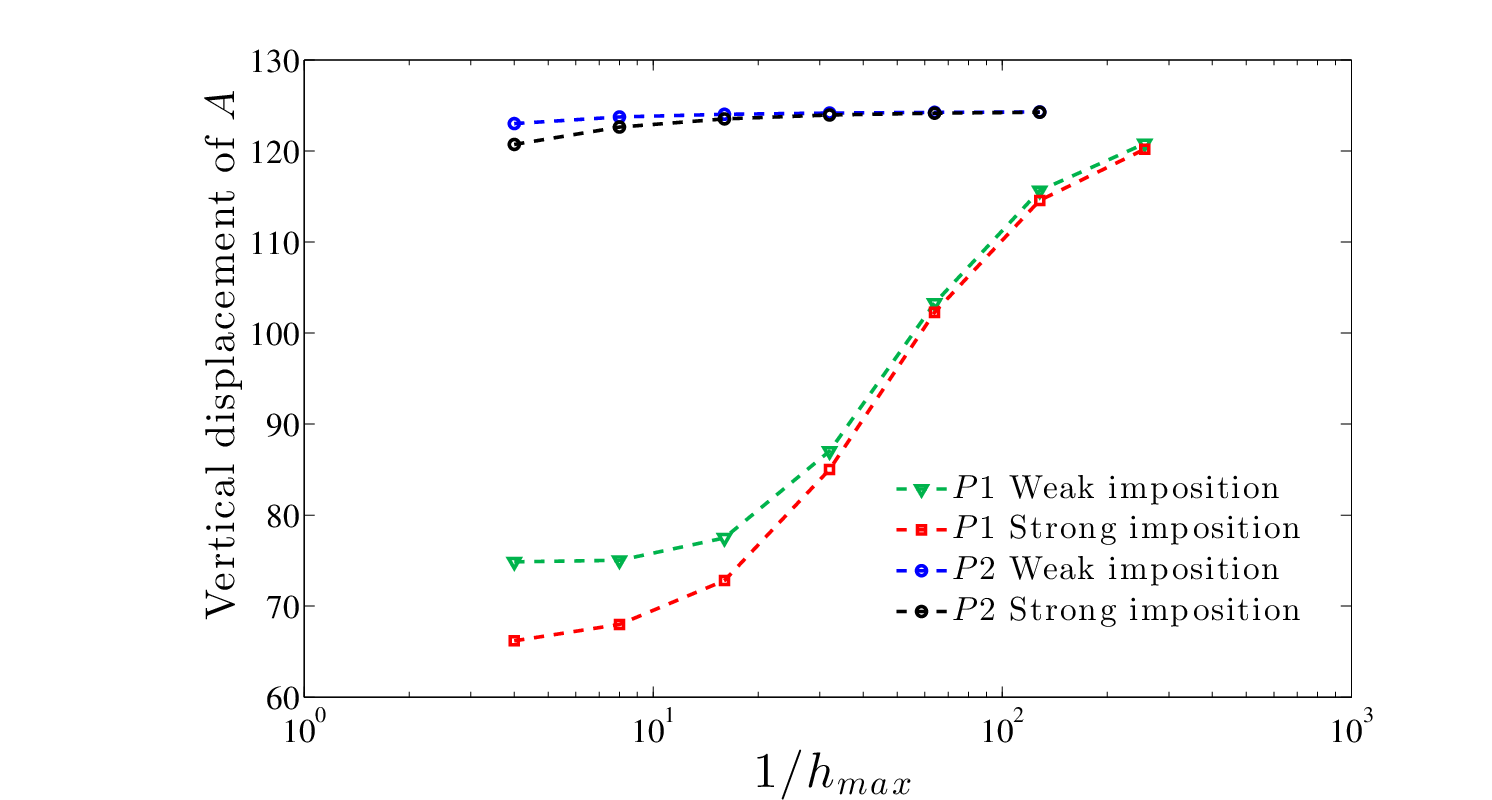
Refer to caption
Figure 9: Convergence of the vertical displacement, E=250E=250 ν=0.4999\nu=0.4999.

Figure 9 represents the vertical displacement of the point AA (top corner) versus the meshsize. We observe locking for both methods for first order approximation. The second order approximation converges without locking even for the coarse meshes. Similarly as the previous case the convergence is faster for the weak imposition. In view of the observed locking, we use the nearly incompressible problem to perform the same computations. The nearly incompressible problem, is obtained considering (2) and replacing ∇⋅\boldsymbol​u=0\nabla\cdot\boldsymbol{u}=0 by ∇⋅\boldsymbol​u=p/λ\nabla\cdot\boldsymbol{u}=p/\lambda.

Refer to caption
Figure 10: Convergence of the vertical displacement, E=250E=250 ν=0.4999\nu=0.4999.

Figure 10 displays the nearly incompressible elasticity for first and second order approximations for the weak and strong imposition but also the compressible elasticity with second order approximation. It shows that for nearly incompressible elasticity there is no locking for the method using first order polynomial approximation however for second order approximation the compressible elasticity converges faster than the nearly incompressible elasticity. Once again the weak imposition case converges faster than the strong imposition.

Appendix

Proof of Lemma 2.4

  • •
    \eqref

    stdapprox
    There exists x0∈Fjx_{0}\in F_{j} such that (\boldsymbol​uh−\boldsymbol​u¯hj)​(x0)=0(\boldsymbol{u}_{h}-\overline{\boldsymbol{u}}_{h}^{j})(x_{0})=0, then for x∈Fjx\in F_{j}

    (\boldsymboluh−\boldsymbol​u¯hj)(x)=∫x0x∇\boldsymboluh⋅\boldsymbolτ\textds,(\boldsymbol{u}_{h}-\overline{\boldsymbol{u}}_{h}^{j})(x)=\int_{x_{0}}^{x}\nabla\boldsymbol{u}_{h}\cdot\boldsymbol{\tau}~\text{d}s,

    using the Cauchy-Schwarz inequality it follows that

    ‖\boldsymboluh−\boldsymbol​u¯hj‖Fj\lesssim(∫Fj(∫Fj|∇\boldsymboluh⋅\boldsymbolτ|\textds)2\textds)12\lesssimh12‖∇\boldsymboluh⋅\boldsymbolτ‖Fj(∫Fj\textds)12.\left\|\boldsymbol{u}_{h}-\overline{\boldsymbol{u}}_{h}^{j}\right\|_{F_{j}}\lesssim\left(\int_{F_{j}}\left(\int_{F_{j}}\left|\nabla\boldsymbol{u}_{h}\cdot\boldsymbol{\tau}\right|~\text{d}s\right)^{2}\text{d}s\right)^{\frac{1}{2}}\lesssim h^{\frac{1}{2}}\left\|\nabla\boldsymbol{u}_{h}\cdot\boldsymbol{\tau}\right\|_{F_{j}}\left(\int_{F_{j}}\text{d}s\right)^{\frac{1}{2}}.
  • •
    \eqref

    inequality4
    The triangle inequality gives

    ‖h−12​\boldsymbol​uh‖Fj2≤‖h−12​(\boldsymbol​uh−\boldsymbol​u¯h)‖Fj2+‖h−12​\boldsymbol​u¯h‖Fj2,\left\|h^{-\frac{1}{2}}\boldsymbol{u}_{h}\right\|_{F_{j}}^{2}\leq\left\|h^{-\frac{1}{2}}\left(\boldsymbol{u}_{h}-\bar{\boldsymbol{u}}_{h}\right)\right\|_{F_{j}}^{2}+\left\|h^{-\frac{1}{2}}\bar{\boldsymbol{u}}_{h}\right\|_{F_{j}}^{2},

    considering the inequality (6) and the trace inequality we can write

    ‖(\boldsymboluh−\boldsymbol​u¯h)‖Fj\lesssimh12‖∇\boldsymboluh‖Pj.\left\|\left(\boldsymbol{u}_{h}-\bar{\boldsymbol{u}}_{h}\right)\right\|_{F_{j}}\lesssim h^{\frac{1}{2}}\left\|\nabla\boldsymbol{u}_{h}\right\|_{P_{j}}.
  • •
    \eqref

    inequality7
    Applying the Poincaré inequality, on each patch PjP_{j} the inequality follows.

  • •
    \eqref

    keyineq1, \eqrefkeyineq2
    Using the properties of \boldsymbol​vj\boldsymbol{v}_{j} \eqrefdefvgamma, \eqrefprop_vj and the Lemma 4.1 of Burman (2012).

Proof of Lemma 3.1

Proof 5.1.

In the rotated frame (ξ,η)(\xi,\eta), applying the definition of the P0P_{0}-projection, we can write the bilinear form as

⟨λ​∇^⋅\boldsymbol​v^j,\boldsymbol​u^h⋅\boldsymbol​n^⟩F^j\displaystyle\left\langle\lambda\hat{\nabla}\cdot\hat{\boldsymbol{v}}_{j},\hat{\boldsymbol{u}}_{h}\cdot\hat{\boldsymbol{n}}\right\rangle_{\hat{F}_{j}} =\displaystyle= λ​∫F^j(α1​∂v^1∂ξ+α2​∂v^2∂η)​u^2​\text​𝑑s^\displaystyle\lambda\int_{\hat{F}_{j}}\left(\alpha_{1}\frac{\partial\hat{v}_{1}}{\partial\xi}+\alpha_{2}\frac{\partial\hat{v}_{2}}{\partial\eta}\right)\hat{u}_{2}~\text{d}\hat{s}
=\displaystyle= λ​∫F^jα1​∂v^1∂ξ​u^2+α2​1h​(P0​u^2)2​\text​𝑑s^+λ​∫F^jα2​∂v^2∂η​(u^2−P0​u^2)​\text​𝑑s^.\displaystyle\lambda\int_{\hat{F}_{j}}\alpha_{1}\frac{\partial\hat{v}_{1}}{\partial\xi}\hat{u}_{2}+\alpha_{2}\frac{1}{h}\left(P_{0}\hat{u}_{2}\right)^{2}~\text{d}\hat{s}+\lambda\int_{\hat{F}_{j}}\alpha_{2}\frac{\partial\hat{v}_{2}}{\partial\eta}\left(\hat{u}_{2}-P_{0}\hat{u}_{2}\right)~\text{d}\hat{s}.

We observe that ∂v^1∂ξ=∇^⋅(v^1,0)T.\frac{\partial\hat{v}_{1}}{\partial\xi}=\hat{\nabla}\cdot(\hat{v}_{1},0)^{\rm T}. Using the trace inequality, the inverse inequality and \eqrefkeyineq1 \eqrefkeyineq2, we can show

‖∂v^1∂ξ‖F^j​\lesssim​h−1​‖\boldsymbol​u¯hj⋅\boldsymbol​τ‖Fj.\left\|\frac{\partial\hat{v}_{1}}{\partial\xi}\right\|_{\hat{F}_{j}}\lesssim h^{-1}\left\|\overline{\boldsymbol{u}}_{h}^{j}\cdot\boldsymbol{\tau}\right\|_{F_{j}}.

Note that ∫F^j∂v^1∂ξ​\text​𝑑s^=0\int_{\hat{F}_{j}}\frac{\partial\hat{v}_{1}}{\partial\xi}~\text{d}\hat{s}=0, using these properties and the inequality (6), it follows that

λ​∫F^jα1​∂v^1∂ξ​u^2​\text​𝑑s^\displaystyle\lambda\int_{\hat{F}_{j}}\alpha_{1}\frac{\partial\hat{v}_{1}}{\partial\xi}\hat{u}_{2}~\text{d}\hat{s} =\displaystyle= λ​∫F^jα1​∂v^1∂ξ​(u^2−P0​u^2)​\text​𝑑s^\displaystyle\lambda\int_{\hat{F}_{j}}\alpha_{1}\frac{\partial\hat{v}_{1}}{\partial\xi}\left(\hat{u}_{2}-P_{0}\hat{u}_{2}\right)~\text{d}\hat{s}
≥\displaystyle\geq −C​α1​h−1​‖λ12​\boldsymbol​u¯hj⋅\boldsymbol​τ‖Fj​‖λ12​(\boldsymbol​uh−\boldsymbol​u¯hj)⋅\boldsymbol​n‖Fj\displaystyle-C\alpha_{1}h^{-1}\left\|\lambda^{\frac{1}{2}}\overline{\boldsymbol{u}}_{h}^{j}\cdot\boldsymbol{\tau}\right\|_{F_{j}}\left\|\lambda^{\frac{1}{2}}\left(\boldsymbol{u}_{h}-\overline{\boldsymbol{u}}_{h}^{j}\right)\cdot\boldsymbol{n}\right\|_{F_{j}}
≥\displaystyle\geq −C​α124​ϵ‖λ12h12\boldsymbol​u¯hj⋅\boldsymbolτ‖Fj2−ϵ‖λ12∇\boldsymboluh‖Pj2.\displaystyle-\frac{C\alpha_{1}^{2}}{4\epsilon}\left\|\frac{\lambda^{\frac{1}{2}}}{h^{\frac{1}{2}}}\overline{\boldsymbol{u}}_{h}^{j}\cdot\boldsymbol{\tau}\right\|_{F_{j}}^{2}-\epsilon\left\|\lambda^{\frac{1}{2}}\nabla\boldsymbol{u}_{h}\right\|_{P_{j}}^{2}.

Using (3) we can obtain similarly

λ​∫F^jα2​∂v^2∂η​(u^2−P0​u^2)​\text​𝑑s^\displaystyle\lambda\int_{\hat{F}_{j}}\alpha_{2}\frac{\partial\hat{v}_{2}}{\partial\eta}\left(\hat{u}_{2}-P_{0}\hat{u}_{2}\right)~\text{d}\hat{s} ≥\displaystyle\geq −C​α224​ϵ‖λ12h12\boldsymbol​u¯hj⋅\boldsymboln‖Fj2−ϵ‖λ12∇\boldsymboluh‖Pj2,\displaystyle-\frac{C\alpha_{2}^{2}}{4\epsilon}\left\|\frac{\lambda^{\frac{1}{2}}}{h^{\frac{1}{2}}}\overline{\boldsymbol{u}}_{h}^{j}\cdot\boldsymbol{n}\right\|_{F_{j}}^{2}-\epsilon\left\|\lambda^{\frac{1}{2}}\nabla\boldsymbol{u}_{h}\right\|_{P_{j}}^{2},
λ​∫F^jα2​1h​(P0​u^2)2​\text​𝑑s^\displaystyle\lambda\int_{\hat{F}_{j}}\alpha_{2}\frac{1}{h}\left(P_{0}\hat{u}_{2}\right)^{2}~\text{d}\hat{s} =\displaystyle= α2​‖λ12h12​\boldsymbol​u¯hj⋅\boldsymbol​n‖Fj2.\displaystyle\alpha_{2}\left\|\frac{\lambda^{\frac{1}{2}}}{h^{\frac{1}{2}}}\overline{\boldsymbol{u}}_{h}^{j}\cdot\boldsymbol{n}\right\|_{F_{j}}^{2}.

Proof of Lemma 3.2

Proof 5.2.

In the rotated frame (ξ,η)(\xi,\eta), applying the definition of the P0P_{0}-projection, we can write the bilinear form similarly as in the previous proof

⟨2​μ​\boldsymbol​ε^​(\boldsymbol​v^j)⋅\boldsymbol​n^,\boldsymbol​u^h⟩F^j\displaystyle\left\langle 2\mu\hat{\boldsymbol{\varepsilon}}\left(\hat{\boldsymbol{v}}_{j}\right)\cdot\hat{\boldsymbol{n}},\hat{\boldsymbol{u}}_{h}\right\rangle_{\hat{F}_{j}} =\displaystyle= μ​∫F^jα1​∂v^1∂η​u^1+α2​∂v^2∂ξ​u^1+2​α2​∂v^2∂η​u^2​\text​𝑑s^\displaystyle\mu\int_{\hat{F}_{j}}\alpha_{1}\frac{\partial\hat{v}_{1}}{\partial\eta}\hat{u}_{1}+\alpha_{2}\frac{\partial\hat{v}_{2}}{\partial\xi}\hat{u}_{1}+2\alpha_{2}\frac{\partial\hat{v}_{2}}{\partial\eta}\hat{u}_{2}~\text{d}\hat{s}
=\displaystyle= μ​∫F^jα1​1h​(P0​u^1)2+α2​∂v^2∂ξ​u^1+α2​2h​(P0​u^2)2​\text​𝑑s^\displaystyle\mu\int_{\hat{F}_{j}}\alpha_{1}\frac{1}{h}\left(P_{0}\hat{u}_{1}\right)^{2}+\alpha_{2}\frac{\partial\hat{v}_{2}}{\partial\xi}\hat{u}_{1}+\alpha_{2}\frac{2}{h}\left(P_{0}\hat{u}_{2}\right)^{2}~\text{d}\hat{s}
+μ∫F^jα1∂v^1∂η(u^1−P0u^1)\textds^+2μ∫F^jα2∂v^2∂η(u^2−P0u^2)\textds^.\displaystyle+\mu\int_{\hat{F}_{j}}\alpha_{1}\frac{\partial\hat{v}_{1}}{\partial\eta}\left(\hat{u}_{1}-P_{0}\hat{u}_{1}\right)~\text{d}\hat{s}+2\mu\int_{\hat{F}_{j}}\alpha_{2}\frac{\partial\hat{v}_{2}}{\partial\eta}\left(\hat{u}_{2}-P_{0}\hat{u}_{2}\right)~\text{d}\hat{s}.

Term by term we obtain

μ​∫F^jα1​1h​(P0​u^1)2​\text​𝑑s^\displaystyle\mu\int_{\hat{F}_{j}}\alpha_{1}\frac{1}{h}\left(P_{0}\hat{u}_{1}\right)^{2}~\text{d}\hat{s} =\displaystyle= α1​‖μ12h12​\boldsymbol​u¯hj⋅\boldsymbol​τ‖Fj2,\displaystyle\alpha_{1}\left\|\frac{\mu^{\frac{1}{2}}}{h^{\frac{1}{2}}}\overline{\boldsymbol{u}}_{h}^{j}\cdot\boldsymbol{\tau}\right\|_{F_{j}}^{2},
μ​∫F^jα2​2h​(P0​u^2)2​\text​𝑑s^\displaystyle\mu\int_{\hat{F}_{j}}\alpha_{2}\frac{2}{h}\left(P_{0}\hat{u}_{2}\right)^{2}~\text{d}\hat{s} =\displaystyle= 2​α2​‖μ12h12​\boldsymbol​u¯hj⋅\boldsymbol​n‖Fj2,\displaystyle 2\alpha_{2}\left\|\frac{\mu^{\frac{1}{2}}}{h^{\frac{1}{2}}}\overline{\boldsymbol{u}}_{h}^{j}\cdot\boldsymbol{n}\right\|_{F_{j}}^{2},
μ​∫F^jα1​∂v^1∂η​(u^1−P0​u^1)​\text​𝑑s^\displaystyle\mu\int_{\hat{F}_{j}}\alpha_{1}\frac{\partial\hat{v}_{1}}{\partial\eta}\left(\hat{u}_{1}-P_{0}\hat{u}_{1}\right)~\text{d}\hat{s} ≥\displaystyle\geq −C​α124​ϵ‖μ12h12\boldsymbol​u¯hj⋅\boldsymbolτ‖Fj2−ϵ‖μ12∇\boldsymboluh‖Pj2,\displaystyle-\frac{C\alpha_{1}^{2}}{4\epsilon}\left\|\frac{\mu^{\frac{1}{2}}}{h^{\frac{1}{2}}}\overline{\boldsymbol{u}}_{h}^{j}\cdot\boldsymbol{\tau}\right\|_{F_{j}}^{2}-\epsilon\left\|\mu^{\frac{1}{2}}\nabla\boldsymbol{u}_{h}\right\|_{P_{j}}^{2},
2​μ​∫F^jα2​∂v^2∂η​(u^2−P0​u^2)​\text​𝑑s^\displaystyle 2\mu\int_{\hat{F}_{j}}\alpha_{2}\frac{\partial\hat{v}_{2}}{\partial\eta}\left(\hat{u}_{2}-P_{0}\hat{u}_{2}\right)~\text{d}\hat{s} ≥\displaystyle\geq −C​α22ϵ‖μ12h12\boldsymbol​u¯hj⋅\boldsymboln‖Fj2−ϵ‖μ12∇\boldsymboluh‖Pj2.\displaystyle-\frac{C\alpha_{2}^{2}}{\epsilon}\left\|\frac{\mu^{\frac{1}{2}}}{h^{\frac{1}{2}}}\overline{\boldsymbol{u}}_{h}^{j}\cdot\boldsymbol{n}\right\|_{F_{j}}^{2}-\epsilon\left\|\mu^{\frac{1}{2}}\nabla\boldsymbol{u}_{h}\right\|_{P_{j}}^{2}.

We observe that ∂v^2∂ξ=∇^​(0,v^2)T⋅\boldsymbol​τ.\frac{\partial\hat{v}_{2}}{\partial\xi}=\hat{\nabla}(0,\hat{v}_{2})^{\rm T}\cdot\boldsymbol{\tau}. Using the trace inequality, the inverse inequality and \eqrefkeyineq1 \eqrefkeyineq2, we can show

‖∂v^2∂ξ‖F^j​\lesssim​h−1​‖\boldsymbol​u¯hj⋅\boldsymbol​n‖Fj.\left\|\frac{\partial\hat{v}_{2}}{\partial\xi}\right\|_{\hat{F}_{j}}\lesssim h^{-1}\left\|\overline{\boldsymbol{u}}_{h}^{j}\cdot\boldsymbol{n}\right\|_{F_{j}}.

Note that since ∫F^j∂v^2∂ξ​\text​𝑑s^=0\int_{\hat{F}_{j}}\frac{\partial\hat{v}_{2}}{\partial\xi}~\text{d}\hat{s}=0, we obtain

μ∫F^jα2∂v^2∂ξu^1\textds^=μ∫F^jα2∂v^2∂ξ(u^1−P0u^1)\textds^≥−C​α224​ϵ‖μ12h12\boldsymbol​u¯hj⋅\boldsymboln‖Fj2−ϵ‖μ12∇\boldsymboluh‖Pj2.\mu\int_{\hat{F}_{j}}\alpha_{2}\frac{\partial\hat{v}_{2}}{\partial\xi}\hat{u}_{1}~\text{d}\hat{s}=\mu\int_{\hat{F}_{j}}\alpha_{2}\frac{\partial\hat{v}_{2}}{\partial\xi}\left(\hat{u}_{1}-P_{0}\hat{u}_{1}\right)~\text{d}\hat{s}\geq-\frac{C\alpha_{2}^{2}}{4\epsilon}\left\|\frac{\mu^{\frac{1}{2}}}{h^{\frac{1}{2}}}\overline{\boldsymbol{u}}_{h}^{j}\cdot\boldsymbol{n}\right\|_{F_{j}}^{2}-\epsilon\left\|\mu^{\frac{1}{2}}\nabla\boldsymbol{u}_{h}\right\|_{P_{j}}^{2}.

Acknowledgement

This work received funding from EPSRC (award number EP/J002313/1) which is gratefully acknowledged. We also thank an anonymous reviewer for suggesting the study of the Cook’s membrane.

References

  • Brenner & Scott (2008) Brenner, S. C. & Scott, L. R. (2008) The mathematical theory of finite element methods. Texts in Applied Mathematics, vol. 15, third edn. New York: Springer, pp. xviii+397.
  • Burman (2012) Burman, E. (2012) A penalty free nonsymmetric Nitsche-type method for the weak imposition of boundary conditions. SIAM J. Numer. Anal., 50, 1959–1981.
  • Burman & Fernández (2014) Burman, E. & Fernández, M. A. (2014) Explicit strategies for incompressible fluid-structure interaction problems: Nitsche type mortaring versus Robin–Robin coupling. International Journal for Numerical Methods in Engineering, 97, 739–758.
  • Burman & Stamm (2010) Burman, E. & Stamm, B. (2010) Bubble stabilized discontinuous Galerkin method for parabolic and elliptic problems. Numerische Mathematik, 116, 213–241.
  • Freund & Stenberg (1995) Freund, J. & Stenberg, R. (1995) On weakly imposed boundary conditions for second order problems. Proceedings of the International Conference on Finite Element in Fluids - New trends and applications.
  • Girault & Raviart (1986) Girault, V. & Raviart, P. (1986) Finite element methods for Navier-Stokes equations: theory and algorithms. Springer series in computational mathematics. Springer-Verlag.
  • Girault & Rivière (2009) Girault, V. & Rivière, B. (2009) DG Approximation of Coupled Navier–Stokes and Darcy Equations by Beaver–Joseph–Saffman Interface Condition. SIAM Journal on Numerical Analysis, 47, 2052–2089.
  • Hecht (2012) Hecht, F. (2012) New development in freefem++. J. Numer. Math., 20, 251–265.
  • Hughes et al. (2000) Hughes, T. J. R., Engel, G., Mazzei, L. & Larson, M. G. (2000) A comparison of discontinuous and continuous Galerkin methods based on error estimates, conservation, robustness and efficiency. Discontinuous Galerkin methods (Newport, RI, 1999). Lect. Notes Comput. Sci. Eng., vol. 11. Berlin: Springer, pp. 135–146.
  • Larson & Niklasson (2004) Larson, M. & Niklasson, A. (2004) Analysis of a nonsymmetric discontinuous Galerkin method for elliptic problems: stability and energy error estimates. SIAM Journal on Numerical Analysis, 42, 252–264.
  • Lax (2002) Lax, P. D. (2002) Functional analysis. Pure and Applied Mathematics (New York). Wiley-Interscience [John Wiley & Sons], New York, pp. xx+580.
  • Nitsche (1971) Nitsche, J. (1971) Über ein variationsprinzip zur lösung von Dirichlet-problemen bei verwendung von teilräumen, die keinen randbedingungen unterworfen sind. Abhandlungen aus dem Mathematischen Seminar der Universität Hamburg, 36, 9–15.
  • Oden et al. (1998) Oden, J. T., Babuŝka, I. & Baumann, C. E. (1998) A discontinuous hp finite element method for diffusion problems. Journal of Computational Physics, 146, 491 – 519.
  • Scott & Zhang (1990) Scott, L. R. & Zhang, S. (1990) Finite element interpolation of nonsmooth functions satisfying boundary conditions. Math. Comp., 54, 483–493.