Anisotropy of the superconducting fluctuations in multiband superconductors:
the case of LiFeAs

After the original discovery of superconductivity in LaOFeAs[1] the investigation of iron-based superconductors has lead to the discovery of several classes of compounds that all display a high-temperature superconductivity, despite the fact that the different lattice structures can lead to significant differences in the electronic properties[2, 3]. Such differences justify the on-going debate on the existence of an universal pairing mechanism in all iron-based superconductors. One of the crucial questions concerns the role of antiferromagnetic spin fluctuations. Indeed, while they represent a plausible candidate for the pairing glue in those systems, as 122 compounds, with good nesting conditions between the hole and electron Fermi pockets[3, 4, 5], their relevance in other systems with poor nesting properties is often questioned[7, 8, 6, 9]. A typical example of such a system is LiFeAs. This compound is a stochiometric superconductor with a $T_{c}\sim 17$ K[10] and no magnetic ordering. Due to its stochiometric nature and its clean, charge neutral cleaved surface LiFeAs is the best candidate to perform both bulk- and surface-sensitive measurements. However, the large amount of experimental findings accumulated so far did not succeeded yet to clarify the nature of the pairing mechanism, but offered instead a puzzling and somehow contradictory scenario. The Fermi surface (FS) of LiFeAs observed by angle-resolved photoemission spectroscopy (ARPES) consists of two hole pockets at $\Gamma$ and two electron pockets at $M$[11, 12, 13], as in all pnictides families. However, there are some remarkable quantitative differences, which are only partly accounted for by LDA+DMFT (Dynamical Mean Field Theory) calculations[15, 14]. In particular, the FS nesting is relatively poor and the hole pockets are much shallower than in other families, with associated larger density of states (DOS) which has been suggested to promote ferromagnetic fluctuations instead of the antiferromagnetic ones[8]. Nonetheless, as stressed by several authors, despite the poor nesting, a spin-fluctuation mediated pairing[18, 14, 19, 20], or more generically a strong interband nature of the interaction[21], cannot be excluded. Indeed, while perfect nesting is required to have a long-ranged SDW instability (absent in LiFeAs), the presence of large spin fluctuations is sufficient to justify a spin-mediated pairing mechanism, leading to a $s^{\pm}$ order parameter. Such large magnetic fluctuations in LiFeAs have been observed by nuclear magnetic resonance[22] and neutron scattering experiments[16, 17], that also identified a magnetic vector slightly incommensurate[17] with respect to the ${\bf Q}=(\pi,\pi)$ wavevector, due probably to the bad nesting condition of the FS. While these finding can support a $s^{\pm}$ scenario, its agreement with the ARPES data on the gap modulation is still under scrutiny[12, 23, 24]. Also the quasiparticle interference patterns observed in scanning tunneling microscopy[25, 26, 27] are subject of an intense debate. In this case different assumptions on the impurity scattering mechanism can make the experimental results compatible either with a $s^{\pm}$[25] or with a (triplet) $p$-wave[26, 27] symmetry of the order parameter.

The anomalies of LiFeAs are not restricted to the superconducting (SC) state but extend up to the so called normal state. The phenomenology and in particular the dimensionality of SC fluctuations above $T_{c}$ is an highly debated issue for all pnictides[28]. However the situation in LiFeAs is particularly puzzling. Indeed, while electronic properties of LiFeAs are believed to have an almost three-dimensional (3D) character[15], as confirmed by de Haas van Alphen experiments[29, 30], the superconducting fluctuations (SCF) exhibit a marked two-dimensional (2D) fluctuation regime, which extends up to temperatures very near to $T_{c}$[31, 32]. At the same time, the measurements of the upper critical field[33] slight below $T_{c}$ would point instead to a small anisotropy between in-plane and out-of-plane SCF, at odd with paraconductivity results. As we discuss in the present manuscript, the apparent contradictions between these results can be reconciled by taking into account both the multiband structure of pnictides and the peculiar interband character of the interactions. In particular, in multiband systems the link between the band structure and the nature of SCF, both above and below $T_{c}$, can be more involved than what expected in the single-band case, as pointed out in different contexts in the recent literature.[34, 35, 36, 37] At the same time the interband character of the pairing can lead to remarkable qualitative differences with respect to single-band systems, as it has been emphasized in the context of transport[38] and optical properties above $T_{c}$[39]. In the present work we analyze the SCF above $T_{c}$ in LiFeAs by taking the point of view of a spin-mediated interband pairing mechanism, whose properties can be deduced by the analysis of the SCF themselves. We show that the microscopic estimate of the crossover temperature from 2D to 3D regime for the SCF is controlled by three cooperative mechanisms: (i) the interband nature of the pairing, which leads to a weighted contribution of the various bands in the single collective mode which controls the critical SCF[34]; (ii) the low-energy renormalization effects beyond Density Functional Theory (DFT), due the exchange of spin fluctuations[39]; (iii) the anisotropy of the pairing, that can make the SCF quasi-2D even for quasi-3D band dispersions. On this respect our work supports recent theoretical attempts [19, 21] to reproduce the measured gap hierarchy by taking into account the possible variations of the pairing interaction along $z$, due to the evolution of the FS. Our main finding is that the marked 2D character of SCF points towards a prevalent 2D nature of the spin-fluctuation mediated pairing interaction, that seems consistent with experimental observation of the magnetic fluctuations above $T_{c}$[22, 31]. Such a result is not inconsistent with other estimates of the SC-properties anisotropy done below $T_{c}$ with different probes, as the upper critical field[33], the thermal conductivity[40] and the critical current[41]. Indeed, as we discuss below, in a multiband superconductor the weight of the various bands to the SCF depends on the quantity under scrutiny, leading to different results in the various experimental set-up. Finally, while our findings cannot exclude an alternative pairing scenario based either on ferromagnetic[8] or orbital[9] fluctuations, the predominant intraband character of these mechanisms seems more difficult to reconcile with an anisotropic pairing mechanism, crucial to interpret the SCF above $T_{c}$.

Let us first of all summarize the expected result for the SCF anisotropy on the basis of the derivation of Ref. [34], that was done under the following hypotheses: (i) the interaction has a predominant interband character and (ii) the pairing is isotropic in momentum space (so it has the same strength at all $k_{z}$ values). In this situation, it has been demonstrated that despite the presence of multiple FS the effective action of the SCF is still characterized by the emergence of a single critical collective mode that in the case of a layered superconductor is described by the propagator:

$$L^{-1}({\bf q},\omega_{m})=\nu\left[\epsilon+\eta_{\parallel}q_{\parallel}^{2}+r_{z}\sin(q_{z}d/2)+\gamma|\omega_{m}|\right]$$

(1)

where $\nu$ is the effective DOS of the collective mode at the Fermi level, $\eta_{\parallel}$ and $r_{z}$ are the in-plane and the out-of-plane stiffness respectively, $\varepsilon=\ln(T/T_{c})$ and we used a periodic notation for the $q_{z}$ dispersion, with $d$ interlayer spacing. As a consequence the resulting expression for the paraconductivity is the same obtained for a single-band layered superconductor[42], i.e.

$$\delta\sigma=\frac{e^{2}}{16\hbar d\sqrt{\varepsilon(\varepsilon+r_{z})}}.$$

(2)

The crossover from 2D behavior $\delta\sigma\sim 1/{\varepsilon}$ to 3D one $\delta\sigma\sim 1/\sqrt{\varepsilon}$ occurs at the temperature where $\varepsilon\lesssim r_{z}$. In LiFeAs the 2D behavior is preserved until $\epsilon\sim 0.02$, so that one deduces that the out-of-plane stiffness $r_{z}$ is very small. In the single-band case the in-plane $\eta$ and out-of-plane $r_{z}$ stiffness can be estimated microscopically from the values of the in-plane velocity and out-of-plane hopping[42]:

$$\eta\sim\frac{v_{F}^{2}}{T^{2}},\quad r_{z}\sim\frac{t_{z}^{2}}{T^{2}}.$$

(3)

In the multiband case the contribution of each band to the critical-mode values for $\eta_{\parallel}$ and $r_{z}$ depends in general on the relative strength of intra- vs inter-band pairing[43, 34]. However, in the case of pnictides the assumption of a predominant interband coupling simplifies considerably the description of the critical collective mode. Following Ref. [34] we shall consider a four-band model with only interband pairing. By taking into account DFT calculations[15] and ARPES evidences[11, 12] for LiFeAs we will consider two electronic $\gamma_{1},\gamma_{2}$ bands degenerate, and two hole bands $\alpha$ and $\beta$, corresponding to the inner and outer hole pockets, respectively. The larger coupling $\lambda$ occurs between the quasi-nested $\alpha$ and $\gamma_{i}$ bands, while the $\beta-\gamma$ coupling $\lambda_{\beta\gamma}=\kappa\lambda$, $\kappa<1$ is assumed to be smaller due to the larger size of the $\beta$ pocket. The BCS-like Hamiltonian of the model is

$$H=\sum_{i}H_{0}^{i}+\lambda\sum_{\bf q}\left[\Phi^{\dagger}_{\gamma,{\bf q}}(\Phi^{\phantom{\dagger}}_{\alpha,{\bf q}}+\kappa\Phi^{\phantom{\dagger}}_{\beta,{\bf q}})+h.c.\right].$$

(4)

Here $H_{0}^{i}=\sum_{\bf k}\xi^{i}_{{\bf k}}c^{\dagger}_{i,{\bf k}\sigma}c^{\phantom{\dagger}}_{i,{\bf k}\sigma}$, $c_{i,{\bf k}\sigma}^{(\dagger)}$ annihilates (creates) a fermion in the $i=\alpha,\beta,\gamma_{1},\gamma_{2}$ band and $\xi^{i}_{{\bf k}}$ is the layered 3D band dispersion with respect to the chemical potential

$$\xi^{i}_{{\bf k}}=\frac{{\bf k}_{\parallel}^{2}}{2m_{i}}-t_{i,z}\cos(k_{z}d)-\mu.$$

(5)

In Eq. (4) $\Phi_{i,{\bf q}}=\sum_{\bf k}c^{\phantom{\dagger}}_{i,{\bf k}+{\bf q}\uparrow}c^{\phantom{\dagger}}_{i,{\bf k}\downarrow}$ is the pairing operator in the $i$-th band, with $\Phi_{\gamma,{\bf q}}\equiv\Phi_{\gamma_{1},{\bf q}}+\Phi_{\gamma_{2},{\bf q}}$. It is possible to recast the four-band model defined in Eq. (4) in an effective two-band model by introducing the pairing operators $\Phi_{e}\equiv\Phi_{\gamma}$ and $\Phi_{h}\equiv\Phi_{\alpha}+\kappa\Phi_{\beta}$ so that the pairing term reads:

$$H_{I}=\lambda\sum_{\bf q}(\Phi_{1}^{\dagger}\Phi_{2}^{\phantom{\dagger}}+h.c.).$$

(6)

Once established the pairing model according to Eq. (6), we will use band parameters consistent with LDA+DMFT and experimental measurements,[15, 14, 12, 11] and we will choose the interaction strength in order to reproduce the experimental gap values. The estimate of the fluctuation regime will then follow by the explicit calculation of the critical multiband mode, done according to the analysis of Ref. [34]. Notice that despite the repulsive nature of the interaction (6) a superconducting instability is still possible in the $s_{\pm}$ symmetry, where the gap changes sign between hole and electron bands. However, in contrast to the ordinary intraband-dominated pairing (as, e.g., in MgB₂[43]) here a single pairing channel exists, with important consequences on the implementation of the standard procedure to derive the effective action for the SC fluctuations both above[34] and below [37] $T_{c}$. In particular, one can show that in the model (4)-(6) the contribution of the various bands to the single critical mode (1) is given by:

$$\eta_{\parallel}=(w_{h}^{2}\eta_{h}+w_{e}^{2}\eta_{e}),\quad r_{z}=(w_{h}^{2}r_{h}+w_{e}^{2}r_{e})$$

(7)

where the coefficients $w_{e}$, $w_{h}$ are fixed by the two conditions:

	$\displaystyle w_{e}w_{h}$	$\displaystyle=$	$\displaystyle 1,$		(8)
	$\displaystyle\frac{w_{e}^{2}}{w_{h}^{2}}$	$\displaystyle=$	$\displaystyle\frac{\Delta^{2}_{e}}{\Delta^{2}_{h}}=\frac{\Pi_{h}(q=0)}{\Pi_{e}(q=0)},$		(9)

where $\Pi_{h}\equiv\Pi_{\alpha}+\kappa^{2}\Pi_{\beta},\Pi_{e}=2\Pi_{\gamma_{1}}$ are the Cooper particle-particle bubbles evaluated at zero frequency and momentum ($q=(i\omega_{n},{\bf q})$), $\Delta_{h}\equiv\Delta_{\alpha}=\Delta_{\beta}/\kappa$ and $\Delta_{e}\equiv\Delta_{\gamma_{i}}$. The last relation of Eq. (9) has been derived from the usual saddle-point equations $\Delta_{e}=-\lambda\Pi_{h}\Delta_{h}$ and $\Delta_{h}=-\lambda\Pi_{e}\Delta_{e}$. Analogously, the SCF parameters $\eta_{e(h)}$, $r_{e(h)}$, which are obtained by the small ${\bf q}$ expansion of the Cooper bubbles (see below), are given in term of the band stiffnesses as

	$\displaystyle\eta_{e}$	$\displaystyle=$	$\displaystyle 2\eta_{\gamma},\quad\quad\eta_{h}=\eta_{\alpha}+\kappa^{2}\eta_{\beta},$		(10)
	$\displaystyle r_{e}$	$\displaystyle=$	$\displaystyle 2r_{\gamma},\quad\quad r_{h}=r_{\alpha}+\kappa^{2}r_{\beta},$		(11)

In first approximation the coefficients $\eta_{i}$ and $r_{i}$ can be extracted from the band parameters, listed in Table I, according to Eq. (3). For what concerns the relative weights $w_{e,h}$ in Eq. (7) one can extend the relation (9) above $T_{c}$ where $\Pi_{i}\simeq\nu_{i}ln(\omega_{0}/T_{c})$, i.e. each band is weighted inversely proportional to its DOS $\nu_{i}$. By means of Eqs. (7), (9) and (11), and by using the band parameters listed in Table 1, extracted from LDA+DMFT and experimental measurements,[15, 14, 12, 11] we can provide a preliminary estimate of the anisotropy parameter $r_{z}$ for LiFeAs. As one can see in Table 1, even though the outer hole band has $t_{z}\approx 0$, the $t_{z}$ in the inner hole band and in the electron ones is quite larger, of order of $15$ meV. As a consequence from Eq.(3) one expects a value $r_{z}\sim{\cal O}(10)$ even considering the weighting factors $w_{e},w_{h}$ defined in Eq. (7) to compute the average $r_{z}$ of the critical collective mode. Such an estimate can be hardly reconciled with the experimental observation of a 2D regime for the SCF up to very small $\varepsilon\sim 0.02$, that would imply $r_{z}\sim 10^{-2}$.

All the above discussion has been based on the idea that the anisotropy of SCF is simply determined by the anisotropy of the band structure, and band parameters have been extracted from LDA+DMFT and ARPES measurements. In this Section we discuss how this estimate can be modified by taking into account several properties peculiar to pnictides. A first correction to be considered is the low-energy band renormalization due to the same spin fluctuations that mediate the pairing. Indeed, while LDA+DMFT correctly accounts for the high-energy effects (like Hubbard-$U$ interactions) that renormalize the overall bandwidth, spin fluctuations can give rise to an additional band renormalization visible in a small energy range (of the order of the spin-fluctuation scale $\omega_{0}\sim 10-20$ meV) around the Fermi level. The dichotomy between these two effects has been discussed for example in Ref. [39], where it has been show how these low-energy renormalization effects are crucial to understand the discrepancy between the effective masses probed by ARPES and the thermodynamical probes, sensible to the carrier mass at the Fermi level. By using the results of an Eliashberg-like approach to the spin-mediated interactions one can then introduce an additional reduction of the hopping parameters listed in Table I as $t_{i}\rightarrow t_{i}/(1+\lambda)$, where $\lambda$ represents here an average dimensionless coupling to spin fluctuations, estimated[39] to be in the intermediate-coupling regime $\lambda\sim 1-2$. By including this effect we already reduce $r_{z}$ to $\simeq 2$, that is however still much larger than the experimental value. A second aspect to be considered is the modulation of the pairing interaction along $k_{z}$. Indeed, it is well known that in the case of pnictides the structure of the pairing interaction along $k_{z}$ can be definitively much more involved, as it has been recently pointed out in the case of P-doped BaFeAs [45]. By assuming that the pairing originates mainly from a spin-fluctuations mediated interband mechanism, one must consider the evolution along the $z$ direction both of the orbital character of the bands and of the nesting properties between the (anisotropic) hole and electron pockets, that contribute both to the effective $k_{z}$ dependence of the pairing interaction. Both properties can vary between different materials and also as a function of doping. For example, in Co-doped BaFeAs it has been experimentally shown that spin fluctuations that are 3D anisotropic in the undoped compound become much more 2D in the optimally-doped one, where a 2D picture seems then more appropriate[46]. Even though a detailed experimental investigation of this issue on LiFeAs is not yet available, there have been already suggestions[19, 21] for a possible $k_{z}$ dependence of the pairing interactions induced by the variations of the FS topology along $z$. We analyze here the consequences on a anisotropic pairing interaction along $k_{z}$ for the properties of the SCF. In this case, while the structure (1) of the critical collective mode does not change, we must reconsider the estimate (3) of the single-band parameters when the pairing has an anisotropic structure along $k_{z}$. On very general grounds[42, 43, 34] the SCF stiffnesses $\eta_{i},r_{i}$ are extracted from the small ${\bf q}$ expansion of the Cooper bubbles in each band. If one introduces explicitly a modulation function $w(k_{z})$, that accounts for the variation of the pairing interaction along the $z$-axis, the Cooper bubble is:

	$\displaystyle\Pi_{i}({\bf q},0)$	$\displaystyle=$	$\displaystyle\frac{T}{N}\sum_{{\bf k},i\omega_{n}}w^{2}(k_{z})G_{i}({\bf k}+{\bf q},\omega_{n})G_{i}(-{\bf k},-\omega_{n})=$		(12)
		$\displaystyle=$	$\displaystyle\frac{1}{N}\sum_{\bf k}w^{2}(k_{z})\frac{f(-\xi^{i}_{\bf k})-f(\xi^{i}_{{\bf k}+{\bf q}})}{\xi^{i}_{\bf k}+\xi^{i}_{{\bf k}+{\bf q}}},$

where $G_{i}$ is the Green’s function of the $i$-th band above $T_{c}$. By retaining leading terms in the ${\bf q}^{2}$ expansion on Eq. (12) one obtains:

	$\displaystyle\nu_{i}\eta_{i}$	$\displaystyle=$	$\displaystyle\frac{1}{8N}\sum_{{\bf k}}w^{2}(k_{z})v^{2}_{i,\parallel}({\bf k})\Bigg[\frac{f^{\prime}(\xi^{i}_{\bf k})}{(\xi^{i}_{\bf k})^{2}}+\frac{\tanh{(\beta\xi^{i}_{\bf k}/2)}}{2(\xi^{i}_{\bf k})^{3}}\Bigg],$
	$\displaystyle\nu_{i}r_{i}$	$\displaystyle=$	$\displaystyle\frac{1}{4N}\sum_{{\bf k}}w^{2}(k_{z})v^{2}_{i,z}({\bf k})\Bigg[\frac{f^{\prime}(\xi^{i}_{\bf k})}{(\xi^{i}_{\bf k})^{2}}+\frac{\tanh{(\beta\xi^{i}_{\bf k}/2)}}{2(\xi_{\bf k}^{i})^{3}}\Bigg],$

where ${\bf v}_{\bf k}=\partial\xi_{\bf k}/\partial{\bf k}$, so that for a band dispersion as in Eq. (5) $v_{\parallel}({\bf k})=\partial_{{\bf k}_{\parallel}}\xi_{{\bf k}}$ and $v_{z}\sim\sin k_{z}$. The ${\bf k}$-integrals in Eqs. (III)-() are dominated by ${\bf k}=({\bf k}_{\parallel},k_{z})$ values at the FS. In particular for $w^{2}(k_{z})=1$ one recovers the usual estimates (3), so that $r_{z}$ scales as $t_{z}$. However, when $w^{2}(k_{z})$ is peaked at small $k_{z}$ values, where $v_{z}\sim 0$, and it is reduced at intermediate $k_{z}d\simeq\pi/2$, where $v_{z}$ is maximum, the effective out-of-plane parameter $r_{z}$ will be strongly suppressed with respect to $t_{z}$. This effect is in part compensated by an analogous reduction of the effective DOS $\nu_{i}$ that appears as a prefactor in the expansion (), and that is now defined as:

$$\nu_{i}=\int_{d\xi_{i}}\delta(\xi^{i}_{F}-\xi^{i}_{\bf k})w^{2}(k_{z}),$$

(14)

while the usual band DOS would be computed with $w^{2}(k_{z})=1$. Since the anisotropy parameter scales as $r_{z}\sim\int dk_{z}v_{z}w^{2}(k_{z})/\int dk_{z}w^{2}(k_{z})$ its overall reduction is smaller than the one of the pairing-averaged out-of-plane velocity. In the following we will consider as a paradigmatic example a modulation $w_{\sigma}(k_{z})$ function defined as (Fig. 1.b)

$$w^{2}_{\sigma}(k_{z})=\exp\bigg[{-\frac{(1-\cos(2k_{z}))^{2}}{2\sigma^{2}}}\bigg],$$

(15)

and we will study the evolution of the effective anisotropy parameter $r_{z}$ as $\sigma$ changes.

Finally, to make a closer connection to experimental data we will also account for disorder effects, that can be relevant in the regime of temperature we are considering. Indeed while weak disorder does not affect the $T_{c}$, defined by the $q=0$ limit of the Cooper bubble, it modifies the stiffness[42]. While for the $q=0$ limit of the Cooper bubble the inclusion of vertex corrections due to disorder is crucial, for an estimate of the stiffness we can in first approximation use the bare-bubble scheme, corresponding to replacing in Eq. (12) the bare Green’s function with the one having a finite quasiparticle scattering rate $\Gamma$, and integrating over the frequency the corresponding broadened spectral functions. As a consequence, the anisotropy coefficients of Eq. () are replaced by:

	$\displaystyle\nu_{i}\eta_{i}$	$\displaystyle=$	$\displaystyle\frac{1}{4N}\sum_{{\bf k},k_{z}}w^{2}(k_{z})v_{i,\parallel}^{2}({\bf k})\int dz\,dz^{\prime}A(\xi_{i},z)A(\xi_{i},z^{\prime})R(z,z^{\prime}),$
	$\displaystyle\nu_{i}r_{i}$	$\displaystyle=$	$\displaystyle\frac{1}{2N}\sum_{{\bf k},k_{z}}w^{2}(k_{z})v_{i,z}^{2}({\bf k})\int dz\,dz^{\prime}A(\xi_{i},z)A(\xi_{i},z^{\prime})R(z,z^{\prime}),$

where $\xi_{i}$ is given by Eq. (5) and

	$\displaystyle A(\xi,z)$	$\displaystyle=$	$\displaystyle\frac{1}{\pi}\frac{\Gamma}{(z-\xi)^{2}+\Gamma^{2}},$
	$\displaystyle R(z,z^{\prime})$	$\displaystyle=$	$\displaystyle\frac{f^{\prime}(z)+f^{\prime}(-z^{\prime})}{(z+z^{\prime})^{2}}+2\frac{f(-z^{\prime})-f(z)}{(z+z^{\prime})^{3}}.$

The results for the effective anisotropy coefficient $r_{z}$ computed for LiFeAs are shown in Fig. 1.a. Here, to better clarify the interplay between the effects of disorder and of the anisotropy of the pairing interaction, we present a map of $r_{z}$ in terms of the scattering rate $\Gamma$ and of the standard deviation $\sigma$ of the interaction’s weight (see Fig. 1.a)

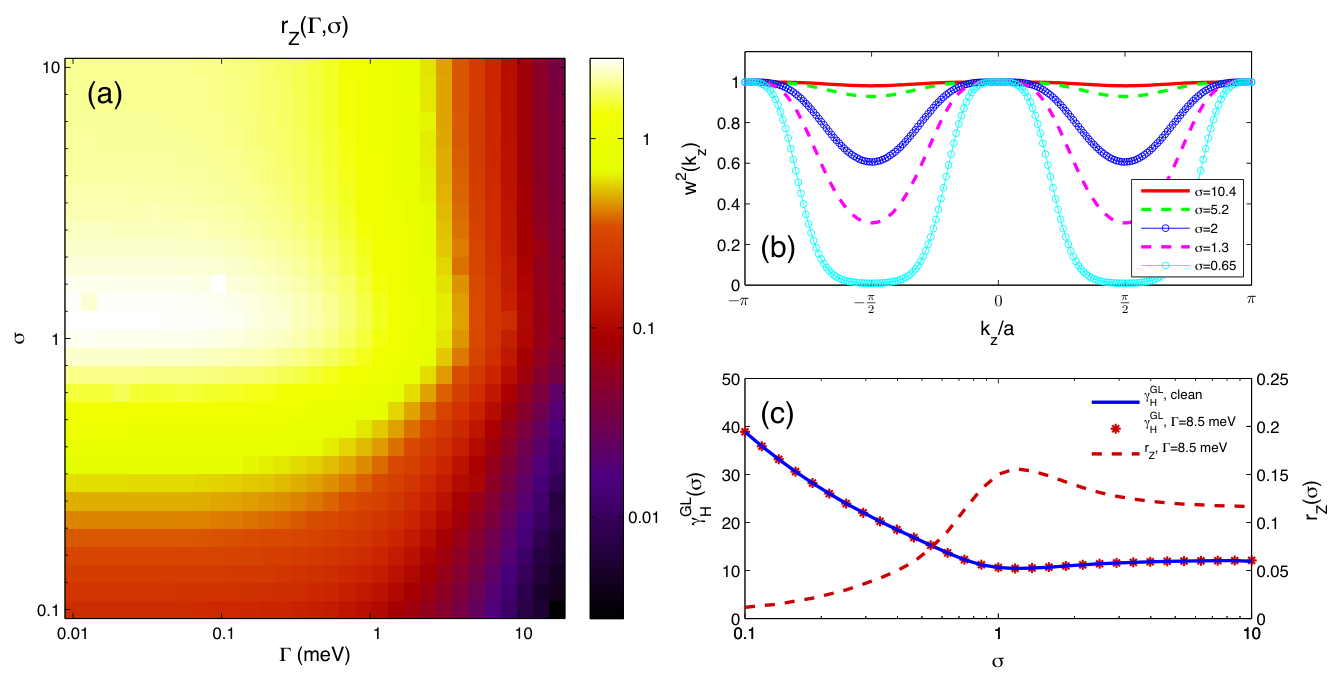
The effective anisotropy parameter $r_{z}$ is maximum at $\Gamma\rightarrow 0$ meV and $\sigma\rightarrow 10$, which represents the clean case and isotropic pairing interaction. Increasing the amount of disorder (i.e. increasing $\Gamma$), as well as squeezing the $w_{\sigma}(k_{z})$ function by reducing its standard deviation $\sigma$, one observes a strong reduction of $r_{z}$. While a significant reduction of $r_{z}$ can be obtained with these two cooperative mechanisms, the experimental estimate of a $r_{z}$ as low as 0.02 would require a marked 2D character of the pairing mechanism, along with a non-negligible residual scattering rate $\Gamma\simeq 10$ meV. While these estimates are not inconsistent with the measured resistivity[32] and with the 2D character of the spin fluctuations above $T_{c}$[22, 31], explaining then paraconductivity experiments[32, 31], the comparison with the experimental findings below $T_{c}$, where the SC properties appear rather isotropic, requires a detailed discussion.

In the previous section we showed that the quasi-2D character of the SCF above $T_{c}$ in LiFeAs can be understood by taking into account the anisotropy of the pairing mechanism along the interlayer direction. A crucial issue is then to compare this result with other estimates of the SC-properties anisotropy done in the literature below $T_{c}$. Here we discuss in details three experiments measuring the upper critical field[33], the critical current[41] and the thermal conductivity[40]. In general, while comparing paraconductivity experiments above $T_{c}$ with other probes below $T_{c}$, two main differences due to the multiband nature of the system must be taken into account. First of all, for what concerns the connection between the pairing mechanism and the SC gap below $T_{c}$, one should consider that when the pairing is mediated by spin fluctuations the Fermi-surface reconstruction due to superconductivity below $T_{c}$ can reduce, within a self-consistent scheme, the anisotropy of the pairing interaction. This implies for example that the gap function below $T_{c}$ can be less anisotropic than what probed by the SCF above $T_{c}$. Second, for what concerns more specifically the behavior of the SCF, for a multiband superconductor the weighted contribution of the various bands to the SCF is not the same for the different experimental probes, in contrast to what happens in a single-band system.

Let us start with the estimate of the anisotropy $\gamma_{H}=H_{c2}^{\perp c}/H_{c2}^{\parallel c}$ between the critical fields perpendicular and parallel to the $c$ axis, respectively[33]. By converting the critical field in the correlation length by using the standard formulas $H_{c2}^{\parallel c}=\Phi_{0}^{2}/2\pi(\xi^{H}_{\parallel})^{2}$ and $H_{c2}^{\perp c}=\Phi_{0}^{2}/2\pi\xi^{H}_{z}\xi_{\parallel}^{H}$ one has:

$$\gamma^{GL}_{H}=\frac{H_{c2}^{\perp c}}{H_{c2}^{\parallel c}}=\left(\frac{\xi^{H}_{\parallel}}{\xi^{H}_{z}}\right)$$

(16)

In a standard single-band superconductor the correlation lengths $\xi_{\parallel}^{H},\xi_{x}^{H}$ which enter the above formula coincide with the ones obtained by the hydrodynamic expansion of the fluctuation propagator (1). Thus, one would estimate

$$\gamma^{GL}_{H}=\left(\frac{4\eta_{\parallel}}{r_{z}d^{2}}\right)^{1/2}$$

(17)

Notice that since $\gamma_{H}^{GL}$ is given by the ratio between the in-plane and out-of-plane stiffness it is rather insensitive to disorder. This is shown in Fig. 1c, where we report the expected single-band-like estimate (17) of $\gamma_{H}^{GL}$ for LiFeAs both in the clean and the dirty case as a function of the pairing anisotropy. We also show in the same plot the anisotropy parameter $r_{z}$ for the dirty case. As one can see, when $r_{z}\simeq 0.02$, that would be consistent with paraconductivity experiments above $T_{c}$, $\gamma^{GL}_{H}$ would be around 20, i.e. much larger than the value $\gamma_{H}\sim 2.5$ obtained experimentally near $T_{c}$. However, in a multiband superconductor one cannot in general identify the $\xi_{\parallel}^{H},\xi_{z}^{H}$ entering Eq. (16) with the ones entering the paraconductivity at zero magnetic field. The reason is the following: the paraconductivity is determined by the hydrodynamic expansion of the SC collective mode which becomes critical at $T_{c}$ at zero magnetic field. Thus, as showed in Ref. [34], one first diagonalizes the multiband problem at zero frequency and momentum to identify the contribution of the various bands to the critical SC mode. Afterwards one expands it at small momenta, to obtain the propagator (1) which enters the leading Aslamazov-Larkin diagrams contributing to the paraconductivity. To solve instead the problem at finite magnetic field one must diagonalize the multiband problem by retaining gradient terms (i.e. the finite-momentum expansion) in the GL propagator for each band. This leads in general to the identification of new multiband effective correlation lengths $\xi_{\parallel}^{H},\xi_{z}^{H}$, where the various bands can contribute with different weights with respect to the zero-field case. A typical example is the two-band case with only interband pairing. The in-plane correlation length entering the paraconductivity can be deduced from Eq. (7), while the upper critical field $H_{c,2}^{\parallel c}$ has been computed in Ref.[35], and reads

$$H_{c,2}^{\parallel}(T)=\frac{24\pi\Phi_{0}T_{c}(T_{c}-T)}{7\zeta(3)\hbar^{2}(v_{e}^{2}+v_{h}^{2})/2}=\frac{\Phi_{0}}{2\pi(\xi_{\parallel}^{H})^{2}}$$

(18)

where $v_{e,h}$ are the velocities of the electron/hole bands, respectively. As a consequence, since $\xi^{2}_{\parallel}\propto\eta_{\parallel}$ and $\eta_{e,h}\propto v_{e,h}^{2}$ from Eq. (3), we obtain:

$$\xi^{2}_{\parallel}\sim\frac{1}{2}(w_{h}^{2}v_{h}^{2}+w_{e}^{2}v_{e}^{2}),\quad(\xi^{H}_{\parallel})^{2}\sim\frac{1}{2}(v_{h}^{2}+v_{e}^{2}).$$

(19)

This means in particular that the two bands contribute equally to $\xi^{H}_{\parallel}$, while this is not the case for $\xi_{\parallel}$. Notice also that the above estimate (18) has been done for two bands with the same mass anisotropy, which is not the case for LiFeAs. Thus, the result for a three-band model as the one used in Sec. II is not known yet, and no conclusions can be reached on the expected values of $\xi_{\parallel}^{H},\xi_{z}^{H}$ in our case. We also note in passing that recently the anisotropy of the correlation length below $T_{c}$ has been inferred also by measurements of the critical current at different magnetic fields[41]. Interestingly, these measurements show an increase of the $\gamma_{H}$ ratio as the magnetic field decreases, with variations near $T_{c}$ by about one order of magnitude between $H=0.5$ T and $H\simeq H_{c2}$. This result could then could reconcile the apparent discrepancy between the paraconductivity, measured at zero field, and the upper-critical fields results.

A second interest comparison can be done with the measurements of the thermal conductivity reported in Ref. [40] Here it has been shown that the thermal transport is quite isotropic in LiFeAs, both for in-plane and out-of-plane heat current. This would rule out any possible gap node or minima for the gap both within the $k_{z}=0$ plane and along the $k_{z}$ direction. However, once more much care should be used to interpret data in a multiband superconductor in terms of a single-band scheme. In particular heat transport in a multiband superconductor is dominated by the band with the smallest gap[44]. Thus, in LiFeAs one would expect a dominant contribution coming from the $\beta$ hole pocket, which is the less interacting one and then less affected by the modulation of the pairing mechanism proposed above.

In summary, we studied a microscopic layered three-band model for the SCF in LiFeAs. By using realistic band parameters, as extracted from the experiments, we showed that the strong 2D character of the SCF found experimentally can be understood as a signature of a strong anisotropy along the inter-plane direction of the pairing interaction, which compensates the low anisotropy of the band dispersion. While within a single-band scenario it would be difficult to reconcile this result with other measurements on the SC anisotropy below $Tc$, the multiband character of pnictides makes such a comparison not straightforward, leaving several questions open for future investigation.

This work has been supported by the Italian MIUR under the project FIRB-HybridNanoDev-RBFR1236VV and the project PRIN-RIDEIRON-2012X3YFZ2, and by the Spanish Ministerio de Economía y Competitividad (MINECO) under the project FIS2011-29680.

References

- [1] Y. Kamihara, T. Watanabe, M. Hirano, and H. Hosono, J. Am. Chem. Soc. 130, 3296 (2008).
- [2] J.Paglione, R.L. Greene Nature 6, 645 (2010)
- [3] G. R. Stewart Rev. Mod. Phys. 83, 1589 (2011)
- [4] A. Chubukov, Annual Review of Condensed Matter Physics Vol. 3: 57-92 (2012)
- [5] P.J. Hirschfeld, M.M Korshunov, and I. Mazin Rep. Prog. Phys. 74, 124508 (2011)
- [6] Y. Xia, D. Qian, L. Wray, D. Hsieh, G.F. Chen, J.L. Luo, N.L. Wang and M.Z. Hasan Phys. Rev. Lett. 103, 037002 (2009)
- [7] H. Kontani and S. Onari, Phys. Rev. Lett. 104, 157001 (2010);
- [8] P.M.R. Brydon, M. Daghofer, C. Timm, and J. van den Brink, Phys. Rev. B83, 060501 (2011).
- [9] T. Saito, S. Onari, Y. Yamakawa, H. Kontani, S.V. Borisenko, V.B. Zabolotnyy arXiv: 1402.2398 (2014)
- [10] M.J. Pitcher, D.R. Parker, P. Adamson, S.J.C. Herkelrath, A.T. Boothroyd, R.M. Ibberson, M. Brunelli and S.J. Clarke Chem. Commun. 2008, 5918 (2008).
- [11] S.V. Borisenko, V.B. Zabolotnyy, D.V. Evtushinsky, T.K. Kim, I.V. Morozov, A.N. Yaresko, A.A. Kordyuk, G. Behr, A. Vasiliev, R. Follath, B. Büchner Phys. Rev. Lett. 105, 067002 (2010).
- [12] K. Umezawa, Y. Lee, H. Miao, K. Nakayama, Z.-H Liu, P. Richard, T. Sato, J.B. He, D.-M. Wang, G.F. Chen, H. Ding, T. Takahashi, and S.-C Wang Phys. Rev. Lett. 108, 037002 (2012).
- [13] T. Hajiri, T. Ito, R. Niwa, M. Matsunami, B. H. Min, Y. S. Kwon, and S. Kimura, Phys. Rev. B 85, 094509 (2012)
- [14] Geunsik Lee, Hyo Seok Ji, Yeongkwan Kim, Changyoung Kim, Kristjan Haule, Gabriel Kotliar, Bumsung Lee, Seunghyun Khim, Kee Hoon Kim, Kwang S. Kim, Ki-Seok Kim, and Ji Hoon Shim , Phys. Rev. Lett. 109, 177001 (2012)
- [15] J. Ferber, K. Foyevtsova, R. Valenti, H.O. Jeschke Phys. Rev. B85, 094505 (2012).
- [16] A.E. Taylor, M.J. Pitcher, R.A. Ewings, T.G. Perring, S.J.Clarke andA.T. Boothroyd, Phys. Rev. B83, 220514 (2011).
- [17] N. Qureshi, P. Steffens, Y. Drees, A.C. Komarek, D. Lamago, Y. Sidis, L. Harnagea, H.-J. Grafe, S. Wurmehl, B. Büchner, M. Braden, Phys. Rev. Lett. 108, 117001 (2012).
- [18] C. Platt, R. Thomale, and W. Hanke, Phys. Rev. B84, 235121 (2011).
- [19] Y. Wang, A. Kreisel, V. B. Zabolotnyy, S. V. Borisenko, B. Büchner, T. A. Maier, P. J. Hirschfeld, and D. J. Scalapino, Phys. Rev. B 88, 174516 (2013)
- [20] G.A. Ummarino, Sara Galasso, D. Daghero, M. Tortello, R.S. Gonnelli, A. Sanna, Physica C: Superconductivity, 492, 15 (2013)
- [21] F. Ahn, I. Eremin, J. Knolle, V. B. Zabolotnyy, S. V. Borisenko, B. Büchner, and A. V. Chubukov Phys. Rev. B 89, 144513 (2014).
- [22] L.Ma, J.Zhang, G.F.Chen, and Weiqiang Yu Phys. Rev. B82, 180501 (2010).
- [23] A.A. Kordyuk, V.B. Zabolotnyy, D.V. Evtushinsky, T.K. Kim, L.V. Morozov, M.L. Kulić, R. Follath, G. Behr, B. Büchner, and S.V. Borisenko, Phys. Rev. B 83, 134513 (2011)
- [24] S.V.Borisenko, V.B.Zabolotnyy, A.A.Kordyuk, D.V.Evtushinsky, T. K. Kim, I. V. Morozov, R. Follath, B. Büchner, Symmetry 4, 251-264 (2012)
- [25] Allan et. al. Science 336, 563 (2012).
- [26] T. Hänke, S. Sykora, R. Schlegel, D. Baumann, L. Harnagea, S. Wurmehl, M. Daghofer, B. Büchner, J. van den Brink, C. Hess, Phys. Rev. Lett. 108, 127001 (2012).
- [27] C. Hess, S. Sykora, T. Hänke, R. Schlegel, D. Baumann, V.B. Zabolotnyy, L. Harnagea, S. Wurmehl, J. van den Brink, B. Büchner Phys. Rev. Lett. 110, 017006 (2013).
- [28] see for example R.I. Rey, A.Ramos-Álvarez, C. Carballeira, J. Mosqueira,F. Vidal, S.Salem-Sugui Jr,A.D. Alvarenga, Rui Zhang, Huiqian Luo, Supercond. Sci. Technol. 27, 075001 (2014) and references therein.
- [29] C. Putzke, A. I. Coldea, I. Guillamón, D. Vignolles, A. McCollam, D. LeBoeuf, M. D. Watson, I. I. Mazin, S. Kasahara, T. Terashima, T. Shib auchi, Y. Matsuda, and A. Carringtón, Phys. Rev. Lett. 108, 047002 (2012).
- [30] B. Zeng, D. Watanabe, Q. R. Zhang, G. Li, T. Besara, T. Siegrist, L. Y. Xing, X. C. Wang, C. Q. Jin, P. Goswami, M. D. Johannes, and L. Balicas, Phys. Rev. B 88, 144518 (2013)
- [31] Yoo Jang Song, Byeongwon Kang, Jong-Soo Rhee, Yong Seung Kwon, Europhys. Lett. 97, 47003 (2012)
- [32] F. Rullier-Albenque, D. Colson, A. Forget, H. Alloul, Phys. Rev. Lett. 109, 187005 (2012).
- [33] B. Lee, S. Khim, JYoo Jang Song, Byeongwon Kang, Jong-Soo Rhee, Yong Seung Kwon Europhys. Lett. 91, 67002 (2010); N. Kurita, K. Kitagawa, K. Matsubayashi, A. Kismarahardja, E.S. Choi, J.S. Brooks, Y. Uwatoko, S. Uji, T. Terashima J. Phys. Soc. Jpn. 80, 013706 (2011); K. Cho, H. Kim, M.A. Tanatar, Y.J. Song, Y.S. Kwon, W.A. Coniglio, C.C. Agosta, A. Gurevich, R. Prozorov Phys. Rev. B83, 060502 (2011); S. Kasahara, K. Hashimoto, H. Ikeda, T. Terashima, Y. Matsuda, and T. Shibauchi, Phys. Rev. B 85, 060503(R) (2012)
- [34] L. Fanfarillo, L. Benfatto, S. Caprara, C. Castellani, and M. Grilli Phys. Rev. B79, 172508 (2009).
- [35] A. Gurevich, Phys. Rev. B82, 184504 (2010).
- [36] N. V. Orlova, A. A. Shanenko, M. V. Milosević, F. M. Peeters, A. V. Vagov, and V. M. Axt, Phys. Rev. B 87, 134510 (2013).
- [37] M. Marciani, L. Fanfarillo, C. Castellani, and L. Benfatto, Phys. Rev. B 88, 214508 (2013)
- [38] L. Fanfarillo, E. Cappelluti, C.Castellani, L. Benfatto, Phys. Rev. Lett. 109, 096402 (2012).
- [39] L. Benfatto and E. Cappelluti, Phys. Rev. B 83, 104516 (2011). L. Benfatto, E. Cappelluti, L. Ortenzi and L. Boeri, Phys. Rev. B 83, 224514 (2011).
- [40] M.A. Tanatar, J.-Ph. Reid, S. Rene de Cotret, N. Doiron-Leyraud, F. Laliberte, E. Hassinger, J. Chang, H. Kim, K. Cho, Yoo Jang Song, Yong Seung Kwon, R. Prozorov, Louis Taillefer Phys. Rev. B84, 054507 (2011).
- [41] M. Konczykowski, C.J. van der Breek, M.A. Tanatar, V. Mosser, Yoo Jang Song, Yong Seung Kwon, R. Prozorov, Phys. Rev. B84, 180514 (2011).
- [42] A. Larkin and A. Varlamov, Theory of fluctuations in superconductors, (Clarendon Press, Oxford, 2005).
- [43] A. E. Koshelev, A. A. Varlamov and V. M. Vinokur, Phys. Rev. B72, 064523 (2005).
- [44] A. A. Golubov and A. E. Koshelev, Phys. Rev. B83, 094521 (2011)
- [45] Y. Zhang, Z.R. Ye, Q.Q. Ge, F. Chen, Juan Jiang, M. Xu, B.P. Xie and D.L. Feng Nat. Phys.8, 371 (2012).
- [46] M.D.Lumsden et al. Phys. Rev. Lett. 102, 107005 (2009).