Occupation numbers in strongly polarized Fermi gases and the Luttinger theorem

Let us start by calculating the in-medium T matrix shown in Fig. 1 within the zero-temperature formalism. As interaction, we consider a contact interaction with coupling constant $g<0$. Then the T matrix can be written as

with $J(\omega,\bm{\mathrm{k}})=J_{\text{hh}}(\omega,\bm{\mathrm{k}})+J_{\text{pp}}(\omega,\bm{\mathrm{k}})$ and

The subscripts hh and pp denote the contributions of hole-hole and particle-particle propagation, respectively. The cutoff $\Lambda$ has been introduced because the momentum integral in $J_{\text{pp}}$ diverges. To be precise, the integration region is defined by $|\bm{\mathrm{p}}-\bm{\mathrm{k}}/2|<\Lambda$, and the upper integration limit in Eqs. (6) and (7) should only be interpreted as a short-hand notation. The usual procedure to deal with the divergence consists in making the coupling constant $g$ dependent on $\Lambda$ and then taking the limit $\Lambda\to\infty$, keeping the scattering length $a$ constant (which implies $g\to 0$) [10]. The result of this renormalization procedure can be written as follows:

where $\tilde{g}=4\pi a/m$, $\tilde{J}=\tilde{J}_{\text{hh}}+\tilde{J}_{\text{pp}}$, $\tilde{J}_{\text{hh}}=\lim_{\Lambda\to\infty}J_{\text{hh}}$, and

The integrals $\tilde{J}_{\text{hh}}$ and $\tilde{J}_{\text{pp}}$ can be evaluated analytically.

Note that within the RPA scheme we should in principle have started from the HF Green’s function instead of the non-interacting one [11]. Consequently, the s.p. energies $\epsilon_{\bm{\mathrm{p}}}$ in Eqs. (6) – (9) should be replaced by HF energies $\epsilon_{\bm{\mathrm{p}}}^{\sigma}=p^{2}/(2m)+gn_{\bar{\sigma}}$, where $\bar{\sigma}$ denotes the spin opposite to $\sigma$. However, as mentioned before, since $g\to 0$ in the limit $\Lambda\to\infty$, we shall not bother with this unnecessary complication.

It is useful to analyze in more detail the properties of $\tilde{J}$ and $\tilde{\Gamma}$. We define the variable $q$ corresponding to the on-shell momentum of each atom in the center of mass (c.m.) frame of the pair, via $\omega=q^{2}/m+k^{2}/(4m)$. In Fig. 3,

we show schematically the regions where the imaginary part of $\tilde{\Gamma}$ is non-zero. The circle corresponds to $\omega=\Omega_{F}=\epsilon^{\uparrow}_{F}+\epsilon^{\downarrow}_{F}$, where $\epsilon_{F}^{\sigma}=k_{F}^{\sigma 2}/(2m)$. This circle separates the regions (1) to (3) (hatched in blue), where the imaginary part comes from $\tilde{J}_{\text{hh}}$, from the regions (4) to (8) (hatched in red), where the imaginary part comes from $\tilde{J}_{\text{pp}}$. On the dashed lines separating the different regions, $\tilde{J}$ has cusps. We see that for $k<k_{F}^{\uparrow}-k_{F}^{\downarrow}$ the hh and pp continua are separated by a region around $\omega=\Omega_{F}$ where the imaginary part vanishes. This is also visible in Fig. 4, where we display the real and imaginary parts of $-\tilde{J}$ for the case $k_{F}^{\downarrow}=k_{F}^{\uparrow}/2$ and $k=0$.

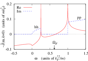
The sharp edges of the hh and pp continua lead to logarithmic singularities in the real part of $\tilde{J}$. Similarly to the original Cooper problem [18], a small attractive interaction ($a<0$) leads therefore to the existence of two poles in $\tilde{\Gamma}$ (at the energies where $-\tilde{J}$ crosses $-1/\tilde{g}$): one slightly below the edge of the pp continuum, corresponding to a bound pair of two particles, and the other slightly above the edge of the hh continuum, corresponding to a bound pair of two holes. These states are shown schematically as the red and blue lines in Fig. 3. With increasing total momentum $k$, the sharp edges are washed out [regions (2) and (7) in Fig. 3] and the poles disappear.

As the interaction strength increases, the upper (pp) pole is shifted to lower and lower energy until it reaches $\omega=\Omega_{F}$. As in the NSR case, this indicates the onset of a pairing instability. If one further increases the interaction strength, the pp pole first enters into the energy range $\omega<\Omega_{F}$ of hh excitations, and then, once $1/\tilde{g}$ drops below the minimum of $-\tilde{J}$, the pole leaves the real $\omega$ axis and becomes complex.

As noticed in in the NSR framework, it is in the imbalanced case not sufficient to consider only $\bm{\mathrm{k}}=0$ in the Thouless criterion (1), but the critical temperature is the highest temperature where the T matrix has a pole at $\omega=\Omega_{F}$ for any value of $\bm{\mathrm{k}}$, related to a transition towards a FFLO-like phase with oscillating order parameter. In the present case we are not interested in the critical temperature (since we are at $T=0$), but in the critical polarization. If we start with a fully polarized system ($P=1$) and decrease the polarization, the critical polarization $P_{c}$ is reached when the T matrix has for the first time a pole at $\omega=\Omega_{F}$ for any value of $\bm{\mathrm{k}}$. Actually it is enough to check that

is fulfilled for all $\bm{\mathrm{k}}$.

Experiments in the unitary limit [5], however, show that the transition from the unpaired to the paired phase at low temperature is not of second, but of first order, leading to phase separation between unpaired and paired phases. Our theory does not allow us to check whether a first-order transition appears already at higher polarization than our $P_{c}$, since this requires a calculation of the energy of the system in the paired phase.

Let us start by writing down the expression for the self-energy diagram shown in Fig. 2(b),

For formal derivations, it will be sometimes convenient to keep the cutoff finite (here, the integration region is defined by $|\bm{\mathrm{p}}-\bm{\mathrm{p}}^{\prime}|/2<\Lambda$), but in all practical calculations we will use the renormalization procedure, i.e., replace $\Gamma$ by $\tilde{\Gamma}$ and let the cutoff $\Lambda$ go to infinity.

To evaluate Eq. (11), it is helpful to split $\Gamma$ into the bare interaction $g$ (which vanishes in the limit $\Lambda\to\infty$) and forward and backward going parts,

Note that in $\Gamma$ the pp and hh channels are summed up together, so that $\Gamma_{\text{pp}}$ contains also contributions from hh propagation and vice versa, as illustrated in Fig. 5.

The separation into forward and backward going parts can be achieved with the help of dispersion relations:

The imaginary parts in the numerators are meant to include also the contribution of possible poles of $\Gamma$ at $\omega=\Omega_{i}$, i.e.,

where the strengths of the poles are given by $S_{i}=1/(dJ/d\omega)_{\Omega_{i}}\sgn(\Omega_{F}-\Omega_{i})$. The self-energy can now also be written as a sum of the energy-independent HF term and forward and backward going parts,

with

In the RPA scheme, the HF term $gn_{\bar{\sigma}}$ must be removed from $\Sigma$ since it is already contained in the HF s.p. energies $\epsilon_{\bm{\mathrm{p}}}^{\sigma}$, but in the limit $\Lambda\to\infty$ it vanishes anyway.

The aim of this section is the calculation of the occupation numbers $n^{\sigma}_{\bm{\mathrm{p}}}$. In terms of the zero-temperature Green’s function, they can be obtained from [9]

If one keeps, as in Eq. (3), only the first-order term of the Dyson equation, one readily obtains

With the help of the residue theorem, this can be written as

One sees that in the case $p>k_{F}^{\sigma}$ only backward going ladders contribute to the occupation numbers (however, remember the remark after Eq. (12)). Likewise, in the case $p<k_{F}^{\sigma}$ only forward going ladders contribute. For the numerical evaluation it is convenient to transform the expressions for the occupation numbers with the help of Eqs. (13) – (18). For $p>k_{F}^{\sigma}$, one gets

Note that the denominator in Eq. (22) cannot become zero because of the upper limit of the $\omega$ integral, the theta function, and the condition $p>k_{F}^{\sigma}$. Analogously, one obtains for $p<k_{F}^{\sigma}$

In this integral, the cutoff can be omitted since the relative momentum of the two particles is anyway limited to $|\bm{\mathrm{k}}/2-\bm{\mathrm{p}}|\leq(k_{F}^{\uparrow}+k_{F}^{\downarrow})/2$ because of the condition $p<k_{F}^{\sigma}$ and the theta function.

In practice, as mentioned before, we replace $\Gamma$ by $\tilde{\Gamma}$ and let the cutoff $\Lambda$ go to infinity. The angular integrals in Eqs. (22) and (23) can be evaluated analytically. The integrals over $\omega$ are split into pole and continuum contributions. The contributions of the delta functions in $\Imag\Gamma$, see Eq. (15), are of course included analytically, while the continuum contributions are computed numerically. The remaining integrals over $k$ are done numerically, too.

As an example, we show in Fig. 6

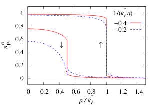
the occupation numbers for $k_{F}^{\downarrow}=k_{F}^{\uparrow}/2$ for two different interaction strengths. We see that the correlations reduce $n^{\sigma}_{\bm{\mathrm{p}}}$ below $k_{F}^{\sigma}$ and generate non-vanishing $n^{\sigma}_{\bm{\mathrm{p}}}$ above $k_{F}^{\sigma}$. This is effect is much stronger for the minority ($\downarrow$) particles than for the majority ($\uparrow$) particles. For $1/(k_{F}^{\uparrow}a)=-0.4$, the occupation numbers look reasonable, but in the more strongly interacting case $1/(k_{F}^{\uparrow}a)=-0.2$ the jump in the $\downarrow$ occupation numbers has the wrong sign. If we increase the interaction further, the $\downarrow$ occupation numbers even become negative below the Fermi surface. This pathological behavior is a consequence of Eq. (3), where the correlations are treated perturbatively by truncating the Dyson equation at first order.

Actually, from Eq. (21) one sees that the jump of $n^{\sigma}_{\bm{\mathrm{p}}}$ is given by

This has to be compared with the exact result

where $Z^{\sigma}_{\bm{\mathrm{p}}}=1/[1-d\Sigma^{\sigma}(\omega,\bm{\mathrm{p}})/d\omega|_{\omega=\epsilon^{\sigma*}_{\bm{\mathrm{p}}}}]$ is the quasiparticle residue of the s.p. Green’s function, with the quasiparticle energy $\epsilon^{\sigma*}_{\bm{\mathrm{p}}}=\epsilon^{\sigma}_{\bm{\mathrm{p}}}+\Sigma^{\sigma}(\epsilon^{\sigma*}_{\bm{\mathrm{p}}},\bm{\mathrm{p}})$ [19]. Equations (24) and (25) agree to leading order in $\Sigma^{\sigma}$ and the change of sign in Eq. (24) for $d\Sigma^{\sigma}/d\omega<-1$ is just a consequence of the breakdown of the expansion $1/(1-d\Sigma^{\sigma}/d\omega)\approx 1+d\Sigma^{\sigma}/d\omega+\dots$.

The Luttinger theorem [12] states that the correlated occupation numbers $n^{\sigma}_{\bm{\mathrm{p}}}$ have their discontinuity still at $k_{F}^{\sigma}=(6\pi^{2}n_{\sigma})^{1/3}$. In other words, if we define

the occupation numbers have to satisfy $\delta n_{\text{h}}^{\sigma}+\delta n_{\text{p}}^{\sigma}=0$.

Using the equations of the preceding subsections and the analytic properties of the different functions in the complex plane, one can show after some transformations that

In the derivation of Eq. (29), we made use of the cutoff regularization, which ensures that $J_{\text{pp}}$ falls off like $1/\omega$ for $\omega\to\infty$. Interestingly, we see that $\delta n_{\text{h}}^{\sigma}$ and $\delta n_{\text{p}}^{\sigma}$ are independent of $\sigma$.

In order to show that the Luttinger theorem is satisfied, we add Eqs. (28) and (29):

Again we have used the cutoff regularization which ensures that $J\to 0$ for $\omega\to\infty$.

The proof can also be carried out with the renormalized functions $\tilde{J}$ and $\tilde{\Gamma}$, but it is more cumbersome in that case. If we integrate numerically our occupation numbers, which are obtained with the renormalized functions, the Luttinger theorem is satisfied to a precision of $\sim 10^{-4}$.

In nuclear physics, the fact that pp-RPA does not modify the sum of particle- and hole occupation numbers in finite nuclei (having discrete particle- and hole levels) has been known for many years, see . Recently, the pp-RPA formalism has been also applied to the case of Bose-Fermi mixtures, and there it was also found that it respects the Luttinger theorem for the Fermion occupation numbers [21].

While in the standard NSR approach the corrections to the densities $n_{\sigma}$ are calculated for fixed chemical potentials $\mu_{\sigma}$, we have just seen that in the zero-temperature formalism there are no corrections to the densities due to correlations. However, there are corrections to the chemical potentials, so that in the end the relationships between $\mu_{\sigma}$ and $n_{\sigma}$ are changed in the zero-temperature formalism, too. If one did a strictly perturbative expansion, i.e., without resummation of ladder diagrams, the difference between the relationships $n_{\sigma}(\mu_{\uparrow},\mu_{\downarrow})$ or, vice versa, $\mu_{\sigma}(n_{\uparrow},n_{\downarrow})$ obtained in the two formalisms should be of higher order than the expansion [19].

Here we will calculate the chemical potentials from the energy density $\mathcal{E}$:

The correlation energy density, $\delta\mathcal{E}=\mathcal{E}-\mathcal{E}_{0}$, where $\mathcal{E}_{0}=(k_{F}^{\uparrow 5}+k_{F}^{\downarrow 5})/(20\pi^{2}m)+gn_{\uparrow}n_{\downarrow}$ is the HF energy density of the uncorrelated system, can be derived from the following general formula [9]

In Eq. (32), $G^{\sigma}_{\lambda}$ denotes the Green’s function calculated with coupling constant $\lambda g$ instead of $g$. More precisely, since RPA theory is built on top of the HF ground state (this is why $\mathcal{E}_{0}$ is not the non-interacting but the HF energy density), the coupling constant entering the HF field must not be multiplied by $\lambda$. Anyway, this detail is not important since the HF field vanishes in the limit $\Lambda\to\infty$.

By inserting Eqs. (3) and (16) (without the HF term $gn_{\bar{\sigma}}$) into Eq. (32), one readily obtains

Using the expressions given in Secs. II.1 and II.2 and exploiting the analytical properties of the functions in the complex plane, one can show that this expression is equal to

Let us now look at the integral over $\lambda$:

Some care has to be taken in the presence of poles in $\Gamma$, since in this case the argument of the logarithm can become negative. In Fig. 4, this corresponds to the region between the hh continuum and the blue line, and between the red line and the pp continuum. In these regions, we have $\Imag\log(1-gJ)=-\pi$. Now Eq. (34) becomes

Although we have assumed in our derivation that $J$ is regularized with a cutoff $\Lambda$, we can now take the limit $\Lambda\to\infty$. In this limit, the contribution of the last term of Eq. (36) vanishes, and we are left with the following compact formula for the correlation energy:

In our calculation of the energy density, the integrals over $k$ and $\omega$ are done numerically (except for the $\omega$ integral of the pole contribution). We have not attempted to derive formulas for the chemical potentials and we compute them by numerically differentiating the energy density.

In Fig. 7,

we show the chemical potentials $\mu_{\uparrow}$ and $\mu_{\downarrow}$ as functions of the polarization $P$ for fixed $n_{\uparrow}$ for different interaction strengths. For each interaction strength, the polarization is varied over the range in which the condition (10) is fulfilled, i.e., $P>P_{c}$. As one would expect, the chemical potential of the minority species, $\mu_{\downarrow}$, is much more strongly lowered by interactions than that of the majority species, $\mu_{\uparrow}$. Actually, already within the “Hartree approximation” ($\mu_{\sigma}=\epsilon_{F}^{\sigma}+\tilde{g}n_{\bar{\sigma}}$) it is like that¹¹ 1 As discussed before, the true HF shift $gn_{\bar{\sigma}}$ vanishes for the regularized contact interaction in the limit $\Lambda\to\infty$. However, in the weak-coupling limit, $\tilde{\Gamma}$ can be approximated by $\tilde{g}$ and this leads to a constant shift $\tilde{g}n_{\sigma}$ which is usually referred to as Hartree shift (there is no exchange term because the interaction acts only between particles of opposite spin).. At the two strongest interactions $1/(k_{F}^{\uparrow}a)=-0.2$ and $-0.1$, one observes that $\mu_{\downarrow}$ increases with decreasing $n_{\downarrow}$ at polarizations $P<0.73$ and $P<0.85$, respectively.

One could be tempted to say that $\partial\mu_{\downarrow}/\partial n_{\downarrow}<0$ indicates an instability towards phase separation into a more and a less polarized phase (first-order phase transition). This would be nice, because experimentally it is found that the system separates into a polarized and an unpolarized phase below some critical polarization [5]. However, the agreement would be purely qualitative since the critical polarization observed in the experiment is much lower than ours (e.g., in the unitary limit, it is about $0.4$ [5]). Furthermore one should remember that at the polarizations where we find $\partial\mu_{\downarrow}/\partial n_{\downarrow}<0$, the truncation of the Dyson equation to first order in $\Sigma$ gives the wrong sign of the jump in the occupation numbers $n_{\bm{\mathrm{p}}}^{\downarrow}$, cf. Fig. 6. If one discards those cases where the jump of $n_{\bm{\mathrm{p}}}^{\downarrow}$ has the wrong sign, one should only consider polarizations $P>0.81$ for $1/(k_{F}^{\uparrow}a)=-0.2$ and $P>0.94$ for $1/(k_{F}^{\uparrow}a)=-0.1$, respectively.

Finally, let us discuss the limit $P\to 1$ (i.e., $n_{\downarrow}\to 0$), corresponding to the polaron. In Fig. 8,

we display our results (pp-RPA) for the polaron energy, which is equal to $\mu_{\downarrow}$ in the limit of $n_{\downarrow}\to 0$, as a function of the interaction strength. These results can be compared with the Hartree approximation $\mu_{\downarrow}=\tilde{g}n_{\uparrow}$ and the results of a calculation by Combescot et al. [22], which are in very good agreement with quantum Monte-Carlo (QMC) results [23, 24]. The calculation of is actually also based on the T matrix, but the polaron energy is defined in a completely different way as the pole of $G^{\downarrow}$ in which the self-energy is summed to all orders. We see that our results represent a considerable improvement over the Hartree approximation and stay very close to the results of up to $1/(k_{F}^{\uparrow}a)\sim-1$.

References

- [1] D.M. Eagles, Phys. Rev. 186, 456 (1969).
- [2] A.J. Leggett, J. Phys. (Paris) 41, C7-19 (1980).
- [3] P. Nozières and S. Schmitt-Rink, J. Low Temp. Phys. 59, 195 (1985).
- [4] M. Greiner, C.A. Regal, and D.S. Jin, Nature 426, 537 (2003).
- [5] Y. Shin, C.H. Schunck, A. Schirotzek, and W. Ketterle, Nature 451, 689 (2008).
- [6] P. Fulde and R.A. Ferrell, Phys. Rev. 135, A550 (1964).
- [7] A.I. Larkin and Yu.N. Ovchinnikov, Sov. Phys. JETP 20, 762 (1965).
- [8] M. Punk, P.T. Dumitrescu, W. Zwerger, Phys. Rev. A 80, 053605 (2009).
- [9] A.L. Fetter and J.D. Walecka, Quantum Theory of Many-Particle Systems (McGraw-Hill, New York, 1971).
- [10] A. Perali, P. Pieri, G.C. Strinati, and C. Castellani, Phys. Rev. B 66, 024510
- [11] P. Ring and P. Schuck, The Nuclear Many-Body Problem (Springer-Verlag, Berlin, 1980)
- [12] J.M. Luttinger, Phys. Rev. 119, 1153 (1960).
- [13] X.-J. Liu, H. Hu, Europhys. Lett. 75, 364 (2006).
- [14] M.M. Parish, F.M. Marchetti, A. Lamacraft, and B.D. Simons, Nature Phys. 3, 124 (2007).
- [15] T. Kashimura, R. Watanabe, and Y. Ohashi, J. Low Temp. Phys. 171, 355 (2013).
- [16] P.-A. Pantel, D. Davesne, and M. Urban, in preparation.
- [17] F. Chevy and C. Mora, Rep. Prog Phys. 73 112401 (2010).
- [18] L.N. Cooper, Phys. Rev. 104, 1189 (1956).
- [19] W.H. Dickhoff and D. Van Neck, Many-Body Theory Exposed! (World Scientific, New Jersey, 2008).
- [20] A. Bouyssy and N. Vinh Mau, Nucl. Phys. A 229, 1 (1974).
- [21] T. Sogo, P. Schuck, and M. Urban, Phys. Rev. A 88, 023613 (2013).
- [22] R. Combescot, A. Recati, C. Lobo, and F. Chevy, Phys. Rev. Lett. 98, 180402 (2007).
- [23] C. Lobo, A. Recati, S. Giorgini, and S. Stringari, Phys. Rev. Lett. 97, 200403 (2006).
- [24] S. Pilati and S. Giorgini, Phys. Rev. Lett. 100, 030401 (2008).
- [25] L.P. Gor’kov and T.K. Melik-Barkhudarov, J. Exp. Theor. Phys. (USSR) 40, 1452 (1961) [translation: Sov. Phys. JETP 13, 1018 (1961)].
- [26] F. Catara, G. Piccitto, M. Sambataro, N. Van Giai, Phys. Rev. B 54, 17536 (1996).
- [27] D.S. Delion, P. Schuck, and J. Dukelsky, Phys. Rev. C 72, 064305 (2005).
- [28] J.G. Hirsch, A. Mariano, J. Dukelsky, and P. Schuck, Ann. Phys. (N.Y.) 296, 187 (2002).
- [29] A. Storozhenko, P. Schuck, J. Dukelsky, G. Röpke, and A. Vdovin, Ann. Phys. (N.Y.) 307, 308 (2003).