跳到论文正文
W Papers独立论文阅读器 arXiv:1407.1991 论文正文 计算阅读时间 · 0%
引用这篇论文根据当前论文元数据生成,正式投稿前建议核对。


License: arXiv.org perpetual non-exclusive license
arXiv:1407.1991v1 [stat.ME] 08 Jul 2014

Rate of uniform consistency for a class of mode regression on functional stationary ergodic data. Application to electricity consumption

Mohamed Chaouch Affiliation:  Department of Statistics, UAE University, United Arab Emirates    Naâmane Laïb & Djamal Louani Affiliation:  L.S.T.A., Université de Paris 6, France.

Abstract - The aim of this paper is to study the asymptotic properties of a class of kernel conditional mode estimates whenever functional stationary ergodic data are considered. To be more precise on the matter, in the ergodic data setting, we consider a random element (X,Z)(X,Z) taking values in some semi-metric abstract space E×FE\times F. For a real function φ\varphi defined on the space FF and x∈Ex\in E, we consider the conditional mode of the real random variable φ⁡(Z)\varphi(Z) given the event `​`​X=x​"``X=x". While estimating the conditional mode function, say θφ​(x)\theta_{\varphi}(x), using the well-known kernel estimator, we establish the strong consistency with rate of this estimate uniformly over Vapnik-Chervonenkis classes of functions φ\varphi. Notice that the ergodic setting offers a more general framework than the usual mixing structure. Two applications to energy data are provided to illustrate some examples of the proposed approach in time series forecasting framework. The first one consists in forecasting the daily peak of electricity demand in France (measured in Giga-Watt). Whereas the second one deals with the short-term forecasting of the electrical energy (measured in Giga-Watt per Hour) that may be consumed over some time intervals that cover the peak demand.

Key words: Conditional mode estimation, energy data, entropy, ergodic processes, functional data, martingale difference, peak load, strong consistency, time series forecasting, vc-classes.

Subject Classifications: 60F10, 62G07, 62F05, 62H15.

1. INTRODUCTION

Let (X,Z)(X,Z) be a E×FE\times F-valued random elements, where EE and FF are some semi-metric abstract spaces. Denote by dEd_{E} and dFd_{F} semi-metrics associated to spaces EE and FF respectively. Let 𝒞{\cal C} be a class of real functions defined upon FF. Obviously, for any φ∈𝒞\varphi\in{\mathcal{C}}, φ⁡(Z)\varphi(Z) is a real random variable. Suppose now that we observe a sequence (Xi,Zi)i≥1(X_{i},Z_{i})_{i\geq 1} of copies of (X,Z)(X,Z) that we assume to be stationary and ergodic. For any x∈Ex\in E and any φ∈𝒞\varphi\in{\mathcal{C}}, let gφ(.|x)g_{\varphi}(.|x) be the conditional density of φ⁡(Z)\varphi(Z) given X=xX=x. We assume that gφ(.|x)g_{\varphi}(.|x) is unimodal on some compact Sφ⊂ℝS_{\varphi}\subset\mathbb{R}. The conditional mode is defined, for any fixed x∈Ex\in E, by

Θφ​(x)=arg​supy∈Sφgφ​(y|x).\Theta_{\varphi}(x)=\mbox{arg}\sup_{y\in S_{\varphi}}g_{\varphi}(y|x).

Note that, if there exists ξ>0\xi>0 such that for any φ∈𝒞\varphi\in\mathcal{C}

gφ(.|x)↑on(Θφ(x)−ξ,Θφ(x))andgφ(.|x)↓on(Θφ(x),Θφ(x)+ξ),\displaystyle g_{\varphi}(.|x)\uparrow\ \mbox{on}\ (\Theta_{\varphi}(x)-\xi,\ \Theta_{\varphi}(x))\ \mbox{and}\ g_{\varphi}(.|x)\downarrow\ \mbox{on}\ (\Theta_{\varphi}(x),\ \Theta_{\varphi}(x)+\xi), (1)

and if we choose Sφ=[Θφ​(x)−ξ,Θφ​(x)+ξ]S_{\varphi}=[\Theta_{\varphi}(x)-\xi,\ \Theta_{\varphi}(x)+\xi], then the mode Θφ​(x)\Theta_{\varphi}(x) is uniquely defined for any φ\varphi. The kernel estimator, say Θ^φ,n​(x)\hat{\Theta}_{\varphi,n}(x), of Θφ​(x)\Theta_{\varphi}(x) may be defined as the value maximizing the kernel estimator gφ,n​(y|x)g_{\varphi,n}(y|x) of gφ​(y|x)g_{\varphi}(y|x), that is,

gφ,n​(Θ^φ,n​(x)|x)=supy∈Sφgφ,n​(y|x).\displaystyle g_{\varphi,n}(\hat{\Theta}_{\varphi,n}(x)|x)=\sup_{y\in S_{\varphi}}g_{\varphi,n}(y|x). (2)

Here,

gφ,n​(y|x)=fφ,n​(x,y)ln​(x),g_{\varphi,n}(y|x)=\frac{{f}_{\varphi,n}(x,y)}{l_{n}(x)},

where

fφ,n​(x,y)=1n​h​𝔼​[Δ1​(x)]​∑i=1n[Δi​(x)​H​(y−φ⁡(Zi)h)],ln​(x)=1n​𝔼​[Δ1​(x)]​∑i=1nΔi​(x)f_{\varphi,n}(x,y)\!=\!\!\frac{1}{nh\mathbb{E}[\Delta_{1}(x)]}\!\!\sum_{i=1}^{n}\!\left[\!\Delta_{i}(x)H\!\left(\!\frac{y-\varphi(Z_{i})}{h}\!\right)\!\right]\!,\!\ l_{n}(x)\!=\!\!\frac{1}{n\mathbb{E}[\Delta_{1}(x)]}\!\sum_{i=1}^{n}\!\Delta_{i}(x)

and Δi​(x)=K​(d⁡(x,Xi)h)\displaystyle{\Delta_{i}(x)=K\left(\frac{d(x,X_{i})}{h}\right)}, with KK and HH two real valued kernels and h:=hnh:=h_{n} a sequence of positive real numbers tending to zero as n→∞n\rightarrow\infty.

The aim of this paper is to establish the uniform consistency, with respect to the function parameter φ∈𝒞\varphi\in{\mathcal{C}}, of the conditional mode estimator Θ^φ,n​(x)\hat{\Theta}_{\varphi,n}(x) when data are assumed to be sampled from a stationary and ergodic process. More precisely, under suitable conditions upon the entropy of the class 𝒞{\mathcal{C}} and the rate of convergence of the smoothing parameter hh together with some regularity conditions on the distribution of the random element (X,Z)(X,Z), we obtain results of type

supφ∈𝒞|Θ^φ,n​(x)−Θφ​(x)|=O⁡(αn),a.s.\sup_{\varphi\in{\mathcal{C}}}|\hat{\Theta}_{\varphi,n}(x)-\Theta_{\varphi}(x)|=O(\alpha_{n}),\ \mbox{a.s.}

where αn\alpha_{n} is a quantity to be specified later on. Notice that, besides the infinite dimensional character of the data, the ergodic framework avoid the widely used strong mixing condition and its variants to measure the dependency and the very involved probabilistic calculations that it implies (see, for instance, Masry (2005)). Further motivations to consider ergodic data are discussed in Laïb (2005) and Laïb & Louani (2010) where details defining the ergodic property of processes together with examples of such processes are also given.

Indexing by a function φ\varphi allows to consider simultaneously various situations related to model fitting and time series forecasting. Whenever Z:={Z⁡(t):t∈T}Z:=\{Z(t):t\in T\} denotes a process defined on some real set TT, one may consider the following functionals φ1​(Z)=supt∈TZ⁡(t)\varphi_{1}(Z)=\sup_{t\in T}Z(t) and φ2​(Z)=inft∈TZ⁡(t)\varphi_{2}(Z)=\inf_{t\in T}Z(t) giving extremes of the process ZZ that are of interest in various domains as, for example, the finance, hydraulics and the weather forecasting. For some weight function WW defined on TT and some p>0p>0, one may consider the functional φp,W\varphi_{p,W} defined by φp,W​(Z)=∫TW⁡(t)​Zp​(t)​𝑑t\varphi_{p,W}(Z)=\int_{T}W(t)Z^{p}(t)dt. Further situation is to consider, for some subset AA of TT, the functional Z→φρ​(Z)=inf{t∈A:Z⁡(t)≥ρ}Z\rightarrow\varphi_{\rho}(Z)=\inf\{t\in A:Z(t)\geq\rho\} for some threshold ρ\rho. Such a case is very useful in threshold and barrier crossing problems encountered in various domains as finance, physical chemistry and hydraulics. Moreover, indexing by a class of functions 𝒞\mathcal{C} is a step towards modelling a functional response random variable. Indeed, the quantity Z⁡(φ):={φ⁡(Z):φ∈𝒞}Z(\varphi):=\{\varphi(Z):\varphi\in\mathcal{C}\} may be viewed as a functional random variable offering, in this respect, a device for such investigations.

The modelization of the functional variable is becoming more and more popular since the publication of the monograph of Ramsay and Silverman (1997) on functional data analysis. Note however that the first results dealing with nonparametric models (mainly the regression function) were obtained by Ferraty and Vieu (2000). Since then, an increasing number of papers on this topic has been published. One may refer to the monograph by Ferraty and Vieu (2006) for an overview on the subject and the references therein. Extensions to other regression issues as the time series prediction have been carried out in a number of publications, see for instance Delsol (2009). The general framework of ergodic functional data has been considered by Laïb and Louani (2010,2011) who stated consistencies with rates together with the asymptotic normality of the regression function estimate.

Asymptotic properties of the conditional mode estimator have been investigated in various situations throughout the literature. Ferraty et al. (2006) studied asymptotic properties of kernel-type estimators of some characteristics of the conditional cumulative distribution with particular applications to the conditional mode and conditional quantiles. Ezzahrioui and Ould Saïd (2008 and 2010) established the asymptotic normality of the kernel conditional mode estimator in both i.i.d. and strong mixing cases. Dabo-Niang and Laksaci (2007) provided a convergence rate in LpL^{p} norm sense of the kernel conditional mode estimator whenever functional α\alpha-mixing observations are considered. Demongeot et al. (2010) have established the pointwise and uniform almost complete convergences with rates of the local linear estimator of the conditional density. They used their results to deduce some asymptotic properties of the local linear estimator of the conditional mode. Attaoui et al. (2011) have established the pointwise and uniform almost complete convergence, with rates, of the kernel estimate of the conditional density when the observations are linked with a single-index structure. They applied their results to the prediction problem via the conditional mode estimate. Notice also that, considering a scalar response variable YY with a covariate XX taking values in a semi-metric space, Ferraty et al. (2010) studied, in the i.i.d. case, the nonparametric estimation of some functionals of the conditional distribution including the regression function, the conditional cumulative distribution, the conditional density together with the conditional mode. They established the uniform almost complete convergence, with rates, of kernel estimators of these quantities.

It is well-known that the conditional mode provides an alternative prediction method to the classical approach based on the usual regression function. Since there exist cases where the conditional density is such that the regression function vanishes everywhere, then it makes no sense to use this approach in problems involving prediction. An example in a finite-dimensional space is given in Ould-Saïd (1997) to illustrate this situation. Moreover, a simulation study in infinite-dimensional spaces carried out by Ferraty et al. (2006), shows that the conditional mode approach gives slightly better results than the usual regression approach.

In this paper, two applications to energy data are provided to illustrate some examples of the proposed approach in time series forecasting framework. The first real case consists in forecasting the daily peak of electricity demand in France (measured in Giga-Watt). Let us denote by (Zi​(t))t∈[0,T](Z_{i}(t))_{t\in[0,T]} the curve of electricity demand (called also load curve) measured over un interval [0,T]. If we have hourly (reps. half-hour) measures then T=24T=24 (resp. T=48T=48). The peak demand observed for any day ii is defined as 𝒫i=supt∈[0,T]Zi​(t)\mathcal{P}_{i}=\sup_{t\in[0,T]}Z_{i}(t). In such case φ⁡(⋅)\varphi(\cdot) is fixed to be the supremum function, over [0,T][0,T], of the function Z⁡(t)Z(t). Accurate prediction of daily peak load demand is very important for decision in the energy sector. In fact, short-term load forecasts enable effective load shifting between transmission substations, scheduling of startup times of peak stations, load flow analysis and power system security studies. Figure 1 provides a sample of seven daily load curves (from 07/01/2002 to 13/01/2002). Vertical dotted lines separate days and the star points correspond to the peak demand for each day.

It is well-known that, in addition to peak demand, some other characteristics of the load curve may be of interest from an operational point of view. In fact the prediction of the electrical energy (measured in Giga-Watt per Hour) consumed over an interval of three hours around the peak demand may helps in the determination of consistent and reliable supply schedules during peak period. Therefore, the second application in this paper deals with the short-term forecasting of the electrical energy that may be consumed between 6pm and 9pm in winter and between 12am and 3pm in summer. Those time intervals cover the peak demand which happens around 7pm in winter and 2pm in summer. Formally, if we consider Zi​(t)Z_{i}(t) the load curve of some day ii, then the electrical energy consumed between t1t_{1} and t2t_{2} is defined as ℰi=∫t1t2Zi​(t)​𝑑t\mathcal{E}_{i}=\int_{t_{1}}^{t_{2}}Z_{i}(t)dt. Therefore, φ⁡(⋅)\varphi(\cdot) in that case is the integral function. A sample of four half hour daily load curves that cover winter and summer seasons is plotted in Figure 2. Solid lines are the daily load curves and the grey surfaces correspond to the electrical energy consumed over an interval of three hours around the peak.

Refer to caption
Figure 1: Half hour electricity consumption in France from 07/01/2002 to 13/01/2002 (7 days). The vertical dotted lines separate days and the star points correspond to the peak demand for each day (in Giga-Watt).
Refer to caption
Figure 2: A sample of four half hour daily load curves that cover winter and summer seasons. Solid lines are the daily load curves and the grey surfaces correspond to the electrical energy (in Giga-Watt per Hour) consumed over an interval of three hours around the peak.

2. RESULTS

In order to state our results, we introduce some notations. Let ℱi{\mathcal{F}}_{i} be the σ\sigma-field generated by ((X1,Z1),…,(Xi,Zi))((X_{1},Z_{1}),\ldots,(X_{i},Z_{i})) and 𝒢i{\mathcal{G}}_{i} the one generated by ((X1,Z1),…CLOSE,((X_{1},Z_{1}),\ldots, OPEN(Xi,Zi),Xi+1)(X_{i},Z_{i}),X_{i+1}). Let B⁡(x,u)B(x,u) be a ball centered at x∈Ex\in E with radius uu. Let Di​(x):=d⁡(x,Xi)D_{i}(x):=d(x,X_{i}) so that Di​(x)D_{i}(x) is a nonnegative real-valued random variable. Working on the probability space (Ω,𝒜,ℙ)(\Omega,{\cal A},\mathbb{P}), let Fx​(u)=ℙ⁡(Di​(x)≤u):=ℙ⁡(Xi∈B⁡(x,u))F_{x}(u)=\mathbb{P}(D_{i}(x)\leq u):=\mathbb{P}(X_{i}\in B(x,u)) and Fxℱi−1​(u)=ℙ⁡(Di​(x)≤u|ℱi−1)=ℙ⁡(Xi∈B⁡(x,u)|ℱi−1)F_{x}^{{\cal F}_{i-1}}(u)=\mathbb{P}(D_{i}(x)\leq u\ |{\cal F}_{i-1})=\mathbb{P}(X_{i}\in B(x,u)\;|{\cal F}_{i-1}) be the distribution function and the conditional distribution function, given the σ\sigma-field ℱi−1{\cal F}_{i-1}, of (Di​(x))i≥1(D_{i}(x))_{i\geq 1} respectively. Denote by oa.s.​(u)o_{\mbox{a.s.}}(u) a real random function ll such that l⁡(u)/ul(u)/u converges to zero almost surely as u→0u\rightarrow 0. Similarly, define Oa.s.​(u)O_{\mbox{a.s.}}(u) as a real random function ll such that l⁡(u)/ul(u)/u is almost surely bounded.

Our results are stated under some assumptions we gather hereafter for easy reference.

  1. A1

    For x∈Ex\in E, there exist a sequence of nonnegative random functional (fi,1)i≥1(f_{i,1})_{i\geq 1} almost surely bounded by a sequence of deterministic quantities (bi​(x))i≥1(b_{i}(x))_{i\geq 1} accordingly, a sequence of random functions (ψi,x)i≥1(\psi_{i,x})_{i\geq 1}, a deterministic nonnegative bounded functional f1f_{1} and a nonnegative nondecreasing real function ϕ\phi tending to zero as its argument goes to zero, such that

    • (i)

      Fx​(u)=ϕ⁡(u)​f1​(x)+o⁡(ϕ⁡(u))\displaystyle{F_{x}(u)=\phi(u)f_{1}(x)+o(\phi(u))}, as u→0u\rightarrow 0,

    • (ii)

      For any i∈ℕi\!\in\!\mathbb{N}, Fxℱi−1​(u)=ϕ⁡(u)​fi,1​(x)+ψi,x​(u)\displaystyle{F_{x}^{\mathcal{F}_{i-1}}(u)\!=\!\phi(u)f_{i,1}(x)+\psi_{i,x}}(u) with ψi,x​(u)=oa.s.​(ϕ⁡(u))\psi_{i,x}(u)\!=\!o_{a.s.}(\phi(u)) as u→0u\!\rightarrow\!0, ψi,x​(u)ϕ⁡(u)\displaystyle{\frac{\psi_{i,x}(u)}{\phi(u)}} is almost surely bounded and 1n​∑i=1nψi,x​(u)=oa.s.​(ϕ⁡(u))\displaystyle{\frac{1}{n}\!\sum_{i=1}^{n}\!\psi_{i,x}(u)\!=\!o_{a.s.}(\phi(u))} as n→∞n\rightarrow\infty, u→0u\rightarrow 0.

    • (iii)

      n−1​∑i=1nfi,1​(x)→f1​(x)\displaystyle{n^{-1}\sum_{i=1}^{n}f_{i,1}(x)}\rightarrow f_{1}(x) almost surely as n→∞n\rightarrow\infty.

    • (iv)

      There exists a nondecreasing bounded function τ0\tau_{0} such that, uniformly in u∈[0, 1]u\in[0,\ 1],
      ϕ⁡(h​u)ϕ⁡(h)=τ0​(u)+o⁡(1)\displaystyle{\frac{\phi(hu)}{\phi(h)}\!=\!\tau_{0}(u)\!+\!o(1)}, as h↓0h\downarrow 0 and, for ≤j≤21\!\leq\!j\!\leq 2, ∫01(Kj​(u))′​τ0​(u)​𝑑u<∞\displaystyle{\int_{0}^{1}\!\!(K^{j}(u))^{\prime}\tau_{0}(u)du\!<\!\infty}.

    • (v)

      n−1​∑i=1nbi​(x)→D⁡(x)<∞n^{-1}\sum^{n}_{i=1}b_{i}(x)\rightarrow D(x)<\infty as n→∞n\rightarrow\infty.

  2. A2

    KK is a nonnegative bounded kernel of class 𝒞1\mathcal{C}^{1}\! over its support [0,1][0,1], with K⁡(1)>0K(1)\!>\!0 and the derivative K′K^{\prime}\! is such that K′​(t)<0K^{\prime}\!(t)\!<\!0, for any t∈[0,1]t\in[0,1].

  3. A3
    • (i)

      For any ϵ>0\epsilon>0, there exists η>0\eta>0 such that for any (φ1,φ2)∈𝒞×𝒞(\varphi_{1},\ \varphi_{2})\in\mathcal{C}\times\mathcal{C}, d𝒞​(φ1,φ2)<ηd_{\mathcal{C}}(\varphi_{1},\ \varphi_{2})<\eta implies that |Θφ1​(x)−Θφ2​(x)|<ϵ|\Theta_{\varphi_{1}}(x)-\Theta_{\varphi_{2}}(x)|<\epsilon.

    • (ii)

      Uniformly in φ∈𝒞\varphi\in\mathcal{C}, gφ(.|x)g_{\varphi}(.|x) is uniformly continuous on SφS_{\varphi}.

    • (iii)

      gφ(.|x)g_{\varphi}(.|x) is differentiable up to order 22 and limn→∞supφ∈𝒞|gφ(2)​(Θ^φ,n​(x)|x)|:=Φ⁡(x)≠0\lim_{n\to\infty}\displaystyle{\sup_{\varphi\in\mathcal{C}}|g_{\varphi}^{(2)}(\hat{\Theta}_{\varphi,n}(x)|x)|\!:=\!\Phi(x)\!\neq\!0}.

    • (iv)

      For any x∈Ex\in E, there exist V⁡(x)V(x) a neighborhood of xx, some constants Cx>0C_{x}>0, β>0\beta>0 and ν∈(0, 1]\nu\in(0,\ 1], independent of φ\varphi, such that for any φ∈𝒞\varphi\in\mathcal{C}, we have ∀(y1,y2)∈Sφ×Sφ\forall\ (y_{1},\ y_{2})\in S_{\varphi}\times S_{\varphi}, ∀(x1,x2)∈V⁡(x)×V⁡(x)\forall(x_{1},\ x_{2})\in V(x)\times V(x),

      |gφ(j)(y1|x1)−gφ(j)(y2|x2)|≤Cx(|y1−y2|ν+d(x1,x2)β),j=0,2.|g^{(j)}_{\varphi}(y_{1}|x_{1})-g^{(j)}_{\varphi}(y_{2}|x_{2})|\leq C_{x}(|y_{1}-y_{2}|^{\nu}+d(x_{1},\ x_{2})^{\beta}),\ j=0,2.

  4. A4

    The kernel HH is such that

    1. (i)

      ∫ℝ|t|ν​H​(t)​𝑑t<∞\displaystyle{\int_{\mathbb{R}}|t|^{\nu}H(t)dt<\infty} and ∫ℝt​H​(t)​𝑑t=0\displaystyle{\int_{\mathbb{R}}tH(t)dt=0},

    2. (ii)

      ∀(t1,t2)∈ℝ2,|H⁡(t1−φ1​(z))−H⁡(t2−φ2​(z))|≤CH​(|t1−t2|+d𝒞​(φ1,φ2))\displaystyle{\forall\ (t_{1},t_{2})\!\in\!\mathbb{R}^{2},|H(t_{1}\!-\!\varphi_{1}(z))\!-\!H(t_{2}\!-\!\varphi_{2}(z))|\!\leq\!C_{H}(|t_{1}\!-\!t_{2}|\!+\!d_{\mathcal{C}}(\varphi_{1},\varphi_{2}))}, where CHC_{H} is a positive constant.

  5. A5

    For j=0,1,2j=0,1,2 and any φ∈𝒞\varphi\in{\cal C},

    𝔼⁡[H(j)​(y−φ⁡(Zi)h)∣𝒢i−1]=𝔼⁡[H(j)​(y−φ⁡(Zi)h)∣Xi].\mathbb{E}\left[H^{(j)}\left(\frac{y-\varphi(Z_{i})}{h}\right)\mid\mathcal{G}_{i-1}\right]=\mathbb{E}\left[H^{(j)}\left(\frac{y-\varphi(Z_{i})}{h}\right)\mid\ X_{i}\right].

Comments on the hypotheses. As to discuss the conditions A1, it is worth noticing that the fundamental hypothesis A1(ii) involves the functional nature of the data together with their dependency. As usually in such a framework, small balls techniques are used to handle the probabilities on infinite dimension spaces where the Lebesgue measure does not exist. Several examples of processes fulfilling this condition are given in Laïb & Louani (2011). Note that the hypothesis A1(i) stands as a particular case of A1(ii) while conditioning by the trivial σ\sigma-field. A number of processes satisfying this condition are given through out the literature, see, for instance, Ferraty & Vieu (2006). Conditions A1(iii) and A1(v) are set basically to meet the ergodic Theorem which may be expressed as the classical law of large numbers. Conditions A2 and A4 impose some regularity conditions upon the kernels used in our estimates. When indexing by a class of functions 𝒞\mathcal{C}, it is natural to consider regularity conditions as the continuity of the mode with respect to the index function φ\varphi assumed in A3(i). Defined as an argmax and, furthermore, indexed by the class 𝒞\mathcal{C}, the conditional mode is sensitive to fluctuations. The diffrentiability of the conditional density gφg_{\varphi} with some kind of smoothness of its derivatives is needed to reach the rates of the convergence obtained in our results. All these conditions are summarised in the assumption A3. Hypothesis A5 is of Markov’s nature.

Before establishing the uniform convergence with rate, with respect to the class of functions 𝒞{\cal C}, of the conditional mode estimator, we introduce the following notation. For any ϵ>0\epsilon>0, set

𝒩⁡(ϵ,𝒞,d)\displaystyle{\cal N}(\epsilon,{\cal C},d) =\displaystyle= min{n:there existc1⋯,cnin𝒞such that∀φ∈𝒞\displaystyle\min\{n:\ \mbox{there exist}\ c_{1}\cdots,c_{n}\ \mbox{in}\ {\cal C}\ \mbox{such that}\ \forall\ \varphi\in{\cal C}
 there exists 1≤k≤nsuch thatd(φ,ck)<ϵ}.\displaystyle\hskip 36.98866pt\ \mbox{ there exists}\ 1\leq k\leq n\ \mbox{such that}\ d(\varphi,c_{k})<\epsilon\}.

This number measures how full is the class 𝒞{\cal C}. Obviously, conditions upon the number 𝒩⁡(ϵ,𝒞,d){\cal N}(\epsilon,{\cal C},d) have to be set to state uniform over the class 𝒞{\cal C} results.

The following proposition establishes the uniform asymptotic behavior (with rate) of the conditional density estimator g⁡(y|x)g(y|x) with respect to y and the function φ∈𝒞\varphi\in{\cal C}. This proposition which is of interest by itself may be used, as an intermediate result, to prove our main result given in Theorem 1 below.

Proposition 1

Under conditions A1, A2, A3, A4 and A5 together with hypotheses (3)-(4), we have

supφ∈𝒞supy∈Sφ|gφ,n​(y|x)−gφ​(y|x)|\displaystyle\sup_{\varphi\in\mathcal{C}}\sup_{y\in S_{\varphi}}|g_{\varphi,n}(y|x)-g_{\varphi}(y|x)| =\displaystyle= Oa.s​(hβ+hν)+Oa.s.​(η​h−2)+Oa.s.​(λn)\displaystyle O_{a.s}(h^{\beta}+h^{\nu})+O_{a.s.}\left(\eta h^{-2}\right)+O_{a.s.}\left(\lambda_{n}\right)
+Oa.s​((log⁡nn​ϕ​(h))1/2).\displaystyle\ \ +O_{a.s}\left(\left(\frac{\log n}{n\phi(h)}\right)^{1/2}\right).

Our principal result considers the pointwise in x∈ℰx\in{\cal E} and uniform over the class 𝒞\mathcal{C} convergence of the kernel estimate Θ^φ,n​(x)\hat{\Theta}_{\varphi,n}(x) of the conditional mode Θφ​(x)\Theta_{\varphi}(x).

Theorem 1

Assume that the conditions A1-A5 hold true and that

limn→∞log⁡(n)n​ϕ​(h)=0.\displaystyle\lim_{n\rightarrow\infty}\frac{\log(n)}{n\phi(h)}=0. (3)

Furthermore, for a sequence of positive real numbers λn\lambda_{n} tending to zero, as n→∞n\rightarrow\infty, and η=ηn=O⁡(h2+β)\eta=\eta_{n}=O(h^{2+\beta}), with β>0\beta>0, suppose that

(i)limn→∞log⁡𝒩⁡(η,𝒞,d)η​λn2​n​h​ϕ​(h)=0and(i​i)∑n≥1exp⁡{−λn2​O​(n​h​ϕ​(h))}<∞.(i)\ \ \lim_{n\rightarrow\infty}\frac{\log{\cal N}(\eta,{\cal C},d)}{\eta\lambda_{n}^{2}nh\phi(h)}=0\ \ \mbox{and}\ \ \ (ii)\ \ \sum_{n\geq 1}\exp\{-\lambda_{n}^{2}O(nh\phi(h))\}<\infty. (4)

Then, as n→∞n\rightarrow\infty, we have

supφ∈𝒞|Θ^φ,n​(x)−Θφ​(x)|=Oa.s​(hβ/2+hν/2)+Oa.s​(λn12)+Oa.s​((log⁡nn​ϕ​(h))1/4).\sup_{\varphi\in\mathcal{C}}|\hat{\Theta}_{\varphi,n}(x)-\Theta_{\varphi}(x)|=O_{a.s}(h^{\beta/\!2}+h^{\nu/\!2})+O_{a.s}\left(\lambda_{n}^{\frac{1}{2}}\right)+O_{a.s}\left(\left(\frac{\log n}{n\phi(h)}\right)^{1/4}\right).
Remark 1

Replacing the condition (4)(i) by limn→∞log⁡𝒩⁡(η,𝒞,d)η​λn2​n​h​ϕ​(h)=δ\displaystyle{\lim_{n\rightarrow\infty}\frac{\log{\cal N}(\eta,{\cal C},d)}{\eta\lambda_{n}^{2}nh\phi(h)}=\delta}, for some δ>0\delta>0, with λn=O⁡((log⁡nn​h​ϕ​(h))12)\displaystyle{\lambda_{n}=O\left(\left(\frac{\log n}{nh\phi(h)}\right)^{\frac{1}{2}}\right)}, the condition (4)(ii) is clearly satisfied inducing the uniform consistency, with respect to φ∈𝒞\varphi\in\mathcal{C}, of Θ^φ,n​(x)\hat{\Theta}_{\varphi,n}(x) with the rate

Oa.s.​(hβ/2+hν/2)+Oa.s.​((log⁡nn​ϕ​(h))14)\displaystyle{O_{\mbox{a.s.}}(h^{\beta/\!2}+h^{\nu/\!2})+O_{\mbox{a.s.}}\left(\left(\frac{\log n}{n\phi(h)}\right)^{\frac{1}{4}}\right)}

.

Remark 2

Note, whenever η=O⁡(h2+β)\eta=O(h^{2+\beta}) and λn−1=O⁡((n​h5+2​β​ϕ​(h))12)\lambda_{n}^{-1}=O((nh^{5+2\beta}\phi(h))^{\frac{1}{2}}), that the condition (4)(i) takes the form

limη→0η​log⁡𝒩⁡(η,𝒞,d)=0.\lim_{\eta\rightarrow 0}\eta\log{\cal N}(\eta,{\cal C},d)=0. (5)

The condition (5) is very usual in defining Vapnik-Chervonenkis classes. Examples of classes fulfilling the condition (5) are given throughout the literature, see, for instance, Laïb & Louani (2011) and van der Vart & Wellner (1996).

2.1 Application to time series forecasting

The main application of Theorem 1 is devoted to prediction of time series when considering the conditional mode estimates.

For n∈ℕ⋆n\in\mathbb{N}^{\star}, let Zi​(t)Z_{i}(t) and Xi​(t)X_{i}(t), i=1,…,ni=1,\dots,n, be two functional random variables with t∈[0,T).t\in[0,T). For each curve Xi​(t)X_{i}(t) (the covariate), we have a real response Yφ,i=φ⁡(Zi​(t))Y_{\varphi,i}=\varphi(Z_{i}(t)), a transformation of some functional variable Zi​(t)Z_{i}(t). Given a new curve Xn+1=xnewX_{n+1}=x_{\mbox{new}}, our purpose is to predict the corresponding response yφ,new:=Θφ​(xnew)y_{\varphi,\mbox{new}}:=\Theta_{\varphi}(x_{\mbox{new}}) using as predictor the conditional mode, say y^φ,new:=Θ^φ,n​(xnew)\widehat{y}_{\varphi,\mbox{new}}:=\widehat{\Theta}_{\varphi,n}(x_{\mbox{new}}). The following Corollary based on Theorem 1 gives the asymptotic behavior with rate of the empirical error prediction.

Corollary 1

Assume that conditions of Theorem 1 hold. Then we have

|y^φ,new−yφ,new|=Oa.s​(hβ/2+hν/2)+Oa.s​(λn12)+Oa.s​((log⁡nn​ϕ​(h))1/4).\Big|\widehat{y}_{\varphi,\mbox{new}}-y_{\varphi,\mbox{new}}\Big|=O_{a.s}(h^{\beta/\!2}+h^{\nu/\!2})+O_{a.s}\left(\lambda_{n}^{\frac{1}{2}}\right)+O_{a.s}\left(\left(\frac{\log n}{n\phi(h)}\right)^{1/4}\right).

Proof. The proof of Corollary 1 is a direct consequence of Theorem 1.

3. APPLICATIONS TO REAL DATA

The data-set analyzed in this paper contains half hourly observations of a stochastic process ξ⁡(t)\xi(t), t∈ℝ+t\in\mathbb{R}^{+}. Here ξ⁡(t)\xi(t) represents the electricity demand at time tt in France. This process has been observed at each half hour from 01 January 2002 to 31 December 2005 (which corresponds to a total of 1461 days). Figure 3 shows the evolution of the process ξ⁡(t)\xi(t) over time. One can easily see a high seasonality since the variation of the electricity consumption is due to the climatic conditions in France. In fact, the winter and autumn are rather cold, whereas the climate in summer and spring is relatively warm. This remark is confirmed by Figure 4 which displays the half hourly electricity consumption in France in four selected weeks. We can clearly distinguish the intra-daily periodical pattern, and we can also note the difference in terms of level of consumption from one season to another. The repetitiveness of the daily shape is due to a certain inertia in the demand that reflects the aggregated behavior of consumers.

Refer to caption
Figure 3: Half hour electricity consumption in France from 07/01/2002 to 31/12/2005 generated according to the process ξ⁡(t)\xi(t).
Refer to caption
Figure 4: Half hour electricity demand in four selected weeks (the panel contains one week data from January, April, August and October 2004).

Theoretically the evolution of the energy data was observed according to the process ξ⁡(t)\xi(t). Now in order to construct our functional data Z⁡(t)Z(t) and to get its transformation φ⁡(Z⁡(t))\varphi(Z(t)) we proceed by slicing the original process ξ⁡(t)\xi(t) into segments of similar length. Since our target is a day-ahead short term forecasting we divide the observed original time series (ξ⁡(t)\xi(t)) of half hourly electricity consumption into n=1461n=1461 segments (Z(t)) of length 4848 which correspond to the functional observations. Each segment coincident with a specific daily load curve. Formally, let [0,T][0,T] the time interval on which the process ξ⁡(t)\xi(t) is observed. We divide this interval into subintervals of length 48, say [ℓ×48,(ℓ+1)×48][\ell\times 48,(\ell+1)\times 48], ℓ=0,1,…,n−1\ell=0,1,\dots,n-1, with n=T/48=1461n=T/48=1461. Denoting by Zi​(t)Z_{i}(t) the functional-valued discrete-time stochastic process defined by

Zi(t)=ξ(t+(i−1)×48);i=1,…,n,∀t∈[0,48).\displaystyle Z_{i}(t)=\xi(t+(i-1)\times 48);\quad\quad i=1,\dots,n,\quad\forall t\in[0,48). (6)

Figure 5 shows a, randomly chosen, sample of 20 realizations of the functional random variable (Z⁡(t))t∈[0,48)(Z(t))_{t\in[0,48)} which corresponds to a daily load curves.

Refer to caption
Figure 5: A sample of 20 daily load curves randomly chosen generated according to the process Z⁡(t)Z(t).

Once we have transformed our original time series into functional data type, one can start, as explained in the introduction, dealing with the short term forecasting of the daily peak demand and the electrical energy consumed over an interval using the conditional mode as predictor.

3.2 Short-term daily peak load forecasting

Let us now consider the observed daily peak of the electricity consumption defined, for any day i=1,…,ni=1,\dots,n, as

𝒫i=supt∈[0,48)Zi​(t).\displaystyle\mathcal{P}_{i}=\sup_{t\in[0,48)}Z_{i}(t).

The goal of this subsection is to forecast the peak 𝒫i\mathcal{P}_{i} on the basis of the load curve of the previous day, Zi−1​(t)Z_{i-1}(t). Forecasting peak load demand is one of the most relevant issues in electricity companies. In fact, the electricity market is more and more open to competition and companies take care on the quality of their services in order to increase the number of their customers. On the other hand, because of the electrification of appliances (e.g. electric heating, air conditioning, …) and mobility applications (e.g. electric vehicle, …), the peak demand is increasing which can leads to a serious issues in the electric network. It is important, therefore, to produce very accurate short-term peak demand forecasts for the day-to-day operation, scheduling and load-shedding plans of power utilities. Forecasting peak load toke a lot of interest in the statistical literature. For instance Goia et al. (2010) used a functional linear regression model and Sigauke & Chikobvu (2010) a multivariate adaptive regression splines model. These methods are based on the regression function as a predictor, here we suggest the mode regression as an alternative.

In this paper, we compare two predictors based on different choices of the covariable X⁡(t)X(t). Since the peak electricity demand is highly correlated to the electricity consumption of the previous day and also to the temperature measures, we have then two possibilities to chose the covariable X⁡(t)X(t):

Refer to caption
Figure 6: Results for one year day-ahead forecasting of the daily peak electricity demand using as predictor the mode regression and as functional covariate: (a) the curve of electricity consumption of the previous day (Prev.Day), (b) the predicted half hourly temperature curve of the target day (Pred.Temp.).
Refer to caption Refer to caption
              (a)               (b)
Figure 7: Examples of daily peak load forecast using conditional mode, conditional median and regression function for eight consecutive days

To evaluate the proposed approach, we split the sample of n=1461n=1461 days into:

Remark 3

When the functional covariate is fixed to be the predicted temperature curve, say T^​(t)\widehat{T}(t), the notations for the learning and test sample can be changed as follow: ℒ={(T^i​(t),𝒫i)}i=1,…,1096\mathcal{L}=\{(\widehat{T}_{i}(t),\mathcal{P}_{i})\}_{i=1,\dots,1096} and 𝒯={(T^i​(t),𝒫i)}1,…,365\mathcal{T}=\{(\widehat{T}_{i}(t),\mathcal{P}_{i})\}_{1,\dots,365}.

Table 1: Distribution (by month) of the RAE of the peak load obtained by using as predictor the conditional mode and as covariate the previous day Prev.Day and predicted temperature Pred.Temp.
Prev.Day(%) Pred.Temp.(%)
MAPEm\texttt{MAPE}_{m} Q0.25Q_{0.25} Q0.5Q_{0.5} Q0.75Q_{0.75} MAPEm\texttt{MAPE}_{m} Q0.25Q_{0.25} Q0.5Q_{0.5} Q0.75Q_{0.75}
Jan. 4.2 1.4 3.1 5.2 9.5 5.4 9.4 14.2
Feb. 5.4 1.9 4.0 8.3 6.9 1.3 6.3 10.2
Mar. 6.1 2.0 3.7 8.0 9.0 3.5 6.5 13.3
Apr. 6.7 2.6 4.9 9.4 11.9 6.0 11.4 18.2
May 4.7 0.5 1.5 9.5 9.9 3.2 8.0 14.1
Jun. 2.4 0.7 1.2 2.2 9.3 3.5 7.7 15.5
Jul. 3.1 0.5 1.5 3.2 8.3 2.2 7.4 11.2
Aug. 3.0 0.6 1.3 3.6 11.1 4.6 8.0 14.2
Sep. 2.5 0.3 0.8 1.7 10.9 4.0 9.5 18.7
Oct. 4.0 0.9 2.3 4.4 11.0 4.5 9.9 17.5
Nov. 5.4 2.0 3.9 7.1 8.9 3.7 6.8 14.1
Dec. 5.9 2.2 5.5 8.2 7.1 3.2 5.8 9.3

The learning sample is used to build the proposed estimator given by (2) and to find the “optimal” smoothing parameter. To estimate the conditional mode some tuning parameters should be fixed. We suppose here that the kernel (resp. the smoothing parameter) for both the covariate and the response variable is the same and considered to be the quadratic kernel defined as K⁡(u)=H⁡(u)=1.5​(1−u2)​1​l[0,1]K(u)=H(u)=1.5(1-u^{2})1\kern-1.99997pt{\rm l}_{[0,1]} (resp. h:=hK=hHh:=h_{K}=h_{H}). The optimal bandwidth hh is obtained by the cross-validation method on the kk-nearest neighbors (see Ferraty and Vieu (2006), p. 102 for more details). Finally, the semi-metric d⁡(⋅,⋅)d(\cdot,\cdot) is fixed to be the L2L_{2} distance between the second derivative of the curves.

The test sample will be used to compare our forecasts to the observed daily peak electricity demand for the year 2005. Figure 6(a) (resp. (b)) displays the observed and the predicted values of the daily peak electricity demand using as covariable the load curve of the previous day (reps. the predicted temperature curve). Since cross-points, (𝒫^i,𝒫i)i=1,…,365(\widehat{\mathcal{P}}_{i},\mathcal{P}_{i})_{i=1,\dots,365}, represented in Figure 6(a) are more concentrated on the diagonal line than those in Figure 6(b), one can deduce that the first approach provides better results than the second one. Moreover, Table 1 provides a numerical summary of the RAE obtained by using as covarite the predicted temperature curve or the last observed daily load curve. One can observe that monthly errors obtained by the second approach are usually less than those given by the first one. Therefore, one can conclude that the peak electricity demand might be better modelized by the previous daily load curve rather than by the predicted temperature curve.

Following the previous analysis, the last observed daily load curve will be be considered, in the rest of this section, as the suitable covariate to forecast the peak demand. Our goal, now, consists in comparing the conditional mode predictor to the conditional median and the regression function (conditional mean) (see Ferraty and Vieu (2006) for more details about the properties of those last two predictors).

For a deeper analysis and evaluation of the accuracy of the proposed approach we use as validation criterias: the Relative Absolute Errors (RAE) and the monthly Mean Absolute Prediction Error (MAPEm\texttt{MAPE}_{m}), defined respectively, for any day i=1,…,365i=1,\dots,365, in the test sample, as

RAEi=|𝒫i−𝒫^i|𝒫iandMAPEm=1Nm​∑i=1Nm|𝒫i−𝒫^i|𝒫i\texttt{RAE}_{i}=\frac{|\mathcal{P}_{i}-\widehat{\mathcal{P}}_{i}|}{\mathcal{P}_{i}}\quad\quad\mbox{and}\quad\quad\texttt{MAPE}_{m}=\frac{1}{N_{m}}\sum_{i=1}^{N_{m}}\frac{|\mathcal{P}_{i}-\widehat{\mathcal{P}}_{i}|}{\mathcal{P}_{i}}

where NmN_{m} is a number of days for a given month m∈{1,…,12}m\in\{1,\dots,12\} and 𝒫^i\widehat{\mathcal{P}}_{i} is the predicted value of the daily peak obtained by the conditional mode, conditional median or regression function.

Figure 8 shows examples of peak load forecasts for eight consecutive days. One can see that conditional mode provides more accurate predictions than the two other methods. In Figure 7 the 365 forecasted daily peak load are plotted against the observed ones. Clearly, one can observe that conditional mode performs well the forecasts while conditional median and regression function under-predict peak in the cold season and over-predict it in hot season.

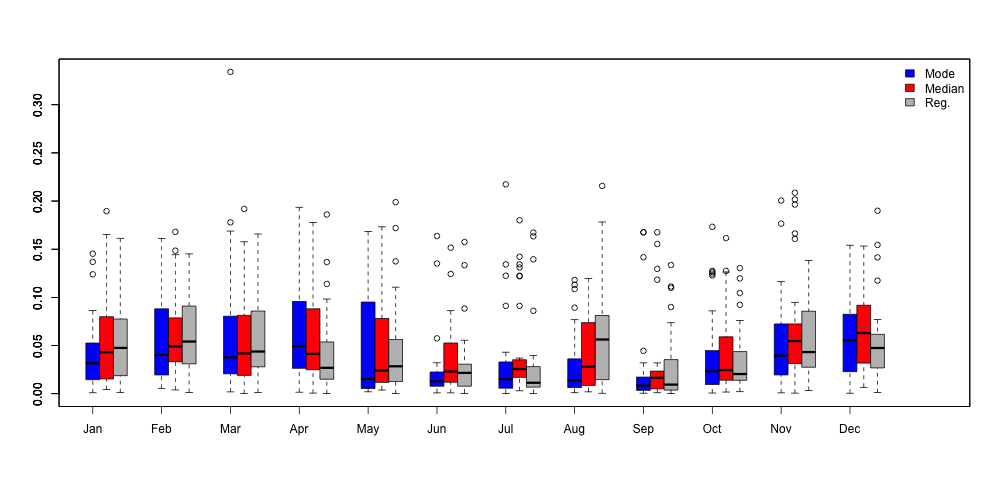
Figure 9 provides the distribution of the daily RAE for each month in 2005, obtained by using the three prediction methods. One can observe that the conditional mode-based approach is much more efficient in winter, as well as, in summer, than the other methods. Accurate forecasts in winter are of particular interest since the last is the period of the year whenever electricity demand might exceed the supply capacity and therefore efficient energy management in the electrical grid is highly required.

A numerical summary of Figure 9 is detailed in Table 2 where the monthly MAPEm\texttt{MAPE}_{m}, the first quartile Q0.25Q_{0.25}, the median Q0.5Q_{0.5} and the third quartile Q0.75Q_{0.75}, of the RAE, are provided for the three used methods. One can see that the conditional mode approach performs better the forecasts almost over all the year.

Refer to caption
Figure 8: Observed daily peak load versus the predicted one obtained by the three forecast methods.
Refer to caption
Figure 9: Distribution (by month) of the daily RAE of the peak load.
Table 2: Distribution (by month) of the RAE of the peak load obtained by using as covariate the previous day Prev.Day and as prediction methods the conditional mode, conditional median and regression function respectively.
Mode(%) Median(%) Reg.(%)
MAPEm\texttt{MAPE}_{m} Q0.25Q_{0.25} Q0.5Q_{0.5} Q0.75Q_{0.75} MAPEm\texttt{MAPE}_{m} Q0.25Q_{0.25} Q0.5Q_{0.5} Q0.75Q_{0.75} MAPEm\texttt{MAPE}_{m} Q0.25Q_{0.25} Q0.5Q_{0.5} Q0.75Q_{0.75}
Jan. 4.2 1.4 3.1 5.2 5.8 1.5 4.3 7.9 5.1 1.8 4.7 7.7
Feb. 5.4 1.9 4.0 8.3 5.9 3.3 4.9 7.8 6.4 3.1 5.4 9.0
Mar. 6.1 2.0 3.7 8.0 5.6 1.9 4.1 8.1 6.0 2.7 4.3 8.5
Apr. 6.7 2.6 4.9 9.4 5.9 2.5 4.1 8.4 4.1 1.5 2.6 5.2
May 4.7 0.5 1.5 9.5 4.6 1.1 2.4 7.8 4.5 1.2 2.8 5.6
Jun. 2.4 0.7 1.2 2.2 3.7 1.2 2.2 5.2 2.9 0.8 2.1 3.0
Jul. 3.1 0.5 1.5 3.2 4.5 1.6 2.5 3.5 2.9 0.6 1.1 2.8
Aug. 3.0 0.6 1.3 3.6 4.0 0.8 2.8 7.3 5.8 1.4 5.6 8.1
Sep. 2.5 0.3 0.8 1.7 3.0 0.5 1.6 2.3 2.7 0.4 0.9 3.1
Oct. 4.0 0.9 2.3 4.4 4.2 1.4 2.4 5.9 3.4 1.3 2.0 4.3
Nov. 5.4 2.0 3.9 7.1 6.8 3.1 5.4 7.1 5.3 2.8 4.3 8.3
Dec. 5.9 2.2 5.5 8.2 6.6 3.1 6.2 9.1 5.4 2.6 4.7 6.1

3.3 Electrical energy consumption forecasting for battery storage management

The electrical grid in the majority of the developed countries is expected to be put under a large amount of strain in the future due to changes in demand behavior, the electrification of transport, heating and an increased penetration of distributed generation. The current electrical grids infrastructure may not be able to endure these changes and storage of energy, produced by solar and wind power generations, hopes to negate or postpone the need for expensive conventional reinforcement that may be needed due to these changes in demand. One of the most used approaches to solve this technical issue consists in the storage, in batteries, of the energy coming from the traditional energy plants (e.g. nuclear, hydraulic, …) and from renewable energy resources (e.g. solar and wind) during the day and then use it at the evening and especially over the three hours around the peak (around 7pm in winter and 2pm in summer). Therefore, an accurate forecast of the energy that will be consumed in the evening allows to optimize the capacity of the storage and consequently to increase the batteries’ life.

In this subsection, we suggest to solve this forecasting issue by using the mode regression. Regarding to the discussion made in the previous subsection, we use as covariate the load curve of the previous day. Formally, if we consider Zi​(t)Z_{i}(t) the load curve of some day ii, then the electrical energy consumed between t1t_{1} and t2t_{2} is defined as ℰi=∫t1t2Zi​(t)​𝑑t\mathcal{E}_{i}=\int_{t_{1}}^{t_{2}}Z_{i}(t)dt and measured in Giga-Watt per Hour (GWH). Therefore, φ⁡(⋅)\varphi(\cdot) in that case is the integral function. Here, we use the same data set and the same evaluation procedure used in the previous subsection. We also keep the same choices for the tuning parameters (KK, HH, d⁡(⋅,⋅CLOSEd(\cdot,\cdot) and hh) in the model. As mentioned before, the functional covariable is supposed to be the last observed daily load curve. Figure 11 and 12 show that conditional mode approach performs energy forecasts and that conditional median, as well as, regression function, under-predict energy for cold days and over-predict it in hot ones. Figure 13 provides the distribution, by month, of the daily RAE and we can observe that accurate results are obtained with conditional mode predictor. Numerical details, namely monthly MAPE, first quartile Q0.25Q_{0.25}, the median Q0.5Q_{0.5} and the third quartile Q0.75Q_{0.75}, of the obtained errors are given in Table 3. One can see again that conditional mode performs better the forecasts of the consumed energy

Refer to caption
Figure 10: Observed daily consumed energy in 2005 versus its predicted values.
Refer to caption Refer to caption
              (a)               (b)
Figure 11: Examples of energy demand forecast using conditional mode, conditional median and regression function for eight consecutive days
Refer to caption
Figure 12: Observed daily consumed energy in 2005 versus its predicted values.
Refer to caption
Figure 13: Distribution (by month) of the daily RAE of the consumed energy.
Table 3: Distribution (by month) of the relative absolute errors of the energy consumed obtained by using as covariate the previous day Prev.Day and as prediction methods the conditional mode, conditional median and regression function respectively.
Mode(%) Median(%) Reg.(%)
MAPEm\texttt{MAPE}_{m} Q0.25Q_{0.25} Q0.5Q_{0.5} Q0.75Q_{0.75} MAPEm\texttt{MAPE}_{m} Q0.25Q_{0.25} Q0.5Q_{0.5} Q0.75Q_{0.75} MAPEm\texttt{MAPE}_{m} Q0.25Q_{0.25} Q0.5Q_{0.5} Q0.75Q_{0.75}
Jan. 4.3 1.3 3.4 5.9 5.7 1.6 4.5 8.1 5.4 2.2 4.8 8.2
Feb. 5.0 2.6 4.0 5.0 5.7 2.7 5.0 6.9 6.2 2.6 6.1 8.2
Mar. 8.6 2.4 3.8 10.9 6.3 2.0 4.7 8.6 6.6 2.0 5.6 9.0
Apr. 6.8 3.0 5.2 8.8 6.4 1.3 4.3 10.3 4.7 1.1 2.6 5.5
May 6.4 1.8 3.9 10.6 5.2 0.6 2.7 9.1 5.7 1.5 3.9 8.2
Jun. 3.6 1.1 2.0 3.5 4.0 1.1 2.6 4.7 3.5 1.2 2.1 3.9
Jul. 3.9 0.9 2.2 4.4 4.8 1.1 2.6 6.0 4.0 1.2 1.9 4.3
Aug. 3.2 0.5 2.2 4.3 4.6 0.9 2.2 8.2 6.9 2.7 6.9 9.3
Sep. 2.5 0.3 1.0 1.7 4.4 2.1 3.6 4.5 3.3 1.1 1.6 3.5
Oct. 4.5 1.2 3.8 6.1 5.5 2.9 5.1 8.6 3.7 1.1 2.5 4.9
Nov. 5.2 2.1 3.8 7.7 7.6 3.7 6.0 7.7 5.3 2.2 3.7 8.4
Dec. 5.8 2.2 4.8 8.7 6.5 2.7 5.7 9.0 5.4 3.0 4.8 7.0

4. PROOFS

In order to proof our results, we introduce some further notation. Let

f¯φ,n​(x,y)\displaystyle\bar{f}_{\varphi,n}(x,\ y) =\displaystyle= 1n​h​𝔼​[Δ1​(x)]​∑i=1n𝔼⁡[Δi​(x)​H​(y−φ⁡(Zi)h)∣ℱi−1].\displaystyle\frac{1}{nh\mathbb{E}[\Delta_{1}(x)]}\sum_{i=1}^{n}\mathbb{E}\left[\Delta_{i}(x)H\left(\frac{y-\varphi(Z_{i})}{h}\right)\mid\mathcal{F}_{i-1}\right].

and

l¯n​(x)=1n​𝔼​(Δ1​(x))​∑i=1n𝔼⁡(Δi​(x)|ℱi−1).\bar{l}_{n}(x)=\frac{1}{n\mathbb{E}(\Delta_{1}(x))}\sum_{i=1}^{n}\mathbb{E}\left(\Delta_{i}(x)|{\cal F}_{i-1}\right).

Define the conditional bias of the conditional density estimate of φ⁡(Zi)\varphi(Z_{i}) given X=xX=x as

Bφ,n​(x,y)=f¯φ,n​(x,y)l¯n​(x)−gφ​(y|x).B_{\varphi,n}(x,y)=\frac{\bar{f}_{\varphi,n}(x,y)}{\bar{l}_{n}(x)}-g_{\varphi}(y|x).

Consider now the following quantities

Rφ,n​(x,y)=−Bφ,n​(x,y)​(ln​(x)−l¯n​(x)),R_{\varphi,n}(x,y)=-B_{\varphi,n}(x,y)({l}_{n}(x)-\bar{l}_{n}(x)),

and

Qφ,n​(x,y)=(fφ,n​(x,y)−f¯φ,n​(x,y))−gφ​(y|x)​(ln​(x)−l¯n​(x)).Q_{\varphi,n}(x,y)=({f}_{\varphi,n}(x,y)-\bar{f}_{\varphi,n}(x,y))-g_{\varphi}(y|x)({l}_{n}(x)-\bar{l}_{n}(x)).

It is then clear that the following decomposition holds

gφ,n​(y|x)−gφ​(y|x)=Bφ,n​(x,y)+Rφ,n​(x,y)+Qφ,n​(x,y)ln​(x).\displaystyle g_{\varphi,n}(y|x)-g_{\varphi}(y|x)=B_{\varphi,n}(x,y)+\frac{R_{\varphi,n}(x,y)+Q_{\varphi,n}(x,y)}{{l}_{n}(x)}. (7)

The proofs of our results need the following lemmas as tools for which details of their proofs may be found in Laïb and Louani (2011).

Lemma 1

Let (Xn)n≥1(X_{n})_{n\geq 1} be a sequence of martingale differences with respect to the sequence of σ\sigma-fields (ℱn=σ⁡(X1,⋯,Xn))n≥1({\cal F}_{n}=\sigma(X_{1},\cdots,X_{n}))_{n\geq 1}, where σ⁡(X1,⋯,Xn)\sigma(X_{1},\cdots,X_{n}) is the σ\sigma-field generated by the random variables X1,⋯,XnX_{1},\cdots,X_{n}. Set Sn=∑i=1nXiS_{n}=\sum_{i=1}^{n}X_{i}. Suppose that the random variables (Xi)i≥1(X_{i})_{i\geq 1} are bounded by a constant M>0M>0, i.e., for any i≥1,|Xi|≤Mi\geq 1,\ \ |X_{i}|\leq M almost surely, and 𝔼⁡(Xi2|ℱi−1)≤di2\mathbb{E}(X_{i}^{2}|{\cal F}_{i-1})\leq d_{i}^{2} almost surely. Then we have, for any λ>0\lambda>0, that

ℙ⁡(|Sn|>λ)≤2​exp⁡{−λ24​Dn+2​M​λ},\mathbb{P}(|S_{n}|>\lambda)\leq 2\exp\left\{-\frac{\lambda^{2}}{4D_{n}+2M\lambda}\right\},

where Dn=∑i=1ndi2.D_{n}=\sum_{i=1}^{n}d_{i}^{2}.

Lemma 2

Assume that conditions A1 ((i), (ii), (iv)) and A2 hold true. For 1≤j≤2+δ1\leq j\leq 2+\delta for some δ>0\delta>0, we have

(i)\displaystyle(i) 1ϕ⁡(h)​𝔼​[Δij​(x)|ℱi−1]=Mj​fi,1​(x)+Oa.s​(ψi,x​(h)ϕ⁡(h)),\displaystyle\frac{1}{\phi(h)}\mathbb{E}[\Delta^{j}_{i}(x)|\mathcal{F}_{i-1}]=M_{j}f_{i,1}(x)+O_{a.s}\left(\frac{\psi_{i,x}(h)}{\phi(h)}\right),
(i​i)\displaystyle(ii) 1ϕ⁡(h)​𝔼​[Δ1j​(x)]=Mj​f1​(x)+o⁡(1),\displaystyle\frac{1}{\phi(h)}\mathbb{E}[\Delta^{j}_{1}(x)]=M_{j}f_{1}(x)+o(1),

where Mj=Kj​(1)−∫01(Kj)′​τ0​(u)​𝑑u\displaystyle{M_{j}=K^{j}(1)-\int_{0}^{1}(K^{j})^{\prime}\tau_{0}(u)du}.

Proof of Proposition 1. Considering the decomposition (7), the proof follows from lemmas 3, 4, 5 and 6 given hereafter, establishing respectively the convergence of ln​(x)l_{n}(x) to 11 together with the rate convergence of ln​(x)−l¯n​(x)l_{n}(x)-\bar{l}_{n}(x) to zero and the orders of terms Bφ,n​(x,y)B_{\varphi,n}(x,y), Rφ,n​(x,y)R_{\varphi,n}(x,y) and Qφ,n​(x,y)Q_{\varphi,n}(x,y). Note that, due to the condition (3), the term Rφ,n​(x,y)R_{\varphi,n}(x,y) is negligible as compared to the term Bφ,n​(x,y)B_{\varphi,n}(x,y). □\Box

Lemma 3

Under assumptions A1 and A2, we have

(i)\displaystyle(i) ln​(x)−l¯n​(x)=Oa.s​(log⁡(n)n​ϕ​(h)),\displaystyle l_{n}(x)-\bar{l}_{n}(x)=O_{a.s}\left(\sqrt{\frac{\log(n)}{n\phi(h)}}\right),
(i​i)\displaystyle(ii) limn→∞ln​(x)=limn→∞l¯n​(x)=1,a.s.\displaystyle\lim_{n\rightarrow\infty}l_{n}(x)=\lim_{n\rightarrow\infty}\bar{l}_{n}(x)=1,\quad a.s.

Proof of Lemma 3. The results follow by making use of Lemma 1 and Lemma 2 in La¨ïb & Louani (2011). Details of the proof may be found in Laïb and Louani (2010). □\Box

Lemma 4

Under assumptions A1, A2, A3(iv), A4(i) and A5, we have, as n→∞n\rightarrow\infty,

supφ∈𝒞supy∈Sφ(f¯φ,n​(x,y)−l¯n​(x)​gφ​(y|x))=Oa.s.​(hβ+hν).\displaystyle\sup_{\varphi\in\mathcal{C}}\sup_{y\in S_{\varphi}}(\bar{f}_{\varphi,n}(x,\ y)-\bar{l}_{n}(x)g_{\varphi}(y|x))=O_{a.s.}(h^{\beta}+h^{\nu}).

Proof of Lemma 4. By condition A5 with j=0j=0, we have

f¯φ,n​(x,y)\displaystyle\bar{f}_{\varphi,n}(x,\ y) =\displaystyle= 1n​h​𝔼​[Δ1​(x)]​∑i=1n𝔼⁡[Δi​(x)​𝔼​(H⁡(y−φ⁡(Zi)h)∣Xi)|ℱi−1].\displaystyle\frac{1}{nh\mathbb{E}[\Delta_{1}(x)]}\sum_{i=1}^{n}\mathbb{E}\left[\Delta_{i}(x)\mathbb{E}\left(H\left(\frac{y-\varphi(Z_{i})}{h}\right)\mid X_{i}\right)|\mathcal{F}_{i-1}\right].

A change of variables and the fact that ∫ℝH⁡(t)​𝑑t=1\displaystyle{\int_{\mathbb{R}}H(t)dt}=1 allow us to write

𝔼⁡[H⁡(y−φ⁡(Zi)h)∣Xi]\displaystyle\mathbb{E}\left[H\left(\frac{y-\varphi(Z_{i})}{h}\right)\mid\ X_{i}\right] =\displaystyle= h​∫ℝH⁡(t)​[gφ​(y−t​h|Xi)−gφ​(y|x)]​𝑑t+h​gφ​(y|x)\displaystyle h\int_{\mathbb{R}}H(t)[g_{\varphi}(y-th|X_{i})-g_{\varphi}(y|x)]dt+hg_{\varphi}(y|x)
=:\displaystyle=: Ji,φ+h​gφ​(y|x).\displaystyle J_{i,\varphi}+hg_{\varphi}(y|x).

Thus,

f¯φ,n​(x,y)\displaystyle\bar{f}_{\varphi,n}(x,y)\! =\displaystyle\!=\! gφ​(y|x)n​𝔼​[Δ1​(x)]​∑i=1n𝔼⁡[Δi​(x)|ℱi−1]+1n​h​𝔼​[Δ1​(x)]​∑i=1n𝔼⁡[Δi​(x)​Ji,φ|ℱi−1]\displaystyle\!\frac{g_{\varphi}(y|x)}{n\mathbb{E}[\Delta_{1}(x)]}\!\sum_{i=1}^{n}\!\mathbb{E}\left[\Delta_{i}(x)|\mathcal{F}_{i-1}\right]+\frac{1}{nh\mathbb{E}[\Delta_{1}(x)]}\!\sum_{i=1}^{n}\!\mathbb{E}\left[\Delta_{i}(x)J_{i,\varphi}|\mathcal{F}_{i-1}\right]
=:\displaystyle=: l¯n​(x)​gφ​(y|x)+S2.\displaystyle\bar{l}_{n}(x)g_{\varphi}(y|x)+S_{2}.

Using condition A3(iv), one may write

|S2|\displaystyle|S_{2}| ≤\displaystyle\leq 1n​h​𝔼​[Δ1​(x)]​∑i=1n𝔼⁡[Δi​(x)​|Ji,φ||ℱi−1]\displaystyle\frac{1}{nh\mathbb{E}[\Delta_{1}(x)]}\sum_{i=1}^{n}\mathbb{E}\left[\Delta_{i}(x)|J_{i,\varphi}||\mathcal{F}_{i-1}\right]
≤\displaystyle\leq 1n​𝔼​[Δ1​(x)]​∑i=1n𝔼⁡[Δi​(x)​{∫ℝH⁡(t)​(|t|ν​hν+(d⁡(x,Xi))β)​𝑑t}|ℱi−1]\displaystyle\frac{1}{n\mathbb{E}[\Delta_{1}(x)]}\sum_{i=1}^{n}\mathbb{E}\left[\Delta_{i}(x)\left\{\int_{\mathbb{R}}H(t)\left(|t|^{\nu}h^{\nu}+(d(x,\ X_{i}))^{\beta}\right)dt\right\}|\mathcal{F}_{i-1}\right]
≤\displaystyle\leq Cx​{hν​∫ℝ|t|ν​H​(t)​𝑑t+hβ}​1n​𝔼​[Δ1​(x)]​∑i=1n𝔼⁡[Δi​(x)|ℱi−1].\displaystyle C_{x}\left\{h^{\nu}\int_{\mathbb{R}}|t|^{\nu}H(t)dt+h^{\beta}\right\}\frac{1}{n\mathbb{E}[\Delta_{1}(x)]}\sum_{i=1}^{n}\mathbb{E}\left[\Delta_{i}(x)|\mathcal{F}_{i-1}\right].

Moreover, considering Lemma 2 in Laïb & Louani (2011) combined with the condition A4(i) imply that

f¯φ,n​(x,y)−l¯n​(x)​gφ​(y|x)=Oa.s.​(hβ+hν),\displaystyle\bar{f}_{\varphi,n}(x,\ y)-\bar{l}_{n}(x)g_{\varphi}(y|x)=O_{a.s.}(h^{\beta}+h^{\nu}),

where Oa.s.O_{a.s.} does not depend on φ∈𝒞\varphi\in\mathcal{C}. □\Box

The following Lemma describes the asymptotic behavior of the conditional bias term Bφ,n​(x,y)B_{\varphi,n}(x,y) as well as that of Rφ,n​(x,y)R_{\varphi,n}(x,y) and Qφ,n​(x,y)Q_{\varphi,n}(x,y).

Lemma 5

Under conditions A1, A2, A3 (ii), A4 (i) and A5, we have

supφ∈𝒞supy∈Sφ|Bφ,n​(x,y)|=Oa.s.​(hβ+hν),\sup_{\varphi\in\mathcal{C}}\sup_{y\in S_{\varphi}}|B_{\varphi,n}(x,y)|=O_{\mbox{a.s.}}(h^{\beta}+h^{\nu}), (8)
supφ∈𝒞supy∈Sφ|Rφ,n​(x,y)|=Oa.s.​((hβ+hν)​(log⁡(n)n​ϕ​(h))).\sup_{\varphi\in\mathcal{C}}\sup_{y\in S_{\varphi}}|R_{\varphi,n}(x,y)|=O_{\mbox{a.s.}}\left((h^{\beta}+h^{\nu})\left(\sqrt{\frac{\log(n)}{n\phi(h)}}\right)\right). (9)

Moreover, when hypotheses (3)-(4) are satisfied, we have

supφ∈𝒞supy∈Sφ|Qφ,n​(x,y)|=Oa.s.​(η​h−2)+Oa.s.​(λn)+Oa.s​((log⁡nn​ϕ​(h))1/2).\sup_{\varphi\in\mathcal{C}}\sup_{y\in S_{\varphi}}|Q_{\varphi,n}(x,y)|=O_{a.s.}\left(\eta h^{-2}\right)+O_{a.s.}\left(\lambda_{n}\right)+O_{a.s}\left(\left(\frac{\log n}{n\phi(h)}\right)^{1/2}\right). (10)

Proof of Lemma 5. Observe that

Bφ,n​(x,y)=f¯φ,n​(x,y)−gφ​(y|x)​l¯n​(x)l¯n​(x):=B~φ,n​(x,y)l¯n​(x).B_{\varphi,n}(x,y)=\frac{\overline{f}_{\varphi,n}(x,y)-g_{\varphi}(y|x)\overline{l}_{n}(x)}{\overline{l}_{n}(x)}:=\frac{\tilde{B}_{\varphi,n}(x,y)}{\overline{l}_{n}(x)}.

Making use of Lemma 4, we obtain supφ∈𝒞supy∈Sφ|B~φ,n​(x,y)|=Oa.s.​(hβ+hν).\sup_{\varphi\in\mathcal{C}}\sup_{y\in S_{\varphi}}|\tilde{B}_{\varphi,n}(x,y)|=O_{\mbox{a.s.}}(h^{\beta}+h^{\nu}). The statement (8) follows then from the second part of Lemma 3.

To deal now with the quantity Rφ,n​(x,y)R_{\varphi,n}(x,y), write it as

Rφ,n​(x,y)=−B~φ,n​(x,y)l¯n​(x)​(ln​(x)−l¯n​(x)).R_{\varphi,n}(x,y)=-\frac{\tilde{B}_{\varphi,n}(x,y)}{\overline{l}_{n}(x)}(l_{n}(x)-\bar{l}_{n}(x)).

Therefore, the statement (9) follows from the statement (8) combined with Lemma 3 (i).

In order to check the result (10), recall that

Qφ,n​(x,y)=(fφ,n​(x,y)−f¯φ,n​(x,y))−gφ​(y|x)​(ln​(x)−l¯n​(x)).Q_{\varphi,n}(x,y)=({f}_{\varphi,n}(x,y)-\bar{f}_{\varphi,n}(x,y))-g_{\varphi}(y|x)({l}_{n}(x)-\bar{l}_{n}(x)).

Therefore the statement (10) results from Lemma 3 and the use of Lemma 6 established hereafter. This completes the proof of Lemma 5. □\Box

The following Lemma is needed as a step in proving Theorem 1

Lemma 6

Under assumptions A1, A2, A3, A4(ii), A5 together with hypotheses (3)-(4), for nn large enough, we have

supφ∈𝒞supy∈Sφ|fφ,n​(x,y)−f¯φ,n​(x,y)|=Oa.s.​(η​h−2)+Oa.s.​(λn).\displaystyle\sup_{\varphi\in\mathcal{C}}\sup_{y\in S_{\varphi}}|f_{\varphi,n}(x,\ y)-\bar{f}_{\varphi,n}(x,\ y)|=O_{a.s.}\left(\eta h^{-2}\right)+O_{a.s.}\left(\lambda_{n}\right).

Proof of Lemma 6. Recall that, for any φ∈𝒞\varphi\in{\cal C},

Sφ=[θφ(x)−ξ,θφ(x)+ξ].S_{\varphi}=[\theta_{\varphi}(x)-\xi,\ \ \theta_{\varphi}(x)+\xi].

Let φ1,φ2∈𝒞\varphi_{1},\varphi_{2}\in\mathcal{C} and, for any ϵ>0\epsilon>0, define the set

Sφ2ϵ={y∈ℝ:|y−Θφ2​(x)|≤ξ+ϵ}.S_{\varphi_{2}}^{\epsilon}=\{y\in\mathbb{R}:|y-\Theta_{\varphi_{2}}(x)|\leq\xi+\epsilon\}.

It is easily seen, by condition A3 (i), that, for any ϵ>0\epsilon>0, there exists η>0\eta>0 for which the fact that φ1∈B⁡(φ2,η)\varphi_{1}\in B(\varphi_{2},\eta) implies Sφ1⊂Sφ2ϵS_{\varphi_{1}}\subset S_{\varphi_{2}}^{\epsilon}. Therefore, we have

supφ∈𝒞supy∈Sφ|fφ,n​(x,y)−f¯φ,n​(x,y)|\displaystyle\sup_{\varphi\in\mathcal{C}}\sup_{y\in S_{\varphi}}|f_{\varphi,n}(x,\ y)-\bar{f}_{\varphi,n}(x,\ y)| (11)
≤\displaystyle\hskip 42.67912pt\leq max1≤j≤𝒩⁡(η,𝒞,d𝒞)supφ∈B⁡(φj,η)supy∈Sφ|fφ,n(x,y)−f¯φ,n(x,y)|\displaystyle\max_{1\leq j\leq\mathcal{N}(\eta,\mathcal{C},d_{\mathcal{C}})}\sup_{\varphi\in B(\varphi_{j},\eta)}\sup_{y\in S_{\varphi}}|f_{\varphi,n}(x,\ y)-\bar{f}_{\varphi,n}(x,\ y)|
≤\displaystyle\hskip 42.67912pt\leq max1≤j≤𝒩⁡(η,𝒞,d𝒞)supφ∈B⁡(φj,η)supy∈Sφjϵ|fφ,n(x,y)−f¯φ,n(x,y)|.\displaystyle\max_{1\leq j\leq\mathcal{N}(\eta,\mathcal{C},d_{\mathcal{C}})}\sup_{\varphi\in B(\varphi_{j},\eta)}\sup_{y\in S^{\epsilon}_{\varphi_{j}}}|f_{\varphi,n}(x,\ y)-\bar{f}_{\varphi,n}(x,\ y)|.

Using now the compactness of SφjϵS^{\epsilon}_{\varphi_{j}} and the fact that its length is 2​(ξ+ϵ)2(\xi+\epsilon) for any φj\varphi_{j}, we can write Sϵφj⊂∪k=1dϵ,nSϵφj,kS^{\epsilon}_{\varphi_{j}}\subset\cup_{k=1}^{d_{\epsilon,n}}S^{\epsilon}_{\varphi_{j},k} where Sφj,kϵ=(tφj,kϵ−mn,tφj,kϵ+mn)S^{\epsilon}_{\varphi_{j},k}=(t^{\epsilon}_{\varphi_{j},k}-m_{n};\ t^{\epsilon}_{\varphi_{j},k}+m_{n}) and mnm_{n} and dϵ,nd_{\epsilon,n} are such that dϵ,n=Cϵ​mn−1d_{\epsilon,n}=C_{\epsilon}m_{n}^{-1} for some positive constant CϵC_{\epsilon}. Moreover, we have

supy∈Sφjϵ|fφ,n​(x,y)−f¯φ,n​(x,y)|\displaystyle\sup_{y\in S^{\epsilon}_{\varphi_{j}}}|f_{\varphi,n}(x,\ y)-\bar{f}_{\varphi,n}(x,\ y)| ≤\displaystyle\leq max⁡supy∈Sφj,kϵ1≤k≤dϵ,n⁡|fφ,n​(x,y)−fφ,n​(x,tφj,kϵ)|\displaystyle\max_{1\leq k\leq d_{\epsilon,n}}\sup_{y\in S^{\epsilon}_{\varphi_{j},k}}|f_{\varphi,n}(x,y)-f_{\varphi,n}(x,t^{\epsilon}_{\varphi_{j},k})| (12)
+max1≤k≤dϵ,n⁡|fφ,n​(x,tφj,kϵ)−f¯φ,n​(x,tφj,kϵ)|\displaystyle+\max_{1\leq k\leq d_{\epsilon,n}}|f_{\varphi,n}(x,t^{\epsilon}_{\varphi_{j},k})-\bar{f}_{\varphi,n}(x,t^{\epsilon}_{\varphi_{j},k})|
+max⁡supy∈Sφj,kϵ1≤k≤dϵ,n⁡|f¯φ,n​(x,tφj,kϵ)−f¯φ,n​(x,y)|\displaystyle+\max_{1\leq k\leq d_{\epsilon,n}}\sup_{y\in S^{\epsilon}_{\varphi_{j},k}}|\bar{f}_{\varphi,n}(x,t^{\epsilon}_{\varphi_{j},k})-\bar{f}_{\varphi,n}(x,y)|
=:\displaystyle=: Jφ,n,1+Jφ,n,2+Jφ,n,3.\displaystyle J_{\varphi,n,1}+J_{\varphi,n,2}+J_{\varphi,n,3}.

Making use of A4 (ii), we obtain

Jφ,n,1\displaystyle J_{\varphi,n,1}\! ≤\displaystyle\!\leq\! 1n​h​𝔼​[Δ1​(x)]​max1≤k≤dϵ,n​supy∈Sφj,kϵ∑i=1nΔi​(x)​|H⁡(y−φ⁡(Zi)h)−H⁡(tφj,kϵ−φ⁡(Zi)h)|\displaystyle\!\frac{1}{nh\mathbb{E}[\Delta_{1}(x)]}\!\max_{1\leq k\leq d_{\epsilon,n}}\!\sup_{y\in S^{\epsilon}_{\varphi_{j},k}}\!\sum_{i=1}^{n}\!\Delta_{i}(x)\!\left|H\!\!\left(\!\frac{y\!-\!\varphi(Z_{i})}{h}\!\right)\!-\!H\!\!\left(\!\frac{t^{\epsilon}_{\varphi_{j},k}\!-\!\varphi(Z_{i})}{h}\!\right)\!\right| (13)
≤\displaystyle\leq CH​mn​h−2​ln​(x).\displaystyle C_{H}m_{n}h^{-2}l_{n}(x).

Similarly, we have also

Jφ,n,3\displaystyle J_{\varphi,n,3} ≤\displaystyle\leq CH​mn​h−2​l¯n​(x).\displaystyle C_{H}m_{n}h^{-2}\bar{l}_{n}(x). (14)

Therefore,

max⁡supφ∈B(φj,η)1≤j≤𝒩⁡(η,𝒞,d𝒞)⁡(Jφ,n,1+Jφ,n,3)≤CH​mn​h−2​(ln​(x)+l¯n​(x)).\displaystyle\max_{1\leq j\leq\mathcal{N}(\eta,\mathcal{C},d_{\mathcal{C}})}\sup_{\varphi\in B_{(\varphi_{j},\eta)}}\left(J_{\varphi,n,1}+J_{\varphi,n,3}\right)\leq C_{H}m_{n}h^{-2}\left(l_{n}(x)+\bar{l}_{n}(x)\right). (15)

Using Lemma 3 (ii), it follows that

max⁡supφ∈B⁡(φj,η)1≤j≤𝒩⁡(η,𝒞,d𝒞)⁡(Jφ,n,1+Jφ,n,3)\displaystyle\max_{1\leq j\leq\mathcal{N}(\eta,\mathcal{C},d_{\mathcal{C}})}\sup_{\varphi\in B(\varphi_{j},\eta)}\left(J_{\varphi,n,1}+J_{\varphi,n,3}\right) =\displaystyle= Oa.s.​(mn​h−2).\displaystyle O_{a.s.}\left(m_{n}h^{-2}\right). (16)

To identify the convergence rate to zero of the term max⁡supφ∈B(φj,η)1≤j≤𝒩⁡(η,𝒞,d𝒞)⁡Jφ,n,2\displaystyle{\max_{1\leq j\leq\mathcal{N}(\eta,\mathcal{C},d_{\mathcal{C}})}\sup_{\varphi\in B_{(\varphi_{j},\eta)}}\!\!\!J_{\varphi,n,2}}, observe that

max⁡supφ∈B⁡(φj,η)1≤j≤𝒩⁡(η,𝒞,d𝒞)⁡Jφ,n,2\displaystyle\max_{1\leq j\leq\mathcal{N}(\eta,\mathcal{C},d_{\mathcal{C}})}\sup_{\varphi\in B(\varphi_{j},\eta)}J_{\varphi,n,2} (17)
≤\displaystyle\hskip 42.67912pt\leq max⁡supφ∈B⁡(φj,η)1≤j≤𝒩⁡(η,𝒞,d𝒞)⁡max1≤k≤dϵ,n​|fφ,n​(x,tφj,kϵ)−fφj,n​(x,tφj,kϵ)|\displaystyle\max_{1\leq j\leq\mathcal{N}(\eta,\mathcal{C},d_{\mathcal{C}})}\sup_{\varphi\in B(\varphi_{j},\eta)}\max_{1\leq k\leq d_{\epsilon,n}}|f_{\varphi,n}(x,t^{\epsilon}_{\varphi_{j},k})-f_{\varphi_{j},n}(x,t^{\epsilon}_{\varphi_{j},k})|
+max1≤j≤𝒩⁡(η,𝒞,d𝒞)⁡max1≤k≤dϵ,n​|fφj,n​(x,tφj,kϵ)−f¯φj,n​(x,tφj,kϵ)|\displaystyle+\max_{1\leq j\leq\mathcal{N}(\eta,\mathcal{C},d_{\mathcal{C}})}\max_{1\leq k\leq d_{\epsilon,n}}|f_{\varphi_{j},n}(x,t^{\epsilon}_{\varphi_{j},k})-\bar{f}_{\varphi_{j},n}(x,t^{\epsilon}_{\varphi_{j},k})|
+max⁡supφ∈B⁡(φj,η)1≤j≤𝒩⁡(η,𝒞,d𝒞)⁡max1≤k≤dϵ,n​|f¯φj,n​(x,tφj,kϵ)−f¯φ,n​(x,tφj,kϵ)|\displaystyle+\max_{1\leq j\leq\mathcal{N}(\eta,\mathcal{C},d_{\mathcal{C}})}\sup_{\varphi\in B(\varphi_{j},\eta)}\max_{1\leq k\leq d_{\epsilon,n}}|\bar{f}_{\varphi_{j},n}(x,t^{\epsilon}_{\varphi_{j},k})-\bar{f}_{\varphi,n}(x,t^{\epsilon}_{\varphi_{j},k})|
=:\displaystyle\hskip 42.67912pt=: Jn,1+Jn,2+Jn,3.\displaystyle J_{n,1}+J_{n,2}+J_{n,3}.

By the same arguments as in the statement (15), we can show, under Condition A4 (ii), that

(Jn,1+Jn,3)≤CH​η​h−2​(ln​(x)+l¯n​(x))=Oa.s.​(η​h−2).\displaystyle\left(J_{n,1}+J_{n,3}\right)\leq C_{H}\eta h^{-2}\left(l_{n}(x)+\bar{l}_{n}(x)\right)=O_{a.s.}\left(\eta h^{-2}\right). (18)

We have to deal now with the middle term Jn,2J_{n,2}. Observe that

ℙ⁡(Jn,2>λ)\displaystyle\mathbb{P}\left(J_{n,2}>\lambda\right) =\displaystyle= ℙ⁡(max1≤j≤𝒩⁡(η,𝒞,d𝒞)⁡max1≤k≤dϵ,n​|fφj,n​(x,tφj,kϵ)−f¯φj,n​(x,tφj,kϵ)|>λ)\displaystyle\mathbb{P}\left(\max_{1\leq j\leq\mathcal{N}(\eta,\mathcal{C},d_{\mathcal{C}})}\max_{1\leq k\leq d_{\epsilon,n}}|f_{\varphi_{j},n}(x,t^{\epsilon}_{\varphi_{j},k})-\bar{f}_{\varphi_{j},n}(x,t^{\epsilon}_{\varphi_{j},k})|>\lambda\right)
≤\displaystyle\leq ∑j=1𝒩⁡(η,𝒞,d𝒞)∑k=1dϵ,nℙ⁡(1n​h​|∑i=1nLi,φj​(x,tφj,kϵ)|≥λ),\displaystyle\sum_{j=1}^{\mathcal{N}(\eta,\mathcal{C},d_{\mathcal{C}})}\sum_{k=1}^{d_{\epsilon,n}}\mathbb{P}\left(\frac{1}{nh}\left|\sum_{i=1}^{n}L_{i,\varphi_{j}}(x,t^{\epsilon}_{\varphi_{j},k})\right|\geq\lambda\right),

where Li,φj(x,y)=1𝔼​[Δ1​(x)][Δi(x)H(y−φj​(Zi)h)−𝔼[Δi(x)H(y−φj​(Zi)h)|ℱi−1]]L_{i,\varphi_{j}}(x,y)=\frac{1}{\mathbb{E}[\Delta_{1}(x)]}\left[\Delta_{i}(x)H^{(}\frac{y-\varphi_{j}(Z_{i})}{h})-\mathbb{E}\left[\Delta_{i}(x)H(\frac{y-\varphi_{j}(Z_{i})}{h})|\ {\cal F}_{i-1}\right]\right]. Notice that Li,φj​(x,y)L_{i,\varphi_{j}}(x,y) is a martingale difference bounded by the quantity M:=2​K¯​H¯ϕ⁡(h)​[M1​f1​(x)+o⁡(1)].\displaystyle{M:=\frac{2\bar{K}\overline{H}}{\phi(h)[M_{1}f_{1}(x)+o(1)]}}. In fact, since the kernel KK and the function HH are bounded, it follows easily in view of Lemma 2 (ii) in Laïb & Louani (2011) that

|Li,φj​(x,y)|≤2​K¯​H¯𝔼​[Δ1​(x)]=2​K¯​H¯ϕ⁡(h)​[M1​f1​(x)+o⁡(1)],\displaystyle|L_{i,\varphi_{j}}(x,y)|\leq\frac{2\bar{K}\overline{H}}{\mathbb{E}[\Delta_{1}(x)]}=\frac{2\bar{K}\overline{H}}{\phi(h)[M_{1}f_{1}(x)+o(1)]},

where H¯:=supy∈ℝH⁡(y){\overline{H}}:=\sup_{y\in\mathbb{R}}H(y) and K¯:=supy∈ℝK⁡(y){\overline{K}}:=\sup_{y\in\mathbb{R}}K(y). Observe now that

𝔼⁡[(Li,φj​(x,tφj,kϵ))2|ℱi−1]≤1(𝔼⁡[Δ1​(x)])2​𝔼​[(Δi​(x)​H​(tφj,kϵ−φj​(Zi)h))2∣ℱi−1].\displaystyle\mathbb{E}[(L_{i,\varphi_{j}}(x,t^{\epsilon}_{\varphi_{j},k}))^{2}|\mathcal{F}_{i-1}]\!\leq\!\frac{1}{(\mathbb{E}[\Delta_{1}(x)])^{2}}\mathbb{E}\!\left[\!\left(\!\Delta_{i}(x)H\left(\frac{t^{\epsilon}_{\varphi_{j},k}\!-\!\varphi_{j}(Z_{i})}{h}\!\right)\!\right)^{2}\mid\mathcal{F}_{i-1}\right].

Therefore, by condition A5, we have

𝔼⁡[(Δi​(x)​H​(tφj,kϵ−φj​(Zi)h))2∣ℱi−1]\displaystyle\mathbb{E}\left[\left(\Delta_{i}(x)H\left(\frac{t^{\epsilon}_{\varphi_{j},k}-\varphi_{j}(Z_{i})}{h}\right)\right)^{2}\mid\mathcal{F}_{i-1}\right]
=\displaystyle\hskip 71.13188pt= 𝔼⁡[(Δi​(x))2​𝔼​[(H⁡(tφj,kϵ−φj​(Zi)h))2|𝒢i−1]∣ℱi−1]\displaystyle\mathbb{E}\left[\left(\Delta_{i}(x)\right)^{2}\mathbb{E}\left[\left(H\left(\frac{t^{\epsilon}_{\varphi_{j},k}-\varphi_{j}(Z_{i})}{h}\right)\right)^{2}|\mathcal{G}_{i-1}\right]\mid\mathcal{F}_{i-1}\right]
=\displaystyle\hskip 71.13188pt= 𝔼⁡[(Δi​(x))2​𝔼​[(H⁡(tφj,kϵ−φj​(Zi)h))2|Xi]∣ℱi−1]\displaystyle\mathbb{E}\left[\left(\Delta_{i}(x)\right)^{2}\mathbb{E}\left[\left(H\left(\frac{t^{\epsilon}_{\varphi_{j},k}-\varphi_{j}(Z_{i})}{h}\right)\right)^{2}|X_{i}\right]\mid\mathcal{F}_{i-1}\right]
=\displaystyle\hskip 71.13188pt= 𝔼⁡[(Δi​(x))2​∫ℝ(H⁡(uh))2​gφj​(tφj,kϵ−u|Xi)​𝑑u∣ℱi−1]\displaystyle\mathbb{E}\left[\left(\Delta_{i}(x)\right)^{2}\int_{\mathbb{R}}\left(H\left(\frac{u}{h}\right)\right)^{2}g_{\varphi_{j}}(t^{\epsilon}_{\varphi_{j},k}-u|X_{i})du\mid\mathcal{F}_{i-1}\right]
:=\displaystyle\hskip 71.13188pt:= 𝔼⁡[(Δi​(x))2​𝒯i,1∣ℱi−1]+𝒯2​𝔼​[(Δi​(x))2∣ℱi−1],\displaystyle\mathbb{E}\left[\left(\Delta_{i}(x)\right)^{2}\mathcal{T}_{i,1}\mid\mathcal{F}_{i-1}\right]+\mathcal{T}_{2}\mathbb{E}\left[\left(\Delta_{i}(x)\right)^{2}\mid\mathcal{F}_{i-1}\right],

where we have set 𝒯i,1=∫ℝ(H⁡(uh))2​(gφj​(tφj,kϵ−u|Xi)−gφj​(tφj,kϵ|x))​𝑑u{\cal T}_{i,1}=\int_{\mathbb{R}}\left(H\left(\frac{u}{h}\right)\right)^{2}\left(g_{\varphi_{j}}(t^{\epsilon}_{\varphi_{j},k}-u|X_{i})-g_{\varphi_{j}}(t^{\epsilon}_{\varphi_{j},k}|x)\right)du and 𝒯2=∫ℝ(H⁡(uh))2​gφj​(tφj,kϵ|x)​𝑑u.{\cal T}_{2}=\int_{\mathbb{R}}\left(H\left(\frac{u}{h}\right)\right)^{2}g_{\varphi_{j}}(t^{\epsilon}_{\varphi_{j},k}|x)du. Subsequently, for η>0\eta>0, we have

𝒯i,1\displaystyle\mathcal{T}_{i,1} ≤\displaystyle\leq ∫|u|≤η(H⁡(uh))2​|gφj​(tφj,kϵ−u|Xi)−gφj​(tφj,kϵ|x)|​𝑑u\displaystyle\int_{|u|\leq\eta}\left(H\left(\frac{u}{h}\right)\right)^{2}\left|g_{\varphi_{j}}(t^{\epsilon}_{\varphi_{j},k}-u|X_{i})-g_{\varphi_{j}}(t^{\epsilon}_{\varphi_{j},k}|x)\right|du
+∫|u|>η(H(uh))2|gφj(tφj,kϵ−u|Xi)−gφj(tφj,kϵ|x)|du\displaystyle+\int_{|u|>\eta}\left(H\left(\frac{u}{h}\right)\right)^{2}\left|g_{\varphi_{j}}(t^{\epsilon}_{\varphi_{j},k}-u|X_{i})-g_{\varphi_{j}}(t^{\epsilon}_{\varphi_{j},k}|x)\right|du
≤\displaystyle\leq h​sup|u|≤η|gφ​(tφj,kϵ−u|Xi)−gφj​(tφj,kϵ|x)|​∫|u|≤η/h(H⁡(u))2​𝑑u\displaystyle h\sup_{|u|\leq\eta}|g_{\varphi}(t^{\epsilon}_{\varphi_{j},k}-u|X_{i})-g_{\varphi_{j}}(t^{\epsilon}_{\varphi_{j},k}|x)|\int_{|u|\leq\eta/\!h}\left(H(u)\right)^{2}du
+hsup|u|>η/h(H(u))2+hgφj(tφj,kϵ|x)∫|u|>η/h(H(u))2du;\displaystyle+h\sup_{|u|>\eta/\!h}(H(u))^{2}+hg_{\varphi_{j}}(t^{\epsilon}_{\varphi_{j},k}|x)\int_{|u|>\eta/\!h}\left(H(u)\right)^{2}du;

Condition A3 (iv) allows us, for any η>0\eta>0, to write

𝒯i,1\displaystyle\mathcal{T}_{i,1} ≤\displaystyle\leq h​Cx​(|η|ν+d​(x,Xi)β)​∫|u|≤η/h(H⁡(u))2​𝑑u\displaystyle hC_{x}(|\eta|^{\nu}+d(x,\ X_{i})^{\beta})\int_{|u|\leq\eta/\!h}\left(H(u)\right)^{2}du
+hsup|u|>η/h(H(u))2+hgφj(tφj,kϵ|x)∫|u|>η/h(H(u))2du.\displaystyle+h\sup_{|u|>\eta/\!h}(H(u))^{2}+hg_{\varphi_{j}}(t^{\epsilon}_{\varphi_{j},k}|x)\int_{|u|>\eta/\!h}\left(H(u)\right)^{2}du.

Thus,

𝔼⁡[(Δi​(x))2​𝒯i,1∣ℱi−1]\displaystyle\mathbb{E}\left[\left(\Delta_{i}(x)\right)^{2}\mathcal{T}_{i,1}\mid\mathcal{F}_{i-1}\right] ≤\displaystyle\leq h𝔼[(Δi(x))2(Cx(|η|ν+d(x,Xi)β)∫|u|≤ηhH2(u)du\displaystyle h\mathbb{E}\bigg[\left(\Delta_{i}(x)\right)^{2}\bigg(C_{x}(|\eta|^{\nu}+d(x,\ X_{i})^{\beta})\int_{|u|\leq\frac{\eta}{h}}H^{2}(u)du
+sup|u|>ηhH2(u)+gφj(tφj,kϵ|x)∫|u|>ηhH2(u)du)∣ℱi−1]\displaystyle+\sup_{|u|>\frac{\eta}{h}}H^{2}(u)+g_{\varphi_{j}}(t^{\epsilon}_{\varphi_{j},k}|x)\int_{|u|>\frac{\eta}{h}}H^{2}(u)du\bigg)\mid\mathcal{F}_{i-1}\bigg]
≤\displaystyle\leq h⁡(Cx​(|η|ν+hβ)​∫|u|≤η/h(H⁡(u))2​𝑑u+sup|u|>ηhH2​(u)CLOSE\displaystyle h\bigg(C_{x}(|\eta|^{\nu}+h^{\beta})\int_{|u|\leq\eta/\!h}\left(H(u)\right)^{2}du+\sup_{|u|>\frac{\eta}{h}}H^{2}(u)
+gφj(tφj,kϵ|x)∫|u|>ηhH2(u)du)𝔼[(Δi(x))2∣ℱi−1].\displaystyle+g_{\varphi_{j}}(t^{\epsilon}_{\varphi_{j},k}|x)\int_{|u|>\frac{\eta}{h}}H^{2}(u)du\bigg)\mathbb{E}\bigg[\left(\Delta_{i}(x)\right)^{2}\mid\mathcal{F}_{i-1}\bigg].

On another hand, we can see easily, for some positive constant C0C_{0}, that

𝒯2​𝔼​[(Δi​(x))2∣ℱi−1]≤C0​h​𝔼​[(Δi​(x))2∣ℱi−1].\mathcal{T}_{2}\mathbb{E}\left[\left(\Delta_{i}(x)\right)^{2}\mid\mathcal{F}_{i-1}\right]\leq C_{0}h\mathbb{E}\left[\left(\Delta_{i}(x)\right)^{2}\mid\mathcal{F}_{i-1}\right].

Therefore, since HH is bounded and h→0h\to 0, it follows then that there exists a constant C1>0C_{1}>0 such that

𝔼⁡[(Δi​(x)​H​(tφj,kϵ−φ⁡(Zi)h))2∣ℱi−1]\displaystyle\mathbb{E}\!\left[\left(\!\Delta_{i}(x)H\!\left(\frac{t^{\epsilon}_{\varphi_{j},k}-\varphi(Z_{i})}{h}\right)\right)^{2}\mid\mathcal{F}_{i-1}\right] ≤\displaystyle\!\leq\! C1​h​𝔼​[(Δi​(x))2∣ℱi−1]​as​n→∞.\displaystyle C_{1}h\mathbb{E}\!\bigg[\left(\!\Delta_{i}(x)\right)^{2}\mid\mathcal{F}_{i-1}\bigg]\ \mbox{as}\ n\rightarrow\infty.

Furthermore, using Condition (A1), which supposes almost surely that fi,1f_{i,1} is bounded by a deterministic function b⁡(x)b(x) and that ψi,x​(h)≤ϕ⁡(h)\psi_{i,x}(h)\leq\phi(h) as h→0h\to 0, together with Lemma 2 in Laïb & Louani (2011), we have for nn large enough

𝔼⁡[(Li,φj​(x,tφj,kϵ))2|ℱi−1]\displaystyle\mathbb{E}[(L_{i,\varphi_{j}}(x,t^{\epsilon}_{\varphi_{j},k}))^{2}|\mathcal{F}_{i-1}] ≤\displaystyle\leq C1​h(𝔼⁡[Δ1​(x)])2​𝔼​[(Δi​(x))2∣ℱi−1]\displaystyle\frac{C_{1}h}{\left(\mathbb{E}[\Delta_{1}(x)]\right)^{2}}\mathbb{E}\left[\left(\Delta_{i}(x)\right)^{2}\mid\mathcal{F}_{i-1}\right]
≤\displaystyle\leq C1​hϕ⁡(h)​[M12​f12​(x)+o⁡(1)]​[M2​bi​(x)+1]=:di2.\displaystyle\frac{C_{1}h}{\phi(h)[M_{1}^{2}f_{1}^{2}(x)+o(1)]}[M_{2}b_{i}(x)+1]=:d_{i}^{2}.

Moreover, using Conditions A1 (iii),(v), one may write

4​Dnn+2​M​h​λ\displaystyle\frac{4D_{n}}{n}+2Mh\lambda =\displaystyle= hϕ⁡(h)​[4​C1​[M2​D​(x)+1]M12​f12​(x)+o⁡(1)+4​λ​K¯​H¯M1​f1​(x)+o⁡(1)]\displaystyle\frac{h}{\phi(h)}\left[\frac{4C_{1}[M_{2}D(x)+1]}{M_{1}^{2}f_{1}^{2}(x)+o(1)}+\frac{4\lambda\bar{K}\bar{H}}{M_{1}f_{1}(x)+o(1)}\right]

and n​h2​λ24​Dn/n+2​M​h​λ=n​h​ϕ​(h)​λ2​Cϵ​(x)\displaystyle{\frac{nh^{2}\lambda^{2}}{4D_{n}/n+2Mh\lambda}=nh\phi(h)\lambda^{2}C_{\epsilon}(x)}, where

Cϵ​(x)=M1​f1​(x)4.1C1​(M2​D​(x)+1)M1​f1​(x)+λ​H¯​K¯+o⁡(1).C_{\epsilon}(x)=\frac{M_{1}f_{1}(x)}{4}.\frac{1}{\frac{C_{1}(M_{2}D(x)+1)}{M_{1}f_{1}(x)}+\lambda\bar{H}\bar{K}+o(1)}.

Consequently,

ℙ⁡(1n​h​|∑i=1nLi,φj​(x,tφj,kϵ)|≥λ)≤2​exp⁡{−n​h​ϕ​(h)​λ2​Cϵ​(x)}.\mathbb{P}\left(\frac{1}{nh}\left|\sum_{i=1}^{n}L_{i,\varphi_{j}}(x,t_{\varphi_{j},k}^{\epsilon})\right|\geq\lambda\right)\leq 2\exp\left\{-nh\phi(h)\lambda^{2}C_{\epsilon}(x)\right\}.

Choosing λ=λn\lambda=\lambda_{n} and mn=ηm_{n}=\eta, we obtain

ℙ⁡(J2,n≥λn)\displaystyle\mathbb{P}\left(J_{2,n}\geq\lambda_{n}\right) ≤\displaystyle\leq 2​𝒩​(η,𝒞,d𝒞)​dϵ,n​exp⁡{−n​h​ϕ​(h)​λn2​Cϵ​(x)}\displaystyle 2\mathcal{N}(\eta,\mathcal{C},d_{\mathcal{C}})d_{\epsilon,n}\exp\left\{-nh\phi(h)\lambda^{2}_{n}C_{\epsilon}(x)\right\}
=\displaystyle= 2​exp⁡{−λn2​n​h​ϕ​(h)​[Cϵ​(x)−cϵ​log⁡𝒩⁡(η,𝒞,d𝒞)η​λn2​n​h​ϕ​(h)]}.\displaystyle 2\exp\left\{-\lambda^{2}_{n}nh\phi(h)\left[C_{\epsilon}(x)-\frac{c_{\epsilon}\log\mathcal{N}(\eta,\mathcal{C},d_{\mathcal{C}})}{\eta\lambda_{n}^{2}nh\phi(h)}\right]\right\}.

Taking into account the condition (4), it suffices to use the Borel-Cantelli Lemma to conclude the proof. □\Box

Proof of Theorem 1. Taylor series expansion of the function gφ​(Θ^φ,n​(x)|x)g_{\varphi}(\hat{\Theta}_{\varphi,n}(x)|x) around Θφ​(x)\Theta_{\varphi}(x) together with the definition of Θφ​(x)\Theta_{\varphi}(x) yield

gφ​(Θ^φ,n​(x)|x)=gφ​(Θφ​(x)|x)+(Θ^φ,n​(x)−Θφ​(x))2​12​gφ(2)​(Θφ,n∗​(x)|x),\displaystyle g_{\varphi}(\hat{\Theta}_{\varphi,n}(x)|x)=g_{\varphi}(\Theta_{\varphi}(x)|x)+(\hat{\Theta}_{\varphi,n}(x)-\Theta_{\varphi}(x))^{2}\frac{1}{2}g_{\varphi}^{(2)}(\Theta^{*}_{\varphi,n}(x)|x), (19)

where Θφ,n∗\Theta^{*}_{\varphi,n} is between Θ^φ,n​(x)\hat{\Theta}_{\varphi,n}(x) and Θφ​(x)\Theta_{\varphi}(x). Subsequently, considering the statement (19) we obtain

(Θ^φ,n​(x)−Θφ​(x))2|g(2)​(Θφ,n∗​(x)|x)|=O⁡(supy∈Sφ|gn​(y|x)−g⁡(y|x)|).\displaystyle(\hat{\Theta}_{\varphi,n}(x)-\Theta_{\varphi}(x))^{2}|g^{(2)}(\Theta^{*}_{\varphi,n}(x)|x)|=O\left(\sup_{y\in S_{\varphi}}|g_{n}(y|x)-g(y|x)|\right). (20)

To end the proof of the theorem, we need the following lemma which deals with the uniform (with respect to φ∈𝒞\varphi\in{\cal C}) asymptotic behavior of the conditional mode estimate.

Lemma 7

Under assumptions of Proposition 1, we have

limn→∞supφ∈𝒞|Θ^φ,n​(x)−Θφ​(x)|=0a.s.\displaystyle\lim_{n\rightarrow\infty}\sup_{\varphi\in\mathcal{C}}|\hat{\Theta}_{\varphi,n}(x)-\Theta_{\varphi}(x)|=0\quad a.s.

Proof of Lemma 7. Since by the assumption A3(ii), uniformly in φ∈𝒞\varphi\in\mathcal{C}, gφ(⋅|x)g_{\varphi}(\cdot|x) is uniformly continuous on the compact set SφS_{\varphi} on which θφ​(x)\theta_{\varphi}(x) is the unique mode. Then, proceeding as in Parzen (1962), for any ε>0\varepsilon>0, there exists ζ>0\zeta>0 such that, for any y∈Sφy\in S_{\varphi},

supφ∈𝒞|Θφ​(x)−y|≥ϵ⇒supφ∈𝒞|gφ​(Θφ​(x)|x)−gφ​(y|x)|≥ζ.\displaystyle\sup_{\varphi\in\mathcal{C}}|\Theta_{\varphi}(x)-y|\geq\epsilon\Rightarrow\sup_{\varphi\in\mathcal{C}}|g_{\varphi}(\Theta_{\varphi}(x)|x)-g_{\varphi}(y|x)|\geq\zeta. (21)

On another hand, we have

supφ∈𝒞|gφ​(Θ^φ,n​(x)|x)−gφ​(Θφ​(x)|x)|\displaystyle\sup_{\varphi\in\mathcal{C}}|g_{\varphi}(\hat{\Theta}_{\varphi,n}(x)|x)-g_{\varphi}(\Theta_{\varphi}(x)|x)| ≤\displaystyle\leq supφ∈𝒞|gφ,n​(Θ^φ,n​(x)|x)−gφ​(Θ^φ,n​(x)|x)|\displaystyle\sup_{\varphi\in\mathcal{C}}|g_{\varphi,n}(\hat{\Theta}_{\varphi,n}(x)|x)-g_{\varphi}(\hat{\Theta}_{\varphi,n}(x)|x)| (22)
+\displaystyle+ supφ∈𝒞|gφ,n​(Θ^φ,n​(x)|x)−gφ​(Θφ​(x)|x)|\displaystyle\sup_{\varphi\in\mathcal{C}}|g_{\varphi,n}(\hat{\Theta}_{\varphi,n}(x)|x)-g_{\varphi}(\Theta_{\varphi}(x)|x)|
≤\displaystyle\leq supφ∈𝒞supy∈Sφ|gφ,n​(y|x)−gφ​(y|x)|\displaystyle\sup_{\varphi\in\mathcal{C}}\sup_{y\in S_{\varphi}}|g_{\varphi,n}(y|x)-g_{\varphi}(y|x)|
+supφ∈𝒞|supy∈Sφgφ,n(y|x)−supy∈Sφgφ(y|x)|\displaystyle+\sup_{\varphi\in\mathcal{C}}|\sup_{y\in S_{\varphi}}g_{\varphi,n}(y|x)-\sup_{y\in S_{\varphi}}g_{\varphi}(y|x)|
≤\displaystyle\leq 2​supφ∈𝒞supy∈Sφ|gφ,n​(y|x)−gφ​(y|x)|.\displaystyle 2\sup_{\varphi\in\mathcal{C}}\sup_{y\in S_{\varphi}}|g_{\varphi,n}(y|x)-g_{\varphi}(y|x)|.

Using the statements (21) and (22) combined with Proposition 1, we obtain the result. □\Box

We come back now on the proof of the Theorem. Making use of Lemma 7 combined with conditions A3(iii)-(iv), we deduce that

limn→∞supφ∈𝒞|g(2)​(Θφ,n∗​(x)|x)|=supφ∈𝒞|g(2)​(Θφ​(x)|x)|=Φ⁡(x)≠0.\displaystyle\lim_{n\rightarrow\infty}\sup_{\varphi\in\mathcal{C}}|g^{(2)}(\Theta^{*}_{\varphi,n}(x)|x)|=\sup_{\varphi\in\mathcal{C}}|g^{(2)}(\Theta_{\varphi}(x)|x)|=\Phi(x)\neq 0. (23)

Moreover, the statements (20), (23) imply that

supφ∈𝒞(Θ^φ,n​(x)−Θφ​(x))2=O⁡(supφ∈𝒞supy∈Sφ|gn​(y|x)−g⁡(y|x)|),\displaystyle\sup_{\varphi\in\mathcal{C}}(\hat{\Theta}_{\varphi,n}(x)-\Theta_{\varphi}(x))^{2}=O\left(\sup_{\varphi\in\mathcal{C}}\sup_{y\in S_{\varphi}}|g_{n}(y|x)-g(y|x)|\right), (24)

which is enough, while considering Proposition 1, to complete the proof of Theorem 1. □\Box

REFERENCES

References

  • [1] Attaoui, S., Laksaci, A., Ould Saïd, E. (2011). A note on the conditional density estimate in the single functional index model. Statistics and Probability Letters., 81, 45–-53.
  • [2] Dabo-Niang, S. and Laksaci, A. (2007). Estimation non paramétrique du mode conditionnel pour variable explicative fonctionnelle. C. R. Acad. Sci. Paris, 344, 49–-52.
  • [3] Delsol, L. (2009). Advances on asymptotic normality in non-parametric functional time series analysis. Statistics, 43(1), 13–33.
  • [4] Demongeot, J., Laksaci, A., Madani, F., Rachdi, M (2010). Local linear estimation of the conditional density for functional data. C. R. Acad. Sci. Paris, 348, 931–-934.
  • [5] Ezzahrioui, M. and Ould-Saïd, E. (2008). Asymptotic normality of a nonparametric estimator of the conditional mode function for functional data. J. Nonparametric. Statist., 20, 3–18.
  • [6] Ezzahrioui, M. and Ould-Saïd, E. (2010). Some asymptotic results of a non-parametric conditional mode estimator for functional time-series data. Statistica Neerlandica., 64, 171–-201.
  • [7] Ferraty, F. and Vieu, P. (2000). Dimension fractale et estimation de la régression dans des espaces vectoriels semi-normés. C. R. Acad. Sci. Paris Sér. I Math., 330, 139–142.
  • [8] Ferraty, F., A. Laksaci and P. Vieu (2006). Estimating some characteristics of the conditional distribution in nonparametric functional models. Statistical Inference for Stochastic Processes. 9, 47–76.
  • [9] Ferraty, F. and Vieu, P. (2006). Nonparametric functional data analysis. Theory and practice. Springer Series in Statistics. Springer, New York
  • [10] Ferraty, F., Laksaci, A., Tadj, A., Vieu, P. (2010). Rate of uniform consistency for nonparametric estimates with functional variables. Journal of Statistical Planning and Inference., 140, 335–352.
  • [11] Goia, A., May, C., Fusai, G. (2010). Functional clustering and linear regression for peak load forecasting. International Journal of Forecasting., 26, 700–711.
  • [12] Laïb, N. (2005). Kernel estimates of the mean and the volatility functions in a nonlinear autoregressive model with ARCH errors. J. Statistical Planning and Inference, 134, 116–139.
  • [13] Laïb, N. and Louani D. (2010). Nonparametric kernel regression estimation for functional stationary ergodic data: asymptotic properties. J. Multivariate Anal., 101, 2266–2281.
  • [14] Laïb, N. and Louani D. (2011). Rates of strong consistencies of the regression function estimator for functional stationary ergodic data. J. Statist. Plann. Inference, 141, 359–372
  • [15] Masry, E. (2005). Nonparametric regression estimation for dependent functional data: asymptotic normality. Stochastic Process. Appl., 115, 155–177.
  • [16] Ramsay, J. and Silverman, B.W. (1997). Functional Data Analysis, Springer, New York.
  • [17] Ould Saïd, E. (1997). A note on ergodic processes prediction via estimation of the conditional mode function. Scandinavian Journal of Statistics. 24, 231–-239.
  • [18] Parzen, E. (1962). On the estimation of a probability density function and mode. Ann. Math. Statist., 33 , 1065–-1076.
  • [19] Sigauke, C. and Chikobvu, D. (2010). Daily peak electricity load forecasting in South Africa using a multivariate nonparametric regression approach. ORiON., 26(2), 97-111.
  • [20] van der Vaart, A. W. & Wellner, J. A. (1996). Weak convergence and empirical processes. With applications to statistics. Springer Series in Statistics. Springer-Verlag, New York.