Computation of Steady Incompressible Flows in Unbounded Domains
Abstract
In this study we revisit the problem of computing steady Navier-Stokes flows in two-dimensional unbounded domains. Precise quantitative characterization of such flows in the high-Reynolds number limit remains an open problem of theoretical fluid dynamics. Following a review of key mathematical properties of such solutions related to the slow decay of the velocity field at large distances from the obstacle, we develop and carefully validate a spectrally-accurate computational approach which ensures the correct behavior of the solution at infinity. In the proposed method the numerical solution is defined on the entire unbounded domain without the need to truncate this domain to a finite box with some artificial boundary conditions prescribed at its boundaries. Since our approach relies on the streamfunction-vorticity formulation, the main complication is the presence of a discontinuity in the streamfunction field at infinity which is related to the slow decay of this field. We demonstrate how this difficulty can be overcome by reformulating the problem using a suitable background ”skeleton” field expressed in terms of the corresponding Oseen flow combined with spectral filtering. The method is thoroughly validated for Reynolds numbers spanning two orders of magnitude with the results comparing favourably against known theoretical predictions and the data available in the literature.
Keywords: Steady Navier-Stokes system; unbounded domains; wake flows; spectral methods
1 Introduction
In this work we revisit the classical problem of computing steady flows past an obstacle in an unbounded domain which has played an important role in theoretical fluid mechanics, especially, in the study of separated flows Sychev et al. (1998). An aspect of this problem which has received particular attention is the structure of the flow field in the limit when the Reynolds number . It is well known that the inviscid Euler flows in the same geometric setting admit several different solutions with quite distinct properties — in addition to the Kirchhoff free-streamline flows featuring an open wake region extending to infinity Levi-Civita (1907); Brodetsky (1923), flows with compact vorticity regions predicted by the Prandtl-Batchelor theory Batchelor (1956) have also been found Elcrat et al. (2000). Perturbation-type solutions to this problem were constructed using methods of asymptotic analysis by Chernyshenko Chernyshenko (1988); Chernyshenko (1998). While these solutions remain the most advanced theoretical results concerning this problem, their computational validation for large remains an open problem with Fornberg’s results from the late 1980s still representing the state-of-the-art Fornberg (1980); Fornberg (1985). As will be argued below, what makes this problem challenging from the computational point of view is the combination of steadiness and an unbounded domain which results in a very slow decay of the flow fields towards their limiting values at large distances from the obstacle. In the recent years significant advances have been made as regards mathematical characterization of such flows Galdi (2011), and the goal of this work is to develop and validate a numerical approach which explicitly accounts for these properties. More specifically, the proposed technique will achieve the spectral accuracy for solutions defined on unbounded domains (i.e., without the need to truncate the domain to a finite “computational box” with some artificial boundary conditions prescribed on its boundaries) and will in addition ensure that solutions have the right asymptotic behavior at large distances from the obstacle.

We thus consider the problem defined on the two-dimensional (2D) unbounded domain which is the exterior of a circular obstacle of diameter (Figure 1). Given the free stream velocity at infinity , the system of equations we are interested in is
| (1a) | ||||||
| (1b) | ||||||
| (1c) | ||||||
| (1d) | ||||||
where is the velocity vector, is pressure, is the unit vector associated with the X-axis, is the position vector and is the Reynolds number in which is the kinematic viscosity (for simplicity, the fluid density is set equal to one). The symbol “” means “equal to by definition”. Mathematical analysis of problem (1), which was initiated by Leray in the 1930s Leray (1933) and continued by Finn in the 1960s Finn (1965); Finn and Smith (1967a); Finn and Smith (1967b), is surveyed in the monograph by Galdi Galdi (2011). It reveals a number of interesting properties related to the behavior of the velocity field at large distances from the obstacle which is quite distinct from the corresponding time-dependent flows. More precisely, steady 2D flows described by (1) feature a “wake” region in the direction of the X-axis, cf. Figure 1, in which the velocity field approaches its asymptotic value much slower than outside this region, namely at the rate
| (2) |
where . Solutions of this type were referred to by Finn as “physically reasonable” (PR) Finn (1965) and have the additional property that to the leading order they have the same behavior at large distances as the solutions of the corresponding Oseen problem characterized by the same drag force Galdi (2011), i.e.,
| (3) |
where is the hydrodynamic force acting on the obstacle , is the fundamental solution tensor for the Oseen system
| (4a) | ||||||
| (4b) | ||||||
| (4c) | ||||||
| (4d) | ||||||
and the “remainder” satisfies the following asymptotic estimate
| (5) |
In other words, at large distances from the obstacle the PR solutions are up to a rapidly vanishing correction indistinguishable from the Oseen flows exhibiting the same drag . Finn and Smith Finn and Smith (1967a) showed that for small Reynolds numbers problem (1) has at least one solution that is physically reasonable. While it remains to be proven whether steady Navier-Stokes system (1) has solutions for all values of the Reynolds number, for now we will assume that at least one solution exists for all finite Reynolds numbers. In addition to making the numerical solution of problem (1) more challenging, the properties discussed above also complicate evaluation of the hydrodynamic forces Protas (2011).
The first calculation of a steady flow around a circular cylinder was carried out by Thom Thom (1933) for low Reynolds numbers () using the streamfunction-vorticity formulation. An interesting aspect of that research was the use of a conformal mapping. The simulations performed by Kawaguti Kawaguti (1953) and by Apelt Apelt (1961) for the Reynolds number up to 44 showed a linear growth of the vortex pair behind the cylinder with . Allen and Southwell Allen and Southwell (1955) introduced upwind schemes to computational fluid dynamics when solving steady flows for Reynolds numbers up to 1000. Their solutions showed a trend of reduced recirculation length for the Reynolds number increasing from 10 to 100. The results of Hamielec and Raal Hamielec and Raal (1969) also indicated that the recirculation length decreased for Reynolds number larger than 50. We remark that, as discussed below, these results are now believed to be erroneous. Keller Keller and Takami (1966) and Takami Takami and Keller (1969) combined conformal mappings with finite-difference methods to solve steady flows around the cylinder for the Reynolds number up to 15, whereas a spectral method for the study of the stability of flows in unbounded domains was developed by Zebib Zebib (1987). These earlier investigations are reviewed in the historical survey by Fornberg Fornberg (1993). Many numerical difficulties in solving system (1) stem from the fact that the unbounded domain needed to be truncated to a finite computational box and it is not immediately obvious what boundary conditions must be prescribed on its boundary to ensure the solutions exhibit the correct asymptotic behavior given in (2)–(3).


The significance of the far-field boundary conditions was already recognized by Fornberg Fornberg (1985) who observed that the use of the free-stream values on the outer boundary of the computational domain produced large errors even for low Reynolds number. We note, however, that Fornberg considered the free-stream values for the streamfunction only while setting the vorticity equal to zero. In the numerical results of Fornberg Fornberg (1985) the length of the recirculation zone appears proportional to the Reynolds number. The recirculation width, however, exhibits different behaviour depending on the Reynolds number: for the width appears proportional to the square root of the Reynolds number; on the other hand, for the relation is linear. This behaviour is also reflected in the different flow patterns observed in the two regimes with the flows obtained for featuring a slender wake reminiscent of the Kirchhoff free-streamline solution (Kirchhoff (1869); Levi-Civita (1907), see Figure 2a) and those corresponding to characterized by a wider recirculation region more similar to the Prandtl-Batchelor limiting solution (Batchelor (1956), see Figure 2b). Thus, although Fornberg’s solutions Fornberg (1985) still represent the state-of-the-art in this field, they are rather inconclusive as regards the solution structure at large distances in the high-Reynolds number limit. There exist more recent results concerning two dimensional steady-state flows past obstacles, but they involve different configurations such as flows past arrays of obstacles as in Fornberg (1991); Gajjar and Azzam (2004), flows past obstacles in channels Sen et al. (2009), or flows of stratified fluids Chernyshenko and Castro (1996).
The question of consistent boundary condition imposed on the boundaries of the computational domain was recently taken up by Bönisch et al. Bönisch et al. (2005); Bönisch et al. (2008a); Bönisch et al. (2008b). As will be discussed below, they devised an adaptive approach in which the corrections to the free-stream are consistent with (3) and depend on the force experienced by the obstacle. More recent attempts at solving problem (1), although not necessarily focusing on obtaining solutions in the high- limit, include Vargas (2009); Christov et al. (2009); Gautier et al. (2013) with study Gautier et al. (2013) containing certain similar ideas to those investigated here. In the context of time-dependent flows, the question of surrogate boundary conditions on truncated domains was recently also addressed in Dong et al. (2014).
The main contribution of our study is development of a spectrally-accurate solution method based on the streamfunction-vorticity formulation ensuring that asymptotic condition (3) is satisfied. As discussed below, the key technical difficulty in this approach is the resolution of the singularity appearing at infinity in the streamfunction field which is achieved through a suitable change of the dependent variables together with spectral filtering. To the best of our knowledge, this is the first time this issue is addressed in the CFD literature. The plan of the paper is as follows: in the next Section we describe how the steady Navier-Stokes system (1) can be reformulated as a suitable perturbation to Oseen system (4); in Section 3 we introduce key elements of the proposed numerical approach; validation and computational results are presented in Section 4, whereas summary and conclusions are deferred to Section 5. For completeness, some technical material is collected in Appendix.
2 Steady Navier-Stokes Flows as Perturbations of Oseen Flows
In this Section we introduce a transformation of system (1) which will allow us to enforce asymptotic properties (2)–(3) by construction in the numerical solutions. As a point of departure, we transform system (1) to the frame of reference in which obstacle is moving with velocity and there is no flow at infinity. Expressing the solution in terms of streamfunction and vorticity , we obtain
| (6a) | ||||||
| (6b) | ||||||
| (6c) | ||||||
| (6d) | ||||||
The streamfunction and velocity are related as follows in, respectively, the Cartesian and polar coordinate systems
| (7) |
where . When expressed in terms of the streamfunction, the boundary conditions on the surface of the cylinder become
| (8a) | |||||
| (8b) | |||||
whereas for the boundary conditions at infinity we have
| (9a) | |||||
| (9b) | |||||
Equation (9b) implies that , where was shown by Imai Imai (1951) to be the leading-order term in the solution of Oseen system (4). We note that, as already discussed in Imai (1951), the leading-order term has a discontinuity with respect to the azimuthal angle in the limit , however, the associated velocity field is finite. It also has the property that the corresponding vorticity inside the wake region, characterized by , behaves as when , whereas outside this region the vorticity vanishes exponentially as . As one possibility, the limiting function can be therefore given by , where
| (10) |
in which and is the Heaviside step function defined as
| (11) |
The step function is needed in order to prevent an extra jump of the streamfunction at . The drag force appearing in (10) can be numerically calculated using two different methods. The first one is borrowed from Fornberg (1980)
| (12) |
whereas the second was proposed in Veysey and Goldenfeld (2007)
| (13) |
We note that function as defined in (10) is continuous in for all finite r, but has a discontinuity at in the limit when . In agreement with the results reviewed in Galdi (2011), this discontinuity is a consequence of the asymptotic behaviour for the velocity field inside the wake region. A plot of functions and for several increasing values of is shown in Figure 3.

The main problem from the numerical point of view is that the streamfunction tends towards its asymptotic value far away from the cylinder very slowly making domain truncation difficult and the asymptotic value is not continuous in the azimuthal direction. To remedy this problem, we will represent solutions to steady Navier-Stokes system (6) in the original unbounded domain as perturbations to a suitable “skeleton” given analytically and designed to capture the asymptotic behaviour of the Navier-Stokes flows at infinity, cf. (2)–(3). Consequently, the perturbation field, which has to be obtained numerically, will be more localized than the entire solution and hence easier to compute. More precisely, we will represent the solution to system (6) as
| (14) |
in which and are the perturbation streamfunction and vorticity, whereas the skeleton will be obtained as a leading-order term in the far-field expansion of the solution to Oseen system (4). We add that defining the “skeleton” in terms of the streamfunction will automatically ensure its incompressibility. We will make the following assumption about function
| (15) |
As a result, the boundary conditions satisfied by and on the cylinder boundary are the same and function does not affect the calculation of the drag. Possible choices of function are discussed below in Sections 2.1 and 2.2. Although this function is constructed to capture the flow structure at large distances from the obstacle, near the obstacle it may exhibit a very different behaviour from the actual flow solutions and a suitable “mask” function will be introduced in Section 3.3 to compensate for this effect. Combining ansatz (14) with Navier-Stokes system (6), we obtain the following system satisfied by perturbation field and the corresponding vorticity (for simplicity and with a slight abuse of notation, we will hereafter drop the primes and will use and in lieu of and )
| (16a) | |||||||
| (16b) | |||||||
| (16c) | |||||||
| (16d) | |||||||
| (16e) | |||||||
| (16f) | |||||||
A spectral approach to the numerical solution of this problem in unbounded domain is discussed in Section 3.
We now discuss two different ways of constructing the skeleton function , both of which are motivated by the analysis of the solutions of Oseen problem (4), see also Gustafsson and Protas (2013).
2.1 Earlier Approaches
Bönisch et al. Bönisch et al. (2005) were interested in steady flows at relatively low Reynolds numbers. While they used domain truncation, the main novelty of their approach was a very careful choice of the velocity boundary conditions prescribed on the boundary of the computational domain. The following expressions were used
| (17a) | ||||
| (17b) | ||||
which are the leading-order terms of the solution describing the incompressible flow around an obstacle of any shape when the Reynolds number is low (the geometry of the obstacle is not important). As can be verified, the longitudinal velocity component exhibits the expected slow decay (proportional to ) to its asymptotic value in the wake region. In Bönisch et al. (2008a) additional terms were introduced in order to achieve a more accurate representation. Function corresponding to velocity field (17) takes the following form in the polar coordinates
| (18) |
and the corresponding vorticity field is
| (19) |
We refer the reader to Gustafsson (2013) for a comparison of the predictions made based on expressions (18)–(19) with the data obtained from an actual solution of Navier-Stokes system (1) without ansatz (14).
2.2 Present Approach
In the present study we follow a different approach to construction of function . It relies on a simplification and approximation of the series solution to Oseen equations (4a)–(4b) derived by Tomotika and Aoi Tomotika and Aoi (1950) and revisited in Gustafsson and Protas (2013). The expression obtained is
| (20) |
and we refer the reader to Gustafsson (2013) for a discussion of all assumptions and steps required in the derivation. In (20) denotes the equivalent “Reynolds number” characterizing the Oseen flow governed by (4) which has the same drag as the computed Navier-Stokes flow, cf. (3). The value of the drag in the Oseen flow can be obtained from the data available in Gustafsson and Protas (2013). To illustrate the properties of expression (20), in Figure 4 we compare the behaviour of its different derivatives appearing in system (16) with formula (18) and the data obtained from a finite-difference solution of Navier-Stokes problem (6) without ansatz (14) at some large radial distance .


3 Key Ingredients of the Numerical Approach
In this Section we discuss the key ingredients of the numerical approach developed to solve problem (16), namely, discretization of the differential operators, imposition of the boundary conditions, filtering and, finally, the structure of the resulting algebraic system together with the technique used to solve it. In addition to the novel approach described below, a standard second-order finite-difference method was also implemented for comparison and validation purposes (e.g., see the data shown in Figure 4).
In order to achieve high accuracy, in the present problem we have adopted a spectral approach combining the Fourier-Galerkin discretization in the azimuthal direction with a collocation method based on the rational Chebyshev polynomials for the discretization in the radial direction. Since the Fourier-Galerkin method on a periodic domain is fairly standard Canuto et al. (2007), we describe it here only very briefly. The streamfunction and the vorticity are odd functions of the azimuthal angle , hence they can be approximated with sine series
| (21) | ||||
where is the number of terms, whereas and , , are the corresponding Fourier coefficients depending on the radial coordinate . Differentiation with respect to the azimuthal angle is standard and involves multiplication of the corresponding Fourier coefficients by the wavenumber. Discretization in the radial direction is more complicated and is described in detail below.
3.1 Discretization of Functions Defined on a Semi-Infinite Interval Using Rational Chebyshev Functions


Computational methods based on rational Chebyshev functions, introduced by Grosch & Orszag Grosch and Orszag (1977) and Boyd Boyd (1982), belong to a broader family of coordinate transformation approaches. In contrast to other families of basis functions defined on unbounded intervals, such as the “sinc” functions or the Hermite polynomials, the rational Chebyshev functions are characterized by a slow (algebraic) decay when the argument becomes large (functions from the former families vanish exponentially fast Boyd (2000)). This property is particularly important in the present problem, where we need to obtain solutions with a prescribed slow decay at infinity. Using the rational Chebyshev functions can be seen as a two-step process. First, we map the semi-unbounded region to . Using variables and this mapping can be realized, for example, through the following algebraic transformation Boyd (2000)
| (22) |
where is a parameter. Mapping (22) is schematically illustrated in Figure 5, where we show the transformation of the (unbounded) flow domain to the computational domain (the subscript “per” implies that the interval is periodic). The second step is to expand the unknown functions (i.e., the Fourier coefficients and , , of the streamfunction and vorticity) in terms of the rational Chebyshev functions , . They are defined by composing Chebyshev polynomials with mapping (22)
| (23) |
Finally, the expansions are truncated by retaining terms and collocated at the Gauss-Lobatto points in Peyret (2002)
| (24) |
resulting in
| (25) | ||||
where and are the values of the sine series expansions coefficients at the collocation points (24). In regard to transformation (22), according to Boyd (2000), the parameter should be chosen equal to the characteristic scale of variation of the solution. Half of the collocation points will be between 1 and , and the other half will be between and infinity. The first collocation point is mapped to . As concerns the transformation of the derivatives, mapping (22) has the following property
| (26a) | |||||
| (26b) | |||||
where,
| (27) |
whereas the approximation of the derivatives with respect to the transformed variable follows the rules of the spectral Chebyshev differentiation Peyret (2002) and is described briefly in Appendix A. Tests validating this method are presented in Section 4.1. We refer the reader to monograph Boyd (2000) for more details concerning the history, properties and applications of rational Chebyshev functions.
3.2 Filtering
As was shown in Section 2, the steady solutions we are looking for have the property that their streamfunction has a jump discontinuity in the coordinate as (cf. Figure 4a). While the idea of the proposed method is to isolate this singularity in the field which is then subtracted off, cf. (14), it may happen, especially at early iterations of Newton’s method (see below), that the magnitude of (which is proportional to the drag force ) is not chosen correctly and a finite jump discontinuity may also be present in the field . Resolving this singularity while using a spectral representation of the solution in an unbounded domain poses a number of challenges. More precisely, due to this discontinuity, for sufficiently large wavenumbers the Fourier coefficients in (25) may become unbounded with . Given its global character, cf. Appendix A, Chebyshev differentiation may become unstable leading to small-scale oscillations. For Chebyshev polynomials the error will be concentrated at and will increase with Breuer and Everson (1992), whereas for rational Chebyshev functions the error will be largest at , i.e., at the surface of the cylinder. To ensure smoothness, it is therefore necessary to apply filtering. One possibility is to apply the filter to the solution Canuto et al. (2007). We will instead use the derivative filtering suggested in Majda et al. (1978); Kreiss and Oliger (1979) which regularizes the discrete derivative operators and . Such regularization is typically performed in the spectral space and the first-order differentiation matrix , cf. (59), is replaced with
| (28) |
where is the matrix representing the transformation from the physical to the spectral-Chebyshev space, its inverse and
| (29) |
is the vector of the discrete filter values obtained as
| (30) |
The two most popular filters are defined as Canuto et al. (2007); Vandeven (1991)
| (31a) | ||||
| (31b) | ||||
where and are parameters. Expression (31a) is referred to as an “exponential filter”. The coefficient should be even and positive, whereas should be chosen so that . Note that, if for , then expression (28) is the same as down to round-off errors. We also note that filters (31) can increase the condition number of the differentiation matrix by a few orders of magnitude resulting in a slower convergence of Newton’s method. In Section 4 we comment on the choice of the filter parameters and the effect they have on the computed solutions.
3.3 Algebraic System Corresponding to Discretization of Problem (16)
We now describe how the discretization approaches introduced above can be used to derive an algebraic form of system (16). To simplify notation, we introduce the following vectors
| (32a) | ||||
| (32b) | ||||
| (32c) | ||||
| (32d) | ||||
The vectors and represent, respectively, the values of the -th terms in sine series (25) at the different collocation points. The vectors and allow us to approximate, respectively, the first and second derivative with respect to at the collocation points , cf. Appendix A. We also need to provide a compatible representation of the “skeleton” function appearing in system (16). We add that this function is chosen to capture the leading-order behavior of the streamfunction field far from the obstacle and as such may provide a rather poor representation of the flow field close to the obstacle. To mitigate the effect this can have on the numerical solution, we introduce a “mask” which will smoothly damp the skeleton function away from the wake region, so that
| (33) |
will replace in the discrete version of problem (16). The mask function ought to satisfy the following conditions
| (34a) | ||||
| (34b) | ||||
where (34b) are chosen to ensure that the mask does not affect the drag force, cf. (13). The following mask will be used
| (35) |
where is a parameter characterizing the localization of the mask and is the distance at which the mask reduces the amplitude of the background term by half, i.e., . We note that function (35) satisfies conditions (34b) approximately with improving accuracy as increases. Moreover, as , we have
| (36) |
Since the skeleton function enters into system (16) only through terms involving derivatives, we will need the following expansions
| (37a) | ||||
| (37b) | ||||
| (37c) | ||||
where , , and , , are expansion coefficients determined in a standard way for any choice of the function , cf. Sections 2.1 and 2.2. We emphasize that, regardless of the specific choice of the skeleton , expansions (37) depend linearly on the drag force which in turn depends on the entire solution to the problem, cf. (12)–(13). Substituting representation (25) together with ansatz (33) and expansions (37) into system (16) and following standard steps (collocation in the transformed radial direction and Galerkin approach in the azimuthal direction ; see Gustafsson (2013) for all details), we obtain a nonlinear algebraic problem of the form
| (38) |
It consists of equations in the same number of unknowns. The operator is a nonlinear function of and which it is convenient to split as
| (39) |
where
| (40) |
with the subscript on the left-hand side (LHS) enumerating the rows. The index corresponds to the collocation points , whereas and are the wavenumbers in sine series expansions (25). Terms in the sine series expansions corresponding to , which originate from the quadratic nonlinearity, are not resolved and are truncated. As regards the second term in equation (39), we have
| (41) |
where is the signum (sign) function. The linear part of system (38) consists of operator , corresponding to the dissipative term in the momentum equation (16a) and the kinematic relation (16b) between the streamfunction and vorticity, which has the following form
| (42) |
where is the discrete Heaviside step function,
| (43) |
The operator corresponds to the terms in system (16) involving the skeleton function through expansions (37). It can be represented as follows
| (44) |
where,
| (45) |
| (46) |
Finally, the boundary conditions in (16) are incorporated in algebraic system (38) by replacing the rows corresponding to and with the discrete versions of relations (16c)–(16f). The drag force in equation (38) is expressed using the discrete form of relation (12)
| (47) |
and is updated after a fixed number of iterations.
Denoting , system (38) can be rewritten as , where is a nonlinear function. It is solved using Newton’s method
| (48) |
in which denotes an approximation of the solution obtained at the -th iteration and the Jacobian is evaluated analytically using trigonometric identities (see Gustafsson (2013) for details). The linear problem required to determine Newton’s direction is solved using the LU decomposition (algorithm dgesv from BLAS Anderson et al. (1999)). In order to ensure the convergence of iterations (48) away from the solution, a globalization strategy was used based on adjusting the relative step length , so that it would satisfy the minimization condition Kelley (2003)
| (49) |
This problem is solved using the function fmin from netlib, modified so as to find the minimum along the direction from the point . The algorithm uses the “golden section” search and parabolic interpolation Forsythe et al. (1976). A number of different initial guesses were used to initialize Newton’s iterations, including the potential flows, Oseen flows and solutions already obtained at slightly different Reynolds numbers. Newton’s iterations (48) were declared converged when the norm of the residual was reduced below .
4 Results
In this Section we first present a systematic validation of the proposed approach on simplified model problems which nonetheless highlight the issues relevant to our main task. Then, we show results for the steady Navier-Stokes flows computed for a range of Reynolds numbers.
4.1 Validation Tests of the Proposed Numerical Method


To demonstrate the consistency of the tools developed in Section 3.1, we begin by considering Laplace’s equation defined on the same unbounded domain as Navier-Stokes system (16), namely,
| (50a) | |||||
| (50b) | |||||
| (50c) | |||||
whose exact solution is
| (51) |
We remark that, rather than being a boundary-value problem, system (50) is in fact a Cauchy problem for the Laplace equation. It is known to be ill-posed and therefore represents a more stringent test for our approach. In addition, such formulation allows us to validate the simultaneous imposition of two boundary conditions on the cylinder boundary, cf. (16c)–(16d). We solve problem (50) assuming
| (52) |
and using the method described in Section 3.1. The error is defined as
| (53) |
where are the Fourier coefficients of exact solution (51), and Figure 6a confirms that the expected spectral accuracy is achieved when resolution increases.
An important numerical parameter in the approach developed in Section 3.1 is the length-scale parameterizing mapping (22). Sensitivity of the accuracy of the results to this parameter is examined in Figure 6b which demonstrates that the errors are smallest for intermediate values of , of order , and increase when is both very small and very large. While these findings are not quite unexpected Boyd (2000), data in Figure 6b provides quantitative information about the values of one should use.
| Case # | |||
|---|---|---|---|
| 1 | 0 | ||
| 2 | |||
| 3 | |||
| 4 | |||
| 5 | 0 | ||
| 6 | |||
| 7 | 0 | ||
| 8 | 0 |
Next we move on to analyze how the discretization approaches developed in Section 3 handle fields characterized by different behavior at infinity (i.e., slow decay in the radial direction and/or discontinuity in the azimuthal coordinate ). This is motivated by the known properties of the steady Navier-Stokes flows reviewed in Introduction. This test consists in substituting certain assumed expressions and , respectively, for the streamfunction and vorticity in discretized system (38) and comparing the resulting residuals with the residual obtained analytically by substituting these expressions into continuous system (16) and then evaluating it at the collocation points. The error is thus defined as
| (54) |
To focus attention on the effect of the behavior of the different fields at infinity, numerical resolution and other parameters are fixed as , and . Information about different test fields and the corresponding residual errors is collected in Table 1, and we refer the reader to Gustafsson (2013) for additional details concerning the analytical forms of the residual expressions in . In Table 1 we observe that expected accuracy is obtained in all cases except for the last two. Errors in test case #7 come from insufficient resolution in the azimuthal direction far away from the cylinder. Test case #8 was chosen to capture the wake behaviour expected of steady 2D Navier-Stokes flows, i.e.,
| (55) |
combined with discontinuous dependence on the azimuthal coordinate (cf. Sections 2.1 and 2.2). It is evident that a straightforward approach to test cases #7 and #8 does not lead to satisfactory results and, to illustrate the origins of this behavior, in Figure 7a, we show the dependence of the sine series coefficient on the mapped radial distance in test case #8. We note that it is close to zero in a significant part of the domain extending away from the obstacle boundary ( corresponding to , cf. (22)), but becomes quite large when corresponding to . This behavior stems from the discontinuity of the streamfunction field in the direction as (cf. Figure 4a). To show how this behavior affects the solution process, we evaluate numerically the second derivative with respect to of the function shown in Figure 7a, i.e., , and in Figure 7b show the magnitude of the error with respect to the analytical solution. We see that the errors are quite large, especially near the obstacle, which given the global nature of Chebyshev differentiation is a consequence of an unbounded increase of function as . Recognizing these issues, the method proposed in this study has the following two features designed to remedy the underlying problem:
- 1.
- 2.
spectral filtering of the derivatives described in Section 3.2.
Steady Navier-Stokes flows computed employing the above strategy are discussed in the next Section.


4.2 Flow Solutions
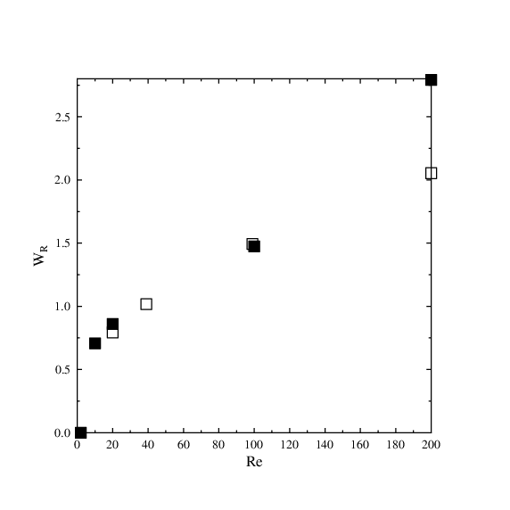
In this Section we present solutions computed for the Reynolds number spanning the range from 2 to 200. They are obtained with the resolution , , and using as the parameter of mapping (22). Filtering was performed based on exponential filer (31a) with the parameter in the range from 12 to 36. Our computational tests indicated that lower values of resulted in insufficiently accurate derivative values which made it difficult to impose Neumann boundary conditions (16d). On the other hand, larger values of resulted in spurious oscillations of the streamfunction and vorticity fields. The key parameters characterizing the solutions obtained at different Reynolds numbers are summarized in Table 2 where we also list some global diagnostic quantities typically used to characterize separated wake flows, namely, the length and half-width of the recirculation zone, separation angle and the drag coefficient where (computed in two different ways). The obtained flow patters are presented in Figure 8 in which one can see the isolines of the streamfunction and vorticity fields together with the corresponding velocity vector fields. The boundaries of the separated regions are presented in Figure 9, whereas in Figure 10 one can see the profiles of the surface vorticity as a function of the azimuthal angle . To complete the picture, in Figures 11a and 11b we present surface plots of the vorticity in the near wake region in the case of lower () and higher () Reynolds numbers. These plots illustrate the evolution of the vorticity field as the Reynolds number increases, in particular, the emergence of thin shear layers separating from the obstacle. Finally, in Figure 12 we present the dependence of diagnostic quantities , , and on the Reynolds number and compare them with the results available in the literature. We note that all the diagnostic quantities, expect for the length and half-width of the recirculation region at the highest Reynolds number, exhibit the right trends and have correct values. The discrepancies appearing at are related to insufficient numerical resolution.
| Filter | |||||||||
|---|---|---|---|---|---|---|---|---|---|
| eq. (12) | eq. (13) | ||||||||
| 2 | 64 | 100 | 1 | 12 | - | - | - | 6.6772 | 6.6930 |
| 10 | 64 | 100 | 1 | 19 | 1.4264 | 0.7506 | 40.860 | 5.8568 | 5.8412 |
| 20 | 64 | 100 | 1 | 36 | 2.0007 | 0.7722 | 44.629 | 2.2193 | 2.2124 |
| 100 | 64 | 100 | 1 | 15 | 13.062 | 1.4820 | 66.832 | 1.1255 | 1.1283 |
| 200 | 64 | 100 | 3 | 15 | 20.006 | 2.4869 | 75.079 | 0.8617 | 0.8629 |




5 Conclusions
In this study we developed and validated a computational approach to the solution of the steady 2D Navier-Stokes system in unbounded domains. The proposed method ensures that the solutions are constructed to satisfy a number of properties of such flows revealed by mathematical analysis. They concern the behavior of the velocity fields at large distances from the obstacle, more specifically, their slow decay towards the limiting values (slower than in the time-dependent case). Some related ideas were already discussed in earlier studies Fornberg (1980); Fornberg (1985); Bönisch et al. (2008a); Bönisch et al. (2005) and in recent investigation Gautier et al. (2013). Our method relies on the use of rational Chebyshev polynomials to discretize functions defined on unbounded domains, thereby avoiding the need to truncate the domain to a finite computational box. Formulation of the steady 2D Navier-Stokes flows in terms of streamfunction and vorticity results in the former field having a discontinuity at infinity. It is resolved by recasting the problem in terms of a “skeleton”, related to the corresponding Oseen flow, and suitable perturbation fields. The use of spectral discretization allows us to achieve good accuracy with modest resolutions. While we were able to obtain solutions for the Reynolds numbers spanning two orders of magnitude, computation of flows for was made difficult by the slow convergence of iterations (48). Possible reasons include poor conditioning of the algebraic system solved to determine Newton’s direction and the coupling of the drag force to the states during iterations, cf. (47). Reliable computation of steady flows for large Reynolds numbers to address the fundamental questions mentioned in the Introduction remains therefore an objective for future research. Other related open questions concern computation of steady flows in three dimensions and flows possibly involving asymmetric wakes.
Acknowledgements
The authors acknowledge the financial support from SHARCNET through a graduate scholarship and from the Natural Sciences and Engineering Research Council of Canada (NSERC) in the form of a Discovery Grant. Calculations were performed using the high-performance computing facilities provided by SHARCNET.
Appendix A Discrete Spectral Chebyshev Differentiation — Collocation Approach
We describe below the construction of differentiation matrices corresponding to the spectral Chebyshev differentiation in the collection setting. In combination with chain-rule formulas (26), they allow us to represent the derivatives with respect to the radial coordinate . The present approach is standard Canuto et al. (2007) and is described here for completeness. Given a function , the derivatives can be approximated as
| (56a) | ||||
| (56b) | ||||
where and are the collocation points defined in (24) and the entries of the first differentiation matrix are Peyret (2002)
| (57) |
where , for . The diagonal elements are calculated as proposed in Bayliss et al. (1995)
| (58) |
which is intended to improve the accuracy of the differentiation matrices by making sure that the numerical derivative of a constant function is equal to zero. Indeed, by setting in equation (56a), it is clear that the derivative vanishes at all collocations points. Discrete differentiation given in (56a) can be expressed in terms of differentiation matrix
| (59) |
The second-derivative differentiation matrix is obtained as
| (60) |
where denotes the matrix-matrix multiplication and the diagonal entries are calculated in a similar way to (58), i.e.,
| (61) |
References
References
- Allen and Southwell (1955) Allen, D. N. D. G. and Southwell, R. V. (1955). Relaxation methods applied to determine the motion, in two dimensions, of a viscous fluid past a fixed cylinder. The Quarterly Journal of Mechanics and Applied Mathematics, 8(2), 129–145.
- Anderson et al. (1999) Anderson, E., Bai, Z., Bischof, C., Blackford, S., Demmel, J., Dongarra, J., Du Croz, J., Greenbaum, A., Hammarling, S., McKenney, A., and Sorensen, D. (1999). LAPACK Users’ Guide. Society for Industrial and Applied Mathematics, Philadelphia, PA, third edition.
- Apelt (1961) Apelt, C. J. (1961). The steady flow of a viscous fluid past a circular cylinder at Reynolds numbers 40 and 44. Aeronaut. Res. Counc. Lond. R & M, 3175, 1–28.
- Batchelor (1956) Batchelor, G. K. (1956). A proposal concerning laminar wakes behind bluff bodies at large Reynolds number. Journal of Fluid Mechanics, 1(04), 388–398.
- Bayliss et al. (1995) Bayliss, A., Class, A., and Matkowsky, B. J. (1995). Roundoff error in computing derivatives using the Chebyshev differentiation matrix. Journal of Computational Physics, 116(2), 380 – 383.
- Bönisch et al. (2005) Bönisch, S., Heuveline, V., and Wittwer, P. (2005). Adaptive boundary conditions for exterior flow problems. Journal of Mathematical Fluid Mechanics, 7(1), 85–107.
- Bönisch et al. (2008a) Bönisch, S., Heuveline, V., and Wittwer, P. (2008a). Second order adaptive boundary conditions for exterior flow problems: Non–symmetric stationary flows in two dimensions. Journal of Mathematical Fluid Mechanics, 10, 45–70.
- Bönisch et al. (2008b) Bönisch, S., Heuveline, V., and Wittwer, P. (2008b). Second order adaptive boundary conditions for exterior flow problems: Non-symmetric stationary flows in two dimensions. Journal of Mathematical Fluid Mechanics, 10(1), 45–70.
- Boyd (2000) Boyd, J. B. (2000). Chebyshev and Fourier Spectral Methods. Dover, New York, U.S.A.
- Boyd (1982) Boyd, J. P. (1982). The optimization of convergence for chebyshev polynomial methods in an unbounded domain. Journal of Computational Physics, 45, 43–79.
- Breuer and Everson (1992) Breuer, K. S. and Everson, R. M. (1992). On the errors incurred calculating derivatives using Chebyshev polynomials. Journal of Computational Physics, 99(1), 56 – 67.
- Brodetsky (1923) Brodetsky, S. (1923). Discontinuous Fluid Motion Past Circular and Elliptic Cylinders. Proceedings of the Royal Society of London. Series A, 102(718), 542–553.
- Canuto et al. (2007) Canuto, C., Husaini, M. Y., Quarteroni, A., and Zang, T. A. (2007). Spectral methods: evolution to complex geometries and applications to fluid dynamics. Scientific computation. Springer.
- Chernyshenko (1988) Chernyshenko, S. I. (1988). The asymptotic form of the stationary separated circumfluence of a body at high reynolds number. Prikl. Matem. Mekh., 52, 958–966.
- Chernyshenko (1998) Chernyshenko, S. I. (1998). Asymptotic theory of global separation. Appl. Mech. Rev., 51, 523–536.
- Chernyshenko and Castro (1996) Chernyshenko, S. I. and Castro, I. P. (1996). High-Reynolds-number weakly stratified flow past an obstacle. Journal of Fluid Mechanics, 317, 155–178.
- Christov et al. (2009) Christov, C. I., Marinovab, R. S., and Marinova, T. T. (2009). Does the stationary viscous flow around a circular cylinder exist for large Reynolds numbers? a numerical solution via variational imbedding. Journal of Computational and Applied Mathematics, 226, 205–217.
- D’Alessio (1993) D’Alessio, S. J. D. (1993). Models for steady state flow past a cylinder. Ph.D. thesis, University of Western Ontario.
- Dong et al. (2014) Dong, S., Karniadakis, G., and Chryssostomidis, C. (2014). A robust and accurate outflow boundary condition for incompressible flow simulations on severely-truncated unbounded domains. Journal of Computational Physics, 261, 83–105.
- Elcrat et al. (2000) Elcrat, A., Fornberg, B., Horn, M., and Miller, K. (2000). Some steady vortex flows past a circular cylinder. Journal of Fluid Mechanics, 409, 13–27.
- Finn (1965) Finn, R. (1965). On the exterior stationary problem for the Navier–Stokes equations, and associated perturbation problems. Archive for Rational Mechanics and Analysis, 19, 363–406.
- Finn and Smith (1967a) Finn, R. and Smith, D. R. (1967a). On the linearized hydrodynamical equations in two dimensions. Archive for Rational Mechanics and Analysis, 25, 1–25.
- Finn and Smith (1967b) Finn, R. and Smith, D. R. (1967b). On the stationary solutions of the Navier-Stokes equations in two dimensions. Archive for Rational Mechanics and Analysis, 25, 26–39.
- Fornberg (1980) Fornberg, B. (1980). A numerical study of steady viscous flow past a circular cylinder. Journal of Fluid Mechanics, 98(04), 819–855.
- Fornberg (1985) Fornberg, B. (1985). Steady viscous flow past a circular cylinder up to Reynolds number 600. Journal of Computational Physics, 61(2), 297 – 320.
- Fornberg (1991) Fornberg, B. (1991). Steady incompressible flow past a row of circular cylinders. Journal of Fluid Mechanics, 225, 655–671.
- Fornberg (1993) Fornberg, B. (1993). Computing steady incompressible flows past blunt bodies — A historical overview, volume IV of Numerical Methods for Fluid Dynamics, pages 115–134. Oxford Univ. Press. (Eds.) M.J. Baines and K.W. Morton.
- Forsythe et al. (1976) Forsythe, G. E., Malcolm, M. A., and Moler, C. B. (1976). Computational Methods for Mathematical Computations. Prentice-Hall.
- Gajjar and Azzam (2004) Gajjar, J. S. B. and Azzam, N. A. (2004). Numerical solution of the Navier-Stokes equations for the flow in a cylinder cascade. Journal of Fluid Mechanics, 520, 51–82.
- Galdi (2011) Galdi, G. P. (2011). An Introduction to the Mathematical Theory of the Navier-Stokes equations. Steady State Problems. Springer, 2 edition.
- Gautier et al. (2013) Gautier, R., Biau, D., and Lamballais, E. (2013). A reference solution of the flow over a circular cylinder at . Computers & Fluids, 75, 103–111.
- Grosch and Orszag (1977) Grosch, C. E. and Orszag, S. A. (1977). Numerical solution of problems in unbounded regions: coordinate transforms. Journal of Computational Physics, 25, 273–296.
- Gustafsson (2013) Gustafsson, J. (2013). Computational Investigation of Steady Navier-Stokes Flows Past a Circular Obstacle in Two-Dimensional Unbounded Domain. Ph.D. thesis, McMaster University.
- Gustafsson and Protas (2013) Gustafsson, J. and Protas, B. (2013). On Oseen flows for large Reynolds numbers. Theoretical and Computational Fluid Dynamics, 27(5), 665–680.
- Hamielec and Raal (1969) Hamielec, A. E. and Raal, J. D. (1969). Numerical studies of viscous flow around circular cylinders. Physics of Fluids, 12(1), 11–17.
- Imai (1951) Imai, I. (1951). On the Asymptotic Behaviour of Viscous Fluid Flow at a Great Distance from a Cylindrical Body, with Special Reference to Filon’s Paradox. Proceedings of the Royal Society of London. Series A. Mathematical and Physical Sciences, 208(1095), 487–516.
- Kawaguti (1953) Kawaguti, M. (1953). Numerical solution of the Navier-Stokes equations for the flow around a circular cylinder at Reynolds number 40. Journal of the Physical Society of Japan, 8(6), 747–757.
- Keller and Takami (1966) Keller, H. B. and Takami, H. (1966). Numerical studies of viscous flow about cylinders. In Numerical Solutions of Nonlinear Differential Equations. Wiley.
- Kelley (2003) Kelley, C. T. (2003). Solving nonlinear equations with Newton’s method. Fundamentals of Algorithms. Society for Industrial and Applied Mathematics (SIAM), Philadelphia, PA.
- Kirchhoff (1869) Kirchhoff, G. (1869). Zur theorie freier flüssigkeitsstrahlen,. Journal für die reine und angewandte Mathematik (Crelles Journal), 1869(70), 289–298.
- Kreiss and Oliger (1979) Kreiss, H. and Oliger, J. (1979). Stability of the Fourier method. SIAM Journal on Numerical Analysis, 16(3), 421–433.
- Leray (1933) Leray, J. (1933). Etude de diverses èquations intègrales non linèaires et de quelques problèmes que pose l’hydrodynamique. J. Math. Pures Appl., 12, 1–82.
- Levi-Civita (1907) Levi-Civita, T. (1907). Scie e leggi di resistenza. Rendiconti del Circolo Matematico di Palermo.
- Majda et al. (1978) Majda, A., McDonough, J., and Osher, S. (1978). The Fourier method for nonsmooth initial data. Math. Comp., 32, 1041–1081.
- Nieuwstadt and Keller (1973) Nieuwstadt, F. and Keller, H. (1973). Viscous flow past circular cylinders. Computers & Fluids, 1(1), 59 – 71.
- Peyret (2002) Peyret, R. (2002). Spectral methods for incompressible viscous flow. Springer, New York, first edition.
- Protas (2011) Protas, B. (2011). On calculation of hydrodynamic forces for steady flows in unbounded domains. Journal of Fluids and Structures, 27, 1455–1460.
- Sen et al. (2009) Sen, S., Mittal, S., and Biswas, G. (2009). Steady separated flow past a circular cylinder at low Reynolds numbers. Journal of Fluid Mechanics, 620, 89–119.
- Sychev et al. (1998) Sychev, V. V., Sychev, A. I. R. V. V., and Korolev, G. L. (1998). Asymptotic Theory of Separated Flows. Cambridge University Press.
- Takami and Keller (1969) Takami, H. and Keller, H. B. (1969). Steady two-dimensional viscous flow of an incompressible fluid past a circular cylinder. Physics of Fluids, 12, 51–56.
- Thom (1933) Thom, A. (1933). The Flow Past Circular Cylinders at Low Speeds. Proceedings of the Royal Society of London. Series A, 141(845), 651–669.
- Tomotika and Aoi (1950) Tomotika, S. and Aoi, T. (1950). The steady flow of viscouis fluid past a sphere and circular cylinder at small Reynolds numbers. Q. J. Mech. Appl. Math., 3, 140–161.
- Vandeven (1991) Vandeven, H. (1991). Family of spectral filters for discontinuous problems. Journal of Scientific Computing, 6, 159–192.
- Vargas (2009) Vargas, G. A. (2009). Spectral Methods Solution Of The Navier-Stokes Equations For Steady Viscous Flows. Ph.D. thesis, Wichita State University.
- Veysey and Goldenfeld (2007) Veysey, J. and Goldenfeld, N. (2007). Simple viscous flows: From boundary layers to the renormalization group. Rev. Mod. Phys., 79(3), 883–927.
- Zebib (1987) Zebib, A. (1987). Stability of viscous flow past a circular cylinder. Journal of Engineering Mathematics, 21, 155–165.