Control Theoretic Smoothing Splines
Abstract
In this paper, we propose control theoretic smoothing splines with optimality for reducing the number of parameters that describes the fitted curve as well as removing outlier data. A control theoretic spline is a smoothing spline that is generated as an output of a given linear dynamical system. Conventional design requires exactly the same number of base functions as given data, and the result is not robust against outliers. To solve these problems, we propose to use optimality, that is, we use the norm for the regularization term and/or the empirical risk term. The optimization is described by a convex optimization, which can be efficiently solved via a numerical optimization software. A numerical example shows the effectiveness of the proposed method.
Index Terms:
Control theoretic splines, smoothing splines, optimization, convex optimization.I Introduction
The spline has been widely used in signal processing, numerical computation, statistics, etc. In particular, the smoothing spline gives a smooth curve that has the best fit to given noisy data [1, 2]. The smoothness is achieved by limiting the norm of the -th derivative of the curve as well as minimizing the squared error (or empirical risk) between data and the curve.
The control theoretic smoothing spline [3] is generalization of the smoothing spline using control theoretic ideas, by which the spline curve is determined by the output of a linear dynamical system. It is shown in [4] that control theoretic splines give a richer class of smoothing curves relative to polynomial curves. Fig. 1 illustrates the idea of the control theoretic spline; given a finite number of data, the robot modeled by a dynamical system with transfer function is driven by a control input and draws a smooth curve that fits to the data. The problem of the control theoretic spline is to find control that gives an expected motion of the robot, based on the model and the data set. Furthermore, the control theoretic spline has been proved to be useful for trajectory planning in [5], mobile robots in [6], contour modeling of images in [7], probability distribution estimation in [8], to name a few. For more applications and a rather complete theory of control theoretic splines, see [4].
Conventional design of control theoretic splines is based on optimization [3], and has two main drawbacks. One is that we need the same number of parameters as the data to represent the fitted curve. If the data set is big, then the number of parameters becomes crucial when for example the actuator system of the robot (see Fig. 1) has just a small area of memory. The other drawback is that the spline is not robust against outliers in observed data. In other words, conventional control theoretic splines are sensitive to outliers. To overcome these drawbacks, we propose to use optimality in the design. For reduction of the number of parameters, we utilize the sparsity-promoting property of the norm regularization, also known as LASSO (least absolute shrinkage and selection operator) [9, 10]. For robustness against outliers, we adopt the norm for the empirical risk minimization [11], assuming that the noise is Laplacian, heavier-tailed distribution than Gaussian that is assumed in conventional studies11 1 The idea of using a heavier-tailed loss function for control theoretic smoothing splines was first proposed in [12, 13].. The problem is then described in convex optimization, which can be efficiently solved by numerical computation software, e.g. cvx on MATLAB [14, 15]. For numerical computation, we implement the design procedure on MATLAB programs with cvx, access [16] to obtain the programs. Based on the programs, we show a numerical example that illustrates the effectiveness of the proposed method.
The remainder of this article is organized as follows: Section II reviews the conventional -optimal control theoretic spline and discusses drawbacks of the spline. Section III formulates the problem of the proposed spline to overcome drawbacks in the spline, and show a procedure to the solution. A numerical example is included in Section IV. Section V draws conclusions.

II Control Theoretic Smoothing Splines
Consider a linear dynamical system defined by
| (1) |
where , . We assume is controllable and is observable22 2 For controllability and observability of a linear system, see e.g. [17, Chap. 9].. For this system, suppose that a data set
is given, where are sampling instants which satisfy , and are noisy sampled data of the output of (1). The objective here is to find control , for the dynamical system (1) such that for . For this purpose, the following quadratic cost function has been introduced in [3]:
| (2) |
where is the regularization parameter that specifies the tradeoff between the smoothness of control defined in the first term of (2) and the minimization of the squared empirical risk in the second term. Also, is a weight for -th squared loss . Then the problem of control theoretic smoothing spline is formulated as follows:
Problem 1 ( control theoretic smoothing spline)
The optimal control that minimizes is given by [3, 4]
| (3) |
where is defined by
| (4) |
Note that in is the impulse response of the dynamical system (1). The optimal coefficients are given by
| (5) |
where
| (6) |
The matrix in (5) is the Grammian defined by
| (7) |
An advantage of the control theoretic smoothing spline is that the optimal control can be computed offline via equation (5). However, the formula indicates that if the data size is large, so is the number of base functions in , as shown in (3). This becomes a drawback if we have only a small memory or a simple actuator for drawing a curve with the optimal control . Another drawback is that the spline is not robust at all against outliers, as reported in [13], since the squared empirical risk in (2) assumes that the additive noise is Gaussian. To solve these problems, we adopt optimality for the design of spline.
III Control Theoretic Smoothing Splines
Before formulating the design problem of spline, we prove the following lemma:
Lemma 1
Assume that control is given by
| (8) |
for some , . Then we have
| (9) |
In particular, for , we have
| (10) |
Proof:
If for , then the solution of (1) is given by
Substituting (8) into the above equation gives (9). Then, from the definition of in (7), we immediately have (10). ∎
By this lemma, the error is given by
or equivalently
| (11) |
where and is given in (6). Based on this, we consider the following optimization problem:
Problem 2 (-optimal spline coefficients)
Find that minimizes
| (12) |
where and .
The regularization term, , is for sparsity of coefficients , as used in LASSO [9, 10]. Also, small leads to small norm of control since from (8) we have
for some constant . On the other hand, the empirical risk term, , is for the fidelity to the data. For , additive noise is assumed to be Laplacian, a heavy-tailed distribution, to take outliers into account, while is related to Gaussian noise. In each case, cost function is convex in .
Unlike spline, the solution to the optimization in Problem 2 cannot be represented in a closed form. However, by using a numerical optimization algorithm we can obtain an approximated solution within a reasonable time. For example, for the optimization with , we can adopt FISTA (Fast Iterative Shrinkage-Thresholding Algorithm) [18], which is an extension of Nesterov’s work [19] to achieve the convergence rate at -th iteration. On the other hand, for , there is no algorithm achieving such a rate, but the optimization is still convex and we can use an efficient convex optimization software, such as cvx on MATLAB [14, 15].
Remark 1
Remark 2
Although we have assumed that the initial state is , we can also set the initial state as a design variable in a similar manner. In this case, the output becomes
and the optimization is formulated by
| (13) |
where . This is also a convex optimization problem and can be efficiently solved via numerical optimization softwares.
Remark 3
The choice of parameters and influences the performance of curve fitting. The regularisation parameter controls the trade-off between the sparsity and fidelity of the solution; a larger leads to a sparser solution (i.e. more ’s are zero) while a smaller leads to a smaller empirical risk. On the other hand, may be chosen to be larger if the data contains smaller error. These parameters should be chosen by trial and error (e.g. cross-validation [10]).
IV Numerical Example
In this section, we show a numerical example that illustrates the effectiveness of the proposed control theoretic smoothing spline. We set the dynamical system with transfer function
State-space matrices for are given by
We assume the original curve is given by
The sampling instants are given by
that is, the data are sampled at rate [Hz] (100 samples per second) from initial time . The observed data are assumed to be disturbed by additive Laplacian noise with mean and variance . See Fig. 2 for the original curve and the observed data .
For these data, we compute the optimal coefficients of the control theoretic spline with corresponding to Laplacian noise. The design parameters are and for all (i.e. all elements have equal weight). We assume that the initial state is also a design variable, that is, we solve optimization (13).
Fig. 2 shows the resulting fitted curve computed with the -optimal control .

We can see that the data are considerably disturbed by Laplacian noise, but the reconstructed curve well fits the original curve. To see the sparsity property of the -optimal coefficients, we plot the value of the coefficients in Fig. 3.

As shown in this figure, the -optimal coefficients are quite sparse. In fact, the number of coefficients whose absolute values are greater than is just out of coefficients. On the other hand, we show the -optimal coefficients with , see equation (2), in Fig. 4.

This figure indicates that the coefficients are not sparse at all and the spline requires almost all the base functions to represent the fitted curve.
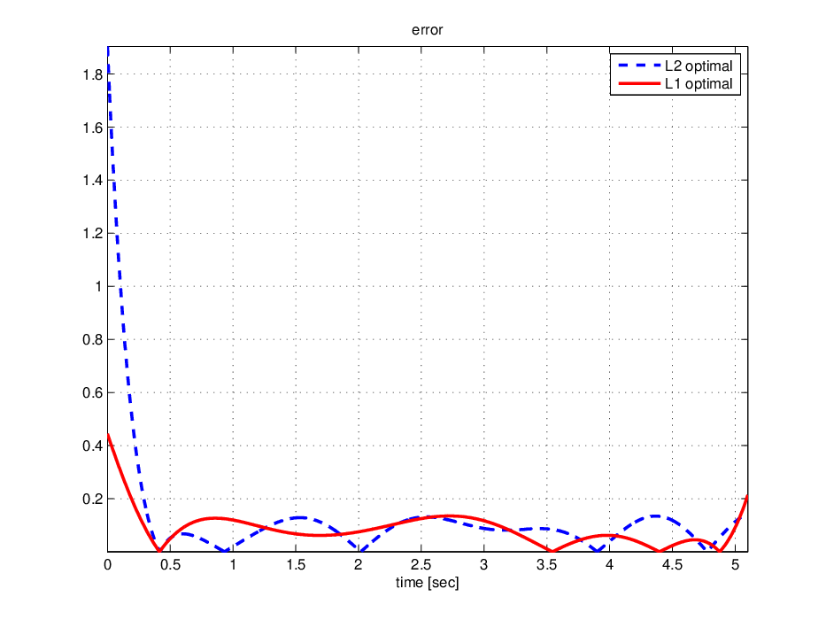
Note that the reconstructed curve by the spline also well fits the original curve as shown in Fig. 5, which shows the error between the original curve and the fitted curves. This figure shows that the spline is almost comparable with the splines33 3 Another example in [13] shows that an spline outperforms an spline in view of outlier rejection. .
In summary, we can say by the simulation that the proposed control theoretic smoothing spline can effectively reduce the effect of noise in data and also give sufficiently sparse representation for the fitted curve.
V Conclusion
In this paper, we have proposed the control theoretic smoothing splines for noise reduction and sparse representation. The design is formulated as coefficient optimization with an regularized term and an or empirical risk term, which can be efficiently solved by numerical computation softwares. A numerical example has been shown to illustrate the effectiveness of the proposed spline.
Acknowledgment
This research is supported in part by the JSPS Grant-in-Aid for Scientific Research (C) No. 24560543, MEXT Grant-in-Aid for Scientific Research on Innovative Areas No. 26120521, and an Okawa Foundation Research Grant.
References
- [1] G. Kimeldorf and G. Wahba, “Some results on Tchebycheffian spline functions,” Journal Math. Anal. Appl., vol. 33, no. 1, pp. 82–95, 1971.
- [2] G. Wahba, Spline Models for Observational Data. SIAM, 1990.
- [3] S. Sun, M. B. Egerstedt, and C. F. Martin, “Control theoretic smoothing splines,” IEEE Trans. Autom. Control, vol. 45, no. 12, pp. 2271–2279, Dec. 2000.
- [4] M. Egerstedt and C. Martin, Control Theoretic Splines. Princeton University Press, 2010.
- [5] M. Egerstedt and C. F. Martin, “Optimal trajectory planning and smoothing splines,” Automatica, vol. 37, no. 7, pp. 1057–1064, 2001.
- [6] S. Takahashi and C. F. Martin, “Optimal control theoretic splines and its application to mobile robot,” in Proc. of the 2004 IEEE CCA, 2004, pp. 1729–1732.
- [7] H. Kano, M. Egerstedt, H. Fujioka, S. Takahashi, and C. F. Martin, “Periodic smoothing splines,” Automatica, vol. 44, no. 1, pp. 185–192, 2008.
- [8] J. K. Charles, S. Sun, and C. F. Martin, “Cumulative distribution estimation via control theoretic smoothing splines,” in Three Decades of Progress in Control Sciences. Springer, 2010, pp. 83–92.
- [9] R. Tibshirani, “Regression shrinkage and selection via the LASSO,” J. R. Statist. Soc. Ser. B, vol. 58, no. 1, pp. 267–288, 1996.
- [10] P. Bühlmann and S. van de Geer, Statistics for High-Dimensional Data. Springer, 2011.
- [11] B. Schölkopf and A. J. Smola, Learning with Kernels. The MIT Press, 2002.
- [12] M. Nagahara, “Robust design of control theoretic splines via support vector regression,” in Proc. 55th Annual Conference of the Institute of Systems, Control and Information Engineers (ISCIE), 2011, (in Japanese).
- [13] M. Nagahara and C. F. Martin, “-optimal splines for outlier rejection,” in Proc. 59th World Statistics Congress, Aug. 2013, pp. 1137–1142.
- [14] M. Grant and S. Boyd, “CVX: Matlab software for disciplined convex programming, version 1.21,” http://cvxr.com/cvx, Apr. 2011.
- [15] ——, “Graph implementations for nonsmooth convex programs,” in Recent Advances in Learning and Control, ser. Lecture Notes in Control and Information Sciences, V. Blondel, S. Boyd, and H. Kimura, Eds. Splinger, 2008, vol. 371, pp. 95–110.
- [16] http://www-ics.acs.i.kyoto-u.ac.jp/mat/spline/.
- [17] W. J. Rugh, Linear Systems Theory. Prentice Hall, 1996.
- [18] A. Beck and M. Teboulle, “A fast iterative shrinkage-thresholding algorithm for linear inverse problems,” SIAM J. Imaging Sci., vol. 2, no. 1, pp. 183–202, Jan. 2009.
- [19] Y. Nesterov, “A method for unconstrained convex minimization problem with the rate of convergence ,” Doklady AN USSR, vol. 269, pp. 543–547, 1983, (translated as Soviet Math. Docl.
- [20] M. Nagahara and C. F. Martin, “Monotone smoothing splines using general linear systems,” Asian Journal of Control, vol. 5, no. 2, pp. 461–468, Mar. 2013.
- [21] M. Nagahara, D. E. Quevedo, and J. Østergaard, “Sparse packetized predictive control for networked control over erasure channels,” IEEE Trans. Autom. Control, vol. 59, no. 7, pp. 1899–1905, Jul. 2014.
- [22] M. Nagahara, D. E. Quevedo, and D. Nešić, “Maximum hands-off control and optimality,” in Proc. of 52nd IEEE Conference on Decision and Control (CDC), Dec. 2013, pp. 3825–3830.