The J-flow On Toric Manifolds

In [4], Donaldson described the various situations where the diffeomorphism groups act on some spaces of maps between manifolds, these actions induce the moment maps, then various geometric flows arise as the gradient flow of the norm square of moment maps, and the J-flow is one of these. Moreover, in the study of the K-energy, Chen [2] introduce J-flow as the gradient flow of the J-functional. Let $X$ be a Kähler manifold with a Kähler class $[\omega]$, the space of Kähler potentials is

Let $\alpha$ be a Kähler metric, the J-functional is defined on $\mathcal{H}$ by

where $\{\varphi_{t}\}_{0\leq t\leq 1}$ be any smooth path in $\mathcal{H}$ from $0$ to $\varphi$, and $c=\frac{\int\omega^{n-1}\wedge\alpha}{\int\omega^{n}}$, so $\mathcal{J}_{\alpha,\omega}(\varphi)=\mathcal{J}_{\alpha,\omega}(\varphi+a)$. The critical point $\varphi$ of $\mathcal{J}_{\alpha,\omega}$ should satisfy the Donaldson’s equation

And the J-flow is

Chen [3] showed the long time existence of J-flow and the convergence to solution of (1.1) when $\alpha$ have non-negative bisectional curvature. Then in the work of Song-Weinkove [12], by a more delicate estimate based on the previous work of Weinkove [17, 18], a necessary and sufficient condition for convergence is found,

J-flow (1.2) converges to the solution of (1.1) if and only if there exists a metric $\omega^{\prime}\in[\omega]$ such that the $(n-1,n-1)$ type form

This condition almost assume that there exists a subsolution of (1.1). However it is hard to check for concrete example. In particular, it is hard to see from this condition that whether the convergence depends on the choice of $\alpha$ in its class $[\alpha]$, in other words, if the solvability of (1.1) only depends on the class $[\omega]$ and $[\alpha]$.

In [10], Lejmi and Székelyhidi study the solvability of (1.1) from the view of geometric stability, as the problem of the existence of cscK metrics, that is conjectured be equivalent to the K-stability of manifold. Let $L$ be a line bundle on $X$, $[\omega]=c_{1}(L)$, for a test-configuration $\chi$ for $(X,L)$, they define an invariant $F_{\alpha}(\chi)$ which is similar to the Donaldson-Futaki invariant when we study the Kähler-Einstein metrics with conical singularity. It is proved that if (1.1) have a solution then $F_{\alpha}(\chi)>0$ for any test-configuration $\chi$ with positive norm, this is corresponding to the result in [14] which is for the cscK metrics. In particular, when $\chi$ is coming from the deformation to the normal cone of a subvariety (see [11]), the corresponding condition $F_{\alpha}(\chi)>0$ is

For all $p$-dimensional subvariety $V$ of $X$, where $p=1,2,\cdots,n-1$, we have

Obviously these conditions only depend on the classes. They also conjecture that (1.4) would be sufficient condition for (1.1) have solution. Moreover, (1.4) can be derived directly, suppose (1.1) have solution $\varphi$, for smooth point $x\in V$, choose coordinate $z^{i}$ such that $V=\{z^{p+1}=\cdots=z^{n}=0\}$ near $x$, and $\omega_{\varphi,i\bar{j}}=\delta_{i\bar{j}}$ at $x$, since

where $\alpha_{V}$ is the restriction of $\alpha$ on $V$. The trace $tr_{\omega_{\varphi,V}}\alpha_{V}=\sum_{i\leq p}\alpha_{i\bar{i}}<\sum\alpha_{i\bar{i}}=nc$, so $nc\omega_{\varphi,V}^{p}-p\omega_{\varphi,V}^{p-1}\wedge\alpha_{V}>0$ at $x$, then integrate it over $V_{reg}$ is (1.4). In the same way, we see $nc\omega_{\varphi}-\alpha>0$, so on the class level $nc[\omega]-[\alpha]>0$. When $n=2$, by (1.3) this is a necessary and sufficient condition for solving (1.1), but when $n>2$ it is not sufficient, see counter-example in [10].

When $n=2$, Donaldson [4] noted that the above condition $nc[\omega]-[\alpha]>0$ is satisfied for all Kähler classes if there not exist curves with negative self-intersection, and conjectured that if this condition is violated, the flow (1.2) will blow up over these curves.

In [12], they confirm the above conjecture in a partial sense. More recently, in [8, 13], they consider the situations where $nc[\omega]-[\alpha]\geq 0$ or $\alpha$ degenerate along a divisor, it is proved that the flow will converge outside a union set of curves. The argument heavily depends on the fact that when $n=2$ (1.1) can be transformed to the Monge-AmpšŠre equation, and the latter has continuous solution in the degenerate case, due to the work of Eyssidieux-Guedj-Zeriahi.

For the concrete example, Fang and Lai [7] study the long time behavior of J-flow on the projective bundles $X_{m,n}=\mathbb{P}(\mathcal{O}_{\mathbb{P}^{n}}\oplus\mathcal{O}_{\mathbb{P}^{n}}(-1)^{\oplus(m+1)})$, $X_{0,n}$ is the $\mathbb{P}^{n+1}$ blow-up one point. Under the Calabi symmetry assumption, the flow can be described by a time-dependent monotone map between two intervals, through solve the static equation (ODE), they see the flow always converges to a Kähler current and on its smooth region satisfies (1.1).

In this paper, we study J-flow on the toric manifolds and assume the metrics are invariant under torus action. We expect to find more verifiable conditions which can ensure the flow converges, maybe (1.4) for the invariant subvarieties or some combinatorial conditions for polytopes. If the flow dose not converge, we also want to understand its asymptotic behavior.

After the symmetry reduction, (1.2) can be defined on $\mathbb{R}^{n}$ by

where $\phi_{t}$ and $f$ are potentials for $\omega_{\varphi_{t}}$ and $\alpha$ respectively, they conform the asymptotic behavior at infinity assigned by the polytope $\mathcal{P}$ and $\mathcal{Q}$. Through the Legendre transform of $\phi_{t}$, this nonlinear equation be transformed to a quasilinear one which is defined on $\mathcal{P}$,

$u_{t}$ is the Legendre transform of $\phi_{t}$, satisfies Guillemin’s boundary condition, so $\nabla u_{t}$ blow up near the boundary, since $[f_{ij}]$ degenerate at infinity, so (1.5) is degenerate on the boundary, the RHS is even not defined on the boundary. Moreover, when the flow dose not converge, by the example 4.7, we see $\nabla u_{t}$ may blow up in a whole domain located in $\mathcal{P}$ as $t\rightarrow\infty$.

We turn to study the transition map $U_{t}=\nabla f\circ\nabla u_{t}$ between the moment maps induced by $\omega_{\varphi_{t}}$ and $\alpha$, it is a diffeomorphism between polytopes and map the face to face. The price is $U_{t}$ satisfies a degenerate parabolic system (4.3). The static map satisfies

In the paper we just get a partial bound on $DU_{t}$, we conjecture that $DU_{t}$ is bounded uniformly w.r.t. time, and $U_{t}$ will converge to a limit map $U_{\infty}$ even if the origin J-flow does not converge, but in this case $U_{\infty}$ must degenerate on some domain in the sense $\det DU_{\infty}=0$, since if $\det DU>\delta$ uniformly imply the flow converges. This degeneracy may violate the condition (3.6). We also want to know if J-flow minimizes the functional, namely if

where

If it does, $trDU_{\infty}$ may correspond to the worst test-configuration which be discussed in [10].

We review the Kähler structure on toric manifolds in detail, since we need the coordinate charts which include the invariant divisors, the logarithmic coordinate defined on the dense open set push these divisors to infinity. These coordinates also been introduced in [6], here we give a basis-free formulation. More details of toric variety see [9].

Let $(\mathbb{C},\times)$, $(\mathbb{R}_{\geq},\times)$ be semi-groups, $\mathbb{R}_{\geq}$ is the set of non-negative real number. $N$ is a lattice with rank $n$, its dual lattice is $M$, given a Delzant polytope $\mathcal{P}$ in $M_{R}=M\otimes_{\mathbb{Z}}\mathbb{R}$, and suppose $\{u_{i}\}\subset N$ be the prime inward normal vectors of the facets of $\mathcal{P}$, then $\mathcal{P}$ is

it induces a fan $\Sigma$ (a collection of cones) in $N_{R}=N\otimes_{\mathbb{Z}}\mathbb{R}$. For a vertex $q$ of $\mathcal{P}$, it corresponds a n-dimensional cone $\sigma_{q}$ in $\Sigma$,

its dual cone $\sigma_{q}^{\vee}=\{y\in M_{R}\mid\langle\sigma_{q},y\rangle\geq 0\}$ is generated by $\mathcal{P}-q$, and the semi-group $\sigma_{q}^{\vee}\cap M$ is finitely generated, so we can construct a finitely generated algebra $\mathbb{C}[\sigma_{q}^{\vee}\cap M]=\{\sum_{v}a_{v}\chi^{v}\mid v\in\sigma_{q}^{\vee}\cap M,\ a_{v}\in\mathbb{C}\}$ with multiplication $\chi^{v}\cdot\chi^{v^{\prime}}=\chi^{v+v^{\prime}}$, it defines an affine open set $U_{q}$

where $\varphi$ is a homomorphism between semi-groups. Let $e_{1}^{q},\cdots,e_{n}^{q}\in M$ be the prime vectors rooted at $q$ and along the edges of $\mathcal{P}$, it is a basis of $M$ due to Delzant’s conditions, and generates $\sigma_{q}^{\vee}\cap M$. Assume $\varphi(e_{i}^{q})=z_{i}^{q}$, then $U_{q}\cong\mathbb{C}^{n}=\{(z_{1}^{q},\cdots,z_{n}^{q})\}$. $U_{q}$ include the dense open subset $U_{0}=\textrm{Spm}\ \mathbb{C}[M]=\{\varphi:M\rightarrow\mathbb{C}^{*}\}\cong N\otimes_{\mathbb{Z}}\mathbb{C}^{*}\cong(\mathbb{C}^{*})^{n}$. $\{U_{q}\}$ glues with each other to form a toric manifold $X_{\Sigma}$ with a torus $\textrm{Spm}\ \mathbb{C}[M]$ action.

The subset $U_{q}^{\geq}=\{\varphi:\sigma_{q}^{\vee}\cap M\rightarrow\mathbb{R}^{\geq}\}\cong\mathbb{R}_{\geq}^{n}$ is called the non-negative part of $U_{q}$, $\pi_{q}:U_{q}\rightarrow U_{q}^{\geq}$ is defined by $\varphi\mapsto|\varphi|^{2}$. In the same way we have $\pi_{0}:U_{0}\rightarrow U_{0}^{\geq}=\{\varphi:M\rightarrow\mathbb{R}^{+}\}\cong N\otimes_{\mathbb{Z}}\mathbb{R}^{+}$. Since $(\mathbb{R}^{+},\times)\cong(\mathbb{R},+)$ by $a\mapsto\log a$, we identify $N\otimes_{\mathbb{Z}}\mathbb{R}^{+}$ with $N\otimes_{\mathbb{Z}}\mathbb{R}=N_{R}$. $\{U_{q}^{\geq}\}$ glues with each other to form a closed subset $X_{\Sigma}^{\geq}\subset X_{\Sigma}$, and $\{\pi_{q}\}$ glues to a continuous map $\pi:X_{\Sigma}\rightarrow X_{\Sigma}^{\geq}$.

Let $u$ be a symplectic potential, that is a convex function defined on $\bar{\mathcal{P}}$ and satisfies

• •

  restrict $u$ in the interior of a face, it is smooth and strictly convex.

• •

  Guillemin boundary condition, $u=\sum d_{i}(y)\log d_{i}(y)+v$, $v\in\mathcal{C^{\infty}}(\bar{\mathcal{P}})$.

Then $u$ induces an invariant Kähler metric $\omega_{u}$ in following way, let $\phi$ be the Legendre transform of $u$, which is defined on $N_{R}$, for $x\in N_{R}$,

Take a vertex $q$, let $\phi_{q}=\phi-\langle\cdot,q\rangle$, $\phi_{q}$ can be defined on $U_{0}^{\geq}$ through $U_{0}^{\geq}\cong N\otimes_{\mathbb{Z}}\mathbb{R}^{+}\cong N_{R}$. Since $U_{0}^{\geq}\subset U_{q}^{\geq}$, $\phi_{q}$ can be extended smoothly on $U_{q}^{\geq}$ due to the Guillemin’s boundary condition, denote the extension is $\bar{\phi}_{q}$. Let $\Phi_{q}=\bar{\phi}_{q}\circ\pi_{q}$, then $\omega_{q}=\frac{\sqrt{-1}}{2\pi}\partial\bar{\partial}\Phi_{q}>0$ on $U_{q}$ due to the convexity of $u$. Since $\phi_{q}-\phi_{q^{\prime}}=\langle\cdot,q^{\prime}-q\rangle$, let $\chi_{q}$ be the pullback of $\langle\cdot,q\rangle$ by the composed map $U_{0}\rightarrow U_{0}^{\geq}\rightarrow N_{R}$, so on $U_{0}$, we have $\Phi_{q}-\Phi_{q^{\prime}}=\chi_{q^{\prime}-q}$. Take a basis of $M$, $\chi_{q}$ is $(z_{1},\cdots,z_{n})\longmapsto q_{1}\log|z_{1}|^{2}+\cdots+q_{n}\log|z_{n}|^{2}$, so $\partial\bar{\partial}\chi_{q}=0$. Hence $\omega_{q}=\omega_{q^{\prime}}$ on $U_{0}$, so is on $U_{q}\cap U_{q^{\prime}}$ since $U_{0}$ is dense, so $\{\omega_{q}\}$ defines $\omega_{u}$. In another way, let $\Phi$ be the pullback of $\phi$ by $U_{0}\rightarrow U_{0}^{\geq}\rightarrow N_{R}$, then $\omega_{u}=\frac{\sqrt{-1}}{2\pi}\partial\bar{\partial}\Phi$ on $U_{0}$, and the extension of $\Phi-\chi_{q}$ to $U_{q}$ is $\Phi_{q}$.

The map $U_{0}^{\geq}\rightarrow N_{R}\stackrel{{\scriptstyle d\phi}}{{\rightarrow}}M_{R}$ can be extended to $X_{\Sigma}^{\geq}$ as a homeomorphism onto $\bar{\mathcal{P}}$, compose it with $\pi$ is the moment map $\mu$ of $(X_{\Sigma},\omega_{u})$ with respect to the torus action.

The Kähler class $[\omega_{u}]=\sum b_{i}[D_{i}]$, $D_{i}$ is the invariant divisor corresponding to $u_{i}$.

Now we take a basis of $M$ and write down the above things explicitly, let $\{e_{i}^{q}\}$ be the basis mentioned above, and the dual basis of $N$ is $\{v_{q}^{i}\}$, it is the prime generators of the cone $\sigma_{q}$.

Then $U_{q}$ have coordinates $z_{i}^{q}$, $U_{q}^{\geq}\cong\mathbb{R}_{\geq}^{n}$ have coordinates $a_{i}^{q}\geq 0$, and $U_{0}^{\geq}=\{(a_{i}^{q})\mid a_{i}^{q}>0\}$, $N_{R}$ have coordinates $x_{i}^{q}$, $M_{R}$ have coordinates $y_{q}^{i}$. The map $\pi_{q}:U_{q}\rightarrow U_{q}^{\geq}$ is $(z_{i}^{q})\mapsto(|z_{i}^{q}|^{2})$, and the identification $U_{0}^{\geq}\rightarrow N_{R}$ is $(a_{i}^{q})\mapsto(\log a_{i}^{q})$.

In the following we omit the index $q$ of variables for simplicity, $x_{i}$, $a_{i}$ always means $x_{i}^{q}$, $a_{i}^{q}$, etc.

Let

Then the Legendre transform of $u_{q}$ is $\phi_{q}(\sum x_{i}v_{q}^{i}),\ x_{i}=\partial u_{q}/\partial y^{i}$, denote it as $\phi_{q}(x_{i})\triangleq\phi_{q}(x_{1},\cdots,x_{n})$ for short. Since the map $U_{0}\rightarrow U_{0}^{\geq}\rightarrow N_{R}$ is $(z_{i})\mapsto\sum\log|z_{i}|^{2}\ v_{q}^{i}$, so $\Phi_{q}(z_{i})=\phi_{q}(\log|z_{i}|^{2})$, it can be extended smoothly on $\mathbb{C}^{n}$ as a Kähler potential, and $\bar{\phi}_{q}(a_{i})=\phi_{q}(\log a_{i})$ can be extended smoothly on $\mathbb{R}_{\geq}^{n}$. We have three functions $\Phi_{q}(z_{i})$, $(z_{i})\in\mathbb{C}^{n}$, $\bar{\phi}_{q}(a_{i})$, $(a_{i})\in\mathbb{R}_{\geq}^{n}$, $\phi_{q}(x_{i})$, $(x_{i})\in\mathbb{R}^{n}$ and satisfy

For the convexity of these functions, on $\mathbb{C}^{n}$

On $(\mathbb{C}^{*})^{n}$

$\phi_{q}$ is strictly convex on $\mathbb{R}^{n}$. For $\bar{\phi_{q}}$, note that when $z_{i}$, $z_{j}\neq 0$

we can see the RHS of (2.2) is positive definite if and only if $\bar{\phi_{q}}$ satisfies

• •

  $\frac{\partial\bar{\phi_{q}}}{\partial a_{i}}>0$ when $a_{i}=0$

• •

  for any $\Lambda\subseteq\{1,\cdots,n\}$, it can be empty, on coordinate plane $\{a_{i}>0,i\in\Lambda,a_{i}=0,i\notin\Lambda\}$,

  $$\left[\delta_{ij}a_{i}\frac{\partial\bar{\phi}_{q}}{\partial a_{i}}+a_{i}a_{j}\frac{\partial^{2}\bar{\phi_{q}}}{\partial a_{i}\partial a_{j}}\right]_{i,j\in\Lambda}>0$$

$\bar{\phi_{q}}$ and $u_{q}$ transform to each other in a way similar to the Legendre transform. For example, on coordinate plane $\{y\mid y^{n}=0,\ y^{i}\neq 0,\ i<n\}$ corresponding to the facet of polytope,

So $\bar{\phi_{q}}|_{a_{n}=0}$ is determinate by $u_{q}|_{y^{n}=0}$.

The moment map¹¹ 1 We call it as moment map just for convenient. $X_{\Sigma}^{\geq}\rightarrow\bar{\mathcal{P}}$, restrict on $U_{q}^{\geq}\cong\mathbb{R}_{\geq}^{n}$ is

it is smooth since $\bar{\phi}_{q}$ is smooth on $\mathbb{R}_{\geq}^{n}$. The inverse map is

Since $u$ satisfies the Guillemin’s boundary condition, $u_{q}=\sum y^{i}\log y^{i}+v(y)$, $v$ is smooth to the boundary, so $\exp\frac{\partial u_{q}}{\partial y^{i}}=y^{i}\exp(1+\frac{\partial v}{\partial y^{i}})$ is smooth. Hence $X_{\Sigma}^{\geq}\rightarrow\bar{\mathcal{P}}$ is actually a diffeomorphism.

On $U_{0}^{\geq}$, compose (2.5) and its inverse (2.6), we have

Take derivative w.r.t. $a_{j}$,

so on $U_{0}^{\geq}$,

with (2.2) and (2.4), $a_{i}=|z_{i}|^{2}$, we have

On the coordinate plane we have similar formula, for example on $\{z_{n}=z_{n-1}=0,\ z_{\alpha}\neq 0\}$,

We know $[u_{q,ij}]$ is singular on the boundary of polytope, however its inverse can be extended smoothly to the boundary.

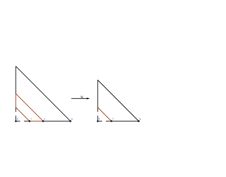
Let $\mathcal{P}$ and $\mathcal{Q}$ be defined by (2.1) with different collection of $b_{i}$, they have similar shape, for every face of $\mathcal{P}$ there is a corresponding face of $\mathcal{Q}$ parallel to it. Then induce same fan $\Sigma$, so same toric manifold $X_{\Sigma}$. Let $[\omega]$ and $[\alpha]$ be the corresponding Kähler class. The invariant Kähler metric $\omega$ induces a moment map $\mu_{\omega}:X_{\Sigma}\rightarrow\bar{\mathcal{P}}$, and $\alpha$ induces another one $\mu_{\alpha}:X_{\Sigma}\rightarrow\bar{\mathcal{Q}}$. It is well known that $\mu_{\omega}$ establishes a one-to-one correspondence between the real torus orbits and the points of $\bar{\mathcal{P}}$, so there is a transition map $U:\bar{\mathcal{P}}\rightarrow\bar{\mathcal{Q}}$ such that $U\circ\mu_{\omega}=\mu_{\alpha}$, it is a homeomorphism. We next check it is actually a diffeomorphism.

Let $u(y)$ and $g(y)$ be the symplectic potentials of $\omega$ and $\alpha$, they are defined on $\mathcal{\bar{P}}$ and $\mathcal{\bar{Q}}$ respectively. Take a vertex $q$ of $\mathcal{P}$, the corresponding vertex of $\mathcal{Q}$ is $q^{\prime}$. It corresponds an affine open set $U_{q}=U_{q^{\prime}}$, we have coordinates on it. Without loss of generality²² 2 We can translate the polytope such that $q=0$., we assume $q=q^{\prime}=0$, so $\phi=\phi_{q}$, $u=u_{q}$. In the following, we omit the index $q$, $q^{\prime}$ of potentials, and denote the potentials $\Phi$, $\bar{\phi}$, $\phi$ for $\omega$, $F$, $\bar{f}$, $f$ for $\alpha$, such that $\omega=\frac{\sqrt{-1}}{2\pi}\partial\bar{\partial}\Phi=\frac{\sqrt{-1}}{2\pi}\Phi_{i\bar{j}}dz^{i}\wedge d\bar{z}^{j}$, $\alpha=\frac{\sqrt{-1}}{2\pi}\partial\bar{\partial}F=\frac{\sqrt{-1}}{2\pi}F_{i\bar{j}}dz^{i}\wedge d\bar{z}^{j}$.

Assume

Note that $\mu_{\omega}$ is the composition of $\pi$ with $X_{\Sigma}^{\geq}\rightarrow\bar{\mathcal{P}}$, $\pi$ is independent of metrics, then compose (2.5) for $\bar{f}$ and (2.6) for $u$, we have

Since $\exp\frac{\partial u}{\partial y^{i}}=y^{i}\exp(1+\frac{\partial v}{\partial y^{i}})$ is smooth due to the Guillemin’s boundary condition, so $U$ is a diffeomorphism.

When $y^{k}>0$ for all $k$, namely in the interior of $\bar{\mathcal{P}}$, by $\bar{f}(a_{i})=f(\log a_{i})$,

namely $(U^{i})=\nabla f(\nabla u)$, since $\nabla f:\mathbb{R}^{n}\rightarrow\mathcal{Q}$ is a diffeomorphism and the inverse is $\nabla g$, so $\nabla u=\nabla g(U)$. Change the order of derivatives, $u_{ij}=u_{ji}$, we see $U$ must satisfy a compatible condition,

by Proposition 2.1, $g^{ik}$ is smooth on $\mathcal{\bar{Q}}$, so above identity is actually valid on $\mathcal{\bar{P}}$.

For metric $\omega$ and $\alpha$, we defined a linear transform $A$ on $T^{1,0}X$ by

where $\langle\partial_{i},\partial_{j}\rangle_{\omega}=\Phi_{i\bar{j}}$. Suppose $A\partial_{i}=A_{i}^{k}\partial_{k}$, then $A_{i}^{k}=F_{i\bar{j}}\Phi^{k\bar{j}}$. $A$ is self-dual respect to $\omega$ and $\alpha$, namely $\langle A\partial_{i},\partial_{j}\rangle_{\omega}=\langle\partial_{i},A\partial_{j}\rangle_{\omega}$, $\langle A\partial_{i},\partial_{j}\rangle_{\alpha}=\langle\partial_{i},A\partial_{j}\rangle_{\alpha}$, and positive $\langle Ax,x\rangle_{\omega}=\langle x,x\rangle_{\alpha}>0$ for $0\neq x\in T^{1,0}M$.

On $U_{0}\cong(\mathbb{C}^{*})^{n}$, by (2.3) and (2.8),

The characteristic polynomial of $A:T^{1,0}M\rightarrow T^{1,0}M$

This identity holds on $X$ by continuation.

Note that

so we have

In particular,

Donaldson’s equation (1.1) is $trDU\equiv nc$, and $U$ is subject to (3.2).

Moreover, when we restrict metrics on the invariant subvariety, we have

In particular, on $V$

Note that the push-out measure of $\frac{\omega_{V}^{p}}{p!}$ by $\mu_{\omega}|_{V}$ is $\sigma_{F}$, the canonical measure on $F$. First we have the Lebesgue measure $\Omega$ on $M_{R}$ induced by the lattice $M$, and let $\{u_{i}\}_{i=1}^{n-p}$ be the generators that vanished along $TF$, then $\sigma_{F}=(\iota_{v_{1}}\cdots\iota_{v_{n-p}}\Omega)|_{TF}$, where $\{v_{i}\}\subset M_{R}$ such that $\langle u_{i},v_{j}\rangle=\delta_{ij}$. Integrate (3.5), we have

References

[1]Chen, B. H., Li, A. M., Sheng, L.: Extremal
metrics on toric surfaces. arXiv:1008.2607, 2010.
[2]Chen, X. X.: On the lower bound of the Mabuchi
energy and its application. Int. Math. Res. Notices 12 (2000), 607–623.
[3]——: A new parabolic
flow in Kähler manifolds. Comm. Anal. Geom. 12, no.4 (2004), 837–852.
[4]Donaldson, S. K.: Moment maps and diffeomorphisms.
Asian J. Math. 3, no. 1 (1999), 1–16.
[5]——:
Scalar curvature and stability of toric varieties. Journal of Differential
Geometry, 2002, 62(2): 289-349.
[6]——: Constant scalar
curvature metrics on toric surfaces. Geometric and Functional Analysis,
2009, 19(1): 83-136.
[7]Fang, H., Lai, M. J.: Convergence of general inverse
-flow on Kähler manifolds with Calabi ansatz. Transactions
of the American Mathematical Society, 2013, 365(12): 6543-6567.
[8]Fang, H., Lai, M. J., Song, J., Weinkove, B.: The
J-flow on Kähler surfaces: a boundary case. Analysis & PDE, 2014,
7(1): 215-226.
[9]Fulton, W.: Introduction to toric varieties, Princeton
University Press, 1993.
[10]Lejmi, M., Székelyhidi, G.: The J-flow and
stability. arXiv:1309.2821, 2013.
[11]Ross, J., Thomas, R.: An obstruction
to the existence of constant scalar curvature Kähler metrics. Journal
of Differential Geometry, 2006, 72(3): 429-466.
[12]Song, J., Weinkove, B.: The convergence and singularities
of the J-flow with applications to the Mabuchi energy. Comm. Pure
Appl. Math. 61 (2008), no. 2, 210–229.
[13]——: The Degenerate J-flow
and the Mabuchi energy on minimal surfaces of general type. Universitatis
Iagellonicae Acta Mathematica, 2014, 50.
[14]Székelyhidi, G.: Filtrations and test-configurations.
arXiv:1111.4986, 2011.
[15]Tian, G.: Canonical metrics in Kähler geometry,
Springer, 2000.
[16]Wang, X. J., Zhu, X. H.: Kähler–Ricci
solitons on toric manifolds with positive first Chern class. Advances
in Mathematics, 2004, 188(1): 87-103.
[17]Weinkove, B.: Convergence of the J -flow on Kähler
surfaces, Comm. Anal. Geom. 12, no. 4 (2004), 949–965.
[18]——: On the J-flow in higher
dimensions and the lower boundedness of the Mabuchi energy, J. Differential
Geom. 73 (2006), no. 2, 351–358.