跳到论文正文
W Papers独立论文阅读器 arXiv:1407.0912 论文正文 计算阅读时间 · 0%
引用这篇论文根据当前论文元数据生成,正式投稿前建议核对。


License: arXiv.org perpetual non-exclusive license
arXiv:1407.0912v3 [math.AP] 08 Apr 2015

Unfolding operator method for thin domains with a locally periodic highly oscillatory boundary

This research has been partially supported by grant MTM2012-31298, MINECO, Spain and Grupo de Investigación CADEDIF, UCM. The second author, Manuel Villanueva-Pesqueira, also partially supported by a FPU fellowship (AP2010-0786) from the Goverment of Spain.
José M. Arrieta Note: Departamento de Matemática Aplicada, Universidad Complutense de Madrid, 28040 Madrid and Instituto de Ciencias Matemáticas CSIC-UAM-UC3M-UCM, C/Nicolás Cabrera 13-15, Cantoblanco, 28049 Madrid, Spain    Manuel Villanueva-Pesqueira Note: Departamento de Matemática Aplicada, Universidad Complutense de Madrid, 28040 Madrid, Spain

Abstract : We analyze the behavior of solutions of the Poisson equation with homogeneous Neumann boundary conditions in a two-dimensional thin domain which presents locally periodic oscillations at the boundary. The oscillations are such that both the amplitude and period of the oscillations may vary in space. We obtain the homogenized limit problem and a corrector result by extending the unfolding operator method to the case of locally periodic media. We emphasize the fact that the techniques developed in this paper can be adapted to other locally periodic cases like reticulated or perforated domains where the period may be space-dependent.

Keywords : Thin domain ; oscillatory boundary ; homogenization ; unfolding method ; locally periodic ; varying period

2000 Mathematics Subject Classification : 35B27, 74K10, 74Q05

1 Introduction

In this paper we study the behavior of the solutions of the Neumann problem for the Laplace operator

{−Δ​uϵ+uϵ=fϵ in ​Rϵ∂uϵ∂νϵ=0 on ​∂Rϵ\left\{\begin{gathered}-\Delta u^{\epsilon}+u^{\epsilon}=f^{\epsilon}\quad\textrm{ in }R^{\epsilon}\\ \frac{\partial u^{\epsilon}}{\partial\nu^{\epsilon}}=0\quad\textrm{ on }\partial R^{\epsilon}\end{gathered}\right. (1.1)

where fϵ∈L2​(Rϵ)f^{\epsilon}\in L^{2}(R^{\epsilon}), νϵ=(ν1ϵ,ν2ϵ)\nu^{\epsilon}=(\nu^{\epsilon}_{1},\nu^{\epsilon}_{2}) is the unit outward normal to ∂Rϵ\partial R^{\epsilon} and ∂∂νϵ\frac{\partial}{\partial\nu^{\epsilon}} is the outside normal derivative. The domain RϵR^{\epsilon} is a two dimensional thin domain which presents a highly oscillatory behavior at the top boundary, given by

Rϵ={(x,y)∈ℝ2|x∈(0,1)​, 0<y<ϵ​G​(x,x/ϵ)}R^{\epsilon}=\{(x,y)\in\mathbb{R}^{2}\;|\;x\in(0,1),\,0<y<\epsilon\,G(x,x/\epsilon)\} (1.2)

where the smooth function GG, defined as

G:(0,1)×ℝ⟶(0,+∞)(x,y)⟶G⁡(x,y)\begin{array}[]{rl}G:(0,1)\times\mathbb{R}&\longrightarrow(0,+\infty)\\ (x,y)&\longrightarrow G(x,y)\end{array}

satisfies that there exist two positive constants G0G_{0}, G1G_{1} with

0<G0≤G(x,y)≤G1,∀(x,y)∈(0,1)×ℝ.\begin{gathered}0<G_{0}\leq G(x,y)\leq G_{1},\quad\forall(x,y)\in(0,1)\times\mathbb{R}.\end{gathered}

Moreover, for each x∈(0,1)x\in(0,1), the function G⁡(x,⋅)G(x,\cdot) is l⁡(x)l(x)-periodic, with the function l⁡(⋅)l(\cdot) not being necessarily constant. This includes the case where the thin domain is locally periodic with constant period, for instance, G⁡(x,x/ϵ)=a⁡(x)+b⁡(x)​g​(x/ϵ)G(x,x/\epsilon)=a(x)+b(x)g(x/\epsilon) where a,b:(0,1)→ℝa,b:(0,1)\to\mathbb{R} are 𝒞1\mathcal{C}^{1} functions and g:ℝ→ℝg:\mathbb{R}\to\mathbb{R} is an L-periodic smooth function (see for instance [5]). But, it also includes the very important and relevant case where the period changes as we vary xx. For instance, G⁡(x,x/ϵ)=a⁡(x)+b⁡(x)​g​(l⁡(x)​x/ϵ)G(x,x/\epsilon)=a(x)+b(x)g(l(x)x/\epsilon) where l:ℝ→ℝl:\mathbb{R}\to\mathbb{R} is certain smooth function.

Refer to caption
Figure 1: Model thin domain RϵR^{\epsilon}

The main novelty in this work is that we consider domains where both the amplitude and frequency of the oscillations depend on xx (see Figure 1). In this respect we are deviating from the purely periodic case, which is the most common setting in homogenization theory and we are interested in analyzing how the geometry of the domain, the varying amplitude and period of the function GG, affects the homogenized limit problem.

The purely periodic case can be addressed by somehow standard techniques in homogenization theory, as developed in [9, 17, 36, 21]. If Gϵ​(x)=G⁡(x/ϵ)G_{\epsilon}(x)=G(x/\epsilon) where GG is an LL-periodic C1C^{1} function and if we denote by

Y∗={(y1,y2)∈ℝ2: 0<y1<L,0<y2<G(y1)}Y^{*}=\{(y_{1},y_{2})\in\mathbb{R}^{2}\;:\;0<y_{1}<L,\quad 0<y_{2}<G(y_{1})\}

then the limit equation is shown to be

{−q0​wx​x+w=f⁡(x),x∈(0,1)w′​(0)=w′​(1)=0\left\{\begin{gathered}-q_{0}w_{xx}+w=f(x),\quad x\in(0,1)\\ w^{\prime}(0)=w^{\prime}(1)=0\end{gathered}\right. (1.3)

where

q0=1|Y∗|​∫Y∗{1−∂X∂y1​(y1,y2)}​d​y1​d​y2,\begin{gathered}q_{0}=\frac{1}{|Y^{*}|}\int_{Y^{*}}\Big\{1-\frac{\partial X}{\partial y_{1}}(y_{1},y_{2})\Big\}dy_{1}dy_{2},\qquad\end{gathered}

and XX is the unique solution of certain PDE problem posed in the basic cell Y∗Y^{*}. We refer to [31, 5, 4] for details.

Also, the case where the function G⁡(x,⋅)G(x,\cdot) is LL-periodic with LL independent of xx, that is, locally periodic case with fixed period, was analyzed in [5]. With the method of oscillatory test functions applied first to the case of piecewise periodic case and then with a domain perturbation argument, the following limit problem was obtained:

{−1p⁡(x)​(q⁡(x)​wx)x+w=f⁡(x),x∈(0,1)w′​(0)=w′​(1)=0\left\{\begin{gathered}-\frac{1}{p(x)}(q(x)w_{x})_{x}+w=f(x),\quad x\in(0,1)\\ w^{\prime}(0)=w^{\prime}(1)=0\end{gathered}\right. (1.4)

where

q⁡(x)=∫Y∗​(x){1−∂X⁡(x)∂y1​(y1,y2)}​d​y1​d​y2,\begin{gathered}q(x)=\int_{Y^{*}(x)}\Big\{1-\frac{\partial X(x)}{\partial y_{1}}(y_{1},y_{2})\Big\}dy_{1}dy_{2},\qquad\end{gathered} (1.5)
p​(x)=|Y∗​(x)|p(x)=|Y^{*}(x)| (1.6)

and X​(x)​(⋅,⋅)X(x)(\cdot,\cdot) is the unique solution of an appropriate PDE problem posed in the basic cell Y∗​(x)Y^{*}(x) which depends on the variable xx and it is given by

Y∗(x)={(y1,y2)∈ℝ2: 0<y1<L,0<y2<G(x,y1)}.Y^{*}(x)=\{(y_{1},y_{2})\in\mathbb{R}^{2}\;:\;0<y_{1}<L,\quad 0<y_{2}<G(x,y_{1})\}.

Notice that if we assume that Y∗​(x)≡Y∗Y^{*}(x)\equiv Y^{*}, then we recover the homogenized problem in the purely periodic case.

The analysis performed in [5] used in a very definite way that the period of the function G⁡(x,⋅)G(x,\cdot) is independent of xx and the techniques do not apply in a very straightforward way to the more general case of a varying period.

In the literature there are several, although not many, works on homegenization in locally periodic structures. In [13, 32, 33] an asymptotic expansion technique was used to obtain the limit problem and the estimates of the rate of the convergence for problems defined in domains with locally periodic perforations, i.e. the geometry of the cavities varies with space. Two scale convergence was applied in [14, 30] to homogenize the warping, the torsion and the Neumann problems in two dimensional domains with smoothy changing holes and in [29] two scale convergence was generalized to a locally periodic and fibrous media. All these works deal with the case where the basic cell varies with space but the period in which the basic cell is spaced is constant and do not vary with space.

Let us also point out that there are several papers addressing the problem of studying the effect of rough boundaries on the behavior of the solution of partial differential equations. Among others, we can mention [1, 10, 12, 24, 27, 28] in the context of fluid flows and [15, 16] where complete asymptotic expansions of the solutions were studied.

When dealing with a thin domain RϵR^{\epsilon} as defined in (1.2), where the function G⁡(x,⋅)G(x,\cdot) is periodic of period l⁡(x)l(x), we may distinguish two different situations.

On one hand, if the function h⁡(x)=xl⁡(x)h(x)=\frac{x}{l(x)} satisfies h′​(x)>0h^{\prime}(x)>0 for all x∈[0,1]x\in[0,1] then h:(0,1)→(0,1l⁡(1))h:(0,1)\to\Big(0,\frac{1}{l(1)}\Big) is a diffeomorphism. In this particular case, if seems reasonable to perform the following change of variables

Zϵ:Rϵ⟶R1ϵ(x,y)⟶(x1,x2):=(h⁡(x),y)=(xl⁡(x),y).\begin{array}[]{rl}Z^{\epsilon}:R^{\epsilon}&\longrightarrow R_{1}^{\epsilon}\\ (x,y)&\longrightarrow(x_{1},x_{2}):=\big(h(x),y\big)=\Big(\frac{x}{l(x)},y\Big).\end{array}

which transforms the thin domain RϵR^{\epsilon} into another thin domain, R1ϵR_{1}^{\epsilon}, having an oscillatory boundary given by the 1−1-periodic function H⁡(x,y)=G⁡(h−1​(x),l⁡(h−1​(x))​y)H(x,y)=G(h^{-1}(x),l(h^{-1}(x))y), that is

R1ϵ={(x1,x2)∈ℝ2|x1∈(0,1/l⁡(1))​, 0<x2<ϵ​H​(x1,x1/ϵ)}.R_{1}^{\epsilon}=\Big\{(x_{1},x_{2})\in\mathbb{R}^{2}\;|\;x_{1}\in(0,1/l(1)),\;0<x_{2}<\epsilon\,H(x_{1},x_{1}/\epsilon)\Big\}.

In this new system of coordinates, problem (1.1) is transformed into

{−h′​(h−1​(x1))​div​(B⁡(vϵ))+vϵ=fϵ in ​R1ϵ,B⁡(vϵ)⋅η=0 on ​∂R1ϵ,vϵ=uϵ∘(Zϵ)−1​ in ​R1ϵ\left\{\begin{gathered}-h^{\prime}(h^{-1}(x_{1}))\hbox{div}\big(B(v^{\epsilon})\big)+v^{\epsilon}=f^{\epsilon}\quad\textrm{ in }R_{1}^{\epsilon},\\ B(v^{\epsilon})\cdot\eta=0\quad\textrm{ on }\partial R_{1}^{\epsilon},\\ v^{\epsilon}=u^{\epsilon}\circ(Z^{\epsilon})^{-1}\textrm{ in }R_{1}^{\epsilon}\end{gathered}\right. (1.7)

where η\eta denotes the unit outward normal vector field to ∂R1ϵ\partial R_{1}^{\epsilon} and

B⁡(v)=(h′​(h−1​(x1))​∂v∂x1,1h′​(h−1​(x1))​∂v∂x2).B(v)=\Big(h^{\prime}(h^{-1}(x_{1}))\frac{\partial v}{\partial x_{1}},\frac{1}{h^{\prime}(h^{-1}(x_{1}))}\frac{\partial v}{\partial x_{2}}\Big).

Under this change of variables, we have transformed the thin domain with variable amplitude and period of the oscillations into a locally periodic thin domain with constant period, although the amplitude continues to vary with space (that is, the function H⁡(x,y)H(x,y) actually depends on xx). Moreover, in this case, the transformed differential operator, see (1.7), is now with non-constant coefficients. Now, we may proceed using the techniques from [5] or try to use the unfolding operator method adapted to the situation of variable amplitude, which is a particular case of what we are developing in this paper.

On the other hand, if the function h⁡(x)=xl⁡(x)h(x)=\frac{x}{l(x)} is not a diffeomorphism, we cannot perform this changes of variables. This is the situation that we are considering in this paper. As a matter of fact we will assume the following hypothesis

  • (H)

    The function l⁡(⋅)l(\cdot) is 𝒞1\mathcal{C}^{1} and there exist positive constants l0,l1l_{0},l_{1} such that 0<l0⩽l⁡(x)<l10<l_{0}\leqslant l(x)<l_{1}. Moreover, for all k∈ℝk\in\mathbb{R} the points x∈(0,1)x\in(0,1) such that x=k​l​(x)x=kl(x) is a finite set and if A={x∈(0,1):x​l′​(x)=l⁡(x)}A=\{x\in(0,1):xl^{\prime}(x)=l(x)\}, then μ​{A}=0\mu\{A\}=0, where μ\mu denotes the Lebesgue measure.

This hypothesis contemplates the possibility that hh has a finite number of maxima and minima (see for instance Figure 2) or even the more degenerate situation where the function h⁡(x)h(x) has an infinite number of critical points (see Figure 3). For both cases, it does not seem possible to perform a change of variables that transform the problem in a domain with fixed period.

Refer to caption
(a) Function h⁡(x)=xl⁡(x)h(x)=\frac{x}{l(x)}
Refer to caption
(b) Corresponding thin domain
Figure 2: AA is a finite set.
Refer to caption
(a) Function h⁡(x)=xl⁡(x)h(x)=\frac{x}{l(x)}
Refer to caption
(b) Corresponding thin domain
Figure 3: AA is a infinite numerable set.

Our proposal consist in avoiding to make a change of variables and rather adapt the Unfolding Operator method, which was initially devised to tackle purely periodic problems, to this new “locally periodic” situation. We refer to [3, 11] for the first descriptions of the unfolding operator method, [19, 20] for a systematic treatment of this method and [22] for an application of the method to a 2-dimensional domain with oscillating boundaries (actually [22] is the first time where the unfolding operator method is applied to a domain with an oscillatory boundary).

Let us mention that this adjustment of the method applies also to the case where the period does not depend on the spatial variable xx and we may consider this as a different method to obtain the results from [5]. Moreover, the possibility to apply the unfolding operator method to a non-periodic situation express the robustness and power of the method.

Our results, which were announced in [8] for the simpler and more intuitive case where h′​(⋅)>0h^{\prime}(\cdot)>0, will allow us to obtain the homogenized limit problem, together with a corrector result, for problems defined on thin domains with locally-periodic oscillatory boundary. This extension is performed for the case of thin domains, but the ideas and techniques can be applied to other situations like perforated domains where both hole and periodicity of the cell vary smoothly. We will deal with this more general situation in a future publication. As a matter of fact, the limit problem we obtain is:

{−l⁡(x)|Y∗​(x)|​(r⁡(x)​ux)x+u=f,x∈(0,1)u′​(0)=u′​(1)=0\left\{\begin{gathered}-\frac{l(x)}{|Y^{*}(x)|}\big(r(x)u_{x}\big)_{x}+u=f,\quad x\in(0,1)\\ u^{\prime}(0)=u^{\prime}(1)=0\end{gathered}\right.

with

r⁡(x)=1l⁡(x)​∫Y∗​(x){1−∂X⁡(x)∂y1​(y1,y2)}​d​y1​d​y2r(x)=\frac{1}{l(x)}\int_{Y^{*}(x)}\Big\{1-\frac{\partial X(x)}{\partial y_{1}}(y_{1},y_{2})\Big\}dy_{1}dy_{2}

where Y∗​(x)Y^{*}(x) is the basic cell given by

Y∗(x)={(y1,y2)∈ℝ2: 0<y1<l(x),0<y2<G(x,y1)},Y^{*}(x)=\{(y_{1},y_{2})\in\mathbb{R}^{2}\;:\;0<y_{1}<l(x),\quad 0<y_{2}<G(x,y_{1})\},

and X​(x)​(⋅,⋅)X(x)(\cdot,\cdot) is the unique solution of an appropriate PDE problem posed in the basic cell Y∗​(x)Y^{*}(x). Notice that if l⁡(x)l(x) is a constant independent of x∈(0,1)x\in(0,1) we recover (1.4), (1.5), (1.6).

The paper is organized as follow. In Section 2, we fix some notation that will be used throughout the paper. In 3 we construct the unfolding operator for locally periodic thin domains and show some important properties. In Section 4, we present some convergence results related to the unfolding operator. The essential result for the work is the compactness Theorem 4.11. In Section 5, we apply the previous results to obtain the homogenized limit problem. The Theorem 5.1 shows two equivalent formulations of the homogenized limit problem. Finally, in Section 6, we introduce an averaging operator 𝒰ϵ\mathcal{U}_{\epsilon} , the adjoint of the unfolding operator, and we prove its main properties. To end the paper, we use the averaging operator to obtain a corrector result.

Acknowledgment. The authors are grateful to G. Griso, A. Damlamian and P. Donato for helpful comments and suggestions.

2 Some notation

Before embarking into the statements and proofs of the results let us clarify some notation that we will use throughout the article.

i) Observe that properly speaking there is not a basic cell associated to the domain RϵR^{\epsilon}, since the periodicity properties vary from point to point in x∈(0,1)x\in(0,1). Nevertheless, we will refer to the set Y∗​(x)Y^{*}(x) defined by

Y∗(x)={(y1,y2)∈ℝ2: 0<y1<l(x),0<y2<G(x,y1)}.Y^{*}(x)=\{(y_{1},y_{2})\in\mathbb{R}^{2}\;:\;0<y_{1}<l(x),\quad 0<y_{2}<G(x,y_{1})\}. (2.1)

as the basic cell at xx. Notice that all these “basic cells” satisfy Y∗​(x)⊂Y∗Y^{*}(x)\subset Y^{*} where Y∗=(0,l1)×(0,G1)Y^{*}=(0,l_{1})\times(0,G_{1}).

ii) The basic idea of the unfolding operator method in a purely periodic setting is to transform functions defined in RϵR^{\epsilon} into functions defined in a fixed domain. With analogy to this case, we will consider the domain

W={(x,y1,y2)∈ℝ3:x∈(0,1),(y1,y2)∈Y∗(x)}W=\{(x,y_{1},y_{2})\in\mathbb{R}^{3}\,:\;x\in(0,1),\;(y_{1},y_{2})\in Y^{*}(x)\}

and W^={(x,y1,y2)∈ℝ3:x∈(0,1),y1∈ℝ\hat{W}=\{(x,y_{1},y_{2})\in\mathbb{R}^{3}\,:\;x\in(0,1),\;y_{1}\in\mathbb{R} and 0<y2<G(x,y1)}0<y_{2}<G(x,y_{1})\}. Notice that W={(x,y1,y2)∈W^:0<y1<l⁡(x)}W=\{(x,y_{1},y_{2})\in\hat{W}:0<y_{1}<l(x)\} and W⊂(0,1)×Y∗W\subset(0,1)\times Y^{*}. Moreover, W0={(x,y1)∈ℝ2:x∈(0,1),y1∈(0,l(x)}.W_{0}=\{(x,y_{1})\in\mathbb{R}^{2}:\;x\in(0,1),\;y_{1}\in(0,l(x)\}. Observe that this set is the bottom boundary of WW.

iii) Given an interval (a,b)⊂ℝ(a,b)\subset\mathbb{R} we denote its characteristic function by χ(a,b)\chi_{(a,b)}. χϵ\chi^{\epsilon} is the characteristic function of RϵR^{\epsilon} and χ\chi the characteristic function of WW. Moreover, as it is usually done, ~\,\widetilde{}\; is the standard extension by zero operator.

iv) We will use the subindex #\# to denote periodicity with respect to the y1y_{1} variable in the following sense. For every fixed x∈(0,1)x\in(0,1), the space C#k​(Y∗​(x))C^{k}_{\#}\big(Y^{*}(x)\big) consists of all functions φ\varphi which are obtained as restrictions to Y∗​(x)Y^{*}(x) of functions in Ck​(ℝ2)C^{k}(\mathbb{R}^{2}) which are l⁡(x)l(x)-periodic in the first variable. That is

C#k(Y∗(x))={φ|Y∗(x):φ∈Ck(ℝ2),φ(y1+l(x),y2)=φ(y1,y2),∀(y1,y2)∈ℝ2}.C^{k}_{\#}\big(Y^{*}(x)\big)=\{\varphi_{|Y^{*}(x)}:\varphi\in C^{k}(\mathbb{R}^{2}),\,\varphi(y_{1}+l(x),y_{2})=\varphi(y_{1},y_{2}),\quad\forall(y_{1},y_{2})\in\mathbb{R}^{2}\}.

This is a Banach space with the usual norm ∥⋅∥Ck​(Y∗​(x))\|\cdot\|_{C^{k}(Y^{*}(x))}.

Also, W#1,p​(Y∗​(x))W^{1,p}_{\#}\big(Y^{*}(x)\big) is the completion for the norm of W1,p​(Y∗​(x))W^{1,p}\big(Y^{*}(x)\big) of C#∞​(Y∗​(x))C^{\infty}_{\#}\big(Y^{*}(x)\big). Moreover, the space C#∞​(W)C^{\infty}_{\#}(W) is the space of functions which are restrictions to WW of functions φ∈C∞​(ℝ3)\varphi\in C^{\infty}(\mathbb{R}^{3}) which for fixed x∈(0,1)x\in(0,1) they are periodic in the y1y_{1} variable of period l⁡(x)l(x), that is: φ⁡(x,y1+l⁡(x),y2)=φ⁡(x,y1,y2)\varphi(x,y_{1}+l(x),y_{2})=\varphi(x,y_{1},y_{2}).

v) We define the spaces of Banach space-valued functions Lp​((0,1),W#1,q​(Y∗​(x)))L^{p}\Big((0,1);W^{1,q}_{\#}\big(Y^{*}(x)\big)\Big),
Lp​((0,1),C#k​(Y∗​(x)))L^{p}\Big((0,1);C^{k}_{\#}\big({Y^{*}(x)}\big)\Big) and W1,p​((0,1),C#k​(Y∗​(x)))W^{1,p}\Big((0,1);C^{k}_{\#}\big({Y^{*}(x)}\big)\Big) in the following way:

  • (1)

    The space Lp​((0,1),W#1,q​(Y∗​(x)))L^{p}\Big((0,1);W^{1,q}_{\#}\big(Y^{*}(x)\big)\Big) consists of the measurable functions φ:W→ℝ\varphi:W\to\mathbb{R} such that φ⁡(x)∈W#1,q​(Y∗​(x))\varphi(x)\in W^{1,q}_{\#}\big(Y^{*}(x)\big) a.e. x∈(0,1)x\in(0,1), with

    ∥φ∥Lp​((0,1),W#1,q​(Y∗​(x))):={(∫01‖φ⁡(x)‖W#1,q​(Y∗​(x))p​dx)1/p<∞, for ​1≤p<∞ess​supx∈(0,1)∥φ(x)∥W#1,q​(Y∗​(x))<∞, for p=∞.\|\varphi\|_{L^{p}\Big((0,1);W^{1,q}_{\#}\big(Y^{*}(x)\big)\Big)}:=\left\{\begin{gathered}\Big(\int_{0}^{1}\|\varphi(x)\|^{p}_{W^{1,q}_{\#}\big(Y^{*}(x)\big)}\;dx\Big)^{1/p}<\infty,\hbox{ for }1\leq p<\infty\\ \operatorname*{ess\,sup}_{x\in(0,1)}\|\varphi(x)\|_{W^{1,q}_{\#}\big(Y^{*}(x)\big)}<\infty,\hskip 8.5359pt\hbox{ for }p=\infty.\end{gathered}\right.

    Notice that L2​((0,1),H#1​(Y∗​(x)))L^{2}\Big((0,1);H^{1}_{\#}\big(Y^{*}(x)\big)\Big) actually coincides with the space of functions φ∈L2​(W)\varphi\in L^{2}(W) such that ∂φ∂y1\frac{\partial\varphi}{\partial y_{1}}, ∂φ∂y2\frac{\partial\varphi}{\partial y_{2}} belong to L2​(W)L^{2}(W) and φ⁡(x,⋅,⋅)\varphi(x,\cdot,\cdot) is l⁡(x)l(x)-periodic in the first variable y1y_{1}.

  • (2)

    The space Lp​((0,1),C#k​(Y∗​(x)))L^{p}\Big((0,1);C^{k}_{\#}\big({Y^{*}(x)}\big)\Big) comprises all strongly measurable functions φ:W→ℝ\varphi:W\to\mathbb{R} such that φ⁡(x)∈C#k​(Y∗​(x))\varphi(x)\in C^{k}_{\#}\big(\;{Y^{*}(x)}\;\big) and

    ∥φ∥Lp​((0,1),C#k​(Y∗​(x))):={(∫01‖φ⁡(x)‖C#k​(Y∗​(x))p​dx)1/p<∞, for ​1≤p<∞ess​supx∈(0,1)∥φ(x)∥C#k​(Y∗​(x))<∞, for p=∞.\|\varphi\|_{L^{p}\Big((0,1);C^{k}_{\#}\big(\,{Y^{*}(x)}\,\big)\Big)}:=\left\{\begin{gathered}\Big(\int_{0}^{1}\|\varphi(x)\|^{p}_{C^{k}_{\#}\big({Y^{*}(x)}\big)}\;dx\Big)^{1/p}<\infty,\hbox{ for }1\leq p<\infty\\ \operatorname*{ess\,sup}_{x\in(0,1)}\|\varphi(x)\|_{C^{k}_{\#}\big({Y^{*}(x)}\big)}<\infty,\hskip 8.5359pt\hbox{ for }p=\infty.\end{gathered}\right.
  • (3)

    The space W1,p​((0,1),C#k​(Y∗​(x)))W^{1,p}\Big((0,1);C^{k}_{\#}\big(\,{Y^{*}(x)}\,\big)\Big) consists of all functions φ∈Lp​((0,1),C#k​(Y∗​(x)))\varphi\in L^{p}\Big((0,1);C^{k}_{\#}\big(\,{Y^{*}(x)}\,\big)\Big) such that ∂xφ\partial_{x}\varphi exists in the weak sense and belongs to Lp​((0,1),C#k​(Y∗​(x)))L^{p}\Big((0,1);C^{k}_{\#}\big(\,{Y^{*}(x)}\,\big)\Big). Furthermore,

    ∥φ∥W1,p​((0,1),C#k​(Y∗​(x))):={(∫01‖φ⁡(x)‖C#k​(Y∗​(x))p+‖∂xφ⁡(x)‖C#k​(Y∗​(x))p​dx)1/p​(1≤p<∞)ess​supx∈(0,1)⁡(‖φ⁡(x)‖C#k​(Y∗​(x))+‖∂xφ⁡(x)‖C#k​(Y∗​(x)))​(p=∞).\|\varphi\|_{W^{1,p}\Big((0,1);C^{k}_{\#}\big(\,{Y^{*}(x)}\,\big)\Big)}:=\left\{\begin{gathered}\Big(\int_{0}^{1}\|\varphi(x)\|^{p}_{C^{k}_{\#}\big({Y^{*}(x)}\big)}+\|\partial_{x}\varphi(x)\|^{p}_{C^{k}_{\#}\big({Y^{*}(x)}\big)}\;dx\Big)^{1/p}(1\leq p<\infty)\\ \operatorname*{ess\,sup}_{x\in(0,1)}\Big(\|\varphi(x)\|_{C^{k}_{\#}\big({Y^{*}(x)}\big)}+\|\partial_{x}\varphi(x)\|_{C^{k}_{\#}\big({Y^{*}(x)}\big)}\Big)\,(p=\infty).\end{gathered}\right.

    We usually write H1​((0,1),C#k​(Y∗​(x)))=W1,2​((0,1),C#k​(Y∗​(x)))H^{1}\Big((0,1);C^{k}_{\#}\big(\,{Y^{*}(x)}\,\big)\Big)=W^{1,2}\Big((0,1);C^{k}_{\#}\big(\,{Y^{*}(x)}\,\big)\Big).

3 The unfolding operator in a domain with locally-periodic oscillatory boundary

In this section we construct the unfolding operator for the locally periodic case and show some basic properties. Due to the lost of periodicity, a delicate point in this construction is to define an appropriate partition of the limit segment I=(0,1)I=(0,1) which will be in accordance with the oscillatory behavior of the thin domain (1.2). We will start defining the concept of “admissible partition” of the interval (0,1)(0,1).

Definition 3.1.

An admissible partition is given by the family of ordered numbers {xkϵ}k=0Nϵ+1\{x_{k}^{\epsilon}\}_{k=0}^{N_{\epsilon}+1} for all 0<ϵ≤ϵ00<\epsilon\leq\epsilon_{0}, satisfying

0=x0ϵ<x1ϵ<…<xNϵϵ<xNϵ+1ϵ=10=x_{0}^{\epsilon}<x_{1}^{\epsilon}<\ldots<x_{N_{\epsilon}}^{\epsilon}<x_{N_{\epsilon}+1}^{\epsilon}=1

Moreover, for almost every point x∈(0,1)x\in(0,1) there exist 0<ϵ1≤ϵ00<\epsilon_{1}\leq\epsilon_{0} and a constant C=C⁡(x)C=C(x) such that for all 0<ϵ<ϵ1≤ϵ00<\epsilon<\epsilon_{1}\leq\epsilon_{0} there is a point xkϵx_{k}^{\epsilon} of the partition which satisfies |x−xkϵ|≤C​ϵ|x-x_{k}^{\epsilon}|\leq C\epsilon.

We will refer to the partition as {xkϵ}\{x_{k}^{\epsilon}\}.

Some of the results below will be proved for a general admissible partition {xkϵ}\{x_{k}^{\epsilon}\}.

We consider now a general admissible partition {xkϵ}\{x_{k}^{\epsilon}\}. For every x∈(0,1)x\in(0,1) there exists a unique element of the partition, xkϵx_{k}^{\epsilon}, such that x∈[xkϵ,xk+1ϵ)x\in[x_{k}^{\epsilon},x_{k+1}^{\epsilon}). By the analogy to the periodic case, we denote this point xkϵx_{k}^{\epsilon} by [x]ϵ.[x]_{\epsilon}. In addition, since the partition is not equally spaced we consider for every x∈(xkϵ,xk+1ϵ)x\in(x_{k}^{\epsilon},x_{k+1}^{\epsilon}) the factor Γ[x]ϵ\Gamma_{[x]_{\epsilon}} given by

Γ[x]ϵ:=xk+1ϵ−xkϵl⁡(xkϵ).\Gamma_{[x]_{\epsilon}}:=\frac{x_{k+1}^{\epsilon}-x_{k}^{\epsilon}}{l(x_{k}^{\epsilon})}.

Then, for each x∈(0,1)x\in(0,1) there is a unique point in y1∈(0,l⁡([x]ϵ))y_{1}\in\big(0,l([x]_{\epsilon})\big) such that

x=[x]ϵ+Γ[x]ϵ​y1.x=[x]_{\epsilon}+\Gamma_{[x]_{\epsilon}}y_{1}.

We are in a position to define the Unfolding Operator in our setting.

Definition 3.2.

Let {xkϵ}\{x_{k}^{\epsilon}\} be a general admissible partition as in Definition 3.1. Let φ\varphi be a Lebesgue-measurable function in RϵR^{\epsilon}. We define the unfolding operator 𝒯ϵ\mathcal{T_{\epsilon}} associated to the partition {xkϵ}\{x_{k}^{\epsilon}\}, acting on φ\varphi, as the function 𝒯ϵ​(φ)\mathcal{T}_{\epsilon}(\varphi) defined in (0,1)×Y∗(0,1)\times Y^{*} as:

𝒯ϵ(φ)(x,y1,y2)={φ~​([x]ϵ+Γ[x]ϵ​y1,ϵ​y2)fory1∈(0,l⁡([x]ϵ)),0fory1∈(l⁡([x]ϵ),l1).\mathcal{T}_{\epsilon}(\varphi)(x,y_{1},y_{2})=\left\{\begin{gathered}\widetilde{\varphi}\Big([x]_{\epsilon}+\Gamma_{[x]_{\epsilon}}y_{1},\epsilon y_{2}\Big)\quad\hbox{for}\quad y_{1}\in\big(0,l([x]_{\epsilon})\big),\\ 0\hskip 102.43008pt\hbox{for}\quad y_{1}\in\big(l([x]_{\epsilon}),l_{1}\big).\end{gathered}\right.

As in classical periodic homogenization, the unfolding operator reflects two scales : the “macroscopic” scale xx gives the position in the interval (0,1)(0,1) and the “microscopic” scale (y1,y2)(y_{1},y_{2}) gives the position in the cell Y∗Y^{*}. However, due to the locally periodic oscillations of the domain RϵR^{\epsilon}, the definition given here differs from the introduced in periodic cases. In this case, we do not have a fixed cell that describes the domain RϵR^{\epsilon}, therefore, in the definition we use the rectangle Y∗=(0,l1)×(0,G1)Y^{*}=(0,l_{1})\times(0,G_{1}), the extension by zero and the factors Γ[⋅]ϵ\Gamma_{[\cdot]_{\epsilon}} to cover RϵR^{\epsilon} and to reflect the oscillations and the variable period. As a consequence we remark that there exist two crucial differences:

  1. 1.

    The support of the functions 𝒯ϵ​(φ)\mathcal{T}_{\epsilon}(\varphi) depends on ϵ\epsilon. (See Figure 4). As a matter of fact for a general φ\varphi the support of the function 𝒯ϵ​(φ)\mathcal{T}_{\epsilon}(\varphi) is given by

    Wϵ={(x,y1,y2):x∈(0,1),0<y1<l([x]ϵ),0<y2<G([x]ϵ+Γ[x]ϵy1,1ϵ([x]ϵ+Γ[x]ϵy1))}\displaystyle W^{\epsilon}=\Big\{(x,y_{1},y_{2}):x\in(0,1),0<y_{1}<l([x]_{\epsilon}),0<y_{2}<G\Big([x]_{\epsilon}+\Gamma_{[x]_{\epsilon}}y_{1},\frac{1}{\epsilon}\big([x]_{\epsilon}+\Gamma_{[x]_{\epsilon}}y_{1}\big)\Big)\Big\}
    =⋃k=0Nϵ[xkϵ,xk+1ϵ)×Ykϵ⊂[0,1]×Y∗.\displaystyle=\bigcup_{k=0}^{N_{\epsilon}}[x_{k}^{\epsilon},x_{k+1}^{\epsilon})\times Y^{\epsilon}_{k}\subset[0,1]\times Y^{*}.\hskip 231.88979pt (3.1)

    where

    Ykϵ={(y1,y2):0<y1<l(xkϵ),0<y2<G(xkϵ+Γxkϵy1,1ϵ(xkϵ+Γxkϵy1))},k=0,1,…,Nϵ.Y_{k}^{\epsilon}=\big\{(y_{1},y_{2}):0<y_{1}<l(x_{k}^{\epsilon}),0<y_{2}<G\big(x_{k}^{\epsilon}+\Gamma_{x_{k}^{\epsilon}}y_{1},\frac{1}{\epsilon}\big(x_{k}^{\epsilon}+\Gamma_{x_{k}^{\epsilon}}y_{1}\big)\big)\big\},\;k=0,1,\ldots,N_{\epsilon}.

    Then, we have to prove that the sequence of these three dimensional domains WϵW^{\epsilon} converges in certain sense to the fixed domain WW as ϵ\epsilon goes to zero. (See Proposition (4.5) below).

  2. 2.

    Even if φ\varphi is very regular, 𝒯ϵ​(φ)\mathcal{T_{\epsilon}(\varphi)} does not inherit regularity as a function of (y1,y2)(y_{1},y_{2}). This is a delicate point to obtain the limit of 𝒯ϵ​(∂φxi),\mathcal{T_{\epsilon}}(\frac{\partial\varphi}{x_{i}}), i=1,2i=1,2. To overcome this difficulty we will use an approach inspired by [2].

Refer to caption
Figure 4: The set WϵW^{\epsilon}, the support of 𝒯ϵ​(φ)\mathcal{T}_{\epsilon}(\varphi).

In the following proposition we show the main properties of unfolding operator which will be used. Some of them are straightforward and their proofs are omitted.

Proposition 3.3.

The unfolding operator 𝒯ϵ\mathcal{T_{\epsilon}} associated to a general admissible partition {xkϵ}\{x_{k}^{\epsilon}\} has the following properties:

  1. i)

    𝒯ϵ\mathcal{T_{\epsilon}} is a linear operator.

  2. ii)

    𝒯ϵ​(φ​ψ)=𝒯ϵ​(φ)​𝒯ϵ​(ψ)\mathcal{T}_{\epsilon}(\varphi\psi)=\mathcal{T_{\epsilon}(\varphi)}\mathcal{T_{\epsilon}(\psi)} and 𝒯ϵ​(f∘ψ)=f∘𝒯ϵ​(ψ),\mathcal{T}_{\epsilon}(f\circ\psi)=f\circ\mathcal{T_{\epsilon}(\psi)}, ∀φ,ψ\,\forall\,\varphi,\psi Lebesgue-measurable functions in RϵR^{\epsilon} and f:ℝ→ℝf:\mathbb{R}\to\mathbb{R} a continuous function with f⁡(0)=0.f(0)=0.

  3. iii)

    Unfolding criterion for integrals ((u.c.i.)) :

    ∫(0,1)×Y∗1l⁡([x]ϵ)𝒯ϵ(φ)(x,y1,y2)dxdy1dy2=1ϵ∫Rϵφ(x,y)dxdy,∀φ∈L1(Rϵ),1ϵ∫Rϵl([x]ϵ)φ(x,y)dxdy=∫(0,1)×Y∗𝒯ϵ(φ)(x,y1,y2)dxdy1dy2,∀φ∈L1(Rϵ).\begin{gathered}\int_{(0,1)\times Y^{*}}\frac{1}{l([x]_{\epsilon})}\mathcal{T_{\epsilon}(\varphi)}(x,y_{1},y_{2})dxdy_{1}dy_{2}=\frac{1}{\epsilon}\int_{R^{\epsilon}}\varphi(x,y)dxdy,\quad\forall\,\varphi\in L^{1}(R^{\epsilon}),\\ \frac{1}{\epsilon}\int_{R^{\epsilon}}l([x]_{\epsilon})\varphi(x,y)dxdy=\int_{(0,1)\times Y^{*}}\mathcal{T_{\epsilon}(\varphi)}(x,y_{1},y_{2})dxdy_{1}dy_{2},\quad\forall\,\varphi\in L^{1}(R^{\epsilon}).\end{gathered} (3.2)
  4. iv)

    For every φ∈Lp​(Rϵ)\varphi\in L^{p}(R^{\epsilon}), 𝒯ϵ​(φ)∈Lp​((0,1)×Y∗)\mathcal{T_{\epsilon}(\varphi)}\in L^{p}\big((0,1)\times Y^{*}\big), with 1≤p<∞1\leq p<\infty. In addition, the following relationship exists between their norms:

    ‖𝒯ϵ​(φ)‖Lp​((0,1)×Y∗)≤(l1ϵ)1p​‖φ‖Lp​(Rϵ),\|\mathcal{T_{\epsilon}(\varphi)}\|_{L^{p}\big((0,1)\times Y^{*}\big)}\leq\Big(\frac{l_{1}}{\epsilon}\Big)^{\frac{1}{p}}\,\|\varphi\|_{L^{p}(R^{\epsilon})},
    (l0ϵ)1p​‖φ‖Lp​(Rϵ)≤‖𝒯ϵ​(φ)‖Lp​((0,1)×Y∗).\Big(\frac{l_{0}}{\epsilon}\Big)^{\frac{1}{p}}\|\varphi\|_{L^{p}(R^{\epsilon})}\leq\|\mathcal{T_{\epsilon}(\varphi)}\|_{L^{p}\big((0,1)\times Y^{*}\big)}.

    In the special case p=∞p=\infty,

    ‖𝒯ϵ​(φ)‖L∞​((0,1)×Y∗)=‖φ‖L∞​(Rϵ).\|\mathcal{T_{\epsilon}(\varphi)}\|_{L^{\infty}\big((0,1)\times Y^{*}\big)}=\|\varphi\|_{L^{\infty}(R^{\epsilon})}.
  5. v)

    Let ψ∈C#∞​(W)\psi\in C^{\infty}_{\#}(W). We define the sequence {ψϵ}\{\psi^{\epsilon}\} by

    ψϵ​(x,y)=ψ⁡(x,xϵ,yϵ)∀(x,y)∈Rϵ,\psi^{\epsilon}(x,y)=\psi\big(x,\frac{x}{\epsilon},\frac{y}{\epsilon})\quad\forall(x,y)\in R^{\epsilon},

    then, ψϵ∈C∞​(Rϵ¯)\psi^{\epsilon}\in C^{\infty}(\overline{R^{\epsilon}}) and

    𝒯ϵ​(ψϵ)​(x,y1,y2)=ψ~​([x]ϵ+Γ[x]ϵ​y1,[x]ϵ+Γ[x]ϵ​y1ϵ,y2)​χϵ​([x]ϵ+Γ[x]ϵ​y1,ϵ​y2)​χ(0,l⁡([x]ϵ))​(y1),\mathcal{T_{\epsilon}(\psi^{\epsilon})}(x,y_{1},y_{2})=\widetilde{\psi}\Big([x]_{\epsilon}+\Gamma_{[x]_{\epsilon}}y_{1},\frac{[x]_{\epsilon}+\Gamma_{[x]_{\epsilon}}y_{1}}{\epsilon},y_{2}\Big)\chi^{\epsilon}\Big([x]_{\epsilon}+\Gamma_{[x]_{\epsilon}}y_{1},\epsilon y_{2}\Big)\chi_{\big(0,l([x]_{\epsilon})\big)}(y_{1}),

    for all (x,y1,y2)∈(0,1)×Y∗.(x,y_{1},y_{2})\in(0,1)\times Y^{*}.

Proof.
  1. OPENi)i)

    Immediate from the definition of the unfolding operator.

  2. OPENi​i)ii)

    Simple consequence of definition of the unfolding operator.

  3. OPENi​i​i)iii)

    Let φ∈L1​(Rϵ)\varphi\in L^{1}(R^{\epsilon}). The proof is similar for both equalities so that we will see only the first one:

    ∫(0,1)×Y∗1l⁡([x]ϵ)​𝒯ϵ​(φ)​(x,y1,y2)​𝑑x​d​y1​d​y2\displaystyle\int_{(0,1)\times Y^{*}}\frac{1}{l([x]_{\epsilon})}\mathcal{T_{\epsilon}(\varphi)}(x,y_{1},y_{2})\;dxdy_{1}dy_{2}
    =\displaystyle= ∑k=0Nϵ∫(xkϵ,xk+1ϵ)×Y∗1l⁡(xkϵ)​φ~​(xkϵ+Γxkϵ​y1,ϵ​y2)​χ(0,l⁡(xkϵ))​(y1)​𝑑x​d​y1​d​y2\displaystyle\sum_{k=0}^{N_{\epsilon}}\int_{(x_{k}^{\epsilon},x_{k+1}^{\epsilon})\times Y^{*}}\frac{1}{l(x_{k}^{\epsilon})}\widetilde{\varphi}\Big(x_{k}^{\epsilon}+\Gamma_{x_{k}^{\epsilon}}y_{1},\epsilon y_{2}\Big)\chi_{(0,l(x_{k}^{\epsilon}))}(y_{1})\;dxdy_{1}dy_{2}
    =\displaystyle= ∑k=0Nϵ(xk+1ϵ−xkϵ)​∫(0,l⁡(xkϵ))×(0,G1)1l⁡(xkϵ)​φ~​(xkϵ+Γxkϵ​y1,ϵ​y2)​d​y1​d​y2\displaystyle\sum_{k=0}^{N_{\epsilon}}(x_{k+1}^{\epsilon}-x_{k}^{\epsilon})\int_{\big(0,l(x_{k}^{\epsilon})\big)\times\big(0,G_{1}\big)}\frac{1}{l(x_{k}^{\epsilon})}\widetilde{\varphi}\Big(x_{k}^{\epsilon}+\Gamma_{x_{k}^{\epsilon}}y_{1},\epsilon y_{2}\Big)\;dy_{1}dy_{2}
    =\displaystyle= ∑k=0Nϵ1ϵ​∫(xkϵ,xk+1ϵ)×(0,ϵ​G1)φ~​(x,y)​𝑑x​𝑑y\displaystyle\sum_{k=0}^{N_{\epsilon}}\frac{1}{\epsilon}\int_{(x_{k}^{\epsilon},x_{k+1}^{\epsilon})\times(0,\epsilon G_{1})}\widetilde{\varphi}(x,y)\;dxdy
    =\displaystyle= 1ϵ​∫(0,1)×(0,ϵ​G1)φ~​(x,y)​𝑑y​𝑑x=1ϵ​∫Rϵφ⁡(x,y)​𝑑x​𝑑y.\displaystyle\frac{1}{\epsilon}\int_{(0,1)\times(0,\epsilon G_{1})}\widetilde{\varphi}(x,y)\;dydx=\frac{1}{\epsilon}\int_{R^{\epsilon}}\varphi(x,y)\;dxdy.
  4. OPENi​v)iv)

    Consequence of iii).

  5. OPENv)v)

    First we will see that {ψϵ}\{\psi^{\epsilon}\} is well defined. For every x∈(0,1)x\in(0,1) there exists k∈ℕk\in\mathbb{N} large enough so that xϵ−k​l​(x)∈(0,l⁡(x)).\frac{x}{\epsilon}-kl(x)\in(0,l(x)). Furthermore, since (x,y)∈Rϵ(x,y)\in R^{\epsilon} we have that 0<y<ϵ​G​(x,xϵ)=G⁡(x,xϵ−k​l​(x))0<y<\epsilon G\big(x,\frac{x}{\epsilon}\big)=G\big(x,\frac{x}{\epsilon}-kl(x)\big). Hence, (xϵ−k​l​(x),yϵ)∈Y∗​(x)\big(\frac{x}{\epsilon}-kl(x),\frac{y}{\epsilon})\in Y^{*}(x) and we can conclude that the function is correctly defined.

    Now, the proof is immediate from the regularity of ψ\psi and the Definition 3.2.

∎

Remark 3.4.

Properties iii) and v) will be very important when obtaining the homogenized limit problem. As a matter of fact, property iii) (u.c.i property), shows that the unfolding operator preserves the integral of the functions (up to the multiplicative piecewise constant function ϵl⁡([⋅]ϵ)\frac{\epsilon}{l([\cdot]_{\epsilon})}) and property v) shows the relationship between test functions.

Remark 3.5.

Due to the order of the height of the thin domain the factor 1ϵ\frac{1}{\epsilon} appears in the criterion for integrals and in property iv). Therefore, it makes sense to consider the following measure in the thin domain

ρϵ​(𝒪)=1ϵ​|𝒪|,∀𝒪⊂Rϵ.\rho_{\epsilon}(\mathcal{O})=\frac{1}{\epsilon}|\mathcal{O}|,\;\forall\mathcal{O}\subset R^{\epsilon}.

This measure allows us to introduce the spaces Lp​(Rϵ,ρϵ)L^{p}(R^{\epsilon},\rho_{\epsilon}) and W1,p​(Rϵ,ρϵ)W^{1,p}(R^{\epsilon},\rho_{\epsilon}), for 1≤p<∞1\leq p<\infty endowed with the norms obtained rescaling the usual norms by the factor 1ϵ\frac{1}{\epsilon}, that is,

|||φ|||Lp​(Rϵ)=ϵ−1/p||φ||Lp​(Rϵ),∀φ∈Lp(Rϵ),|||\varphi|||_{L^{p}(R^{\epsilon})}=\epsilon^{-1/p}||\varphi||_{L^{p}(R^{\epsilon})},\quad\forall\varphi\in L^{p}(R^{\epsilon}),
|||φ|||W1,p​(Rϵ)=ϵ−1/p||φ||W1,p​(Rϵ),∀φ∈W1,p(Rϵ).|||\varphi|||_{W^{1,p}(R^{\epsilon})}=\epsilon^{-1/p}||\varphi||_{W^{1,p}(R^{\epsilon})},\quad\forall\varphi\in W^{1,p}(R^{\epsilon}).

Then, using the notation above we can rewrite the property iv) as

‖𝒯ϵ​(φ)‖Lp​((0,1)×Y∗)≤l11/p​‖|φ|‖Lp​(Rϵ),\|\mathcal{T_{\epsilon}(\varphi)}\|_{L^{p}\big((0,1)\times Y^{*}\big)}\leq{l_{1}}^{1/p}\,|||\varphi|||_{L^{p}(R^{\epsilon})},
‖|φ|‖Lp​(Rϵ)≤1l01/p​‖𝒯ϵ​(φ)‖Lp​((0,1)×Y∗).|||\varphi|||_{L^{p}(R^{\epsilon})}\leq\frac{1}{{l_{0}}^{1/p}}\|\mathcal{T_{\epsilon}(\varphi)}\|_{L^{p}\big((0,1)\times Y^{*}\big)}.

4 Convergence properties of the unfolding operator

In this section we analyze the convergence properties of the unfolding operator defined in the previous section, as ϵ→0\epsilon\rightarrow 0. To have good convergence properties of the unfolding operator we will need to choose an appropriate admissible partition which is related to the variable period l⁡(x)l(x) of the boundary of the thin domain and we will denote this special partition as the l⁡(x)l(x)-partition. To construct the l⁡(x)l(x)-partition, first of all, notice that from hypothesis (H) the function x→xl⁡(x)x\to\frac{x}{l(x)} has the set of critical points of measure zero and the inverse image of every point is at most a finite set.

Definition 4.1.

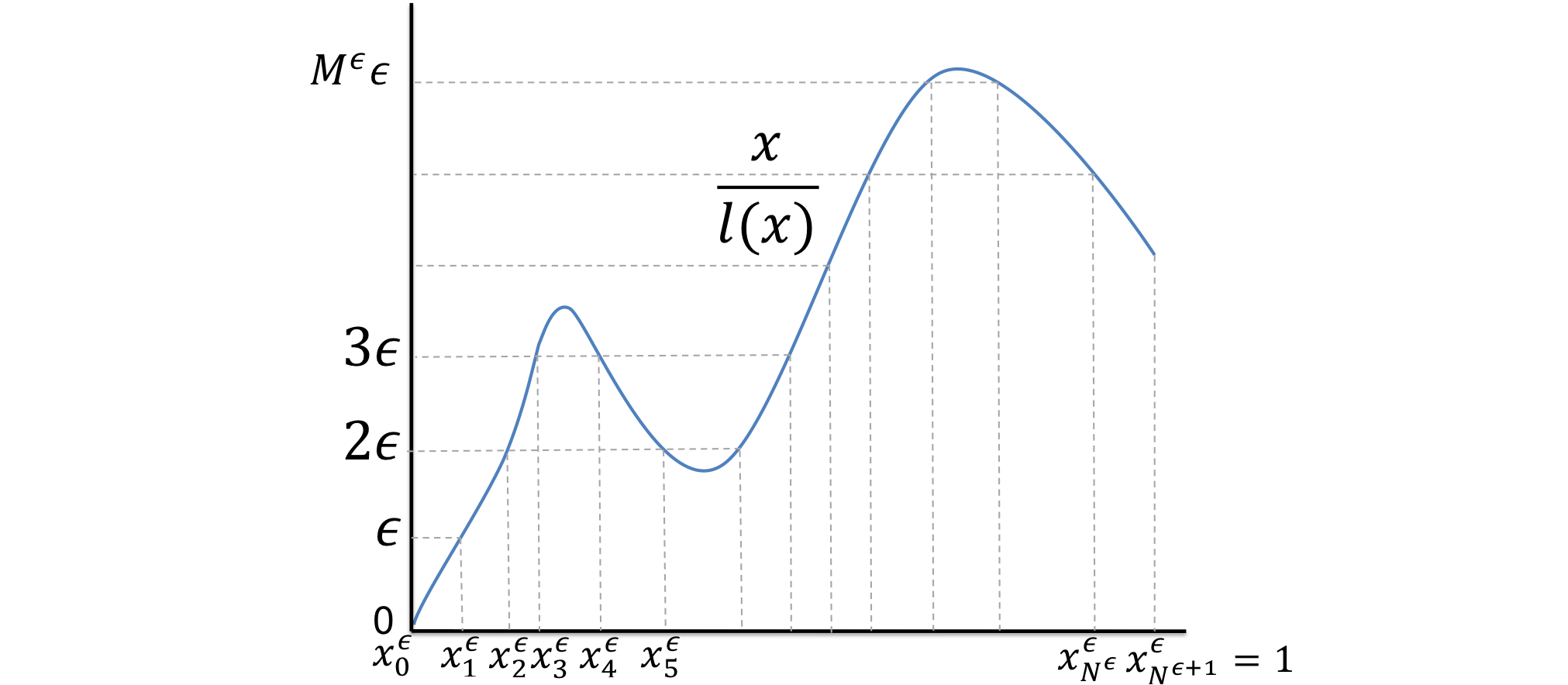
For every ϵ>0\epsilon>0 fixed, we define MϵM^{\epsilon} the largest integer such that Mϵ​ϵ≤maxx∈[0,1]⁡{xl⁡(x)}\displaystyle M^{\epsilon}\epsilon\leq\max_{x\in[0,1]}\Big\{\frac{x}{l(x)}\Big\} and consider the points x∈(0,1)x\in(0,1) such that xl⁡(x)=k​ϵ\frac{x}{l(x)}=k\epsilon, for all k=1,2,…,Mϵk=1,2,\ldots,M^{\epsilon} (see Figure 2). Hence, the l⁡(x)l(x)-partition is defined by {xiϵ}\{x_{i}^{\epsilon}\}, i=0,1,…,Nϵ+1i=0,1,\ldots,N^{\epsilon}+1 such that

  • ∙\bullet

    x0ϵ=0x^{\epsilon}_{0}=0 and xNϵ+1ϵ=1.x_{N^{\epsilon}+1}^{\epsilon}=1.

  • ∙\bullet

    Given xiϵx_{i}^{\epsilon} a point of the partition, i≠Nϵ+1i\neq N^{\epsilon}+1, there exists k∈{0,…,Mϵ}k\in\{0,\dots,M^{\epsilon}\} such that xiϵl⁡(xiϵ)=k​ϵ\frac{x_{i}^{\epsilon}}{l(x_{i}^{\epsilon})}=k\epsilon.

  • ∙\bullet

    Two consecutive points of the partition satisfies
    |xi+1l⁡(xi+1)−xil⁡(xi)|=ϵ, or |xi+1l⁡(xi+1)−xil⁡(xi)|=0\Big|\frac{x_{i+1}}{l(x_{i+1})}-\frac{x_{i}}{l(x_{i})}\Big|=\epsilon,\hbox{ or }\quad\Big|\frac{x_{i+1}}{l(x_{i+1})}-\frac{x_{i}}{l(x_{i})}\Big|=0
Refer to caption
Figure 5: The l⁡(x)l(x)-partition {xkϵ}\{x_{k}^{\epsilon}\}

The l⁡(x)l(x)-partition is correctly defined and it is an admissible partition by assumption (H). This hypothesis guarantees that inverse image of every y∈ℝy\in\mathbb{R} by the function xl⁡(x)\frac{x}{l(x)} is at most a finite set and, as a consequence, the l⁡(x)l(x)-partition has a finite number of points. Moreover, notice that the distance between two consecutive points is not constant but somehow reproduces the locally periodic structure of the thin domain and satisfies that for every x∈(0,1)∖Ax\in(0,1)\setminus A there exist ϵ1>0\epsilon_{1}>0 and a constant CC such that 0≤x−[x]ϵ<C​ϵ, for ​0<ϵ<ϵ1.0\leq x-[x]_{\epsilon}<C\epsilon,\hbox{ for }0<\epsilon<\epsilon_{1}.

Remark 4.2.

To “justify ” the choice of the l⁡(x)l(x)-partition, consider the particular case where the function which defines the oscillatory boundary of the thin domain is given by

G⁡(x,y)=2+cos⁡(2​π​yl⁡(x))G(x,y)=2+\cos\Big(\frac{2\pi y}{l(x)}\Big)

with l⁡(⋅)l(\cdot) verifying the assumption (H). If we look at the points which are at the top part of the oscillatory boundary, that is, G⁡(x,x/ϵ)=3G(x,x/\epsilon)=3, or equivalently,

cos⁡(2​π​xϵ​l​(x))=1,\cos\Big(\frac{2\pi x}{\epsilon l(x)}\Big)=1,

we obtain a sequence of points which verify

2​π​xϵ​l​(x)=2πk,k=0,1,2…\frac{2\pi x}{\epsilon l(x)}=2\pi k,\;k=0,1,2\dots

Observe that these points coincide with the points of the l⁡(x)l(x)-partition. It turns out that these points also work when the amplitude of the oscillations also varies in space since they continue to reproduce in a good way the locally oscillatory behavior of the oscillations.

Remark 4.3.

Observe that hypothesis (H) is a natural assumption to define the l⁡(x)−l(x)-partition. In addition, it allows us to deal with a large kind of period functions. For example, we may consider the case where the function h⁡(x)=xl⁡(x)h(x)=\frac{x}{l(x)} has a finite number of critical points which generates some strange oscillations in the thin domain, (see Figure 2 ).

Moreover, the behavior of the oscillatory boundary is more pathological if we consider for instance a period l⁡(⋅)l(\cdot) such that h⁡(x)h(x) has a countably infinite set of critical points, (see Figure 3).

We start showing the following key property of the partition {xkϵ}\{x_{k}^{\epsilon}\} chosen in this Section.

Proposition 4.4.

If {xkϵ}\{x_{k}^{\epsilon}\} is the l⁡(x)l(x)-partition and with the notation above, we have the following

G⁡([x]ϵ+Γ[x]ϵ​y1,1ϵ​([x]ϵ+Γ[x]ϵ​y1))−G⁡(x,y1)⟶ϵ→00​ a.e ​(x,y1)∈W0.G\big([x]_{\epsilon}+\Gamma_{[x]_{\epsilon}}y_{1},\frac{1}{\epsilon}([x]_{\epsilon}+\Gamma_{[x]_{\epsilon}}y_{1})\big)-G(x,y_{1})\stackrel{{\scriptstyle\epsilon\to 0}}{{\longrightarrow}}0\;\hbox{ a.e }(x,y_{1})\in W_{0}. (4.1)
Proof.

In order to show (4.1), we observe that since G⁡(x,⋅)G(x,\cdot) is l⁡(x)l(x)-periodic and all the points constructed in Definition 4.1 satisfy [x]ϵϵ​l​([x]ϵ)=kϵ∈ℕ\frac{[x]_{\epsilon}}{\epsilon l([x]_{\epsilon})}=k^{\epsilon}\in\mathbb{N} we have

G⁡([x]ϵ+Γ[x]ϵ​y1,1ϵ​([x]ϵ+Γ[x]ϵ​y1))=G⁡([x]ϵ+Γ[x]ϵ​y1,1ϵ​([x]ϵ−l⁡([x]ϵ+Γ[x]ϵ​y1)​[x]ϵl⁡([x]ϵ)+Γ[x]ϵ​y1)).G\Big([x]_{\epsilon}+\Gamma_{[x]_{\epsilon}}y_{1},\frac{1}{\epsilon}\big([x]_{\epsilon}+\Gamma_{[x]_{\epsilon}}y_{1}\big)\Big)=G\Big([x]_{\epsilon}+\Gamma_{[x]_{\epsilon}}y_{1},\frac{1}{\epsilon}\big([x]_{\epsilon}-l\Big([x]_{\epsilon}+\Gamma_{[x]_{\epsilon}}y_{1}\Big)\frac{[x]_{\epsilon}}{l([x]_{\epsilon})}+\Gamma_{[x]_{\epsilon}}y_{1}\big)\Big).

Then, using the regularity properties of G⁡(⋅,⋅)G(\cdot,\cdot) and l⁡(⋅)l(\cdot), see (H), we only have to prove the following convergences for almost every x∈(0,1)x\in(0,1) and y1∈(0,l⁡(x))y_{1}\in(0,l(x)):

[x]ϵ⟶ϵ→0x​a.e ​x∈(0,1).[x]_{\epsilon}\stackrel{{\scriptstyle\epsilon\to 0}}{{\longrightarrow}}x\;\hbox{a.e }x\in(0,1). (4.2)
[x]ϵ+Γ[x]ϵ​y1⟶ϵ→0x,a.e ​(x,y1)∈W0.[x]_{\epsilon}+\Gamma_{[x]_{\epsilon}}y_{1}\stackrel{{\scriptstyle\epsilon\to 0}}{{\longrightarrow}}x,\;\hbox{a.e }(x,y_{1})\in W_{0}. (4.3)
1ϵ​([x]ϵ−l⁡([x]ϵ+Γ[x]ϵ​y1)​[x]ϵl⁡([x]ϵ)+Γ[x]ϵ​y1)⟶ϵ→0y1,a.e ​(x,y1)∈W0.\frac{1}{\epsilon}\Big([x]_{\epsilon}-l\Big([x]_{\epsilon}+\Gamma_{[x]_{\epsilon}}y_{1}\Big)\frac{[x]_{\epsilon}}{l([x]_{\epsilon})}+\Gamma_{[x]_{\epsilon}}y_{1}\Big)\stackrel{{\scriptstyle\epsilon\to 0}}{{\longrightarrow}}y_{1},\;\hbox{a.e }(x,y_{1})\in W_{0}. (4.4)

Since the hypothesis (H) guarantees that the set A has null measure it is enough to prove the convegences of the Proposition for all x∈(0,1)∖Ax\in(0,1)\setminus A.

Let xx be a point in (0,1)∖A(0,1)\setminus A, from the definition of the l⁡(x)−l(x)-partition we know that there exist ϵ1>0\epsilon_{1}>0 and a constant CC such that x∈(xkϵ,xk+1ϵ)x\in(x_{k}^{\epsilon},x_{k+1}^{\epsilon}) and 0<xk+1ϵ−xkϵ<C​ϵ,0<x_{k+1}^{\epsilon}-x_{k}^{\epsilon}<C\epsilon, for some k∈{0,1,2,…,Nϵ+1}k\in\{0,1,2,\dots,N^{\epsilon}+1\} and ∀ 0<ϵ<ϵ1.\forall\,0<\epsilon<\epsilon_{1}. Therefore, the convergences (4.2) and (4.3) are immediate from the definition of [x]ϵ[x]_{\epsilon} and Γ[x]ϵ\Gamma_{[x]_{\epsilon}}.

In order to prove (4.4) we assume that x∈(0,1)∖Ax\in(0,1)\setminus A. From the definition of the l⁡(x)−l(x)-partition we know that for ϵ\epsilon small enough there exists pϵ∈{0,1,…,Mϵ}p^{\epsilon}\in\{0,1,\dots,M^{\epsilon}\} such that [x]ϵ=xkϵ=ϵ​pϵ​l​(xkϵ)[x]_{\epsilon}=x^{\epsilon}_{k}=\epsilon p^{\epsilon}l(x^{\epsilon}_{k}) and xk+1ϵ=ϵ⁡(pϵ+1)​l​(xk+1ϵ)x^{\epsilon}_{k+1}=\epsilon(p^{\epsilon}+1)l(x^{\epsilon}_{k+1}), the function xl⁡(x)\frac{x}{l(x)} increases in the small interval (xkϵ,xk+1ϵ)(x^{\epsilon}_{k},x^{\epsilon}_{k+1}), or xk+1ϵ=ϵ⁡(pϵ−1)​l​(xk+1ϵ)x^{\epsilon}_{k+1}=\epsilon(p^{\epsilon}-1)l(x^{\epsilon}_{k+1}) in case xl⁡(x)\frac{x}{l(x)} decreases. We suppose that xk+1ϵ=ϵ⁡(pϵ+1)​l​(xk+1ϵ)x^{\epsilon}_{k+1}=\epsilon(p^{\epsilon}+1)l(x^{\epsilon}_{k+1}), the proof is similar in the other case.

We study the limit of the following two terms:

(a). Limit of 1ϵ​Γ[x]ϵ​y1\frac{1}{\epsilon}\Gamma_{[x]_{\epsilon}}y_{1}.

Since xk+1ϵ=ϵ⁡(pϵ+1)​l​(xk+1ϵ)x^{\epsilon}_{k+1}=\epsilon(p^{\epsilon}+1)l(x^{\epsilon}_{k+1}) and xkϵ=ϵ​pϵ​l​(xkϵ)x^{\epsilon}_{k}=\epsilon p^{\epsilon}l(x^{\epsilon}_{k}) we have

1ϵ​Γ[x]ϵ​y1=xk+1ϵ−xkϵϵ​l​(xkϵ)​y1=pϵ​y1l⁡(xkϵ)​(l⁡(xk+1ϵ)−l⁡(xkϵ))+y1l⁡(xkϵ)​l​(xk+1ϵ)\displaystyle\frac{1}{\epsilon}\Gamma_{[x]_{\epsilon}}y_{1}=\frac{x^{\epsilon}_{k+1}-x^{\epsilon}_{k}}{\epsilon l(x^{\epsilon}_{k})}y_{1}=p^{\epsilon}\frac{y_{1}}{l(x^{\epsilon}_{k})}\big(l(x^{\epsilon}_{k+1})-l(x^{\epsilon}_{k})\big)+\frac{y_{1}}{l(x^{\epsilon}_{k})}l(x^{\epsilon}_{k+1})
=\displaystyle= xkϵϵ​l​(xkϵ)2​y1​(l⁡(xk+1ϵ)−l⁡(xkϵ))+y1l⁡(xkϵ)​l​(xk+1ϵ)\displaystyle\frac{x^{\epsilon}_{k}}{\epsilon l(x^{\epsilon}_{k})^{2}}y_{1}\big(l(x^{\epsilon}_{k+1})-l(x^{\epsilon}_{k})\big)+\frac{y_{1}}{l(x^{\epsilon}_{k})}l(x^{\epsilon}_{k+1})
=\displaystyle= xkϵl⁡(xkϵ)​y1​l⁡(xk+1ϵ)−l⁡(xkϵ)xk+1ϵ−xkϵ​xk+1ϵ−xkϵϵ​l​(xkϵ)+y1l⁡(xkϵ)​l​(xk+1ϵ)\displaystyle\frac{x^{\epsilon}_{k}}{l(x^{\epsilon}_{k})}y_{1}\frac{l(x^{\epsilon}_{k+1})-l(x^{\epsilon}_{k})}{x^{\epsilon}_{k+1}-x^{\epsilon}_{k}}\frac{x^{\epsilon}_{k+1}-x^{\epsilon}_{k}}{\epsilon l(x^{\epsilon}_{k})}+\frac{y_{1}}{l(x^{\epsilon}_{k})}l(x^{\epsilon}_{k+1})
=\displaystyle= xkϵl⁡(xkϵ)​l⁡(xk+1ϵ)−l⁡(xkϵ)xk+1ϵ−xkϵ​1ϵ​Γ[x]ϵ​y1+y1l⁡(xkϵ)​l​(xk+1ϵ).\displaystyle\frac{x^{\epsilon}_{k}}{l(x^{\epsilon}_{k})}\frac{l(x^{\epsilon}_{k+1})-l(x^{\epsilon}_{k})}{x^{\epsilon}_{k+1}-x^{\epsilon}_{k}}\frac{1}{\epsilon}\Gamma_{[x]_{\epsilon}}y_{1}+\frac{y_{1}}{l(x^{\epsilon}_{k})}l(x^{\epsilon}_{k+1}).

Consequently we obtain

(1−xkϵl⁡(xkϵ)​l⁡(xk+1ϵ)−l⁡(xkϵ)xk+1ϵ−xkϵ)​1ϵ​Γ[x]ϵ​y1=y1l⁡(xkϵ)​l​(xk+1ϵ).\Big(1-\frac{x^{\epsilon}_{k}}{l(x^{\epsilon}_{k})}\frac{l(x^{\epsilon}_{k+1})-l(x^{\epsilon}_{k})}{x^{\epsilon}_{k+1}-x^{\epsilon}_{k}}\Big)\frac{1}{\epsilon}\Gamma_{[x]_{\epsilon}}y_{1}=\frac{y_{1}}{l(x^{\epsilon}_{k})}l(x^{\epsilon}_{k+1}).

Moreover, we can prove that

1−xkϵl⁡(xkϵ)​l⁡(xk+1ϵ)−l⁡(xkϵ)xk+1ϵ−xkϵ≠0for ϵ sufficiently small.1-\frac{x^{\epsilon}_{k}}{l(x^{\epsilon}_{k})}\frac{l(x^{\epsilon}_{k+1})-l(x^{\epsilon}_{k})}{x^{\epsilon}_{k+1}-x^{\epsilon}_{k}}\neq 0\quad\text{for $\epsilon$ sufficiently small}.

If we suppose that this is not true and we pass to the limit then we have , at least for a subsequence, that

l′​(x)=l⁡(x)x.l^{\prime}(x)=\frac{l(x)}{x}.

This contradicts the fact that x∉Ax\not\in A.

Hence we can write

1ϵ​Γ[x]ϵ​y1=(1−xkϵl⁡(xkϵ)​l⁡(xk+1ϵ)−l⁡(xkϵ)xk+1ϵ−xkϵ)−1​y1l⁡(xkϵ)​l​(xk+1ϵ).\frac{1}{\epsilon}\Gamma_{[x]_{\epsilon}}y_{1}=\Big(1-\frac{x^{\epsilon}_{k}}{l(x^{\epsilon}_{k})}\frac{l(x^{\epsilon}_{k+1})-l(x^{\epsilon}_{k})}{x^{\epsilon}_{k+1}-x^{\epsilon}_{k}}\Big)^{-1}\frac{y_{1}}{l(x^{\epsilon}_{k})}l(x^{\epsilon}_{k+1}). (4.5)

Taking into account the above equality (4.5), the hypothesis (H) and x∉Ax\not\in A we get the limit:

1ϵ​Γ[x]ϵ​y1⟶ϵ→0(1−xl⁡(x)​l′​(x))−1​y1.\frac{1}{\epsilon}\Gamma_{[x]_{\epsilon}}y_{1}\stackrel{{\scriptstyle\epsilon\to 0}}{{\longrightarrow}}\Big(1-\frac{x}{l(x)}l^{\prime}(x)\Big)^{-1}y_{1}. (4.6)

(b). Limit of 1ϵ​([x]ϵ−l⁡([x]ϵ+Γ[x]ϵ​y1)​[x]ϵl⁡([x]ϵ))\frac{1}{\epsilon}\Big([x]_{\epsilon}-l\big([x]_{\epsilon}+\Gamma_{[x]_{\epsilon}}y_{1}\big)\frac{[x]_{\epsilon}}{l([x]_{\epsilon})}\Big).

1ϵ​([x]ϵ−l⁡([x]ϵ+Γ[x]ϵ​y1)​[x]ϵl⁡([x]ϵ))=−xkϵl⁡(xkϵ)​l⁡(xkϵ+Γxkϵ​y1)−l⁡(xkϵ)Γxkϵ​y1​Γxkϵ​y1ϵ\displaystyle\frac{1}{\epsilon}\Big([x]_{\epsilon}-l([x]_{\epsilon}+\Gamma_{[x]_{\epsilon}}y_{1})\frac{[x]_{\epsilon}}{l([x]_{\epsilon})}\Big)=-\frac{x^{\epsilon}_{k}}{l(x^{\epsilon}_{k})}\frac{l(x^{\epsilon}_{k}+\Gamma_{x^{\epsilon}_{k}}y_{1})-l(x^{\epsilon}_{k})}{\Gamma_{x^{\epsilon}_{k}}y_{1}}\frac{\Gamma_{x^{\epsilon}_{k}}y_{1}}{\epsilon}

Now it is possible to pass to the limit in the right-hand side by using the convergence (4.6). Hence, we have that

1ϵ​([x]ϵ−l⁡([x]ϵ+Γ[x]ϵ​y1)​[x]ϵl⁡([x]ϵ))⟶ϵ→0−xl⁡(x)​l′​(x)​(1−xl⁡(x)​l′​(x))−1​y1.\frac{1}{\epsilon}\Big([x]_{\epsilon}-l([x]_{\epsilon}+\Gamma_{[x]_{\epsilon}}y_{1})\frac{[x]_{\epsilon}}{l([x]_{\epsilon})}\Big)\stackrel{{\scriptstyle\epsilon\to 0}}{{\longrightarrow}}-\frac{x}{l(x)}l^{\prime}(x)\Big(1-\frac{x}{l(x)}l^{\prime}(x)\Big)^{-1}y_{1}. (4.7)

Therefore, from (4.6) and (4.7), we obtain the converge (4.4)

1ϵ​([x]ϵ−l⁡([x]ϵ+Γ[x]ϵ​y1)​[x]ϵl⁡([x]ϵ)+Γ[x]ϵ​y1)⟶ϵ→0−xl⁡(x)​l′​(x)​(1−xl⁡(x)​l′​(x))−1​y1+(1−xl⁡(x)​l′​(x))−1​y1=y1.\frac{1}{\epsilon}\big([x]_{\epsilon}-l([x]_{\epsilon}+\Gamma_{[x]_{\epsilon}}y_{1})\frac{[x]_{\epsilon}}{l([x]_{\epsilon})}+\Gamma_{[x]_{\epsilon}}y_{1}\big)\stackrel{{\scriptstyle\epsilon\to 0}}{{\longrightarrow}}-\frac{x}{l(x)}l^{\prime}(x)\Big(1-\frac{x}{l(x)}l^{\prime}(x)\Big)^{-1}y_{1}+\Big(1-\frac{x}{l(x)}l^{\prime}(x)\Big)^{-1}y_{1}=y_{1}.

This concludes the proof of the proposition. ∎

We show now that the domains WϵW^{\epsilon}, see (3.1), converge to the domain WW in the sense that the characteristic functions converge strongly in LpL^{p}, 1≤p<∞1\leq p<\infty. Let us denote by χ\chi the characteristic function of WW and by χϵ\chi^{\epsilon} is the characteristic function of RϵR^{\epsilon}. Therefore, Tϵ​(χϵ)T_{\epsilon}(\chi^{\epsilon}) is the characteristic function of WϵW^{\epsilon}. The fact that WϵW^{\epsilon} “ approaches ” WW is expressed in the following result.

Proposition 4.5.

With the notations above and if 𝒯ϵ\mathcal{T}_{\epsilon} is the unfolding operator associated to the l⁡(x)l(x)-partition {xkϵ}\{x_{k}^{\epsilon}\}, we have

𝒯ϵ​(χϵ)⟶χs−Lp​((0,1)×Y∗), for ​1≤p<∞.\mathcal{T_{\epsilon}}(\chi^{\epsilon})\longrightarrow\chi\quad\hbox{s}-L^{p}\big((0,1)\times Y^{*}\big),\hbox{ for }1\leq p<\infty.
Proof.

Since Tϵ​(χϵ)T_{\epsilon}(\chi^{\epsilon}) and χ\chi are uniformly bounded functions (they are actually bounded by the constant 1), it is enough to prove the convergence for p=1p=1. Considering the set represented by each characteristic function we can write:

‖𝒯ϵ​(χϵ)−χ‖L1​((0,1)×Y∗)=\displaystyle\|\mathcal{T_{\epsilon}}(\chi^{\epsilon})-\chi\|_{L^{1}\big((0,1)\times Y^{*}\big)}=
=∫01∫Y∗|χϵ([x]ϵ+Γ[x]ϵy1,ϵy2)χ(0,l⁡([x]ϵ))(y1)−χ(x,y1,y2)|dy1dy2dx\displaystyle=\int_{0}^{1}\int_{Y*}|\chi^{\epsilon}\Big([x]_{\epsilon}+\Gamma_{[x]_{\epsilon}}y_{1},\epsilon y_{2}\Big)\chi_{(0,l([x]_{\epsilon}))}(y_{1})-\chi(x,y_{1},y_{2})|dy_{1}dy_{2}dx
=∫01∫0l⁡([x]ϵ)∫0G⁡([x]ϵ+Γ[x]ϵ​y1,1ϵ​([x]ϵ+Γ[x]ϵ​y1))|1−χ⁡(x,y1,y2)|​d​y2​d​y1​𝑑x\displaystyle=\int_{0}^{1}\int_{0}^{l([x]_{\epsilon})}\int_{0}^{G\Big([x]_{\epsilon}+\Gamma_{[x]_{\epsilon}}y_{1},\frac{1}{\epsilon}\big([x]_{\epsilon}+\Gamma_{[x]_{\epsilon}}y_{1}\big)\Big)}|1-\chi(x,y_{1},y_{2})|dy_{2}dy_{1}dx
+∫01∫0l⁡([x]ϵ)∫G⁡([x]ϵ+Γ[x]ϵ​y1,1ϵ​([x]ϵ+Γ[x]ϵ​y1))G1|χ(x,y1,y2)|dy2dy1dx\displaystyle+\int_{0}^{1}\int_{0}^{l([x]_{\epsilon})}\int_{G\Big([x]_{\epsilon}+\Gamma_{[x]_{\epsilon}}y_{1},\frac{1}{\epsilon}\big([x]_{\epsilon}+\Gamma_{[x]_{\epsilon}}y_{1}\big)\Big)}^{G_{1}}|\chi(x,y_{1},y_{2})|dy_{2}dy_{1}dx
+∫01∫l⁡([x]ϵ)l1∫0G1|χ(x,y1,y2)|dy2dy1dx.\displaystyle+\int_{0}^{1}\int_{l([x]_{\epsilon})}^{l_{1}}\int_{0}^{G_{1}}|\chi(x,y_{1},y_{2})|\;dy_{2}dy_{1}dx.

With the convergence

l⁡([x]ϵ)−l⁡(x)⟶ϵ→00, a.e ​x∈(0,1),l([x]_{\epsilon})-l(x)\stackrel{{\scriptstyle\epsilon\to 0}}{{\longrightarrow}}0,\hbox{ a.e }x\in(0,1), (4.8)

which follows easily from the convergence (4.2) and the continuity of the function l⁡(⋅)l(\cdot), together with (4.1) and with the aid of the Lebesgue’s Dominated Convergence Theorem, we easily prove that ‖𝒯ϵ​(χϵ)−χ‖L1​((0,1)×Y∗)→0.\|\mathcal{T_{\epsilon}}(\chi^{\epsilon})-\chi\|_{L^{1}\big((0,1)\times Y^{*}\big)}\to 0.

∎

Remark 4.6.

The proposition above is basic to get the homogenized limit problem. By using this proposition we will be able to pass to the limit although our unfolded functions are not defined on a fixed domain. Then, it justifies to introduce the set WW which is the expected limit domain.

Remark 4.7.

Note that the choice of the points of the l⁡(x)l(x)-partition is a key point to obtain the convergence of the domains. Somehow, the fact that the partition suitably reflects the geometry of the oscillating domain is very critical to obtain the convergence result. For example, let’s see that things may go wrong if we do not choose wisely the admissible partition, even in the purely periodic case. If we assume that the oscillatory boundary of the thin domain is given by a function g:ℝ→ℝg:\mathbb{R}\to\mathbb{R} LL-periodic and we consider the partition

x0ϵ=0<x1ϵ=ϵ​L1<x2ϵ=2​ϵ​L1<⋯<xNϵϵ=Nϵ​L1<xNϵ+1ϵ=1,x_{0}^{\epsilon}=0<x_{1}^{\epsilon}=\epsilon L_{1}<x_{2}^{\epsilon}=2\epsilon L_{1}<\cdots<x_{N^{\epsilon}}^{\epsilon}=N^{\epsilon}L_{1}<x_{N^{\epsilon}+1}^{\epsilon}=1,

where L1L_{1} is rationally independent of LL. Notice that this partition is an admissible one, but in this case, Proposition 4.4 does not hold, precisely because L1L_{1} and LL are rationally independent.

Proposition 4.8.

Let φ∈Lp​(0,1)\varphi\in L^{p}(0,1), 1≤p<∞1\leq p<\infty. Then if 𝒯ϵ\mathcal{T}_{\epsilon} is the unfolding operator associated to the l⁡(x)l(x)-partition, we have

𝒯ϵ​(φ)⟶φ​χs−Lp​((0,1)×Y∗).\mathcal{T_{\epsilon}(\varphi)}\longrightarrow\varphi\chi\quad\hbox{s}-L^{p}\big((0,1)\times Y^{*}\big).
Proof.

The result is obvious for any φ∈𝒟⁡(0,1)\varphi\in\mathcal{D}(0,1). By density, if φ∈Lp​(0,1)\varphi\in L^{p}(0,1), let φk∈𝒟⁡(0,1)\varphi_{k}\in\mathcal{D}(0,1) such that φk→φ\varphi_{k}\rightarrow\varphi in Lp​(0,1)L^{p}(0,1). Then, we have

‖𝒯ϵ​(φ)−φ​χ‖Lp​((0,1)×Y∗)⩽‖𝒯ϵ​(φ)−𝒯ϵ​(φk)‖Lp​((0,1)×Y∗)\displaystyle\|\mathcal{T_{\epsilon}(\varphi)}-\varphi\chi\|_{L^{p}\big((0,1)\times Y^{*}\big)}\leqslant\|\mathcal{T_{\epsilon}(\varphi)}-\mathcal{T_{\epsilon}}(\varphi_{k})\|_{L^{p}\big((0,1)\times Y^{*}\big)}
+‖𝒯ϵ​(φk)−φk​χ‖Lp​((0,1)×Y∗)+‖φk​χ−φ​χ‖Lp​((0,1)×Y∗)\displaystyle+\|\mathcal{T_{\epsilon}}(\varphi_{k})-\varphi_{k}\chi\|_{L^{p}\big((0,1)\times Y^{*}\big)}+\|\varphi_{k}\chi-\varphi\chi\|_{L^{p}\big((0,1)\times Y^{*}\big)}

from which the result is straightforward. ∎

As we mentioned at the end of Section 2, see Remark 3.4, we need to establish a link between test functions in RϵR^{\epsilon} and test functions in WW. Now, we study the convergence of these functions.

Proposition 4.9.

Let ψ=ψ⁡(x,y1,y2)\psi=\psi(x,y_{1},y_{2}) be a C#∞​(W)C^{\infty}_{\#}(W) function. We define the following function ψϵ∈C∞​(Rϵ¯)\psi^{\epsilon}\in C^{\infty}(\overline{R^{\epsilon}}) by

ψϵ​(x,y)=ψ⁡(x,xϵ,yϵ)∀(x,y)∈Rϵ.\psi^{\epsilon}(x,y)=\psi\big(x,\frac{x}{\epsilon},\frac{y}{\epsilon})\quad\forall(x,y)\in R^{\epsilon}.

Then if 𝒯ϵ\mathcal{T}_{\epsilon} is the unfolding operator associated to the l⁡(x)l(x)-partition

𝒯ϵ​(ψϵ)⟶ψ​χs−Lp​((0,1)×Y∗),∀1≤p<∞.\mathcal{T_{\epsilon}(\psi^{\epsilon})}\longrightarrow\psi\chi\quad\hbox{s}-L^{p}\big((0,1)\times Y^{*}\big),\forall 1\leq p<\infty.
Proof.

We have already shown that ψϵ\psi^{\epsilon} is well defined, see Proposition 3.3, v). Then, we only have to prove the convergence.

‖𝒯ϵ​(ψϵ)−ψ​χ‖Lp​((0,1)×Y∗)p=\displaystyle\|\mathcal{T_{\epsilon}(\psi^{\epsilon})}-\psi\chi\|^{p}_{L^{p}\big((0,1)\times Y^{*}\big)}=
=∫01∫Y∗|ψϵ([x]ϵ+Γ[x]ϵy1,ϵy2)𝒯ϵ(χϵ)(x,y1,y2)−ψ(x,y1,y2)χ(x,y1,y2)|pdy1dy2dx\displaystyle=\int_{0}^{1}\int_{Y*}\big|\psi^{\epsilon}\Big([x]_{\epsilon}+\Gamma_{[x]_{\epsilon}}y_{1},\epsilon y_{2}\Big)\mathcal{T_{\epsilon}(\chi^{\epsilon})}(x,y_{1},y_{2})-\psi(x,y_{1},y_{2})\chi(x,y_{1},y_{2})\big|^{p}dy_{1}dy_{2}dx
=∫01∫Y∗|ψ([x]ϵ+Γ[x]ϵy1,1ϵ([x]ϵ+Γ[x]ϵy1),y2)𝒯ϵ(χϵ)−ψχ|pdy1dy2dx.\displaystyle=\int_{0}^{1}\int_{Y*}\big|\psi\Big([x]_{\epsilon}+\Gamma_{[x]_{\epsilon}}y_{1},\frac{1}{\epsilon}\big([x]_{\epsilon}+\Gamma_{[x]_{\epsilon}}y_{1}\big),y_{2}\Big)\mathcal{T_{\epsilon}(\chi^{\epsilon})}-\psi\chi\big|^{p}dy_{1}dy_{2}dx.

Since ψ\psi is continuous on WW and taking into account the convergences (4.3) and (4.4) we have

|ψ⁡([x]ϵ+Γ[x]ϵ​y1,1ϵ​([x]ϵ−l⁡([x]ϵ+Γ[x]ϵ​y1)​[x]ϵl⁡([x]ϵ)+Γ[x]ϵ​y1),y2)−ψ⁡(x,y1,y2)|⟶ϵ→00​ a.e on ​W.\big|\psi\Big([x]_{\epsilon}+\Gamma_{[x]_{\epsilon}}y_{1},\frac{1}{\epsilon}\big([x]_{\epsilon}-l\Big([x]_{\epsilon}+\Gamma_{[x]_{\epsilon}}y_{1}\Big)\frac{[x]_{\epsilon}}{l([x]_{\epsilon})}+\Gamma_{[x]_{\epsilon}}y_{1}\big),y_{2}\Big)-\psi(x,y_{1},y_{2})\big|\stackrel{{\scriptstyle\epsilon\to 0}}{{\longrightarrow}}0\;\hbox{ a.e on }W. (4.9)

Hence, due to (4.9), Proposition 4.5 and by applying the Lebesgue’s Dominated Convergence Theorem we obtain the result. ∎

So far we have only considered functions in Lp​(Rϵ)L^{p}(R^{\epsilon}). Now we study the behavior of sequences in W1,p​(Rϵ)W^{1,p}(R^{\epsilon}). We will prove a compactness result which allows us to obtain the limit of the unfolded derivatives. Before that, we need to state and prove a technical Lemma which we will use later on.

Lemma 4.10.

Assume 1≤p<∞1\leq p<\infty. For any function θ⁡(⋅)∈W01,p​(0,1)\theta(\cdot)\in W^{1,p}_{0}(0,1) there exists a function ψ\psi in Lp​((0,1),W#1,p​(Y∗​(x)))L^{p}\Big((0,1);W^{1,p}_{\#}\big(Y^{*}(x)\big)\Big) such that

ψ=ψ⁡(x,y2), in ​W\psi=\psi(x,y_{2}),\hbox{ in }W
ψ⁡(x,y2)=0on∂W∖B1,\psi(x,y_{2})=0\quad\hbox{on}\quad\partial{W}\setminus B_{1},
1l⁡(x)​∫Y∗​(x)ψ⁡(x,y2)​d​y1​d​y2=θ⁡(x)∀x∈(0,1),\frac{1}{l(x)}\int_{Y^{*}(x)}\psi(x,y_{2})dy_{1}dy_{2}=\theta(x)\quad\forall x\in(0,1),
‖ψ‖Lp​(W)⩽C​‖θ‖Lp​(0,1),\|\psi\|_{L^{p}(W)}\leqslant C\|\theta\|_{L^{p}(0,1)},

where B1B_{1} is the following lateral boundary of WW

B1={(x,0,y2):x∈(0,1)​and​ 0<y2<G⁡(x,0)}​⋃{(x,l⁡(x),y2):x∈(0,1)​and​ 0<y2<G⁡(x,0)}.B_{1}=\left\{(x,0,y_{2}):x\in(0,1)\;\hbox{and}\;0<y_{2}<G(x,0)\right\}\bigcup\left\{(x,l(x),y_{2}):x\in(0,1)\;\hbox{and}\;0<y_{2}<G(x,0)\right\}.
Proof.

Let us consider the cell Y0∗=(0,l0)×(0,G0)⊂Y∗​(x),∀x∈(0,1)Y^{*}_{0}=(0,l_{0})\times(0,G_{0})\subset Y^{*}(x),\;\forall x\in(0,1). We define the following auxiliary problem:

{−∂2v∂y22=1 in ​Y0∗∂v∂y1=0 in ​Y0∗v=0on ​A1∪A2\left\{\begin{gathered}-\frac{\partial^{2}v}{{\partial y_{2}}^{2}}=1\quad\textrm{ in }Y^{*}_{0}\\ \frac{\partial v}{\partial y_{1}}=0\quad\textrm{ in }Y^{*}_{0}\\ v=0\quad\textrm{on }A_{1}\cup A_{2}\end{gathered}\right.

where A1A_{1} is the upper boundary and A2A_{2} is the lower boundary of Y0∗.Y^{*}_{0}.

This problem admits an unique, nonzero solution that we can obtain explicitly:

v⁡(y2)=−y222+G02​y2∀y2∈(0,G0).v(y_{2})=-\frac{y_{2}^{2}}{2}+\frac{G_{0}}{2}y_{2}\quad\forall y_{2}\in(0,G_{0}).

Then we define the function ψ\psi by:

ψ⁡(x,y1,y2)=l0∫Y0∗(∂v∂y2)2​d​y1​d​y2​v~​(y2)​θ​(x)∀(x,y1,y2)∈W.\psi(x,y_{1},y_{2})=\frac{l_{0}}{\int_{Y^{*}_{0}}\Big(\frac{\partial v}{\partial y_{2}}\Big)^{2}dy_{1}dy_{2}}\;\widetilde{v}(y_{2})\theta(x)\quad\forall(x,y_{1},y_{2})\in W.

Since ∫Y0∗(∂v∂y2)2​d​y1​d​y2=∫Y0∗v​d​y1​d​y2\int_{Y^{*}_{0}}\Big(\frac{\partial v}{\partial y_{2}}\Big)^{2}dy_{1}dy_{2}=\int_{Y^{*}_{0}}v\,dy_{1}dy_{2}, it is easy to see that ψ\psi satisfies all the properties of the Lemma. ∎

We are now in position to state the main result of this section.

Theorem 4.11.

Let φϵ∈W1,p​(Rϵ)\varphi^{\epsilon}\in W^{1,p}(R^{\epsilon}) for 1≤p<∞1\leq p<\infty, with |||φϵ|||W1,p​(Rϵ)=ϵ−1/p∥φϵ∥W1,p​(Rϵ)|||\varphi^{\epsilon}|||_{W^{1,p}(R^{\epsilon})}=\epsilon^{-1/p}\|\varphi^{\epsilon}\|_{W^{1,p}(R^{\epsilon})} uniformly bounded. Then, if 𝒯ϵ\mathcal{T}_{\epsilon} is the unfolding operator associated to the l⁡(x)l(x)-partition

  1. i)

    There exists a function φ\varphi in W1,p​(0,1)W^{1,p}(0,1) such that, up to subsequences:

    𝒯ϵ​(φϵ)⇀φ​χw−Lp​((0,1)×Y∗).\mathcal{T_{\epsilon}(\varphi^{\epsilon})}\rightharpoonup\varphi\chi\quad\hbox{w}-L^{p}\big((0,1)\times Y^{*}\big).
  2. ii)

    There exists a function φ1\varphi_{1} in Lp​((0,1),W#1,p​(Y∗​(x)))L^{p}\Big((0,1);W^{1,p}_{\#}(Y^{*}(x))\Big) such that, up to subsequences:

    𝒯ϵ​(∂φϵ∂x)⇀ξ0​(x,y1,y2)={∂φ∂x​(x)+l⁡(x)​∂φ1∂y1​(x,y1,y2)for(x,y1,y2)∈W0for(x,y1,y2)∈(0,1)×Y∗∖W.\displaystyle\mathcal{T_{\epsilon}}\Big(\frac{\partial\varphi^{\epsilon}}{\partial x}\Big)\rightharpoonup\xi_{0}(x,y_{1},y_{2})=\left\{\begin{array}[]{ll}\frac{\partial\varphi}{\partial x}(x)+l(x)\frac{\partial\varphi_{1}}{\partial y_{1}}(x,y_{1},y_{2})\quad\hbox{for}\quad(x,y_{1},y_{2})\in W\\ 0\quad\quad\hbox{for}\quad(x,y_{1},y_{2})\in(0,1)\times Y^{*}\setminus W.\end{array}\right.
    𝒯ϵ​(∂φϵ∂y)⇀ξ1​(x,y1,y2)={l⁡(x)​∂φ1∂y2​(x,y1,y2)for(x,y1,y2)∈W0for(x,y1,y2)∈(0,1)×Y∗∖W.\displaystyle\mathcal{T_{\epsilon}}\Big(\frac{\partial\varphi^{\epsilon}}{\partial y}\Big)\rightharpoonup\xi_{1}(x,y_{1},y_{2})=\left\{\begin{array}[]{ll}l(x)\frac{\partial\varphi_{1}}{\partial y_{2}}(x,y_{1},y_{2})\quad\hbox{for}\quad(x,y_{1},y_{2})\in W\\ 0\quad\quad\hbox{for}\quad(x,y_{1},y_{2})\in(0,1)\times Y^{*}\setminus W.\end{array}\right.
Proof.

i) Since the norm ‖|φϵ|‖Lp​(Rϵ)|||\varphi^{\epsilon}|||_{L^{p}(R^{\epsilon})} is uniformly bounded in ϵ\epsilon, using Proposition 3.3, iv), we deduce that ‖𝒯ϵ​(φ)‖Lp​((0,1)×Y∗)\|\mathcal{T_{\epsilon}(\varphi)}\|_{L^{p}\big((0,1)\times Y^{*}\big)} is also uniformly bounded and, therefore, we can extract a subsequence of 𝒯ϵ​(φϵ)\mathcal{T_{\epsilon}(\varphi^{\epsilon})}, still denoted by 𝒯ϵ​(φϵ)\mathcal{T_{\epsilon}(\varphi^{\epsilon})} such that

𝒯ϵ​(φϵ)⇀φ^w−Lp​((0,1)×Y∗).\mathcal{T_{\epsilon}(\varphi^{\epsilon})}\rightharpoonup\hat{\varphi}\quad\hbox{w}-L^{p}\big((0,1)\times Y^{*}\big).

To check that φ^\hat{\varphi} is zero outside WW is obvious from Definition 3.2 and Proposition 4.5.

Now we prove that φ^\hat{\varphi} does not depend on (y1,y2)(y_{1},y_{2}) in WW. For this, let Ψ=(ψ1,ψ2)\Psi=(\psi_{1},\psi_{2}) be a function in [𝒟⁡(W)]2[\mathcal{D}(W)]^{2}. We also denote by Ψ\Psi the extension by zero and notice that it belongs to [𝒟⁡((0,1)×Y∗)]2.[\mathcal{D}\big((0,1)\times Y^{*}\big)]^{2}. Using Proposition 3.3, v), we can define Ψϵ≡(ψ,ϵ1ψ)ϵ2∈[𝒟(Rϵ)]2\Psi^{\epsilon}\equiv(\psi{{}_{1}}^{\epsilon},\psi{{}_{2}}^{\epsilon})\in[\mathcal{D}(R^{\epsilon})]^{2}, where

ψ(x,y)ϵi=ψi(x,xϵ,yϵ)∀(x,y)∈Rϵ,i=1,2.\psi{{}_{i}}^{\epsilon}(x,y)=\psi_{i}(x,\frac{x}{\epsilon},\frac{y}{\epsilon})\;\;\forall\,(x,y)\in R^{\epsilon},\quad i=1,2.

In addition, set

θ(x,y)ϵ1=∂ψ1∂x(x,xϵ,yϵ),θ(x,y)ϵ2=∂ψ1∂y1(x,xϵ,yϵ) and θ(x,y)ϵ3=∂ψ2∂y2(x,xϵ,yϵ).\theta{{}_{1}}^{\epsilon}(x,y)=\frac{\partial\psi_{1}}{\partial x}(x,\frac{x}{\epsilon},\frac{y}{\epsilon}),\;\theta{{}_{2}}^{\epsilon}(x,y)=\frac{\partial\psi_{1}}{\partial y_{1}}(x,\frac{x}{\epsilon},\frac{y}{\epsilon})\hbox{ and }\theta{{}_{3}}^{\epsilon}(x,y)=\frac{\partial\psi_{2}}{\partial y_{2}}(x,\frac{x}{\epsilon},\frac{y}{\epsilon}).

Integrating by parts, we have

∫Rϵ∇φϵ(x,y)⋅Ψ(x,xϵ,yϵ)dxdy=−∫Rϵφϵ(x,y)(θ(x,y)ϵ1+1ϵθ(x,y)ϵ2+1ϵθ(x,y)ϵ3)dxdy.\int_{R^{\epsilon}}\nabla\varphi^{\epsilon}(x,y)\cdot\Psi(x,\frac{x}{\epsilon},\frac{y}{\epsilon})dxdy=-\int_{R^{\epsilon}}\varphi^{\epsilon}(x,y)\Big(\theta{{}_{1}}^{\epsilon}(x,y)+\frac{1}{\epsilon}\theta{{}_{2}}^{\epsilon}(x,y)+\frac{1}{\epsilon}\theta{{}_{3}}^{\epsilon}(x,y)\Big)dxdy.

Then, by the criterion for integrals, Proposition 3.3, we obtain

∫(0,1)×Y∗ϵl⁡([x]ϵ)​{𝒯ϵ​(∂φϵ∂x)​𝒯ϵ​(ψ1ϵ)+𝒯ϵ​(∂φϵ∂y)​𝒯ϵ​(ψ2ϵ)}​𝑑x​d​y1​d​y2\displaystyle\int_{(0,1)\times Y^{*}}\frac{\epsilon}{l([x]_{\epsilon})}\left\{\mathcal{T_{\epsilon}}\Big(\frac{\partial\varphi^{\epsilon}}{\partial x}\Big)\mathcal{T_{\epsilon}}(\psi^{\epsilon}_{1})+\mathcal{T_{\epsilon}}\Big(\frac{\partial\varphi^{\epsilon}}{\partial y}\Big)\mathcal{T_{\epsilon}}(\psi^{\epsilon}_{2})\right\}dxdy_{1}dy_{2}
=\displaystyle= −∫(0,1)×Y∗1l⁡([x]ϵ){ϵ𝒯ϵ(φϵ)𝒯ϵ(θ)ϵ1+𝒯ϵ(φϵ)𝒯ϵ(θ)ϵ2+𝒯ϵ(φϵ)𝒯ϵ(θ)ϵ3}dxdy1dy2.\displaystyle-\int_{(0,1)\times Y^{*}}\frac{1}{l([x]_{\epsilon})}\left\{\epsilon\mathcal{T_{\epsilon}(\varphi^{\epsilon})}\mathcal{T_{\epsilon}}(\theta{{}_{1}}^{\epsilon})+\mathcal{T_{\epsilon}(\varphi^{\epsilon})}\mathcal{T_{\epsilon}}(\theta{{}_{2}}^{\epsilon})+\mathcal{T_{\epsilon}(\varphi^{\epsilon})}\mathcal{T_{\epsilon}}(\theta{{}_{3}}^{\epsilon})\right\}dxdy_{1}dy_{2}.

Passing to the limit in both terms with the help of Proposition 4.5 and Proposition 4.9 we get

0=−∫W1l⁡(x)φ^(x,y1,y2)divy1​y2Ψ(x,y1,y2)dxdy1dy2∀Ψ∈[𝒟(W)]2.0=-\int_{W}\frac{1}{l(x)}\hat{\varphi}(x,y_{1},y_{2})\hbox{div}_{y_{1}y_{2}}\Psi(x,y_{1},y_{2})dxdy_{1}dy_{2}\quad\forall\Psi\in[\mathcal{D}(W)]^{2}.

This implies that φ^\hat{\varphi} does not depend on (y1,y2)(y_{1},y_{2}) in WW. Then we can conclude that there exists a function φ∈Lp​(0,1)\varphi\in L^{p}(0,1) such that:

φ^​(x,y1,y2)=φ⁡(x)​χ​(x,y1,y2)∀(x,y1,y2)∈(0,1)×Y∗.\hat{\varphi}(x,y_{1},y_{2})=\varphi(x)\chi(x,y_{1},y_{2})\quad\forall(x,y_{1},y_{2})\in(0,1)\times Y^{*}.

We see now that φ∈W1,p​(0,1)\varphi\in W^{1,p}(0,1). For this, for any function θ⁡(x)∈𝒟⁡(0,1)\theta(x)\in\mathcal{D}(0,1) let ψ\psi be the function in W1,q​(W)W^{1,q}(W), 1p+1q=1\frac{1}{p}+\frac{1}{q}=1, given by Lemma 4.10, that is

∂ψ∂y1=0 in ​W\frac{\partial\psi}{\partial y_{1}}=0\quad\textrm{ in }W
ψ⁡(x,y2)=0on∂W−B1,\psi(x,y_{2})=0\quad\hbox{on}\quad\partial{W}-B_{1},
1l⁡(x)​∫Y∗​(x)ψ⁡(x,y2)​d​y1​d​y2=θ⁡(x)∀x∈(0,1),\frac{1}{l(x)}\int_{Y^{*}(x)}\psi(x,y_{2})dy_{1}dy_{2}=\theta(x)\quad\forall x\in(0,1),
‖ψ‖Lq​(W)⩽C​‖θ‖Lq​(0,1),\|\psi\|_{L^{q}(W)}\leqslant C\|\theta\|_{L^{q}(0,1)},

where B​1B1 is the lateral boundary of W defined in Lemma 4.10. Note that the extension by zero of ψ\psi in the direction y2y_{2} belongs to the space W1,q​((0,1)×Y∗)W^{1,q}((0,1)\times Y^{*}\big). We define the sequence {ψϵ}\{\psi^{\epsilon}\} by

ψϵ​(x,y)=ψ⁡(x,yϵ)∀(x,y)∈Rϵ.\psi^{\epsilon}(x,y)=\psi(x,\frac{y}{\epsilon})\quad\forall(x,y)\in R^{\epsilon}.

Integrating by parts, we obtain

∫Rϵ∂φϵ∂x(x,y)ψϵ(x,y)dxdy=−∫Rϵφϵ(x,y)∂ψϵ∂x(x,y)dxdy.\int_{R^{\epsilon}}\frac{\partial\varphi^{\epsilon}}{\partial x}(x,y)\psi^{\epsilon}(x,y)dxdy=-\int_{R^{\epsilon}}\varphi^{\epsilon}(x,y)\frac{\partial\psi^{\epsilon}}{\partial x}(x,y)dxdy.

Then, by the unfolding criterion for integrals, we have

∫(0,1)×Y∗1l⁡([x]ϵ)𝒯ϵ(∂φϵ∂x)𝒯ϵ(ψϵ)dxdy1dy2=−∫(0,1)×Y∗1l⁡([x]ϵ)𝒯ϵ(φϵ)𝒯ϵ(∂ψϵ∂x)dxdy1dy2.\int_{(0,1)\times Y^{*}}\frac{1}{l([x]_{\epsilon})}\mathcal{T_{\epsilon}}\Big(\frac{\partial\varphi^{\epsilon}}{\partial x}\Big)\mathcal{T_{\epsilon}(\psi^{\epsilon})}dxdy_{1}dy_{2}=-\int_{(0,1)\times Y^{*}}\frac{1}{l([x]_{\epsilon})}\mathcal{T_{\epsilon}(\varphi^{\epsilon})}\mathcal{T_{\epsilon}}\Big(\frac{\partial\psi^{\epsilon}}{\partial x}\Big)dxdy_{1}dy_{2}. (4.12)

We can pass to the limit in (4.12) using Proposition 4.5 , Proposition 4.9 and assuming that 𝒯ϵ​(∂φϵ∂x)⇀ξ0​(x,y1,y2)\mathcal{T_{\epsilon}}\Big(\frac{\partial\varphi^{\epsilon}}{\partial x}\Big)\rightharpoonup\xi_{0}(x,y_{1},y_{2}) w-Lp​((0,1)×Y∗)L^{p}\big((0,1)\times Y^{*}\big), it will be seen in the second part of Theorem. Thus, we get

∫W1l⁡(x)ξ0(x,y1,y2)ψ(x,y2)dxdy1dy2=−∫W1l⁡(x)φ(x)∂ψ∂x(x,y2)dxdy1dy2.\int_{W}\frac{1}{l(x)}\xi_{0}(x,y_{1},y_{2})\psi(x,y_{2})dxdy_{1}dy_{2}=-\int_{W}\frac{1}{l(x)}\varphi(x)\frac{\partial\psi}{\partial x}(x,y_{2})dxdy_{1}dy_{2}. (4.13)

By using Lemma 4.10 above, the right-hand side of (4.13) becomes ∫(0,1)φ⁡(x)​∂θ∂x​(x)​𝑑x,\int_{(0,1)}\varphi(x)\frac{\partial\theta}{\partial x}(x)dx, while the left-hand side is a linear continuous form in θ⁡(x)∈𝒟⁡(0,1).\theta(x)\in\mathcal{D}(0,1). This implies that φ∈W1,p​(0,1).\varphi\in W^{1,p}(0,1).

ii) Since |||φϵ|||W1,p​(Rϵ)=ϵ−1/p∥φϵ∥W1,p​(Rϵ)|||\varphi^{\epsilon}|||_{W^{1,p}(R^{\epsilon})}=\epsilon^{-1/p}\|\varphi^{\epsilon}\|_{W^{1,p}(R^{\epsilon})} is uniformly bounded, using property iv) in Proposition 3.3 we can extract two subsequences of 𝒯ϵ​(∂φϵ∂x)\mathcal{T_{\epsilon}}\Big(\frac{\partial\varphi^{\epsilon}}{\partial x}\Big) and 𝒯ϵ​(∂φϵ∂y)\mathcal{T_{\epsilon}}\Big(\frac{\partial\varphi^{\epsilon}}{\partial y}\Big), still denoted by 𝒯ϵ​(∂φϵ∂x)\mathcal{T_{\epsilon}}\Big(\frac{\partial\varphi^{\epsilon}}{\partial x}\Big) and 𝒯ϵ​(∂φϵ∂y)\mathcal{T_{\epsilon}}\Big(\frac{\partial\varphi^{\epsilon}}{\partial y}\Big) such that

𝒯ϵ​(∂φϵ∂x)⇀ξ0​(x,y1,y2)w−Lp​((0,1)×Y∗),\mathcal{T_{\epsilon}}\Big(\frac{\partial\varphi^{\epsilon}}{\partial x}\Big)\rightharpoonup\xi_{0}(x,y_{1},y_{2})\quad\hbox{w}-L^{p}\big((0,1)\times Y^{*}\big),
𝒯ϵ​(∂φϵ∂y)⇀ξ1​(x,y1,y2)w−Lp​((0,1)×Y∗),\mathcal{T_{\epsilon}}\Big(\frac{\partial\varphi^{\epsilon}}{\partial y}\Big)\rightharpoonup\xi_{1}(x,y_{1},y_{2})\quad\hbox{w}-L^{p}\big((0,1)\times Y^{*}\big),

for certain ξ0\xi_{0} and ξ1\xi_{1} in Lp​((0,1)×Y∗).L^{p}\big((0,1)\times Y^{*}\big).

First note that ξ0=ξ1=0\xi_{0}=\xi_{1}=0 in (0,1)×Y∗\W(0,1)\times Y^{*}\backslash W follows from the definition of unfolding operator and Proposition 4.5.

In order to find the precise form of ξ0\xi_{0} and ξ1\xi_{1} in WW we argue as follows.

Let Ψ≡(ψ1,ψ2)∈[C#∞​(W)]2\Psi\equiv(\psi_{1},\psi_{2})\in\big[C^{\infty}_{\#}(W)\big]^{2} be a function satisfying

divy1​y2​Ψ=0\hbox{div}_{y_{1}y_{2}}\Psi=0
Ψ⁡(x,y1,y2)⋅n(y1,y2)​(x)=0​on​∂i​n​fY∗​(x)∪∂s​u​pY∗​(x),\Psi(x,y_{1},y_{2})\cdot n_{(y_{1},y_{2})}(x)=0\;\hbox{on}\;\partial_{inf}Y^{*}(x)\cup\partial_{sup}Y^{*}(x),
ψ1​(0,⋅,⋅)=ψ1​(1,⋅,⋅)=0,\psi_{1}(0,\cdot,\cdot)=\psi_{1}(1,\cdot,\cdot)=0,

where n(y1,y2)​(x)n_{(y_{1},y_{2})}(x) is the outward normal to ∂Y∗​(x)\partial Y^{*}(x) for every x∈(0,1)x\in(0,1).

From Proposition 4.9 we can define Ψϵ≡(ψ,ϵ1ψ)ϵ2∈[W1,p(Rϵ)]2\Psi^{\epsilon}\equiv(\psi{{}_{1}}^{\epsilon},\psi{{}_{2}}^{\epsilon})\in[W^{1,p}(R^{\epsilon})]^{2}, where

ψ(x,y)ϵi=ψi(x,xϵ,yϵ)∀(x,y)∈Rϵ,i=1,2.\psi{{}_{i}}^{\epsilon}(x,y)=\psi_{i}(x,\frac{x}{\epsilon},\frac{y}{\epsilon})\;\;\forall\,(x,y)\in R^{\epsilon},\quad i=1,2.

Then, integrating by parts, we have

∫Rϵ[∇φϵ​(x,y)−∇φ​(x)]⋅Ψϵ​(x,y)​𝑑x​𝑑y−∫∂s​u​pRϵνϵ⋅Ψϵ​(φϵ−φ)​𝑑S=\displaystyle\int_{R^{\epsilon}}\Big[\nabla\varphi^{\epsilon}(x,y)-\nabla\varphi(x)\Big]\cdot\Psi^{\epsilon}(x,y)\;dxdy-\int_{\partial_{sup}R^{\epsilon}}\nu^{\epsilon}\cdot\Psi^{\epsilon}(\varphi^{\epsilon}-\varphi)\,dS=
=−∫Rϵ[φϵ(x,y)−φ(x)]div(x,y)Ψϵ(x,y)dxdy\displaystyle=-\int_{R^{\epsilon}}\Big[\varphi^{\epsilon}(x,y)-\varphi(x)\Big]\hbox{div}_{(x,y)}\Psi^{\epsilon}(x,y)\;dxdy
=−∫Rϵ{[φϵ(x,y)−φ(x)]∂ψ1∂x(x,xϵ,yϵ)+1ϵ[φϵ(x,y)−φ(x)]div(y1,y2)Ψ(x,xϵ,yϵ)}dxdy\displaystyle=-\int_{R^{\epsilon}}\left\{\Big[\varphi^{\epsilon}(x,y)-\varphi(x)\Big]\frac{\partial\psi_{1}}{\partial x}(x,\frac{x}{\epsilon},\frac{y}{\epsilon})+\frac{1}{\epsilon}\Big[\varphi^{\epsilon}(x,y)-\varphi(x)\Big]\hbox{div}_{(y_{1},y_{2})}\Psi(x,\frac{x}{\epsilon},\frac{y}{\epsilon})\right\}dxdy
=−∫Rϵ[φϵ(x,y)−φ(x)]∂ψ1∂x(x,xϵ,yϵ)dxdy.\displaystyle=-\int_{R^{\epsilon}}\Big[\varphi^{\epsilon}(x,y)-\varphi(x)\Big]\frac{\partial\psi_{1}}{\partial x}(x,\frac{x}{\epsilon},\frac{y}{\epsilon})dxdy. (4.14)

Applying the unfolding criterion for integrals we can write (4.14) as:

∫(0,1)×Y∗1l⁡([x]ϵ)​{[𝒯ϵ​(∂φϵ∂x)−𝒯ϵ​(∂φ∂x)]​𝒯ϵ​(ψ1)+𝒯ϵ​(∂φϵ∂y)​𝒯ϵ​(ψ2)}​𝑑x​d​y1​d​y2\displaystyle\int_{(0,1)\times Y^{*}}\frac{1}{l([x]_{\epsilon})}\left\{\Big[\mathcal{T_{\epsilon}}\Big(\frac{\partial\varphi^{\epsilon}}{\partial x}\Big)-\mathcal{T_{\epsilon}}\Big(\frac{\partial\varphi}{\partial x}\Big)\Big]\mathcal{T_{\epsilon}}(\psi_{1})+\mathcal{T_{\epsilon}}\Big(\frac{\partial\varphi^{\epsilon}}{\partial y}\Big)\mathcal{T_{\epsilon}}(\psi_{2})\right\}dxdy_{1}dy_{2}
=−∫(0,1)×Y∗1l⁡([x]ϵ)[𝒯ϵ(φϵ)−𝒯ϵ(φ)]𝒯ϵ(∂ψ1∂x)dxdy1dy2+1ϵ∫∂s​u​pRϵνϵ⋅Ψϵ(φϵ−φ)dS.\displaystyle=-\int_{(0,1)\times Y^{*}}\frac{1}{l([x]_{\epsilon})}\Big[\mathcal{T_{\epsilon}(\varphi^{\epsilon})}-\mathcal{T_{\epsilon}(\varphi)}\Big]\mathcal{T_{\epsilon}}\Big(\frac{\partial\psi_{1}}{\partial x}\Big)dxdy_{1}dy_{2}+\frac{1}{\epsilon}\int_{\partial_{sup}R^{\epsilon}}\nu^{\epsilon}\cdot\Psi^{\epsilon}(\varphi^{\epsilon}-\varphi)\,dS. (4.15)

Now, we prove that the boundary term vanishes as ϵ\epsilon tends to zero. The unit normal to ∂s​u​pRϵ\partial_{sup}R^{\epsilon} is given by

νϵ=(−ϵ​Gx−Gy(ϵ​Gx+Gy)2+1,1(ϵ​Gx+Gy)2+1),\nu^{\epsilon}=\Big(\frac{-\epsilon G_{x}-G_{y}}{\sqrt{(\epsilon G_{x}+G_{y})^{2}+1}},\frac{1}{\sqrt{(\epsilon G_{x}+G_{y})^{2}+1}}\Big),

where Gx=∂G∂x\displaystyle{G_{x}=\frac{\partial G}{\partial x}} and Gy=∂G∂yG_{y}=\displaystyle{\frac{\partial G}{\partial y}}.

Then, taking into account Ψ⁡(x,y1,y2)⋅n(y1,y2)​(x)=0​on​∂s​u​pY∗​(x)\Psi(x,y_{1},y_{2})\cdot n_{(y_{1},y_{2})}(x)=0\;\hbox{on}\;\partial_{sup}Y^{*}(x) we have

∫∂s​u​pRϵνϵ⋅Ψϵ(φϵ−φ)dS=−ϵ∫∂s​u​pRϵGx(ϵ​Gx+Gy)2+1ψ1ϵ(φϵ−φ)dS\int_{\partial_{sup}R^{\epsilon}}\nu^{\epsilon}\cdot\Psi^{\epsilon}(\varphi^{\epsilon}-\varphi)\,dS=-\epsilon\int_{\partial_{sup}R^{\epsilon}}\frac{G_{x}}{\sqrt{(\epsilon G_{x}+G_{y})^{2}+1}}\psi_{1}^{\epsilon}(\varphi^{\epsilon}-\varphi)\,dS

Therefore, since ‖|Gx(ϵ​Gx+Gy)2+1​ψ1ϵ​(φϵ−φ)|‖W1,1​(Rϵ)\displaystyle{\Big|\Big|\Big|\frac{G_{x}}{\sqrt{(\epsilon G_{x}+G_{y})^{2}+1}}\psi_{1}^{\epsilon}(\varphi^{\epsilon}-\varphi)\Big|\Big|\Big|_{W^{1,1}(R^{\epsilon})}} is uniformly bounded we can conclude

limϵ→01ϵ​∫∂s​u​pRϵνϵ​Ψϵ​(φϵ−φ)​𝑑S=0.\lim_{\epsilon\to 0}\frac{1}{\epsilon}\int_{\partial_{sup}R^{\epsilon}}\nu^{\epsilon}\Psi^{\epsilon}(\varphi^{\epsilon}-\varphi)\,dS=0. (4.16)

Passing to the limit in (4.15) with the help of Proposition 4.5, Proposition 4.9, the convergence in i) and (4.16) we get

∫W1l⁡(x)​{[ξ0​(x,y1,y2)−∂φ∂x​(x)]​ψ1​(x,y1,y2)+ξ1​(x,y1,y2)​ψ2​(x,y1,y2)}​𝑑x​d​y1​d​y2=0.\int_{W}\frac{1}{l(x)}\left\{\Big[\xi_{0}(x,y_{1},y_{2})-\frac{\partial\varphi}{\partial x}(x)\Big]\psi_{1}(x,y_{1},y_{2})+\xi_{1}(x,y_{1},y_{2})\psi_{2}(x,y_{1},y_{2})\right\}dxdy_{1}dy_{2}=0.

Hence, we obtain

∫W(1l⁡(x)​[ξ0​(x,y1,y2)−∂φ∂x​(x)],1l⁡(x)​ξ1​(x,y1,y2))⋅(ψ1,ψ2)​(x,y1,y2)​𝑑x​d​y1​d​y2=0.\int_{W}\Big(\frac{1}{l(x)}\Big[\xi_{0}(x,y_{1},y_{2})-\frac{\partial\varphi}{\partial x}(x)\Big],\frac{1}{l(x)}\xi_{1}(x,y_{1},y_{2})\Big)\cdot\big(\psi_{1},\psi_{2}\big)(x,y_{1},y_{2})dxdy_{1}dy_{2}=0. (4.17)

The Helmholtz decomposition, see [23], yields that the orthogonal of divergence-free functions is exactly the gradients. Then, we can conclude that there exists a function φ1∈Lp​((0,1),W#1,p​(Y∗​(x)))\varphi_{1}\in L^{p}\Big((0,1);W^{1,p}_{\#}\big(Y^{*}(x)\big)\Big) such that

1l⁡(x)​(ξ0​(x,y1,y2)−∂φ∂x​(x))=∂φ1∂y1​(x,y1,y2)∀(x,y1,y2)∈W,\frac{1}{l(x)}\Big(\xi_{0}(x,y_{1},y_{2})-\frac{\partial\varphi}{\partial x}(x)\Big)=\frac{\partial\varphi_{1}}{\partial y_{1}}(x,y_{1},y_{2})\quad\forall(x,y_{1},y_{2})\in W,
1l⁡(x)​ξ1​(x,y1,y2)=∂φ1∂y2​(x,y1,y2)∀(x,y1,y2)∈W,\frac{1}{l(x)}\xi_{1}(x,y_{1},y_{2})=\frac{\partial\varphi_{1}}{\partial y_{2}}(x,y_{1},y_{2})\quad\forall(x,y_{1},y_{2})\in W,

which ends the proof of the Theorem.

∎

Remark 4.12.

As we wrote in the introduction, this Theorem is the main tool to obtain the homogenized limit problem. On one hand, it shows that the limit φ\varphi lies in W1,p​(0,1),W^{1,p}(0,1), which was not clear at all in view of the a priori estimates because 𝒯ϵ​(φϵ)\mathcal{T_{\epsilon}(\varphi^{\epsilon})} is defined on a varying set. On the other hand, it allows us to relate the limit of the unfolded derivatives 𝒯ϵ​(∂φϵ∂x)\mathcal{T_{\epsilon}}\Big(\frac{\partial\varphi^{\epsilon}}{\partial x}\Big) and 𝒯ϵ​(∂φϵ∂y)\mathcal{T_{\epsilon}}\Big(\frac{\partial\varphi^{\epsilon}}{\partial y}\Big) with the weak derivative of φ\varphi. Note that the variable period plays a decisive role in the limit and, as we will see in the next section, it enters into the limit equation.

Remark 4.13.

The proof provided for Theorem 4.11 uses similar techniques as in [2]. It is also possible to obtain the same result by adapting the scale-splitting operators, 𝒬ϵ\mathcal{Q_{\epsilon}} and ℛϵ\mathcal{R_{\epsilon}}, introduced in [18] to the new situation presented in this paper. However, the calculations using these operators are a little bit more involved.

5 Homogenization of the Neumman problem

In this section we return to the problem (1.1) presented in the Introduction and we show how the unfolding operator method adapted to this new situation allows to obtain the homogenized limit problem. We will need the results from the previous Sections and in particular the convergence result from Theorem 4.11. Therefore, throughout this Section we will assume that the unfolding operator 𝒯ϵ\mathcal{T}_{\epsilon} is the one associated to the l⁡(x)l(x)-partition.

We start by recalling the problem:

{−Δ​uϵ+uϵ=fϵ in ​Rϵ∂uϵ∂νϵ=0 on ​∂Rϵ\left\{\begin{gathered}-\Delta u^{\epsilon}+u^{\epsilon}=f^{\epsilon}\quad\textrm{ in }R^{\epsilon}\\ \frac{\partial u^{\epsilon}}{\partial\nu^{\epsilon}}=0\quad\textrm{ on }\partial R^{\epsilon}\end{gathered}\right. (5.1)

with fϵ∈L2​(Rϵ)f^{\epsilon}\in L^{2}(R^{\epsilon}) and where νϵ=(ν1ϵ,ν2ϵ)\nu^{\epsilon}=(\nu^{\epsilon}_{1},\nu^{\epsilon}_{2}) is the unit outward normal to ∂Rϵ\partial R^{\epsilon} and ∂∂νϵ\frac{\partial}{\partial\nu^{\epsilon}} is the outside normal derivative. The domain RϵR^{\epsilon} is a two dimensional thin domain which is given by

Rϵ={(x,y)∈ℝ2|x∈(0,1), 0<y<ϵG(x,x/ϵ)}R^{\epsilon}=\{(x,y)\in\mathbb{R}^{2}\;|\;x\in(0,1),\,0<y<\epsilon\,G(x,x/\epsilon)\}

where G⁡(⋅,⋅)G(\cdot,\cdot) is a function satisfying the assumptions established in Section 2. From Lax-Milgran Theorem, we have that problem (5.1) has a unique solution for each ϵ>0\epsilon>0. We are interested here in analyzing the behavior of the solutions as ϵ→0\epsilon\to 0.

The variational formulation of (5.1) is

{Find​uϵ∈H1​(Rϵ)​such that∫Rϵ{∇uϵ⋅∇φ+uϵ​φ}​dx​dy=∫Rϵfϵ​φ​dx​dy,∀φ∈H1​(Rϵ).\displaystyle\left\{\begin{array}[]{lll}\text{Find}\;u^{\epsilon}\in H^{1}(R^{\epsilon})\;\text{such that}\\ \\ \displaystyle\int_{R^{\epsilon}}\Big\{\nabla u^{\epsilon}\cdot\nabla\varphi+u^{\epsilon}\varphi\Big\}dxdy=\int_{R^{\epsilon}}f^{\epsilon}\varphi dxdy,\\ \\ \forall\varphi\in H^{1}(R^{\epsilon}).\end{array}\right.

Now we are in condition to state and prove the homogenization result.

Theorem 5.1.

Let uϵu^{\epsilon} be the solution of problem (5.1). Assume that fϵ∈L2​(Rϵ)f^{\epsilon}\in L^{2}(R^{\epsilon}) satisfies ‖|fϵ|‖L2​(Rϵ)≤C|||f^{\epsilon}|||_{L^{2}(R^{\epsilon})}\leq C with C independent of the parameter ϵ\epsilon and, therefore, there exists f^∈L2​(W)\hat{f}\in L^{2}(W) such that, via subsequences, 𝒯ϵ​(fϵ)⇀f^​χweakly in ​L2​((0,1)×Y∗)\displaystyle{\mathcal{T_{\epsilon}}(f^{\epsilon})\rightharpoonup\hat{f}\chi\quad\hbox{weakly in }\;L^{2}\big((0,1)\times Y^{*}\big)}. Then, there exist u∈H1​(0,1)u\in H^{1}(0,1) and u1∈L2​((0,1),H#1​(Y∗​(x)))u_{1}\in L^{2}\Big((0,1);H^{1}_{\#}\big(Y^{*}(x)\big)\Big) such that

𝒯ϵ​(uϵ)⇀u^=u​χweakly in ​L2​((0,1)×Y∗),\displaystyle\displaystyle{\mathcal{T_{\epsilon}}(u^{\epsilon})\rightharpoonup\hat{u}=u\chi\quad\hbox{weakly in }\;L^{2}\big((0,1)\times Y^{*}\big),} (5.8)
𝒯ϵ​(∂uϵ∂x)⇀ξ0​(x,y1,y2)=∂u∂x​(x)+l⁡(x)​∂u1∂y1​(x,y1,y2)weakly in ​L2​(W),\displaystyle\displaystyle{\mathcal{T_{\epsilon}}\Big(\frac{\partial u^{\epsilon}}{\partial x}\Big)\rightharpoonup\xi_{0}(x,y_{1},y_{2})=\frac{\partial u}{\partial x}(x)+l(x)\frac{\partial u_{1}}{\partial y_{1}}(x,y_{1},y_{2})\quad\hbox{weakly in }\;L^{2}(W),} (5.9)
𝒯ϵ​(∂uϵ∂y)⇀ξ1​(x,y1,y2)=l⁡(x)​∂u1∂y2​(x,y1,y2)weakly in ​L2​(W),\displaystyle\displaystyle{\mathcal{T_{\epsilon}}\Big(\frac{\partial u^{\epsilon}}{\partial y}\Big)\rightharpoonup\xi_{1}(x,y_{1},y_{2})=l(x)\frac{\partial u_{1}}{\partial y_{2}}(x,y_{1},y_{2})\quad\quad\hbox{weakly in }\;L^{2}(W),} (5.10)

and the pair (u,u1)(u,u_{1}) is the unique solution of the problem

{∀ϕ∈H1​(0,1),∀ψ∈L2​((0,1),H#1​(Y∗​(x)))∫W{(1l⁡(x)​∂u∂x​(x)+∂u1∂y1​(x,y1,y2))​(∂ϕ∂x​(x)+∂ψ∂y1​(x,y1,y2))}​dx​d​y1​d​y2+∫W{∂u1∂y2(x,y1,y2)∂ψ∂y2(x,y1,y2)+u⁡(x)​ϕ​(x)l⁡(x)}dxdy1dy2=∫Wf^​(x,y1,y2)​ϕ​(x)l⁡(x)dxdy1dy2.\left\{\begin{gathered}\forall\phi\in H^{1}(0,1),\forall\psi\in L^{2}\Big((0,1);H^{1}_{\#}\big(Y^{*}(x)\big)\Big)\\ \int_{W}\left\{\Big(\frac{1}{l(x)}\frac{\partial u}{\partial x}(x)+\frac{\partial u_{1}}{\partial y_{1}}(x,y_{1},y_{2})\Big)\Big(\frac{\partial\phi}{\partial x}(x)+\frac{\partial\psi}{\partial y_{1}}(x,y_{1},y_{2})\Big)\right\}dxdy_{1}dy_{2}\\ +\int_{W}\left\{\,\frac{\partial u_{1}}{\partial y_{2}}(x,y_{1},y_{2})\frac{\partial\psi}{\partial y_{2}}(x,y_{1},y_{2})+\frac{u(x)\phi(x)}{l(x)}\right\}dxdy_{1}dy_{2}=\int_{W}\frac{\hat{f}(x,y_{1},y_{2})\phi(x)}{l(x)}dxdy_{1}dy_{2}.\end{gathered}\right. (5.11)

Equivalently, u∈H1​(0,1)u\in H^{1}(0,1) is the unique weak solution of the following Neumann problem, it was obtained through the relation u1​(x,y1,y2)=−X⁡(x)​(y1,y2)​1l⁡(x)​∂u∂x​(x)u_{1}(x,y_{1},y_{2})=-X(x)(y_{1},y_{2})\frac{1}{l(x)}\frac{\partial u}{\partial x}(x),

{−(r⁡(x)​ux)x+|Y∗​(x)|l⁡(x)​u=f0,x∈(0,1)u′​(0)=u′​(1)=0\left\{\begin{gathered}-\big(r(x)u_{x}\big)_{x}+\frac{|Y^{*}(x)|}{l(x)}u=f_{0},\quad x\in(0,1)\\ u^{\prime}(0)=u^{\prime}(1)=0\end{gathered}\right. (5.12)

where

f0=1l⁡(x)​∫Y∗​(x)f^​d​y1​d​y2,\begin{gathered}f_{0}=\frac{1}{l(x)}\int_{Y^{*}(x)}\hat{f}dy_{1}dy_{2},\\ \end{gathered} (5.13)
r⁡(x)=1l⁡(x)​∫Y∗​(x){1−∂X⁡(x)∂y1​(y1,y2)}​d​y1​d​y2\begin{gathered}r(x)=\frac{1}{l(x)}\int_{Y^{*}(x)}\Big\{1-\frac{\partial X(x)}{\partial y_{1}}(y_{1},y_{2})\Big\}dy_{1}dy_{2}\\ \end{gathered} (5.14)

and X⁡(x)X(x) is the unique solution which is l⁡(x)l(x)-periodic in the first variable, of the problem

{−Δ​X​(x)=0​ in ​Y∗​(x)∂X⁡(x)∂N=0​ on ​B2​(x)∂X⁡(x)∂N=N1​(x)​ on ​B1​(x)∫Y∗​(x)X⁡(x)​d​y1​d​y2=0\left\{\begin{gathered}-\Delta X(x)=0\textrm{ in }Y^{*}(x)\\ \frac{\partial X(x)}{\partial N}=0\textrm{ on }B_{2}(x)\\ \frac{\partial X(x)}{\partial N}=N_{1}(x)\textrm{ on }B_{1}(x)\\ \int_{Y^{*}(x)}X(x)\;dy_{1}dy_{2}=0\end{gathered}\right. (5.15)

in the representative cell Y∗​(x)Y^{*}(x) given by

Y∗(x)={(y1,y2)∈ℝ2: 0<y1<l(x),0<y2<G(x,y1)}.Y^{*}(x)=\{(y_{1},y_{2})\in\mathbb{R}^{2}\;:\;0<y_{1}<l(x),\quad 0<y_{2}<G(x,y_{1})\}. (5.16)

B1​(x)B_{1}(x) is the upper boundary and B2​(x)B_{2}(x) is the lower boundary of ∂Y∗​(x)\partial Y^{*}(x) for all x∈Ix\in I.

Remark 5.2.

Observe that the limit equation (5.12) reflects the geometry of the thin domain. As it is reasonable to expect , the family of solutions converge to a function of just one variable which satisfies a elliptic equation in one dimension and the variable period appears explicitly in this equation.

Proof.

We start by establishing a priori estimates of uϵu^{\epsilon}. In fact, taking φ=uϵ\varphi=u^{\epsilon} in the variational formulation (5), we obtain

‖∂uϵ∂x‖L2​(Rϵ)2+‖∂uϵ∂y‖L2​(Rϵ)2+‖uϵ‖L2​(Rϵ)2≤‖fϵ‖L2​(Rϵ)​‖uϵ‖L2​(Rϵ).\begin{gathered}\Big\|\frac{\partial u^{\epsilon}}{\partial x}\Big\|_{L^{2}(R^{\epsilon})}^{2}+\Big\|\frac{\partial u^{\epsilon}}{\partial y}\Big\|_{L^{2}(R^{\epsilon})}^{2}+\|u^{\epsilon}\|_{L^{2}(R^{\epsilon})}^{2}\leq\|f^{\epsilon}\|_{L^{2}(R^{\epsilon})}\|u^{\epsilon}\|_{L^{2}(R^{\epsilon})}.\end{gathered} (5.17)

Consequently,

‖|∂uϵ∂x|‖L2​(Rϵ)2+|‖∂uϵ∂y‖|L2​(Rϵ)2+|​‖uϵ‖|L2​(Rϵ)2≤‖|fϵ|‖L2​(Rϵ)|‖uϵ‖|L2​(Rϵ).\begin{gathered}\Big|\Big|\Big|\frac{\partial u^{\epsilon}}{\partial x}\Big|\Big|\Big|_{L^{2}(R^{\epsilon})}^{2}+\Big|\Big|\Big|\frac{\partial u^{\epsilon}}{\partial y}\Big|\Big|\Big|_{L^{2}(R^{\epsilon})}^{2}+|||u^{\epsilon}|||_{L^{2}(R^{\epsilon})}^{2}\leq|||f^{\epsilon}|||_{L^{2}(R^{\epsilon})}|||u^{\epsilon}|||_{L^{2}(R^{\epsilon})}.\end{gathered} (5.18)

Taking into account that there exists C>0C>0, independent of ϵ\epsilon, such that |||fϵ|||L2​(Rϵ)|||⩽C|||f^{\epsilon}|||_{L^{2}(R^{\epsilon})}|||\leqslant C, we obtain

‖|uϵ|‖L2​(Rϵ),‖|∂uϵ∂x|‖L2​(Rϵ)​ and |‖∂uϵ∂y‖|L2​(Rϵ)≤C∀ϵ>0.\begin{gathered}|||u^{\epsilon}|||_{L^{2}(R^{\epsilon})},\Big|\Big|\Big|\frac{\partial u^{\epsilon}}{\partial x}\Big|\Big|\Big|_{L^{2}(R^{\epsilon})}\textrm{ and }\Big|\Big|\Big|\frac{\partial u^{\epsilon}}{\partial y}\Big|\Big|\Big|_{L^{2}(R^{\epsilon})}\leq C\quad\forall\epsilon>0.\end{gathered} (5.19)

Therefore, the compactness Theorem 4.11 implies that there exist u∈H1​(0,1)u\in H^{1}(0,1) and u1∈L2​((0,1),H#1​(Y∗​(x)))u_{1}\in L^{2}\Big((0,1);H^{1}_{\#}\big(Y^{*}(x)\big)\Big) such that

𝒯ϵ​(uϵ)⇀u^=u​χweakly in ​L2​((0,1)×Y∗),𝒯ϵ​(∂uϵ∂x)⇀ξ0​(x,y1,y2)=∂u∂x​(x)+l⁡(x)​∂u1∂y1​(x,y1,y2)weakly in ​L2​(W),𝒯ϵ​(∂uϵ∂y)⇀ξ1​(x,y1,y2)=l⁡(x)​∂u1∂y2​(x,y1,y2)weakly in ​L2​(W).\displaystyle\begin{array}[]{lll}\displaystyle{\mathcal{T_{\epsilon}}(u^{\epsilon})\rightharpoonup\hat{u}=u\chi\quad\hbox{weakly in }\;L^{2}\big((0,1)\times Y^{*}\big),}\\ \\ \displaystyle{\mathcal{T_{\epsilon}}\Big(\frac{\partial u^{\epsilon}}{\partial x}\Big)\rightharpoonup\xi_{0}(x,y_{1},y_{2})=\frac{\partial u}{\partial x}(x)+l(x)\frac{\partial u_{1}}{\partial y_{1}}(x,y_{1},y_{2})\quad\hbox{weakly in }\;L^{2}(W),}\\ \\ \displaystyle{\mathcal{T_{\epsilon}}\Big(\frac{\partial u^{\epsilon}}{\partial y}\Big)\rightharpoonup\xi_{1}(x,y_{1},y_{2})=l(x)\frac{\partial u_{1}}{\partial y_{2}}(x,y_{1},y_{2})\quad\quad\hbox{weakly in }\;L^{2}(W).}\\ \end{array}

We are now in the position of finding the homogenized equations satisfied by uu and u1u_{1}. Let us apply the unfolding operator to the original variational formulation (5). For ϕ∈H1​(0,1)\phi\in H^{1}(0,1), by the unfolding criterion for integrals (3.2), we have

∫(0,1)×Y∗1l⁡([x]ϵ)​{𝒯ϵ​(∂uϵ∂x)​𝒯ϵ​(∂ϕ∂x)+𝒯ϵ​(uϵ)​𝒯ϵ​(ϕ)}​𝑑x​d​y1​d​y2=∫(0,1)×Y∗1l⁡([x]ϵ)​𝒯ϵ​(fϵ)​𝒯ϵ​(ϕ)​𝑑x​d​y1​d​y2.\displaystyle\int_{(0,1)\times Y^{*}}\frac{1}{l([x]_{\epsilon})}\left\{\mathcal{T_{\epsilon}}\Big(\frac{\partial u^{\epsilon}}{\partial x}\Big)\mathcal{T_{\epsilon}}(\frac{\partial\phi}{\partial x})+\mathcal{T_{\epsilon}}(u^{\epsilon})\mathcal{T_{\epsilon}}(\phi)\right\}dxdy_{1}dy_{2}=\int_{(0,1)\times Y^{*}}\frac{1}{l([x]_{\epsilon})}\mathcal{T_{\epsilon}}(f^{\epsilon})\mathcal{T_{\epsilon}(\phi)}dxdy_{1}dy_{2}.

Observe that in this last equality we have taken ϕ∈H1​(0,1)\phi\in H^{1}(0,1) and the term including partial derivative with respect to yy does not appear. By the convergences of (5)(\ref{main convergence}) together with Proposition 4.8 we can pass to the limit in the last equality and we obtain the first equation:

∫W{(1l⁡(x)​∂u∂x​(x)+∂u1∂y1​(x,y1,y2))​∂ϕ∂x​(x)+u⁡(x)​ϕ​(x)l⁡(x)}​𝑑x​d​y1​d​y2=\displaystyle\int_{W}\left\{\Big(\frac{1}{l(x)}\frac{\partial u}{\partial x}(x)+\frac{\partial u_{1}}{\partial y_{1}}(x,y_{1},y_{2})\Big)\frac{\partial\phi}{\partial x}(x)+\frac{u(x)\phi(x)}{l(x)}\right\}dxdy_{1}dy_{2}=
=∫Wf^​(x)​ϕ​(x)l⁡(x)​𝑑x​d​y1​d​y2,∀ϕ∈H1​(0,1).\displaystyle=\int_{W}\frac{\hat{f}(x)\phi(x)}{l(x)}dxdy_{1}dy_{2},\quad\forall\phi\in H^{1}(0,1). (5.26)

We take now as a test function in (5) the function vϵv^{\epsilon} defined by:

vϵ​(x,y)=ϵ​ψ​(x,xϵ,yϵ)∀(x,y)∈Rϵv^{\epsilon}(x,y)=\epsilon\psi(x,\frac{x}{\epsilon},\frac{y}{\epsilon})\quad\forall(x,y)\in R^{\epsilon}

where ψ∈C#∞​(W)\psi\in C^{\infty}_{\#}(W).

It is obvious from the definition that vϵ∈H1​(Rϵ)v^{\epsilon}\in H^{1}(R^{\epsilon}). Furthermore, it satisfies

∂vϵ∂x=ϵ​∂ψ∂x+∂ψ∂y1,\frac{\partial v^{\epsilon}}{\partial x}=\epsilon\frac{\partial\psi}{\partial x}+\frac{\partial\psi}{\partial y_{1}},
∂vϵ∂y=∂ψ∂y2.\frac{\partial v^{\epsilon}}{\partial y}=\frac{\partial\psi}{\partial y_{2}}.

Hence, using the properties of the unfolding operator we can show,

𝒯ϵ​(vϵ)→0s-​L2​((0,1)×Y∗),𝒯ϵ​(∂vϵ∂x)→∂ψ∂y1​χs-​L2​((0,1)×Y∗),𝒯ϵ​(∂vϵ∂y)→∂ψ∂y2​χs-​L2​((0,1)×Y∗).\displaystyle\begin{array}[]{lll}\displaystyle{\mathcal{T_{\epsilon}}(v^{\epsilon})\rightarrow 0\quad\hbox{s-}L^{2}((0,1)\times Y^{*}),}\\ \\ \displaystyle{\mathcal{T_{\epsilon}}\Big(\frac{\partial v^{\epsilon}}{\partial x}\Big)\rightarrow\frac{\partial\psi}{\partial y_{1}}\chi\quad\hbox{s-}L^{2}((0,1)\times Y^{*}),}\\ \\ \displaystyle{\mathcal{T_{\epsilon}}\Big(\frac{\partial v^{\epsilon}}{\partial y}\Big)\rightarrow\frac{\partial\psi}{\partial y_{2}}\chi\quad\hbox{s-}L^{2}((0,1)\times Y^{*}).}\\ \\ \end{array}

Due to the unfolding criterion for integrals, from the variational formulation (5) we obtain

∫(0,1)×Y∗1l⁡([x]ϵ)​{𝒯ϵ​(∂uϵ∂x)​𝒯ϵ​(∂vϵ∂x)+𝒯ϵ​(∂uϵ∂y)​𝒯ϵ​(∂vϵ∂y)+𝒯ϵ​(uϵ)​𝒯ϵ​(vϵ)}​𝑑x​d​y1​d​y2\displaystyle\int_{(0,1)\times Y^{*}}\frac{1}{l([x]_{\epsilon})}\left\{\mathcal{T_{\epsilon}}\Big(\frac{\partial u^{\epsilon}}{\partial x}\Big)\mathcal{T_{\epsilon}}\Big(\frac{\partial v^{\epsilon}}{\partial x}\Big)+\mathcal{T_{\epsilon}}\Big(\frac{\partial u^{\epsilon}}{\partial y}\Big)\mathcal{T_{\epsilon}}\Big(\frac{\partial v^{\epsilon}}{\partial y}\Big)+\mathcal{T_{\epsilon}}(u^{\epsilon})\mathcal{T_{\epsilon}}(v^{\epsilon})\right\}dxdy_{1}dy_{2}
=∫(0,1)×Y∗1l⁡([x]ϵ)​𝒯ϵ​(fϵ)​𝒯ϵ​(vϵ)​𝑑x​d​y1​d​y2.\displaystyle=\int_{(0,1)\times Y^{*}}\frac{1}{l([x]_{\epsilon})}\mathcal{T_{\epsilon}}(f^{\epsilon})\mathcal{T_{\epsilon}}(v^{\epsilon})dxdy_{1}dy_{2}. (5.34)

Now using the three statements in (5) and (5), we pass to the limit in (5.34) and we obtain the second equation:

∫W(1l⁡(x)​∂u∂x​(x)+∂u1∂y1​(x,y1,y2))​∂ψ∂y1​(x,y1,y2)​𝑑x​d​y1​d​y2\displaystyle\int_{W}\Big(\frac{1}{l(x)}\frac{\partial u}{\partial x}(x)+\frac{\partial u_{1}}{\partial y_{1}}(x,y_{1},y_{2})\Big)\frac{\partial\psi}{\partial y_{1}}(x,y_{1},y_{2})\;dxdy_{1}dy_{2}
+∫W∂u1∂y2(x,y1,y2)∂ψ∂y2(x,y1,y2)dxdy1dy2=0,∀ψ∈C#∞(W).\displaystyle+\int_{W}\frac{\partial u_{1}}{\partial y_{2}}(x,y_{1},y_{2})\frac{\partial\psi}{\partial y_{2}}(x,y_{1},y_{2})\;dxdy_{1}dy_{2}=0,\;\forall\psi\in C^{\infty}_{\#}(W). (5.35)

By density, (5.35) holds true for any function ψ∈L2​((0,1),H#1​(Y∗​(x)))\psi\in L^{2}\Big((0,1);H^{1}_{\#}\big(Y^{*}(x)\big)\Big). Therefore, by summing (5.26) and (5.35) we have the homogenized system (5.11).

To end the proof we will see the relation between the homogenized system and the classical homogenized equation (5.12). This is achieved by using the solutions of the problem (5.15). Treating xx as a parameter in (5.35) is easy to check that it is a variational formulation associated to the following cell-problem:

{−Δ​u1​(x)=0​ in ​Y∗​(x)∂u1​(x)∂N=0​ on ​B2​(x)∂u1​(x)∂N=−N1​(x)l⁡(x)​∂u∂x​(x)​ on ​B1​(x)u1​(x,⋅,⋅)​l​(x)−periodic in the variable​y1,\left\{\begin{gathered}-\Delta u_{1}(x)=0\textrm{ in }Y^{*}(x)\\ \frac{\partial u_{1}(x)}{\partial N}=0\textrm{ on }B_{2}(x)\\ \frac{\partial u_{1}(x)}{\partial N}=\frac{-N_{1}(x)}{l(x)}\frac{\partial u}{\partial x}(x)\textrm{ on }B_{1}(x)\\ u_{1}(x,\cdot,\cdot)\;l(x)-\hbox{periodic in the variable}\;y_{1},\\ \end{gathered}\right. (5.36)

where N⁡(x)=(N1​(x),N2​(x))N(x)=(N_{1}(x),N_{2}(x)) is the unit outward normal to ∂Y∗​(x)\partial Y^{*}(x), B1​(x)B_{1}(x) is the upper boundary and B2​(x)B_{2}(x) is the lower boundary of ∂Y∗​(x)\partial Y^{*}(x) for all x∈Ix\in I. Thus, taking into account uu is independent of (y1,y2)(y_{1},y_{2}) one can see inmediatly that:

u1​(x,y1,y2)=−X⁡(x)​(y1,y2)​1l⁡(x)​∂u∂x​(x)​(x,y1,y2)∈W,u_{1}(x,y_{1},y_{2})=-X(x)(y_{1},y_{2})\frac{1}{l(x)}\frac{\partial u}{\partial x}(x)\;(x,y_{1},y_{2})\in W, (5.37)

where X⁡(x)X(x) is the solution of (5.15).
Replacing u1u_{1} by its value, (5.37), in the equation (5.26) we obtain the weak formulation of (5.12).

The uniqueness and existence of weak solution of the problem (5.12) is an inmediate consequence of the Lax-Milgram theorem.

∎

Remark 5.3.

If the non homogeneous term fϵ​(x,y)f^{\epsilon}(x,y) is a fixed function depending only on the first variable, that is, fϵ​(x,y)=f⁡(x)f^{\epsilon}(x,y)=f(x), it is easy to see that f0​(x)=|Y∗​(x)|l⁡(x)​f​(x)f_{0}(x)=\frac{|Y^{*}(x)|}{l(x)}f(x) and therefore, (5.12) can be written as

{−l⁡(x)|Y∗​(x)|​(r⁡(x)​ux)x+u=f,x∈(0,1)u′​(0)=u′​(1)=0\left\{\begin{gathered}-\frac{l(x)}{|Y^{*}(x)|}\big(r(x)u_{x}\big)_{x}+u=f,\quad x\in(0,1)\\ u^{\prime}(0)=u^{\prime}(1)=0\end{gathered}\right.
Remark 5.4.

Notice that in case GϵG_{\epsilon} presents a purely periodic behavior we recover the homogenized limit problem obtained in [4]. On the other hand, in case the amplitude of the oscillation depends on xx but the period is constant, l⁡(x)≡Ll(x)\equiv L, we obtain the same homogenized limit problem as in [5].

6 Corrector result for the Neumann problem

In this section we address the question of correctors for problem (5.1). To do that, we need the averaging operator 𝒰ϵ\mathcal{U}_{\epsilon}, adapted to locally periodic thin domains, see [19] for the definition for a purely periodic case. In principle, this operator could be associated to any “admissible partition” {xkϵ}\{x_{k}^{\epsilon}\} but since we will use it in connection with convergence properties of the solutions and will use the results from previous sections, we will consider it is already associated to the l⁡(x)l(x)-partition, see Definition 4.1. Hence, we define

Definition 6.1.

Let {xkϵ}\{x_{k}^{\epsilon}\} be the l⁡(x)l(x)-partition. Then, if φ∈Lp​((0,1)×Y∗)\varphi\in L^{p}((0,1)\times Y^{*}), p∈[1,∞]p\in[1,\infty], we set

𝒰ϵ​(φ)​(x,y)=1l⁡([x]ϵ)​∫0l⁡([x]ϵ)φ⁡([x]ϵ+Γ[x]ϵ​y1,x−[x]ϵΓ[x]ϵ,yϵ)​d​y1,∀(x,y)∈Rϵ.\mathcal{U_{\epsilon}}(\varphi)(x,y)=\frac{1}{l([x]_{\epsilon})}\int_{0}^{l([x]_{\epsilon})}\varphi\Big([x]_{\epsilon}+\Gamma_{[x]_{\epsilon}}y_{1},\frac{x-[x]_{\epsilon}}{\Gamma_{[x]_{\epsilon}}},\frac{y}{\epsilon}\Big)\;dy_{1},\quad\forall(x,y)\in R^{\epsilon}.
Proposition 6.2.

The main properties of 𝒰ϵ\mathcal{U}_{\epsilon} are the following:

  1. i)

    Assume 1≤p,q≤∞1\leq p,q\leq\infty and 1p+1q=1\frac{1}{p}+\frac{1}{q}=1. The averaging operator 𝒰ϵ\mathcal{U}_{\epsilon} is the formal adjoint of the unfolding operator 𝒯ϵ\mathcal{T_{\epsilon}}, in the sense that

    ∫(0,1)×Y∗1l⁡([x]ϵ)​𝒯ϵ​(φ)​ψ​𝑑x​d​y1​d​y2=1ϵ​∫Rϵφ​𝒰ϵ​(ψ)​𝑑x​𝑑y,∀φ∈Lq​(Rϵ)​ and ​ψ∈Lp​((0,1)×Y∗).\int_{(0,1)\times Y^{*}}\frac{1}{l([x]_{\epsilon})}\mathcal{T_{\epsilon}(\varphi)}\psi\;dxdy_{1}dy_{2}=\frac{1}{\epsilon}\int_{R^{\epsilon}}\varphi\mathcal{U_{\epsilon}}(\psi)\;dxdy,\;\forall\varphi\in L^{q}(R^{\epsilon})\hbox{ and }\psi\in L^{p}((0,1)\times Y^{*}).
  2. ii)

    Let pp belong to [1,∞][1,\infty]. The averaging operator 𝒰ϵ\mathcal{U}_{\epsilon} is linear continuous from Lp​((0,1)×Y∗)L^{p}((0,1)\times Y^{*}) to Lp​(Rϵ)L^{p}(R^{\epsilon}) and there exists a constant C>0C>0 independent of ϵ\epsilon such that

    ‖|𝒰ϵ​(φ)|‖Lp​(Rϵ)⩽C​‖φ‖Lp​((0,1)×Y∗),∀φ∈Lp​((0,1)×Y∗).|||\mathcal{U_{\epsilon}}(\varphi)|||_{L^{p}(R^{\epsilon})}\leqslant C\|\varphi\|_{L^{p}\big((0,1)\times Y^{*}\big)},\quad\forall\varphi\in L^{p}((0,1)\times Y^{*}).
  3. iii)

    𝒰ϵ\mathcal{U_{\epsilon}} is the left inverse of 𝒯ϵ\mathcal{T_{\epsilon}}, that is (𝒰ϵ∘𝒯ϵ)​(ϕ)=ϕ(\mathcal{U_{\epsilon}}\circ\mathcal{T_{\epsilon}})(\phi)=\phi for every ϕ∈Lp​(Rϵ),1≤p≤∞.\phi\in L^{p}(R^{\epsilon}),1\leq p\leq\infty.

  4. iv)

    Suppose that p∈[1,∞)p\in[1,\infty). Let φ∈Lp​(0,1)\varphi\in L^{p}(0,1). Then, ‖|𝒰ϵ​(φ)−φ|‖Lp​(Rϵ)→0|||\mathcal{U_{\epsilon}}(\varphi)-\varphi|||_{L^{p}(R^{\epsilon})}\to 0 when ϵ→0.\epsilon\to 0.

  5. v)

    Let {φϵ}\{\varphi^{\epsilon}\} be a sequence in Lp​(Rϵ)L^{p}(R^{\epsilon}), p∈[1,∞)p\in[1,\infty), such that 𝒯ϵ​(φϵ)→φ​ s−Lp​((0,1)×Y∗)\mathcal{T_{\epsilon}(\varphi^{\epsilon})}\to\varphi\hbox{ s}-L^{p}\big((0,1)\times Y^{*}\big). Then

    ‖|𝒰ϵ​(φ)−φϵ|‖L2​(Rϵ)→0.|||\mathcal{U_{\epsilon}}(\varphi)-\varphi^{\epsilon}|||_{L^{2}(R^{\epsilon})}\to 0.
Proof.
  1. i)

    For every φ∈Lq​(Rϵ)\varphi\in L^{q}(R^{\epsilon}) and ψ∈Lp​((0,1)×Y∗)\psi\in L^{p}((0,1)\times Y^{*}) we have

    ∫(0,1)×Y∗1l⁡([x]ϵ)​𝒯ϵ​(φ)​ψ​𝑑x​d​y1​d​y2=\displaystyle\int_{(0,1)\times Y^{*}}\frac{1}{l([x]_{\epsilon})}\mathcal{T_{\epsilon}(\varphi)}\psi\;dxdy_{1}dy_{2}=
    =\displaystyle= ∑k=0Nϵ∫(xkϵ,xk+1ϵ)×Y∗1l⁡(xkϵ)​φ~​(xkϵ+Γxkϵ​y1,ϵ​y2)​χ(0,l⁡(xkϵ))​(y1)​ψ​𝑑x​d​y1​d​y2\displaystyle\sum_{k=0}^{N_{\epsilon}}\int_{(x_{k}^{\epsilon},x_{k+1}^{\epsilon})\times Y^{*}}\frac{1}{l(x_{k}^{\epsilon})}\widetilde{\varphi}\Big(x_{k}^{\epsilon}+\Gamma_{x_{k}^{\epsilon}}y_{1},\epsilon y_{2}\Big)\chi_{(0,l(x_{k}^{\epsilon}))}(y_{1})\psi\;dxdy_{1}dy_{2}
    =\displaystyle= ∑k=0Nϵ∫(0,l⁡(xkϵ))×Y∗1l⁡(xkϵ)​φ~​(xkϵ+Γxkϵ​y1,ϵ​y2)​χ(0,l⁡(xkϵ))​(y1)​ψ​(xkϵ+Γxkϵ​z,y1,y2)​Γxkϵ​𝑑z​d​y1​d​y2\displaystyle\sum_{k=0}^{N_{\epsilon}}\int_{(0,l(x_{k}^{\epsilon}))\times Y^{*}}\frac{1}{l(x_{k}^{\epsilon})}\widetilde{\varphi}\Big(x_{k}^{\epsilon}+\Gamma_{x_{k}^{\epsilon}}y_{1},\epsilon y_{2}\Big)\chi_{(0,l(x_{k}^{\epsilon}))}(y_{1})\psi\Big(x_{k}^{\epsilon}+\Gamma_{x_{k}^{\epsilon}}z,y_{1},y_{2}\Big)\Gamma_{x_{k}^{\epsilon}}\;dzdy_{1}dy_{2}
    =\displaystyle= ∑k=0Nϵ∫(0,l⁡(xkϵ))×(xkϵ,xk+1ϵ)×(0,G1)1l⁡(xkϵ)​φ~​(x,ϵ​y2)​ψ​(xkϵ+Γxkϵ​z,x−xkϵΓxkϵ,y2)​𝑑z​𝑑x​d​y2\displaystyle\sum_{k=0}^{N_{\epsilon}}\int_{(0,l(x_{k}^{\epsilon}))\times(x_{k}^{\epsilon},x_{k+1}^{\epsilon})\times(0,G_{1})}\frac{1}{l(x_{k}^{\epsilon})}\widetilde{\varphi}(x,\epsilon y_{2})\psi\Big(x_{k}^{\epsilon}+\Gamma_{x_{k}^{\epsilon}}z,\frac{x-x_{k}^{\epsilon}}{\Gamma_{x_{k}^{\epsilon}}},y_{2}\Big)\;dzdxdy_{2}
    =\displaystyle= ∑k=0Nϵ1ϵ​∫(xkϵ,xk+1ϵ)×(0,ϵ​G1)φ~​(x,y)​(1l⁡(xkϵ)​∫(0,l⁡(xkϵ))ψ⁡(xkϵ+Γxkϵ​z,x−xkϵΓxkϵ,yϵ)​𝑑z)​𝑑x​𝑑y\displaystyle\sum_{k=0}^{N_{\epsilon}}\frac{1}{\epsilon}\int_{(x_{k}^{\epsilon},x_{k+1}^{\epsilon})\times(0,\epsilon G_{1})}\widetilde{\varphi}(x,y)\Big(\frac{1}{l(x_{k}^{\epsilon})}\int_{(0,l(x_{k}^{\epsilon}))}\psi\Big(x_{k}^{\epsilon}+\Gamma_{x_{k}^{\epsilon}}z,\frac{x-x_{k}^{\epsilon}}{\Gamma_{x_{k}^{\epsilon}}},\frac{y}{\epsilon}\Big)\;dz\Big)\;dxdy
    =\displaystyle= 1ϵ​∫Rϵφ​𝒰ϵ​(ψ)​𝑑x​𝑑y.\displaystyle\frac{1}{\epsilon}\int_{R^{\epsilon}}\varphi\mathcal{U_{\epsilon}}(\psi)\;dxdy.
  2. ii)

    It is a immediate consequence of the duality above and of the property iv) in Proposition 3.3.

  3. iii)

    Simple consequence of the definition of the operator 𝒰ϵ\mathcal{U_{\epsilon}}.

  4. iv)

    The result is clear for any φ∈𝒟⁡(0,1)\varphi\in\mathcal{D}(0,1). By density, we obtain the convergence.

  5. v)

    It is a direct consequence of the properties ii) and iii). Observe that

    ‖|𝒰ϵ​(φ)−φϵ|‖Lp​(Rϵ)=‖|𝒰ϵ​(φ−𝒯ϵ​(φϵ))|‖Lp​(Rϵ)⩽C​‖φ−𝒯ϵ​(φϵ)‖Lp​((0,1)×Y∗).|||\mathcal{U_{\epsilon}}(\varphi)-\varphi^{\epsilon}|||_{L^{p}(R^{\epsilon})}=|||\mathcal{U_{\epsilon}}\big(\varphi-\mathcal{T_{\epsilon}(\varphi^{\epsilon})}\big)|||_{L^{p}(R^{\epsilon})}\leqslant C\|\varphi-\mathcal{T_{\epsilon}(\varphi^{\epsilon})}\|_{L^{p}\big((0,1)\times Y^{*}\big)}.

∎

Finally, we give a general corrector result. We show convergence in H1H^{1}-norms if we add the first-order corrector to the original solutions uϵu^{\epsilon}.

Theorem 6.3.

Assume hypotheses of Theorem 5.1 hold. Then,

  1. i)

    limϵ→0‖|uϵ−u|‖L2​(Rϵ)=0.\displaystyle{\lim_{\epsilon\to 0}|||u^{\epsilon}-u|||_{L^{2}(R^{\epsilon})}=0.}

  2. ii)

    limϵ→0‖𝒯ϵ​(∇uϵ)−(∇u+l⁡(x)​(∇y1​y2u1))​χ‖[L2​((0,1)×Y∗)]2=0.\displaystyle{\lim_{\epsilon\to 0}||\mathcal{T_{\epsilon}}(\nabla u^{\epsilon})-\big(\nabla u+l(x)(\nabla_{y_{1}y_{2}}u_{1})\big)\chi||_{\Big[L^{2}\big((0,1)\times Y^{*}\big)\Big]^{2}}=0.}

  3. iii)

    limϵ→0‖|∇uϵ−∇u−l⁡(x)​𝒰ϵ​(∇y1​y2u1)|‖[L2​(Rϵ)]2=0.\displaystyle{\lim_{\epsilon\to 0}|||\nabla u^{\epsilon}-\nabla u-l(x)\mathcal{U_{\epsilon}}(\nabla_{y_{1}y_{2}}u_{1})|||_{[L^{2}(R^{\epsilon})]^{2}}=0.}

  4. iv)

    limϵ→0‖|uϵ−u+ϵ​∂u∂x​X​(x,x/ϵ,y/ϵ)|‖H1​(Rϵ)=0.\displaystyle{\lim_{\epsilon\to 0}|||u^{\epsilon}-u+\epsilon\frac{\partial u}{\partial x}X(x,x/\epsilon,y/\epsilon)|||_{H^{1}(R^{\epsilon})}=0.}

Remark 6.4.

Notice that the special feature of the first-order corrector function, ϵ​∂u∂x​X​(x,x/ϵ,y/ϵ)\epsilon\frac{\partial u}{\partial x}X(x,x/\epsilon,y/\epsilon), is that its dependence of xx involves the spatial changes of the basic cell Y∗​(x)Y^{*}(x) through the solution X⁡(x)X(x) to the auxiliary problem.

Proof.
  1. i)

    Using the change of variables (x,y)→(x,y/ϵ)(x,y)\to(x,y/\epsilon) and extension operators, it is easy to prove this convergence.

  2. ii)

    This convergence improve the convergences (5.9) and (5.10). It is based on the convergence of the energy. Taking φ=uϵl⁡(x)\varphi=\frac{u^{\epsilon}}{l(x)} in the variational formulation (5), we obtain

    ∫Rϵ(1l⁡(x)​(∂uϵ∂x)2−uϵ​∂uϵ∂x​l′​(x)l​(x)2+1l⁡(x)​(∂uϵ∂y)2)​𝑑x​𝑑y=∫Rϵ(fϵ​uϵl⁡(x)−(uϵ)2l⁡(x))​𝑑x​𝑑y.\displaystyle\int_{R^{\epsilon}}\Big(\frac{1}{l(x)}\Big({\frac{\partial u^{\epsilon}}{\partial x}}\Big)^{2}-u_{\epsilon}\frac{\partial u^{\epsilon}}{\partial x}\frac{l^{\prime}(x)}{l(x)^{2}}+\frac{1}{l(x)}\Big({\frac{\partial u^{\epsilon}}{\partial y}}\Big)^{2}\Big)\;dxdy=\int_{R^{\epsilon}}\Big(\frac{f^{\epsilon}u^{\epsilon}}{l(x)}-\frac{({u^{\epsilon}})^{2}}{l(x)}\Big)\;dxdy.

    Therefore, using the unfolding criterion for integrals and passing to the limit we get the following convergence

    ∫(0,1)×Y∗1l​(x)2​{𝒯ϵ​(∂uϵ∂x)2+𝒯ϵ​(∂uϵ∂y)2}​𝑑x​d​y1​d​y2\displaystyle\int_{(0,1)\times Y^{*}}\frac{1}{l(x)^{2}}\left\{{\mathcal{T_{\epsilon}}\Big(\frac{\partial u^{\epsilon}}{\partial x}\Big)}^{2}+{\mathcal{T_{\epsilon}}\Big(\frac{\partial u^{\epsilon}}{\partial y}\Big)}^{2}\right\}dxdy_{1}dy_{2} (6.1)
    ⟶ϵ→0\displaystyle\stackrel{{\scriptstyle\epsilon\to 0}}{{\longrightarrow}} ∫W{f^​u−u2l​(x)2+1l​(x)2​(u​∂u∂x​l′​(x)l⁡(x)+u​∂u1∂y1​l′​(x))}​𝑑x​d​y1​d​y2.\displaystyle\int_{W}\left\{\frac{\hat{f}u-u^{2}}{l(x)^{2}}+\frac{1}{l(x)^{2}}\Big(u\frac{\partial u}{\partial x}\frac{l^{\prime}(x)}{l(x)}+u\frac{\partial u_{1}}{\partial y_{1}}l^{\prime}(x)\Big)\right\}dxdy_{1}dy_{2}.

    On the other hand, choosing ϕ=ul⁡(x)\phi=\frac{u}{l(x)} and ψ=u1\psi=u_{1} as test functions in (5.11) we get

    ∫W{(1l⁡(x)​∂u∂x+∂u1∂y1)2+∂u1∂y22}​𝑑x​d​y1​d​y2\displaystyle\int_{W}\left\{\Big(\frac{1}{l(x)}{\frac{\partial u}{\partial x}}+\frac{\partial u_{1}}{\partial y_{1}}\Big)^{2}+{\frac{\partial u_{1}}{\partial y_{2}}}^{2}\right\}dxdy_{1}dy_{2} (6.2)
    =\displaystyle= ∫W{f^​u−u2l​(x)2+1l​(x)2​(u​∂u∂x​l′​(x)l⁡(x)+u​∂u1∂y1​l′​(x))}​𝑑x​d​y1​d​y2.\displaystyle\int_{W}\left\{\frac{\hat{f}u-u^{2}}{l(x)^{2}}+\frac{1}{l(x)^{2}}\Big(u\frac{\partial u}{\partial x}\frac{l^{\prime}(x)}{l(x)}+u\frac{\partial u_{1}}{\partial y_{1}}l^{\prime}(x)\Big)\right\}dxdy_{1}dy_{2}.

    Then, combining (6.1) and (6.2) we have

    ∫(0,1)×Y∗1l​(x)2​{𝒯ϵ​(∂uϵ∂x)2+𝒯ϵ​(∂uϵ∂y)2}​𝑑x​d​y1​d​y2\displaystyle\int_{(0,1)\times Y^{*}}\frac{1}{l(x)^{2}}\left\{{\mathcal{T_{\epsilon}}\Big(\frac{\partial u^{\epsilon}}{\partial x}\Big)}^{2}+{\mathcal{T_{\epsilon}}\Big(\frac{\partial u^{\epsilon}}{\partial y}\Big)}^{2}\right\}dxdy_{1}dy_{2} (6.3)
    ⟶ϵ→0\displaystyle\stackrel{{\scriptstyle\epsilon\to 0}}{{\longrightarrow}} ∫W{(1l⁡(x)​∂u∂x+∂u1∂y1)2+∂u1∂y22}​𝑑x​d​y1​d​y2.\displaystyle\int_{W}\left\{\Big(\frac{1}{l(x)}{\frac{\partial u}{\partial x}}+\frac{\partial u_{1}}{\partial y_{1}}\Big)^{2}+{\frac{\partial u_{1}}{\partial y_{2}}}^{2}\right\}dxdy_{1}dy_{2}.

    Consequently, due to the weak convergences (5.9), (5.10) and the convergence (6.3) we can ensure by the Radon-Riez property the strong convergence ii).

  3. iii)

    This convergence follows from strong convergence ii) and using the property ii) and ii) of 𝒰ϵ\mathcal{U_{\epsilon}} in Proposition ii).

  4. iv)

    Due to the regularity of the functions G⁡(⋅,⋅)G(\cdot,\cdot) and l⁡(⋅)l(\cdot) we can ensure that the function XX belongs, at least, to H1​((0,1),C#1​(Y∗​(x)))H^{1}\Big((0,1);C^{1}_{\#}\big({Y^{*}(x)}\big)\Big), to prove that XX has at least one derivative with respect to xx techniques of perturbation of the domains can be used, see [5, Proposition A.1], [34, Proposition A.2] and [26, Chapter 2] where more general results can be found. Then, the function X⁡(x,x/ϵ,y/ϵ)X(x,x/\epsilon,y/\epsilon) is well-defined function in H1​(Rϵ)H^{1}(R^{\epsilon}) and we can obtain some estimates in RϵR^{\epsilon}. It is easy to see that

    ‖|X⁡(x,x/ϵ,y/ϵ)|‖|L2​(Rϵ)2=1ϵ​∫Rϵ|X⁡(x,x/ϵ,y/ϵ)|2​𝑑x​𝑑y\displaystyle|||X(x,x/\epsilon,y/\epsilon)||||^{2}_{L^{2}(R^{\epsilon})}=\frac{1}{\epsilon}\int_{R^{\epsilon}}|X(x,x/\epsilon,y/\epsilon)|^{2}\;dxdy
    =∫(0,1)∫(0,G⁡(x,x/ϵ))|X⁡(x,x/ϵ,z)|2​𝑑x​𝑑z≤C​∫(0,1)sup(y1,y2)∈Y∗​(x)|X⁡(x,y1,y2)|2​𝑑x\displaystyle=\int_{(0,1)}\int_{(0,G(x,x/\epsilon))}|X(x,x/\epsilon,z)|^{2}\;dxdz\leq C\int_{(0,1)}\sup_{(y_{1},y_{2})\in Y^{*}(x)}|X(x,y_{1},y_{2})|^{2}\;dx
    =C​‖X‖L2​((0,1),C#1​(Y∗​(x)))2.\displaystyle=C||X||^{2}_{L^{2}\big((0,1);C^{1}_{\#}\big({Y^{*}(x)}\big)\big)}. (6.4)

    In order to simplify the notation we consider the following functions,

    Xxϵ​(x,y)=∂X∂x​(x,xϵ,yϵ),X1ϵ​(x,y)=∂X∂y1​(x,xϵ,yϵ)​ and ​X2ϵ​(x,y)=∂X∂y2​(x,xϵ,yϵ),∀(x,y)∈Rϵ.X_{x}^{\epsilon}(x,y)=\frac{\partial X}{\partial x}\big(x,\frac{x}{\epsilon},\frac{y}{\epsilon}\big),\;X_{1}^{\epsilon}(x,y)=\frac{\partial X}{\partial y_{1}}\big(x,\frac{x}{\epsilon},\frac{y}{\epsilon}\big)\hbox{ and }X_{2}^{\epsilon}(x,y)=\frac{\partial X}{\partial y_{2}}\big(x,\frac{x}{\epsilon},\frac{y}{\epsilon}\big),\;\forall(x,y)\in R^{\epsilon}.

    Analogously to (6.4), we can get

    ‖|Xxϵ​(x,y)|‖|L2​(Rϵ)2≤C​‖∂xX‖L2​((0,1),C#1​(Y∗​(x))).\displaystyle|||X_{x}^{\epsilon}(x,y)||||^{2}_{L^{2}(R^{\epsilon})}\leq C||\partial_{x}X||_{L^{2}\Big((0,1);C^{1}_{\#}\big({Y^{*}(x)}\big)\Big)}. (6.5)

    By the definition of the norm |||⋅|||H1​(Rϵ)|||\cdot|||_{H^{1}(R^{\epsilon})} we have

    ‖|uϵ−u+ϵ​∂u∂x​X​(x,x/ϵ,y/ϵ)|‖H1​(Rϵ)2=‖|uϵ−u+ϵ​∂u∂x​X​(x,x/ϵ,y/ϵ)|‖L2​(Rϵ)2\displaystyle|||u^{\epsilon}-u+\epsilon\frac{\partial u}{\partial x}X(x,x/\epsilon,y/\epsilon)|||^{2}_{H^{1}(R^{\epsilon})}=|||u^{\epsilon}-u+\epsilon\frac{\partial u}{\partial x}X(x,x/\epsilon,y/\epsilon)|||^{2}_{L^{2}(R^{\epsilon})} (6.6)
    +\displaystyle+ ‖|∂uϵ∂x−∂u∂x+ϵ​∂u∂x​Xxϵ​(x,y)+∂u∂x​X1ϵ​(x,y)+ϵ​∂2u∂x2​X​(x,x/ϵ,y/ϵ)|‖L2​(Rϵ)2\displaystyle|||\frac{\partial u^{\epsilon}}{\partial x}-\frac{\partial u}{\partial x}+\epsilon\frac{\partial u}{\partial x}X_{x}^{\epsilon}(x,y)+\frac{\partial u}{\partial x}X_{1}^{\epsilon}(x,y)+\epsilon\frac{\partial^{2}u}{\partial x^{2}}X(x,x/\epsilon,y/\epsilon)|||^{2}_{L^{2}(R^{\epsilon})}
    +\displaystyle+ ‖|∂uϵ∂y+∂u∂x​X2ϵ​(x,y)|‖L2​(Rϵ)2.\displaystyle|||\frac{\partial u^{\epsilon}}{\partial y}+\frac{\partial u}{\partial x}X_{2}^{\epsilon}(x,y)|||^{2}_{L^{2}(R^{\epsilon})}.

    Now, we calculate the limit for each term. For the first term we have the following inequality:

    ‖|uϵ−u+ϵ​∂u∂x​X​(x,x/ϵ,y/ϵ)|‖L2​(Rϵ)⩽‖|uϵ−u|‖L2​(Rϵ)+|‖ϵ​∂u∂x​X​(x,x/ϵ,y/ϵ)‖|L2​(Rϵ).|||u^{\epsilon}-u+\epsilon\frac{\partial u}{\partial x}X(x,x/\epsilon,y/\epsilon)|||_{L^{2}(R^{\epsilon})}\leqslant|||u^{\epsilon}-u|||_{L^{2}(R^{\epsilon})}+|||\epsilon\frac{\partial u}{\partial x}X(x,x/\epsilon,y/\epsilon)|||_{L^{2}(R^{\epsilon})}.

    Therefore, due to convergence i) and bound (6.4) we get

    ‖|uϵ−u+ϵ​∂u∂x​X​(x,x/ϵ,y/ϵ)|‖L2​(Rϵ)→0.|||u^{\epsilon}-u+\epsilon\frac{\partial u}{\partial x}X(x,x/\epsilon,y/\epsilon)|||_{L^{2}(R^{\epsilon})}\to 0. (6.7)

    For the second term, adding and substracting the appropiate functions and with the triangular inequality we obtain

    ‖|∂uϵ∂x−∂u∂x+ϵ​∂u∂x​Xxϵ​(x,y)+∂u∂x​X1ϵ​(x,y)+ϵ​∂2u∂x2​X​(x,x/ϵ,y/ϵ)|‖L2​(Rϵ)≤I1+I2+I3,|||\frac{\partial u^{\epsilon}}{\partial x}-\frac{\partial u}{\partial x}+\epsilon\frac{\partial u}{\partial x}X_{x}^{\epsilon}(x,y)+\frac{\partial u}{\partial x}X_{1}^{\epsilon}(x,y)+\epsilon\frac{\partial^{2}u}{\partial x^{2}}X(x,x/\epsilon,y/\epsilon)|||_{L^{2}(R^{\epsilon})}\leq I_{1}+I_{2}+I_{3},

    where

    I1=‖|∂uϵ∂x−∂u∂x−l⁡(x)​𝒰ϵ​(∂u1∂y1)|‖L2​(Rϵ),\displaystyle I_{1}=|||\frac{\partial u^{\epsilon}}{\partial x}-\frac{\partial u}{\partial x}-l(x)\mathcal{U_{\epsilon}}(\frac{\partial u_{1}}{\partial y_{1}})|||_{L^{2}(R^{\epsilon})},
    I2=‖|l⁡(x)​𝒰ϵ​(∂u1∂y1)+∂u∂x​X1ϵ​(x,y)|‖L2​(Rϵ),\displaystyle I_{2}=|||l(x)\mathcal{U_{\epsilon}}(\frac{\partial u_{1}}{\partial y_{1}})+\frac{\partial u}{\partial x}X_{1}^{\epsilon}(x,y)|||_{L^{2}(R^{\epsilon})},
    I3=‖|ϵ​∂u∂x​Xxϵ​(x,y)+ϵ​∂2u∂x2​X​(x,x/ϵ,y/ϵ)|‖L2​(Rϵ).\displaystyle I_{3}=|||\epsilon\frac{\partial u}{\partial x}X_{x}^{\epsilon}(x,y)+\epsilon\frac{\partial^{2}u}{\partial x^{2}}X(x,x/\epsilon,y/\epsilon)|||_{L^{2}(R^{\epsilon})}.

    It follows from convergene iii) that

    I1=‖|∂uϵ∂x−∂u∂x−l⁡(x)​𝒰ϵ​(∂u1∂y1)|‖L2​(Rϵ)→0,as​ϵ→0.I_{1}=|||\frac{\partial u^{\epsilon}}{\partial x}-\frac{\partial u}{\partial x}-l(x)\mathcal{U_{\epsilon}}(\frac{\partial u_{1}}{\partial y_{1}})|||_{L^{2}(R^{\epsilon})}\to 0,\;\hbox{as}\;\epsilon\to 0.

    Using Proposition 4.9 we have

    𝒯ϵ​(X1ϵ​(x,y))⟶∂y1X​χs−L2​((0,1)×Y∗).\mathcal{T_{\epsilon}}(X_{1}^{\epsilon}(x,y))\longrightarrow\partial_{y_{1}}X\chi\quad\hbox{s}-L^{2}\big((0,1)\times Y^{*}\big).

    Consequently, from property v) in Proposition ii) we obtain

    ‖|X1ϵ​(x,y)−𝒰ϵ​(∂y1​X)|‖L2​(Rϵ)→0,as​ϵ→0.|||X_{1}^{\epsilon}(x,y)-\mathcal{U_{\epsilon}}(\partial{y_{1}}X)|||_{L^{2}(R^{\epsilon})}\to 0,\;\hbox{as}\;\epsilon\to 0.

    Therefore, from (5.37) we can conclude that

    I2=‖|l⁡(x)​𝒰ϵ​(∂u1∂y1)+∂u∂x​X1ϵ​(x,y)|‖L2​(Rϵ)→0,as​ϵ→0.I_{2}=|||l(x)\mathcal{U_{\epsilon}}(\frac{\partial u_{1}}{\partial y_{1}})+\frac{\partial u}{\partial x}X_{1}^{\epsilon}(x,y)|||_{L^{2}(R^{\epsilon})}\to 0,\;\hbox{as}\;\epsilon\to 0.

    Moreover, by (6.4) and (6.5) we have

    I3=‖|ϵ​∂u∂x​Xxϵ​(x,y)+ϵ​∂2u∂x2​X​(x,x/ϵ,y/ϵ)|‖L2​(Rϵ)→0,as​ϵ→0.I_{3}=|||\epsilon\frac{\partial u}{\partial x}X_{x}^{\epsilon}(x,y)+\epsilon\frac{\partial^{2}u}{\partial x^{2}}X(x,x/\epsilon,y/\epsilon)|||_{L^{2}(R^{\epsilon})}\to 0,\;\hbox{as}\;\epsilon\to 0.

    Then, we have proved that

    ‖|∂uϵ∂x−∂u∂x+ϵ​∂u∂x​Xxϵ​(x,y)+∂u∂x​X1ϵ​(x,y)+ϵ​∂2u∂x2​X​(x,x/ϵ,y/ϵ)|‖L2​(Rϵ)→0.|||\frac{\partial u^{\epsilon}}{\partial x}-\frac{\partial u}{\partial x}+\epsilon\frac{\partial u}{\partial x}X_{x}^{\epsilon}(x,y)+\frac{\partial u}{\partial x}X_{1}^{\epsilon}(x,y)+\epsilon\frac{\partial^{2}u}{\partial x^{2}}X(x,x/\epsilon,y/\epsilon)|||_{L^{2}(R^{\epsilon})}\to 0. (6.8)

    Finally, arguing as for the second term, tacking into account that uu does not depend on yy, we obtain

    ‖|∂uϵ∂y+∂u∂x​X2ϵ​(x,y)|‖L2​(Rϵ)→0.|||\frac{\partial u^{\epsilon}}{\partial y}+\frac{\partial u}{\partial x}X_{2}^{\epsilon}(x,y)|||_{L^{2}(R^{\epsilon})}\to 0. (6.9)

    Therefore, in light of (6.6), (6.7), (6.8) and (6.9) we prove iv).

∎

References

  • [1] Y. Achdou, O. Pironneau, F. Valentin, Effective boundary conditions for laminar flows over periodic rough boundaries, J. Comput. Phys. 147, 1 (1998), 187–218.
  • [2] G. Allaire, Homogenization and two-scale convergence, SIAM J. Math. Anal., 32 (1992), 1482-1518.
  • [3] Arbogast T., Douglas J., Hornung U., Derivation of the double porosity model of single phase flow via homogenization theory, SIAM J. Math. Anal., 21 (1990), 823-836.
  • [4] J. M. Arrieta, A. N. Carvalho, M. C. Pereira, R. P. Da Silva. Semilinear parabolic problems in thin domains with a highly oscillatory boundary, Nonlinear Analysis: Theory, Methods and Applications, Vol 74, 15 (2011), 5111-5132
  • [5] J.M. Arrieta, M. C. Pereira. Homogenization in a thin domain with an oscillatory boundary, Journal de Mathématiques Pures et Apliquées, Vol 96, 1 (2011), 29-57.
  • [6] J.M. Arrieta, M.C. Pereira. The Neumann problem in thin domains with very highly oscillatory boundaries, Journal of Mathematical Analysis and Applications, Vol 444, 1 (2013), 86-104.
  • [7] J.M. Arrieta, M. Villanueva-Pesqueira. Thin domains with doubly oscillatory boundary, Mathematical Methods in Applied Science, 37, 2 (2014), 158-166 .
  • [8] J.M. Arrieta, M. Villanueva-Pesqueira. Locally periodic thin domains with varying period. Comptes Rendus Mathematique, Vol 352, 5, Pages 397-403 (2014).
  • [9] A. Bensoussan, J. L. Lions, G. Papanicolaou. Asymptotic Analysis for Periodic Structures, North-Holland Publ. Company (1978).
  • [10] D. Bresch, V. Milisic, Higher order multi-scale wall-laws, Part I: the periodic case, Quart. Appl. Math. Vol 68, 2 (2010), 229-253.
  • [11] J. Casado-Díaz, Two scale convergence forn nonlinear Dirichlet problems in perforated domains Proc. Roy. Soc. Edinburgh 130 A (2000), 249-276
  • [12] J. Casado-Díaz M. Luna-Laynez, F.J. Suárez-Grau, Asymptotic Behavior of the Navier-Stokes System in a Thin Domain with Navier Condition on a Slightly Rough Boundary, SIAM J. Math. Anal. Vol 45, 3 (2013), 1641–1674.
  • [13] G.A. Chechkin and A.L. Piatnitski, Homogenization of boundary-value problem in a locally periodic perforated domain, Applicable Analysis. 71 (1999). pp. 215–235.
  • [14] D. Chenais and M. L. Mascarenhas and L. Trabucho, On the Optimization of Non Periodic homogenized Microstructures, Modélisation Mathématique et Analyse Numérique Vol. 31, 5 (1997) 559-597.
  • [15] L. Chupin, Roughness effect on Neumann boundary condition, Asymptot. Anal. Vol. 78, 1-2 (2012), 85–121.
  • [16] L. Chupin, S. Martin, Rigorous derivation of the thin film approximation with roughness-induced correctors, SIAM J. Math. Anal. Vol. 44, 4 (2012), 3041–3070.
  • [17] D. Cioranescu, J. Saint Jean Paulin. Homogenization of Reticulated Structures, Springer Verlag (1999).
  • [18] D. Cioranescu, A. Damlamian and G. Griso, Periodic unfolding and homogenization, C.R. Acad. Sci. Paris, Ser. I335 (2002), 99-104.
  • [19] D. Cioranescu, A. Damlamian and G. Griso, The periodic unfolding method in homogenization, SIAM J. Math. Anal. Vol. 40, 4 (2008), 1585-1620.
  • [20] D. Cioranescu, A. Damlamian, P. Donato, G. Griso and R: Zaki, The periodic unfolding method in domains with holes SIAM J. Math. Anal. Vol 44, 2 (2012), 718–760.
  • [21] D.Cioranescu, P. Donato, An introduction to homogenization, Oxford University Press, (1999)
  • [22] A. Damlamian and K. Pettersson, Homogenization of oscillating boundaries, Discrete and Continuous Dynamical Systems 23, (2009), 197-219.
  • [23] R. Dautray and J.-L. Lions; Mathematical Analysis and Numerical Methods for Science and Technology, Spectral Theory and Applications, volume 3, Springer-Verlag, 1990.
  • [24] D. Gerard-Varet, The Navier wall law at a boundary with random roughness, Comm. Math. Phys. Vol. 286, 1(2009), 81-110.
  • [25] J. K. Hale and G. Raugel, Reaction-diffusion equation on thin domains, J. Math. Pures and Appl. (9) 71, no. 1, 33-95 (1992).
  • [26] D. B. Henry, Perturbation of the Boundary in Boundary Value Problems of PDES, Cambrigde University Press (2005).
  • [27] W. Jäger, A. Mikelic, On the roughness-induced effective boundary conditions for an incompressible viscous flow, J. Differential Equations 170, 1 (2001), 96–122.
  • [28] C. Komo, Influence of surface roughness to solutions of the Boussinesq equations with Robin boundary condition, Rev Mat Complut. 28, (2015), 123-155.
  • [29] M. Ptashnyk, Two-scale convergence for locally periodic microstructures and homogenization of plywood structures, Multiscale Model. Simul. 11 (2013), no. 1, 92–117.
  • [30] M. L. Mascarenhas and D. Polisevski, The Warping, the Torsion and the Neumann Problems in a Quasi-Periodically Perforated Domain, Modélisation Mathématique et Analyse Numérique Vol. 28, 1 (1994), 37-57.
  • [31] T. A. Mel‘nyk and A. V. Popov, Asymptotic analysis of boundary-value problems in thin perforated domains with rapidly varying thickness, Nonlinear Oscil. 13 (2010), 1, 57-84.
  • [32] A. Muntean and T. L. van Noorden, Corrector estimates for the homogenization of a local ly-periodic medium with areas of low and high di?usivity, CASA-Report 11-29, 2011.
  • [33] T. L. van Noorden and A. Muntean, Homogenization of a locally periodic medium with areas of low and high diffusivity, European J Appl. Math., 22 (2011), 493-516
  • [34] M. C. Pereira and R. P. Silva, Correctors for the Neumann problems in thin domains with locally periodic structure, Quarterly of Applied Mathematics. (To appear)
  • [35] G. Raugel. Dynamics of partial differential equations on thin domains in Dynamical systems (Montecatini Terme, 1994), 208-315, Lecture Notes in Math., 1609, Springer, Berlin, 1995.
  • [36] E. Sánchez-Palencia. Non-Homogeneous Media and Vibration Theory, Lecture Notes in Physics 127, Springer Verlag (1980)