Numerical Solution of the Two-Phase Obstacle Problem by Finite Difference Method
Abstract
In this paper we consider the numerical approximation of the two-phase membrane (obstacle) problem by finite difference method. First, we introduce the notion of viscosity solution for the problem and construct certain discrete nonlinear approximation system. The existence and uniqueness of the solution of the discrete nonlinear system is proved. Based on that scheme, we propose projected Gauss-Seidel algorithm and prove its convergence. At the end of the paper we present some numerical simulations.
Keywords:
Free Boundary Problem , Two-Phase Membrane Problem , Two-Phase Obstacle Problem , Finite Difference Method1 Introduction
The Mathematical Setting of the Problem
Let , , be a bounded open subset with Lipschitz-regular boundary. Let be a continuous function taking both positive and negative values over , and are Lipschitz-continuous functions satisfying
The two-phase obstacle problem, or the two-phase membrane problem, is the problem of minimization of the cost functional
| (1) |
over the set of admissible “deformations” .
It is straightforward to see that is coercive, convex and lower-semicontinuous over , resulting in the existence of the unique minimum point of the functional on the affine subspace .
Writing down the Euler-Lagrange equation for the minimization problem for the energy functional (1), we obtain
| (2) |
where stands for the characteristic function of the set . It is easy to see (cf. [1]), that the solution (in the weak sense) of (2) must coincide with the minimizer of (1).
Problem (2) is an example of a free boundary problem. Roughly speaking, we need to find a function satisfying on the set and on and which is across . The sets and , the two phases for this problem, are not known a priori, and need to be determined along with the solution . So the free boundary for this problem consist of two parts- and .
Physical interpretation and known results
The problem of minimization of the functional (1) arises in connection with describing the equilibrium state of a hanging membrane in the two-phase matter with different gravitation densities (say, in water and air), assuming the membrane is fixed on the boundary of a given domain. If the density of the membrane is between the densities of two matters, then the membrane is being buoyed up in the phase with higher density and pulled down in the phase with lower density, and the equilibrium state is described by minimization of the energy functional (1). In that case is proportional to the difference between the densities of high-density matter and membrane, and is proportional to the difference between the densities of membrane and low-density matter.
In the case of nonnegative , one can prove that over , resulting to be the solution of one-phase obstacle problem or the classical obstacle problem, which has been extensively studied in the literature. Here we assume that takes both positive and negative values across the boundary, forcing our problem to have two phases.
The two-phase obstacle problem (2) has been studied from different viewpoints. As it has been mentioned above, the existence of minimizers is straightforward and is obtained by the direct methods of calculus of variations. The optimal regularity for the solution to (2) has been proved in [2] for constant coefficients , and the result was extended in [3] for Lipschitz-regular and in [4] for Hölder-regular . The regularity and the geometry of the free boundary has been studied in [5], [6], [7].
Concerning the numerical solution of the two-phase obstacle problem, in his recent paper [8] Bozorgnia discussed three algorithms for numerical solution of two-phase obstacle problem. The first algorithm constructs an iterative sequence converging towards the solution. The second algorithm uses the regularization method to construct an approximation for the solution, and the third is based on Finite Element Method. But here the first and the third methods lack of convergence proofs, and only for the second method the estimates for the difference between the regularized solutions and exact solution are given.
Our main aim in this paper is to construct a Finite Difference approximation for the two-phase obstacle problem and to prove the convergence of the proposed algorithm.
In this paper we use the regularization method to obtain a smooth approximation for two-phase obstacle problem, approximate the latter by Finite Difference Scheme (FDS), and solve the obtained nonlinear system by means of PGS (Projected Gauss-Seidel) method.
2 Construction of the finite difference scheme
We start this section by recalling the definition of the viscosity solutions of fully nonlinear second order elliptic differential equations, then we give the reformulation of the differential equation in (2) as fully nonlinear equation, which we will refer to as the Min-Max form of the two-phase obstacle problem. Using this representation, in the last subsection we construct the corresponding Finite Difference Scheme and prove the existence and uniqueness of the solution to this discrete problem.
2.1 Degenerate elliptic equations and viscosity solutions
Let be an open subset of , and for twice differentiable function let and denote the gradient and Hessian matrix of , respectively. Also let the function be a continuous real-valued function defined on , with being the space of real symmetric matrices. Denote
We consider the following second order fully nonlinear partial differential equation:
| (3) |
Definition 2.1.
The equation (3) is degenerate elliptic if
where means that is a nonnegative definite symmetric matrix.
Definition 2.2.
is called a viscosity subsolution of (3), if it is upper semicontinuous and for each and local maximum point of we have
| (4) |
Definition 2.3.
is called a viscosity supersolution of (3), if it is lower semicontinuous and for each and local minimum point of we have
Definition 2.4.
The notion of viscosity solution was first introduced in 1981 by Crandall and Lions (see [9] and [10]) for first order Hamilton-Jacobi equations. It turns out that this notion is an effective tool also in the study of second order (elliptic and parabolic) fully nonlinear problems. There is a vast literature devoted to viscosity solutions by now, and for a general theory the reader is referred to [11], [12] and references therein.
2.2 Min-Max reformulation of the problem
Now we consider the following nonlinear problem, which we will refer as the Min-Max form of the two-phase obstacle problem:
| (5) |
If we introduce a function by
then the equation in (5) can be rewritten as
| (6) |
and by solution to (5) we mean a function which is a viscosity solution to (6) in the sense defined above and satisfies along the boundary .
First we prove the following simple
Lemma 2.1.
The equation (6) is degenerate elliptic.
Proof.
Let and satisfy and . Then
Therefore
∎
Proposition 2.1.
Proof.
Let be a weak solution of the two-phase obstacle problem (2) (we refer to [1] for the definition of the weak solution). Then satisfies the following inequality in the sense of distributions
and hence, the same inequality will be true also in the viscosity sense (see [13]), in the sense that is a viscosity subsolution for the equation and viscosity supersolution for .
Let and are such that is a local maximum point of . To verify (4), we consider two different cases:
- 1.
. In this case the solution will be smooth in some neighborhood of , and it will satisfy (2) in a classical sense. So if we assume, without loss of generality, that , then we’ll have
in a classical sense. On the other hand, by our assumption,
so
Now, since is a local maximum point of , and in a neighborhood of , then , i.e. , and, using the result of Lemma 2.1, we’ll obtain
- 2.
. Then, as in the previous case, is a subsolution for . Now if is a local maximum point for for some , then
Hence,
Thus, we have proved that is a viscosity subsolution for (5). Analogously we can obtain that is also a viscosity supersolution for (5).
2.3 FDS, existence and uniqueness of discrete solution
Now we are going to construct a Finite Difference Scheme (FDS) for one- and two-dimensional two-phase obstacle problems based on its Min-Max form (5). For the sake of simplicity, we will assume that in one-dimensional case and in two-dimensional case in the rest of the paper, keeping in mind that the method works also for more complicated domains.
Let be a positive integer, and
We are interested in computing approximate values of the two-phase obstacle problem solution at the grid points or in one- and two-dimensional cases, respectively. We will develop the one-dimensional and two-dimensional cases parallelly in this section, hoping that the same notations for this two cases will not make confusion for reader. We use the notation and (or simply , where is one- or two-dimensional multi-index) for finite-difference scheme approximation to and , and , and in one- and two-dimensional cases, respectively, assuming that the functions and are extended to be zero everywhere outside the boundary and outside , respectively. In this section we will use also notations , and (not to be confused with functions and ). Also we will write in if for all .
Denote
in one- and two- dimensional cases, respectively, and
In one-dimensional case we consider the following approximation for Laplace operator: for any ,
and for two-dimensional case we introduce the following 5-point stencil approximation for Laplacian:
for any .
Applying the finite difference method to (5), we obtain the following nonlinear system:
| (7) |
It is not clear a priori, whether this system has a solution, or, in the case of existence, this solution is unique. To this end, we consider the following functional:
defined on the finite dimensional space
Here , and for and , , the inner product is defined by
Lemma 2.2.
The element solves (7) if and only if solves the following minimization problem:
| (8) |
Proof.
Suppose solves (8). We choose arbitrary and , and denote . Obviously, . It follows that
Now, since is arbitrary positive number, we can conclude that
| (9) |
if is sufficiently small.
To prove that satisfies (7), we treat several cases. First assume that for some .
By taking and for and substituting into (9), we’ll obtain
Now if we take and for , we’ll get from (9) that Hence,
| (10) |
In the same way we can prove that
| (11) |
Next we show that if for some , then
| (12) |
Clearly, if we take in (9) and , for , we’ll get and if we take and , for , we’ll get Now, combining (10), (11) and (12), we conclude that satisfies (7).
Conversely, let satisfies (7). To prove that solves (8), we take arbitrary and write
| (13) |
It is well known fact that for all , so the first term in the right-hand side of (13) is nonnegative, and in order to prove our assertion, it is sufficient to prove that
| (14) |
To this end, we write
Since satisfies (7), we have
| when | ||||
| when | ||||
| when |
Consequently,
and
This completes the proof of the lemma. ∎
Lemma 2.3.
The nonlinear system (7) has a unique solution.
2.4 Comparison principles for continuous and discrete nonlinear systems
Lemma 2.4.
Let be a bounded domain and . If
then in
Proof.
Let . If the set has positive Lebesgue measure, then we get a contradiction, since Consequently, a.e. in But in this case the weak maximum principle implies in , which is inconsistent with the definition of . Therefore, . ∎
To formulate the discrete analogue of the previous Lemma, we introduce the following notation:
in one- and two-dimensional cases, respectively, and
with . Let also
Lemma 2.5.
Suppose If
then in .
Proof.
For the proof we refer to [14], where the author proves the comparison principle for more general type of schemes called degenerate elliptic schemes. ∎
2.5 Regularization and error estimate
The technique developed in this section applies for any dimension . The idea comes from [15] and [16], where in the first article the author obtains some estimates for the rate of convergence of finite difference approximation for degenerate parabolic Bellman’s equations, and in the second paper the method is developed to obtain the optimal convergence rate for finite difference approximation to American Option valuation problem.
Let be a function satisfying
where , . We denote by the solution of the following auxiliary problem:
| (15) |
Lemma 2.6.
If is the solution of two-phase obstacle problem, and is the regularized solution (i.e. the solution of (15)), then
Proof.
It follows from the definition of that
Now, if , then
As to the case , we obviously get that . Therefore
Hence,
Lemma 2.7.
If is the solution of (15), then
Proof.
It is easy to see that when
In the case we have
Similarly, in the case we can prove that
∎
3 Convergence of the PGS algorithm
3.1 PGS algorithm for one-dimensional two-phase obstacle problem
Now we propose an algorithm to construct an iterative sequence converging to the solution to nonlinear system (7). The idea is based on well-known PSOR (Projected Successive Over-Relaxation) method (see [17]). We will call our algorithm Projected Gauss-Seidel (PGS) method, since the main ingredient here is the Gauss-Seidel iteration combined with projection step. It should be mentioned here that the Gauss-Seidel method is a particular case of SOR algorithm.
For the sake of simplicity, we consider here only the one-dimensional case. Let be the solution of (7) in one-dimensional case. In particular, and . We will use the notation . This is the unknown part of that needs to be calculated. If we introduce also the following dimensional vectors:
then, in one-dimensional case, the system (7) can be rewritten it the following equivalent form :
| (16) |
where is the dimensional tridiagonal matrix with ’s on its main diagonal and ’s on two parallels, and and are componentwise positive and negative parts of , respectively.
We suggest the following algorithm to solve (16):
Given the initial approximation
for every and we denote
with for all .
Note that is the -th step solution for by Gauss-Seidel method and is the -th step solution for .
Then proceed as follows:
| (17) |
We will call the sequence constructed in this way the sequence obtained by PGS method. The next section is devoted to the convergence analysis of this sequence.
3.2 Convergence of the PGS algorithm
Theorem 3.1.
The sequence converges and .
Proof.
Denote
and for with
The main idea is to prove that decreases.
First let , i.e. . Then
We continue by considering three cases:
Case 1:
Now, if , then and , so
If , then and , so
Hence, in this case we have
| (18) |
Case 2:
Analogously to the previous case we can prove that (18) holds also in this case.
Case 3:
It follows from (17) that either
or
depending on the signs of and . The first two cases are treated analogously to the Cases 1 and 2, so we will consider only the third possibility. In that case
Now, treating, as above, the cases and separately, we obtain that (18) holds also in this case.
So far we have considered the case . Now assume that . In that case we’ll obtain
| (19) |
Summarizing, we deduce that decreases, and, since it is also bounded from below, we obtain that the sequence converges. But in that case from (18) and (19) we can conclude that is a Cauchy sequence, hence also converges for any fixed .
Finally, it can be easily verified that the limit solves (7). ∎
4 Numerical Examples
Example 1
We consider the following one-dimensional two-phase obstacle problem:
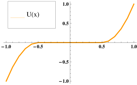
In this case the exact solution can be written down as a piecewise polynomial function:
We use the above described discretization with . The PGS algorithm produces the result given in Figure 2, and the error between numerical and exact solution (after 10 and 20 iterations) is represented in Figure 2.
Next, the table 1 we shows maximal errors between the exact and numerical solutions for this example for different numbers of discretization points and iterations ( is the maximal error while using discretization points and iterations). It is clearly visible that the error decrases along with the increase of and .
Example 2
The second example is the following 2D two-phase problem:


The numerical algorithm produces the result given in Figure 4: the surface is the solution for our problem. Figure 4 was constructed with 100 discretization points and 400 iterations. The free boundary is clearly visible in Figure 4 (the bell-shaped boundary of the white region, the zero-level set).
It is important to mention that in Figure 4 the tangential touch of two branches of the free boundary is clearly visible.
References
- [1] G. S. Weiss, An obstacle-problem-like equation with two phases: pointwise regularity of the solution and an estimate of the Hausdorff dimension of the free boundary, Interfaces Free Bound. 3 (2001) 121–128.
- [2] N. N. Uraltseva, Two-phase obstacle problem, J. Math. Sci. (New York) 106 (2001) 3073–3077. Function theory and phase transitions.
- [3] H. Shahgholian, regularity in semilinear elliptic problems, Comm. Pure Appl. Math. 56 (2003) 278–281.
- [4] E. Lindgren, H. Shahgholian, A. Edquist, On the two-phase membrane problem with coefficients below the Lipschitz threshold, Ann. Inst. H. Poincaré Anal. Non Linéaire 26 (2009) 2359–2372.
- [5] H. Shahgholian, N. Uraltseva, G. S. Weiss, The two-phase membrane problem—regularity of the free boundaries in higher dimensions, Int. Math. Res. Not. IMRN (2007) Art. ID rnm026, 16.
- [6] H. Shahgholian, G. S. Weiss, The two-phase membrane problem—an intersection-comparison approach to the regularity at branch points, Adv. Math. 205 (2006) 487–503.
- [7] J. Andersson, N. Matevosyan, H. Mikayelyan, On the tangential touch between the free and the fixed boundaries for the two-phase obstacle-like problem, Ark. Mat. 44 (2006) 1–15.
- [8] F. Bozorgnia, Numerical solutions of a two-phase membrane problem, Applied Numerical Mathematics 61 (2011) 92–107.
- [9] M. G. Crandall, P.-L. Lions, Viscosity solutions of Hamilton-Jacobi equations, Trans. Amer. Math. Soc. 277 (1983) 1–42.
- [10] M. G. Crandall, L. C. Evans, P.-L. Lions, Some properties of viscosity solutions of Hamilton-Jacobi equations, Trans. Amer. Math. Soc. 282 (1984) 487–502.
- [11] M. G. Crandall, H. Ishii, P.-L. Lions, User’s guide to viscosity solutions of second order partial differential equations, Bull. Amer. Math. Soc. (N.S.) 27 (1992) 1–67.
- [12] L. A. Caffarelli, X. Cabré, Fully nonlinear elliptic equations, volume 43 of American Mathematical Society Colloquium Publications, American Mathematical Society, Providence, RI, 1995.
- [13] H. Ishii, On the equivalence of two notions of weak solutions, viscosity solutions and distribution solutions, Funkcial. Ekvac. 38 (1995) 101–120.
- [14] A. M. Oberman, Convergent difference schemes for degenerate elliptic and parabolic equations: Hamilton-Jacobi equations and free boundary problems, SIAM J. Numer. Anal. 44 (2006) 879–895 (electronic).
- [15] N. V. Krylov, On the rate of convergence of finite-difference approximations for Bellman’s equations with variable coefficients, Probab. Theory Related Fields 117 (2000) 1–16.
- [16] B. Hu, J. Liang, L. Jiang, Optimal convergence rate of the explicit finite difference scheme for American option valuation, J. Comput. Appl. Math. 230 (2009) 583–599.
- [17] C. W. Cryer, The solution of a quadratic programming problem using systematic overrelaxation, SIAM J. Control 9 (1971) 385–392.