Constitutive relation for the system-spanning dynamically jammed region in response to impact of cornstarch and water suspensions
Abstract
We experimentally characterize the impact response of concentrated suspensions consisting of cornstarch and water. We observe that the suspensions support a large normal stress – on the order of MPa – with a delay after the impactor hits the suspension surface. We show that neither the delay nor the magnitude of the stress can yet be explained by either standard rheological models of shear thickening in terms of steady-state viscosities, or impact models based on added mass or other inertial effects. The stress increase occurs when a dynamically jammed region of the suspension in front of the impactor propagates to the opposite boundary of the container, which can support large stresses when it spans between solid boundaries. We present a constitutive relation for impact rheology to relate the force on the impactor to its displacement. This can be described in terms of an effective modulus, but only after the delay required for the dynamically jammed region to span between solid boundaries. Both the modulus and the delay are reported as a function of impact velocity, fluid height, and weight fraction. We report in a companion paper to this one on the structure of the dynamically jammed region when it spans between the impactor and the opposite boundary [1]. In a direct follow-up, we show that this constitutive model can be used to quantitatively predict, for example, the trajectory and penetration depth of the foot of a person walking or running on cornstarch and water [2].
Discontinuous Shear Thickening (DST) suspensions exhibit a remarkable effect in which they behave like typical liquids at low shear rates, but when sheared faster, resistance to flow can increase discontinuously with shear rate [3, 4]. DST suspensions can also exhibit solid-like properties such as cracking [5]. DST has been observed in a large variety of concentrated suspensions of hard, non-attractive particles, and is inferred to be a general feature of such suspensions [3, 6, 4, 7]. DST suspensions also support large stresses under impact, one example of which is the ability of a person to walk or run on the surface of a pool filled with a suspension of cornstarch and water [8, 4]. The impact response of such fluids is of practical interest for impact protection gear because of their strong response during impact while remaining fluid and flexible otherwise [9, 10]. The purpose of this paper is to obtain a constitutive relation that relates the force on an impactor to its displacement into a DST suspension. A companion paper focuses on the internal structure of the suspension that leads to the strong impact response [1]. The development of a constitutive relation may aid in the development of materials for impact protection applications.
In steady-state rheology, shear thickening is defined by a range with a positive slope in the viscosity function as a function of shear rate, where is the shear stress and the shear rate in a steady-state shear flow. The intent of such a constitutive relation is to predict flows with different forcing conditions, boundary conditions, and geometries. The constitutive relation obtained from steady-state measurements indicates that suspensions of cornstarch and water can support steady shear and normal stresses up to Pa in a shear rate range where they are shear thickening, i.e. before they become shear thinning (a negative slope of ) at higher shear rates [6]. If we try to apply this result from steady-state rheology to a person running on cornstarch and water, the predicted stress of Pa is much less than needed for a person to be supported on the surface of the fluid, based on a simple estimate of a person’s weight distributed over the surface area of a foot ( Pa). Thus, the constitutive relation obtained from steady-state rheometer experiments fails to explain the strong response to impact. It remains to be seen if our understanding of steady state DST can be extended to explain the strong impact response.
Recently an ‘added mass’ model has been developed for impact response of dense suspensions, in which a ‘dynamically jammed’ region forms ahead of the impactor in the fluid. In this localized region, the suspension moves along with the impactor like a plug [11]. The dynamically jammed region grows during the impact with a front which propagates away from the impactor [11, 12, 13]. There is a sharp velocity gradient at the front, which separates the dynamically jammed region from the surrounding fluid [12]. In a two-dimensional dry granular experiment the front velocity and width of the region with a velocity gradient both diverge at the same critical packing fraction as the viscosity curve of DST suspensions [14].
In the model for the added mass effect, the impact response of the suspension comes from an increasing suspension mass (i.e. the ‘added mass’) in the dynamically jammed region which moves with the impactor [11]. This increasing mass slows down a free-falling impactor due to conservation of momentum. This model has been confirmed to quantitatively describe the impact response of some high-speed projectiles into suspensions [11]. However, to significantly slow the impacting object by momentum conservation alone requires large masses of fluid compared to the impacting object (or similarly, large depths of the fluid compared to the object’s height). The added mass model was not quantitatively applied to other impact response problems. The regime of thin fluid layers where the added mass effect is weak is also particularly important for the related problem of impact protection applications where thin layers of protective material are desired [15, 9].
When the dynamically jammed region reaches the boundary, the stress on the impactor increases beyond the added mass effect [12]. However, it is not yet known how much more stress this boundary interaction can provide beyond the mass effect. In particular, it is not known if this can provide more stress than steady state DST, or if it can explain the strong impact response cornstarch and water is known for. We report in a companion paper to this one on the structure of the dynamically jammed region when it spans between the impactor and the opposite boundary [1]. We found that the stress increase follows immediately after particle motion is observed at the boundary opposite impact. We also observe dilation at this boundary in the same region where we find particle motion. This observation is reminiscent of soils or dense granular materials. It suggests a force transmission between particles along frictional contacts, as shear of a dense packing induces dilation as a result of particles pushing into and around each other. This suggests the dynamically jammed structure could support a normal load that is transmitted via frictional interactions across the system when the dynamically jammed region spans from the impactor to a solid stationary boundary. This assumes that the solid boundaries are much harder and have much more inertial mass than the fluid, so the solid boundary will not move or add to the mass of the dynamically jammed region. Instead, the relatively soft dynamically jammed region deforms as it is crushed between solid boundaries. We hypothesize that the system-spanning dynamically jammed region could then temporarily support a load based on its effective stiffness, perhaps strong enough to support a person running on the surface.
To obtain a constitutive relation between force and displacement, we perform impact experiments where we measure the average stress response on the impactor as a function of its displacement into the fluid. The impactor is driven far enough into a suspension to see the dynamically jammed region interacting with the boundary, in contrast to previous experiments which probed mainly the response of the bulk [11, 14, 12, 13], but not so close to the boundary to be affected by short-range boundary effects (i.e. within mm) [16]. Our experiments are at impact velocities faster than quasistatic compression, so that dynamically jammed fronts can exist, but at speeds slow enough that inertial effects are negligible [17, 18] (including added mass [11] and high Mach number effects [19, 20, 21]). This intermediate velocity regime is where the steady-state DST transition occurs (typically at flow velocities m/s in rheometers [22]), but surprisingly, systematic force measurements have not yet been reported in this regime as far as we know.
The remainder of the paper is organized as follows. The materials and methods of suspension impact experiments are explained in Sections I and II, respectively. Results of measurements of stress versus displacement of the impactor are reported in Sec. III. In Sec. IV.6, we show that the stress response to impact greatly exceeds that of previously known steady-state rheology, added mass, or inertial scalings. In Sec. IV.6 we show that the strong response occurs as soon as the dynamically jammed region spans to the opposite boundary and the added mass stops propagating with the impactor. In Sec. V we fit the stress response to obtain an averaged constitutive model for impact rheology. This includes an effective compressive modulus of the dynamically jammed region, and a delay before the modulus comes into effect due to the time it takes for the dynamically jammed region to propagate and span between solid boundaries. In a direct follow-up paper, we test this constitutive model by showing it can quantitatively explain the ability of people to walk and run on the surface of cornstarch and water [2].
I Materials
The suspensions were made of cornstarch purchased from Carolina Biological Supply, and tap water near room temperature. Measurements were made at a temperature of C, where the uncertainty represents the standard deviation from day to day. Weight fractions for cornstarch and water were measured as the weight of the cornstarch divided by the total weight of cornstarch plus water. Weight fractions of cornstarch and water are very sensitive to histories of temperature and humidity, so different data sets taken with relative humidity ranging from 8% to 54% in Sec. III are not directly comparable. To avoid misinterpretation from false comparisons, we do not report weight fractions for different experiments in this section. All samples nominally had weight fractions from 0.53 to 0.61, in a range where they all exhibited noticeable shear thickening when stirred by hand. For data sets represented in a single plot, the experiments were taken over a short enough time period to have a humidity standard deviation of 6%. We report measured weight fractions in Sec. V where systematic weight-fraction-dependent measurements were done under constant relative humidity of . Under these conditions, we found specific weight fractions such as the liquid-solid transition based on the onset of a yield stress to be reproducible within [22].
We directly measured a density of kg/m3 for a suspension at based on the volume and weight of the suspension in a graduated cylinder. If we extrapolate based on the fraction of cornstarch and water using the known density of water, the density of suspensions is not expected to deviate outside the uncertainty range for weight fractions from 0.51 to 0.63, covering our entire measurement range.
Samples were initially mixed on a vortex mixer until no dry powder chunks were observed. Before each impact measurement, samples were additionally stirred by slicing through them at least 5 times with a spatula at velocities low enough to avoid significant cracking of the suspension, and prevent large air bubbles from being trapped inside the suspension. This additional stirring helps counter any systematic effects of settling or compaction from previous experiments. This procedure produced a level of reproducibility of in stress measurements, equivalent to what we could achieve by making new samples before each measurement. If instead we did not stir between measurements or we forced air bubbles to get trapped in the suspension, the stress varied by around a factor of 2 from run to run.
II Methods

We performed experiments to visualize the top, bottom, and side boundaries of the suspension to observe the dynamically jammed region, while simultaneously measuring forces in response to impact, as shown in Fig. 1. The surface visualization results are reported in a companion paper [1]. A cylindrical aluminum impactor of diameter mm (unless otherwise noted) was pushed into a container with a square base of length mm, with the suspension filled to a height mm (unless otherwise noted). These dimensions are such that the region of interest below the impactor is far from the sidewalls of the container. The impactor surface used for experiments reported in Sec. III unintentionally had a slight wedge shape, which was angled at relative to the surface. The more quantitative experiments with controlled weight fraction reported in Sec. V were done with a leveled impactor surface. We are unaware of any effect of the misalignment on stress measurements, but to be safe we do not make direct comparison between those sections due to this misalignment and the differences in weight fractions. We used an Instron E-1000 dynamic materials tester to push the impactor into the fluid at constant velocity , while measuring the normal force on the impactor as a function of depth from the free surface of the suspension (downward positive). The nominal relative position resolution within each run is 1 m. We define and time at the top surface of the suspension, with an uncertainty of 0.5 mm. The impactor started at a height typically mm above the suspension surface and was pushed to a final position typically within of the bottom of the container. While the impactor had a set point constant impact velocity , it had to accelerate at the beginning and end of the test. This resulted in a standard deviation of the velocity of the impactor for of 11% for the data in Sec. III, and 5% for the data in Sec. V.
Since the force sensor was pushed against the impactor, the force measured by the sensor also included the force required to accelerate the mass of the impactor. To correct for this, we performed a control experiment where the impactor moved through air (i.e. with no sample). The instantaneous acceleration is obtained from twice-differentiating the position signal. We fit a linear relation between the normal force measured by the load cell and the instantaneous acceleration, where the proportionality corresponds to an effective mass of the impactor. We subtracted out the corresponding force required to accelerate the impactor equal to the effective mass times the instantaneous acceleration from later force measurements. As a result of this inertial correction, the reported force results only from the force applied by the suspension due to impact, and the overall measurement noise is reduced significantly. The force measurements are further calibrated by adding a small constant so that the load cell reads zero force when nothing is pushing against the impactor. This calibration is done separately for each measurement before the impactor hits the surface (i.e. for ). This correction amounts to less than 1% of the peak force measured.
To reduce the remaining noise in stress measurements, inertia-corrected force data is smoothed over a range of mm in to obtain a smoothed force . The average normal stress on the impactor is then given by . We calculate the noise level as the standard deviation of the smoothed stress for , and only after the velocity stayed within of the set point velocity. In the event that the velocity threshold was not reached, we calculate the standard deviation over a minimum depth range of 1 mm instead. We find is roughly proportional to such that Pa for mm/s, and reaches up to Pa for our largest mm/s. This increase is probably due to transient accelerations, which become more significant as the momentum of the impactor increases. These uncertainties amount to less than 0.14% of our maximum stress signal.
III Stress response


To characterize the stress response to impact, we performed measurements with the impactor moving into the fluid at constant velocity . These data are plotted as normal stress vs. depth in Fig. 2 for several different values of . A striking feature is that for each curve, there appears to be a delay between the point where the impactor hits the surface of the fluid (which defines depth and time ) and the depth at which there is a noticeable non-zero stress. This increase can be seen more clearly to be a sharp increase above a weak background when the same data is shown zoomed into a smaller vertical scale in Fig. 3, indicating that the scale of the stress increases by several orders of magnitude at this sharp transition. The delay will be discussed further in Sec. IV.6.
For repetitions at any given set of experimental parameters, we observed a standard deviation of in as a typical run-to-run variation. For mm/s, we occasionally measured curves where the sharp stress increase was not observed, i.e. the stress did not increase beyond a scale of Pa. This non-reproducibility may be attributable to a large natural variation inherent in the mechanical response. Such large variations have been observed for DST suspensions before, for example, even in steady-shear measurements the stress fluctuates by more than an order of magnitude over a timescale of a second [23], which is longer than our experiments for mm/s.
To determine whether the deformation is elastic or plastic, we performed extended experiments where after reaching the maximum penetration depth, we set the applied force to zero. If the deformation was mostly elastic, the impactor would have returned to near the suspension surface. Instead, the impactor remained near its maximum penetration depth, and any upward motion was limited to a few percent of the penetration depth, indicative of mostly plastic deformation. In an alternative extended experiments we set the impactor to move at velocity back to its initial position after reaching its maximum penetration depth. In this case, the system did not retrace its original stress-deformation curve as an elastic system would, rather the stress dropped quickly to zero on its return trip, again indicating the deformation is mostly plastic.
IV Comparison to existing models
Before we present a full constitutive relation, we first compare our stress measurements to existing models for steady state rheology or impact response, which allows us to establish where the smaller background signal comes from, and identify what leads to the strong stress response.
IV.1 Buoyancy
The dashed line in Fig. 3 represents the stress due to buoyancy on the impactor where kg/m3 and is the acceleration of gravity. This agrees with a good portion of the data, in particular for mm/s and for small before the onset of the sharp stress increase. This is consistent with impact experiments into pure liquids in that velocity range, as well as for granular materials with possible small corrections for friction [18]. However, This cannot explain data at larger or larger .
IV.2 Steady state rheology models
We next compare existing steady state rheology of DST to the stress in response to impact observed in Fig. 2. The maximum shear and normal stress supported by cornstarch and water in the shear thickening range under steady shear is only Pa [6]. This is still 3 orders of magnitude below the measured stress under impact. Thus, we cannot explain the large magnitude of the stress in Fig. 2 using the same viscosity function as steady state shear thickening in rheometer experiments.
The local constitutive relation inferred from steady-state shear experiments is dominated by a term where the shear stress and normal stress are related by an effective friction coefficient of order 1, mostly independent of the local shear rate [23, 6, 24, 25, 26, 27, 28, 29]. That means the local constitutive relation does not determine the magnitude of the shear and normal stresses in experiments. Rather, the maximum stress reached in DST is a function of the boundary conditions, such that the stress is limited by the stiffness of the weakest of the boundary or the particles in response to dilation [6]. In rheometer experiments, typically the weakest boundary is the surface tension of the suspension-air interface, which is what limits cornstarch and water to Pa. In cases where the stress is not limited by the suspension-air interface, the weakest stiffness could be soft walls [6] or the particle stiffness [30, 6] – the latter case has been observed in steady state flows in simulations with periodic boundary conditions [31, 24, 28], but not in hard-particle experiments. In our transient impact experiments, the strong stress response does require that the dynamically jammed region reach the boundary, so it is not a bulk response [1]. Neither do the stresses propagate throughout the entire system homogeneously to reach the suspension-air interface [1], so the suspension-air interface is not what limits the maximum stress in the impact response. There could be a different stress-limiting mechanism in response to transient impact that applies to the same local constitutive relation as steady-state flow, but this stress-limiting mechanism has not yet been identified.
This discrepancy in stress magnitudes between impact and rheometer experiments holds even if we consider other known transient effects. In rheometer experiments, the corresponding stress-strain curve during the transient (i.e. before reaching steady-state) can evolve due to transient structure formation [32, 33, 6]. The corresponding stress-strain curve exhibits a gradual increase in stress without a delay, and the stress remains mostly lower than in the steady-state, with an occasional overshoot of the steady-state by about a factor of 2. Strong fluctuations in stress have been observed around the steady state behavior [34, 35], although these have not been observed to exceed the order of magnitude of the steady-state average at the higher stress end of the shear thickening regime.
IV.3 Lubrication
Viscous drag in the small lubricated gaps between particles is another possible source of stress that is often relevant in suspensions [36]. There is an upper bound on the effective viscosity that can be obtained from such lubrication forces before continuum hydrodynamics breaks down. This occurs when the gap between solid surfaces is less than 2 liquid molecules thick [37]. The upper bound on the effective viscosity is Pas for cornstarch in water, where is the viscosity of the liquid phase, is the particle diameter, and is the liquid molecule diameter [4]. The corresponding upper bound on the stress is , which could reach only up to 2 kPa for our largest measured . This is still 3 orders of magnitude too low to explain the strong impact response of the suspension, confirming that lubrication-based hydrodynamic mechanisms cannot explain the stress increase above the background. The higher stress and effective viscosity of the measured data suggests that the particles effectively collide and more likely interact through effective solid-solid frictional interactions rather than lubrication.
IV.4 Inertial effects
At high impact velocities into fluids and granular materials, it is expected that inertial forces dominate, roughly corresponding to the force required to displace the inertial mass of fluid out of the way. The corresponding stress on the impacting object generally scales as , regardless of the internal dissipation mechanics of the material. The proportionality coefficient varies from material to material from 0.1-4 [38, 39, 40, 18, 41], and can fluctuate around a mean value [42]. The largest coefficient of 4 yields an estimate Pa in our measured range of mm/s, still 3 orders of magnitude below the measured stress response, and not even enough to hold a person’s weight. An extrapolation suggests that this would not overcome our maximum measured Pa until mm/s. High-speed impact studies of shear thickening fluids with mm/s have confirmed that inertial displacement determines the impact response [20], consistent with this extrapolation.
IV.5 Added mass
The model for the added mass effect is based on data for an object free-falling into a cornstarch and water suspension [11]. Waituakaitus & Jaeger calculated the effective stress on the impactor as the change in momentum over time per unit area , where . We can modify their model to apply to our measurements for constant velocity impacts by calculating the momentum change as the product of a constant impact velocity and a mass increasing at at rate . The growth of the added mass over time was empirically fit by a frustrum shape based on the force response on free-falling objects [11]. The added mass can be written as a function of penetration depth as
| (1) |
where is the fluid density, is the impactor diameter, and is a free parameter which represents the ratio of front velocity to impact velocity and depends on weight fraction . is obtained from the analytic derivative of Eq. 1
| (2) |
Here we have used the identity for an added mass that moves along with the impactor. This assumption is supported by the observation that the velocity of the dynamically jammed region is the same as the impactor velocity while they are in contact, corresponding to an uncompressed dynamically jammed region before it spans between solid boundaries [12]. The stress on a constant-velocity impactor from the added mass effect is then
| (3) |
While this expression can be compared directly to stress measurements, because is a free parameter, it does not indicate any upper bound on the strength of the added mass effect.
The added mass effect is in practice limited by the amount of fluid available in the suspension that can be converted to added mass. Once the dynamically jammed region reaches the boundary of the suspension opposite the impactor, the added mass can no longer propagate in the direction of the impactor, so no stress is expected from the added mass effect after this time. For a constant velocity impact, the ratio of front depth to impactor depth is the same as the ratio between front velocity to impactor velocity, so the maximum impactor depth for the added mass effect is , which can be plugged in to produce an upper bound in Eq. 3. This does not eliminate from Eq. 3, but it does indicate that when the peak stress is larger at larger , it also drops off more quickly as the dynamically jammed region reaches the opposite boundary faster. We can come up with a -independent bound on the added mass effect by realizing that the net momentum change on the impacting object comes from conservation of momentum, which is limited by the mass available in the fluid as a function of . The net work done on the impactor per unit area can be obtained from an integral of the stress-displacement curve of Eq. 3 up to depth
| (4) |
The value calculated for our experiment parameter values contributes to less than 0.6% of the integral of the measured up to the peak stress for mm/s shown in Fig. 2a, and is even smaller for lower . Since this result of Eq. 4 is independent of the only free parameter , there is no longer any flexibility in the added mass model when comparing this work per unit area. Furthermore, this -independence of the area under the curve for the added mass mechanism is independent of the specific form of the geometric factors of Eq. 3 that account for the geometry of the dynamically jammed region as prescribed by [11]. Thus, there is no way to achieve the large stress response observed in parameter range of Fig. 2 from the added mass mechanism, even by adjusting the parameter or the shape of the dynamically jammed region in the model. According to Eq. 3, the added mass effect is more relevant in impact response at larger and larger .
IV.6 Onset of stress increase above the background
So far, we have shown that the sharp increase in stress up to Pa in Fig. 2 cannot be explained by any previously known scalings, including lubrication hydrodynamics, a confining stress from surface tension, and inertial mechanisms including the added mass effect. Neither can the large scale of the stress be connected to steady-state rheology measurements which are traditionally assumed to describe flows in different geometries. Previous results indicated that a stress increase beyond the added mass effect could be a result of the dynamically jammed region reaching the opposite boundary from the impactor [12]. Here we hypothesize that the stress increase we observe up to the MPa range is the result of the this dynamically jammed region spanning between opposite boundaries, which could then support a load according to its effective stiffness. In this case, the delay depth beyond which the stress increases above the background should follow the relation . We test this hypothesis by attempting to self-consistently fit the delay depth and the contribution to the background stress from the added mass effect, which provides values of .

A first estimate of the delay depth can be obtained as the depth where first exceeds a threshold from a sum of contributions from buoyancy , the added mass , and a noise threshold , where is the standard deviation of for . This noise threshold is added so that rare fluctuations of the noise do not gives false results by exceeding the threshold prematurely. The need to minimize fluctuations here motivated the smoothing of force data explained in Sec. II. Since we hypothesize that the stress increase occurs when the dynamically jammed region first spans between solid boundaries, then we evaluate the added mass contribution from Eq. 3 when it has propagated across the system at depth . The combined stress threshold is given by
| (5) |
Since depends on , and the range where this expression is valid is up to depth , we obtain and via an iterative fit process. We start with an initial guess of [11] to calculate the threshold stress from Eq. 5. We then compare the measured stress to this threshold to obtain a depth as the first estimate of the delay depth where the threshold is first exceeded. Since this thresholding produces an overestimate, we attempt to extrapolate back to the intercept of the high-stress regime with the background signal. We do this by fitting a local slope over the range mm, or occasionally a larger range on the upper side if it resulted in a lower reduced (these larger fit ranges should give an equivalent fit with a smaller error). At low mm/s, where the background stress is dominated by bouyancy (Sec. IV.1), the added mass contribution to the stress is small compared to . In these cases we linearly extrapolate the slope down to the background from buoyancy to obtain as shown, for example, in Fig. 4a. This extrapolation helps minimize any errors introduced by the noise contribution to the threshold. Once a value of was obtained, we then adjusted to input into Eq. 5 and iterated the process until the values of and were self consistent.
For mm/s, the background stress can be described by the added mass effect. However, since the detailed contribution of the added mass effect to the stress for is not yet well-characterized, we had to consider reasonable upper and lower bounds. The fit of was extrapolated back to two different values to act as bounds on as shown in Fig. 4b. As an upper bound, the fit was extrapolated to a background given by added mass and buoyancy effects to obtain , corresponding to the added mass contribution to stress remaining constant for at the peak value reached. As a lower bound, the fit was extrapolated to a background only from buoyancy to obtain , corresponding to the added mass contribution going to zero for . Previous measurements indicate the actual response is somewhere in the range [12] where it appears that a small remaining added mass effect for is enough to keep the total stress from decaying before the boundary contribution exceeds the added mass effect. This contribution would correspond to the area in the shaded triangle in Fig. 4b. Our best estimate of the delay depth is then taken as the average of these two extrapolated bounds, with an error due to the added mass effect of . Once a value of was obtained, we adjusted and iterated the process until the values of and were self consistent.
These corrections and errors are small factors for most of the data presented in this paper. The extrapolation from the first estimate to the final value for on average results in a small correction of 18%. The error from the added mass effect is on average , and always less than 10% of , except for our largest combination of mm/s and mm (not shown in Fig. 2), where , corresponding roughly to the transition where the added mass effect becomes the dominant contribution to the total measured stress . There is also an uncertainty on of 0.5 mm due to the uncertainty on the initial position of the impactor relative to the surface of the suspension, which is usually dominant, and more so at small where this error is a significant percentage of the penetration depth. Finally, there is an uncertainty on the fit of , which is obtained by adjusting the input errors to obtain a reduced for the fit, which contributes to an error on and when extrapolated to the background. This error is only significant for a few runs at the smallest where is close to and the stress signal is weak.

We next test whether this iterative method to obtain the velocity ratio illustrated in Fig. 4 self-consistently models the added mass effect. Figure 5 show data replotted from Fig. 2, zoomed into a smaller range of and on a log-log scale for our largest to see the added mass contribution to the stress. We plot the predicted contribution from the added mass effect (Eq. 3) in Fig. 5 for each of our mm/s, using the value of obtained from the iterative method illustrated in Fig. 4, and plotting only up to in each case. It is seen that in most cases the prediction captures the scaling and magnitude the background stress, although there is a lot of variation in the data and the measurements at mm/s and mm/s fall well below the predicted added mass effect. Since the added mass contribution is less than 0.5% of the total stress measured, and the difference between the data and the model is on the same order as the measurement resolution of 1000 Pa for these data sets, these differences may be a limitation of the measurement resolution combined with the natural variability of the stress from run to run. Note that these predictions were made by fitting the onset of stress increase, not by fitting the added mass contribution to the stress directly. Overall, this agreement confirms that, within our limited resolution, the model of Waitukaitus & Jaeger [11] describes the contribution of the added mass effect to the background observed here for mm/s. This consistency check also confirms the hypothesis that the sharp stress increase occurs when the front of the added mass region reaches the solid bottom boundary.
V Constitutive model
In this section we obtain a constitutive relation that quantitatively relates the average stress on the impactor to its displacement. We base it on the observation in Fig. 2 that the relationship between stress and strain or displacement is roughly linear, suggesting we can characterize the stress response after a delay with an effective compressive modulus of the system-spanning dynamically jammed region. Mechanically, the dynamically jammed region could be much like a transient version of a soil or jammed granular material, where force would be transmitted across the system along effectively frictional contacts between particles, which is suggested by the observations of dilation from visualization of the same experiments [1]. The high stress level requires that these particle interactions are frictional rather than lubricated (as explained in Sec. IV.3). The deformation was also found to be mostly plastic (Sec. III), like a soil or granular material.
To obtain a relatively simple constitutive relation that describes the material response to impact, we report measurements of the velocity ratio between the front velocity and impact velocity which determines when the dynamically jammed region spans between solid boundaries at depth , as well as an effective compressive modulus to approximately describe the nearly linear stress increase observed afterward. Both measurements are reported over a range of impact velocities, suspension heights, and weight fractions.
V.1 Height and impact velocity dependence of the velocity ratio

The velocity ratio is calculated based on the ratio of travel distances of the front to the impactor as , where was obtained from the fit method shown in Fig. 4. These values of are shown in Fig. 6 as a function of impact velocity for different fluid heights , at the same as the data in Fig. 2. The errors plotted for are propagated from the errors on . For mm/s, the data scatter around a plateau value for different , suggesting a collapse of the data for different in this range. Fitting a constant to in the range mm/s for all , with an input error of 30% corresponding to the scatter, yields a plateau value of with a reduced , confirming consistency with a plateau. This -independent is similar to what was found by Waitukaitus & Jaeger in this velocity range [11]. The fact that -values for different collapse, at least for mm/s, confirms that in this range the delay is due to a signal propagation to the opposite boundary at constant velocity independent of in the bulk of the material,
For mm/s in Fig. 6, the values of do not collapse at different , indicating that in this range the delay depends on something other than the bulk front propagation velocity. Specifically for mm, drops off to lower values at lower impact velocities, approaching close to for mm/s. Physically, means that the dynamically jammed region is not growing or propagating faster than the impactor. An apparent slightly larger than 1 could be the result of a plug of jammed material in front of and moving at the same speed as the impactor, as suggested from the dead zone observed in particle tracking measurements [1]. Our best fit of the plateau in Fig. 6 for mm/s and mm yields , which suggests a plug height of mm. This plug height is in between the impactor diameter (12.7 mm) and the width of the dead zone with no particle flow (20 mm) observed at the bottom boundary in these experiments [1], corresponding to a plug aspect ratio around 1, which is typical for granular flows.
Assuming the values of at low are due to a plug moving with the impactor, we obtain a minimum velocity where the front of the dynamically jammed region propagates faster than the impactor. We fit a constant to for mm/s, and a power law to for mm/s at mm in Fig. 6. The crossover of these two fits shown in Fig. 6 defines a minimum velocity mm/s, where the errors on the fits are adjusted to obtain a reduced .
It is tempting to convert this critical velocity to a timescale s and relate it to other timescales observed in DST suspensions. This is consistent with a stress relaxation time ranging from 0.01 to 2 s measured in rheometer experiments [22]. Such a connection could mean that the front propagation can occur because the local shear rate around the edge of the plug exceeds the relaxation rate, allowing the dynamically jammed region to grow. It is also possible that is related to the critical shear rate from DST in rheometer measurements which varies over several orders of magnitude over the weight fraction range of DST. To test either case would require measurements of relaxation time and critical shear rate at the same weight fraction as impact experiments, measured over a range of weight fractions since the scaling of and the relaxation time are different in weight fraction. Such a study is beyond the scope of this work.
V.2 Weight fraction dependence of the velocity ratio

The values of the velocity ratio (where is obtained from the fit method shown in Fig. 4) are shown in Fig. 7 for different weight fractions with the impact velocity relatively fixed in the range 100 mm/s mm/s and mm. The value of increases with , and it appears that the values from up to the liquid-solid transition could be consistent with a plateau. The location of the liquid-solid transition at was identified as the lowest weight fraction at which a non-zero yield stress is measured in rheometer experiments, using a portion of the same samples measured simultaneously to ensure the samples were at the same weight fraction [22]. We fit a constant to data in the range , which yields a mean value with a reduced . Instead fitting to a power law in this range yields an exponent consistent with zero, confirming the data are consistent with a constant value over this fit range . The lack of divergence in approaching the liquid-solid transition sharply contrasts with a quasi-2-dimensional dry disk model which has a divergence in as [14]. We do not know if the reason for this discrepancy is due to some consequence of adding the liquid, or a difference between 2 and 3 dimensional systems, or some other physics not included in the model.
For small , approaches close to 1. We could not resolve any stress increase above the threshold in some cases for , and in all cases for for . To determine if this absence of signal is an indication of a minimum for the existence of a dynamically jammed region, or a case of the signal dropping below the resolution, we fit a linear function plus a constant to for , shown as the thin dashed line in Fig. 7. Error bars input to the fit were adjusted to a constant 27%, corresponding to a run-to-run variation to obtain a reduced . Extrapolating this fit to yields a minimum weight fraction . The agreement of the extrapolated with the consistent absence of signal at lower weight fractions confirms that this is a minimum weight fraction for the existence of a stress increase due to a dynamically jammed region spanning between solid boundaries.
We found that if the measurements of shown in Fig. 7 were repeated by another person with a nominally similar procedure with the same equipment, then the values of shifted systematically. In particular, the plateau value of changed from 8.4 to 15.7 for the two data sets. This variation in for different experimenters suggests that the front propagation behavior is sensitive to details of the sample preparation and experiment which are not yet understood or well-controlled from experiment to experiment, such as the loading and stirring of the sample. Such sensitivity may not be surprising in a system where even the run-to-run variation on repeated measurements is typically 20%-30% in most measured parameters. Considering this wider range of values of we found, the value of previously obtained from experiments with an impactor in free-fall [11] is within the variation we observed in Fig. 7. The similarity of the results suggests the model for the propagation of the dynamically jammed region proposed by Waitukaitus et al. [11] for free-falling objects also describes constant velocity impacts here.
V.3 Method to obtain the modulus
To define a compressive modulus for a disordered solid with plastic deformation and no energetically preferred height for the dynamically jammed region, and with strains up to 0.9, a linear relation between stress and strain is not appropriate. Instead we use a stress-strain relation for linear response that is continuously renormalized at each -value: . This is mathematically equivalent to calculating a modulus for a so-called ‘true strain’ [43], although our stress-strain relation is still for the averaged impact response rather than a local stress-strain relation. This approximates to a linear function for small strain after the dynamically jammed region spans between solid boundaries when . The logarithmic scaling accounts for the decreasing height of the dynamically jammed region over time. In the range , we expect the added mass effect no longer contributes to the measured stress as the dynamically jammed region has stopped growing, so we characterize the total stress by the buoyancy term plus this modulus
| (6) |
We fit Eq. 6 to stress measurements with only as a free parameter and already determined by the fit methods shown in Fig. 4. The fit range to find starts when the measured stress first exceeds the threshold stress , and the fit ends at the maximum measured stress before we stopped the impactor. Examples of fits to obtain for different are shown in Fig. 2. While the detailed stress-displacement relation is more complex than Eq. 6, this gives a simple two-parameter function for use in model predictions of the stress. The error on this model given by the root-mean-square variation of data around these fits is 10% of the maximum stress for each curve in Fig. 2. This level of error should be acceptable for many purposes since the run-to-run variation on the overall magnitude of the stress is 30%.
V.4 Impact velocity dependence of the modulus

We measured stress-displacement curves for several impact velocities , each at several different fluid heights , at the same weight fraction of the data in Fig. 2. The fit values of are shown in Fig. 8. Errors shown for include the error on the fit, and an error propagated from the error on that determines the range of the fit. The latter error can be large if either is very small so the stress signal is small, or the added mass effect is so strong that the uncertainty propagated from leads to a large uncertainty in the fit range for . For larger , some of the experiments at lower never exhibited a stress signal above the background. This is understood; assuming remains independent of , then the delay depth is expected to be larger than the machine-limited maximum penetration depth of the impactor of 55 mm.
A plateau in is observed for mm/s at each value of except for mm, consistent with the 14% run-to-run standard deviation in . For example, the solid line in Fig. 8 shows constant fit to the data for mm/s at mm. We note that the data at mm have the strongest added mass effect, in particular at mm/s the prediction for the added mass effect is 50% of the total measured stress (i.e. this is about the transition where the added mass effect overcomes the boundary effect in its contribution to the stress on the impactor). The strong added mass effect likely influences the trends observed here at large and . However, since we do not have a detailed model for the added mass effect after the collision of the dynamically jammed region with the boundary, it is difficult to account for it in detail here. The plateau in at large impact velocities is in contrast to what is expected from bulk rheology models where the shear stress remains linear in shear rate at stresses above the shear thickening regime [44], which would predict a linear relation between and in the limit of high velocity.
For smaller , the modulus scales approximately linearly with the impact velocity, as shown by the dashed line fit in Fig. 8. The non-systematic scatter in the data appears larger for mm/s, which is the same range where we found the occurrence of the sharp stress increase to be an unreliable feature from run to run. If we extrapolate the dashed line fit to lower velocities, the expected modulus becomes comparable to the background level due to buoyancy at mm/s
V.5 Geometry dependence of the modulus

To characterize whether the stress response of the dynamically jammed region scales like a bulk solid, here we show how scales with the dimensions of the system. In Fig. 8, there appears to be a systematic increase of with . To quantify this, the values of the modulus in Fig. 8 are replotted as a function of fluid height in Fig. 9 for a relatively narrow impact velocity range 100 mm/s mm/s. The dashed line shows a power law fit to these data where the input error was adjusted to 30% (about twice the typical run-to-run variation) to obtain a reduced . This yielded a power law exponent . Since is found to vary with , this indicates that is not an intrinsic material property that is independent of system size. Rather, the data are consistent with a linear scaling . Note that since , and is a constant in this parameter range, is equivalent to . This means the fit in Fig. 9 is consistent with a height-independent stiffness per unit area of the dynamically jammed region in the limit of small strain after it spans between solid boundaries (i.e. for ). If we allow for an the uncertainty in the scaling exponent of in of 0.1, propagating this error only leads to a 30% error in stress per decade of extrapolation in . This scaling implies that the mechanism that is setting the scale of the stress is coming from a bulk effect inside the suspension that is independent of the distance from the impactor to the boundary, but only after the dynamically jammed region spans between solid boundaries.
We also varied the diameter of the impactor (data not shown), and confirmed that over a range from mm, the measured modulus was consistent with no trend in over that range, within a standard deviation of 20%, within the run-to-run variation. This is consistent with the hypothesis that the modulus is independent of size. This also confirms that the shear force on the side of the impactor can be neglected in this range, as that would make a contribution to the modulus that scales as . However, for an impactor with mm, we found a modulus smaller by about a factor of 5, and a larger delay depth by about a factor of 3. This indicates the smaller impactor is in a parameter regime with very different scaling behavior than the rest of our data where is independent of . This regime at small was not studied in detail, and describing it would require a constitutive relation dependent on two spatial dimensions to include a dependence on the impactor diameter . This is beyond the scope of this paper, as the current model describes a constitutive relation averaged over the horizontal plane and is only a function of one spatial dimension ().
V.6 Weight fraction dependence of the modulus
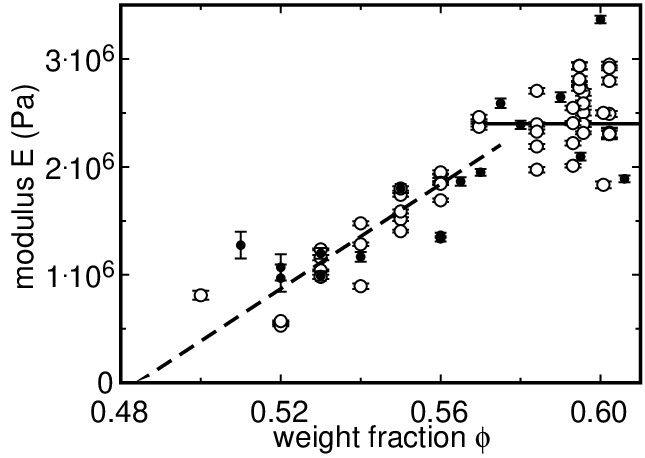
We measured the modulus for various weight fractions with the impact velocity relatively fixed in the range 100 mm/s mm/s at mm, and show the results in Fig. 10. We measured weight fractions up to the liquid-solid transition at . increases smoothly up to , followed by a plateau in . In the range , a fit to a constant yields MPa with a standard deviation of MPa, corresponding to kPa/mm. This happens to be the same range where reaches a plateau (Fig. 7). At lower , the modulus decreases. A fit of by a linear function plus a constant for shown in Fig. 10 yields an intercept where at . This is consistent with where approaches the limiting value of 1 (seen in Fig. 7) where the dynamically jammed region does not propagate. Thus it seems that the impact response gets weaker in terms of both and as the weight fraction is reduced to , although at this point the reason for this correspondence is not clear.
We found that if the measurements of as a function of shown in Fig. 10 were repeated by another person with a nominally similar procedure, the mean values of were relatively reproducible, well within each set’s standard deviation of 14%, as shown in Fig. 10. Thus, the values of seem less sensitive to the procedure than the values of .
VI Conclusions and discussion
We observed that a suspension of cornstarch and water can support a large stress in response to impact with a delay after the impactor hits the suspension surface (Fig. 2). The strong impact response occurs when the dynamically jammed region responsible for the added mass effect spans between the impactor and the opposite solid boundary [1]. The magnitude of this stress – on the order of Pa – cannot be explained by steady state rheology of DST, or impact models based on added mass or other inertial effects (Sec. III). The background stress before this delay ( Pa) can be explained by a combination of buoyancy and added mass effects (Figs. 3-5).
We used our measurements to obtain a relatively simple averaged constitutive rheology for impact response that relates the force on the impactor to its displacement. We characterized the impact response by a velocity ratio that determines when the dynamically jammed region first spans to the boundary at impactor depth (Figs. 6 and 7). The system-spanning dynamically jammed region has an effective compressive modulus for (Figs. 8, 9, and 10). The modulus depends on the fluid height , meaning that the dynamically jammed region does not have an intrinsic material modulus like typical bulk materials. Instead, we found an intrinsic stiffness per unit area to be independent of , which is independent of the distance from the boundary, although this intrinsic response only exists after the dynamically jammed region reaches the boundary. We found the values of and to be constants over a wide range of parameters: impact velocities mm/s, weight fractions (up to the liquid-solid transition), suspension heights 15 mm mm, and impactor diameters 12.7 mm mm. In this range, we find (Fig. 7), and kPa/mm (Fig. 10), where the error bars represent the large run-to-run standard deviation, including a variation for different experimenters in the case of . For smaller and , both and the velocity ratio drop off significantly. We find a minimum velocity at a given weight fraction below which the dynamically jammed region appears to act like a plug with aspect ratio near 1 that does not propagate faster than the impactor, although there is still a significant stress increase above the background. We also found a minimum weight fraction below which we did not observe any stress increase above the background at any velocity.
Despite a long-standing expectation that the impact response of cornstarch and water is related to shear thickening [30], there is still no quantitative observation that directly links the impact response of DST suspensions to their steady-state rheology. We observed dilation in the dynamically jammed region, which is a required part of the frustrated dilatancy mechanism of steady-state DST [6]. We also observed a weight fraction range of where the impact response reaches its maximum strength, in terms of modulus and the velocity ratio . The weight fraction range where in Fig. 10 and in Fig. 7 reach their maximum plateau values is the same weight fraction range where the stress-shear rate curve is discontinuous in steady-state, rotation rate-controlled measurements [22], indicating that the impact response and steady-state DST are strongest in the same weight-fraction range. At this point, these qualitative observations are the best evidence we have that the impact response and steady-state rheology might be connected, but this connection is tenuous at best. Some other comparisons that could be made to steady-state DST include the existence of a minimum weight fraction for the strong impact response above the background level (Fig. 7), and a minimum velocity for the dynamically jammed region to propagate faster than the impactor (Fig. 6). It remains to be seen if the latter is related to the critical shear rate for the onset of shear thickening in steady-state DST, or a transient relaxation time [22].
One major open question regards the physical origin of the large stress scale on the order of Pa. The observation that the modulus reaches a plateau as a function of both (Fig. 8) and (Fig. 10) is suggestive of a maximum or cutoff stress scale, analogous to the maximum stress in the shear thickening range of DST. However, this scale has not yet been explained by any models. In particular, this is 3 orders of magnitude larger than the limit from surface tension at the suspension-air interface ( Pa) that limits steady-state DST in rheometer measurements [6]. In steady-state, the stresses have time to distribute more uniformly throughout the suspension and are limited by the least stiff boundary. In contrast, the observation that the dynamically jammed structure is localized to a region below the impactor and does not need to reach the sidewalls of the system [1] suggests the normal stress transmitted along frictional interactions is limited by something inside the bulk of the suspension that exists during the transient.
Recent work proposed that the stress scale on the order of MPa could come from the pore pressure: a pressure due to the liquid flowing between the pores of the granular packing as the granular packing rearranges [45]. This model predicts a stress from pore pressure on the scale of , where the viscosity of the interstitial liquid is Pas, the permeability is , is a dimensionless coefficient of order 1, is the width of the sheared region, and we interpret as the change in weight fraction due to dilation from the initial value. If we assume [45], an estimate for a typical value of in a dilating suspension, and cm based on the size of the portion of the dynamically jammed region that is sheared at mm/s [1], then we obtain MPa. This is promising that at least pore pressure from dilation can produce a stress on the same order of magnitude as observed in Fig. 2, so the mechanism should be considered further. However, the simple model was for a uniform fluid, so could not even qualitatively predict propagation of the dynamically jammed region, and consequences of that such as the delay time or depth-dependence of the stress [45]. A complete model for the impact response should also be able to explain why the dynamically jammed region exists and propagates at all, its velocity, and the existence and values of the minimum velocity and for front propagation.
Finally, the purpose of the constitutive relation is to describe stresses, deformations, and flows of various impact-like phenomena; for examples with different forcing conditions, boundary conditions, flow geometries, and varying velocities. In a follow up paper, we show that the constitutive relation can describe the ability of people to walk and run on the surface of cornstarch and water [2]. To confirm that it is a generally useful constitutive relation requires it be tested on other transient impact-like phenomena as well. There are several phenomena of shear thickening fluids which are not explained by steady-state viscosity functions, as least in the absence of time-dependent hysteresis terms. One such phenomenon is the oscillation of the velocity of a sphere sinking in a suspension, rather than monotonically approaching a terminal velocity as it would in a generalized Newtonian fluid [46, 47, 48]. It was argued that a repeated process of jamming and unjamming of something like the dynamically jammed region could account for such oscillations [46, 47, 48]. Now we have an averaged constitutive model that includes such a process, along with a relaxation process to describe the unjamming [22]. Similarly, it was shown that the formation of stable holes in the surface of a vertically vibrated layer of a DST suspension could not be explained by a steady-state rheology in the absence of hysteresis in the constitutive relation [49]. This apparent hysteresis appears to be time-dependent when the constitutive relation is put in terms of . Alternatively, such hysteresis could come about for a history of increasing shear rate from the delay time we observed before the large stress increase. For the history of decreasing shear rate, the the time dependence may come from the relaxation time of the dynamically jammed state [22]. Finally, the observation of objects bouncing off the surface of a DST suspension remains unexplained based on steady-state or added mass models which are dissipative constitutive relations [4, 11]. The system-spanning dynamically jammed region can in principle provide some energy storage in the modulus that could possibly explain the ability of impacting objects to bounce off the surface. A detailed test of the application of the constitutive relation to these and other problems is left open for future work.
VII Acknowledgements
We thank Abe Clark, Bob Behringer, Scott Waitukaitis, Ivo Peters, Heinrich Jaeger and Madhusudhan Venkadesan for discussions and for sharing their unpublished results. This work was supported by the NSF through grant DMR 1410157.
References
- [1] B. Allen, B. Sokol, R. Maharjan, S. Mukhopadhyay, and E. Brown, “System-spanning dynamically jammed region in response to impact of cornstarch and water suspensions,” arXiv:1709.01133 (2017).
- [2] S. Mukhopadhyay, B. Allen, and E. Brown, “Testing constitutive relations by running and walking on cornstarch and water suspensions,” arXiv: (2018).
- [3] H. A. Barnes, “Shear-thickening (“dilatancy”) in suspensions of nonaggregating solid particles dispersed in newtonian liquids,” J. Rheology 33, 329 (1989).
- [4] E. Brown and H. M. Jaeger, “Shear thickening in concentrated suspensions: phenomenology, mechanisms, and relations to jamming,” Reports on Progress in Physics 77, 046602–1–23 (2014).
- [5] M. Roché, E. Myftiu, M. C. Johnston, P. Kim, and H. A. Stone, “Dynamic fracture of nonglassy suspensions,” Phys. Rev. Lett. 110, 148304 (2013).
- [6] E. Brown and H. Jaeger, “The role of dilation and confining stress in shear thickening of dense suspensions,” J. Rheology 56, 875–923 (2012).
- [7] E. Brown, N. A. Forman, C. S. Orellana, H. Zhang, B. W. Maynor, D. E. Betts, J. M. DeSimone, and H. M. Jaeger, “Generality of shear thickening in suspensions,” Nature: Materials 9, 220–224 (2010).
- [8] “https://www.youtube.com/watch?v=rumx_b_m3js, https://www.youtube.com/watch?v=thkub4ildku, http://www.wimp.com/pool-filled-with-non-newtonian-fluid-cornstarch-and-water/,” .
- [9] Y. S. Lee, E. D. Wetzel, and N.J Wagner, “The ballistic impact characteristics of kevlar-woven fabrics impregnated with a colloidal shear thickening fluid,” J. Materials Sci. 38, 2825 (2003).
- [10] http://www.d3o.com/, .
- [11] S. R. Waitukaitis and H. M. Jaeger, “Impact-activated solidification of dense suspensions via dynamic jamming fronts,” Nature 487, 205–209 (2012).
- [12] I. R. Peters and H. M. Jaeger, “Quasi-2d dynamic jamming in cornstarch suspensions: visualization and force measurements,” Soft Matter 10, 6574–6570 (2014).
- [13] Endao Han, Ivo R. Peters, and Heinrich M. Jaeger, “High-speed ultrasound imaging in dense suspensions reveals impact-activated solidification due to dynamic shear jamming,” J. Rheology 7, 12243 (2016).
- [14] S. R. Waitukaitis, L. K. Roth, V. Vitelli, and H. M. Jaeger, “Dynamic jamming fronts,” Europhysics Letters 102, 44001 (2013).
- [15] M. J. Decker, C. J. Halbach, C. H. Nam, N. J. Wagner, and E. D. Wetze, “Stab resistance of shear thickening fluid(stf)-treated fabrics,” Compos. Sci. Tech. 67, 565 (2007).
- [16] B. Liu, M. Shelley, and J. Zhang, “Focused force transmission through an aqueous suspension of granules,” Phys. Rev. Lett. 105, 188301 (2010).
- [17] R. A. Bagnold, “Experiments on a gravity-free dispersion of large solid spheres in a newtonian fluid under shear,” Proc. Royal Soc. London A: Math. and Phys. Sci. 225, 49 (1954).
- [18] A. H. Clark and R. P. Behringer, “Granular impact model as an energy-depth relation,” Europhys. Lett. 101, 64001 (2013).
- [19] A. S. Lim, S. L. Lopatnikov, N. J. Wagner, and J. W. Gillespie, “Investigating the transient response of a shear thickening fluid using the split hopkinson pressure bar technique,” Rheol. Acta 49, 879 (2010).
- [20] O. E. Petel, S. Ouellet, J. Loiseau, D. L. Frost, and A. J. Higgins, “A comparison of the ballistic performance of shear thickening fluids based on particle strength and volume fraction,” International Journal of Impact Engineering 102, 83–96 (2013).
- [21] S. Gurgen, Melih Cemal Kushan, and Weihua Li, “Shear thickening fluids in protective applications: A review,” Progress in Polymer Science (in press) (2017).
- [22] Rijan Maharjan and Eric Brown, “Giant deviation of a relaxation time from generalized newtonian theory in discontinuous shear thickening suspensions,” Phys. Rev. Fluids 2, 123301 (2017).
- [23] D. Lootens, H. vanDamme, Y. Hémar, and P. Hébraud, “Dilatant flow of concentrated suspensions of rough particles,” Phys. Rev. Lett. 95, 268302 (2005).
- [24] R. Seto, R. Mari, J. F. Morris, and M. M. Denn, “Discontinuous shear thickening of frictional hard-sphere suspensions,” Phys. Rev. Lett. 111, 218301 (2013).
- [25] N. Fernandez, R. Mani, D. Rinaldi, D. Kadau, M. Mosquet, H. Lombois-Burger, J. Cayer-Barrioz, H. J. Herrmann, N. D. Spencer, and L. Isa, “Microscopic mechanism for the shear-thickening of non-brownian suspensions,” Phys. Rev. Lett. 111, 108301 (2013).
- [26] C. Heussinger, “Shear thickening in granular suspensions: inter-particle friction and dynamically correlated clusters,” Phys. Rev. E 88, 050201(R) (2013).
- [27] John R. Royer, Daniel L. Blair, and Steven D. Hudson, “Rheological signature of frictional interactions in shear thickening suspensions,” Physical Review Letters 116 (2016).
- [28] R. Seto, G. Giusteri, and A. Mariniello, “Microstructure and thickening of dense suspensions under extensional and shear flows,” J. Fluid Mech. 825, R3 (2017).
- [29] J. Comtet, G. Chatté, A. Niguès, L. Bocquet, A. Siria, and A. Colin, “Pairwise frictional profile between particles determines discontinuous shear thickening transition in non-colloidal suspensions,” Nature Communications 8, 15633 (2017).
- [30] N.J. Wagner and J. F. Brady, “Shear thickening in colloidal dispersions,” Phys. Today, Oct. 2009 , 27–32 (2009).
- [31] M. Otsuki and H. Hayakawa, “Critical scaling near jamming transition for frictional particles,” Phys. Rev. E 83, 051301 (2011).
- [32] F. Gadala-Maria and A. Acrivos, “Shear-induced structure in a concentrated suspension of solid spheres,” J. Rheology 24, 799 (1980).
- [33] A. Fall, F. Bertrand, G. Ovarlez, and B. Bonn, “Yield stress and shear banding in granular suspensions,” Phys. Rev. Lett. 103, 178301 (2009).
- [34] D. Lootens, H. Van Damme, and P. Hébraud, “Giant stress fluctuations at the jamming transition,” Phys. Rev. Lett. 90, 178301 (2003).
- [35] S. Nagahiro and Hiizu Nakanishi, “Negative pressure in shear thickening band of a dilatant fluid,” Phys. Rev. E 94, 062614 (2016).
- [36] J. F. Brady and G. Bossis, “The rheology of concentrated suspensions of spheres in simple shear flow by numerical simulation,” J. Fluid Mech. 155, 105 (1985).
- [37] J. VanAlsten and S. Granick, “Molecular tribometry of ultrathin liquid films,” Phys. Rev. Lett. 61, 2570 (1988).
- [38] H. Schlichting, Boundary Layer Layer Theory. 4th ed. (McGraw-Hill Book Co., 1960).
- [39] William A. Allen, Earle B. Mayfield, and Harvey L. Morrison, “???dynamics of a projectile penetrating sand,” J. Applied Physics 28, 370 (1957).
- [40] P. Umbanhowar and D. I. Goldman, “Granular impact and the critical packing state,” Phys. Rev. E 82, 010301(R) (2010).
- [41] Casey Stevens Bester and Robert P. Behringer, “Collisional model of energy dissipation in three-dimensional granular impact,” Phys. Rev. E 95, 032906 (2017).
- [42] A. H. Clark, L. Kondic, and R. P. Behringer, “Particle scale dynamics in granular impact,” Phys. Rev. Lett. 109, 238302 (2012).
- [43] R. G. Budynas and J. K. Nisbett, Shigley’s Mechanical Engineering Design, 9th ed. (McGraw-Hill, 2011).
- [44] M. Wyart and M. E. Cates, “Discontinuous shear thickening without inertia in dense non-brownian suspensions,” Phys. Rev. Lett. 112, 098302 (2014).
- [45] J. John Soundar Jerome, N. Vandenberghe, and Yoel Forterre, “Unifying impacts in granular matter from quicksand to cornstarch,” Phys. Rev. Lett. 117, 098003 (2016).
- [46] S. von Kann, J. H. Snoeijer, D. Lohse, and D. van der Meer, “Non-monotonic settling of a sphere in a cornstarch suspension,” Phys. Rev. E 84, 060401 (2011).
- [47] S. von Kann, J. H. Snoeijer, and D. van der Meer, “Velocity oscillations and stop-go cycles: The trajectory of an object settling in a cornstarch suspension,” Phys. Rev. E 87, 042301 (2013).
- [48] L.O. Gálvez, S. de Beer, D. van der Meer, and A. Pons, “Dramatic effect of fluid chemistry on cornstarch suspensions: Linking particle interactions to macroscopic rheology,” Phys. Rev. E 95, 030602 (2017).
- [49] R. D. Deegan, “Stress hysteresis as the cause of persistent holes in particulate suspensions,” Phys. Rev. E 81, 036319 (2010).