Sharp interpolation inequalities for discrete operators and applications

Alexei Ilyin, Ari Laptev, Sergey Zelik Address:
Keldysh Institute of Applied Mathematics and Institute for Information Transmission Problems;
Imperial College London and Institute Mittag–Leffler;
University of Surrey, Department of Mathematics and Keldysh Institute of Applied Mathematics Email address: ilyin@keldysh.ru; a.laptev@imperial.ac.uk;
s.zelik@surrey.ac.uk

Key words and phrases:

Discrete operators, Sobolev inequality, interpolation inequalities, Green’s function, sharp constants, Lieb–Thirrng inequalities, Carlson inequality.

Abstract. We consider interpolation inequalities for imbeddings of the $l^{2}$ -sequence spaces over $d$ -dimensional lattices into the $l^{\infty}_{0}$ spaces written as interpolation inequality between the $l^{2}$ -norm of a sequence and its difference. A general method is developed for finding sharp constants, extremal elements and correction terms in this type of inequalities. Applications to Carlson’s inequalities and spectral theory of discrete operators are given.

1. Introduction

In this paper we study imbeddings of the sequence space $l^{2}(\mathbb{Z}^{d})$ into $l^{\infty}_{0}(\mathbb{Z}^{d})$ written in terms of a interpolation inequality involving the $l^{2}$ -norms both of the sequence $u\in l^{2}(\mathbb{Z}^{d})$ , and the sequence of differences $\nabla u$ , where for $u\in l^{2}(\mathbb{Z})$ and $n\in\mathbb{Z}$

\mathrm{D}u(n)=u(n+1)-u(n),

and for $u\in l^{2}(\mathbb{Z}^{d})$ and $n\in\mathbb{Z}^{d}$

\nabla u(n)=\{\mathrm{D}_{1}u(n),\dots,\mathrm{D}_{d}u(n)\},\quad\|\mathrm{D}u\|^{2}=\|\nabla u\|^{2}=\sum_{i=1}^{d}\|\mathrm{D}_{i}u\|^{2}.

Before we describe the content of the paper in greater detail we give a simple but important example [16], namely, let us prove the one-dimensional inequality

\sup_{n}u(n)^{2}\leq\|u\|\|\mathrm{D}u\|.

(1.1)

The proof repeats that in the continuous case. For an arbitrary $\gamma\in\mathbb{Z}$ we have

2u^{2}(\gamma)=\biggl(\sum_{n=-\infty}^{\gamma-1}-\sum_{n=\gamma}^{\infty}\biggr)\mathrm{D}u^{2}(n)=\\ =\biggl(\sum_{n=-\infty}^{\gamma-1}-\sum_{n=\gamma}^{\infty}\biggr)\bigl(u(n+1)\mathrm{D}u(n)+u(n)\mathrm{D}u(n)\bigr)\leq\\ \leq\sum_{n=-\infty}^{\infty}\left(|u(n+1)\mathrm{D}u(n)|+|u(n)\mathrm{D}u(n)|\right)\leq 2\|u\|\|\mathrm{D}u\|.

Below we consider separately interpolation inequalities of the form

\sup_{\mathbf{n\in\mathbb{Z}}^{d}}u(\mathbf{n})^{2}\leq\mathrm{K}_{d}(\theta)\|u\|^{2\theta}\|\nabla u\|^{2(1-\theta)},\quad 0\leq\theta\leq 1

(1.2)

in dimension $d=1,2$ and $d\geq 3$ . By notational definition $\mathrm{K}_{d}(\theta)$ is the sharp constant in this inequality. This inequality clearly holds for $\theta=1$ (with $\mathrm{K}_{d}(1)=1$ ), and if it holds for a $\theta=\theta_{*}\in[0,1)$ , then it holds for $\theta\in[\theta_{*},1]$ , when the ‘weight’ of the stronger norm $\|u\|$ is getting larger (see (1.11)).

For $d=1$ we show that (1.2) holds for $1/2\leq\theta\leq 1$ and find explicitly the corresponding sharp constant:

\mathrm{K}_{1}(\theta)=\frac{1}{2}\left(\frac{2}{\theta}\right)^{\theta}(2\theta-1)^{\theta-1/2}.

(1.3)

In the limiting case $\theta=1/2$ we have $\mathrm{K}_{1}(1/2)=1$ , and we supplement inequality (1.1) (which is, in fact, sharp) with a refined inequality

u(0)^{2}\leq\frac{1}{2}\sqrt{4-\frac{\|\mathrm{D}u\|^{2}}{\|u\|^{2}}}\,\|u\|\|\mathrm{D}u\|,

(1.4)

which for any $d\in(0,4)$ has a unique extremal sequence $u^{*}$ with $\|\mathrm{D}u^{*}\|^{2}/\|u^{*}\|^{2}=d$ .

In the 2D case (1.2) holds for $0<\theta\leq 1$ and the sharp constant is given by

\mathrm{K}_{2}(\theta)=\frac{2}{\pi}\frac{1}{\theta^{\theta}(1-\theta)^{1-\theta}}\cdot\max_{\lambda>0}\frac{\lambda^{\theta}K\left(\frac{4}{{4+\lambda}}\right)}{4+\lambda},

(1.5)

where $K$ is the complete elliptic integral of the first kind, see (3.8). The constant $\mathrm{K}_{2}(\theta)$ logarithmically tends to $\infty$ as $\theta\to 0^{+}$ , and for $\theta=0$ we have the following limiting logarithmic inequality of Brezis–Galluet type:

	$\displaystyle u(0,0)^{2}\leq\frac{1}{4\pi}\frac{\\|\nabla u\\|^{2}}{\\|u\\|^{2}}\left(1-\frac{\\|\nabla u\\|^{2}}{8\\|u\\|^{2}}\right)\left(\ln\frac{16}{\frac{\\|\nabla u\\|^{2}}{\\|u\\|^{2}}\left(8-\frac{\\|\nabla u\\|^{2}}{\\|u\\|^{2}}\right)}+\right.$		(1.6)
	$\displaystyle+\left.\ln\left(1+\ln\frac{16}{\frac{\\|\nabla u\\|^{2}}{\\|u\\|^{2}}\left(8-\frac{\\|\nabla u\\|^{2}}{\\|u\\|^{2}}\right)}\right)+2\pi\right),$		(1.6)

where the constants in front of logarithms and $2\pi$ are sharp. The inequality saturates for $u=\delta$ , otherwise the inequality is strict.

Finally, in dimension three and higher the inequality holds for the limiting exponent $\theta=0$ :

u(0)^{2}\leq\mathrm{K}_{d}\|\nabla u\|^{2},

(1.7)

where the sharp constant is given by

\mathrm{K}_{d}=\frac{1}{4(2\pi)^{d}}\int_{0}^{2\pi}\!\dots\!\int_{0}^{2\pi}\frac{dx_{1}\dots dx_{d}}{\sin^{2}\frac{x_{1}}{2}+\dots+\sin^{2}\frac{x_{d}}{2}}\,.

(1.8)

In the three dimensional case the constant $\mathrm{K}_{3}$ can be evaluated in closed form since it is expressed in terms of the so-called third Watson’s triple integral:

\mathrm{K}_{3}=\frac{1}{2}W_{S}=0.2527\dots,

(1.9)

where (see [3] and the references therein)

	$\displaystyle W_{S}:=\frac{1}{\pi^{3}}\int_{0}^{\pi}\int_{0}^{\pi}\int_{0}^{\pi}\frac{dxdydz}{3-\cos x-\cos y-\cos z}=$		(1.10)
	$\displaystyle=\frac{\sqrt{6}}{12(2\pi)^{3}}\Gamma(\tfrac{1}{24})\Gamma(\tfrac{5}{24})\Gamma(\tfrac{7}{24})\Gamma(\tfrac{11}{24}).$		(1.10)

It is natural to compare interpolation inequalities for differences and inequalities for derivatives in the continuous case. While in the continuous case the $L_{\infty}$ -norm is the strongest (at least locally), in the discrete case the $l^{1}$ -norm is the strongest. Obviously, $\|u\|_{l^{\infty}}\leq\|u\|_{l^{p}}$ for $p\geq 1$ , and therefore $\|u\|_{l^{p}}\leq\|u\|_{l^{q}}$ for $q\leq p$ :

\|u\|_{l^{p}}^{p}\leq\|u\|_{l^{\infty}}^{p-q}\|u\|_{l^{q}}^{q}\leq\|u\|_{l^{p}}^{p-q}\|u\|_{l^{q}}^{q}.

Also, unlike the continuous case, the difference operator is bounded:

\|\mathrm{D}u\|_{l^{2}(\mathbb{Z}^{d})}^{2}\leq 4d\|u\|_{l^{2}(\mathbb{Z}^{d})}^{2}.

(1.11)

Roughly speaking, the situation (at least in the one-dimensional case) is as follows. The discrete inequality (1.2) for $d=1$ holds for $\theta\in[1/2,1]$ , while the corresponding continuous inequality

\|f\|_{\infty}^{2}\leq\mathrm{C}_{1}(\theta)\|f\|^{2\theta}\|f^{\prime}\|^{2(1-\theta)},\quad f\in H^{1}(Q)

holds only for $\theta=1/2$ in case when $Q=\mathbb{R}$ , and for $\theta\in[0,1/2]$ for periodic function with zero mean, $Q=\mathbb{T}^{1}$ . Hence, it makes sense to compare the constants at a unique common point $\theta_{*}=1/2$ where both constants are equal to $1$ . For $n$ -order derivatives and differences, $n>1$ , the constants in the discrete inequalities are strictly greater than those in the continuous case, the corresponding $\theta_{*}=1-1/(2n)$ .

For example, the second-order inequality on the line $\mathbb{R}$ and the corresponding discrete inequality are as follows

	$\displaystyle\\|f\\|_{L_{\infty}(\mathbb{R})}^{2}$	$\displaystyle\leq\frac{\sqrt{2}}{\sqrt[4]{27}}\\|f\\|^{3/2}\\|f^{\prime\prime}\\|^{1/2},\quad f\in H^{2}(\mathbb{R}),$
	$\displaystyle\\|u\\|_{l^{\infty}(\mathbb{Z})}^{2}$	$\displaystyle\leq\frac{\sqrt{2}}{2}\\|u\\|^{3/2}\\|\Delta u\\|^{1/2},\quad u\in l^{2}(\mathbb{Z}).$

Both constants are sharp, the second one is strictly greater than the first. Up to a constant factor (and shift of the origin) the family of extremal functions in the first inequality is produced by scaling $x\to\lambda x$ , $\lambda>0$ of the extremal $f_{*}(x)$ , where

\int_{-\infty}^{\infty}\frac{e^{-ixy}\,dx}{x^{4}+1}=\frac{\pi\sqrt{2}}{2}f_{*}\biggl(\frac{y}{\sqrt{2}}\biggr),\qquad f_{*}(x)=e^{-|x|}(\cos x+\sin|x|),

In the discrete inequality the unique extremal sequence is $\{u_{*}(n)\}_{n=-\infty}^{\infty}$ ,

u_{*}(n)=\int_{0}^{\pi}\frac{\cos nx\,dx}{\lambda_{*}+16\sin^{4}\frac{x}{2}},\quad\text{where }\quad\lambda_{*}=\frac{16}{3};

see (5.7) for the explicit formula for $u_{*}(n)$ .

In two dimensions in the continuous case the imbedding $H^{1}\subset L_{\infty}$ holds only with a logarithmic correction term involving higher Sobolev norms (and $\theta=0$ ), which is the well-known Brezis–Gallouet inequality. On the contrary, in the $2D$ discrete case inequality (1.2) holds for $\theta\in(0,1]$ and also requires a logarithmic correction for $\theta=0$ , see (1.6).

In higher dimensional case $d\geq 3$ the imbedding $H^{1}\subset L_{\infty}$ fails at all, while inequality (1.2) holds for all $\theta\in[0,1]$ .

Next, we consider applications of discrete interpolation inequalities. Using the discrete Fourier transform and Parseval’s identities we show that each discrete interpolation inequality is equivalent to an integral Carslon-type inequality. For example, in the 1D case, setting for a function $g\in L_{2}(0,2\pi)$

I_{1}:=\int_{0}^{2\pi}g(x)dx,\ I_{2}^{2}:=\int_{0}^{2\pi}g(x)^{2}dx,\ \hat{I}_{2}^{2}:=\int_{0}^{2\pi}4\sin^{2}\tfrac{x}{2}g(x)^{2}dx,

we obtain that inequality (1.1) is equivalent to the sharp inequality

I_{1}^{2}\leq 2\pi I_{2}\hat{I}_{2},

with no extremal functions, while the refined inequality (1.4) is equivalent to the inequality

I_{1}^{2}\leq\pi\sqrt{4-\frac{\hat{I}_{2}^{2}}{{I}_{2}^{2}}}\,I_{2}\hat{I}_{2},

saturating for each $\lambda\in(-\infty,-4)\cup(0,\infty)$ at

g_{\lambda}(x)=\frac{1}{\lambda+4\sin^{2}\frac{x}{2}}\,.

Developing further this approach we prove a Sobolev $l^{q}$ -type discrete inequality for a non-limiting exponent

\|u\|_{l^{q}(\mathbb{Z}^{d})}\leq\mathrm{C}(q,d)\|\nabla u\|\quad\text{for}\quad q>{2d}/(d-2).

(1.12)

Our explicit estimate for the constant $\mathrm{C}(q,d)$ is non-sharp, moreover, it blows up as $q\to{2d}/(d-2)$ however, it is sharp in the limit $q\to\infty$ .

Finally, we apply the results on discrete inequalities to the estimates of negative eigenvalues of discrete Schrödinder operators

-\Delta-V

(1.13)

acting in $l^{2}(\mathbb{Z}^{d})$ . Here $-\Delta:=\mathrm{D}^{*}\mathrm{D}$ and $V(n)\geq 0$ . Each discrete interpolation inequality for the imbedding into $l^{\infty}(\mathbb{Z}^{d})$ produces by the method of [7] a collective inequality for families of orthonormal sequences, which, in turn, is equivalent to a Lieb-Thirring estimate for the negative trace. For example, we deduce from (1.7) the estimate

\sum_{\lambda_{j}<0}|\lambda_{j}|\leq\frac{\mathrm{K}_{d}}{4}\sum_{\alpha\in\mathbb{Z}^{d}}V^{2}(\alpha),

which holds for $d\geq 3$ .

We finally point out that in the continuous case the classical Lieb–Thirring inequality for the negative trace of operator (1.13) in $L_{2}(\mathbb{R}^{d})$ is as follows (see [14], [13], [6])

\sum_{\lambda_{j}<0}|\lambda_{j}|\leq\mathrm{L}_{1,d}\int_{\mathbb{R}^{d}}V^{1+d/2}(x)dx.

2. 1D case

Since $u_{n}\to 0$ as $|n|\to\infty$ , without loss of generality we can assume that $\sup_{n}u(n)^{2}=u(0)^{2}$ .

We consider a more general problem of finding sharp constants, existence of extremals and possibly correction terms in the inequalities of the type

u(0)^{2}\leq\mathrm{K}_{1}(\theta)\|u\|^{2\theta}\|\mathrm{D}u\|^{2(1-\theta)},\quad 0\leq\theta\leq 1,

(2.1)

including, to begin with, the problem of finding those $\theta$ for which (2.1) holds at all. Here

\|u\|^{2}=\sum_{k=-\infty}^{\infty}u(k)^{2},\quad\|\mathrm{D}u\|^{2}=\sum_{k=-\infty}^{\infty}\mathrm{D}u(k)^{2}.

Since $|a-b|\geq||a|-|b||$ , we have

\|\mathrm{D}|u|\|\leq\|\mathrm{D}u\|,\quad\text{where}\quad|u|:=\{|u(n)|\}_{n=-\infty}^{\infty},

(2.2)

and we could have further reduced our treatment to the case when $u(n)\geq 0$ . However, we shall be dealing below with a more general problem (2.4) which has both sing-definite and non-sign-definite extremals. We have the following ‘reverse’ Poincare inequality:

\|\mathrm{D}u\|^{2}\leq\left\{\begin{array}[]{ll}2\|u\|^{2},&u\hbox{ is sign definite;}\\ 4\|u\|^{2},&\hbox{otherwise.}\end{array}\right.

(2.3)

The adjoint to $\mathrm{D}$ is the operator:

\mathrm{D}^{*}u(n)=-(u(n)-u(n-1)),

and

\mathrm{D}^{*}\mathrm{D}u(n)=\mathrm{D}\mathrm{D}^{*}u(n)=-\bigl(u(n+1)-2u(n)+u(n-1)\bigr).

To find the sharp constant $\mathrm{K}_{1}(\theta)$ in (2.1) we consider a more general problem: find $\mathbb{V}(d)$ , where $\mathbb{V}(d)$ is the solution of the following maximization problem:

\mathbb{V}(d):=\sup\bigl\{u(0)^{2}:\ u\in l^{2}(\mathbb{Z}),\ \|u\|^{2}=1,\ \|\mathrm{D}u\|^{2}=d\bigr\},

(2.4)

where $0<d<4$ .

Its solution is found in terms of the Green’s function of the corresponding second-order self-adjoint positive operator, see [18], [1]. The spectrum of the operator $-\Delta=\mathrm{D}^{*}\mathrm{D}$ is the closed interval $[0,4]$ , and we set

\mathbb{A}(\lambda)=\left\{\begin{array}[]{ll}\phantom{-}\mathrm{D}^{*}\mathrm{D}+\lambda,&\hbox{for $\lambda>0$;}\\ -\mathrm{D}^{*}\mathrm{D}-\lambda,&\hbox{for $\lambda<-4$.}\end{array}\right.

(2.5)

Then $\mathbb{A}(\lambda)$ is positive definite

(\mathbb{A}(\lambda)u,u)=\left\{\begin{array}[]{ll}\phantom{-}\|\mathrm{D}u\|^{2}+\lambda\|u\|^{2}>\lambda\|u\|^{2},&\hbox{for $\lambda>0$;}\\ -\|\mathrm{D}u\|^{2}-\lambda\|u\|^{2}>(-\lambda-4)\|u\|^{2},&\hbox{for $\lambda<-4$.}\end{array}\right.

Let $\delta$ be the delta-sequence: $\delta(0)=1$ , $\delta(n)=0$ for $n\neq 0$ , and let $G_{\lambda}=\{G_{\lambda}(n)\}_{n=-\infty}^{\infty}\in l^{2}(\mathbb{Z})$ be the Green’s function of operator (2.5), that is, the solution of the equation:

\mathbb{A}(\lambda)G_{\lambda}=\delta.

(2.6)

Then we have by the Cauchy–Schwartz inequality

	$\displaystyle u(0)^{2}=(\delta,u)^{2}=(\mathbb{A}(\lambda)G_{\lambda},u)^{2}=$		(2.7)
	$\displaystyle=(\mathbb{A}(\lambda)^{1/2}G_{\lambda},\mathbb{A}(\lambda)^{1/2}u)^{2}\leq(\mathbb{A}(\lambda)G_{\lambda},G_{\lambda})(\mathbb{A}(\lambda)u,u)=$
	$\displaystyle=G_{\lambda}(0)(\mathbb{A}(\lambda)u,u).$

Furthermore, this inequality is sharp and turns into equality if and only if $u=\mathrm{const}\cdot G_{\lambda}$ .

We find in Lemma 2.2 explicit formulas for $\mathbb{V}(d)$ and $G_{\lambda}(n)$ . Nevertheless, we now independently prove the following two symmetry properties of $\mathbb{V}(d)$ and $G_{\lambda}(n)$ , especially since their counterparts will be useful in the two-dimensional case below.

Proposition 2.1.

For $d\in(0,4)$

\mathbb{V}(d)=\mathbb{V}(4-d).

(2.8)

For $\lambda>0$ and $n\in\mathbb{Z}$

0<G_{\lambda}(n)=(-1)^{|n|}G_{-4-\lambda}(n).

(2.9)

Proof.

For $u\in l^{2}(\mathbb{Z})$ we define the orthogonal operator $T$

Tu=u^{\star}:=\{(-1)^{|n|}u(n)\}_{n=-\infty}^{\infty}.

Then clearly $\|u\|^{2}=\|u^{\star}\|^{2}$ and, in addition,

\|\mathrm{D}u^{\star}\|^{2}=4\|u\|^{2}-\|\mathrm{D}u\|^{2}.

(2.10)

Therefore if for a fixed $d$ and $u=u_{d}$ we have

\mathbb{V}(d)=u(0)^{2},\quad\|u\|^{2}=1\quad\text{and}\quad\|\mathrm{D}u\|^{2}=d,

then for $u^{*}=Tu$ it holds

u^{\star}(0)^{2}=u(0)^{2}=\mathbb{V}(d),\quad\|u^{\star}\|^{2}=1\quad\text{and}\quad\|\mathrm{D}u^{\star}\|^{2}=4-d,

which gives that $\mathbb{V}(4-d)\geq\mathbb{V}(d)$ . However, the strict inequality here is impossible, since otherwise by repeating this procedure we would have found that $\mathbb{V}(d)>\mathbb{V}(d)$ . This proves (2.8).

Turning to (2.9) we note that $T^{-1}=T^{*}=T$ and we see from (2.10) that

(\mathrm{D}^{*}\mathrm{D}u,u)=(T(-\mathrm{D}^{*}\mathrm{D}+4)Tu,u),

and, consequently,

\mathrm{D}^{*}\mathrm{D}=T(-\mathrm{D}^{*}\mathrm{D}+4)T.

Therefore, if for $\lambda>0$ , $G_{\lambda}$ solves

\mathbb{A}(\lambda)G_{\lambda}=(\mathrm{D}^{*}\mathrm{D}+\lambda)G_{\lambda}=\delta,

then

T(-\mathrm{D}^{*}\mathrm{D}+4+\lambda)TG_{\lambda}=\delta.

Since $T^{-1}\delta=\delta$ , using definition (2.5) we obtain

(-\mathrm{D}^{*}\mathrm{D}+4+\lambda)TG_{\lambda}=\mathbb{A}(-4-\lambda)TG_{\lambda}=\delta,

which gives

TG_{\lambda}=G_{-4-\lambda},

and proves the equality in (2.9).

It remains to show that for $\lambda>0$ $G_{\lambda}(n)>0$ for all $n$ . Since $\mathbb{A}(\lambda)$ is positive definite, it follows that $G_{\lambda}(0)=(\mathbb{A}(\lambda)G_{\lambda},G_{\lambda})>0$ . We use the maximum principle and suppose that for some $n\neq 1$ , $G_{\lambda}(n)<0$ . Since $G_{\lambda}(n)\to 0$ as $n\to\infty$ and $G_{\lambda}(0)>0$ , it follows that $G_{\lambda}$ attains a global strictly negative minimum at some point $n>1$ (the case $n<-1$ is similar). Then the sum of the first three terms in (2.20) is non-positive and the fourth term is strictly negative, which contradicts $\delta(n)=0$ . This proves that $G_{\lambda}(n)\geq 0$ for all $n$ . Finally, to prove strict positivity, we suppose that $G_{\lambda}(n)=0$ for some $n>1$ . Then we see from (2.20) that $G_{\lambda}(n-1)+G_{\lambda}(n+1)=0$ , and what has already been proved gives $G_{\lambda}(n-1)=G_{\lambda}(n+1)=0$ . Repeating this we reach $n=1$ giving that $G_{\lambda}(0)=0$ , which is a contradiction. ∎

To denote the three norms of $G_{\lambda}$ we set

f(\lambda):=G_{\lambda}(0),\quad g(\lambda):=\|G_{\lambda}\|^{2},\quad h(\lambda):=\|\mathrm{D}G_{\lambda}\|^{2}.

(2.11)

Lemma 2.1.

The functions $f$ , $g$ and $h$ satisfy

g(\lambda)=-\mathrm{sign}(\lambda)f^{\prime}(\lambda),\ \ h(\lambda)=\mathrm{sign}(\lambda)(f(\lambda)+\lambda f^{\prime}(\lambda)).

(2.12)

Proof.

Let $\lambda>0$ . Then $\mathbb{A}(\lambda)=\mathrm{D}^{*}\mathrm{D}+\lambda$ . Taking the scalar product of (2.6) with $G_{\lambda}$ we have

f(\lambda)=G_{\lambda}(0)=\|\mathrm{D}G_{\lambda}\|^{2}+\lambda\|G_{\lambda}\|^{2}=h(\lambda)+\lambda g(\lambda).

(2.13)

Differentiating this formula with respect to $\lambda$ we obtain

f^{\prime}(\lambda)=2(\mathbb{A}(\lambda)G^{\prime}_{\lambda},G_{\lambda})+g(\lambda)=\\ =-2(G_{\lambda},G_{\lambda})+g(\lambda)=-g(\lambda),

(2.14)

where we used that $G_{\lambda}+\mathbb{A}(\lambda)G^{\prime}_{\lambda}=0$ , which, in turn, follows from (2.6). The case $\lambda<-4$ is treated similarly taking into account that now $\mathbb{A}(\lambda)=-\mathrm{D}^{*}\mathrm{D}-\lambda$ . ∎

Corollary 2.1.

The function $d(\lambda)$ defined as follows

d(\lambda):=\frac{\|\mathrm{D}G_{\lambda}\|^{2}}{\|G_{\lambda}\|^{2}}=\frac{h(\lambda)}{g(\lambda)}

(2.15)

satisfies the functional equation

d(-4-\lambda)=4-d(\lambda).

(2.16)

Proof.

It follows from (2.9) and (2.11) that

f(-4-\lambda)=f(\lambda).

Hence, $f^{\prime}(\lambda)=-f^{\prime}(-4-\lambda)$ and we obtain from (2.12)

	$\displaystyle d(-4-\lambda)=\frac{h(-4-\lambda)}{g(-4-\lambda)}=\frac{f(-4-\lambda)+(-4-\lambda)f^{\prime}(-4-\lambda)}{-f^{\prime}(-4-\lambda)}=$
	$\displaystyle=\frac{f(\lambda)+(4+\lambda)f^{\prime}(\lambda)}{f^{\prime}(\lambda)}=\frac{f(\lambda)+\lambda f^{\prime}(\lambda)}{f^{\prime}(\lambda)}+4=4-d(\lambda).$

∎

Next, we find explicit formulas for $f$ , $g$ and $h$ .

Lemma 2.2.

The Green’s function $G_{\lambda}$ belongs to $l^{2}(\mathbb{Z})$ , and both for $\lambda\in(-\infty,-4)$ and $\lambda\in(0,\infty)$

f(\lambda)=\frac{1}{\sqrt{\lambda(\lambda+4)}},\ g(\lambda)=\frac{\lambda+2}{(\lambda+4)\sqrt{\lambda^{3}(\lambda+4)}},\ h(\lambda)=\frac{2}{\sqrt{\lambda(\lambda+4)^{3}}}\,.

(2.17)

Furthermore, the elements $G_{\lambda}(n)$ can be found explicitly: for $\lambda>0$

G_{\lambda}(n)=\frac{1}{\pi}\ \int_{0}^{\pi}\frac{\cos nx\,dx}{\lambda+4\sin^{2}\frac{x}{2}}=\frac{1}{\sqrt{\lambda(\lambda+4)}}\left(\frac{\lambda+2-\sqrt{\lambda(\lambda+4)}}{2}\right)^{|n|}\,,

(2.18)

for $\lambda<-4$

G_{\lambda}(n)=-\frac{1}{\pi}\ \int_{0}^{\pi}\frac{\cos nx\,dx}{\lambda+4\sin^{2}\frac{x}{2}}=\frac{1}{\sqrt{\lambda(\lambda+4)}}\left(\frac{\lambda+2+\sqrt{\lambda(\lambda+4)}}{2}\right)^{|n|}\,.

(2.19)

Proof.

In view of (2.12), for the proof of (2.17) it suffices to find only $f(\lambda)=G_{\lambda}(0)$ . We consider two cases: $\lambda>0$ and $\lambda<-4$ . For $\lambda>0$ the sequence $G_{\lambda}$ solves (2.6), which takes the form $(\mathrm{D}^{*}\mathrm{D}+\lambda)G_{\lambda}=\delta$ , or component-wise

-G_{\lambda}(n+1)+2G_{\lambda}(n)-G_{\lambda}(n-1)+\lambda G_{\lambda}(n)=\delta(n).

(2.20)

We multiply each equation by $e^{inx}$ and sum the results from $n=-\infty$ to $\infty$ . Setting

\widehat{g}_{\lambda}(x):=\sum_{n=-\infty}^{\infty}G_{\lambda}(n)e^{inx},

we obtain

-\sum_{n=-\infty}^{\infty}e^{inx}G_{\lambda}(n+1)+(2+\lambda)\sum_{n=-\infty}^{\infty}e^{inx}G_{\lambda}(n)-\sum_{n=-\infty}^{\infty}e^{inx}G_{\lambda}(n-1)=1

	$\displaystyle 1=\widehat{g}_{\lambda}(x)(\lambda-e^{-ix}+2-e^{ix}))=$
	$\displaystyle=\widehat{g}_{\lambda}(x)\bigl(\lambda-(e^{ix/2}-e^{-ix/2})^{2}\bigr)=\widehat{g}_{\lambda}(x)\left(\lambda+4\sin^{2}\frac{x}{2}\right),$

which gives $\widehat{g}_{\lambda}(x)=1/(\lambda+4\sin^{2}\frac{x}{2})$ .

In the case when $\lambda<-4$ equation (2.6) becomes $(\mathrm{D}^{*}\mathrm{D}+\lambda)G_{\lambda}=-\delta$ and we merely have to change the sign of $\widehat{g}_{\lambda}(x)$ and we obtain:

\widehat{g}_{\lambda}(x)=\left\{\begin{array}[]{ll}\phantom{-}\frac{1}{\lambda+4\sin^{2}\frac{x}{2}},&\lambda>0;\\ -\frac{1}{\lambda+4\sin^{2}\frac{x}{2}},&\lambda<-4,\end{array}\right.

(2.21)

and

G_{\lambda}(n)=\frac{1}{2\pi}\int_{-\pi}^{\pi}\widehat{g}_{\lambda}(x)\cos nx\,dx.

(2.22)

Since $\widehat{g}_{\lambda}\in L_{2}(0,2\pi)$ , it follows that $G_{\lambda}\in l^{2}(\mathbb{Z})$ .

Using the integral

\int_{-\pi}^{\pi}\frac{dx}{b+\sin^{2}\frac{x}{2}}=\left\{\begin{array}[]{ll}\phantom{-}\frac{2\pi}{\sqrt{b(b+1)}},&b>0;\\ -\frac{2\pi}{\sqrt{b(b+1)}},&b<-1.\end{array}\right.

(2.23)

we finally obtain both for $\lambda>0$ , and $\lambda<-4$

f(\lambda)=G_{\lambda}(0)=\frac{1}{2\pi}\int_{-\pi}^{\pi}\widehat{g}_{\lambda}(x)dx=\frac{1}{\sqrt{\lambda(\lambda+4)}}\,.

(2.24)

Finally, to obtain the explicit formula (2.18) (which will not be used below) we observe that the equation (2.20) for positive (and negative) $n$ is a homogeneous linear recurrence relation with constant coefficients. The characteristic equation is

q^{2}-(2+\lambda)q+1=0

with roots

	$\displaystyle q_{1}(\lambda)$	$\displaystyle=\frac{\lambda+2-\sqrt{\lambda(\lambda+4)}}{2},\quad 0<q_{1}(\lambda)<1\ \text{ for}\ \lambda>0,$
	$\displaystyle q_{2}(\lambda)$	$\displaystyle=\frac{\lambda+2+\sqrt{\lambda(\lambda+4)}}{2},\quad-1<q_{2}(\lambda)<0\ \text{ for}\ \lambda<-4.$

For $\lambda>0$ the general $l^{2}$ -solution of (2.20) is $G_{\lambda}(n)=c_{1}(\lambda)q_{1}(\lambda)^{n}$ for $n>0$ and $G_{\lambda}(n)=c_{2}(\lambda)q_{1}(\lambda)^{|n|}$ for $n<0$ . Since we already know that $G_{\lambda}(n)=G_{\lambda}(-n)$ , it follows that $c_{1}(\lambda)=c_{2}(\lambda)=:a(\lambda)$ . Substituting $G_{\lambda}(n)=a(\lambda)q_{1}(\lambda)^{|n|}$ into (2.20) with $n=0$ we obtain $-2a(\lambda)q_{1}(\lambda)+(2+\lambda)a(\lambda)=1$ , which gives

a(\lambda)=\frac{1}{2+\lambda-2q_{1}(\lambda)}=\frac{1}{\sqrt{\lambda(\lambda+4)}}\,

and proves (2.18). The proof of (2.19) in the case $\lambda<-4$ is totally similar, we only have to use the second root $q_{2}(\lambda)$ with $|q_{2}(\lambda)|<1$ .

We finally point out that the equality (2.9) can now be also verified by a direct calculation: $q_{2}(-4-\lambda)=-q_{1}(\lambda)$ . ∎

We can now give the solution to the problem (2.4).

Theorem 2.1.

For any $0<d<4$ the solution of the maximization problem (2.4) is given by

\mathbb{V}(d)=\frac{1}{2}\sqrt{d(4-d)}.

(2.25)

The supremum in (2.4) is the maximum that is attained at a unique sequence $u^{*}_{\lambda(d)}=\|G_{\lambda(d)}\|^{-1}G_{\lambda(d)}$ , where

\lambda(d)=\frac{2d}{{2-d}}

(2.26)

for $d\neq 2$ ; for $d=2$ , $u^{*}=\delta$ .

Proof.

It follows from (2.7) that for any $u\in l^{2}(\mathbb{Z})$

u(0)^{2}\leq G_{\lambda}(0)(\mathbb{A}(\lambda)u,u),

and, furthermore, for

u_{\lambda}^{*}:=\frac{1}{\|G_{\lambda}\|}\cdot G_{\lambda}

with $\|u_{\lambda}^{*}\|^{2}=1$ the above inequality turns into equality.

Next, using (2.17) we find the formula for the function $d(\lambda)$ defined in (2.15)

d(\lambda)=\frac{\|\mathrm{D}G_{\lambda}\|^{2}}{\|G_{\lambda}\|^{2}}=\frac{h(\lambda)}{g(\lambda)}=\frac{2\lambda}{2+\lambda}\,,\qquad d:\left\{\begin{array}[]{ll}(0,\infty)\to(0,2),\\ (-\infty,-4)\to(2,4).\end{array}\right.

The inverse function $\lambda(d)$ is given by (2.26) and with this $\lambda(d)$ we have

\frac{\|\mathrm{D}u_{\lambda(d)}^{*}\|^{2}}{\|u_{\lambda(d)}^{*}\|^{2}}=\frac{h(\lambda(d))}{g(\lambda(d))}=\frac{2\lambda(d)}{2+\lambda(d)}=d\,.

Therefore $u_{\lambda(d)}^{*}$ is the extremal sequence in (2.4) and its solution is

\mathbb{V}(d)=u_{\lambda(d)}^{*}(0)^{2}=\frac{f(\lambda(d))^{2}}{g(\lambda(d))}=\frac{1}{2}\sqrt{d(4-d)}.

∎

Remark 2.1.

It is worth pointing out that in accordance with Proposition 2.1 and Corollary 2.1 we directly see here that $\mathbb{V}(d)=\mathbb{V}(4-d)$ and $d(-4-\lambda)=4-d(\lambda)$ . For the inverse function $\lambda(d)$ we have the functional equation $\lambda(4-d)=-4-\lambda(d)$ .

Corollary 2.2.

For any $u\in l^{2}(\mathbb{Z})$ inequality (1.1) holds, the constant $1$ is sharp and no extremals exist. The following refined inequality holds:

u(0)^{2}\leq\frac{1}{2}\sqrt{4-\frac{\|\mathrm{D}u\|^{2}}{\|u\|^{2}}}\,\|u\|\|\mathrm{D}u\|.

(2.27)

For any $0<d<4$ the inequality saturates for $u^{*}_{\lambda(d)}=G_{\lambda(d)}$ , where $\lambda(d)=\frac{2d}{{2-d}}$ (see (2.26)) with $\|\mathrm{D}u^{*}_{\lambda(d)}\|^{2}/\|u^{*}_{\lambda(d)}\|^{2}=d$ . For $d=2$ , $u^{*}=\delta$ .

Proof.

Inequality (2.27) follows from (2.25) by homogeneity.

Since $\mathbb{V}(d)<\sqrt{d}$ , we obtain inequality (1.1), and since $\mathbb{V}(d)/\sqrt{d}\to 1$ as $d\to 0$ the constant $1$ is sharp. In view of the refined inequality (2.27) there can be no extremals in the original inequality (1.1). ∎

We now consider (2.1) for $\theta\neq 1/2$ .

Theorem 2.2.

Inequality (2.1) holds only for $1/2\leq\theta\leq 1$ . The sharp constant $\mathrm{K}_{1}(\theta)$ is

\mathrm{K}_{1}(\theta)=\frac{1}{2}\left(\frac{2}{\theta}\right)^{\theta}(2\theta-1)^{\theta-1/2}.

(2.28)

For each $1/2<\theta\leq 1$ there exists a unique extremal sequence.

Proof.

The proof is similar to the proof of Theorem 2.5 in [18] where the classical Sobolev spaces were considered. For convenience we include some details.

We first observe that inequality (2.1) cannot hold for $\theta<1/2$ , since otherwise we would have found that $\mathbb{V}(d)\leq cd^{\eta}$ , $\eta=1-\theta>1/2$ , a contradiction with (2.25): $\mathbb{V}(d)\sim d^{1/2}$ as $d\to 0$ .

The case $\theta=1/2$ was treated above and we assume in what follows that $\theta>1/2$ . We set

\lambda:=\frac{\theta}{1-\theta}\frac{\|\mathrm{D}u\|^{2}}{\|u\|^{2}}.

(2.29)

Then, using (2.7), we have

	$\displaystyle u(0)^{2}\leq G_{\lambda}(0)\\|u\\|^{2}\left(\frac{\\|\mathrm{D}u\\|^{2}}{\\|u\\|^{2}}+\lambda\right)=\frac{1}{\theta}G_{\lambda}(0)\lambda^{\theta}\lambda^{1-\theta}\\|u\\|^{2}=$		(2.30)
	$\displaystyle=\frac{1}{\theta}\lambda^{\theta}G_{\lambda}(0)\left(\frac{\theta}{1-\theta}\frac{\\|\mathrm{D}u\\|^{2}}{\\|u\\|^{2}}\right)^{1-\theta}\\|u\\|^{2}=$
	$\displaystyle=\frac{1}{\theta^{\theta}(1-\theta)^{1-\theta}}\cdot\lambda^{\theta}G_{\lambda}(0)\\|u\\|^{2\theta}\\|\mathrm{D}u\\|^{2(1-\theta)}\leq$
	$\displaystyle\leq\frac{1}{\theta^{\theta}(1-\theta)^{1-\theta}}\cdot\sup_{\lambda>0}\bigg\{\lambda^{\theta}G_{\lambda}(0)\bigg\}\,\\|u\\|^{2\theta}\\|\mathrm{D}u\\|^{2(1-\theta)}=$
	$\displaystyle=\mathrm{K}_{1}(\theta)\\|u\\|^{2\theta}\\|\mathrm{D}u\\|^{2(1-\theta)}.$

We have taken into account in the last equality that

G_{\lambda}(0)=f(\lambda)=\frac{1}{\sqrt{\lambda(\lambda+4)}}.

Hence, the supremum in the above formula is a (unique) maximum on $\lambda\in\mathbb{R}^{+}$ of the function

\lambda^{\theta}f(\lambda)=\frac{\lambda^{\theta-1/2}}{\sqrt{\lambda+4}}

attained at $\lambda_{*}=(4\theta-2)/(1-\theta)$ , which gives (2.28). To see that the constant $\mathrm{K}_{1}(\theta)$ is sharp we use that $\frac{d}{d\lambda}(\lambda^{\theta}f(\lambda))|_{\lambda=\lambda_{*}}=0$ , and $\lambda_{*}f^{\prime}(\lambda_{*})+\theta f(\lambda_{*})=0$ . In view of (2.12) this gives

d_{*}:=d(\lambda_{*})=\frac{\|\mathrm{D}G_{\lambda_{*}}\|^{2}}{\|G_{\lambda_{*}}\|^{2}}=\frac{h(\lambda_{*})}{g(\lambda_{*})}=-\frac{f(\lambda_{*})+\lambda_{*}f^{\prime}(\lambda_{*})}{f^{\prime}(\lambda_{*})}=\frac{1-\theta}{\theta}\lambda_{*}.

Hence (2.29) is satisfied for $u_{*}=G_{\lambda_{*}}$ the two inequalities in (2.30) become equalities, and $u_{*}$ is the unique extremal. ∎

Refer to caption — Figure 1. Graphs of sharp constants in one-dimensional first-order inequalities on complementary intervals: periodic functions (left) (5.18), discrete case (right) (2.28).

The graph of the function $\mathrm{K}_{1}(\theta)$ is shown in Fig.1 on the right. Here $\mathrm{K}_{1}(1/2)=1$ corresponds to (1.1), and $\mathrm{K}_{1}(1)=1$ corresponds to the trivial inequality $u(0)^{2}\leq\|u\|^{2}$ with extremal $u=\delta$ .

Remark 2.2.

In this theorem we do not use the formula (2.25) for $\mathbb{V}(d)$ . However, if we do, then finding $\mathrm{K}_{1}(\theta)$ for $\theta\in[1/2,1]$ becomes very easy. In fact, by the definition of $\mathbb{V}(d)$ and homogeneity, $\mathrm{K}_{1}(\theta)$ is the smallest constant for which $\mathbb{V}(d)\leq\mathrm{K}_{1}(\theta)d^{1-\theta}$ for all $d\in[0,4]$ . Therefore

\mathrm{K}_{1}(\theta)=\max_{d\in[0,4]}\mathbb{V}(d)/d^{1-\theta}=\max_{d\in[0,4]}\frac{1}{2}d^{\theta-1/2}(4-d)^{1/2}=\text{r.h.s.}\eqref{K(theta)}.

The corresponding $d_{*}=(4\theta-2)/\theta\leq 2$ and $\lambda(d_{*})>0$ , see (2.26). This also explains why the region of negative $\lambda$ does not play a role in Theorem 2.2.

3. 2D case

In this section we consider the two-dimensional inequalities

u(0,0)^{2}\leq\mathrm{K}_{2}(\theta)\|u\|^{2\theta}\|\nabla u\|^{2(1-\theta)},\quad 0\leq\theta\leq 1,

(3.1)

and address the same problems as in the previous section.

We set

\Delta=-\mathrm{D}_{1}^{*}\mathrm{D}_{1}-\mathrm{D}_{2}^{*}\mathrm{D}_{2}.

Then $(-\Delta u,u)=\|\nabla u\|^{2}\leq 8\|u\|^{2}$ for $u\in l_{2}(\mathbb{Z}^{2})$ . As in the 1D case we shall be dealing with the following extremal problem:

\mathbb{V}(d):=\sup\bigl\{u(0,0)^{2}:\ u\in l^{2}(\mathbb{Z}^{2}),\ \|u\|^{2}=1,\ \|\mathrm{D}u\|^{2}=d\bigr\},

(3.2)

where $0<d<8$ .

The resolvent set of $-\Delta+\lambda$ is $(-\infty,-8)\cup(0,\infty)$ and as before we consider the positive self-adjoint operator operator

\mathbb{A}(\lambda)=\left\{\begin{array}[]{ll}-\Delta+\lambda,&\hbox{for $\lambda>0$;}\\ \phantom{-}\Delta-\lambda,&\hbox{for $\lambda<-8$.}\end{array}\right.

Our main goal is to find the Green’s function of it:

\mathbb{A}(\lambda)G_{\lambda}=\delta,

(3.3)

more precisely, $G_{\lambda}(0,0)$ .

Proposition 3.1.

For $d\in(0,8)$

\mathbb{V}(d)=\mathbb{V}(8-d).

(3.4)

For $\lambda>0$ and $(n,m)\in\mathbb{Z}^{2}$

0<G_{\lambda}(n,m)=(-1)^{|n+m|}G_{-8-\lambda}(n,m).

(3.5)

Finally, the function $d(\lambda)=\frac{\|\nabla G_{\lambda}\|^{2}}{\|G_{\lambda}\|^{2}}$ satisfies

d(-8-\lambda)=8-d(\lambda).

(3.6)

Proof.

The proof is completely analogous to that of Proposition 2.1 and Corollary 2.1, where the functions $f(\lambda)$ , $g(\lambda)$ and $h(\lambda)$ have the same meaning as in (2.11) and satisfy (2.12). The operator $T$ is as follows

Tu(n,m)=(-1)^{|n+m|}u(n,m).

∎

Lemma 3.1.

For $\lambda\in(-\infty,-8)\cup(0,\infty)$ the Green’s function $G_{\lambda}\in l^{2}(\mathbb{Z}^{2})$ and

G_{\lambda}(0,0)=\frac{2}{\pi}\frac{K\left(\frac{4}{{4+\lambda}}\right)}{|4+\lambda|},

(3.7)

where $K(k)$ is the complete elliptic integral of the first kind:

K(k)=\int_{0}^{1}\frac{dt}{\sqrt{(1-t^{2})(1-k^{2}t^{2})}}\,.

(3.8)

Proof.

Setting

\widehat{g}_{\lambda}(x,y):=\sum_{k,l=-\infty}^{\infty}G_{\lambda}(k,l)e^{ikx+ily},

and acting as in Lemma 2.2 we find that

\widehat{g}_{\lambda}(x,y)=\frac{\mathrm{sign}(\lambda)}{\lambda+4(\sin^{2}\frac{x}{2}+\sin^{2}\frac{y}{2})}\,

and

G_{\lambda}(n,m)=\frac{\mathrm{sign}(\lambda)}{4\pi^{2}}\int_{0}^{2\pi}\int_{0}^{2\pi}\frac{\cos(nx+my)dxdy}{\lambda+4(\sin^{2}\frac{x}{2}+\sin^{2}\frac{y}{2})}\,.

(3.9)

Therefore for $\lambda>0$ , using (2.23)

	$\displaystyle G_{\lambda}(0,0)=\frac{1}{4}\frac{1}{4\pi^{2}}\int_{0}^{2\pi}dx\int_{0}^{2\pi}\frac{dy}{(\frac{\lambda}{4}+\sin^{2}\frac{x}{2})+\sin^{2}\frac{y}{2}}=$		(3.10)
	$\displaystyle=\frac{1}{16\pi^{2}}\int_{0}^{2\pi}\frac{2\pi dx}{\sqrt{(\frac{\lambda}{4}+\sin^{2}\frac{x}{2})(\frac{\lambda}{4}+1+\sin^{2}\frac{x}{2})}}=$
	$\displaystyle=\frac{1}{4\pi}\int_{0}^{\pi}\frac{dx}{\sqrt{(\frac{\lambda}{4}+\sin^{2}\frac{x}{2})(\frac{\lambda}{4}+1+\sin^{2}\frac{x}{2})}}=$
	$\displaystyle=\frac{1}{4\pi}\int_{0}^{1}\frac{dt}{\sqrt{t(1-t)(\frac{\lambda}{4}+t)(\frac{\lambda}{4}+1+t)}}=$
	$\displaystyle=\frac{1}{4\pi}\cdot\frac{2K\left(\frac{1}{\frac{\lambda}{4}+1}\right)}{\frac{\lambda}{4}+1},$

where the last integral was calculated by transforming general elliptic integrals to the standard form (see formula $3.147.7$ in [8]).

Since $K(k)$ is even, we see from (3.5) that formula (3.7) works both for $\lambda>0$ and $\lambda<-8$ . ∎

Remark 3.1.

The equality in (3.5) also follows from (3.9) by changing the variables $(x,y)\to(x^{\prime}+\pi,y^{\prime}+\pi)$ and using the fact that the integrand is even.

Theorem 3.1.

The inequality

u(0,0)^{2}\leq\mathrm{K}_{2}(\theta)\|u\|^{2\theta}\|\nabla u\|^{2(1-\theta)}

holds for $\theta\in(0,1]$ . For $\theta\in(0,1)$ the sharp constant $\mathrm{K}_{2}(\theta)$ is

\mathrm{K}_{2}(\theta)=\frac{1}{\theta^{\theta}(1-\theta)^{1-\theta}}\cdot\max_{\lambda>0}(\lambda^{\theta}G_{\lambda}(0,0)),

(3.11)

and for each $0<\theta<1$ there exists a unique extremal sequence

u_{\lambda_{*}}=G_{\lambda_{*}},\quad\text{where}\quad\lambda_{*}=\mathrm{argmax}(\lambda^{\theta}G_{\lambda}(0,0)).

(3.12)

Finally, $\mathrm{K}_{2}(1)=1$ with $u_{*}=\delta$ , and

\mathrm{K}_{2}(\theta)=\frac{1}{4\pi e\theta}+o\left(\frac{1}{\theta}\right)\quad\text{as}\quad\theta\to 0^{+}.

(3.13)

The graph of the function $\mathrm{K}_{2}(\theta)$ is shown in Fig 2.

Proof.

Similarly to Theorem 2.2, we have

\mathrm{K}_{2}(\theta)=\frac{1}{\theta^{\theta}(1-\theta)^{1-\theta}}\cdot\sup_{\lambda>0}(\lambda^{\theta}G_{\lambda}(0,0)),

(3.14)

where, of course, $G_{\lambda}(0,0)$ is given by (3.7). We have the following asymptotic expansions

		$\displaystyle G_{\lambda}(0,0)=\frac{1}{4\pi}(2\log(4\sqrt{2})+\log(\tfrac{1}{\lambda}))+O(\lambda\log(\tfrac{1}{\lambda})),\quad\text{as}\quad\lambda\to 0,$		(3.15)
		$\displaystyle G_{\lambda}(0,0)=\frac{1}{\lambda}-\frac{4}{\lambda^{2}}+O(\tfrac{1}{\lambda^{3}}),\quad\text{as}\quad\lambda\to\infty.$		(3.15)

Hence, for $0<\theta<1$ we see that $\lambda^{\theta}G_{\lambda}(0,0)=0$ both at $\lambda=0$ and $\lambda=\infty$ , and the supremum in (3.14) is the maximum, which proves (3.11) and (3.12).

We also see from the first formula that for small positive $\theta$ the leading term in the second factor in (3.14) is

\max_{0<\lambda<1}\frac{1}{4\pi}\lambda^{\theta}\log(\tfrac{1}{\lambda})=\frac{1}{4\pi e\theta},

while the first factor tends to $1$ . This proves (3.13). For example,

\mathrm{K}_{2}(0.01)=3.205\dots,\ \text{while}\ \frac{1}{0.99^{0.99}0.01^{0.01}}\frac{1}{4\pi e\cdot 0.01}=3.096\dots\,.

∎

In the limiting case $\theta=0$ inequality (3.1) holds with a logarithmic correction term of Brezis–Galouet type [4],[1].

The solution of the extremal problem (3.2) is given in terms of the functions $f(\lambda)$ , $g(\lambda)$ and $h(\lambda)$ :

		$\displaystyle f(\lambda)=G_{\lambda}(0,0)=\frac{2}{\pi}\frac{K\left(\frac{4}{{4+\lambda}}\right)}{\|4+\lambda\|}\,,$		(3.16)
		$\displaystyle g(\lambda)=\\|G_{\lambda}\\|^{2}=-\mathrm{sign}(\lambda)f^{\prime}(\lambda)=\frac{2E(\frac{4}{4+\lambda})}{\pi\lambda(\lambda+8)}\,,$
		$\displaystyle h(\lambda)=\\|\nabla G_{\lambda}\\|^{2}=\mathrm{sign}(\lambda)\bigl(f(\lambda)+\lambda f^{\prime}(\lambda)\bigr)=\frac{2}{\pi}\frac{K(\frac{4}{4+\lambda})}{4+\lambda}-\frac{2E(\frac{4}{4+\lambda})}{\pi(\lambda+8)}\,,$

where $E(k)$ is the complete elliptic integral of the second kind:

E(k)=\int_{0}^{1}\frac{\sqrt{1-k^{2}t^{2}}}{\sqrt{1-t^{2}}}dt,

and where we used $\frac{\mathrm{d}K(k)}{\mathrm{d}k}=\frac{E(k)}{k(1-k^{2})}-\frac{K(k)}{k}$ .

Theorem 3.2.

The solution $\mathbb{V}(d)$ of problem (3.2) is

\mathbb{V}(d)=u^{*}_{\lambda(d)}(0)^{2}=\frac{f^{2}(\lambda(d))}{g(\lambda(d))}=\frac{2K(\frac{4}{4+\lambda(d)})^{2}\lambda(d)(\lambda(d)+8)}{\pi(4+\lambda(d))^{2}E(\frac{4}{4+\lambda(d)})},

(3.17)

where $\lambda(d)$ is the inverse function of the function $d(\lambda)$ :

d(\lambda)=\frac{h(\lambda)}{g(\lambda)}=\frac{\lambda(\lambda+8)}{(\lambda+4)}\frac{K(\frac{4}{\lambda+4})}{E(\frac{4}{\lambda+4})}-\lambda,

(3.18)

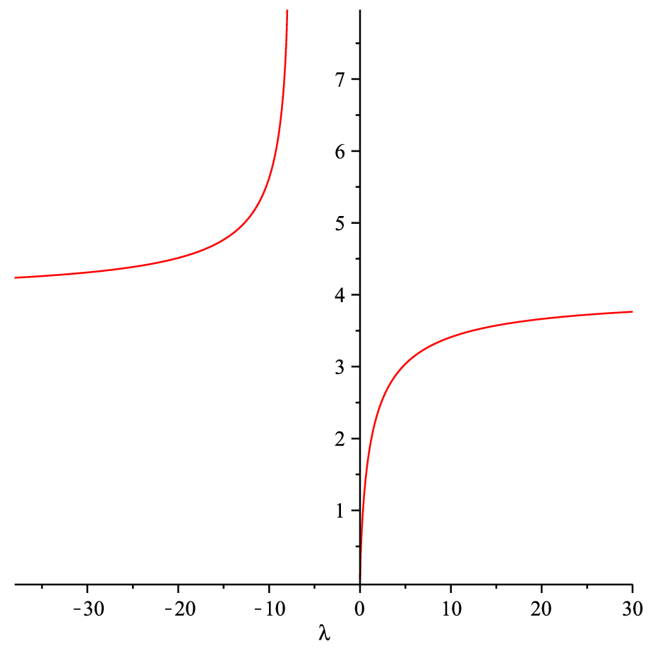
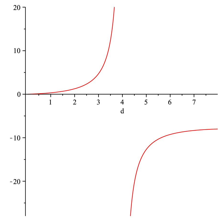
and where $u^{*}_{\lambda(d)}=G_{\lambda}/\|G_{\lambda}\|$ . Here $d(\lambda)$ is defined on $(-\infty,-8)\cup(0,\infty)$ , satisfies (3.6) and monotonically increases from $d(-\infty)=4$ to $d(-8)=8$ and then from $d(0)=0$ to $d(\infty)=4$ . The inverse function $\lambda(d)$ is defined on $d\in[0,8]\setminus\{0\}$ and satisfies

\lambda(8-d)=-8-\lambda(d).

Their graphs are shown in Fig. 3. Finally, $\mathbb{V}(4)=1$ and $u^{*}=\delta$ .

Proof.

We act as in Theorem 2.1, the essential difference being that we now do not have a formula for the inverse function $\lambda(d)$ , by means of which we construct the extremal element for each $d$ . Although $d(\lambda)$ is given explicitly, the monotonicity of it required for the existence of the inverse function is a rather general fact and can be verified as in [18, Theorem 2.1], where the continuous case was considered. ∎

We now find an explicit majorant $\mathbb{V}_{0}(d)$ for the implicitly defined solution $\mathbb{V}(d)$ . In view of the symmetry (3.4) it suffices to study the case $d\to 0$ only and then, by replacing $d\to d(8-d)/8$ we get the symmetric expansions valid for both singularities. We have the following expansions

		$\displaystyle d(\lambda)=(5\ln 2-\ln\lambda-1)\lambda+O_{\lambda\to 0}((\lambda\ln\lambda)^{2}),$		(3.19)
		$\displaystyle d(\lambda)=4-\frac{8}{\lambda}+O_{\lambda\to\infty}(1/\lambda^{2}).$		(3.19)

Truncating the first expansion and solving $d=(5\ln 2-\ln\lambda-1)\lambda$ , we have

\lambda=-\frac{d}{W_{-1}(-\frac{1}{32}ed)}

where $W_{-1}(z)$ is the $-1$ th branch of the Lambert function. Using the known asymptotic expansions for the Lambert function, we get the following expression for $\lambda(d)$

\lambda(d)=\frac{d}{5\ln 2-1-\ln(d)+\ln(5\ln(2)-1-\ln d)+O(\frac{\ln(-\ln d)}{\ln d})}.

(3.20)

Using

		$\displaystyle\frac{f^{2}(\lambda)}{g(\lambda)}=\frac{(\frac{5}{2}\ln 2-\frac{1}{2}\ln\lambda)^{2}}{\pi}\lambda+O_{\lambda\to 0}(\lambda^{2}(\ln\lambda)^{3}),$		(3.21)
		$\displaystyle\frac{f^{2}(\lambda)}{g(\lambda)}=1-\frac{4}{\lambda^{2}}+O_{\lambda\to\infty}\biggl(\frac{1}{\lambda^{3}}\biggr)$		(3.21)

and substituting (3.20) into the first expansion we get

\mathbb{V}(d)=\frac{1}{4\pi}d(-\ln d+\ln(1-\ln d)+\gamma+o_{d\to 0}(1))

where $\gamma=5\ln(2)+1<2\pi$ . This justifies our choice of the approximation to $\mathbb{V}(d)$ :

\mathbb{V}_{0}(d)=\frac{1}{4\pi}\frac{d(8-d)}{8}\left(\ln\frac{16}{d(8-d)}+\ln\biggl(1+\ln\frac{16}{d(8-d)}\biggr)+2\pi\right)

The constant $2\pi$ instead of $\gamma$ (and the numerator $16$ ) are chosen so that for $d=4$ we have $\mathbb{V}(4)=\mathbb{V}_{0}(4)=1$ .

The asymptotic expansion of $\mathbb{V}_{0}(d)$ at $d=0$ shows that $\mathbb{V}(d)<\mathbb{V}_{0}(d)$ for $0<d\leq d_{0}$ , where $d_{0}$ is sufficiently small.

Using the expansions at $\lambda=\infty$ in (3.19) and (3.21) we find that

\mathbb{V}(d)=1-\frac{(4-d)^{2}}{16}+O_{d\to 4}((4-d)^{3}).

Since

\mathbb{V}_{0}(d)=1-\left(1-\frac{1}{\pi}\right)\frac{(4-d)^{2}}{16}+O_{d\to 4}((4-d)^{3}),

it follows that $\mathbb{V}(d)\leq V_{0}(d)$ for $d\in[4-d_{1},4]$ for a small $d_{1}>0$ . Corresponding to $[d_{0},d_{1}]$ is the finite interval $[\lambda_{0},\lambda_{1}]$ on which computer calculations show that the inequality $\mathbb{V}(d)\leq V_{0}(d)$ still holds. This gives that

\mathbb{V}(d)\leq V_{0}(d)

for all $d\in[0,4]$ and hence, by symmetry, for $d\in[0,8]$ .

Thus, we have proved the following inequality.

Theorem 3.3.

For $u\in l_{2}(\mathbb{Z}^{2})$

u(0,0)^{2}\leq\frac{1}{4\pi}\frac{\|\nabla u\|^{2}}{\|u\|^{2}}\left(1-\frac{\|\nabla u\|^{2}}{8\|u\|^{2}}\right)\left(\ln\frac{16}{\frac{\|\nabla u\|^{2}}{\|u\|^{2}}\left(8-\frac{\|\nabla u\|^{2}}{\|u\|^{2}}\right)}+\right.\\ +\left.\ln\left(1+\ln\frac{16}{\frac{\|\nabla u\|^{2}}{\|u\|^{2}}\left(8-\frac{\|\nabla u\|^{2}}{\|u\|^{2}}\right)}\right)+2\pi\right),

(3.22)

where the constants in front of logarithms and $2\pi$ are sharp. The inequality saturates for $u=\delta$ , otherwise the inequality is strict.

4. 3D case

In the three-dimensional case the following result holds which is somewhat similar to the classical Sobolev inequality for the limiting exponent.

Theorem 4.1.

Let $u\in l^{2}(\mathbb{Z}^{3})$ . Then for any $\theta\in[0,1]$

u(0,0,0)^{2}\leq\mathrm{K}_{3}(\theta)\|u\|^{2\theta}\|\nabla u\|^{2(1-\theta)},

(4.1)

where $\mathrm{K}_{3}(\theta)<\infty$ for $\theta\in[0,1]$ , and its sharp value for $\theta\in(0,1)$ is given by

\mathrm{K}_{3}(\theta)=\frac{1}{2\pi^{2}}\frac{1}{\theta^{\theta}(1-\theta)^{1-\theta}}\max_{\lambda>0}\lambda^{\theta}\int_{0}^{\pi}\frac{K\left(\frac{1}{\frac{\lambda}{4}+1+\sin^{2}\frac{x}{2}}\right)}{\frac{\lambda}{4}+1+\sin^{2}\frac{x}{2}}dx,

(4.2)

and there exists a unique extremal element, which belongs to $l^{2}(\mathbb{Z}^{3})$ .

In the limiting case $\theta=0$ inequality (4.1) still holds:

u(0,0,0)^{2}\leq\mathrm{K}_{3}(0)\|\nabla u\|^{2},

(4.3)

where

	$\displaystyle\mathrm{K}_{3}(0)=\frac{1}{(2\pi)^{3}}\int_{\mathrm{T}^{3}}\frac{dx}{4(\sin^{2}\frac{x_{1}}{2}+\sin^{2}\frac{x_{2}}{2}+\sin^{2}\frac{x_{3}}{2})}=$		(4.4)
	$\displaystyle=\frac{1}{2\pi^{2}}\cdot\int_{0}^{\pi}\frac{K\left(\frac{1}{1+\sin^{2}\frac{x}{2}}\right)}{1+\sin^{2}\frac{x}{2}}dx=\frac{4.9887\dots}{2\pi^{2}}=0.2527\dots.$		(4.4)

The constant is sharp and there exists a unique extremal element, which does not lie in $l^{2}(\mathbb{Z}^{3})$ , but rather in $l^{\infty}_{0}(\mathbb{Z}^{3})$ , but whose gradient does belong to $l^{2}(\mathbb{Z}^{3})$ . Furthermore, as we already mentioned in §1, we have the closed form formula for $\mathrm{K}_{3}(0)$ (see [3])

\mathrm{K}_{3}(0)=\frac{\sqrt{6}}{24(2\pi)^{3}}\Gamma(\tfrac{1}{24})\Gamma(\tfrac{5}{24})\Gamma(\tfrac{7}{24})\Gamma(\tfrac{11}{24}).

Proof.

We have to find the fundamental solution $G_{\lambda}(k,l,m)$ of the equation

\mathbb{A}(\lambda)G_{\lambda}=(\mathrm{D}_{1}^{*}\mathrm{D}_{1}+\mathrm{D}_{2}^{*}\mathrm{D}_{2}+\mathrm{D}_{3}^{*}\mathrm{D}_{3}+\lambda)G_{\lambda}=\delta.

(4.5)

Similarly to the 1D and 2D cases we find that the function

\widehat{g}_{\lambda}(x,y,z):=\sum_{k,l,m=-\infty}^{\infty}G_{\lambda}(k,l,m)e^{ikx+ily+imz},

satisfies

\widehat{g}_{\lambda}(x,y,z)=\frac{\frac{1}{4}}{\frac{\lambda}{4}+\sin^{2}\frac{x}{2}+\sin^{2}\frac{y}{2}+\sin^{2}\frac{z}{2}}\,.

As before we have the inequality

u(0,0,0)^{2}\leq G_{\lambda}(0,0,0)(\|\nabla u\|^{2}+\lambda\|u\|^{2}),

(4.6)

which saturates for $u=\mathrm{const}\cdot G_{\lambda}$ .

For $\lambda>0$ as in the 1D and 2D cases we have $\widehat{g}_{\lambda}\in L_{2}(\mathbb{T}^{3})$ , and, hence, $G_{\lambda}\in l^{2}(\mathbb{Z}^{3})$ for $\lambda>0$ . In particular, using (3.10) we find

	$\displaystyle G_{\lambda}(0,0,0)=\frac{1}{8\pi^{3}}\int_{-\pi}^{\pi}\int_{-\pi}^{\pi}\int_{-\pi}^{\pi}\widehat{g}_{\lambda}(x,y,z)dxdydz=$		(4.7)
	$\displaystyle=\frac{1}{2\pi^{2}}\int_{0}^{\pi}\frac{K\left(\frac{1}{\frac{\lambda}{4}+1+\sin^{2}\frac{x}{2}}\right)}{\frac{\lambda}{4}+1+\sin^{2}\frac{x}{2}}dx.$		(4.7)

However, unlike the previous two cases, now $\widehat{g}_{\lambda}$ is integrable for all $\lambda\geq 0$ including $\lambda=0$ : $\widehat{g}_{\lambda}\in L_{1}(\mathbb{T}^{3})$ for $\lambda\geq 0$ . Therefore the Green’s function $G_{0}$ is well defined and belongs to $l^{\infty}_{0}(\mathbb{Z}^{3})$ . We point out, however, that since $\widehat{g}_{0}\notin L_{2}(\mathbb{T}^{3})$ , it follows that $G_{0}\notin l^{2}(\mathbb{Z}^{3})$ .

For $\lambda=0$ , the integrand has only a logarithmic singularity at $x=0$ and we obtain

\displaystyle G_{0}(0,0,0)=\frac{1}{2\pi^{2}}\int_{0}^{\pi}\frac{K\left(\frac{1}{1+\sin^{2}\frac{x}{2}}\right)}{1+\sin^{2}\frac{x}{2}}dx.

We now see that $f(\lambda):=G_{\lambda}(0,0,0)$ is continuous on $\lambda\in[0,\infty)$ and is of the order $1/\lambda$ at infinity. This gives that for $\theta\in(0,1)$ the function $\lambda^{\theta}f(\lambda)$ vanishes both at the origin and at infinity. Hence, it attains its maximum at a (generically) unique point $\lambda_{*}(\theta)$ , and the claim of the theorem concerning the case $\theta\in(0,1)$ follows in exactly the same way as in Theorem 2.2.

Setting $\lambda=0$ in (4.6) we obtain (4.3) with (4.4). It remains to verify that $\nabla G_{0}\in l^{2}(\mathbb{Z}^{3})$ . To see this we use notation (2.11) and Lemma 2.1. We obtain

	$\displaystyle\\|\nabla G_{\lambda}\\|^{2}=h(\lambda)=f(\lambda)+\lambda f^{\prime}(\lambda)=$
	$\displaystyle=\frac{1}{8\pi^{3}}\int_{-\pi}^{\pi}\int_{-\pi}^{\pi}\int_{-\pi}^{\pi}(\widehat{g}_{\lambda}(x,y,z)+\lambda\widehat{g}_{\lambda}(x,y,z)^{\prime}_{\lambda})dxdydz=$
	$\displaystyle=\frac{1}{8\pi^{3}}\int_{-\pi}^{\pi}\int_{-\pi}^{\pi}\int_{-\pi}^{\pi}\frac{\frac{1}{4}(\sin^{2}\frac{x}{2}+\sin^{2}\frac{y}{2}+\sin^{2}\frac{z}{2})}{(\frac{\lambda}{4}+\sin^{2}\frac{x}{2}+\sin^{2}\frac{y}{2}+\sin^{2}\frac{z}{2})^{2}}dxdydz.$

Since the integral on right-hand side is bounded for $\lambda=0$ we have $\|\nabla G_{0}\|^{2}<\infty$ . Finally, $G_{\lambda}$ has strictly positive elements for $\lambda\geq 0$ , since we have as before the maximum principle. In the case when $\lambda=0$ we use, in addition, the fact that $G_{0}\in l^{\infty}_{0}$ . The proof is complete. ∎

The graph of $\mathrm{K}_{3}(\theta)$ is shown in Fig. 4.

Remark 4.1.

Higher dimensional cases are treated similarly, in particular, for $d\geq 3$ and $\theta=0$

u(0)^{2}\leq\mathrm{K}_{d}(0)\|\nabla u\|^{2},\ \mathrm{K}_{d}(0)=\frac{1}{(2\pi)^{d}}\int_{\mathrm{T}^{d}}\frac{dx}{4(\sin^{2}\frac{x_{1}}{2}+\dots+\sin^{2}\frac{x_{d}}{2})}\,.

(4.8)

In §6 we give an independent elementary proof of this inequality.

5. Higher order difference operators

The method developed above admits a straight forward generalization to higher order difference operators. We consider the second-order operator in the one dimensional case:

u(0)^{2}\leq\mathrm{K}_{1,2}(\theta)\|u\|^{2\theta}\|\Delta u\|^{2(1-\theta)},

(5.1)

where

-\Delta u(n):=\mathrm{D}^{*}\mathrm{D}u(n)=-\bigl(u(n+1)-2u(n)+u(n-1)\bigr).

Accordingly, the operator $\mathbb{A}(\lambda)$ is

\mathbb{A}(\lambda)=\left\{\begin{array}[]{ll}\phantom{-}\Delta^{2}+\lambda,&\hbox{for $\lambda>0$;}\\ -\Delta^{2}-\lambda,&\hbox{for $\lambda<-16$.}\end{array}\right.

(5.2)

Here

\Delta^{2}u(n)=u(n+2)-4u(n+1)+6u(n)-4u(n-1)+u(n-2).

As before, we have to find the Green’s function $G_{\lambda}$ solving $\mathbb{A}(\lambda)G_{\lambda}=\delta$ . Furthermore, for finding $\mathrm{K}_{1,2}(\theta)$ it suffices to solve this equation for $\lambda>0$ . Setting

\widehat{g}_{\lambda}(x):=\sum_{n=-\infty}^{\infty}G_{\lambda}(n)e^{inx},

and arguing as in Lemma 2.2 we get from (5.2)

	$\displaystyle 1=\widehat{g}_{\lambda}(x)(\lambda+e^{-i2x}-4e^{-ix}+6-4e^{ix}+e^{i2x})=$		(5.3)
	$\displaystyle=\widehat{g}_{\lambda}(x)\bigl(\lambda+(e^{ix/2}-e^{-ix/2})^{4}\bigr)=\widehat{g}_{\lambda}(x)\left(\lambda+16\sin^{4}\frac{x}{2}\right),$		(5.3)

so that

G_{\lambda}(0)=\frac{1}{2\pi}\int_{-\pi}^{\pi}\frac{dx}{\lambda+16\sin^{4}\frac{x}{2}}=\frac{\sqrt{2}}{2}\frac{1}{\lambda^{3/4}}\sqrt{\frac{\sqrt{\lambda+16}+\sqrt{\lambda}}{\lambda+16}}\,.

(5.4)

Now a word for word repetition of the argument in Theorem 2.2 gives that

\mathrm{K}_{1,2}(\theta)=\frac{1}{\theta^{\theta}(1-\theta)^{1-\theta}}\cdot\sup_{\lambda>0}\lambda^{\theta}G_{\lambda}(0).

Therefore we see from (5.4) that $\mathrm{K}_{1,2}(\theta)<\infty$ if and only if

\frac{3}{4}\leq\theta\leq 1.

For example, for $\theta=3/4$ supremum is the maximum attained at $\lambda_{*}(3/4)=16/3$ , giving

\mathrm{K}_{1,2}(3/4)=\frac{4}{3^{3/4}}\cdot\lambda^{3/4}G_{\lambda}(0)|_{\lambda_{*}(3/4)=\frac{16}{3}}=\frac{\sqrt{2}}{2}.

We only mention that in the general case

	$\displaystyle\lambda_{*}(\theta)=\mathrm{argmax}_{\lambda>0}\,\lambda^{\theta-3/4}\sqrt{\frac{\sqrt{\lambda+16}+\sqrt{\lambda}}{\lambda+16}}=$		(5.5)
	$\displaystyle=\frac{64\theta-32\theta^{2}-29+\sqrt{32\theta-23}}{2\theta^{2}-5\theta+3},$		(5.5)

however, the corresponding substitution produces a long (but explicit) formula for $\mathrm{K}_{1,2}(\theta)$ , and instead we present in Fig.5 the graph of the sharp constant $\mathrm{K}_{1,2}(\theta)$ , where $\mathrm{K}_{1,2}(3/4)=\sqrt{2}/2$ and $\mathrm{K}_{1,2}(1)=1$ .

Finally, it is possible to find $G_{\lambda}(n)$ explicitly. In fact, the free recurrence relation $\Delta^{2}G_{\lambda}+\lambda G_{\lambda}=0$ has the characteristic equation

q^{2}-4q+(6+\lambda)-4q^{-1}+q^{-2}=0,

or $(q^{1/2}-q^{-1/2})^{4}=-\lambda$ , which decomposes into two quadratic equations

q+\frac{1}{q}-2=i\sqrt{\lambda}\quad\text{and}\quad q+\frac{1}{q}-2=-i\sqrt{\lambda},

with four roots $q_{1},q_{2},q_{3},q_{4}$ , where $q_{2}=1/q_{1}$ , $q_{3}=\bar{q}_{2}$ , $q_{4}=\bar{q}_{1}$ , where

q_{1}=q(\lambda)=1-\frac{\lambda^{1/4}\sqrt{\sqrt{\lambda+16}-\sqrt{\lambda}}}{2\sqrt{2}}+i\left(\frac{\sqrt{\lambda}}{2}-\frac{\lambda^{1/4}\sqrt{\sqrt{\lambda+16}+\sqrt{\lambda}}}{2\sqrt{2}}\right).

(5.6)

Since $|q(\lambda)|<1$ for $\lambda>0$ , it follows that any symmetric $l_{2}$ -solution of (5.2) is of the form $a(\lambda)q(\lambda)^{|n|}+b(\lambda)\bar{q}(\lambda)^{|n|}$ , and since, in addition $G_{\lambda}(n)$ is real, we have

G_{\lambda}(n)=a(\lambda)q(\lambda)^{|n|}+\bar{a}(\lambda)\bar{q}(\lambda)^{|n|}.

Setting $n=0$ and $n=1$ we obtain a linear system for $a(\lambda)$

		$\displaystyle G_{\lambda}(0)=2\mathop{\mathrm{}}{Re}a(\lambda)$
		$\displaystyle G_{\lambda}(1)=a(\lambda)q(\lambda)+\bar{a}(\lambda)\bar{q}(\lambda),$

where $G_{\lambda}(0)$ is given in (5.4) and

G_{\lambda}(1)=\frac{1}{\pi}\int_{0}^{\pi}\frac{\cos x\,dx}{\lambda+16\sin^{4}\frac{x}{2}}=\frac{\sqrt{2}}{2}\frac{1}{\lambda^{3/4}}\frac{\sqrt{\lambda+16}-\sqrt{\lambda}}{\sqrt{\sqrt{\lambda+16}+\sqrt{\lambda}}\,\sqrt{\lambda+16}}\,.

Solving this system we find $a(\lambda)$ :

a(\lambda)=\frac{\sqrt{2}}{4}\frac{1}{{\lambda^{3/4}}\sqrt{\lambda+16}\sqrt{\sqrt{\lambda+16}+\sqrt{\lambda}}}\left(\sqrt{\lambda+16}+\sqrt{\lambda}+4i\right),

and, consequently, the formula for $G_{\lambda}(n)$ with $\lambda>0$ :

\displaystyle G_{\lambda}(n)=\frac{1}{\pi}\int_{0}^{\pi}\frac{\cos nx\,dx}{\lambda+16\sin^{4}\frac{x}{2}}=\frac{\mathop{\mathrm{}}{Re}\left[\bigl(\sqrt{\lambda+16}+\sqrt{\lambda}+4i\bigr)\cdot q(\lambda)^{|n|}\right]}{\sqrt{2}\,{\lambda^{3/4}}\sqrt{\lambda+16}\sqrt{\sqrt{\lambda+16}+\sqrt{\lambda}}},

(5.7)

where $q(\lambda)$ is given in (5.6).

Thus, we obtain the following result.

Theorem 5.1.

Inequality (5.1) holds for $\theta\in[3/4,1]$ . In particular, in the limiting case $\theta=3/4$

u(0)^{2}\leq\frac{\sqrt{2}}{2}\,\|u\|^{3/2}\|\Delta u\|^{1/2}.

(5.8)

In the general case,

\mathrm{K}_{1,2}(\theta)=\frac{1}{\theta^{\theta}(1-\theta)^{1-\theta}}\cdot\lambda_{*}(\theta)^{\theta}G_{\lambda_{*}(\theta)}(0),

where $\lambda_{*}(\theta)$ is given in (5.5) and $G_{\lambda}(0)$ in (5.4) (see also (5.7)). For $\theta\in[3/4,1)$ the unique extremal is $u_{\lambda_{*}(\theta)}=G_{\lambda_{*}(\theta)}$ . For $\theta=1$ , $\lambda_{*}(1)=\infty$ and $u_{*}=\delta$ .

Remark 5.1.

It is not difficult to find the function $\mathbb{V}(d)$ , that is, the solution of the maximization problem

\mathbb{V}(d):=\sup\bigl\{u(0)^{2}:\ u\in l^{2}(\mathbb{Z}),\ \|u\|^{2}=1,\ \|\Delta u\|^{2}=d\bigr\},

(5.9)

where $d\in[0,16]$ . For this purpose we also need the expression for the Green’s function $G_{\lambda}(0)$ in the region $\lambda\leq-16$ , which is as follows

G_{\lambda}(0)=-\frac{1}{2\pi}\int_{-\pi}^{\pi}\frac{dx}{\lambda+16\sin^{4}\frac{x}{2}}=\frac{1}{2(-\lambda)^{3/4}}{\frac{\sqrt{\sqrt{-\lambda}+4}+\sqrt{\sqrt{-\lambda}-4}}{\sqrt{-\lambda-16}}}\,.

(5.10)

Using (5.4), (5.10) we can write down a parametric representation of $\mathbb{V}(d)$ as in Theorem 3.2, but instead we merely show its graph in Fig.7.

This time we do not have the maximum principle, and the Green’s function $G_{\lambda}(n)$ is not positive for all $n$ , but is rather oscillating with exponentially decaying amplitude, see Fig. 6. Nor do we have the symmetry $\mathbb{V}(d)=\mathbb{V}(16-d)$ in Fig. 7 that we have seen in the first-order inequalities in the one- and two-dimensional cases, see (2.8) and (3.4). The maximum is attained at $d=6$ corresponding to $u=\delta$ . The component $\lambda\in(0,\infty)$ of the resolvent set corresponds to $d\in(0,6)$ and $\lambda\in(-\infty,-16)$ corresponds to $d\in(6,16)$ .

It is worth to compare the results so obtained in the discrete case with the corresponding interpolation inequalities for Sobolev spaces in the continuous case. It is well known that the interpolation inequality on the whole line $\mathbb{R}$

\|f\|^{2}_{L_{\infty}}\leq\mathrm{C}_{1,n}(\theta)\|f\|^{2\theta}\|f^{(n)}\|^{2(1-\theta)},

(5.11)

where $f\in H^{n}(\mathbb{R})$ , holds only for $\theta=1-\tfrac{1}{2n}$ . The sharp constant was found in [17]:

\mathrm{C}_{1,n}(\theta)=\frac{1}{\theta^{\theta}(1-\theta)^{1-\theta}}\frac{1}{\pi}\int_{0}^{\infty}\frac{dx}{1+x^{2n}}=\frac{1}{\theta^{\theta}(1-\theta)^{1-\theta}}\frac{1}{2n}\frac{1}{\sin\frac{\pi}{2n}}\,.

(5.12)

Thus, for first-order inequalities both in the discrete and continuous cases the constants are equal to $1$ , while for the second-order inequalities we see from (5.8) and (5.12) that

\mathrm{C}_{1,2}(3/4)=\left(\frac{4}{27}\right)^{1/4}<\frac{\sqrt{2}}{2}=\mathrm{K}_{1,2}(3/4).

The next theorem states that for higher order inequalities the constants in the discrete case are always strictly greater than those in the continuous case.

Theorem 5.2.

Let $n\geq 1$ and let $u\in l^{2}(\mathbb{Z})$ . The inequality

u(0)^{2}\leq\mathrm{K}_{1,n}(\theta)\|u\|^{2\theta}\|\mathcal{D}^{n}u\|^{2(1-\theta)},

(5.13)

where

\mathcal{D}^{n}:=\left\{\begin{array}[]{ll}\Delta^{n/2},&\hbox{for $n$ even,}\\ \nabla\Delta^{(n-1)/2},&\hbox{for $n$ odd,}\end{array}\right.

(5.14)

holds for $\theta\in[1-1/(2n),1]$ and

\mathrm{K}_{1,n}(\theta)=\frac{1}{\theta^{\theta}(1-\theta)^{1-\theta}}\frac{1}{\pi}\sup_{\lambda>0}\lambda^{\theta}\int_{0}^{\pi}\frac{dx}{\lambda+2^{2n}\sin^{2n}\frac{x}{2}}\,.

(5.15)

For all $\theta\in[1-1/(2n),1]$ supremum is the maximum. If $n\geq 2$ , then for $\theta=\theta_{*}:=1-1/(2n)$ the constants in the continuous and discrete inequalities satisfy

\mathrm{C}_{1,n}(\theta_{*})<\mathrm{K}_{1,n}(\theta_{*}).

(5.16)

Proof.

Following the scheme developed above we look for the solution of the equation

(-1)^{n}\Delta^{n}G_{\lambda}+\lambda G_{\lambda}=\delta,

and as in (5.3) find that

G_{\lambda}(0)=\frac{1}{\pi}\int_{0}^{\pi}\frac{dx}{\lambda+2^{2n}\sin^{2n}\frac{x}{2}},

which proves (5.15) (whenever the supremum is finite). Using $\sin^{2}\frac{x}{2}=\tan^{2}\frac{x}{2}/(1+\tan^{2}\frac{x}{2})$ and changing the variable $\tan\frac{x}{2}=\sqrt{\mu}t$ , where $\mu=\lambda^{1/n}$ we have

\lambda^{\theta_{*}}\int_{0}^{\pi}\frac{dx}{\lambda+2^{2n}\sin^{2n}\frac{x}{2}}=\int_{0}^{\infty}\frac{2dt}{(1+\mu t^{2})(1+\frac{2^{2n}t^{2n}}{(1+\mu t^{2})^{n}})}=:S(\mu).

Clearly $S(\infty)=0$ , and we have to study $S(\mu)$ as $\mu\to 0$ . The integral converges uniformly for $\mu\in[0,1]$ , since the denominator is greater then $1$ for $t\in[0,1]$ and is greater then $1+c(n)t^{2}$ for $t\geq 1$ observing that $t^{2n}/(1+\mu t^{2})^{n-1}\geq c_{1}(n)t^{2}$ uniformly for $\mu\in[0,1]$ . Therefore

\lim_{\mu\to 0}S(\mu)=S(0)=\int_{0}^{\infty}\frac{2dt}{1+2^{2n}t^{2n}}=\int_{0}^{\infty}\frac{dx}{1+x^{2n}}\,,

which proves, in the first place, that the right-hand side in (5.15) is finite if and only if $\theta\in[\theta_{*},1]$ and, secondly, that non-strict inequality (5.16) holds. Finally, for $n\geq 2$ we have strict inequality since

S^{\prime}_{\mu}(0)=2\int_{0}^{\infty}\left[\frac{n2^{2n}t^{2n+2}}{(1+2^{2n}t^{2n})^{2}}-\frac{t^{2}}{1+2^{2n}t^{2n}}\right]dt=\frac{1}{16n}\frac{\pi}{\sin\frac{3\pi}{2n}}>0.

For $n=1$ we have $\lambda=\mu$ , $S^{\prime}_{\mu}(0)<0$ and

S(\mu)=\frac{\pi}{\sqrt{\mu+4}}

is strictly decreasing not only at $\mu=0$ but for all $\mu\geq 0$ , the fact that we have already seen in (2.24). ∎

Remark 5.2.

Inequality (5.13) holds for $\theta\in[1-1/(2n),1]$ , that is, when the weight of the stronger norm, which is the $l_{2}$ -norm, increases. Accordingly, inequality (5.11) for periodic functions with mean value zero holds for $\theta$ in the complementary interval $\theta\in[0,1-1/(2n)]$ , when the weight of the stronger norm, which is the $L_{2}$ -norm of the $n$ -th derivative, increases:

\|f\|^{2}_{L_{\infty}}\leq\mathrm{C}_{1,n}^{\mathrm{per}}(\theta)\|f\|^{2\theta}\|f^{(n)}\|^{2(1-\theta)},\qquad\theta\in[0,1-\tfrac{1}{2n}],

(5.17)

where

f\in H^{n}_{\mathrm{per}}(\mathbb{S}^{1}),\qquad\int_{0}^{2\pi}f(x)dx=0.

A general method for finding sharp constants in interpolation inequalities of $L_{\infty}$ - $L_{2}$ - $L_{2}$ -type was developed in [11], [1], [18], which was also used in the discrete case in the present paper. For example, for $n=1$

\mathrm{C}_{1,1}^{\mathrm{per}}(\theta)=\frac{1}{\theta^{\theta}(1-\theta)^{1-\theta}}\sup_{\lambda\geq 0}\lambda^{\theta}G(\lambda),\qquad\theta\in[0,1/2],

(5.18)

where $G_{\lambda}(x,\xi)=\frac{1}{2\pi}\sum_{x\in\mathbb{Z}\setminus\{0\}}\frac{e^{ik(x-\xi)}}{k^{2}+\lambda}$ is the Green’s function of the equation

-G_{\lambda}(x,\xi)^{\prime\prime}+\lambda G_{\lambda}(x,\xi)=\delta(x-\xi),\quad x,\xi\in[0,2\pi]^{\mathrm{per}},

and

G(\lambda):=G_{\lambda}(\xi,\xi)=\frac{1}{\pi}\sum_{k=1}^{\infty}\frac{1}{k^{2}+\lambda}=\frac{1}{2\pi}\frac{\pi\sqrt{\lambda}\coth(\pi\sqrt{\lambda})-1}{\lambda}.

For the limiting $\theta=\theta_{*}$ =1/2 the constant is the same as on $\mathbb{R}$ : $\mathrm{C}_{1,1}^{\mathrm{per}}(\theta_{*})=\mathrm{C}_{1,1}(\theta_{*})=1$ . The graph of $\mathrm{C}_{1,1}^{\mathrm{per}}(\theta)$ on the interval $\theta\in[0,1/2]$ is shown in Fig.1 on the left. Observe that $\mathrm{C}_{1,1}(0)=\pi/6$ .

6. Applications

Discrete and integral Carlson inequalities

We now discuss applications of the inequalities for the discrete operators, and our first group of results concerns Carlson inequalities. The original Carlson inequality [5] is as follows:

\left(\sum_{k=1}^{\infty}a_{k}\right)^{2}\leq\pi\left(\sum_{k=1}^{\infty}a_{k}^{2}\right)^{1/2}\left(\sum_{k=1}^{\infty}k^{2}a_{k}^{2}\right)^{1/2},

(6.1)

where the constant $\pi$ is sharp and cannot be attained at a non identically zero sequence $\{a_{k}\}_{k=1}^{\infty}$ . This inequality has attracted a lot of interest and has been a source of generalizations and improvements (see, for example, [10], [12] and the references therein, and also [18] for the most recent strengthening of (6.1)). Inequality (6.1) has an integral analog (with the same sharp constant)

\left(\int_{0}^{\infty}g(t)dt\right)^{2}\leq\pi\left(\int_{0}^{\infty}g(t)^{2}dt\right)^{1/2}\left(\int_{0}^{\infty}t^{2}g(t)^{2}dt\right)^{1/2}.

(6.2)

As was first observed in [9], inequality (6.1) is equivalent to the inequality

\|f\|_{\infty}^{2}\leq 1\cdot\|f\|\|f^{\prime}\|,

(6.3)

for periodic functions $f\in H^{1}_{\mathrm{per}}(0,2\pi)$ , $\int_{0}^{2\pi}f(x)dx=0$ , by setting for a sequence $\{a_{k}\}_{k=1}^{\infty}$

f(x)=\sum_{k=-\infty}^{\infty}a_{|k|}e^{ikx},\qquad a_{0}=0.

Accordingly, inequality (6.3) for $f\in H^{1}(\mathbb{R})$ is equivalent (as was first probably observed in [15]) to (6.2) by setting $g=\mathcal{F}f$ and further restricting $g$ (and $f$ ) to even functions. Furthermore, the unique (up to scaling) extremal function $f_{*}(x)=e^{-|x|}$ in (6.3) on the whole axis produces the extremal function $g_{*}(t)=1/(1+t^{2})$ in (6.2).

In the similar way, discrete inequalities have equivalent integral analogs. Let $\mathscr{F}$ be the discrete Fourier transform $\mathscr{F}:\{a(n)\}\to\widehat{a}(x)$ , where

\widehat{a}(x)=\sum_{n\in\mathbb{Z}^{d}}a(n)e^{inx},\qquad a(n)=(2\pi)^{-d}\int_{\mathbb{T}^{d}}\widehat{a}(x)e^{-inx}dx.

Then for $e_{j}=(0,\dots,0,1,0,\dots,0)$ with $1$ on the $j$ th place

	$\displaystyle\mathrm{D}_{j}a(n)=a(n+e_{j})-a(n)=(2\pi)^{-d}\int_{\mathbb{T}^{d}}\widehat{a}(x)(e^{-i(n+e_{j})x}-e^{-inx})dx=$
	$\displaystyle=(2\pi)^{-d}\int_{\mathbb{T}^{d}}\widehat{a}(x)e^{-ix/2}(-2i)\sin\tfrac{x_{j}}{2}\,e^{-inx}dx.$

Therefore

\|\mathrm{D}_{j}a\|^{2}=(2\pi)^{-d}\int_{\mathbb{T}^{d}}|\widehat{a}(x)|^{2}4\sin^{2}\tfrac{x_{j}}{2}\,dx.

(6.4)

and, finally,

\|a\|^{2}=(2\pi)^{-d}\|\widehat{a}\|^{2},\ \|\nabla a\|^{2}=(2\pi)^{-d}\int_{\mathbb{T}^{d}}|\widehat{a}(x)|^{2}4\sum_{j=1}^{d}\nolimits\sin^{2}\tfrac{x_{j}}{2}\,dx.

(6.5)

Thus, we have proved the following result.

Theorem 6.1.

Let $1/2<\theta\leq 1$ . The inequality

u(0)^{2}\leq\mathrm{K}_{1}(\theta)\|u\|^{2\theta}\|\mathrm{D}u\|^{2(1-\theta)},\qquad u\in l_{2}(\mathbb{Z})

established in Theorem 2.2 is equivalent to the inequality

\left(\int_{0}^{2\pi}g(x)dx\right)^{2}\leq 2\pi\mathrm{K}_{1}(\theta)\left(\int_{0}^{2\pi}g(x)^{2}dx\right)^{\theta}\left(\int_{0}^{2\pi}4\sin^{2}\tfrac{x}{2}\,g(x)^{2}dx\right)^{1-\theta},

(6.6)

for $g\in L_{2}(0,2\pi)$ . Here $\mathrm{K}_{1}(\theta)=\frac{1}{2}\left(2/\theta\right)^{\theta}(2\theta-1)^{\theta-1/2}$ (see (2.28)). In the limiting case inequality (2.27) is equivalent to

		$\displaystyle\left(\int_{0}^{2\pi}g(x)dx\right)^{2}\leq$		(6.7)
	$\displaystyle\pi\sqrt{4-\frac{\int_{0}^{2\pi}4\sin^{2}\tfrac{x}{2}\,g(x)^{2}dx}{\int_{0}^{2\pi}g(x)^{2}dx}}$	$\displaystyle\left(\int_{0}^{2\pi}g(x)^{2}dx\right)^{1/2}\left(\int_{0}^{2\pi}4\sin^{2}\tfrac{x}{2}\,g(x)^{2}dx\right)^{1/2}$		(6.7)

Proof.

The proof follows from Theorem 2.2 and (6.4). We also point out that for $\theta\in(1/2,1)$ inequality (6.6) saturates for

{g}_{\lambda_{*}}(x)=\frac{1}{\lambda_{*}+4\sin^{2}\frac{x}{2}}\,,\qquad\lambda_{*}=\lambda_{*}(\theta)=\frac{4\theta-2}{1-\theta}\,.

for $\theta=1/2$ no extremals exist and maximizing sequence is obtained by letting $\lambda_{*}\to 0$ ; finally for $\theta=1$ , (6.6) saturates at constants.

For each $d$ , $0<d<4$ and $\lambda(d)=\frac{2d}{{2-d}}$ inequality (6.7) saturates at

{g}_{\lambda(d)}(x)=\frac{1}{\lambda(d)+4\sin^{2}\frac{x}{2}}\,,\ \text{with}\ \frac{\int_{0}^{2\pi}4\sin^{2}\tfrac{x}{2}\,g_{\lambda(d)}(x)^{2}dx}{\int_{0}^{2\pi}g_{\lambda(d)}(x)^{2}dx}=d.

For $d=2$ , ${g}=\mathrm{const}$ . ∎

Remark 6.1.

Corresponding to (5.8) is the integral inequality

\left(\int_{0}^{2\pi}g(x)dx\right)^{2}\leq\pi\sqrt{2}\left(\int_{0}^{2\pi}g(x)^{2}dx\right)^{3/4}\left(\int_{0}^{2\pi}16\sin^{4}\tfrac{x}{2}\,g(x)^{2}dx\right)^{1/4},

(6.8)

which turns into equality for

g_{*}(x)=\frac{1}{\frac{16}{3}+16\sin^{4}\frac{x}{2}}\,.

Remark 6.2.

The integral analog of the two dimensional discrete inequality is

		$\displaystyle\left(\int_{\mathbb{T}^{2}}g(x,y)dxdy\right)^{2}\leq$		(6.9)
	$\displaystyle(2\pi)^{2}\mathrm{K}_{2}(\theta)$	$\displaystyle\left(\int_{\mathbb{T}^{2}}g(x,y)^{2}dxdy\right)^{\theta}\left(\int_{\mathbb{T}^{2}}4(\sin^{2}\tfrac{x}{2}+\sin^{2}\tfrac{y}{2})\,g(x,y)^{2}dxdy\right)^{1-\theta},$		(6.9)

where $\theta\in(0,1]$ , and $\mathrm{K}_{2}(\theta)$ is defined in (3.11).

Remark 6.3.

In the $d$ -dimensional case, $d\geq 3$ , for the exponent $\theta=0$ the Parceval’s identities (6.5) provide an independent elementary proof of (4.8). In fact, setting $g_{0}(x)=4\sum_{j=1}^{d}\nolimits\sin^{2}\tfrac{x_{j}}{2}$ we have

	$\displaystyle(2\pi)^{2d}\|a(0)\|^{2}=\left\|\int_{\mathbb{T}^{d}}\widehat{a}(x)dx\right\|^{2}\leq$		(6.10)
	$\displaystyle\leq\left(\int_{\mathbb{T}^{d}}\|\widehat{a}(x)\|g_{0}(x)^{1/2}g_{0}(x)^{-1/2}dx\right)^{2}\leq$
	$\displaystyle\leq\int_{\mathbb{T}^{d}}\|\widehat{a}(x)\|^{2}g_{0}(x)dx\int_{\mathbb{T}^{d}}g_{0}(x)^{-1}dx=(2\pi)^{2d}\mathrm{K}_{d}(0)\\|\nabla a\\|^{2},$

which proves (4.8).

This approach can be generalized to the $l^{p}$ -case for the proof of the discrete Sobolev type inequality in the non-limiting case (1.12). Here in addition to the Parseval’s identity we also use the Hausdorff-Young inequality (see, for instance, [2]):

\|\widehat{a}\|_{L_{p}(\mathbb{T}^{d})}\leq(2\pi)^{d/p}\|a\|_{l^{p^{\prime}}(\mathbb{Z}^{d})},

(6.11)

where $p\geq 2$ and $p^{\prime}=p/(p-1)$ .

In fact, we have $\|\mathscr{F}\|_{l^{2}\to L_{2}}=(2\pi)^{d/2}$ and $\|\mathscr{F}\|_{l^{1}\to L_{\infty}}=1$ and by the Riesz–Thorin interpolation theorem

\|\mathscr{F}\|_{l^{p^{\prime}}\to L_{p}}\leq(2\pi)^{d\theta/2}=(2\pi)^{d/p},

where $\frac{1}{p^{\prime}}=\frac{\theta}{2}+\frac{1-\theta}{1}$ , $\frac{1}{p}=\frac{\theta}{2}+\frac{1-\theta}{\infty}$ . We also observe that (6.11) becomes an equality for $\widehat{a}(x)=1$ and $a=\delta$ .

Setting $q=2p$ in (1.12), $v(n):=\overline{u(n)^{p}}u(n)^{p-1}$ , and using the auxiliary inequality (6.12), (6.13) below, we obtain

	$\displaystyle\\|u\\|_{l^{2p}}^{2p}=\sum_{n\in\mathbb{Z}^{d}}v(n)u(n)=\sum_{n\in\mathbb{Z}^{d}}(\mathrm{D}^{*}\mathrm{D}\Delta^{-1}v(n))u(n)=$
	$\displaystyle=\sum_{n\in\mathbb{Z}^{d}}\mathrm{D}\Delta^{-1}v(n)\mathrm{D}u(n)\leq\left(\sum_{n\in\mathbb{Z}^{d}}\|\mathrm{D}\Delta^{-1}v(n)\|^{2}\right)^{1/2}\\|\mathrm{D}u\\|\leq$
	$\displaystyle\leq\left(\frac{1}{4}(2\pi)^{d/p^{\prime}}I_{p^{\prime},d}\right)^{1/2}\\|v\\|_{l^{(2p)^{\prime}}}\\|\mathrm{D}u\\|=\left(\frac{1}{4}(2\pi)^{d/p^{\prime}}I_{p^{\prime},d}\right)^{1/2}\\|u\\|_{l^{2p}}^{2p-1}\\|\mathrm{D}u\\|.$

It remains to prove (6.12). By Hölder’s inequality and (6.11) we have

	$\displaystyle\sum_{n\in\mathbb{Z}^{d}}\|\mathrm{D}\Delta^{-1}v(n)\|^{2}=\frac{(2\pi)^{d}}{4}\int_{\mathrm{T}^{d}}\frac{\|\widehat{v}(x)\|^{2}dx}{\sum_{j=1}^{d}\nolimits\sin^{2}\tfrac{x_{j}}{2}}\leq$		(6.12)
	$\displaystyle\leq\frac{(2\pi)^{d}}{4}I_{p^{\prime},d}\left(\int_{\mathrm{T}^{d}}{\|\widehat{v}(x)\|^{2p}dx}\right)^{1/p}\leq$
	$\displaystyle\leq\frac{(2\pi)^{d}}{4}I_{p^{\prime},d}(2\pi)^{d/p}\\|v\\|_{l^{(2p)^{\prime}}}^{2}=\frac{1}{4}(2\pi)^{d(p+1)/p}I_{p^{\prime},d}\\|v\\|_{l^{(2p)^{\prime}}}^{2}$

where

I_{p^{\prime},d}=\left(\int_{\mathrm{T}^{d}}\frac{dx}{(\sum_{j=1}^{d}\nolimits\sin^{2}\tfrac{x_{j}}{2})^{p^{\prime}}}\right)^{1/p^{\prime}}\!<\infty\ \text{for}\ p^{\prime}<d/2\Leftrightarrow p>d/(d-2).

(6.13)

Thus we obtain the following result.

Theorem 6.2.

Let $d\geq 3$ and $2p>2d/(d-2)$ . Then

\|u\|^{2}_{l^{2p}(\mathbb{Z})^{d}}=\left(\sum_{n\in\mathrm{Z}^{d}}|u(n)|^{2p}\right)^{1/p}\leq\frac{1}{4}(2\pi)^{d(p+1)/p}I_{p^{\prime},d}\|\mathrm{D}u\|^{2},

where $I_{p^{\prime},d}$ is defined in (6.13).

Remark 6.4.

We do not claim that the constant here is sharp. Moreover, it blows up for $2p=2d/(d-2)$ , while it can be shown that the inequality still holds. However, the constant is sharp in the opposite limit $p=\infty$ , see (4.8).

Spectral inequalities for discrete operators

Interpolation inequalities characterizing imbeddings of Sobolev spaces into the space of bounded continuous functions have important applications in spectral theory. The original fruitful idea in [7] has been generalized in [6] to give best-known estimates for the Lieb–Thirring constants in estimates for the negative trace of Schrödinger operators.

In this section we apply our sharp interpolation inequalities with the method of [7] for estimates of the negative trace of the discrete operators [16].

We write the inequalities obtained above in the unform way

\sup_{k\in\mathbb{Z}^{d}}u(k)^{2}\leq\mathrm{K}(\theta)\|u\|^{2\theta}\|\mathcal{D}^{n}u\|^{2(1-\theta)},

(6.14)

where $\mathcal{D}^{n}$ is as in (5.14) and $\theta$ belongs to a certain subinterval of $[0,1]$ uniquely defined in the corresponding theorem:

\theta\in\left\{\begin{array}[]{ll}$[1-1/(2n),1]$,&\hbox{$d=1$, $n\geq 1$;}\\ $(0,\,1]$,&\hbox{$d=2$, $n=1$;}\\ $[0,\,1]$,&\hbox{$d\geq 3$, $n=1$.}\end{array}\right.

(6.15)

Theorem 6.3.

Let $\{u^{(j)}\}_{j=1}^{N}\in l^{2}(\mathbb{Z}^{d})$ be a family of $N$ sequences that are orthonormal with respect to the natural scalar product in $l^{2}(\mathbb{Z}^{d})$ . We set

\rho(k):=\sum_{j=1}^{N}u^{(j)}(k)^{2},\qquad k\in\mathbb{Z}^{d}.

(6.16)

Then for $\theta$ as in (6.15) and $\theta<1$

\|\rho\|_{l^{\frac{2-\theta}{1-\theta}}}^{\frac{2-\theta}{1-\theta}}=\sum_{k\in\mathbb{Z}^{d}}\rho(k)^{\frac{2-\theta}{1-\theta}}\leq\mathrm{K}(\theta)^{\frac{1}{1-\theta}}\sum_{j=1}^{N}\|\mathcal{D}^{n}u^{(j)}\|^{2}.

(6.17)

Proof.

For arbitrary $\xi_{1},\dots,\xi_{N}\in\mathbb{R}$ we construct a sequence $f\in l^{2}(\mathbb{Z}^{d})$

f(k):=\sum_{j=1}^{N}\xi_{j}u^{(j)}(k),\qquad k\in\mathbb{Z}^{d}.

Applying (6.14) and using orthonormality we obtain for a fixed $k$

f(k)^{2}\leq\mathrm{K}(\theta)\left(\sum_{j=1}^{N}\xi_{j}^{2}\right)^{\theta}\left(\sum_{i,j=1}^{N}\xi_{i}\xi_{j}\bigl(\mathcal{D}^{n}u^{(i)},\mathcal{D}^{n}u^{(j)}\bigr)\right)^{1-\theta}.

We now set $\xi_{j}:=u^{(j)}(k)$ :

\rho(k)^{2}\leq\mathrm{K}(\theta)\rho(k)^{\theta}\left(\sum_{i,j=1}^{N}u^{(i)}(k)u^{(j)}(k)\bigl(\mathcal{D}^{n}u^{(i)},\mathcal{D}^{n}u^{(j)}\bigr)\right)^{1-\theta},

\rho(k)^{\frac{2-\theta}{1-\theta}}\leq\mathrm{K}(\theta)^{\frac{1}{1-\theta}}\sum_{i,j=1}^{N}u^{(i)}(k)u^{(j)}(k)\bigl(\mathcal{D}^{n}u^{(i)},\mathcal{D}^{n}u^{(j)}\bigr).

Summing over $k\in\mathbb{Z}^{d}$ and using orthonormality we obtain (6.17). ∎

Corollary 6.1.

Setting $N=1$ in Theorem 6.3 we obtain a family of interpolation inequalities for $u\in l^{2}(\mathbb{Z}^{d})$

\|u\|_{l^{\frac{2(2-\theta)}{1-\theta}}(\mathbb{Z}^{d})}\leq\mathrm{K}(\theta)^{\frac{1}{2(2-\theta)}}\|u\|^{\frac{1}{2-\theta}}\|\mathcal{D}^{n}u\|^{\frac{1-\theta}{2-\theta}}.

(6.18)

In particular, to mention a few examples with limiting $\theta$

		$\displaystyle\\|u\\|_{l^{6}(\mathbb{Z})}\leq 1\cdot\\|u\\|^{2/3}\\|\mathrm{D}u\\|^{1/3},\ \ \theta=1/2,$
		$\displaystyle\\|u\\|_{l^{10}(\mathbb{Z})}\leq 2^{-1/5}\,\\|u\\|^{4/5}\\|\Delta u\\|^{1/5},\ \theta=3/4,$

in dimension $d\geq 3$

\|u\|_{l^{4}(\mathbb{Z}^{d})}\leq\mathrm{K}_{d}(0)^{1/4}\|u\|^{1/2}\|\nabla u\|^{1/2},\ \ \theta=0.

Remark 6.5.

The last inequality holding in dimesion three and higher curiously resembles the celebrated Ladyzhenskaya inequality that is vital for the uniqueness of the weak solutions of the two-dimensional Navier–Stokes system:

\|f\|_{L_{4}(\Omega)}\leq c_{\mathrm{L}}\|f\|^{1/2}\|\nabla f\|^{1/2},\ f\in H^{1}_{0}(\Omega),\ \Omega\subseteq\mathbb{R}^{2}.

We now exploit the equivalence between the inequalities for orthonormal families and spectral estimates for the negative trace of the Schrödinger operators [14].

We consider the discrete Schrödinger operator

H:=(-1)^{n}\Delta^{n}-V,

(6.19)

acting on $u\in l^{2}(\mathbb{Z}^{d})$ as follows

Hu(k)=(-1)^{n}\Delta^{n}u(k)-V(k)u(k).

Theorem 6.4.

Let $V(k)\geq 0$ and let $V(k)\to 0$ as $|k|\to\infty$ , then the negative spectrum of $H$ is discrete and satisfies the estimate

\sum|\lambda_{j}|\leq\mathrm{K}(\theta)\frac{(1-\theta)^{1-\theta}}{(2-\theta)^{2-\theta}}\sum_{k\in\mathbb{Z}^{d}}V(k)^{2-\theta}.

(6.20)

Proof.

Suppose that there exists $N$ negative eigenvalues $-\lambda_{j}<0$ , $j=1,\dots,N$ with corresponding $N$ orthonormal eigenfunctions $u^{(j)}$ :

(-1)^{n}\Delta^{n}u^{(j)}(k)-V(k)u^{(j)}(k)=-\lambda_{j}u^{(j)}(k).

Taking the scalar product with $u^{(j)}$ , summing the the results with respect to $j$ , and using (6.16), Hölder inequality and (6.17), we obtain

	$\displaystyle\sum_{j=1}^{N}\lambda_{j}=(V,\rho)-\sum_{j=1}^{N}\\|\mathcal{D}^{n}u^{(j)}\\|^{2}\leq$
	$\displaystyle\\|V\\|_{l_{2-\theta}}\\|\rho\\|_{l_{\frac{2-\theta}{1-\theta}}}-\mathrm{K}(\theta)^{-\frac{1}{1-\theta}}\\|\rho\\|_{l_{\frac{2-\theta}{1-\theta}}}^{\frac{2-\theta}{1-\theta}}\leq$
	$\displaystyle\max_{y>0}\left(\\|V\\|_{l_{2-\theta}}y-\mathrm{K}(\theta)^{-\frac{1}{1-\theta}}y^{\frac{2-\theta}{1-\theta}}\right)=$
	$\displaystyle\mathrm{K}(\theta)\frac{(1-\theta)^{1-\theta}}{(2-\theta)^{2-\theta}}\sum_{k\in\mathbb{Z}^{d}}V(k)^{2-\theta}.$

∎

Examples

$d=1$ , $n=1$ , $\theta=1/2$ .

Then $\mathrm{K}=1$ and the negative trace of the operator

-\Delta-V\quad\text{in}\quad l^{2}(\mathbb{Z})

satisfies

\sum|\lambda_{j}|\leq\frac{2}{3\sqrt{3}}\sum_{\alpha=-\infty}^{\infty}V^{3/2}(\alpha).

$d=1$ , $n=2$ , $\theta=3/4$ .

Then $\mathrm{K}=\sqrt{2}/2$ and the negative trace of the operator

\Delta^{2}-V\quad\text{in}\quad l^{2}(\mathbb{Z})

satisfies

\sum|\lambda_{j}|\leq\frac{2\sqrt{2}}{5^{5/4}}\sum_{\alpha=-\infty}^{\infty}V^{5/4}(\alpha).

$d\geq 3$ , $n=1$ , $\theta=0$ .

Then $\mathrm{K}=\mathrm{K}_{d}(0)$ and the negative trace of the operator

-\Delta-V\quad\text{in}\quad l^{2}(\mathbb{Z}^{d})

satisfies

\sum|\lambda_{j}|\leq\frac{\mathrm{K}_{d}(0)}{4}\sum_{\alpha\in\mathbb{Z}^{d}}V^{2}(\alpha).

In particular, in three dimensions

\frac{\mathrm{K}_{3}(0)}{4}=0.0631\dots.

References

[1] M.V. Bartuccelli, J. Deane, and S.V. Zelik, Asymptotic expansions and extremals for the critical Sobolev and Gagliardo-Nirenberg inequalities on a torus. Proceedings of the Royal Society of Edinburgh 143A (2013), 445–482.
[2] J. Bergh, J. Löfström. Interpolation spaces. An introduction. Grundlehren der Mathematischen Wissenschaften, No. 223. Springer–Verlag, Berlin–New York, 1976.
[3] J. M. Borwein, M. L. Glasser, R. C. McPhedran, J. G. Wan, and I. J. Zucker. Lattice Sums Then and Now. Encyclopedia of mathematics and its applications 150. Cambridge University Press, Cambridge, 2013.
[4] H. Brezis and T. Gallouet. Nonlinear Schrödinger evolution equations. Nonlinear Anal. 4 (1980), 677-681.
[5] F. Carlson, Une inégalité, Ark. Mat. Astr. Fysik 25B (1934), No. 1.
[6] J. Dolbeault, A. Laptev, and M. Loss, Lieb–Thirring inequalities with improved constants. J. European Math. Soc. 10:4 (2008), 1121–1126.
[7] A. Eden and C. Foias, A simple proof of the generalized Lieb–Thirring inequalities in one space dimension. J. Math. Anal. Appl. 162 (1991), 250–254.
[8] I.S.Gradshteyn and I.M.Ryzhik, Table of Integrals, Series and Products. Academic Press, London, 2007.
[9] G.H. Hardy, A note on two inequalities. J. London Math. Soc. 11 (1936), 167–170.
[10] G.H. Hardy, J.E. Littlewood, and G.Pólya. Inequalities, Cambridge Univ. Press, Cambridge 1934; Addendum by V.I. Levin and S.B. Stechkin to the Russian translation, GIIL, Moscow 1948; English transl. in V.I. Levin and S.B. Stechkin, Inequalities, Amer. Math. Soc. Transl., 14 (1960), 1-22.
[11] A.A. Ilyin, Best constants in multiplicative inequalities for sup-norms. J. London Math. Soc.(2) 58, 84–96 (1998).
[12] L. Larsson, L. Maligranda, J. Pečarić, L.–E. Persson, Multiplicative inequalities of Carlson type and intepolation. World Scientific, Singapore, 2006.
[13] A. Laptev and T. Weidl, Sharp Lieb–Thirring inequalities in high dimensions. Acta Math. 184 (2000), 87–111.
[14] E. Lieb and W. Thirring, Inequalities for the moments of the eigenvalues of the Schrödinger Hamiltonian and their relation to Sobolev inequalities, Studies in Mathematical Physics. Essays in honor of Valentine Bargmann, Princeton University Press, Princeton NJ, 269–303 (1976).
[15] B. Sz.-Nagy, Über integralungleichungen zwischen einer funktion und ihrer ableitung. Acta Univ. Szeged, Sect. Sci. Math. 10 (1941), 64–74.
[16] A. Sahovic, New constants in discrete Lieb-Thirring inequalities for Jacobi matrices. Problems in mathematical analysis. No. 45. J. Math. Sci. (N. Y.) 166:3 (2010), 319-327.
[17] L.V. Taikov, Kolmogorov-type inequalities and the best formulas for numerical differentiation. Mat. Zametki 4, 233–238 (1968); English transl. Math. Notes 4 (1968), 631–634.
[18] S.V. Zelik, A.A.Ilyin. Green’s function asymptotics and sharp interpolation inequalities. Uspekhi Mat. Nauk 69:2 (2014), 23–76; English transl. in Russian Math. Surveys 69:2 (2014).

	$\displaystyle\\|f\\|_{L_{\infty}(\mathbb{R})}^{2}$	$\displaystyle\leq\frac{\sqrt{2}}{\sqrt[4]{27}}\\|f\\|^{3/2}\\|f^{\prime\prime}\\|^{1/2},\quad f\in H^{2}(\mathbb{R}),$
	$\displaystyle\\|u\\|_{l^{\infty}(\mathbb{Z})}^{2}$	$\displaystyle\leq\frac{\sqrt{2}}{2}\\|u\\|^{3/2}\\|\Delta u\\|^{1/2},\quad u\in l^{2}(\mathbb{Z}).$

	$\displaystyle u(0)^{2}\leq G_{\lambda}(0)\\|u\\|^{2}\left(\frac{\\|\mathrm{D}u\\|^{2}}{\\|u\\|^{2}}+\lambda\right)=\frac{1}{\theta}G_{\lambda}(0)\lambda^{\theta}\lambda^{1-\theta}\\|u\\|^{2}=$		(2.30)
	$\displaystyle=\frac{1}{\theta}\lambda^{\theta}G_{\lambda}(0)\left(\frac{\theta}{1-\theta}\frac{\\|\mathrm{D}u\\|^{2}}{\\|u\\|^{2}}\right)^{1-\theta}\\|u\\|^{2}=$
	$\displaystyle=\frac{1}{\theta^{\theta}(1-\theta)^{1-\theta}}\cdot\lambda^{\theta}G_{\lambda}(0)\\|u\\|^{2\theta}\\|\mathrm{D}u\\|^{2(1-\theta)}\leq$
	$\displaystyle\leq\frac{1}{\theta^{\theta}(1-\theta)^{1-\theta}}\cdot\sup_{\lambda>0}\bigg\{\lambda^{\theta}G_{\lambda}(0)\bigg\}\,\\|u\\|^{2\theta}\\|\mathrm{D}u\\|^{2(1-\theta)}=$
	$\displaystyle=\mathrm{K}_{1}(\theta)\\|u\\|^{2\theta}\\|\mathrm{D}u\\|^{2(1-\theta)}.$

		$\displaystyle f(\lambda)=G_{\lambda}(0,0)=\frac{2}{\pi}\frac{K\left(\frac{4}{{4+\lambda}}\right)}{\|4+\lambda\|}\,,$		(3.16)
		$\displaystyle g(\lambda)=\\|G_{\lambda}\\|^{2}=-\mathrm{sign}(\lambda)f^{\prime}(\lambda)=\frac{2E(\frac{4}{4+\lambda})}{\pi\lambda(\lambda+8)}\,,$
		$\displaystyle h(\lambda)=\\|\nabla G_{\lambda}\\|^{2}=\mathrm{sign}(\lambda)\bigl(f(\lambda)+\lambda f^{\prime}(\lambda)\bigr)=\frac{2}{\pi}\frac{K(\frac{4}{4+\lambda})}{4+\lambda}-\frac{2E(\frac{4}{4+\lambda})}{\pi(\lambda+8)}\,,$

	$\displaystyle(2\pi)^{2d}\|a(0)\|^{2}=\left\|\int_{\mathbb{T}^{d}}\widehat{a}(x)dx\right\|^{2}\leq$		(6.10)
	$\displaystyle\leq\left(\int_{\mathbb{T}^{d}}\|\widehat{a}(x)\|g_{0}(x)^{1/2}g_{0}(x)^{-1/2}dx\right)^{2}\leq$
	$\displaystyle\leq\int_{\mathbb{T}^{d}}\|\widehat{a}(x)\|^{2}g_{0}(x)dx\int_{\mathbb{T}^{d}}g_{0}(x)^{-1}dx=(2\pi)^{2d}\mathrm{K}_{d}(0)\\|\nabla a\\|^{2},$

	$\displaystyle\sum_{n\in\mathbb{Z}^{d}}\|\mathrm{D}\Delta^{-1}v(n)\|^{2}=\frac{(2\pi)^{d}}{4}\int_{\mathrm{T}^{d}}\frac{\|\widehat{v}(x)\|^{2}dx}{\sum_{j=1}^{d}\nolimits\sin^{2}\tfrac{x_{j}}{2}}\leq$		(6.12)
	$\displaystyle\leq\frac{(2\pi)^{d}}{4}I_{p^{\prime},d}\left(\int_{\mathrm{T}^{d}}{\|\widehat{v}(x)\|^{2p}dx}\right)^{1/p}\leq$
	$\displaystyle\leq\frac{(2\pi)^{d}}{4}I_{p^{\prime},d}(2\pi)^{d/p}\\|v\\|_{l^{(2p)^{\prime}}}^{2}=\frac{1}{4}(2\pi)^{d(p+1)/p}I_{p^{\prime},d}\\|v\\|_{l^{(2p)^{\prime}}}^{2}$

Sharp interpolation inequalities for discrete operators and applications

Key words and phrases:

1. Introduction

2. 1D case

Proposition 2.1.

Proof.

Lemma 2.1.

Proof.

Corollary 2.1.

Proof.

Lemma 2.2.

Proof.

Theorem 2.1.

Proof.

Remark 2.1.

Corollary 2.2.

Proof.

Theorem 2.2.

Proof.

Remark 2.2.

3. 2D case

Proposition 3.1.

Proof.

Lemma 3.1.

Proof.

Remark 3.1.

Theorem 3.1.

Proof.

Theorem 3.2.

Proof.

Theorem 3.3.

4. 3D case

Theorem 4.1.

Proof.

Remark 4.1.

5. Higher order difference operators

Theorem 5.1.

Remark 5.1.

Theorem 5.2.

Proof.

Remark 5.2.

6. Applications

Discrete and integral Carlson inequalities

Theorem 6.1.

Proof.

Remark 6.1.

Remark 6.2.

Remark 6.3.

Theorem 6.2.

Remark 6.4.

Spectral inequalities for discrete operators

Theorem 6.3.

Proof.

Corollary 6.1.

Remark 6.5.

Theorem 6.4.

Proof.

Examples

d=1d=1, n=1n=1, θ=1/2\theta=1/2.

d=1d=1, n=2n=2, θ=3/4\theta=3/4.

d≥3d\geq 3, n=1n=1, θ=0\theta=0.

References

$d=1$ , $n=1$ , $\theta=1/2$ .

$d=1$ , $n=2$ , $\theta=3/4$ .

$d\geq 3$ , $n=1$ , $\theta=0$ .