Fault-Tolerant Approximate
Shortest-Path TreesThanks: A preliminary version of this paper appeared on the Proceedings of the 22nd European Symposium on Algorithms (ESA’14), September 8-10, 2014, Wroclaw, Poland, Vol. 8737 of Lecture Notes in Computer Science, Springer, pp. 137–148. This work was partially supported by the Research Grant PRIN 2010 “ARS TechnoMedia”, funded by the Italian Ministry of Education, University, and Research.

A problem that is very closely related to the design of a E/VASPT is that of computing a single-source distance sensitivity oracle (SDSO). Designing an efficient SDSO means to compute, with a low preprocessing time, a compact data structure which is able to quickly return a (possibly approximate) distance between a source vertex $s$ and any other vertex of the graph, following a component failure. Notice that any E/VASPT $H$ also implies the existence of a (trivial) SDSO having the same size, the same stretch, and a query time of $O(|E(H)|+n\log n)$: this SDSO is obtained by storing the whole graph $H$ and by running Dijkstra’s algorithm from $s$ on the surviving graph to answer queries.

In [5] the authors compute in $O(m\log n+n^{2}\log n)$ time a SDSO of size $O(n\log n)$, which reports, in constant time per query, $3$-stretched distances following the failure of a single vertex. Such an oracle is also path-reporting, i.e., it is able to return the path associated with a distance query by paying an additional time which is proportional to the number of edges it contains. A closer inspection of this result shows that this SDSO is actually obtained through the computation of a $3$-VASPT of size $O(n\log n)$. Regarding single edge failures, in [20] are (implicitly) provided (i) a path-reporting SDSO having stretch $3$, size $O(n)$, and constant query time, and (ii) a corresponding $3$-EABFS¹¹ 1 We use the notation E/VABFS instead of E/VASPT to stress the fact that we are dealing with unweighted graphs. containing $2(n-1)$ edges. Very recently, in [8], the authors show how to build a (non path-reporting) SDSO having stretch $1+\varepsilon$, size $O(n\delta)$ and query time $O(\delta\log n)$, where $\delta=\varepsilon^{-1}\log\varepsilon^{-1}$, which can be improved to $O(1)$ for the special case $\varepsilon=1$.

If we focus on unweighted graphs and we insist on preserving exact distances (i.e., stretch equal to $1$) then, in [24], the authors provide a $1$-E/VABFS of size $O(n\cdot\min\{\mathit{ecc}(s),\sqrt{n}\})$, where $\mathit{ecc}(s)$ denotes the eccentricity of the source $s$ in $G$. In the same paper, the authors also exhibit a corresponding lower bound of $\Omega(n^{3/2})$ for the size of such a structure (in fact, the construction provided in Figure 1 is obtained by elaborating such lower bound). In [5] the authors focus on the vertex-failure case and, for any $\varepsilon>0$, they compute in $O(m\sqrt{n/\varepsilon})$ time a path-reporting SDSO of size $O(\frac{n}{\varepsilon^{3}}+n\log n)$, stretch $(1+\varepsilon)$, and having constant query time. Once again, this SDSO is obtained through the construction of a $(1+\varepsilon)$-VABFS of size $O(\frac{n}{\varepsilon^{3}}+n\log n)$. Actually, we point out that the latter structure can be easily sparsified so as to obtain, for any $\varepsilon>0$, a $(1+\varepsilon)$-EABFS of size $O(\frac{n}{\varepsilon^{3}})$: indeed, its $O(n\log n)$-size term is associated with an auxiliary substructure that, for the case of edge failures, can be made of linear size. This result is of independent interest, since it qualifies itself as the best current solution for the EABFS problem. In [25] the authors present, among other results, a $3$-EABFS having at most $4n$ edges. Interestingly, this was the first explicit construction for the problem, but two (better) implicit solutions were already available in the literature: the first one is the just mentioned structure which can be derived from the results presented in [5], while the second one is the $3$-EASPT of size at most $2n$ (and then, a fortiori, a $3$-EABFS of the same size) of [20] that can be easily obtained as a by-product of the results given therein (we will discuss this point in more detail later).

Our main result is a polynomial time construction²² 2 We do not insist on the time efficiency in building our structures, since the focus of our paper, consistently with the literature, is on the trade-off between their size and their stretch factor. of a $(1+\varepsilon)$-E/VASPT of size $O(\frac{n\log n}{\varepsilon^{2}})$, for any $\varepsilon>0$. These two structures substantially improve the stretch of the $3$-EASPT of linear size implicitly given in [20], and that of the $3$-VASPT of size $O(n\log n)$ given in [5], respectively, while essentially using the same number of edges (up to a logarithmic factor in the former case). To obtain our results, we perform a careful selection of edges that will be added to an initial SPT. The somewhat surprising outcome of our approach is that if we accept to have slightly stretched fault-tolerant paths, then we can drastically reduce the $\Theta(n^{2})$ size of the structure that we would have to pay for having fault-tolerant shortest paths! Actually, the analysis of the stretch factor and of the structures’ size induced by our algorithms is quite involved. Thus, for clarity of presentation, we give our result in two steps: first, we show an approach to build a $(1+\varepsilon)$-EASPT of size $O(\frac{n\log n}{\varepsilon^{2}})$, then we outline how this approach can be extended to the vertex-failure case.

We also focus on the unweighted case, and we exhibit an interesting connection between a fault-tolerant approximate BFS and an $(\alpha,\beta)$-spanner. An $(\alpha,\beta)$-spanner of a graph $G$ is a spanning subgraph $H$ of $G$ such that all the node-to-node distances in $H$ are stretched by at most a multiplicative factor of $\alpha$ plus an additive term of $\beta$ w.r.t. the corresponding distances in $G$. If such a condition holds even after an edge/vertex is deleted from both $G$ and $H$, then $H$ is an edge/vertex-fault-tolerant $(\alpha,\beta)$-spanner. Moreover, if the guarantee on the stretch only holds for distances from vertices in a subset $S\subseteq V(G)$, then the spanner is said to be sourcewise. We show how a $(\alpha,\beta)$-spanner of size $\sigma=\sigma(n,m)$ can be used to build in polynomial time a sourcewise edge-fault-tolerant (resp. vertex-fault-tolerant) $(\alpha,\beta)$-spanner of size $O(\sigma+|S|\cdot n)$ (resp., $O(\sigma+|S|\cdot n\log n)$). This result has three main consequences. First of all notice that when $|S|=1$, a sourcewise edge/vertex-fault-tolerant $(\alpha,0)$-spanner is exactly an $\alpha$-E/VABFS. As a consequence, for relevant values of $\alpha$ and $\beta$ (e.g., when they are constant) the E/VABFS problem is easier than the corresponding (non fault-tolerant) spanner problem, and we regard this as an interesting hardness characterization.³³ 3 For constant values of $\alpha$ and $\beta$, the size of an $(\alpha,\beta)$-spanner is $\omega(n\log n)$ and hence the additive terms in the size of our E/VABFS are dominated by $\sigma$. A second consequence, is that this bridge between the two problems allows to build the sparsest $(1,\beta)$-VABFS structures known so far, by making use of the vast literature on additive $(1,\beta)$-spanners. More precisely, the $(1,4)$-spanner of size $\widetilde{O}(n^{\frac{7}{5}})$ given in [11], and the $(1,6)$-spanner of size $O(n^{\frac{4}{3}})$ given in [4], can be used to build corresponding VABFS structures. As a last consequence of our result, we are able to: (i) sparsify, for $|S|=\widetilde{\omega}(n^{\frac{1}{15}})$, the sourcewise edge-fault-tolerant $(1,4)$-spanner of size $O(|S|\cdot n^{\frac{4}{3}})$ given in [25] by reducing its size to $\widetilde{O}(n^{\frac{7}{5}}+|S|n)$; and (ii) reduce the stretch of the sourcewise vertex-fault-tolerant $(1,8)$-spanner of size $\widetilde{O}(n^{\frac{4}{3}})$ given in [21] to $(1,6)$, for $|S|=\widetilde{O}(n^{\frac{1}{3}})$ (see Section 6 for the exact bounds of the obtained spanners).

The paper is organized as follows: in Section 2 we introduce the notation that will be used throughout the paper; in Section 3 we revisit one of the swap procedures presented in [20] to formally prove that it can be used to build a simple 3-EASPT; in Section 4 and 5 we present our main results, namely a $(1+\varepsilon)$-EASPT and a $(1+\varepsilon)$-VASPT, respectively; in Section 6 we focus on unweighted graphs, and we show the connection between an E/VABFS and an $(\alpha,\beta)$-spanner; finally, in Section 7 we conclude the paper by outlining few directions for future research.

Observe that, for every bad vertex $t$ for $e$, the algorithm always adds the last edge of $\pi^{-e}(t)$ to $H$. This is enough to prove the correctness of our algorithm as the following lemma shows.

Now we describe the edge selection process and we analyze the size of our final structure. Let $H_{0}$ be the initial $3$-EASPT structure. Let us fix the failed edge $e=(u,v)$ and a single bad vertex $t$ for $e$. We call $H^{\prime}$ the structure built by the algorithm just before $t$ is considered. Let $f=(x,y)$ with $x\in U_{G}(e)$ be the unique edge in $C_{G}(e)\cap E(\pi_{G}^{-e}(t))$. Consider the subpath of $\pi_{G}^{-e}(t)$ going from $x$ to $t$ and let $x_{0},x_{1},\dots,x_{r}$ be its vertices, in order. We consider the set $Z=\{x_{i}\,:\,(x_{i-1},x_{i})\not\in E(H^{\prime})\}$, we name its vertices $z_{1},\dots,z_{k}=t$ with $k=|Z|$, in order and we let $z_{0}=x$ (see Figure 2). We define $\alpha_{i}=\frac{d^{-e}_{H^{\prime}}(z_{i})}{d^{-e}(z_{i})}$. It follows from the definitions and from the proof of Lemma 2 that we have $\alpha_{0}=1$, $\alpha_{j}\leq(1+\varepsilon)$ for $1\leq j<k$ and $\alpha_{k}>1+\varepsilon$.

Think of the edges in $\pi^{-e}(t)$ as being directed towards $t$ for a moment. In the following we will describe how to select the set $S$ of edges used by the algorithm. In particular, we will select $\eta\geq 1$ edges entering into the last $\eta$ vertices in $Z$. This choice of $S$ will ensure that the overall decrease of the values $\alpha_{i}$ in $H^{\prime}+S$ will be at least $\frac{\varepsilon}{\mathcal{H}_{n}}\eta$ where $\mathcal{H}_{n}$ denotes the $n$-th harmonic number. In particular, we exploit the fact that, after adding the set $S$, each “new value” $\alpha_{i}$ with $i>k-\eta$, will not be larger than $\alpha_{k-\eta}$ as we will show in the following.

Consider the sequence $\gamma_{0},\dots,\gamma_{k}$ where $\gamma_{i}=1+\frac{\varepsilon}{\mathcal{H}_{k}}(\mathcal{H}_{k}-\mathcal{H}_{k-i})$. Notice that the sequence is monotonically increasing from $\gamma_{0}=1$ to $\gamma_{k}=1+\varepsilon$. Let $0\leq j<k$ be the largest index such that $\alpha_{j}\leq\gamma_{j}$. Notice that $j$ always exists as $\alpha_{0}=\gamma_{0}$ and $\alpha_{k}>\gamma_{k}$. We set $\eta=k-j$ so that the set $S$ is defined accordingly. Let $U=\{z_{j+1},\dots,z_{k}\}$ be the set of vertices for which an incoming edges has been added in $S$.

For every vertex $z\in U$ we define the following path in $H^{\prime}+S-e$: $P(z)=\pi_{H^{\prime}}^{-e}(z_{j})\circ\pi(z_{j},z)$. Notice that $\pi(z_{j},z)$ is entirely contained in $H^{\prime}+S-e$. We define $\alpha^{\prime}_{i}=\frac{w(P(z_{i}))}{d^{-e}(z_{i})}$, and note that $\alpha^{\prime}_{i}$ is an upper bound to the stretch of $z$ in $H^{\prime}+S-e$.

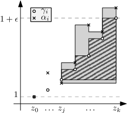
We now lower-bound the overall decrease of the values $\alpha^{\prime}_{i}$’s w.r.t. the corresponding $\alpha_{i}$’s by using the following inequalities (see Figure 3):

The above selection procedure is repeated by the algorithm for every failed edge $e_{h}$ and for every corresponding bad vertex. We now focus on the $h$-th phase of the algorithm. We call $B_{h}$ the set of all the bad vertices considered in this phase and, for every $t\in B_{h}$, we call $U(t)$ the corresponding set $U$, as defined above. Moreover, let $U_{h}=\cup_{t\in B}U(t)$, and let $V_{h}=\bigcup_{i=1}^{h}U_{i}$ (notice that $V_{0}=\emptyset$). Notice that the sets $U(t)$ are pairwise disjoint since, once $z\in U(t)$ we add the edge of $\pi^{-e}(t)$ entering $z$ and hence $z$ cannot belong to any other set $U(t^{\prime})$ where $t^{\prime}$ is a bad vertex which is considered after $t$ in phase $h$. Hence, we let $P_{h}(z)$ be the unique path $P(z)$ which is built during phase $h$. Finally, let $H^{\prime}_{h}$, $H(t)$, and $H_{h}$ be the structures built by the algorithm at the beginning of phase $h$, just before the bad vertex $t\in B_{h}$ is processed, and at the end of phase of phase $h$, respectively.

Let $m_{h}$ be the number of new edges added during the phase $h$. We can now prove:

Now, let us define a function $\phi_{h}(z)$, first we set $\phi_{0}(z)=\frac{6}{\varepsilon}d(z)$ for every $z\in V$, and then we recursively define:

We now consider the remaining case:

References

- (1) I. Althöfer, G. Das, D.P. Dobkin, D. Joseph, and J. Soares, On sparse spanners of weighted graphs, Discrete & Computational Geometry, 9:81–-100, 1993.
- (2) G. Ausiello, A. Ribichini, P.G. Franciosa, and G.F. Italiano, Computing graph spanners in small memory: Fault-tolerance and streaming, Discrete Mathematics, Algorithms and Applications, 2(4):591–606, 2010.
- (3) G. Ausiello, P.G. Franciosa, G.F. Italiano, and A. Ribichini, On resilient graph spanners, Proc. of the 21st European Symp. on Algorithms (ESA’13), Vol. 8125 of Lecture Notes in Computer Science, Springer, 85–96, 2013.
- (4) S. Baswana, T. Kavitha, K. Mehlhorn, and S. Pettie, Additive spanners and -spanners, ACM Trans. on Algorithms, 7, A.5, 2010.
- (5) S. Baswana and N. Khanna, Approximate shortest paths avoiding a failed vertex: near optimal data structures for undirected unweighted graphs, Algorithmica, 66(1):18–50, 2013.
- (6) A. Bernstein and D.R. Karger, A nearly optimal oracle for avoiding failed vertices and edges, Proc. of the 41st Symp. on the Theory of Computing (STOC’09), ACM Press, 101–110, 2009.
- (7) D. Bilò, F. Grandoni, L. Gualà, S. Leucci, and G. Proietti, Improved purely additive fault-tolerant spanners, Proc. of the 23rd European Symposium on Algorithms (ESA’15), Vol. 9294 of Lecture Notes in Computer Science, Springer, 167–178, 2015.
- (8) D. Bilò, L. Gualà, S. Leucci, and G. Proietti, Compact and fast sensitivity oracles for single-source distances, Proc. of the 24th Annual European Symposium on Algorithms (ESA’16), Vol. 57 of Leibniz International Proceedings in Informatics (LIPIcs), 13:1–13:14, 2016.
- (9) D. Bilò, L. Gualà, S. Leucci, and G. Proietti, Multiple-edge-fault-tolerant approximate shortest-path trees, Proc. of the 33rd Symposium on Theoretical Aspects of Computer Science (STACS’16), Vol. 47 of Leibniz International Proceedings in Informatics (LIPIcs), 18:1–18:14, 2016.
- (10) G. Braunschvig, S. Chechik, and D. Peleg, Fault tolerant additive spanners, Proc. of the 38th Workshop on Graph-Theoretic Concepts in Computer Science (WG’12), Vol. 7551 of Lecture Notes in Computer Science, Springer, 206–214, 2012.
- (11) S. Chechik, New additive spanners, Proc. of the 24th Symp. on Discrete Algorithms (SODA’13), ACM Press, 498–512, 2013.
- (12) S. Chechik, M. Langberg, D. Peleg, and L. Roditty, Fault-tolerant spanners for general graphs, Proc. of the 41st Symp. on the Theory of Computing (STOC’09), ACM Press, 435–444, 2009.
- (13) S. Chechik, M. Langberg, D. Peleg, and L. Roditty, -sensitivity distance oracles and routing schemes, Proc. of the 18th European Symp. on Algorithms (ESA’10), Vol. 6942 of Lecture Notes in Computer Science, Springer, 84–96, 2010.
- (14) M. Cygan, F. Grandoni, and T. Kavitha, On pairwise spanners, Proc. of the Symp. on Theoretical Aspects of Computer Science (STACS’13), Vol. 20 of Leibniz International Proceedings in Informatics (LIPIcs), 209–220, 2013.
- (15) A. D’Andrea, M. D’Emidio, D. Frigioni, S. Leucci, and G. Proietti, Path-fault-tolerant approximate shortest-path trees, Proc. of the 22nd Int. Coll. on Structural Information and Communication Complexity (SIROCCO’15), Vol. 9439 of Lecture Notes in Computer Science, Springer, 224–238, 2015.
- (16) M. Dinitz and R. Krauthgamer, Fault-tolerant spanners: better and simpler, Proc. of the 30th Symp. on Principles of Distributed Computing (PODC’11), ACM Press, 169–178, 2011.
- (17) R. Duan and S. Pettie, Dual-failure distance and connectivity oracles, Proc. of the 20th Symp. on Discrete Algorithms (SODA’09), ACM Press, 506–515, 2009.
- (18) P. Erdős, Extremal problems in graph theory, Proc. of the Symp. on Theory of Graphs and its Applications, 29–36, 1964.
- (19) F. Grandoni and V. Vassilevska Williams, Improved distance sensitivity oracles via fast single-source replacement paths, Proc. of the 53rd Annual IEEE Symp. on Foundations of Computer Science (FOCS’12), 748–757, 2012.
- (20) E. Nardelli, G. Proietti, and P. Widmayer, Swapping a failing edge of a single source shortest paths tree is good and fast, Algorithmica, 36(4):361–374, 2003.
- (21) M. Parter, Vertex fault tolerant additive spanners, Proc. of the 28th International Symposium on Distributed Computing (DISC’14), Vol. 8784 of Lecture Notes in Computer Science, Springer, 167–181, 2014.
- (22) M. Parter, Dual failure resilient BFS structure, Proc. of the 34th Symp. on Principles of Distributed Computing (PODC’15), ACM Press, 481–490, 2015.
- (23) M. Parter, Fault-Tolerant Logical Network Structures, Bulletin of the EATCS, Vol. 118, 2016.
- (24) M. Parter and D. Peleg, Sparse fault-tolerant BFS trees, Proc. of the 21st European Symp. on Algorithms (ESA’13), Vol. 8125 of Lecture Notes in Computer Science, Springer, 779–790, 2013.
- (25) M. Parter and D. Peleg, Fault tolerant approximate BFS structures, Proc. of the 25th Symp. on Discrete Algorithms (SODA’14), ACM Press, 1073–1092, 2014.