Lattice gases with a point source

We formalize the system with the following rules. The system is initially empty, so that at time $t=0_{+}$ only the origin is occupied.

1. 1.

   One particle, say at site ${\bf x}$, is randomly chosen.

2. 2.

   A nearest-neighbour site of ${\bf x}$, say ${\bf y}$, is randomly chosen.

3. 3.

   If ${\bf y}$ is empty, the particle hops from ${\bf x}$ to ${\bf y}$; otherwise it remains at ${\bf x}$.

4. 4.

   Time advances, $t\leftarrow t+\nicefrac{{1}}{{N}}$, where $N$ is the current number of particles in the system.

5. 5.

   If the chosen particle moved from the origin, ${\bf x}={\bf 0}$, a new particle is added at the origin: $N\leftarrow N+1$.

6. 6.

   Go back to step 1.

These rules, which also represent the core of our numerical simulations, are illustrated in Figure 2.

We first examine the number of injected particles. We use the notation $N_{d}(t)$ for the total number of particles to emphasize the dependence on the spatial dimension $d$. The mean $\langle N_{d}(t)\rangle$ grows [14] as

Here $W_{d}$ are the Watson integrals [31]

where ${\bf q}=(q_{1},\ldots,q_{d})$ and $Q({\bf q})=\frac{2}{d}\sum_{1\leq i\leq d}(1-\cos q_{i})$. For the cubic lattice $\mathbb{Z}^{3}$, the Watson integral has been expressed [32] via Euler’s gamma function $W_{3}=\frac{\sqrt{6}}{64\,\pi^{3}}\,\Gamma\left(\frac{1}{24}\right)\,\Gamma\left(\frac{5}{24}\right)\,\Gamma\left(\frac{7}{24}\right)\,\Gamma\left(\frac{11}{24}\right)=0.75819303\ldots$.

Equation (1) shows that the critical dimension is 2, as for $d>2$ the growth law of $\langle N_{d}\rangle$ becomes universal, namely linear in time. In two dimensions, the difference from the higher-dimensional behaviour is logarithmic, i.e., rather small. We also emphasize that the average total number of injected particles is lattice-independent when $d\leq 2$. The explanation of this behaviour is simple: in one and two dimensions, the density varies on a scale which grows with time, so that the lattice structure is asymptotically irrelevant. For $d\geq 3$, the results are lattice-dependent.

Comparing with simulations,¹¹ 1 Numerical simulations were prototyped in Haskell, and final programs written in C. They were run on a cluster of workstations with a total of 300 cores over a period of 8 months. Figure 3, in one dimension there is excellent agreement both for the $\sqrt{t}$ dependence on the time and for the amplitude:

We now consider the domain of visited sites. In two dimensions, the visited domains in $\mathbb{Z}^{2}$, Figure 1, are fractal-like but remarkably circular. Denote by $R_{1}$, $R_{2}$ the radius of the largest inscribed and the smallest circumscribed disc, respectively. Simulations, Figure 5, suggest that $\frac{R_{2}}{R_{1}}\sim 1+\frac{C}{\ln R_{1}}$. It would be interesting to explore the shape of the visited domain in detail, e.g., to explain this apparent logarithmic decay of the relative width of the annulus, but here we limit ourselves to its volume, the total number of sites each of which has been visited at least once by at least one particle. We will show that the average total number of distinct visited sites $\langle V_{d}\rangle$ grows as

These growth laws indicate that $d^{c}=4$ plays the role of the upper critical dimension.

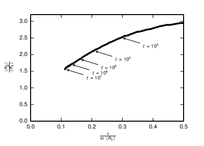
We now provide heuristic arguments in favour of (6). To appreciate the possible time dependence in (6), keep in mind two laws – the growth law (1) for the average total number of particles, and the well-known growth law [2]

for the average total number of distinct sited visited by a single random walker.

There are two obvious lower bounds, $\langle V_{d}\rangle>\langle\mathcal{V}_{d}\rangle$ and $\langle V_{d}\rangle>\langle N_{d}\rangle$, which are essentially identical. There is also a simple upper bound $\langle V_{d}\rangle<\langle\mathcal{V}_{d}\rangle\langle N_{d}\rangle$ (because not all particles are introduced at time zero and moreover the same site can be visited by different particles). Using these bounds and ignoring numerical factors we get

To obtain stronger heuristic predictions we note that during the time interval $(0,t)$ almost all particles in the system never go more than $\sqrt{t}$ away from the origin. This lends support to $\langle V_{d}(t)\rangle\sim t^{d/2}$. This growth law can hold only up to $d=4$, as manifested by the upper bound $\langle V_{d}(t)\rangle<t^{2}$. These arguments suggest that the algebraic dependence on time is

as in (6), leaving the possibility of logarithmic corrections. Theoretical analyses in dimensions $d=1,2,3$ (Section 4) lead to the following specific forms (supported by extensive simulations, Figure 6):

Finally, we consider the total number of arrivals at sites. If the same particle leaves a site and then returns, a return is counted as a new arrival. Denote by $S_{m}(t)$ the total number of sites which have been visited exactly $m$ times during the time interval $(0,t)$. The zeroth moment of the distribution $S_{m}(t)$

is merely the total number of visited sites. The first moment of the distribution $S_{m}(t)$ is also interesting: it characterizes the integrated “activity” of the process, i.e., the total number of arrivals:

A detailed derivation (Section 5) shows that

as confirmed numerically, Figure 7.

The RW model consists of particles undergoing nearest-neighbour symmetric random walks. Similarly to the case of the SEP we assume that a new random walker is immediately deposited at the origin once it becomes empty. Multiple occupancy, however, is allowed. Despite the lack of direct interaction between RWs, there is an implicit collective interaction implied by the input rule: a new RW can be added only when the origin becomes empty, and this depends on all RWs which were present before the deposition event. This makes the process involving RWs non-trivial, and certain features are simpler to compute for the SEP than for the RWs. This can be appreciated by considering the density at the origin. In the case of the SEP, $n_{\bf 0}\equiv 1$ since there is always one particle at the origin. For RWs, the number of particles at the origin is a random variable, so its full description is provided by a probability distribution

For $d=1$ and $d=2$, the probability distribution (14) continues to evolve and, e.g., the average occupancy of the origin, $\langle n_{\bf 0}(t)\rangle=\sum_{k\geq 1}kP_{k}(t)$, grows indefinitely, albeit anomalously slowly, see Eq. (17). In higher dimensions, $d\geq 3$, the probability distribution (14) becomes stationary in the large time limit.

A different version of the model where a large but fixed number of RWs is simultaneously released at a single point has been studied in Refs. [9, 11, 12]. This model has been further analysed and generalized in subsequent studies, see e.g., Refs. [33, 34, 35, 36] and references therein. In our setting, the number of RWs grows with time, but one can still adopt the methods of Refs. [9, 11, 12] to investigate, e.g., the average total number of distinct sites visited by RWs.

The RW model is formalized as follows:

1. 1.

   One RW, say at site ${\bf x}$, is randomly chosen, and it hops to a randomly chosen neighbouring site of ${\bf x}$.

2. 2.

   Time advances, $t\leftarrow t+\nicefrac{{1}}{{N}}$, where $N$ is the current number of RWs in the system.

3. 3.

   If the chosen RW was at the origin and it was the only particle at the origin, a new RW is added at the origin: $N\leftarrow N+1$.

4. 4.

   Go back to step 1.

Our analytical approach is non-rigorous, but emerging results appear to be asymptotically exact. We emphasize that, in our set-up, the addition of the new RW at the origin is ultimately related to the previous history of the process, so there is an effective interaction. The analysis is more difficult than in the case of the SEP where the number of particles at the origin is fixed, $n_{\bf 0}\equiv 1$.

If the average density $\langle n_{\bf 0}\rangle$ at the origin were known, then

with $\langle N_{d}\rangle$ corresponding to the SEP, where $\langle n_{\bf 0}\rangle\equiv 1$, and hence given by (1). Let us assume that $\langle n_{\bf 0}\rangle$ is a slowly varying function of time; we will confirm this assumption a posteriori. Thus the distribution (14) is essentially an equilibrium distribution with average density $\langle n_{\bf 0}\rangle$. It proves convenient to consider the case of finite flux, even small flux $F\ll 1$, when the additions of new particles are rare and the distribution (14) is the Poisson distribution. In that case we have $P(0,t)=e^{-\langle n_{\bf 0}\rangle}$, and hence the average total number of particles increases according to the rate equation

Using (15) and (1) we get $\frac{d}{dt}\langle N_{1}^{\text{RW}}\rangle\simeq\langle n_{\bf 0}\rangle/\sqrt{\pi t/2}$ in one dimension. Substituting this into (16) we obtain $\langle n_{\bf 0}\rangle\simeq\frac{1}{2}\ln t$. The leading asymptotic does not depend on the flux, and hence we anticipate that the prediction for $\langle n_{\bf 0}\rangle$ remains correct for large flux, and in the most interesting case of the infinite flux (into the empty origin). A more accurate derivation for the case of the infinite flux (Section 3.3) confirms the $\langle n_{\bf 0}\rangle\simeq\frac{1}{2}\ln t$ asymptotic.

In two dimensions we similarly find

from which $\langle n_{\bf 0}\rangle\simeq\ln(\ln t)$.

When $d\geq 3$, the average density at the origin approaches $2W_{d}[2W_{d}-1]^{-1}\ln(2W_{d})$, as we show in Section 3.3. Thus the average density at the origin reads

For the cubic lattice, $\langle n_{{\bf 0}3}\rangle=1.222567616\ldots$; see Figure 8. The average total number of particles grows as

Hereinafter we write $\langle N_{d}\rangle$ instead of $\langle N_{d}^{\text{RW}}\rangle$ when there is no danger of misinterpretation.

In one and two dimensions, the sub-leading terms are only formally negligible; in practice they are almost as large as the leading terms. Indeed, repeating the above analysis and trying to keep sub-leading terms, one gets

in one dimension. The amplitude $C_{2}$ is very difficult to compute, and even if we were able to compute it, the following sub-sub-leading term which is not displayed in (19) will involve an even nastier repeated logarithm: $\ln\ln\ln t$. Ignoring these difficult-to-compute corrections, we get surprisingly good agreement:

Similarly in two dimensions

with unknown amplitude $C_{3}$. The appearance of repeated logarithms makes it doubtful that one can confirm heuristic predictions for the leading terms.

In three dimensions, the linear growth with time is in excellent agreement with simulation results. As for the amplitude, the theoretical prediction is

Numerically the amplitude is approximately $0.81$; see Figure 9.

The probability distribution (14) describing RWs at the origin satisfies

for $k\geq 2$ and

Here $\mu$ is the average density on the sites neighbouring the origin. In the long time limit we can neglect the terms on the left-hand side of Eqs. (23)–(24). This is obvious when $d\geq 3$, since in this case the probability distribution reaches a stationary state. When $d=1$ or $d=2$, the left-hand sides can be ignored in the realm of a quasi-stationary approximation; one can make such an assumption, find a solution, and justify the quasi-stationary approximation a posteriori.

Solving the stationary version of (24) and then the following equations (23) we find $P_{k}=P_{1}\,\mu^{k-1}/k!$ and fix $P_{1}$ through the normalization $\sum_{k\geq 1}P_{k}=1$ to yield

For $d\geq 3$, we have

Using (25) we find that the average density at the origin

Recall that $n_{\bf 0}/\mu=2W_{d}/(2W_{d}-1)$ in the case of the SEP, see Ref. [6]. The ratio is the same in the case of RWs (as the governing equations for the average densities are identical). Therefore (27) gives

from which $\mu=\ln(2W_{d})$. Substituting this into (27) we establish the announced result (17).

For $d=1$ and $d=2$, the average density at the origin $\langle n_{\bf 0}\rangle$ and the average density $\mu$ on the sites neighbouring the origin both diverge in the long time limit, and asymptotically $\langle n_{\bf 0}\rangle\simeq\mu$ due to (27). Hence (26) becomes

in the leading order. This is a more precise equation than (16), yet it yields the same leading asymptotic.

In one dimension, it suffices to study the one-sided problem. We wish to compute the probability $\Pi(L,t)$ that the particles never went beyond distance $L$ during the time interval $(0,t)$. To this end we put an artificial boundary at $x=L$. Mathematically, we must solve the diffusion equation

on the interval $0\leq x\leq L$. The initial condition is

and the absorbing boundary condition

For the SEP, there is another boundary condition

modelling the source. The probability $\Pi(L,t)$ is then

The probability that the distance is exactly $L$ is given by $\frac{\partial\Pi}{\partial L}$, and the average distance

The main contribution is gathered in the region

We assume this to hold and justify a posteriori. Using (38) we can simplify the problem, namely we can consider (32) on the real line $-\infty<x<\infty$ subject to the initial condition

Then the absorbing boundary condition (34) is obeyed due to symmetry, while the boundary condition (35) is valid thanks to (38). Solving (32) subject to (39) yields

from which

and therefore

Writing

we recast (41) into

where the second line is the leading asymptotic which applies when $\eta\gg 1$. Substituting (42)–(43) into (37) we compute $\langle L\rangle$ and determine $\langle V_{1}\rangle=2\langle L\rangle+1$

In the large time limit, the integral in (44) approaches $\sqrt{2\zeta}$, where $\zeta$ is a root of

Thus

A root of Eq. (45) is known as the Lambert $W$ function: $\zeta=W(\sqrt{8t/\pi})$. Asymptotically $\zeta\simeq\tfrac{1}{2}\ln t$, and therefore the average total number of visited sites grows as

in agreement with (6). [Equation (47) also gives the announced result (30) for the amplitude in one dimension.] The asymptotic growth (47) is faster than $\sqrt{t}$. This justifies the assumption (38) which was used in the above analysis.

It is difficult to confirm the amplitude $C_{1}=2$ numerically. The solution to Eq. (45) actually reads $\zeta\simeq\tfrac{1}{2}\ln t-\ln(\ln t)+\ldots$, so the approach to the leading asymptotic growth is very slow. One can take (44) as the theoretical prediction, compute the integral numerically as a function of time, and compare the outcome with simulations, Figure 3a.

For RWs, the density is obtained by multiplying the density $\rho(x,T)$ corresponding to the SEP problem by the average density $\tfrac{1}{2}\ln T$ of RWs at the origin. Thus instead of (41) we obtain

and instead of (43) we get

from which

The average number of visited sites is given by the same formula (46) as before, where $\zeta$ is now a root of

which can be written through the Lambert $W$ function: $\zeta=W(\sqrt{2t/\pi}\,\ln t)$. The leading asymptotic is the same as in the case of the SEP, $\zeta\simeq\tfrac{1}{2}\ln t$, and therefore the asymptotic growth is given by the same formula (47). A better approximation is probably provided by (48); see Figure 9a.

Let us try to estimate the discrepancy between the growth of the average total number of visited sites in the case of the SEP and RWs. We have

where $\zeta^{\text{RW}}$ is the solution of (49). Dividing (49) by (45) we obtain $\zeta^{\text{RW}}-\zeta\simeq\ln\!\big(\tfrac{1}{2}\ln t\big)$, and therefore

leading to the announced result (31) for the ratio of effective amplitudes.

Consider first a single RW released at the origin at time $t=0$. The probability that it will visit site ${\bf x}$ during the time interval $(0,t)$ is

where $x^{2}=|{\bf x}|^{2}$ and $D=(2d)^{-1}$ with our choice of the hopping rates. Equation (51) is (asymptotically) exact in the long-time limit, $t\gg 1$, when we can ignore the lattice structure and use the prediction $(4\pi D\tau)^{-d/2}e^{-x^{2}/4D\tau}$ from the continuous approach for the probability to visit site ${\bf x}$ the last time at time $\tau$ before $t$. We then multiply this probability by the persistence probability that the RW does not return to ${\bf x}$ during the time interval $(\tau,t)$ and take into account that this persistence probability saturates at $(2W_{d})^{-1}$ when $d>2$.

When $d>2$, the renormalized flux is finite, so for computing the average number of visits it suffices to assume that RWs are added at a constant rate $\Phi_{d}$; according to (18) the flux is $\Phi_{d}=[2W_{d}-1]^{-1}\ln(2W_{d})$, although the actual value will play a minor role. Thus we release particles at times $0=t_{1}<t_{2}<\cdots<t_{N}=t$ with $N=\Phi_{d}t$. The probability that none of them will visit site ${\bf x}$ is given by $\prod_{1\leq j\leq N}(1-P_{j})$, so the probability that at least one RW will visit site ${\bf x}$ is $1-\prod_{1\leq j\leq N}(1-P_{j})$, and the average number of visited sites is

Using (51) we get

We will see that the dominant contribution to the integral in (52) is gathered in the region where $\xi=\frac{x^{2}}{4Dt}\gg 1$. In this region (53) simplifies to

We now write

Combining this with (54) and computing the asymptotic behaviour of the integral we arrive at

where $\Omega_{d}=2\pi^{\delta}/\Gamma(\delta)$ is the volume of the $(d-1)$-dimensional unit sphere, $\Psi_{d}=(2W_{d})^{-1}\Phi_{d}(\delta/\pi)^{\delta}$, and we use the shorthand notation $\delta=d/2$. The expression in the brackets in the integral in (55) is very close to 1 when $\xi<\xi_{*}$ and it quickly vanishes when $\xi>\xi_{*}$, where $\xi_{*}$ is determined from

The integral is $\int_{0}^{\xi_{*}}d\xi\,\xi^{\delta-1}=\delta^{-1}\xi_{*}^{\delta}$ in the leading order. From (56) we see that $\xi_{*}\simeq(2-\delta)\ln t$, so it diverges when $\delta<2$, i.e. $d<4$. The above analysis assumes that the major contribution to the integrals is gathered when $\xi$ is large, and hence it is justified when $d<4$. Since we also assumed that $d>2$, the results essentially apply only to $d=3$. Specializing to $d=3$ we arrive at

Here instead of $\xi_{*}\simeq\tfrac{1}{2}\ln t$ we used a more precise solution of (56) in three dimensions:

and a more precise expression, viz. $\tfrac{2}{3}\xi_{*}^{3/2}+\gamma\sqrt{\xi_{*}}$ where $\gamma\approx 0.5772$ is the Euler constant, of the integral in (55). We also inserted the constant $\Psi_{3}^{2}$ into the time variable, namely inside the logarithms the time variable is

When $d=4$, there is no sharp crossover, and $\langle V_{4}\rangle\sim t^{2}$ without logarithmic corrections. When $d>4$, we have $\langle V_{d}\rangle\sim t^{2}$ as we already explained above, namely because both the lower and upper bounds scale as $t^{2}$.

The two-dimensional case is more subtle. We can still use (51), but the persistence probability now vanishes: $P_{2}\simeq 1/\ln t$. It vanishes so slowly that we can still use the same quantity $1/\ln t$ independently of the time when the RW was released. We can also ignore the fact that the flux slowly varies with time and merely use $N=\pi t\,\frac{\ln\ln t}{\ln t}$, see (18). Repeating the above analysis we get

The crossover occurs around $\xi_{*}$ which is implicitly determined by

from which $\xi_{*}\simeq\ln t-4\ln(\ln t)+\ln(\ln(\ln t))$. The integral in (58) is $\xi_{*}$ in the leading order. A more precise estimate of the integral is given by

The constant is Euler’s constant due to the identity

Therefore

The growth laws (57) and (59) hint why it is so difficult to extract the true asymptotic behaviours from numerics; see Figure 6.

In physically relevant dimensions, the main contribution to the total number of distinct visited sites is gathered in the region $\xi=\frac{x^{2}}{4Dt}\gg 1$ where the density is small and the difference between RWs and the SEP is negligible. Therefore the leading asymptotic behaviour of $\langle V_{d}\rangle$ is expected to be the same when $d=1,2,3$. Above, this was analysed in more detail for the $d=1$ case. In two dimensions, one anticipates that

leading to

In addition to the average number of visited sites, one would like to compute the full probability distribution. This is a much more challenging problem, especially when $d>1$. Even in one dimension when the visited domain is an interval, the problem is rather challenging and it has been studied only in the situation [9, 36] when the total number of random walks is fixed and they were all simultaneously released. Even in this situation, conditioning the trajectories of the RWs to a given number of visited sites introduces effective correlations between the walkers [36]. In our setting, when the RWs are released throughout the evolution, there are additional correlations which are built to allow injection events, there are fluctuations in the total number of injected RWs, etc. Let us make a bold assumption that these additional effects do not change the behaviour in the leading order. Specializing the results of Ref. [36] to our setting yields the probability distribution

with the scaled probability distribution given by

where $K_{0}$ is the modified Bessel function.

References

- [1] H. C. Berg, Random Walks in Biology. Princeton, NJ: Princeton University Press, 1993.
- [2] G. H. Weiss, Aspects and Applications of the Random Walk. Amsterdam: North-Holland, 1994.
- [3] A. B. Kolomeisky and M. E. Fisher, “Molecular motors: a theorist’s perspective,” Annual Reviews of Physical Chemistry, vol. 58, pp. 675–695, 2007.
- [4] P. L. Krapivsky, S. Redner, and E. Ben-Naim, A Kinetic View of Statistical Physics. Cambridge: Cambridge University Press, 2010.
- [5] G. M. Viswanathan, M. G. E. da Luz, E. P. Raposo, and H. E. Stanley, The Physics of Foraging: An Introduction to Random Searches and Biological Encounters. Cambridge University Press, 2011.
- [6] P. L. Krapivsky, “Kinetics of monomer-monomer surface catalytic reactions,” Phys. Rev. A, vol. 45, pp. 1067–1072, 1992.
- [7] L. Frachebourg and P. L. Krapivsky, “Exact results for kinetics of catalytic reactions,” Phys. Rev. E, vol. 53, pp. R3009–R3012, 1996.
- [8] M. Mobilia, “Does a single zealot affect an infinite group of voters?,” Phys. Rev. Lett., vol. 91, p. 028701, 2003.
- [9] H. Larralde, P. Trunfio, S. Havlin, H. E. Stanley, and G. H. Weiss, “Territory covered by diffusing particles,” Nature, vol. 355, pp. 423–426, 1992.
- [10] H. Larralde, P. Trunfio, S. Havlin, H. E. Stanley, and G. H. Weiss, “Number of distinct sites visited by random walkers,” Phys. Rev. A, vol. 45, no. 10, pp. 7128–7138, 1992.
- [11] G. M. Sastry and N. Agmon, “The span of one-dimensional multiparticle Brownian motion,” J. Chem. Phys., vol. 104, no. 8, pp. 3022–3025, 1996.
- [12] S. B. Yuste and L. Acedo, “Territory covered by random walkers,” Phys. Rev. E, vol. 60, pp. R3459–R3462, 1999.
- [13] S. B. Yuste and L. Acedo, “Number of distinct sites visited by random walkers on a Euclidean lattice,” Phys. Rev. E, vol. 61, pp. 2340–2347, 2000.
- [14] P. L. Krapivsky, “Symmetric exclusion process with a localized source,” Phys. Rev. E, vol. 86, no. 041103, 2012.
- [15] H. Spohn, Large Scale Dynamics of Interacting Particles. New York: Springer, 1991.
- [16] C. Kipnis and C. Landim, Scaling Limits of Interacting Particle Systems. New York: Springer, 1999.
- [17] T. M. Liggett, Stochastic Interacting Systems: Contact, Voter, and Exclusion Processes. New York: Springer, 1999.
- [18] G. M. Schütz, “Exactly solvable models for many-body systems far from equilibrium,” in Phase Transitions and Critical Phenomena (C. Domb and J. L. Lebowitz, eds.), London: Academic Press, 2000.
- [19] R. A. Blythe and M. R. Evans, “Nonequilibrium steady states of matrix-product form: a solver’s guide,” J. Phys. A, vol. 40, p. R333, 2007.
- [20] B. Derrida, “Non-equilibrium steady states: fluctuations and large deviations of the density and of the current,” J. Stat. Mech., p. P07023, 2007.
- [21] T. Chou, K. Mallick, and R. K. P. Zia, “Non-equilibrium statistical mechanics: From a paradigmatic model to biological transport,” Reports on Progress in Physics, vol. 75, p. 116601, 2011.
- [22] M. N. Popescu, G. Oshanin, S. Dietrich, and A.-M. Cazabat, “Precursor films in wetting phenomena,” J. Phys.: Condens. Matter, vol. 24, p. 243102, 2012.
- [23] S. F. Burlatsky, G. Oshanin, A. M. Cazabat, and M. Moreau, “Microscopic model of upward creep of an ultrathin wetting film,” Phys. Rev. Lett., vol. 76, pp. 86–89, 1996.
- [24] S. F. Burlatsky, G. Oshanin, A. M. Cazabat, M. Moreau, and W. P. Reinhard, “Spreading of a thin wetting film: Microscopic approach,” Phys. Rev. E, vol. 54, pp. 3832–3845, 1996.
- [25] O. Semenov, D. Mohr, and D. Stefanovic, “First-passage time properties of multivalent catalytic walkers,” Phys. Rev. E, vol. 88, p. 012724, 2013.
- [26] R. Pei, S. K. Taylor, D. Stefanovic, S. Rudchenko, T. E. Mitchell, and M. N. Stojanovic, “Behavior of polycatalytic assemblies in a substrate-displaying matrix,” J. Am. Chem. Soc., vol. 39, no. 128, pp. 12693–12699, 2006.
- [27] K. Lund, A. J. Manzo, N. Dabby, N. Michelotti, A. Johnson-Buck, J. Nangreave, S. Taylor, R. Pei, M. N. Stojanovic, N. G. Walter, E. Winfree, and H. Yan, “Molecular robots guided by prescriptive landscapes,” Nature, vol. 465, pp. 206–210, May 2010.
- [28] T. Antal and P. L. Krapivsky, “Molecular spiders with memory,” Physical Review E, vol. 76, no. 2, p. 021121, 2007.
- [29] O. Semenov, M. J. Olah, and D. Stefanovic, “Mechanism of diffusive transport in molecular spider models,” Physical Review E, vol. 83, p. 021117, Feb. 2011.
- [30] M. J. Olah and D. Stefanovic, “Superdiffusive transport by multivalent molecular walkers moving under load,” Phys. Rev. E, vol. 87, p. 062713, 2013.
- [31] G. N. Watson, “Three triple integrals,” Quart. J. Math. (Oxford), vol. os-10, no. 1, pp. 266–276, 1939.
- [32] M. L. Glasser and I. J. Zucker, “Extended Watson integrals for the cubic lattices,” Proc. Nat. Acad. Sci. U.S.A., vol. 74, no. 5, pp. 1800–1801, 1977.
- [33] J. Dräger and J. Klafter, “Sorting single events: Mean arrival times of N random walkers,” Phys. Rev. E, vol. 60, p. 6503, 1999.
- [34] E. Arapaki, P. Argyrakis, and A. Bunde, “Diffusion-driven spreading phenomena: The structure of the hull of the visited territory,” Phys. Rev. E, vol. 69, p. 031101, 2004.
- [35] S. N. Majumdar and M. V. Tamm, “Number of common sites visited by N random walkers,” Phys. Rev. E, vol. 86, p. 021135, 2012.
- [36] A. Kundu, S. N. Majumdar, and G. Schehr, “Exact distributions of the number of distinct and common sites visited by N independent random walkers,” Phys. Rev. Lett., vol. 110, p. 220602, 2013.
- [37] C. Appert-Rolland, B. Derrida, V. Lecomte, and F. van Wijland, “Universal cumulants of the current in diffusive systems on a ring,” Phys. Rev. E, vol. 78, p. 021122, Aug 2008.
- [38] B. Mandelbrot, The Fractal Geometry of Nature. San Francisco: W. H. Freeman, 1982.
- [39] G. F. Lawler, O. Schramm, and W. Werner, “The dimension of the planar brownian frontier is 4/3,” Math. Research Lett., vol. 8, p. 401, 2001.
- [40] F. V. Wijland, S. Caser, and H. J. Hilhorst, “Statistical properties of the set of sites visited by the two-dimensional random walk,” J. Phys. A, vol. 30, p. 507, 1997.
- [41] F. V. Wijland and H. J. Hilhorst, “Universal fluctuations in the support of the random walk,” J. Stat. Phys., vol. 89, p. 119, 1997.