Maximizing Protein Translation Rate in the Ribosome Flow Model: the Homogeneous CaseThanks: This research is partially supported by research grants from the ISF and from the Ela Kodesz Institute for Medical Engineering and Physical Sciences.
Abstract
Gene translation is the process in which intracellular macro-molecules, called ribosomes, decode genetic information in the mRNA chain into the corresponding proteins. Gene translation includes several steps. During the elongation step, ribosomes move along the mRNA in a sequential manner and link amino-acids together in the corresponding order to produce the proteins.
The homogeneous ribosome flow model (HRFM) is a deterministic computational model for translation-elongation under the assumption of constant elongation rates along the mRNA chain. The HRFM is described by a set of first-order nonlinear ordinary differential equations, where represents the number of sites along the mRNA chain. The HRFM also includes two positive parameters: ribosomal initiation rate and the (constant) elongation rate.
In this paper, we show that the steady-state translation rate in the HRFM is a concave function of its parameters. This means that the problem of determining the parameter values that maximize the translation rate is relatively simple. Our results may contribute to a better understanding of the mechanisms and evolution of translation-elongation. We demonstrate this by using the theoretical results to estimate the initiation rate in M. musculus embryonic stem cell. The underlying assumption is that evolution optimized the translation mechanism.
For the infinite-dimensional HRFM, we derive a closed-form solution to the problem of determining the initiation and transition rates that maximize the protein translation rate. We show that these expressions provide good approximations for the optimal values in the -dimensional HRFM already for relatively small values of . These results may have applications for synthetic biology where an important problem is to re-engineer genomic systems in order to maximize the protein production rate.
Index Terms:
Systems biology, synthetic biology, gene translation, maximizing protein production rate, convex optimization, continued fractions.I Introduction
Proteins are micro-molecules involved in all intracellular activities. DNA regions, called genes, encode proteins as ordered lists of amino acids. During the process of gene expression these regions are first transcribed into mRNA molecules. In the next step, called gene translation, the information encoded in the mRNA is translated into proteins by molecular machines called ribosomes that move along the mRNA sequence [1]. During the translation process, each triplet of consecutive nucleotides, called a codon, is decoded by a ribosome into a suitable amino-acid.
Gene translation is a fundamental cellular process and its study has important implications to numerous scientific disciplines ranging from human health to evolutionary biology. Computational models of translation are becoming increasingly more important due to the need to integrate, analyze, and understand the rapidly accumulating biological findings related to translation [54, 10, 17, 29, 50, 49, 8].
Computational models of translation are also of importance in synthetic biology. Indeed, a major challenge in this field is to re-engineer genomic systems to produce a desired protein translation rate. Computational models of translation are crucial in achieving this goal, as they allow to simulate and analyze the effect of various manipulations of the genomic mechanism on the translation rate.
A standard mathematical model for translation-elongation is the Totally Asymmetric Simple Exclusion Process (TASEP) [45, 55, 24, 7]. TASEP is a stochastic model for particles moving along a track. A chain of sites models the tracks. Each site can be either empty or occupied by a particle. The term simple exclusion refers to the fact that particles hop randomly from one site to the next, but only if the target site is not already occupied. In this way, TASEP encapsulates the interaction between the particles. The term totally asymmetric is used to indicate unidirectional motion along the lattice. Despite its rather simple description, it seems that rigorous analysis of TASEP is non-trivial. See [42] for a detailed exposition of these issues.
In 2011, Reuveni et al. [40] considered a deterministic mathematical model for translation-elongation called the ribosome flow model (RFM). This model may be derived as a mean-field approximation of TASEP (see, e.g. [4, p. R345]).
Recent biological studies have shown that in some cases the elongation rates along the mRNA are approximately constant [19, 39]. Under the assumption of constant elongation rates, the RFM becomes the homogeneous ribosome flow model (HRFM) [32]. This model includes two positive parameters: the initiation rate and the constant elongation rate . In this paper, we show that the steady-state translation rate in the HRFM is a concave function of these parameters. This implies that the problem of optimizing the translation rate under a simple constraint on the rates is a convex optimization problem. Thus, this problem admits a unique solution, and this solution can be easily found (numerically) using simple and efficient algorithms. We also derive an explicit expression for the optimal solution for the particular case of the infinite-dimensional HRFM, that is, when .
These results may have important applications in the context of synthetic biology. Indeed, a fundamental problem in this field is to re-engineer a genetic system by manipulating the transcript sequence, and possibly other intra-cellular variables, in order to maximize the translation rate. Also, it is reasonable to expect that in most organisms evolutionary forces act to optimize translation costs. For example, in micro-organisms the growth rate is globally strongly dependent on the translation rate/efficiency (see, for example, [23, 48, 12, 13]). In addition, it has been shown that in all organisms highly expressed genes undergo selection for sequence features that improve their translation rate efficiency (see, for example, [23, 48, 27]). The mathematical results described here may be applied to study these issues in a rigorous manner.
Concavity of the translation rate with respect to various variables can also be examined experimentally. A recent paper [15] studied the effect of the intracellular translation factor abundance on protein synthesis. Experiments based on a tet07 construct were used to manipulate the production of the encoded translation factor to a sub-wild-type level [15], and measure the translation rate, or protein levels, for each level of the translation factor(s). Their results suggest that the mapping from levels of translation factors to translation rate is indeed concave (see Fig. in [15]). Our results thus provide the first mathematical support of the observed concavity in the experiments of [15].
The remainder of this paper is organized as follows. Section II briefly reviews the RFM and HRFM. Section III presents the main results. Section IV describes an application of the theoretical results for estimating the initiation rate in M. musculus embryonic stem cell. The underlying assumption is that evolution optimized the translation mechanism. The final section summarizes and describes several possible directions for further research. In order to streamline the presentation, all the proofs are placed in the Appendix.
II Preliminaries
In the RFM, mRNA molecules are coarse-grained into consecutive sites. The RFM is given by first-order nonlinear ordinary differential equations:
| (1) | ||||
Here, is the occupancy level at site at time , normalized so that [] implies that site is completely empty [completely full] at time . The parameter is the initiation rate into the chain, and is a parameter that controls the transition rate from site to site . In particular, controls the output rate at the end of the chain.
The rate of ribosome flow into the system is . The rate of ribosome flow exiting the last site, i.e., the protein translation rate, is . The rate of ribosome flow from site to site is (see Fig. 1). Note that this rate increases with (i.e., when site is fuller) and decreases with (i.e., when the consecutive site is becoming fuller). In this way, the RFM, just like the TASEP, takes into account the interaction between the ribosomes in consecutive sites.
Let denote the solution of the RFM at time for the initial condition . Since the state-variables correspond to normalized occupation levels, we always consider initial conditions in the closed -dimensional unit cube: It is straightforward to verify that this implies that for all (see [33]).
Let denote the interior of . It was shown in [33] that the RFM is a monotone dynamical system [46] and that this implies that (1) admits a unique equilibrium point . Furthermore, for all . This means that all trajectories converge to the steady-state . From a biological viewpoint, this means that the ribosome distribution profile along the chain converges to a steady-state profile that does not depend on the initial profile, but only on the parameter values.
We note in passing that monotone dynamical systems have recently found many applications in systems biology, see e.g. [2, 26, 47] and the references therein.
Let
| (2) |
denote the steady-state translation rate. An important problem is to understand the dependence of and, in particular, on the RFM parameters. For the left-hand side of all the equations in (1) is zero, so
| (3) | ||||
This yields
| (4) |
where we define . Also,
| (5) | ||||
and
| (6) |
Combining (5) and (6) provides a finite continued fraction [28] expression for :
| (7) |
Note that (7) has multiple solutions for (and thus also multiple solutions for , however, we are interested only in the unique feasible solution, i.e. the solution corresponding to .
Recent biological findings suggest that in some cases the transition rate along the mRNA chain is approximately constant [19]; this may be also the case for gene transcription [14]. To model this case, Ref. [32] has considered the RFM in the special case where
| (8) |
that is, the transition rates are all equal, and denotes their common value. Since this Homogeneous Ribosome Flow Model (HRFM) includes only two parameters, and , the analysis is simplified. In particular, (7) becomes
| (9) |
where appears a total of times. Note that the right-hand side here is a 1-periodic continued fraction [28]. Eq. (9) yields a polynomial equation of degree in . For example, for Eq. (9) becomes
| (10) |
Several recent papers analyzed the RFM/HRFM. In [31] it has been shown that the state-variables (and thus the translation rate) in the RFM entrain to periodically time-varying initiation and/or transition rates. This provides a computational framework for studying entrainment to a periodic excitation, e.g., the hours solar day or the cell-cycle, at the genetic level. Ref. [34] has considered the RFM with positive linear feedback as a model for ribosome recycling. It has been shown that the closed-loop system admits a unique globally asymptotically stable equilibrium point. Ref. [53] has considered the HRFM in the case of an infinitely-long chain, (i.e. when ) and derived a simple expression for , as well as bounds for for all .
Summarizing, the RFM is a deterministic model for translation-elongation, and perhaps also other stages of gene expression [56, 14], that is highly amenable to analysis.
In the HRFM, the steady-state translation rate is a function of the positive parameters , i.e. . In this paper, we study the dependence of on these parameters.
III Main results
Our first result shows that is a concave function.
III-A Concavity
Theorem 1
Consider the HRFM with dimension . The steady-state translation rate is a concave function on .
The next example demonstrates Theorem 1 for the particular case .
Example 1
Consider the HRFM with . In this case, the feasible solution of (5) and (6) (i.e., the solution satisfying for all ) is
| (11) |
so
| (12) |
It is useful to demonstrate Theorem 1 for this special case. By (12), Note that this implies that . Differentiating again and simplifying yields Similarly, , and Thus, the Hessian matrix of is
| (13) | ||||
where . The eigenvalues of are and . Recall that a twice differentiable function is a concave function of its parameters if and only if its Hessian matrix is negative semidefinite (see e.g. [6]), i.e. if and only if all its eigenvalues are non-positive. It follows that for the mapping is concave. Fig. 2 depicts in (12) as a function of its arguments. It may be seen that this is indeed a concave function.

Example 2
Consider the HRFM with , i.e. with the length of the chain going to infinity. As shown in [53], in this case exists and satisfies
| (14) |
In view of Theorem 1, we expect to be a concave function. Indeed, this may be observed from Fig. 3 that depicts as a function of its variables. This could also be verified analytically from (14).

Recall that a function is called positively homogeneous if for all and all . Since in (7) always appears in a term in the form , it follows that in the RFM is positively homogeneous. In other words,
| (15) |
From a biophysical point of view this means that scaling the initiation rate and all the transition rates by the same multiplicative factor in the RFM yields an increase of the steady-state translation rate by a factor of .
Recall that a function is called superadditive if for all . It is well-known that for a positively homogeneous function, concavity is equivalent to superadditivity (see, e.g., [3]). Combining this with Theorem 1 yields the following result.
Corollary 1
Consider the HRFM with dimension . The function is superadditive on .
This means that
for all . From a biophysical point of view this means the following. Consider two HRFMs, one with initiation rate and transition rate , and the second with initiation rate and transition rate . The total production rate of these two HRFMs is smaller or equal than the production rate of a single HRFM with parameters and .
III-B Maximizing translation rate
Consider the problem of determining the parameter values that maximize or, equivalently, that minimize , in the HRFM. Obviously, to make this problem meaningful we must constrain the possible parameter values. This leads to the following optimization problem.
Problem 1
Given the parameters , minimize , with respect to its parameters and , subject to the constraints:
| (16) | ||||
In other words, the problem is to maximize the protein translation rate under an affine constraint on the total available “resources”, namely, the initiation rate and the common transition rate . The constraint on [] may be related, among others, to the number of intracellular ribosomes [number of intracellular tRNA molecules]. The values of can be used to provide a different weighting to these two resources.
Theorem 1 implies that Problem 1 is a convex optimization problem [6]. It thus benefits from many desirable properties. In particular, it always admits a solution , and it can be solved numerically using efficient algorithms.
The next result shows that increasing or can only increase the translation rate.
Proposition 1
Consider the HRFM with . Then , and
Remark 1
Note that this implies that the first constraint in (16) can always be replaced by
| (17) |
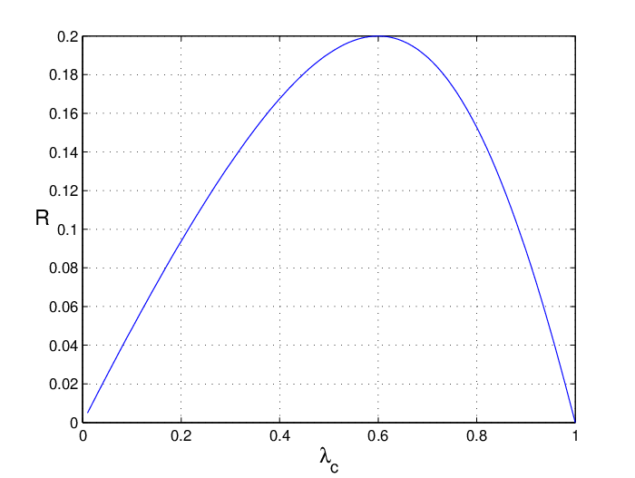
Example 3
Consider Problem 1 for the HRFM with dimension , and with , i.e. the constraint is
| (18) |
Substituting this in (12) yields
Fig. 4 depicts as a function of . It may be seen that when , as a zero transition rate means zero translation rate, and also when , as then the initiation rate is . The maximal value, , is obtained for , so .
In general, one cannot expect an algebraic expression for in terms of . This is true already for the case (see (12)). Surprisingly, perhaps, it is possible to give an algebraic expression for the optimal value as a function of the optimal parameter values and the parameters in the affine constraint.
Theorem 2
Consider Problem 1 for the HRFM with . Then
| (19) |
Example 4
When the dimension of the HRFM goes to infinity we can say much more about the optimal solution.
III-C Optimizing the infinite-dimensional HRFM
Proposition 2
Consider Problem 1 for the infinite-dimensional HRFM. The optimal values are given by
| (20) |
In other words, for we have simple closed-form expressions for the solution of Problem 1 in terms of the constraint parameters , , and .
The expression in (20) shows that increases linearly with . This is reasonable, as increasing corresponds to allowing larger values of and .
Fig. 5 depicts as a function of and . It may be observed that for large values of either or the optimal value decreases quickly. This is reasonable, as a large value of [] implies a tight constraint on [], and decreasing any one of these rates implies a small translation rate. On the other-hand, when both and go to zero, increases quickly.

Let . Then it follows from (20) that
| (21) |
Thus, the ratio is a strictly increasing and concave function of . Note that (21) also implies that . In other words, in the infinite-dimensional HRFM the optimal transition rate is always at least twice as big as the initiation rate.
The parameters and in the optimization problem are upper-bounded by and respectively (see (16)). It follows from (20) that
The case implies that there is no constraint on and thus . Also, the maximal possible value for is . This becomes the rate limiting factor so . When the constraint (17) yields . Also, in this case and the ratio in (21) attains its minimal value, namely, , so .
It turns out that the expressions in (20) actually provide good approximations for the optimal parameter values in finite-dimensional HRFMs. The next example demonstrates this.
Example 5
Consider Problem 1 for the HRFM with , and . Applying a simple numerical algorithm to solve Problem 1 yields
(all numbers are to four digit accuracy). On the other-hand, for Eq. (20) yields
Thus, the optimal values for the infinite-dimensional HRFM agree well with the optimal values already for the -dimensional HRFM.
It is important to note that the typical length of mRNA sequences is larger than sites. For example, in S. cerevisiae the mean length is about sites; in mammals the mRNA chains are much longer; thus, the closed-form asymptotic results here provide a good approximation for the optimal parameter values in finite-dimensional HRFM models of gene translation.
IV A biological example
There exist effective experimental approaches for estimating the translation-elongation rates and the protein synthesis rate, but currently there is no experimental approach for measuring the initiation rate. Indeed, initiation is a highly complex mechanism and its efficiency is based on numerous biophysical properties of the coding sequence including: the nucleotide context of the START codon (i.e., the first codon that is translated in a gene) [22, 57]; the folding of the RNA near the beginning of the open reading frame (ORF) and the nucleotide composition in this region [57, 51]; the number of ribosomes and mRNA molecules in the cell; the length and the nucleotide context of the 5’UTR; interaction between initiation and elongation steps [57, 51], and more. Thus, although there exist experimental approaches for measuring positions on the mRNA suspected to correspond to initiation sites [19, 25], there are no large scale direct measurements of initiation rate.
Several papers addressed the problem of estimating the initiation rate using computational models of translation [53, 41, 9]. One possible application of our results is to estimate the initiation rate based on measurements of elongation and translation rates. Indeed, we may assume, without loss of generality, that . Then, given and , we can determine based on (20). Plugging back in (20) yields the initiation rate . The underlying assumptions here are that the mRNA chain is relatively long; that all elongation rates are equal; and that the parameters of the translation process are indeed optimized by evolution.
To demonstrate this we consider a specific example. Ingolia et al. [19] estimated the constant transition rate in M. musculus embryonic stem cell by applying cyclohexamide to halt translation, and harringtonin to halt initiation at different time steps. This allows estimating the speed of elongation by measuring the movement of the “ribosomal density wave”. They concluded that in mouse embryonic cells codons are translated per second (in terms of the HRFM, this corresponds to sites per second (all numbers are to four digit accuracy), as a ribosome spans about codons [18]). According to [19], this elongation speed is typical, and does not vary much between different genes.
A recent study by Schwanhausser et al. [43] estimated the translation rate in M. musculus fibroblasts by simultaneously measuring protein abundance and turnover by parallel metabolic pulse labeling for more than genes in mouse. They found that the median translation rate in mouse is about proteins per mRNA per hour (i.e., proteins per mRNA per second).
Summarizing, in terms of the HRFM these biological findings suggest that and . To estimate the initiation rate in mouse, we plug these values (and ) in (20). This yields or . The first case is impossible, as in our optimization problem the s must be positive, so we conclude that these values correspond to a solution of Problem 1 with . Applying (20) with these values yields sites per second. This corresponds to codons per second. Note that this agrees well with the estimate in [53] that was obtained using (14). However, the approach here is based on a different argument, namely, that evolution shaped the parameters of the translation process so that they correspond to an optimal solution for Problem 1.
V Discussion and Conclusion
The RFM is a deterministic computational model for ribosome flow along the mRNA. It may be viewed as a mean-field approximation of the stochastic TASEP model and in particular encapsulates both the simple exclusion and the total asymmetry properties of TASEP.
The RFM is characterized by an order , corresponding to the number of sites along the mRNA chain, a positive initiation rate and a set of positive transition rates . Under the assumption (or approximation) of equal transition rates (i.e. ), the RFM becomes the HRFM. Recent studies have suggested that this is the case in some organisms/conditions [19, 39].
In this paper, we showed that in the HRFM the steady-state translation rate is a concave function of its parameters. This implies that a local maximum of is the global maximum. Furthermore, this allows posing the problem of maximizing the steady-state translation rate in a meaningful way as a convex optimization problem. Such problems can be solved using efficient numerical algorithms (see, e.g., [11, 21, 5]).
We also provide an explicit algebraic expression for the optimal translation rate in terms of the optimal parameter values , and the parameters in the affine constraint and , as well as an explicit solution to the convex optimization problem in the infinite-dimensional HRFM.
The reported results may potentially be used for re-engineering gene expression for various biotechnological applications. Specifically, an important problem is to optimize the translation efficiency and protein levels of heterologous genes in a new host [36, 48, 16, 20]. In Section IV we show how and can be estimated. The idea is to use the explicit equations for , and in the infinite-dimensional HRFM. We show that based on experimental measurements of the elongation rates (), and translation rates (), we can estimate and . The underlying assumptions for this approach are that: (1) evolution optimized the translation process; and (2) the mRNA chain is relatively long. In addition, we would like to emphasize that in the case of biotechnological engineering of gene translation, and may be evaluated based on intra-cellular measurement of the concentration and metabolic costs of proteins and genes related to the translation machinery such as initiation factors, elongation factors, tRNA molecules, aminoacyl-tRNA synthetases, etc; these values are related to the ’cost’ of increasing and .
Our results may also be related to the evolution of gene expression, and specifically translation and transcript sequences. Indeed, translation is the process consuming most of the cell energy [36, 48, 1], and it is reasonable to assume that for organisms under strong evolutionary pressure, evolution shapes the genomic machinery so that it optimizes the protein translation rate for the given finite resources.
A natural topic for further research is whether the steady-state translation rate in the RFM is a concave function of its parameters. This question seems to be technically more demanding, as the Hessian matrix of the -dimensional RFM has dimensions , whereas that of the HRFM is . A more general question is related to the concavity of other models of translation including various versions of the TASEP model [34, 50, 48, 44, 8, 38].
More generally, the asymmetric simple exclusion process (ASEP) has become the “default stochastic model for transport phenomena” [52], and has been used to model and analyze many important natural and artificial processes [42]. We believe that the RFM and the HRFM can also be applied to model and analyze more natural and artificial processes.
Acknowledgements
We thank the anonymous reviewers for their helpful comments.
Appendix – Proofs
Proof of Theorem 1. The proof is based on analyzing the Hessian matrix of . Define the normalized initiation rate by
Then we can rewrite (9) as
| (22) |
with
| (23) |
where on the right-hand side appears times. Note that is not necessarily well-defined for all . For example,
is not well-defined for .
Eq. (22) implies that , and since ,
The following results are needed to prove Theorem 1.
Proposition 3
Fix arbitrary and . Let . Then for all the functions , and are well-defined and satisfy
| (24) |
In other words, for all the function is positive, strictly decreasing, and concave.
Example 6

Proof of Proposition 3. Pick . The proof is by induction on . For , , so for all . By (11),
so . Differentiating yields
Thus for , Eq. (24) holds for all .
For the induction step, it is useful to let denote the equilibrium point of the -dimensional HRFM, and let denote the equilibrium point of the -dimensional HRFM. It was shown in [53, Proposition 1] that
| (25) |
In other words, for two HRFM chains with the same the translation rate in the longer chain is smaller than the translation rate in the shorter chain. Assume that (24) holds for all . By (23),
| (26) |
By the induction hypothesis, for all , so is well-defined for all . Differentiating (26) yields
| (27) |
Combining this with the induction hypothesis implies that the right-hand side of (27) is well-defined and strictly negative for all , so in particular
| (28) |
We now show that
| (29) |
Seeking a contradiction, assume that (29) does not hold. Then since , there exists a minimal such that . Combining this with (28) implies that . But since is the equilibrium point of the -dimensional HRFM, , so . This contradiction proves (29).
Differentiating (27) yields
and using (27) yields
| (30) |
We already know that for all and combining this with the induction hypothesis implies that
| (31) |
Combining (29), (28), (31), and (25) completes the proof of the induction step.
Proposition 4
Fix an arbitrary . Let be the function such that . Then
| (32) |
for all .
In other words, the mapping is strictly increasing and concave.
Proof of Proposition 4. We can write (22) as a polynomial equation in with coefficients that are smooth functions of . It is possible to show that the feasible (i.e. the one corresponding to the solution ) is a simple root of this polynomial for all [37]. Hence, is a smooth function.
Rewriting (22) as and differentiating with respect to yields
| (33) |
Combining this with Proposition 3 implies that . Differentiating (33) with respect to yields
Combining this with the fact that and Proposition 3 implies that , and this completes the proof of Proposition 4.
We can now complete the proof of Theorem 1. Differentiating with respect to yields
| (34) |
and
Similarly,
| (35) | ||||
Substituting these expressions in the Hessian matrix (13) yields
A calculation shows that the eigenvalues of are and . Since this implies that is a negative semidefinite matrix. This completes the proof of Theorem 1.
Proof of Proposition 1. Since , it follows from (33) that , so (22) yields . Combining this with (34) implies that
Proof of Theorem 2. The proof is based on formulating the Lagrangian function associated with Problem 1 and determining the optimal parameters by equating its derivatives to zero (see, e.g., [6]). We require the following result.
Proposition 5
Consider the -dimensional HRFM with . Then
| (36) | ||||
| (37) |
where
| (38) |
Proof of Proposition 5. It is well-known that there is a strong connection between continued fractions and Chebyshev polynomials (see, e.g., [30]). We begin by stating some properties of these polynomials that are used in the proof. For more details, see e.g. [35].
The Chebyshev polynomial of the second kind of degree is defined by , where . For example,
These polynomials can also be defined recursively by
| (39) |
It is not difficult to prove that this implies that
for all . More generally, it is well-known that the derivative of satisfies
| (40) |
It has been shown in [34] that the last coordinate of the equilibrium point of the -dimensional HRFM satisfies
| (41) |
where
Note that since , .
Eq. (41) implies in particular that
| (42) |
Indeed, if then (41) yields and then repeatedly applying the recursive definition (39) yields which is a contradiction.
Differentiating (41) with respect to yields
Thus,
| (43) |
By the definition of ,
and substituting this in (43) yields
| (44) |
where
| (45) |
We consider two cases.
Case 1. Suppose that . Then and (41) yields . Substituting these values in (45) yields . Substituting this in (44) and (46) proves Proposition 5 in the case .
Case 2. Suppose that (so ). To simplify , let . Using (40) yields
and applying (39) yields
Substituting , from (41), and simplifying yields
Thus,
and simplifying this yields
| (47) |
Substituting (47) in (44) and (46) completes the proof of Proposition 5.
We can now prove Theorem 2. The Lagrangian function associated with Problem 1 is
where is the Lagrange multiplier. Differentiating this with respect to and equating to zero yields
| (48) |
where are the optimal values of , and . Differentiating with respect to and equating to zero yields
and combining this with (48) yields
| (49) |
We now consider two cases.
Case 1. Suppose that (i.e. . We know that in this case . It is straightforward to show that this equation implies that the term on the right-hand side of (19) is . On the other-hand, . This proves (19) for the case .
Case 2. Suppose that (i.e. . Combining (49) with (36) and (37)
where means that this equation holds for the optimal parameter values. Substituting from (38) and simplifying yields
| (50) |
where , and .
Suppose for a moment that . Then (50) implies that also and combining this with yields
| (51) |
This implies that only when , i.e. . Thus, , and substituting this in yields
We already know that this corresponds to the case , and since we are considering the case , , then
Using the fact that completes the proof of Theorem 2.
Proof of Proposition 2. Recall that in the infinite-dimensional HRFM the steady-state translation rate is given by (14). We know that the optimal values satisfy , so . Substituting this in (14) and simplifying yields
This is a concave function of and its unique maximum can be obtained by differentiating with respect to and equating the derivative to zero. This yields in (20). Using yields , and substituting in (14) completes the proof.
References
- [1] B. Alberts, A. Johnson, J. Lewis, M. Raff, K. Roberts, and P. Walter, Molecular Biology of the Cell, New York, 2002.
- [2] D. Angeli, J. E. Ferrell, and E. D. Sontag, “Detection of multistability, bifurcations, and hysteresis in a large class of biological positive-feedback systems,” Proceedings of the National Academy of Sciences, vol. 101, pp. 1822–1827, 2004.
- [3] J. Baptiste, H. Urruty, and C. Lemarechal, Fundamentals of Convex Analysis. Springer, 2001.
- [4] R. A. Blythe and M. R. Evans, “Nonequilibrium steady states of matrix-product form: a solver’s guide,” J. Phys. A: Math. Theor., vol. 40, no. 46, pp. R333–R441, 2007.
- [5] J. F. Bonnans, J. C. Gilbert, C. Lemarechal, and C. A. Sagastizabal, Numerical Optimization: Theoretical and Practical Aspects. Berlin: Springer-Verlag, 2006.
- [6] S. Boyd and L. Vandenberghe, Convex Optimization. Cambridge University Press, 2004.
- [7] T. Chou, K. Mallick, and R. K. P. Zia, “Non-equilibrium statistical mechanics: from a paradigmatic model to biological transport,” Reports on Progress in Physics, vol. 74, p. 116601, 2011.
- [8] D. Chu, N. Zabet, and T. von der Haar, “A novel and versatile computational tool to model translation.” Bioinformatics, vol. 28, no. 2, pp. 292–3, 2012.
- [9] L. Ciandrini, I. Stansfield, and M. C. Romano, “Ribosome traffic on mRNAs maps to gene ontology: Genome-wide quantification of translation initiation rates and polysome size regulation,” PLOS Computational Biology, vol. 9, no. 1, p. e1002866, 2013.
- [10] A. Dana and T. Tuller, “Efficient manipulations of synonymous mutations for controlling translation rate–an analytical approach.” J. Comput. Biol., vol. 19, pp. 200–231, 2012.
- [11] D. P. Dimitri, Nonlinear Programming. Cambridge, MA.: Athena Scientific, 1999.
- [12] M. dos Reis, R. Savva, and L. Wernisch, “Solving the riddle of codon usage preferences: a test for translational selection,” Nucleic Acids Res., vol. 32, pp. 5036–5044, 2004.
- [13] M. dos Reis and L. Wernisch, “Estimating translational selection in eukaryotic genomes,” Molecular Biology and Evolution, vol. 26, no. 2, pp. 451–61, 2009.
- [14] S. Edri, E. Gazit, E. Cohen, and T. Tuller, “The RNA polymerase flow model of gene transcription,” IEEE Trans. Biomed. Circuits Syst., vol. 8, no. 1, pp. 54–64, 2014.
- [15] H. Firczuk, S. Kannambath, J. Pahle, A. Claydon, R. Beynon, J. Duncan, H. Westerhoff, P. Mendes, and J. McCarthy, “An in vivo control map for the eukaryotic mRNA translation machinery,” Mol Syst Biol., vol. 9, p. 635, 2013.
- [16] C. Gustafsson, S. Govindarajan, and J. Minshull, “Codon bias and heterologous protein expression,” Trends Biotechnol., vol. 22, pp. 346–53, 2004.
- [17] R. Heinrich and T. Rapoport, “Mathematical modelling of translation of mRNA in eucaryotes; steady state, time-dependent processes and application to reticulocytes,” J. Theoretical Biology, vol. 86, pp. 279–313, 1980.
- [18] N. T. Ingolia, S. Ghaemmaghami, J. R. Newman, and J. S. Weissman, “Genome-wide analysis in vivo of translation with nucleotide resolution using ribosome profiling,” Science, vol. 324, no. 5924, pp. 218–23, 2009.
- [19] N. T. Ingolia, L. Lareau, and J. Weissman, “Ribosome profiling of mouse embryonic stem cells reveals the complexity and dynamics of mammalian proteomes,” Cell, vol. 147, no. 4, pp. 789–802, 2011.
- [20] C. Kimchi-Sarfaty, T. Schiller, N. Hamasaki-Katagiri, M. Khan, C. Yanover, and Z. Sauna, “Building better drugs: developing and regulating engineered therapeutic proteins,” Trends Pharmacol. Sci., 2013, doi:10.1016/j.tips.2013.08.005.
- [21] K. Kiwiel, Methods of Descent for Nondifferentiable Optimization, Berlin, 1985.
- [22] M. Kozak, “Point mutations define a sequence flanking the aug initiator codon that modulates translation by eukaryotic ribosomes,” Cell, vol. 44, no. 2, pp. 283–92, 1986.
- [23] G. Kudla, A. W. Murray, D. Tollervey, and J. B. Plotkin, “Coding-sequence determinants of gene expression in escherichia coli,” Science, vol. 324, pp. 255–258, 2009.
- [24] G. Lakatos and T. Chou, “Totally asymmetric exclusion processes with particles of arbitrary size,” J. Phys. A: Math. Gen., vol. 36, p. 20272041, 2003.
- [25] S. Lee, B. Liu, S. Lee, S. Huang, B. Shen, and S. Qian, “Global mapping of translation initiation sites in mammalian cells at single-nucleotide resolution,” Proceedings of the National Academy of Sciences, vol. 109, no. 37, pp. E2424–32, 2012.
- [26] P. D. Leenheer, D. Angeli, and E. D. Sontag, “Monotone chemical reaction networks,” J. Mathematical Chemistry, vol. 41, pp. 295–314, 2007.
- [27] G. Lithwick and H. Margalit, “Hierarchy of sequence-dependent features associated with prokaryotic translation,” Genome Res., vol. 13, no. 12, pp. 2665–73, 2003.
- [28] L. Lorentzen and H. Waadeland, Continued Fractions: Convergence Theory, 2nd ed. Paris: Atlantis Press, 2008, vol. 1.
- [29] C. T. MacDonald, J. H. Gibbs, and A. C. Pipkin, “Kinetics of biopolymerization on nucleic acid templates,” Biopolymers, vol. 6, pp. 1–25, 1968.
- [30] T. Mansour and A. Vainshtein, “Restricted permutations, continued fractions, and Chebyshev polynomials,” Electronic J. Combinatorics, vol. 7, p. R17, 2000.
- [31] M. Margaliot, E. D. Sontag, and T. Tuller, “Entrainment to periodic initiation and transition rates in a computational model for gene translation,” PLoS ONE, vol. 9, no. 5, p. e96039, 2014.
- [32] M. Margaliot and T. Tuller, “On the steady-state distribution in the homogeneous ribosome flow model,” IEEE/ACM Trans. Computational Biology and Bioinformatics, vol. 9, pp. 1724–1736, 2012.
- [33] M. Margaliot and T. Tuller, “Stability analysis of the ribosome flow model,” IEEE/ACM Trans. Computational Biology and Bioinformatics, vol. 9, pp. 1545–1552, 2012.
- [34] M. Margaliot and T. Tuller, “Ribosome flow model with positive feedback,” J. Royal Society Interface, vol. 10, p. 20130267, 2013.
- [35] J. C. Mason and D. C. Handscomb, Chebyshev Polynomials. Chapman & Hall, 2003.
- [36] J. Plotkin and G. Kudla, “Synonymous but not the same: the causes and consequences of codon bias,” Nat. Rev. Genet., vol. 12, pp. 32–42, 2011.
- [37] G. Poker, Y. Zarai, M. Margaliot, and T. Tuller, “Sensitivity analysis of the ribosome flow model,” 2014, preprint.
- [38] I. Potapov, J. Makela, O. Yli-Harja, and A. S. Ribeiro, “Effects of codon sequence on the dynamics of genetic networks,” J. Theoretical Biology, vol. 315, pp. 17–25, 2012.
- [39] W. Qian, J. Yang, N. Pearson, C. Maclean, and J. Zhang, “Balanced codon usage optimizes eukaryotic translational efficiency,” PLOS Genet., vol. 8, no. 3, p. e1002603, 2012.
- [40] S. Reuveni, I. Meilijson, M. Kupiec, E. Ruppin, and T. Tuller, “Genome-scale analysis of translation elongation with a ribosome flow model,” PLOS Computational Biology, vol. 7, p. e1002127, 2011.
- [41] H. M. Salis, E. A. Mirsky, and C. A. Voigt, “Automated design of synthetic ribosome binding sites to control protein expression,” Nature Biotech., vol. 27, pp. 946–950, 2009.
- [42] A. Schadschneider, D. Chowdhury, and K. Nishinari, Stochastic Transport in Complex Systems: From Molecules to Vehicles. Elsevier, 2011.
- [43] B. Schwanhausser, D. Busse, N. Li, G. Dittmar, J. Schuchhardt, J. Wolf, W. Chen, and M. Selbach, “Global quantification of mammalian gene expression control,” Nature, vol. 473, no. 7347, pp. 337–42, 2011.
- [44] P. Shah, Y. Ding, M. Niemczyk, G. Kudla, and J. Plotkin, “Rate-limiting steps in yeast protein translation,” Cell, vol. 153, no. 7, pp. 1589–601, 2013.
- [45] L. B. Shaw, R. K. Zia, and K. H. Lee, “Totally asymmetric exclusion process with extended objects: a model for protein synthesis,” Phys. Rev. E Stat. Nonlin. Soft. Matter Phys., vol. 68, p. 021910, 2003.
- [46] H. L. Smith, Monotone Dynamical Systems: An Introduction to the Theory of Competitive and Cooperative Systems, ser. Mathematical Surveys and Monographs. Providence, RI: Amer. Math. Soc., 1995, vol. 41.
- [47] E. D. Sontag, “Monotone and near-monotone biochemical networks,” Systems and Synthetic Biology, vol. 1, pp. 59–87, 2007.
- [48] T. Tuller, A. Carmi, K. Vestsigian, S. Navon, Y. Dorfan, J. Zaborske, T. Pan, O. Dahan, I. Furman, and Y. Pilpel, “An evolutionarily conserved mechanism for controlling the efficiency of protein translation,” Cell, vol. 141, no. 2, pp. 344–54, 2010.
- [49] T. Tuller, M. Kupiec, and E. Ruppin, “Determinants of protein abundance and translation efficiency in s. cerevisiae.” PLOS Computational Biology, vol. 3, pp. 2510–2519, 2007.
- [50] T. Tuller, I. Veksler, N. Gazit, M. Kupiec, E. Ruppin, and M. Ziv, “Composite effects of gene determinants on the translation speed and density of ribosomes,” Genome Biol., vol. 12, no. 11, p. R110, 2011.
- [51] T. Tuller, Y. Y. Waldman, M. Kupiec, and E. Ruppin, “Translation efficiency is determined by both codon bias and folding energy,” Proceedings of the National Academy of Sciences, vol. 107, no. 8, pp. 3645–50, 2010.
- [52] H.-T. Yau, “ law of the two dimensional asymmetric simple exclusion process,” Annals of Mathematics, vol. 159, pp. 377–405, 2004.
- [53] Y. Zarai, M. Margaliot, and T. Tuller, “Explicit expression for the steady-state translation rate in the infinite-dimensional homogeneous ribosome flow model,” IEEE/ACM Trans. Computational Biology and Bioinformatics, vol. 10, pp. 1322–1328, 2013.
- [54] S. Zhang, E. Goldman, and G. Zubay, “Clustering of low usage codons and ribosome movement,” J. Theoretical Biology, vol. 170, pp. 339–54, 1994.
- [55] R. Zia, J. Dong, and B. Schmittmann, “Modeling translation in protein synthesis with TASEP: A tutorial and recent developments,” J. Statistical Physics, vol. 144, pp. 405–428, 2011.
- [56] H. Zur and T. Tuller, “Rfmapp: ribosome flow model application,” Bioinformatics, vol. 28, no. 12, pp. 1663–4, 2012.
- [57] H. Zur and T. Tuller, “New universal rules of eukaryotic translation initiation fidelity,” PLOS Computational Biology, vol. 9, no. 7, p. e1003136, 2013.
![[Uncaptioned image]](1407.0207v1/yoram_zarai.png) |
Yoram Zarai received the B.Sc. (cum laude) and M.Sc. degrees in Electrical Engineering from Tel Aviv University, in 1992 and 1998 respectively. He is currently working toward the PhD degree at Tel Aviv University. His research interests include modeling and analysis of biological phenomena, machine learning and signal processing. |
![[Uncaptioned image]](1407.0207v1/michael_margaliot.png) |
Michael Margaliot received the B.Sc. (cum laude) and M.Sc. degrees in Electrical Engineering from the Technion Ð Israel Institute of Technology Ð in 1992 and 1995, respectively, and the Ph.D. degree (summa cum laude) from Tel Aviv University in 1999. He was a post-doctoral fellow in the Department of Theoretical Mathematics at the Weizmann Institute of Science, Rehovot, Israel. In 2000, he joined the faculty of the Department of Electrical Engineering-Systems, Tel Aviv University, where he is currently an Associate Professor. His research interests include stability theory, switched systems, optimal control theory, Boolean control networks, fuzzy modeling and control, and systems biology. He is co-author of New Approaches to Fuzzy Modeling and Control: Design and Analysis (World Scientific, 2000) and of Knowledge-Based Neurocomputing: A Fuzzy Logic Approach (Springer, 2009). |
![[Uncaptioned image]](1407.0207v1/tamir_tuller.png) |
Tamir Tuller received the B.Sc. degree in electrical engineering, mechanical engineering and computer science from Tel Aviv University, Tel Aviv, Israel, the M.Sc. degree in electrical engineering from the Technion- Israel Institute of Technology, Haifa, Israel, and Ph.D. degrees in computer science and medical science from Tel Aviv University. He was a Safra Postdoctoral Fellow in the School of Computer Science and the Department of Molecular Microbiology and Biotechnology at Tel Aviv University, and a Koshland Postdoctoral Fellow in the Faculty of Mathematics and Computer Science in the Department of Molecular Genetics at the Weizmann Institute of Science, Rehovot, Israel. In 2011, he joined the Department of Biomedical Engineering, Tel Aviv University, where he is currently an Assistant Professor. His research interests fall in the general areas of computational biology, systems biology, and bioinformatics. In particular, he works on deciphering, computational modeling, and engineering of gene expression. |