Accurate Telescope Mount Positioning with MEMS Accelerometers

L. Mészáros, A. Jaskó, A. Pál and G. Csépány Affiliation: MTA Research Centre for Astronomy and Earth Sciences,
Konkoly Thege Miklós út 15-17, Budapest H-1121, Hungary Email: lmeszaros@flyseye.net, apal@flyseye.net Alternate Affiliation: Department of Astronomy, Loránd Eötvös University, Pázmány P. stny. 1/A, Budapest H-1117, Hungary Alternate Affiliation: ESO-Garching, Germany, D-85748, Karl-Schwarzschild-Str. 2

Abstract

This paper describes the advantages and challenges of applying microelectromechanical accelerometer systems (MEMS accelerometers) in order to attain precise, accurate and stateless positioning of telescope mounts. This provides a completely independent method from other forms of electronic, optical, mechanical or magnetic feedback or real-time astrometry. Our goal is to reach the sub-arcminute range which is well smaller than the field-of-view of conventional imaging telescope systems. Here we present how this sub-arcminute accuracy can be achieved with very cheap MEMS sensors and we also detail how our procedures can be extended in order to attain even finer measurements. In addition, our paper discusses how can a complete system design be implemented in order to be a part of a telescope control system.

Subject headings

Techniques: photometric – Instrumentation: miscellaneous

I. Introduction

The smooth and safe remote controlled, automatic or autonomous operation of telescopes are ensured via several independent and redundant mechanisms. Such mechanisms include electrical, mechanical, magnetic or optical limit switches, various forms of rotary or linear encoders, etc. The aim of this paper is to present an alternate approach for telescope mount position feedback by involving microelectromechanical accelerometer systems, also known as MEMS accelerometers [12, 4, for an introduction, see e.g.]. These sensors are available in the form of integrated circuits embedded in very compact packages. Such sensors are capable to measure either static or dynamic acceleration where the sensing directions and measurement ranges depend on the actual manufacturer and chip type.

There are numerous ways to employ these MEMS accelerometers in telescope control systems (TCS). For instance, even a single channel accelerometer could act as a horizontal limit switch if its axis is mounted in parallel with the optical axis of the telescope tube [14, see e.g.]. In the case of a telescope on an equatorial mount (which is located on temperate geographical latitudes), sensing the horizontal limit by measuring the two mount axes (hour angle and declination) implies hardwired evaluation of trigonometric equations. In such a case, microelectromechanical systems can be a viable alternative in order to safely avoid the tube going below the horizon (or below some another practical altitude). Accelerometers can, in addition, provide a location-independent way of handling such mount motion limitation. Furthermore, telescope systems performing frequent re-positioning might require even more care in terms of redundancy and safe operations. Such systems include both survey instruments [2, see e.g.] and/or fast response devices [6, see, for instance,].

Several pointing models exists for both equatorial [19, 1, see e.g.] and alt-azimuth [21, 7, see e.g.] telescope mechanics. As we will see later on, alt-azimuth mounts cannot be used for a complete pointing recovery by employing accelerometers. However, even equatorial mechanics require a rather different approach during the interpretation of the accelerometer outputs if such sensors are employed instead of more conventional solutions like rotary encoders. We have to note here that geodesic and gravitational verticals differ due to local anomalies [8, 9, see], but such differences are smaller by 2 orders of magnitude than our intended accuracy.

The aim of this paper is to show how these integrated accelerometers can be exploited in order to achieve an accurate mount positioning at the level of an arcminute. In addition, the paper discusses the aforementioned problem related to the interpretation of accelerometer data regarding to pointing models. This paper is organized as follows. Sec. II describes the design of the hardware, firmware, software and data acquisition of our set of accelerometer units. The calibration of the sensor is performed in two major steps. First, Sec. III describes how the accelerometer itself can be calibrated, i.e. how can it act as a precise and accurate attitude sensor. Thereafter, Sec. IV details how can we accurately derive the telescope pointing from the output of the previously calibrated accelerometer, i.e. how can we calibrate the attitude of the sensor itself with respect to the telescope mount components. Finally, in Sec. V we summarize our work.

Refer to caption — Figure 1.— a) Left: one of the enclosed accelerometers as it is mounted on the center of the fork of the hour axis mechanism of the Schmidt telescope. In this close-up view, one of the RJ45/8p8c plugs is connected. b) Right: the accelerometer mounted on the telescope tube. The attitude is rather arbitrary, the only constraint is that the optical axis of the telescope lies in the accelerometer reference plane.

II. The accelerometer design

This section briefly describes the properties and features of the complete accelerometer subsystem designed by our group. MEMS accelerometers usually packed as a surface mounted device (SMD) in a small form factor (usually quad-flat no-lead, QFN or leadless chip carrier, LCC) and could provide analog, pulse-width modulated (PWM) or completely digital interfaces, depending on the manufacturer, the number of sensed axes (i.e. $\mathbf{g}$ vector components) and the actual type. However, independently from the actual interface of these detectors, data rate is relatively high and the output is undersampled. Namely, high data rate means approximately kilosamples per second and the undersampled property yields quantized Gaussian white noise output with a nearly unity standard deviation.

Therefore, in order to both characterize the behaviour of such sensors and employ these in an accurate TCS, it is essential to build a higher level electronics, bus system and data acquisition (DAQ) frontend around the individual accelerometer chips. In the following, we describe our solution to provide these features. Some pictures of our assembly are exhibited in Fig. 1 and Fig. 2.

II.1. Sensors and electronics

Our choice for a MEMS accelerometer was the three-axis model MMA8453Q by Freescale, featuring a digital I²C bus for complete data flow control and some auxiliary bi-state output pins for other higher level applications (e.g. landscape/portrait detection, free-fall detection, etc.). In our design, we exploited only the I²C bus. Due to its intrinsic properties, the accelerometer outputs depend on the temperature. In order to compensate for the unexpected thermal responses, we employed two high accuracy I²C digital thermometers on two separate small ( $12\,{\rm mm}\times 12\,{\rm mm}$ ) circuit boards mounted below and above the accelerometer chip. These small PCBs contain I²C address selector resistors and bypass capacitors as well and connected via each other and to the main board using 4 pins of ground, power ( $+3.3\,{\rm V}$ ), SDA and SCL in the same arrangement and geometry as defined by the pins 1, 4, 5 and 8 of a DIP-8 package. In fact, the main board contains one of the thermometers (the “lower” one) while the daughterboards with the accelerometer chip and the other (the “upper” one) thermometer are mounted above the main board as it can be seen in Fig. 2. The whole “building” of these sensors is located at the geometric center of the main board (within a precision of a tenth of a millimeter).

The I²C bus master is the core MCU of the board, which is an AVR 8-bit microcontroller featuring 8 kbytes of program space, 512 bytes of static RAM and the similar amount of EEPROM. The program space is divided into a protected boot loader section and an application code section. Hence, the application code (the main firmware) can be upgraded easily via both kind of serial interfaces (see later on in Sec. II.2). The onboard electronics and firmware continuously poll the accelerometer and thermometers and perform data binning in order to reduce the data flow from $\approx$ kilosamples per second down to approximately ten samples per second. The samples are queued in a dedicated memory area, hence bulk download of multiple binned data blocks are also possible and (small) delays in the DAQ frontend even do not yield data loss. Furthermore, the binning procedure computes the standard deviations of the individual measurements (on all of the axes) and provides these for the DAQ controller.

II.2. Bus system and communication protocol

The MCU hosts a single universal asynchronous receiver and transmitter (UART) interface that is currently connected to both a USB-UART device controller as well as to a dual RS485 level shifter. The RS485 bus I/O modes are controlled by the MCU while these three UART interfaces are multiplexed by simple boolean logic according to the UART standard. Hence, a USB host can be used for testing purposes or even short-distance DAQ while the dual RS485 driver can be used to build a multi-drop serial network of multiple accelerometers that are able to communicate either in half-duplex (RS485) or full-duplex (RS422) modes. The connector of these RS485/RS422 interfaces are RJ45/8p8c sockets, wired in a similar fashion as defined by the 100M Power-over-Ethernet (PoE) standards. Hence, normal out-of-the-box Ethernet cables can be used for connecting accelerometers as used to build wired local area networks (LANs).

The block diagram of the electronics related to a single accelerometer unit – including the sensors, I²C bus (as described in the previous section) as well as these UART interfaces (detailed here) – can be seen in Fig. 3 a. Our choice for an auxiliary USB interface was inspired by the fact that USB host controllers can be found on every present-day computer and it is not a kind of legacy interface like RS232. Another advantage of USB is that it provides sufficient power (unlike the RS232 that features only signal ground and control signals). The board also includes a linear voltage regulator that provides the $+3.3\,{\rm V}$ supply of the sensor (see also Sec. III.3.2).

In order to ensure the safe data transmission on the RS485 bus between multiple (daisy chained) accelerometer units, we employ a packet-oriented master-slave 9-bit UART protocol for communication. The RS485 master initiates the connection by addressing one of the accelerometers by its node identifier and sends a packet of 8-bit bytes that are multiplexed with a 9th control bit. The command encoded in the packet implies whether an answer is expected or not (i.e. a multicast message is not replied since the bus can only be driven by one unit). Hence, this protocol allows us a packet-oriented interface that is rather simple and its integrity can easily be traced. Since the USB and RS485/422 interfaces are multiplexed, an 8-bit USB device controller must emulate the 9th bit by appropriately setting the parity bits (for instance, mark and space parities require less computation than even or odd parities, but the former ones are not supported by all of the host and/or device controllers).

II.3. Data acquisition and system setup

The USB-RS485 converter is connected to a single-board computer (SBC), on which a TCP/IP server listens to packets, appropriately serializes them to the RS485 bus and forwards the answer to the respective client. This TCP/IP client is the main DAQ frontend that can optionally be run on a different and/or remote PC. This client converts raw binary data to human-readable output. In our setup, it is possible both to run a single DAQ frontend that accesses multiple nodes in a round-robin fashion and to use two DAQ programs communicating only with a single accelerometer node. The block diagram of this setup is displayed in Fig. 3 b.

III. Calibration by constraints

As it was mentioned in the Introduction, calibration of accelerometer units are performed in two steps. The first step is performed independently from any other further knowledge related to the intended application of the sensor itself. The second calibration step is performed after mounting the sensor onto its targeted mechanism (e.g. a telescope tube or one of the telescope axes) and the goal is to derive the attitude of the sensor with respect to this particular mechanism. In this section, we detail the first step of the above described two-step procedure while the second step is detailed in Sec. IV. Throughout the next two subsections, specific values (noise magnitudes, regression values, etc.) are correspond to one of the many accelerometer units.

III.1. Spherical constraints

As it was detailed in Sec. II, an accelerometer unit delivers three raw coordinates that are the vector components of the acceleration with respect to the sensor. In the case of our application where the accelerometer is mounted on a quasi-static mechanism, this acceleration is equivalent to the standard local gravity. This assumption can safely be considered even if the telescope performs smooth sidereal tracking. In this case, the ratio of the additional centrifugal acceleration and the standard gravity $g_{0}$ is going to be $L\Omega^{2}/g_{0}$ , where $L$ is the characteristic size of the instrument and $\Omega$ is the angular velocity of Earth rotation. If $L$ is in the size of few meters, this ratio is going to be smaller than $10^{-9}$ , that is equivalent to $\approx 5$ mas.

In the previously discussed static (or quasi-static) configuration, these three vector components $x$ , $y$ and $z$ provided by the accelerometer unit should correspond to the relation

x^{2}+y^{2}+z^{2}=g_{0}^{2}.

(1)

In practice, the sensors yield their output in dimensionless units that are scaled to the standard gravity of Earth. Therefore, in the following we will simply write this constraint in the form of

x^{2}+y^{2}+z^{2}=1.

(2)

Raw output from the three sensor channels do not comply with this relation due to systematic, random and quantization errors. The magnitude of this deviation can be characterized easily by the scatter of the $r=\sqrt{x^{2}+y^{2}+z^{2}}$ values. For our choice of the sensor the root mean square (RMS) of $r-1$ is $\approx 0.021$ if the $(x,y,z)$ values are sampled nearly uniformly on the sphere. It can easily be examined that if we add an uncorrelated Gaussian white noise of $\sigma$ to the outputs of a three-channel ideal accelerometer, then the standard deviation of the noisy $\sqrt{x^{2}+y^{2}+z^{2}}$ values is also $\sigma$ . In general, the question is how the values of $(x,y,z)$ have to be transformed to $(x^{\prime},y^{\prime},z^{\prime})$ in order to yield the smallest RMS for $\sqrt{x^{\prime 2}+y^{\prime 2}+z^{\prime 2}}-1$ .

Let us now consider a generic affine transformation $(x,y,z)\to(x^{\prime},y^{\prime},z^{\prime})$ that has the form

\begin{pmatrix}x^{\prime}\\ y^{\prime}\\ z^{\prime}\end{pmatrix}=\begin{pmatrix}x\\ y\\ z\end{pmatrix}+\begin{pmatrix}A_{xx}&A_{xy}&A_{xz}\\ A_{xy}&A_{yy}&A_{yz}\\ A_{xz}&A_{yz}&A_{zz}\end{pmatrix}\begin{pmatrix}x\\ y\\ z\end{pmatrix}+\begin{pmatrix}\Delta x\\ \Delta y\\ \Delta z\end{pmatrix}.

(3)

In this equation, there are $P=6+3$ unknowns: the $6$ components of the symmetric matrix $\mathbf{A}$ and the $3$ components of the offset vector $(\Delta x,\Delta y,\Delta z)$ . In order to obtain the best fit values of these $9$ unknowns that minimize the standard deviations of $(x^{\prime})^{2}+(y^{\prime})^{2}+(z^{\prime})^{2}$ from unity, let us consider the following procedure. For simplicity, let us denote the accelerometer output vector by $\mathbf{r}=(x,y,z)$ . In general, such a transformation that is linear in its parameters like Eq. (3) can be written in the form

$\displaystyle x^{\prime}$	$\displaystyle=$	$\displaystyle x+\sum_{i}p^{x}_{i}f^{x}_{i}(\mathbf{r}),$	(4)
$\displaystyle y^{\prime}$	$\displaystyle=$	$\displaystyle y+\sum_{j}p^{y}_{j}f^{y}_{j}(\mathbf{r}),$	(5)
$\displaystyle z^{\prime}$	$\displaystyle=$	$\displaystyle z+\sum_{k}p^{z}_{k}f^{z}_{k}(\mathbf{r}).$	(6)

Here the quantities $p^{x}_{i}$ , $p^{y}_{j}$ and $p^{z}_{k}$ are the components of the parameter vector (which has $9$ components in Eq. 3). Since the expected values for $p^{(x,y,z)}_{i}$ are in the range of $\sigma$ , a linear and iterative way can be constructed to figure out these values. Let us sample the unit sphere in $N$ points from which a series of $(x_{\ell},y_{\ell},z_{\ell})$ vectors are known (where $1\leq\ell\leq N$ ). The constraint that $(x^{\prime}_{\ell},y^{\prime}_{\ell},z^{\prime}_{\ell})$ has an unit length can then be reordered to have the form of

	$\displaystyle\sum_{i}2x_{\ell}p^{x}_{i}f^{x}_{i}(\mathbf{r_{\ell}})+\sum_{j}2y_{\ell}p^{y}_{j}f^{y}_{j}(\mathbf{r_{\ell}})+$		(7)
	$\displaystyle+\sum_{k}2z_{\ell}p^{z}_{k}f^{z}_{k}(\mathbf{r_{\ell}})=1-(x_{\ell}^{2}+y_{\ell}^{2}+z_{\ell}^{2})-$
	$\displaystyle-\left[\sum_{i}p^{x}_{i}f^{x}_{i}(\mathbf{r_{\ell}})\right]^{2}-\left[\sum_{j}p^{y}_{j}f^{y}_{j}(\mathbf{r_{\ell}})\right]^{2}-$
	$\displaystyle-\left[\sum_{k}p^{z}_{k}f^{z}_{k}(\mathbf{r_{\ell}})\right]^{2}.$

The values of $1-(x_{\ell}^{2}+y_{\ell}^{2}+z_{\ell}^{2})$ is in the range of $\sigma$ while the terms $[\sum_{i}(\dots)]^{2}$ are in the range of $\sigma^{2}$ . Therefore, these latter three terms can be neglected in the first iteration. It can easily be recognized that the remaining set of equations yield a linear least squares problem for the values $(p^{x}_{i},p^{y}_{j},p^{z}_{k})$ that can be solved in a straightforward manner if the number of sampled points $N$ is larger than the number of parameters $P$ . In the following iteration, the values for $[\sum_{i}(\dots)]^{2}$ can be inserted from the results and the least squares optimization is repeated by assuming these terms to be constants. This iteration procedure is then repeated for a few times until convergence.

At first, this procedure seems to be straightforward, however, many questions arise.

•

How can the sphere be mapped in $N$ points effectively and homogeneously? The accelerometer device has to be rotated accordingly, then one has to wait a bit to settle the system (in order to make the quasi-static assumption be valid), then read the output of the accelerometer.
•

What is the most suitable set of functions $(f^{x}_{i},f^{y}_{j},f^{z}_{k})$ that can effectively be exploited in order to yield unity $(x^{\prime})^{2}+(y^{\prime})^{2}+(z^{\prime})^{2}$ values?
•

If one of the vector components, for instance, $x$ is relatively small, then even a larger value for the respective $p^{x}_{i}$ component perturb only slightly the value of $(x^{\prime})^{2}$ . Hence, such points have smaller influence in the total least squares procedure. This property implies an issue if the respective base function $f^{x}_{i}$ depends only on values of $x$ having small absolute values.
•

Do the calibration results, i.e. the components of the $(p^{x}_{i},p^{y}_{j},p^{z}_{k})$ parameter vector depend on the external environment? If so, how?

In the following, we detail these problems in more details while the last two issues are discussed in Sec. III.2 and Sec. III.3.

III.1.1 A device for spherical mapping

In order to answer these questions and reflect to the problems mentioned above, first, we constructed a device that is capable to rotate the accelerometer in a fashion that the accelerometer output vector moves on a spherical surface using a pre-defined pattern. The attitude of the accelerometer has three parameters, however, the sensor itself is not sensitive for the rotations around the vertical axis. Therefore, such a device can be constructed using a combination of only two mechanisms where each of the mechanisms has one (rotational) degree of freedom. Likewise, it can be considered that if we are able to move a platform in a manner that an arbitrary unit vector could completely scan the unit sphere, then the output of an accelerometer fixed to this platform would also completely scan the unit sphere. Our design for such a device is constructed by involving parallel kinematics. Four bevel gears are connected in a similar fashion as it is used in a differential and two opposite gears are driven separately by two motors. The cross connecting the four bevel gears is able to freely rotate and the attitude of the two other bevel gears are determined by the rotational displacement of the two driven gears. If the driven axis is horizontal, then the free gears will act as a suitable platform that satisfies the previously discussed conditions.

A photo from this device can be seen in Fig. 5 a. This device is made using individually designed backlash-free bevel gear pairs. These gears have been manufactured using 3D printing technology. The support structure, the differential cross and the bearing housings are also 3D printed parts. The cross and bearing shafts are hollow in order to easily connect the accelerometer with the data acquisition frontend and to avoid unnecessary cable twisting. The two horizontal bevel gears are driven by timing pulleys. This solution both act as a reduction (therefore allows a finer resolution) and lets the accelerometer cables freely leave the device via the hollow driven shaft. The timing pulleys are driven by two stepper motors. The motor electronics share the same RS485 bus on which the accelerometer is connected (see Sec. II.2), hence a single program can conduct the whole calibration procedure.

Since the duration of both the motor movements and the accelerometer data acquisition is in the range of a (few) second(s), several thousands of individual $(x_{\ell},y_{\ell},z_{\ell})$ points can be retrieved in a few hours. Moreover, the device is capable to support many accelerometers, thus the calibration procedure can be done in parallel for many units. The points of the sphere on which the accelerometer are sampled are on a nearly homogeneous triangle mesh, i.e. it forms a structure resembling a geodesic dome.

III.1.2 Regression functions

At the first glance, we employ the set of functions $(f^{x}_{i},f^{y}_{j},f^{z}_{k})$ implied by the affine transformation of Eq. (3). This transformation needs $P=9$ parameters while for the least squares fit, we involved $10{,}000$ individual data points. The white noise component of each component of the acceleration vector was very close to $2\cdot 10^{-4}$ . The fit yielded the values

$\displaystyle\Delta x$	$\displaystyle=$	$\displaystyle+0.020483\pm 0.000018,$
$\displaystyle\Delta y$	$\displaystyle=$	$\displaystyle-0.018311\pm 0.000018,$
$\displaystyle\Delta z$	$\displaystyle=$	$\displaystyle-0.000423\pm 0.000018,$
$\displaystyle A_{xx}$	$\displaystyle=$	$\displaystyle+0.006452\pm 0.000026,$
$\displaystyle A_{yy}$	$\displaystyle=$	$\displaystyle-0.003808\pm 0.000026,$
$\displaystyle A_{zz}$	$\displaystyle=$	$\displaystyle-0.006783\pm 0.000025,$
$\displaystyle A_{yz}$	$\displaystyle=$	$\displaystyle+0.001530\pm 0.000020,$
$\displaystyle A_{xz}$	$\displaystyle=$	$\displaystyle-0.000247\pm 0.000020,$
$\displaystyle A_{xy}$	$\displaystyle=$	$\displaystyle-0.000603\pm 0.000020,$

while the RMS of $\sqrt{x^{\prime 2}+y^{\prime 2}+z^{\prime 2}}-1$ has been decreased to $0.0021$ . This residual is significantly smaller than the raw residual by a factor of $10\times$ . This is pretty encouraging taking into account that the number of degrees of freedom was $N-P=9{,}991\gg P=9$ (in other words, the fit results can easily be considered as unbiased). From the above list of fit parameters, one can easily deduce what are the characteristic values of the zero points and scalings of the individual channels as well as the magnitude of crosstalks between each channel. This latter quantity simply represent that the MEMS channels are not perpendicular to each other.

This residual of $0.0021$ is equivalent to $0.12^{\circ}=7.3^{\prime}$ angular accuracy. However, it is still more than $10$ times larger than the white noise value of $2\cdot 10^{-4}$ , still indicating that this simple affine transformation does not eliminate all of the systematic errors. Indeed, as it is shown in Fig. 4, these systematics can easily be recognized.

In order to de-trend for these systematics errors, another assumption for the $(x^{\prime},y^{\prime},z^{\prime})\to(x^{\prime\prime},y^{\prime\prime},z^{\prime\prime})$ transformation should be considered and applied after the evaluation of Eq. (3). Expecting that after subtracting the affine part which is responsible for the cross-talk between the axes, the transformation can be separated to some $x^{\prime}\to x^{\prime\prime}$ , $y^{\prime}\to y^{\prime\prime}$ and $z^{\prime}\to z^{\prime\prime}$ functions. In the following, we search these functions in a form of a piecewise linear functions that are tabulated using an equidistant manner in the interval $[-1,1]$ . Let us consider a spacing of $\Delta=1/N_{\rm inter}$ between these interpolation points. If one includes the boundaries ( $\pm 1$ ), then $2N_{\rm inter}$ intervals and $2N_{\rm inter}+1$ control points are given. The interpolation function is then characterized by $3\times(2N_{\rm inter}+1)$ unknowns for all of the three axes. The piecewise linear interpolation is then written in the form

$\displaystyle x^{\prime\prime}$	$\displaystyle=$	$\displaystyle x^{\prime}+C^{(x)}_{L(x^{\prime})}\left[R(x^{\prime})-\frac{x^{\prime}}{\Delta}\right]+C^{(x)}_{R(x^{\prime})}\left[\frac{x^{\prime}}{\Delta}-L(x^{\prime})\right],$	(8)
$\displaystyle y^{\prime\prime}$	$\displaystyle=$	$\displaystyle y^{\prime}+C^{(y)}_{L(y^{\prime})}\left[R(y^{\prime})-\frac{y^{\prime}}{\Delta}\right]+C^{(y)}_{R(y^{\prime})}\left[\frac{y^{\prime}}{\Delta}-L(y^{\prime})\right],$	(9)
$\displaystyle z^{\prime\prime}$	$\displaystyle=$	$\displaystyle z^{\prime}+C^{(z)}_{L(z^{\prime})}\left[R(z^{\prime})-\frac{z^{\prime}}{\Delta}\right]+C^{(z)}_{R(z^{\prime})}\left[\frac{z^{\prime}}{\Delta}-L(z^{\prime})\right],$	(10)

where $L(\cdot)$ and $R(\cdot)$ are integers and defined as

	$\displaystyle L(t)$	$\displaystyle=$	$\displaystyle\left\lfloor\frac{t}{\Delta}\right\rfloor,$		(11)
	$\displaystyle R(t)$	$\displaystyle=$	$\displaystyle L(t)+1.$		(12)

Here $\lfloor\cdot\rfloor$ denotes the floor function. For simplicity, the interpolation coefficients $C^{(\cdot)}_{m}$ are indexed between $-N_{\rm inter}\leq m\leq N_{\rm inter}$ . As the residual after the affine transformation was $0.0021$ (see earlier), we expect that the magnitudes of the coefficients $C^{(\cdot)}_{m}$ are also within the range of $|C^{(\cdot)}_{m}|\lesssim(1.5\dots 2.5)\times 0.0021$ . It can be seen that Eqs. (8), (9) and (10) are merely special cases of Eqs. (4), (5) and (6). Hence, we can apply Eq. (7) in order to recover the coefficients $C^{(\cdot)}_{m}$ in a similar least squares fashion as it was performed in the case of the affine transformation. Since the respective $p_{i}^{x,y,z}$ values are smaller by an order of magnitude than in the affine case (Eq. 3), the number of iterations are also smaller.

The number of points that are needed for the interpolation depends on the nature of the residual structure. We found that this specific MEMS accelerometer chip built into our sensors needs $2N_{\rm inter}=200$ interpolation intervals for a viable reconstruction. However, it should be kept in mind that the total number of interpolation control points, $3\times(2N_{\rm inter}+1)$ should not exceed the total number of points sampled on the sphere, $N$ .

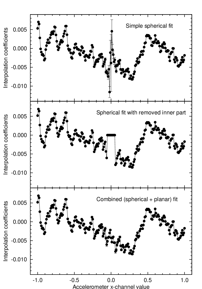
As it was noted earlier in this section, points with small $x$ , $y$ or $z$ values could cause trouble since the square of these values yields only a small increment in the value of $x^{2}+y^{2}+z^{2}$ . Indeed, the upper panel of Fig. 7 shows that the conditions used in our regression (i.e. $N=10,000$ , $N_{\rm inter}=100$ and a typical white noise of $2\cdot 10^{-4}$ ) results in an interpolation function that is “unstable” around $|x|,|y|,|z|\lesssim D_{0}=0.05$ . Therefore, we should add additional constraints to the whole procedure in order to have a reliable fit in the complete $(x,y,z)\in[-1,1]$ domain. In the following, we describe a possible method for such a reconstruction.

III.2. Planar constraints

As it was concluded at the end of Sec. III.1, that pure spherical constraints are inadequate for the calibration of the accelerometer in the domain of $|x|,|y|,|z|\lesssim D_{0}$ . It can easily be seen that the portion of the spherical surface that is affected by this effect is roughly $3D_{0}=15\%$ in total. This is a quite large area that cannot be neglected.

III.2.1 A device for planar mapping

In order to resolve this problem, we designed and built an additional calibration device that aids the calibration on this domain. This device has a single, nearly horizontal shaft on which the accelerometer itself is mounted. This horizontal axis is rotated in small steps and the accelerometer channels are read accordingly. The accelerometer has a specific attitude with respect to this horizontal shaft. During rotation, the output vectors form a circle which deflects roughly equally from all of the three axes. In other words, the normal vector of this circle is close to $(\pm 1/\sqrt{3},\pm 1/\sqrt{3},\pm 1/\sqrt{3})$ . It can easily be considered that there are four possible attitudes of the accelerometer unit with respect to the shaft that yields such a configuration in the resulting circles. Fig. 6 displays these four circles (as well as the domain on which the purely spherical constraints described earlier are viable). It can also be recognized that if one of the axes, for instance, the values of $x$ -channel are close to zero, then the other two axes have a value of $\approx\pm 1/\sqrt{2}$ . Since the intersection of a spherical surface and a plane always produce a circle, the constraint that is created by this single shaft device can be coined as a planar constraint.

Our device that performs this rotation around a single, nearly horizontal shaft is exhibited on the right panel of Fig. 5. Similarly to the four-geared mechanism, this device also features a hollow shaft driven by a timing pulley. Hence, wiring is quite easy in this case as well. At the center of the shaft, a special polyhedral structure is installed. The role of this part is to simply attach even more (currently, up to four) accelerometer units and to attain the previously noted four possible attitudes without too much effort.

As we will see later on it is not essential to have a perfectly horizontal shaft around which the accelerometer is rotated. However, the angle between the vertical and this axis must not alter during a measurement cycle. This stability is needed only during a single run: while swapping between the four possible attitudes, one can alter the attitude of the shaft with respect to the vertical as well.

III.2.2 Regression functions

As it was noted earlier, the circle measured by the accelerometer (during the rotation of the horizontal axis) is the intersection of the sphere and an appropriate plane. This plane can be characterized by the equation

n_{x}x+n_{y}y+n_{z}z=C.

(13)

This equation has four parameters: the three components of the plane normal $(n_{x},n_{y},n_{z})$ as well as the constant $C$ . However, this equation is homogeneous: the implied ambiguity between these four parameters can be resolved by applying the constraint

n_{x}^{2}+n_{y}^{2}+n_{z}^{2}=1.

(14)

In other words, the normal vector $(n_{x},n_{y},n_{z})$ should have unity length. As it was discussed above, the single shaft device maps these planes to be

|n_{x}|,|n_{y}|,|n_{z}|\approx 1/\sqrt{3}.

(15)

If Eq. (14) is satisfied, $C$ is going to be the cosine of the angle between the shaft and the vertical. The radius of the circle (i.e. the intersection of the unit sphere and this plane) is then $\sqrt{1-C^{2}}$ .

The calibration procedure, i.e. the reconstruction of the $C^{(\cdot)}_{m}$ constants for $|m|\leq D_{0}/\Delta$ is performed as follows.

First, using the points for which $D_{0}/\Delta<|m|$ , we de-trend the accelerometer outputs using the previously obtained affine coefficients followed by the interpolation procedure. These points are the parts of the red circles in Fig. 6 that lie on the yellow filled octants.

Second, these de-trended points are then substituted into Eq. (13) and by employing a least-squares fit and the additional constraint defined by Eq. (14), the values of $n_{x}$ , $n_{y}$ , $n_{z}$ and $C$ are computed. We note here that the aforementioned stability of the angle between the rotation axis and the vertical (see also at the end of Sec. III.2.1) can easily be quantified by the residual of this fit. If this fit yields a residual that is significantly larger than the residual obtained during the fit of the piecewise linear interpolation coefficients in the domain of $D_{0}/\Delta<|m|$ , then the respective measurement has to be repeated.

In the final, third step, the constants $C^{(\cdot)}_{m}$ where $|m|\leq D_{0}/\Delta$ are fitted via a simple linear least squares manner by minimizing the merit function

$\displaystyle\chi^{2}$	$\displaystyle=$	$\displaystyle\sum\limits_{\|x\|\leq D_{0}}\left[(n_{x}x^{\prime}+n_{y}y^{\prime}+n_{z}z^{\prime})-C\right]^{2}+$	(16)
		$\displaystyle\sum\limits_{\|y\|\leq D_{0}}\left[(n_{x}x^{\prime}+n_{y}y^{\prime}+n_{z}z^{\prime})-C\right]^{2}+$
		$\displaystyle\sum\limits_{\|z\|\leq D_{0}}\left[(n_{x}x^{\prime}+n_{y}y^{\prime}+n_{z}z^{\prime})-C\right]^{2}.$

where the values for $x^{\prime}$ , $y^{\prime}$ and $z^{\prime}$ are given by Eqs. (8), (9) and (10), respectively. By cause of Eq. (15) and $D_{0}\lesssim 0.05$ , the three conditions appearing in the summations of Eq. (16) are disjoint.

As it can be seen in the lower panel of Fig. 7, this procedure is capable to provide reliable values for the domains where $|x|$ , $|y|$ or $|z|$ are smaller than this limit of $D_{0}$ . The practical choice for $D_{0}$ depends on the actual $S/N$ values for the detector, the number of points sampled in the sphere and the number of points sampled in these planes/circles.

By combining the aforementioned two methods, i.e. spherical and planar constraints, the RMS residual from the perfect unit sphere is going to be in the range of $2.3\dots 2.6\times 10^{-4}$ for our accelerometer sensor units. This residual is equivalent to $0.013\dots 0.015^{\circ}\approx 0.8\dots 0.9^{\prime}\approx 48\dots 54^{\prime\prime}$ . This is only slightly larger than the white noise component of the individual components, meaning that the calibration procedure yields an accuracy comparable to the random noise.

III.3. External environment

In the following, we discuss how the foregoing procedures depend on the external environment. We focus on the effects of variations in the ambient temperature and the local gravity of the place where the calibration procedure takes place.

III.3.1 Ambient temperature

Accelerometers are also sensitive to the variations in the ambient temperature. This is an intrinsic property of the capacitive moving part of the sensor system, and not only resulted by the semiconductors of the integrated electronics, see also [5]. As we introduced earlier, our accelerometer units incorporate two precise digital thermometers mounted close to the MEMS chips. The two thermometers are mounted right above and below the accelerometer detector in a symmetric arrangement. Therefore, polling these sensors can provide reliable information not only about the accelerometer temperature but the thermal gradient in its vicinity.

Throughout the calibration procedure in our experiments, the ambient temperature was not controlled actively but the environment was quite settled. During the $\approx 4$ hours of this procedure, the measured temperature was $22.86\pm 0.16^{\circ}{\rm C}$ (RMS) while the gradient between the two thermometers was $-0.11\pm 0.02^{\circ}{\rm C}$ (RMS). Based on the datasheets, this difference is definitely smaller than the accuracy of each sensor (which is actually $0.3^{\circ}{\rm C}$ ), therefore we can safely consider isothermal conditions within the sensor package. All of the values (residuals, plots, etc.) presented earlier in this section were based on the measurements acquired in such circumstances.

Subsequently, the spherical constraint measurements has been repeated for $N=1{,}000$ points in a colder environment, namely $8.88\pm 0.14^{\circ}{\rm C}$ . This is a slight ( $\Delta T=-13.98^{\circ}{\rm C}$ ) but significant difference in the ambient temperature. If the data series from this colder measurements are de-trended using the best-fit data based on the warmer series (see earlier), the residual from the perfect sphere goes up to $\approx 0.0019$ . This RMS value implies a thermal dependence of $\approx 13\times 10^{-5}/{\rm K}$ in the accelerometer channel outputs. Using this de-trended series, we applied the procedure described in Sec. III.1.2. This affine fit yielded a residual of $0.00021$ which is in the range of the residual after the interpolation-based regression in the case of the warm data series.

Hence, we can conclude that the thermal dependence of the accelerometer outputs can be obtained in two steps. First, one applies a full (affine, spherical interpolation and planar interpolation) fit for a certain ambient temperature $T_{0}$ . Then, using these fit parameters, spherical measurements gathered on a different ambient temperature $T_{c}$ are de-trended and this output are fitted again but only for the affine coefficients. Let us denote these affine coefficients by $\Delta\hat{x}$ , $\Delta\hat{y}$ , $\Delta\hat{z}$ , $\hat{A}_{xx}$ , $\hat{A}_{yy}$ , …. If the raw values $(x,y,z)$ are read at temperature $T$ , then in first step we apply Eqs. (3), (8), (9) and (10) using the coefficients obtained at $T_{0}$ . Next, in the second step we apply Eq. (3) using the affine coefficients $k\Delta\hat{x}$ , $k\Delta\hat{y}$ , $k\Delta\hat{z}$ , $k\hat{A}_{xx}$ , $k\hat{A}_{yy}$ , …. Here $\Delta\hat{x}$ , $\Delta\hat{y}$ , etc. are obtained at the ambient temperature $T_{c}$ (see above) and

k=\frac{T-T_{0}}{T_{c}-T_{0}}.

(17)

This linear temperature dependence can be characterized more accurately by taking further measurements on various other ambient temperatures and/or by increasing the difference between $T_{0}$ and $T_{c}$ . However, such a linear approximation can be feasible on even larger temperature ranges [5, see e.g.].

III.3.2 Electronic interfaces

The responses of analog circuits (including MEMS accelerometers) depend on the voltage levels – most prominently, the power supply – applied to these electronics. In order to ensure the stability and accuracy of the whole sensor system, the supply voltage of the sensor should also be stabilized. For this purpose, we employed an onboard linear regulator that provides the nominal $+3.3\,{\rm V}$ supply of the sensor and this voltage is derived from the bus power. Such linear regulators safely reduce the relatively large variations that are allowed by, e.g. the USB standard (where it is $5.00\pm 0.25\,{\rm V}$ ). In addition, care must be taken in order to remove high-frequency components appearing on the bus(es). Hence, bypass capacitors are included in both the bus side ( $+5\,{\rm V}$ ) and sensor side ( $+3.3\,{\rm V}$ ) of the circuit.

III.3.3 Local gravity

If the local gravity changes throughout the calibration procedure, then the assumption of Eq. (2) won’t be true anymore. The relative change of the local gravity depends on the location of the Earth (i.e. the gravity itself is larger at the poles and smaller close to the equator) as well as it depends on the altitude. The altitude dependence of $g_{0}$ can be characterized as

\frac{\Delta g_{0}}{g_{0}}=-\frac{2\Delta h}{R_{0}},\vskip 0.0pt

(18)

where $\Delta h$ is the change in the altitude and $R_{0}$ is the radius of the Earth. For instance, going up by $100\,{\rm m}$ yields a decrease of $\Delta g_{0}/g_{0}\approx-3\cdot 10^{-5}$ while going north by $100\,{\rm km}$ yields an increase of $\Delta g_{0}/g_{0}\approx+5\cdot 10^{-5}$ on average, due to the oblate shape of the Earth. Furthermore, the RMS residual from the reference ellipsoid is in the range of $\sigma(\Delta g_{0}/g_{0})\approx 2\cdot 10^{-5}$ . The magnitude of these effects are bit smaller but comparable to the residual of the accelerometer calibration procedure (see above at the end of Sec. III.2). Consequently, such effects must be taken into account during the relocation of a calibrated device.

IV. Pointing models

As we emphasized in the introduction, static accelerometers are not sensitive for rotation around the vertical axis as well as these do not sense displacements. The information provided by a single static accelerometer is a vector with unity length, i.e. a point on the surface of a sphere.

In order to examine various properties of the accelerometer units while these are act as a telescope pointing sensor, we installed two units to the Schmidt telescope of the Konkoly Observatory, located at the Piszkéstető Mountain station. One of the accelerometers is mounted on the fork of the telescope (see also Fig. 1 a) while the other one is mounted on the side of the telescope tube (Fig. 1 b). Both accelerometers are fixed in a kind of arbitrary attitude, the only constraint is that the $z+$ axis of the first unit sensor (#1, mounted on the fork) is roughly parallel with the hour axis and points towards north while the $z+$ axis of the second sensor (#2) is more-or-less perpendicular to the optical axis. For this setup, we used a USB-RS485 converter as a bus master which is connected to unit #1, followed by unit #2. The termination resistors of the bus are placed after unit #2.

In this section, we investigate how can one derive the output of these accelerometers. The following series of computations does not depend on our actual setup, it can simply be adopted to any equatorial telescope mount.

IV.1. Using the accelerometer as an attitude sensor

Let us suppose that an ideal static accelerometer is placed horizontally. In this case, its output vector is $\mathbf{a}=(x,y,z)=(0,0,g_{0})$ , where $g_{0}$ is magnitude of the local gravity. It can be considered that if the active transformation $\mathbf{R}$ is applied on the accelerometer package, then the sensed vector is

\mathbf{a}=-\mathbf{g}\cdot\mathbf{R}.

(19)

Here $\mathbf{g}=(0,0,-g_{0})$ is the gravitational acceleration vector in the static (external) reference frame defined by the $\mathbf{x}_{0}$ , $\mathbf{y}_{0}$ and $\mathbf{z}_{0}$ axes. The active nature of the transformation means the following. Let us denote the reference frame fixed to the accelerometer package by the $\mathbf{x}$ , $\mathbf{y}$ and $\mathbf{z}$ axes. Using these notations, the active transformation means that

$\displaystyle\mathbf{x}$	$\displaystyle=$	$\displaystyle\mathbf{R}\cdot\mathbf{x}_{0},$	(20)
$\displaystyle\mathbf{y}$	$\displaystyle=$	$\displaystyle\mathbf{R}\cdot\mathbf{y}_{0},$	(21)
$\displaystyle\mathbf{z}$	$\displaystyle=$	$\displaystyle\mathbf{R}\cdot\mathbf{z}_{0}.$	(22)

In Fig. 8 we display the definitions of these vectors. In the following, we expect that the calibration procedure described in Sec. III has carefully been performed, thus the accelerometer output can be interpreted (within the accuracy of the calibration fit RMS) as an output of an ideal accelerometer. One must note that the accelerometer output vector is computed as a post-multiplication of the vector $-\mathbf{g}$ by the active rotation matrix $\mathbf{R}$ . If $g_{0}$ is unity, then the components of the output vector $\mathbf{a}=(a_{1},a_{2},a_{3})\equiv(x^{\prime\prime},y^{\prime\prime},z^{\prime\prime})$ are $a_{1}=R_{31}$ , $a_{2}=R_{32}$ and $a_{3}=R_{33}$ . Alternatively, one can use the form

\mathbf{a}=\mathbf{R}^{\rm T}\cdot(-\mathbf{g}),

(23)

where $(\cdot)^{\rm T}$ denotes matrix transposition.

In the following, we investigate how the matrix $\mathbf{R}$ is computed if the telescope parameters (most notably, the geographic latitude) and the position of the axes are known.

IV.2. A simple isotropic pointing model

As it was introduced above, the current goal is to compute the transformation $\mathbf{R}$ that actively transform the accelerometer from its “rest” position into the actual point where the telescope points. Now we consider only an accelerometer that is mounted on the telescope tube (referred as #2 earlier above) since the role of the other one on the hour axis is less crucial and the related computation is much simpler. Assuming an ideal construction, this matrix of $\mathbf{R}$ is computed as

\mathbf{R}=\mathbf{G}\cdot(\mathbf{P}_{\rm t}\cdot\mathbf{P}_{\rm d})\cdot\mathbf{A}.

(24)

Here, $\mathbf{A}$ is the transformation that “glues” the accelerometer chip to the tube, $\mathbf{P}_{\rm d}$ and $\mathbf{P}_{\rm t}$ are the transformations that rotates the telescope axes (declination and hour axis, respectively) and $\mathbf{G}$ what “installs” the telescope hour axis to its proper place on the ground. If we denote the actual hour angle and declination values by $\tau$ and $\delta$ , respectively while the geographic longitude is $\varphi$ , then these matrices are written as

$\displaystyle\mathbf{G}$	$\displaystyle=$	$\displaystyle\begin{pmatrix}\sin\varphi&0&-\cos\varphi\\ 0&1&0\\ \cos\varphi&0&\sin\varphi\end{pmatrix},$	(25)
$\displaystyle\mathbf{P}_{\rm t}$	$\displaystyle=$	$\displaystyle\begin{pmatrix}\cos\tau&\sin\tau&0\\ -\sin\tau&\cos\tau&0\\ 0&0&1\end{pmatrix},$	(26)
$\displaystyle\mathbf{P}_{\rm d}$	$\displaystyle=$	$\displaystyle\begin{pmatrix}\cos\delta&0&-\sin\delta\\ 0&1&0\\ \sin\delta&0&\cos\delta\end{pmatrix},$	(27)

while $\mathbf{A}$ depends on how we mounted the sensor to the tube. Throughout these computations, the reference axes $\mathbf{x}_{0}$ , $\mathbf{y}_{0}$ and $\mathbf{z}_{0}$ point towards south, east and to the zenith, respectively – and hence form a right-hand coordinate system. In the case of an improper, but still isotropic alignment of the telescope, the product $\mathbf{P}:=\mathbf{P}_{\rm t}\cdot\mathbf{P}_{\rm d}$ is written in the form

\mathbf{P}=\mathbf{H}\cdot\mathbf{P}_{\rm t}\cdot\mathbf{X}\cdot\mathbf{P}_{\rm d}\cdot\mathbf{T}.

(28)

Here the matrices $\mathbf{H}$ , $\mathbf{X}$ and $\mathbf{T}$ encodes the various misalignments, including polar misalignment, encoder zero points, cross axis deflection, optical axis misalignment [see e.g. 19, for a more detailed description of these deviations]. Ideally, all of transformations $\mathbf{H}$ , $\mathbf{X}$ and $\mathbf{T}$ are unity. If these deflections are small, then a first-order expansion can be applied using the exponential form of ${\rm SO}(3)$ transformations:

$\displaystyle\mathbf{H}$	$\displaystyle=$	$\displaystyle\exp\begin{pmatrix}0&-c&b\\ c&0&-a\\ -b&a&0\end{pmatrix}\approx\begin{pmatrix}1&-c&b\\ c&1&-a\\ -b&a&1\end{pmatrix}$	(29)
$\displaystyle\mathbf{X}$	$\displaystyle=$	$\displaystyle\exp\begin{pmatrix}0&-f&e\\ f&0&-d\\ -e&d&0\end{pmatrix}\approx\begin{pmatrix}1&-f&e\\ f&1&-d\\ -e&d&1\end{pmatrix}$	(30)
$\displaystyle\mathbf{T}$	$\displaystyle=$	$\displaystyle\exp\begin{pmatrix}0&-i&h\\ i&0&-g\\ -h&g&0\end{pmatrix}\approx\begin{pmatrix}1&-i&h\\ g&1&-g\\ -h&g&1\end{pmatrix}$	(31)

For our purposes, “small” means that the second-order terms are negligible compared to the pointing residual $\sigma_{\rm pointing}$ . This is limited now by the accuracy of the accelerometers, i.e. $\sigma_{\rm pointing}\approx\sigma_{\rm accelerometer}$ . In other words, this condition is equivalent to

a^{2}+b^{2}+c^{2},d^{2}+e^{2}+f^{2},g^{2}+h^{2}+i^{2}\lesssim\sigma_{\rm pointing}.

(32)

It can be shown that the first-order series expansion of Eq. (28) depends only on the sums $c^{\prime}:=c+f$ and $e^{\prime}:=e+h$ . For completeness, here we give the full expansion of this equation up to the first order. In the formula presented below, $c_{\rm t}$ , $s_{\rm t}$ , $c_{\rm d}$ and $s_{\rm d}$ denotes $\cos\tau$ , $\sin\tau$ , $\cos\delta$ and $\sin\delta$ , respectively:

$\displaystyle\mathbf{P}$	$\displaystyle\approx$	$\displaystyle\begin{pmatrix}c_{\rm t}c_{\rm d}&s_{\rm t}&-c_{\rm t}s_{\rm d}\\ -s_{\rm t}c_{\rm d}&c_{\rm t}&s_{\rm t}s_{\rm d}\\ s_{\rm d}&0&c_{\rm d}\end{pmatrix}+a\begin{pmatrix}0&0&0\\ -s_{\rm d}&0&-c_{\rm d}\\ -s_{\rm t}c_{\rm d}&c_{\rm t}&s_{\rm t}s_{\rm d}\end{pmatrix}$	(33)
		$\displaystyle+b\begin{pmatrix}s_{\rm d}&0&c_{\rm d}\\ 0&0&0\\ -c_{\rm t}c_{\rm d}&-s_{\rm t}&c_{\rm t}s_{\rm d}\end{pmatrix}+c^{\prime}\begin{pmatrix}s_{\rm t}c_{\rm d}&-c_{\rm t}&-s_{\rm t}s_{\rm d}\\ c_{\rm t}c_{\rm d}&s_{\rm t}&-c_{\rm t}s_{\rm d}\\ 0&0&0\end{pmatrix}+$
		$\displaystyle+d\begin{pmatrix}-s_{\rm t}s_{\rm d}&0&-s_{\rm t}c_{\rm d}\\ -c_{\rm t}s_{\rm d}&0&-c_{\rm t}c_{\rm d}\\ 0&1&0\end{pmatrix}+e^{\prime}\begin{pmatrix}c_{\rm t}s_{\rm d}&0&c_{\rm t}c_{\rm d}\\ -s_{\rm t}s_{\rm d}&0&-s_{\rm t}c_{\rm d}\\ -c_{\rm d}&0&s_{\rm d}\end{pmatrix}+$
		$\displaystyle+g\begin{pmatrix}0&-c_{\rm t}s_{\rm d}&-s_{\rm t}\\ 0&s_{\rm t}s_{\rm d}&-c_{\rm t}\\ 0&c_{\rm d}&0\end{pmatrix}+i\begin{pmatrix}s_{\rm t}&-c_{\rm t}c_{\rm d}&0\\ c_{\rm t}&s_{\rm t}c_{\rm d}&0\\ 0&-s_{\rm d}&0\end{pmatrix}.$

If the transformation $\mathbf{A}$ is not accurately known, then the respective corrections will appear in $\mathbf{T}$ via the parameters $g$ , $e^{\prime}=e+h$ and $i$ . This is due to the fact that in the final form of transformation Eq. (24), only the product $\mathbf{T}\cdot\mathbf{A}$ appears. In the following, we proceed with the determination of the pointing model parameters ( $a$ , $b$ , $c^{\prime}$ , …).

IV.3. Attitude calibration

In order to evaluate Eq. (19), we have to know not only the pointing parameters and transformations but the accelerometer attitude $\mathbf{A}$ with respect to the telescope tube. As we noted earlier, in our experiment we mounted the tube unit in a somehow random attitude due to the limited mounting possibilities (see Fig. 1 b). However, the corresponding transformation can easily be estimated by combining some rotations whose product yields the desired attitude. Our findings for this attitude was

\mathbf{A}=\begin{pmatrix}+0.6307&-0.7759&-0.0135\\ -0.3365&-0.2577&-0.9057\\ +0.6993&+0.5758&-0.4237\end{pmatrix}.

(34)

Before comparing the expected accelerometer outputs with the measured ones, we have to multiply Eq. (33) by $-\mathbf{g}\cdot\mathbf{G}$ from the left and by $\mathbf{A}$ from the right. However, it is easier to multiply the accelerometer outputs $\mathbf{a}$ by the transpose (inverse) of $\mathbf{A}$ , thus our constraint will be the relation

-\mathbf{g}\cdot\mathbf{G}\cdot(\mathbf{P})=\mathbf{a}\cdot\mathbf{A}^{\rm T}.

(35)

If a series of $\mathbf{a}_{k}$ values are given with the corresponding $\tau_{k}$ , $\delta_{k}$ values, one should minimize the merit function

\chi^{2}=\sum_{k}\left(-\mathbf{g}\cdot\mathbf{G}\cdot\mathbf{P}_{k}-\mathbf{a}_{k}\cdot\mathbf{A}^{\rm T}\right)^{2}

(36)

in order to find the best-fit values of the pointing model parameters $a$ , $b$ , $c^{\prime}$ , $d$ , etc. Since $\mathbf{g}=(0,0,-1)$ (considering unity local gravitational acceleration), the components of the vector $-\mathbf{g}\cdot\mathbf{G}$ are going to be

-\mathbf{g}\cdot\mathbf{G}=\begin{pmatrix}\cos\varphi\\ 0\\ \sin\varphi\end{pmatrix}.

(37)

By multiplying Eq. (33) with this vector from the left, we got the expansion

	$\displaystyle-\mathbf{g}\cdot\mathbf{G}\cdot\mathbf{P}=\begin{pmatrix}c_{\rm p}c_{\rm t}c_{\rm d}+s_{\rm p}s_{\rm d}\\ c_{\rm p}s_{\rm t}\\ -c_{\rm p}c_{\rm t}s_{\rm d}+s_{\rm p}c_{\rm d}\end{pmatrix}+a\begin{pmatrix}-s_{\rm p}s_{\rm t}c_{\rm d}\\ s_{\rm p}c_{\rm t}\\ s_{\rm p}s_{\rm t}s_{\rm d}\end{pmatrix}+$		(38)
	$\displaystyle+b\begin{pmatrix}c_{\rm p}s_{\rm d}-s_{\rm p}c_{\rm t}c_{\rm d}\\ -s_{\rm p}s_{\rm t}\\ c_{\rm p}c_{\rm d}+s_{\rm p}c_{\rm t}s_{\rm d}\end{pmatrix}+c^{\prime}\begin{pmatrix}c_{\rm p}s_{\rm t}c_{\rm d}\\ -c_{\rm p}c_{\rm t}\\ -c_{\rm p}s_{\rm t}s_{\rm d}\end{pmatrix}+d\begin{pmatrix}-c_{\rm p}s_{\rm t}s_{\rm d}\\ s_{\rm p}\\ -c_{\rm p}s_{\rm t}c_{\rm d}\end{pmatrix}+$
	$\displaystyle+e^{\prime}\begin{pmatrix}c_{\rm p}c_{\rm t}s_{\rm d}-s_{\rm p}c_{\rm d}\\ 0\\ c_{\rm p}c_{\rm t}c_{\rm d}+s_{\rm p}s_{\rm d}\end{pmatrix}+g\begin{pmatrix}0\\ -c_{\rm p}c_{\rm t}s_{\rm d}+s_{\rm p}c_{\rm d}\\ -c_{\rm p}s_{\rm t}\end{pmatrix}+$
	$\displaystyle+i\begin{pmatrix}c_{\rm p}s_{\rm t}\\ -c_{\rm p}c_{\rm t}c_{\rm d}-s_{\rm p}s_{\rm d}\\ 0\end{pmatrix}.$

Here $c_{\rm p}=\cos\varphi$ and $s_{\rm p}=\sin\varphi$ . It can be computed that the three vectors whose coefficients are $a$ , $b$ and $c^{\prime}$ are linearly dependent for arbitrary values of $\varphi$ , $\tau$ and $\delta$ . This property is implied by the fact that the accelerometer output is invariant for the rotations around the $\mathbf{z}_{0}\pm$ axis. Due to the several subsequently applied transformations needed to compute the final $\mathbf{a}$ vector, this invariance is not obvious at the first glance and appears indirectly via this lost of linear independence. All of the other vectors appearing in the equation above are independent in this sense. For simplicity, in the following we cancel the term corresponding to $c^{\prime}$ .

Now it is straightforward to perform the minimization of Eq. (36). In order to test the above computations and hence estimate the real-life accuracy of the sensors, we took 23 images by the Schmidt telescope to gather sufficient (and unbiased) information about the pointing of the accelerometers. The basic steps of image reduction are performed with the FITSH package [16] while astrometry is performed both by this package [using the USNO-B catalog of 13, as reference] and the online version of the Astrometry.net project [11]. The corresponding values for the hour angle ( $\tau$ ) and declination ( $\delta$ ) that are needed in the expansion of Eq. (38) could be taken from both by the astrometric solutions and from the rotary encoders mounted inside the driving mechanisms of the telescope mount. First, J2000 centroids must be converted to first equatorial system for the epoch of image acquisition (by taking into account precession, nutation, aberration and refraction). For this purpose, we involved the algorithms provided by [15]. The linear regression is performed by using the algorithms of [18] and the implementation provided by the FITSH utility lfit [16]. The results of the fit are

$\displaystyle a$	$\displaystyle=$	$\displaystyle-0.00091\pm 0.00017$	(39)
$\displaystyle b$	$\displaystyle=$	$\displaystyle+0.00019\pm 0.00010$	(40)
$\displaystyle d$	$\displaystyle=$	$\displaystyle-0.00011\pm 0.00021$	(41)
$\displaystyle e^{\prime}$	$\displaystyle=$	$\displaystyle+0.00975\pm 0.00011$	(42)
$\displaystyle g$	$\displaystyle=$	$\displaystyle+0.00082\pm 0.00013$	(43)
$\displaystyle i$	$\displaystyle=$	$\displaystyle-0.00070\pm 0.00025,$	(44)

while the fit residual is $0.00025$ . This value is equivalent to $0.0143^{\circ}=0.86^{\prime}=52^{\prime\prime}$ . Therefore, we can safely conclude that accelerometers provide the sub-arcminute accuracy as the part of a real TCS. In addition, the timespan between the calibration of the sensors and this attitude fit was approximately two months. We note, there are other noise sources that are present in accelerometer systems and not quantified by any of our calibration steps. These include the effect of mechanical vibrations of the telescope system as well as the Allan variance presented in the output of MEMS accelerometers. However, the gross yield of these are also included in the final fit residual. The magnitude of long-term systematic variations can be characterized by repeating the attitude calibration over longer timespan. In addition, the telescope itself can be utilized as a two-axis device in order to estimate other sources for the temporal variations in, at least, the affine part of the calibration procedure.

IV.4. Extraction of pointing information

Expecting an accelerometer to be the primary absolute pointing encoder of a telescope system, one can be curious how the pointing (i.e. the $\tau$ and $\delta$ angles) can be recovered from the accelerometer outputs. In Fig. 9 we plotted the contour lines (more specifically, the isolines) of an equatorial telescope located on the temperate geographical latitude $\varphi=47.5^{\circ}$ . In these plots, the attitude $\mathbf{A}$ of the accelerometer with respect to the telescope is the same what it was in our experiments (see Eq. 34). The topology of the contour lines shows the ambiguity of the accelerometer outputs: there are positions corresponding to different $(\tau,\delta)$ values which yield the similar $\mathbf{a}$ output. However, it can be considered that this ambiguity is bimodal and can safely be resolved once the value of $\tau$ is known. Therefore, an accelerometer-based TCS should employ two such units: one is mounted on the polar axis while the other one is fixed to the tube itself – and even a rough value for the $\tau$ is sufficient to resolve the bimodality.

In practice, one has to invert Eq. (35) by substituting the expression of Eq. (38) where the latter one is a function of $\tau$ and $\delta$ . Due to the first-order expansion, it can be performed in an iterative way. First, one solve the equation

\begin{pmatrix}\cos\varphi\cos\tau\cos\delta+\sin\varphi\sin\delta\\ \cos\varphi\sin\tau\\ -\cos\varphi\cos\tau\sin\delta+\sin\varphi\cos\delta\end{pmatrix}=\begin{pmatrix}a_{x}\\ a_{y}\\ a_{z}\end{pmatrix},

(45)

for $(\tau,\delta)$ where $(a_{x},a_{y},a_{z})$ are the components of the product $\mathbf{a}\cdot\mathbf{A}^{\rm T}$ . Then, the solution is substituted to the first-order terms (proportional to $a$ , $b$ , $d$ , …) and subtracted from $(a_{x},a_{y},a_{z})$ and the iteration is repeated until convergence. The solution of the above equation is going to be

	$\displaystyle\tau$	$\displaystyle=$	$\displaystyle 90^{\circ}\pm\mathrm{arc\,cos}\left(\frac{a_{y}}{\cos\varphi}\right),$		(46)
	$\displaystyle\delta$	$\displaystyle=$	$\displaystyle\mathrm{arg}\left(d_{x},d_{y}\right),$		(47)

where

	$\displaystyle d_{x}$	$\displaystyle=$	$\displaystyle a_{x}\cos\varphi\cos\tau+a_{z}\sin\varphi,$		(48)
	$\displaystyle d_{y}$	$\displaystyle=$	$\displaystyle a_{x}\sin\varphi-a_{z}\cos\varphi\cos\tau.$		(49)

The bimodality in the hour angle, i.e. the sign in Eq. (46) can safely be figured out by using a secondary accelerometer. Once $\tau$ is known accurately, the value for $\delta$ is unambiguous.

The characteristics of the isolines in Fig. 9 are also prominent. Naively, one can expect that due to the limits implied by the local horizon, only the half of the sphere is covered by accelerometer. However, due to the finite angle between the horizon and the primary axis of the telescope, further information is lost: only a stripe in the sphere is covered (which is also cut in half due to the horizon). The area of this partial stripe relative to the total surface is $\cos\varphi/2$ . The northern or southern the telescope location, the smaller the covered area. In the poles, equatorial mounts behave similarly as alt-azimuthal mounts and hence accelerometers could not provide sufficient information for the pointing attitude.

Exploiting the relation for horizontal altitude $h$ , it can be computed rather elegantly, viz.

\sin h=a_{x}.

(50)

The above equation shows how accelerometer outputs can be interpreted if this sensor is used as a horizontal limit switch. We note here, however, that fast slewing and the implied centrifugal acceleration distort the output and it must therefore be quantified before such an application. The magnitude of this distortion depends on both the slewing speed and the displacement of the sensors from the axes. Considering a normal slewing speed of two degrees per second (i.e. $0.03\,{\rm rad}/{\rm s}$ ) and characteristic instrument size of a few meters, this centrifugal acceleration is going to be in the range of $\lesssim 10^{-3}\,g$ , which is equivalent to few arcminutes.

V. Summary

In this paper we demonstrated how cheap MEMS accelerometers can accurately be calibrated and involved as a part of a telescope control system. Our main conclusion can be summarized in a single number, namely the fit residual of the telescope pointing fit procedure. This value shows us that the sub-arcminute RMS accuracy can safely be targeted. This accuracy includes the accuracy of the standalone calibration, the compensation of effects due to the variations in the ambient temperature as well as the compensation of telescope mount deflections.

Considering the techniques of the implementation, exploiting such sensors needs no changes in the existing electromechanical components of a telescope system at all. The sensors are simply mounted on the respective mechanisms (hour axis and tube) and the actual attitude of the mounting is also irrelevant. This is a great advantage over the electromechanical feedback systems widely employed in TCSs. In addition, the $2\times 3$ channels are redundant and very sensitive of unintentional tampering of these devices. This property further increases the reliability of an autonomous and/or remotely operated observatory.

One of the further goals of ours is to exploit such an accurately calibrated set of accelerometers in unconventional mechanics like hexapods [3, 10, 17]. In this case, accelerometers can be mounted onto the base and payload platform as well as on all of the six, topologically identical legs. The information provided by the $8\times 3$ accelerometer channels can be sufficient and redundant to recover the attitude and displacement (i.e. 6 degrees of freedom) of the payload with respect to the base. Our findings for the accuracy is comparable to the per-pixel resolution of wide-field hexapod-based instruments [17, 20]. Hence, such systems might benefit even more than high resolution instrumentation.

This research is conducted as a part of the “Fly’s Eye” project which is supported by the Hungarian Academy of Sciences via the grant LP2012-31. Additional support is also received via the OTKA grants K-109276 and K-104607. We thank F. Schlaffer for aiding the fabrication of the accelerometer enclosures. We also thank the help and quick responses of our colleagues, R. Szakáts, K. Vida, Gy. Mező, M. Rácz, L. Molnár and L. Döbrentei during the installation and calibration of the sensors. We also thank the valuable comments and suggestions of the anonymous referee. In our project, we involved numerous free & open source software, including gEDA (for schematics and PCB design), OpenSCAD (3D parametric designs), FreeCAD (3D designs), CURA (3D slicing, GCODE generation and printing control) and AVR-GCC (for MCU programming).

References

[1] Buie, M.: General Analytical Telescope Pointing Model, available from http://www.boulder.swri.edu/˜buie/idl/ /downloads/pointing/pointing.pdf
[2] Burd, A. et al. 2005, New Astron., 10, 409
[3] Chini, R. 2000, Rev. Mod. Astron., 13, 257
[4] Chollet, F. & Liu, H.-B.: A (not so) short Introduction to Micro Electromechanical Systems, v. 5.1, 2013, available from http://memscyclopedia.org/
[5] Dai, G. et al. 2010, Proceedings of the 5th IEEE International Conference on Nano/Micro Engineered and Molecular Systems, p. 82
[6] Fors, O. et al. 2013, PASP, 125, 522
[7] Granzer, T. et al. 2012, Astron. Nachtr., 333, 823
[8] Hirt, Ch. 2006, A&A, 459, 283
[9] Hirt, Ch. & Seeber, G. 2008, J. Geodesy, 82, 347
[10] Koch, P. M. et al. 2009, ApJ, 694, 1670
[11] Lang, D. et al. 2010, AJ, 139, 1782
[12] Lee, I. et al. 2005, Sens. Actuators A, 119, 8
[13] Monet, D. G. et al. 2003, AJ, 125, 984
[14] Maureira, E. 2014, to appear in the proceedins of Third Workshop on Robotic Autonomous Observatories, Torremolinos (Málaga), Spain
[15] Meeus, J.: Astronomical algorithms (2nd ed.), 1998, Richmond, VA: Willmann-Bell.
[16] Pál, A. 2012, MNRAS, 421, 1825
[17] Pál, A. et al. 2013, Astron. Nachtr., 334, 932
[18] Press, W. H., Teukolsky, S. A., Vetterling, W.T., Flannery, B.P., 2002, Numerical Recipes in C++: the art of scientific computing, Third Edition, Cambridge University Press
[19] Spillar, E. J. et al. 1993, PASP, 105, 616
[20] Vida, K. et al. 2014, Proceedings of “Observing techniques, instrumentation and science for metre-class telescopes”, Contributions of the Astronomical Observatory Skalnaté Pleso, 43, 530
[21] Zhang, X.-x. & Wu, L.-d. 2001, Chinese Astron. Astrophys., 25, 499