跳到论文正文
W Papers独立论文阅读器 arXiv:1407.0027 论文正文 计算阅读时间 · 0%
引用这篇论文根据当前论文元数据生成,正式投稿前建议核对。


License: arXiv.org perpetual non-exclusive license
arXiv:1407.0027v2 [hep-th] 09 Dec 2014

LMU-ASC 43/14

Towards the One-loop Kähler Metric
of Calabi-Yau Orientifolds

Marcus Berg+, Michael Haack†, Jin U Kang⋆, Stefan Sjörs♡

+ Department of Physics, Karlstad University
651 88 Karlstad, Sweden
† Arnold Sommerfeld Center for Theoretical Physics
Ludwig-Maximilians-Universität München
Theresienstrasse 37, 80333 München, Germany
⋆ Department of Physics, Kim Il Sung University
RyongNam Dong, TaeSong District, Pyongyang, DPR. Korea
and
Department of Physics, Nanjing University
22 Hankou Road, Nanjing 210093, PR. China
and
Abdus Salam International Centre for Theoretical Physics
Strada Costiera 11, Trieste 34014, Italy
♡ Institut für Theoretische Physik, Universität Heidelberg,
Philosophenweg 19, D-69120 Heidelberg

Abstract

We evaluate string one-loop contributions to the Kähler metric of closed string moduli in toroidal minimally supersymmetric (Calabi-Yau) orientifolds with D-branes. We focus on the poorly understood 𝒩=1{\mathcal{N}}=1 sectors that receive contributions from all massive string states.

1 Introduction

Orientifolds and orbifolds with D-branes (see e.g. [1, 2] for reviews) are valuable theoretical laboratories for understanding string models of phenomenological relevance. They are the simplest nontrivial string models, in the sense that the worldsheet theories are free, but the symmetry is reduced compared to the simplest possible models. At the phenomenological level, too much symmetry can prevent a given string model from accommodating existing and future data, but too little symmetry makes direct computations exceedingly difficult. For example, if we orientifold Type IIB string theory to produce Type I string theory in 10 dimensions, then compactify on an orbifold that is a limit of the six-dimensional space K​3×T2K3\times T^{2}, we are left with extended 𝒩=2{\mathcal{N}=2} supersymmetry in four dimensions. In 𝒩=2{\mathcal{N}=2} supersymmetric models it is typically relatively straightforward to compute string effective actions from worldsheet conformal field theory including the first quantum corrections, in the approximation of one string loop. This is because only zero modes contribute to the string effective actions, as heavy string states do not preserve enough supersymmetry, which effectively means that all dependence on worldsheet moduli cancels out of the integrands of string S-matrix elements, an enormous technical simplification. However, these models are not terribly attractive for phenomenology.

Instead one usually wants to compactify string theory on an orientifold that is a limit of a true Calabi-Yau manifold, to obtain minimal 𝒩=1{\mathcal{N}=1} supersymmetry in four dimensions. In these more generic models, the amount of supersymmetry is not enough to make the worldsheet conformal field theory calculations trivial. There remain integrals over both moduli of the worldsheet metric itself, and over the positions of vertex operators. (For example, for a cylinder amplitude, the worldsheet moduli are the length of the cylinder and all vertex positions. At tree level, one would fix some positions by conformal symmetry, but at one-loop this is not as helpful and vertex operators are often left unfixed.) In simple terms, there is no reason for 𝒩=1{\mathcal{N}}=1 contributions to simplify like 𝒩=2{\mathcal{N}}=2 sectors do.

On the good side, there is an extensive literature where somewhat related calculations have been performed; minimally supersymmetric string effective actions for the heterotic string from the 1980s, and some later developments. It would not be useful or feasible to cite them all here, but we wish to highlight papers by Lerche, Schellekens, Nilsson and Warner from 1987 [3] and by Stieberger and Taylor from 2002 [4]. In these papers, very impressive calculations of torus integrals are performed, where the integrands are highly nontrivial functions of both positions and worldsheet metric moduli. For orientifolds with D-branes, such calculations would need to be generalized to other worldsheet surfaces at Euler characteristic zero, with worldsheet boundaries and/or crosscaps (annulus, Möbius strip, and Klein bottle, that we collectively denote by σ\sigma). At first sight this generalization seems impossible, since important details of torus integrals were used that simply do not apply in orientifolds with D-branes.

In this paper, we will emphasize the existence of a natural mapping between gravity-like amplitudes (closed strings) and gauge-theory-like amplitudes (open and unoriented strings) at one loop. The three worldsheet surfaces σ\sigma with boundaries and crosscaps are themselves defined as involutions of a covering torus. This means that one can use the “doubling trick”, i.e. extend worldsheet fields to unphysical regions of the worldsheet surface (“unphysical” in the sense of the method of images). Including these unphysical regions reconstitutes the covering torus. It is then in principle possible to use methods similar to those of closed strings, but it is not completely trivial. For example, the alert reader will have noted that this could at most be possible for open and/or unoriented string amplitudes where certain factors (such as Chan-Paton traces) have been stripped off.

We will be interested in one-loop corrections to the Kähler metric of closed string moduli in 𝒩=1{\mathcal{N}}=1 supersymmetry. In [5] we studied the one-loop correction to the Kähler metric of open string scalars for D-branes intersecting at angles, and found that it vanishes in one special case. This is not guaranteed by supersymmetric effective field theory, and more generally, one does not expect it to vanish. In this paper we take a step back from [5] in the sense that we do not allow nontrivial intersection angles between the D-branes, or D-brane worldvolume fluxes. This means that the moduli dependence will be simple and the essential output of our calculation can be reduced to a single computable finite constant for each given model. This may be relevant for the phenomenology of these models, for example in determining the Kähler metrics for the moduli fields. We emphasized “finite” constant, since in analogous open-string calculations (e.g. [6]), there can be infrared-divergent field theory contributions that produce anomalous dimensions for the effective fields below the string scale, which introduces possibly interesting renormalization group evolution. In the current setting with closed string moduli, there are no such infrared-divergent contributions. Provided the consistency conditions from tadpole cancellation are fulfilled, ultraviolet divergences in the string amplitude of interest also cancel between the various diagrams, so there are no divergences at all.

Other work that is relevant to this general kind of calculation include [7, 8, 9]. We keep the general outline as generic as possible throughout this paper, but for concreteness we occasionally focus on a particular Kähler modulus for a particular orientifold. As example we use the Kähler modulus of the third two-torus in the ℤ6′\mathbb{Z}_{6}^{\prime} orientifold, whose orbifold generator is defined by the twist vector v→=(16,−12,13)\vec{v}=(\frac{1}{6},-\frac{1}{2},\frac{1}{3}). This minimally supersymmetric four-dimensional orientifold contains D9-branes as well as D5-branes wrapped around the third torus. Without fluxes or angles, T-duality in all six internal directions exchanges the D-brane configuration for one with D3-branes and D7-branes, respectively.

2 String effective action

The moduli space of closed and open string moduli is of great interest, both in its own right and in applications. Typically in Type IIB orientifolds, the moduli are Kähler moduli TT, complex structure moduli UU, the complexified dilaton SS, and D-brane moduli φ\varphi. After moduli stabilization such as in flux compactifications, most of these fields will be heavy and should better be called “would-be moduli”. Here, we will not incorporate any direct effects of moduli stabilization. In fact, experience shows that minimization of the effective moduli potential should be attempted after the string effective action is understood at least at the one-loop level. Perhaps surprisingly, certain questions may even require understanding of the string effective action at higher-loop level, as we argue below.

The string effective Lagrangian at low energy α′​E2≪1\alpha^{\prime}E^{2}\ll 1, in the Einstein frame, will contain the moduli metric of the Kähler moduli:

ℒeff⊃GT​T¯​∂μT​∂μT¯.\displaystyle{\mathcal{L}}_{\rm eff}\quad\supset\quad G_{T\bar{T}}\,\partial_{\mu}T\partial^{\mu}\bar{T}\;. (1)

In the following, we are going to focus on the metric for T3T_{3}, the Kähler modulus of the 3rd two-torus of the orientifold under consideration. If TT does not carry a subscript, we always implicitly mean this modulus. Before we begin, a few comments about eq. (1). We employ ‘‘moduli space power counting’’11 1 see e.g. [10], appendix B.. That is, we assign dimension zero to all classical field expectation values, as opposed to the canonical dimensions dictated by the quantum fields (fluctuations). This means we can keep all powers of e.g. TT in GT​T¯G_{T\bar{T}} without any tension with the low-energy truncation of the α′\alpha^{\prime} expansion, as long as we view the TT in GT​T¯G_{T\bar{T}} as being the classical expectation value. With this understanding, one may be misled to believe that we can always set GT​T¯→δT​T¯G_{T\bar{T}}\;\rightarrow\;\delta_{T\bar{T}} by canonically normalizing TT. The metric can indeed be transformed to the flat metric at a point, but not when we probe the neighborhood of a point. For example, the Kaplunovsky-Louis soft terms in gravity mediated supersymmetry breaking [11] involve curvature tensors in field space. In general, we would like to know the moduli space metric GT​T¯G_{T\bar{T}}, including quantum corrections.

In minimal supersymmetry, the moduli space metric GT​T¯G_{T\bar{T}} is Kähler, but it is not protected from renormalization. We remark that if we instead had considered the more symmetric models with extended 𝒩=2{\mathcal{N}}=2 supersymmetry (or more), the Kähler metric would have been given in terms of a prepotential, which is holomorphic and obeys nonrenormalization theorems analogous to those of the gauge kinetic function in minimal supersymmetry.

With enough Kähler metric components computed, one can hope to “integrate” the Kähler metric to obtain the Kähler potential from which all Kähler metric components are derived, as in [12]. We will not solve this problem in the present paper, but rather focus on a single metric component.

To compute a one-loop correction to GT​T¯G_{T\bar{T}}, we need to calculate a two-point function of closed string vertex operators representing the volume of the 3rd torus measured in the string frame. This is the objective of this paper. However, our result is not quite sufficient to construct the one-loop correction to the moduli metric of TT in the Einstein frame. We would also need to take into account the perturbative correction to the Einstein-Hilbert term. To see that this will have an influence on the moduli metric in the four-dimensional Einstein frame, let us consider the analogous 𝒩=2{\cal N}=2 supersymmetric model discussed in [13]. (To be precise, those authors only considered Kähler moduli that are transverse to the overall volume, which would not include the Kähler modulus T3T_{3} that we are considering in this paper. The following discussion is only meant to illustrate possible effects of corrections to the Einstein-Hilbert term.) To one-loop order, the corrections to the Einstein-Hilbert term and the moduli metric are found to be

S4\displaystyle S_{4} =\displaystyle= 12​κ42​∫d4​x​−g​[e−2​Φ4+χ(2​π)3​(2​ζ​(3)​e−2​Φ4𝒱+2​π23)]​R\displaystyle\frac{1}{2\kappa_{4}^{2}}\int d^{4}x\sqrt{-g}\left[e^{-2\Phi_{4}}+\frac{\chi}{(2\pi)^{3}}\left(2\zeta(3)\frac{e^{-2\Phi_{4}}}{{\cal V}}+\frac{2\pi^{2}}{3}\right)\right]R (2)
+1κ42∫d4x−g[e−2​Φ4−χ(2​π)3(2ζ(3)e−2​Φ4𝒱+2​π23)]Gq​q¯(0)∂μq∂μq¯+…,\displaystyle+\frac{1}{\kappa_{4}^{2}}\int d^{4}x\sqrt{-g}\left[e^{-2\Phi_{4}}-\frac{\chi}{(2\pi)^{3}}\left(2\zeta(3)\frac{e^{-2\Phi_{4}}}{{\cal V}}+\frac{2\pi^{2}}{3}\right)\right]G^{(0)}_{q\bar{q}}\,\partial_{\mu}q\partial^{\mu}\bar{q}+\ldots\ ,

where 𝒱{\cal V} is the volume of the Calabi-Yau measured in string frame and, following [13], we used the notation qq for the Kähler moduli, that sit in hypermultiplets in type IIB theory compactified on a Calabi-Yau manifold. All the corrections are proportional to the Euler number χ\chi of the Calabi-Yau. The corrections proportional to ζ⁡(3)\zeta(3) arise from α′\alpha^{\prime} corrections at sphere level, whereas the other correction terms arise at 1-loop (i.e. from the torus diagram). Going to the four dimensional Einstein frame produces

S4(E)=1κ42​∫d4​x​−g​{12​R+[1−2​χ(2​π)3​(2​ζ⁡(3)𝒱+e2​Φ4​2​π23)]​Gq​q¯(0)​∂μq​∂μq¯}+…\displaystyle S_{4}^{(E)}=\frac{1}{\kappa_{4}^{2}}\int d^{4}x\sqrt{-g}\left\{\frac{1}{2}R+\left[1-\frac{2\chi}{(2\pi)^{3}}\left(2\frac{\zeta(3)}{{\cal V}}+e^{2\Phi_{4}}\frac{2\pi^{2}}{3}\right)\right]G^{(0)}_{q\bar{q}}\,\partial_{\mu}q\partial^{\mu}\bar{q}\right\}+\ldots (3)

to leading order. Here “leading order” means that only the leading corrections in the small parameters 1/𝒱1/{\cal V} and e2​Φ4e^{2\Phi_{4}} are kept. Thus, when writing down eq. (3), we consider 1/𝒱1/{\cal V} and e2​Φ4e^{2\Phi_{4}} to be of similar size. For example, terms proportional to e2​Φ4/𝒱e^{2\Phi_{4}}/{\cal V}, which also arise from the Weyl rescaling, count as doubly suppressed and are neglected, even though counting just the order in the dilaton, they would have been of the same order as the second term in the round brackets of (3).

Now we see why to determine the one-loop correction to the metric in the Einstein frame, it is not enough to calculate the one-loop correction in the string frame to one-loop order (given in the second line of (2)). The correction to the Einstein-Hilbert term, multiplied by the zeroth order contribution to the moduli metric, gives an additional contribution to the correction to the moduli metric in Einstein frame to one loop order (again, neglecting doubly suppressed terms).

We also need to deal with another complication: the definitions of the Kähler moduli suffer modifications at one loop order, in general. This was shown in [15] for type I orientifolds, but it also holds in type II compactifications if one considers the mixing of the overall volume modulus with the dilaton, cf. [16], an effect which was circumvented by [13] by only considering Kähler moduli orthogonal to the overall volume. For the following discussion we assume that the imaginary part of the TT-modulus (which contains the actual volume of the 3rd torus and, thus, is the field that we are actually calculating a 2-point function of) takes the form

τ=τ(0)+δ​τ\displaystyle\tau=\tau^{(0)}+\delta\tau (4)

with a one loop correction δ​τ\delta\tau that depends on the moduli fields. In general there could also be corrections from disk level, cf. [15, 17, 18, 19], but in the absence of fluxes and neglecting open string scalars for the moment, we do not expect such corrections to arise.22 2 The corrections found in [19] do not obviously seem to require any non-vanishing background values for the open string fields and also do not depend on any fluxes. However, here we assume that they do not arise in our toroidal orientifold example, since otherwise they should have been observed in the disk level calculations of the closed string Kähler metric in [24] or in the one loop calculation of the gauge couplings in [25]. It would be interesting to check more directly if the corrections of [19] really evaluate to zero for toroidal orientifolds. We thank T. Grimm for discussions on this point. For related work on higher order redefinition of the moduli fields in heterotic M-theory, see e.g. [20, 21]. As we will show now, the precise knowledge of δ​τ\delta\tau is also necessary in order to read off the complete one-loop correction to the moduli metric of TT.

For 𝒩=1{\cal N}=1 supersymmetry, the effective action analogous to (2) would be

S4=1κ42​∫d4​x​−g​[(e−2​Φ4+δ​E)​12​R+(G~(0)+G~(1))​∂μτ(0)​∂μτ(0)]+…,\displaystyle S_{4}=\frac{1}{\kappa_{4}^{2}}\int d^{4}x\sqrt{-g}\left[\left(e^{-2\Phi_{4}}+\delta E\right){1\over 2}R+\left(\widetilde{G}^{(0)}+\widetilde{G}^{(1)}\right)\partial_{\mu}\tau^{(0)}\partial^{\mu}\tau^{(0)}\right]+\ldots\ , (5)

where δ​E\delta E contains both the sphere-level α′\alpha^{\prime} correction as well as the one-loop gsg_{\rm s} correction, possibly including contributions from all one-loop amplitudes (torus, annulus, Möbius and Klein bottle, see fig. 1 below), cf. [15, 22, 23]. On the other hand, G~(0)\widetilde{G}^{(0)} stands for the tree-level (sphere) contributions to the metric in the string frame (including α′\alpha^{\prime} corrections), while G~(1)\widetilde{G}^{(1)} contains all the one-loop contributions. There are no contributions from disk level here, cf. [24]. It is G~(1)\widetilde{G}^{(1)} that we are going to calculate in this paper, or rather the contribution to G~(1)\widetilde{G}^{(1)} arising from 𝒩=1{\mathcal{N}}=1 sectors. Note that G~(0)\widetilde{G}^{(0)} and G~(1)\widetilde{G}^{(1)} are not quite the tree level and 1-loop contributions to the T​T¯T\bar{T}-component of the Kähler metric in (1), but they are related as discussed below. Also note that both of them only depend on the imaginary parts of the Kähler moduli Im​Ti=τi{\rm Im}\,T_{i}=\tau_{i} given that the real parts of TiT_{i} enjoy shift symmetries in string perturbation theory. They can of course also depend on the other moduli, like the complex structure and the dilaton. Moreover, the four-dimensional dilaton e−2​Φ4e^{-2\Phi_{4}} has to be understood as a function of the complex dilaton (or rather of the imaginary part of its tree level form σ(0)\sigma^{(0)}) and the Kähler moduli (or rather the imaginary parts of their tree-level form τi(0)\tau_{i}^{(0)}), i.e.

e−2​Φ4≡e−2​Φ10​t1​t2​t3=σ(0)​τ1(0)​τ2(0)​τ3(0),\displaystyle e^{-2\Phi_{4}}\equiv e^{-2\Phi_{10}}t_{1}t_{2}t_{3}=\sqrt{\sigma^{(0)}\tau_{1}^{(0)}\tau_{2}^{(0)}\tau_{3}^{(0)}}\ , (6)

where e−2​Φ10e^{-2\Phi_{10}} is the ten-dimensional dilaton and

σ(0)=e−Φ10​t1​t2​t3,τi(0)=e−Φ10​ti\displaystyle\sigma^{(0)}=e^{-\Phi_{10}}t_{1}t_{2}t_{3}\quad,\quad\tau_{i}^{(0)}=e^{-\Phi_{10}}t_{i} (7)

and the tit_{i} are 2-cycle volumes measured in the string frame metric, i.e. ti∼Git_{i}\sim\sqrt{G_{i}} with GiG_{i} the determinant of the metric of the ii-th torus.33 3 Note that we did not include any mixed terms in the kinetic terms in (5), even though they could in principle contribute to the diagonal part of the kinetic terms of τ3\tau_{3}. That is, they could contribute to the coefficient of ∂μτ3​∂μτ3\partial_{\mu}\tau_{3}\partial^{\mu}\tau_{3}, once the one-loop correction to the definition of the Kähler moduli, eq. (4), is taken into account. However, due to the fact that to zeroth order (in α′\alpha^{\prime} and gsg_{s}) the moduli metric of the Kähler moduli is diagonal, this effect would necessarily be doubly suppressed (in 𝒱−1{\cal V}^{-1} and/or gsg_{s}). This justifies restricting to the diagonal part in (5).

In the 𝒩=2{\cal N}=2 case considered in [15], δ​τ\delta\tau of (4) was not independent of δ​E\delta E, cf. the formula between their (4.12) and (4.13). If something analogous happens in our case, one would expect

τi(0)→τi(0)+ti2​σ(0)​δ​E=τi(0)+12​(τi(0)τj(0)​τk(0))1/2​1σ(0)​δ​E|i≠j≠k.\displaystyle\tau_{i}^{(0)}\rightarrow\tau_{i}^{(0)}+\frac{t_{i}}{2\sigma^{(0)}}\delta E=\tau_{i}^{(0)}+\left.\frac{1}{2}\left({\frac{\tau_{i}^{(0)}}{\tau_{j}^{(0)}\tau_{k}^{(0)}}}\right)^{1/2}\!\!\!\frac{1}{\sqrt{\sigma^{(0)}}}\,\delta E\right|_{i\neq j\neq k}\ . (8)

Of course, this expectation would have to be confirmed via an explicit calculation. One might attempt to check the redefinition (8) for τ3\tau_{3} by calculating the quantum corrected gauge coupling of the 5-brane gauge group, as this is given by τ3(0)\tau_{3}^{(0)} at lowest order in perturbation theory, i.e. at disk level. This should be completed by quantum corrections to make a term linear in the corrected τ3\tau_{3}. However, note that the correction in (8) is of order e2​Φ10e^{2\Phi_{10}} relative to the leading disk level term. Thus, it would only arise from a genus-3/23/2 contribution to the gauge coupling. It would be interesting to calculate this higher-loop contribution along the lines of [26].

Now, introducing

e−2​Φ~4≡e−2​Φ4+δ​E\displaystyle e^{-2\widetilde{\Phi}_{4}}\equiv e^{-2\Phi_{4}}+\delta E (9)

and performing the Weyl rescaling to go to the four dimensional Einstein frame via

gμ​ν→e2​Φ~4​gμ​ν\displaystyle g_{\mu\nu}\rightarrow e^{2\widetilde{\Phi}_{4}}g_{\mu\nu} (10)

we end up with

S4(E)\displaystyle S_{4}^{(E)} =\displaystyle= 1κ42∫d4x−g[12R+(e2​Φ4G~(0)−δEe4​Φ4G~(0)+e2​Φ4G~(1))∂μτ(0)∂μτ(0)\displaystyle\frac{1}{\kappa_{4}^{2}}\int d^{4}x\sqrt{-g}\left[\frac{1}{2}R+\left(e^{2\Phi_{4}}\widetilde{G}^{(0)}-\delta Ee^{4\Phi_{4}}\widetilde{G}^{(0)}+e^{2\Phi_{4}}\widetilde{G}^{(1)}\right)\partial_{\mu}\tau^{(0)}\partial^{\mu}\tau^{(0)}\right. (11)
−6∂μΦ~4∂μΦ~4]+…,\displaystyle\left.-6\partial_{\mu}\widetilde{\Phi}_{4}\partial^{\mu}\widetilde{\Phi}_{4}\right]+\ldots\ ,

where the dots contain again doubly suppressed terms. Expanding the second row to one loop order

∂μΦ~4​∂μΦ~4=∂μΦ4​∂μΦ4​(1−2​δ​E​e2​Φ4)−∂μΦ4​∂μδ​E​e2​Φ4+…\displaystyle\partial_{\mu}\widetilde{\Phi}_{4}\partial^{\mu}\widetilde{\Phi}_{4}=\partial_{\mu}\Phi_{4}\partial^{\mu}\Phi_{4}(1-2\delta Ee^{2\Phi_{4}})-\partial_{\mu}\Phi_{4}\partial^{\mu}\delta Ee^{2\Phi_{4}}+\ldots (12)

we obtain the kinetic term

[G(0)−δEe4​Φ4G~(0)+e2​Φ4G~(1)\displaystyle\left[G^{(0)}-\delta Ee^{4\Phi_{4}}\widetilde{G}^{(0)}+e^{2\Phi_{4}}\widetilde{G}^{(1)}\right. (13)
−6(∂Φ4∂τ(0))2(−2δEe2​Φ4)+6∂Φ4∂τ(0)∂δ​E∂τ(0)e2​Φ4]∂μτ(0)∂μτ(0)+…\displaystyle\left.-6\left(\frac{\partial\Phi_{4}}{\partial\tau^{(0)}}\right)^{2}(-2\delta Ee^{2\Phi_{4}})+6\frac{\partial\Phi_{4}}{\partial\tau^{(0)}}\frac{\partial\delta E}{\partial\tau^{(0)}}e^{2\Phi_{4}}\right]\partial_{\mu}\tau^{(0)}\partial^{\mu}\tau^{(0)}+\ldots
≡\displaystyle\equiv [G(0)+G¯(1)]​∂μτ(0)​∂μτ(0)+….\displaystyle\left[G^{(0)}+\overline{G}^{(1)}\right]\partial_{\mu}\tau^{(0)}\partial^{\mu}\tau^{(0)}+\ldots\ . (14)

Here G(0)G^{(0)} is the tree level metric of the Kähler modulus T3T_{3}, i.e.

G(0)=GT​T¯(0)​(T(0))=14​(τ(0))2​(1+χ​ζ​(3)​(σ(0))3/2𝒱+…),\displaystyle G^{(0)}=G^{(0)}_{T\bar{T}}(T^{(0)})=\frac{1}{4(\tau^{(0)})^{2}}\left(1+\chi\,\zeta(3)\frac{(\sigma^{(0)})^{3/2}}{{\cal V}}+\ldots\right)\ , (15)

which follows from [27]. Note that this is not the same as G~(0)\widetilde{G}^{(0)}. For instance, the tree level ∂μΦ4​∂μΦ4\partial_{\mu}\Phi_{4}\partial^{\mu}\Phi_{4} term is absorbed here in order to get from G~(0)\widetilde{G}^{(0)} to G(0)G^{(0)}.

Finally we obtain to one-loop order (making the dependence on (τ(0))(\tau^{(0)}) explicit for clarity)

[G(0)​(τ(0))+G¯(1)​(τ(0))]​∂μ(τ−δ​τ)​∂μ(τ−δ​τ)\displaystyle\hskip-56.9055pt\left[G^{(0)}(\tau^{(0)})+\overline{G}^{(1)}(\tau^{(0)})\right]\partial_{\mu}(\tau-\delta\tau)\partial^{\mu}(\tau-\delta\tau) (16)
=\displaystyle= [G(0)​(τ)+G¯(1)​(τ)+12​τ3​δ​τ]​∂μτ​∂μτ−2​G(0)​(τ)​∂μτ​∂μδ​τ+…\displaystyle\left[G^{(0)}(\tau)+\overline{G}^{(1)}(\tau)+\frac{1}{2\tau^{3}}\delta\tau\right]\partial_{\mu}\tau\partial^{\mu}\tau-2G^{(0)}(\tau)\partial_{\mu}\tau\partial^{\mu}\delta\tau+\ldots
=\displaystyle= [G(0)​(τ)+G¯(1)​(τ)+12​τ3​δ​τ−2​G(0)​(τ)​∂δ​τ∂τ]​∂μτ​∂μτ+…\displaystyle\left[G^{(0)}(\tau)+\overline{G}^{(1)}(\tau)+\frac{1}{2\tau^{3}}\delta\tau-2G^{(0)}(\tau)\frac{\partial\delta\tau}{\partial\tau}\right]\partial_{\mu}\tau\partial^{\mu}\tau+\ldots
≡\displaystyle\equiv [G(0)​(τ)+G(1)​(τ)]​∂μτ​∂μτ+…,\displaystyle\left[G^{(0)}(\tau)+G^{(1)}(\tau)\right]\partial_{\mu}\tau\partial^{\mu}\tau+\ldots\ ,

where we neglected doubly suppressed terms and the dots in the third row also include potential off-diagonal kinetic terms mixing different τi\tau_{i}-moduli, resulting from the fact that δ​τ\delta\tau probably depends on all the τi\tau_{i}, cf. (8). In the present discussion we focus on the diagonal kinetic term for τ=τ3\tau=\tau_{3}. Of course, in the term proportional to G(0)​(τ)​∂δ​τ/∂τG^{(0)}(\tau){\partial\delta\tau}/{\partial\tau} one could neglect the α′\alpha^{\prime}-correction to G(0)G^{(0)} given that it would be doubly suppressed. From (16) we can read off the one-loop correction to the T​T¯T\bar{T} component of the moduli metric

GT​T¯(1)​(T)\displaystyle G^{(1)}_{T\bar{T}}(T) =\displaystyle= G(1)​(τ)=G¯(1)​(τ)+12​τ3​δ​τ−12​τ2​∂δ​τ∂τ+…\displaystyle G^{(1)}(\tau)=\overline{G}^{(1)}(\tau)+\frac{1}{2\tau^{3}}\delta\tau-\frac{1}{2\tau^{2}}\frac{\partial\delta\tau}{\partial\tau}+\ldots (17)
=\displaystyle= e2​Φ4​G~(1)​(τ)+12​(∂Φ4∂τ(0))2​δ​E​e2​Φ4+6​∂Φ4∂τ(0)​∂δ​E∂τ(0)​e2​Φ4\displaystyle e^{2\Phi_{4}}\widetilde{G}^{(1)}(\tau)+12\left(\frac{\partial\Phi_{4}}{\partial\tau^{(0)}}\right)^{2}\delta Ee^{2\Phi_{4}}+6\frac{\partial\Phi_{4}}{\partial\tau^{(0)}}\frac{\partial\delta E}{\partial\tau^{(0)}}e^{2\Phi_{4}}
−δ​E​e4​Φ4​G~(0)​(τ)+12​τ3​δ​τ−12​τ2​∂δ​τ∂τ+…\displaystyle-\delta Ee^{4\Phi_{4}}\widetilde{G}^{(0)}(\tau)+\frac{1}{2\tau^{3}}\delta\tau-\frac{1}{2\tau^{2}}\frac{\partial\delta\tau}{\partial\tau}+\ldots (18)
≡\displaystyle\equiv e2​Φ4​G~(1)​(τ)+Δ.\displaystyle e^{2\Phi_{4}}\widetilde{G}^{(1)}(\tau)+\Delta\ . (19)

We see that to find the complete one-loop correction to the metric of the Kähler modulus TT, we need not only the direct one-loop correction G~T​T¯(1)​(T)\widetilde{G}^{(1)}_{T\bar{T}}(T) (whose determination is the focus of this paper) but also the additional correction Δ\Delta, which requires knowledge of δ​E\delta E and δ​τ\delta\tau to one-loop order. If the expectation (8) for δ​τ\delta\tau indeed bears out, it would remain to calculate the 𝒩=1{\cal N}=1 one-loop correction to the Einstein-Hilbert term δ​E\delta E. We leave this for future research.

3 Two-point function of closed strings

To obtain G~T​T¯(1)​(T)\widetilde{G}^{(1)}_{T\bar{T}}(T) of the previous section, we would like to compute the string amplitudes of fig. 1, where the external states are closed-string moduli.

Figure 1: The one-loop two-point function on all four worldsheets of Euler character zero.

Now, generic moduli are not independent, for example a fluctuation in a D-brane scalar can cause a fluctuation in a complex structure modulus. Since the power of the string coupling is higher for lowest-order open strings (disk) than for lowest-order closed strings (sphere), this could cause a technical complication by mixing different orders of string perturbation theory. In [12] we dealt with this using “Kähler adapted vertex operators”, that automatically capture the corrections of interest at the desired order of perturbation theory. The strategy is quite simple: rewrite the string worldsheet action in terms of the (complex) moduli, in which the moduli space is actually Kähler, and vary the worldsheet action with respect to these spacetime moduli. This produces combinations where the usual open and closed string vertex operators are used as “building blocks”. For the imaginary part τ\tau of the Kähler modulus TT, however, we showed that only a single building block contributes to its vertex operator:44 4 The α′−2\alpha^{\prime-2} is to cancel the string length squared contained in the closed string coupling gcg_{\rm c} and make the forefactor dimensionless.

Vτ=ϕ​gc​(α′)−22​τ(0)​VZ​Z¯,\displaystyle V_{\tau}=\phi\,\frac{g_{c}(\alpha^{\prime})^{-2}}{2\tau^{(0)}}\,V_{Z\bar{Z}}\ , (20)

with the vertex operator (Eq. (2.32) of [12])

VZ​Z¯​(p)=\displaystyle V_{Z\bar{Z}}(p)= −2α′∫d2νei​p⋅X[i∂Z¯+α′2(p⋅ψ)Ψ¯][i∂¯Z+α′2(p⋅ψ~)Ψ~]\displaystyle-\frac{2}{\alpha^{\prime}}\int\text{d}^{2}\nu\,e^{ip\,\cdot X}\left[i\partial\bar{Z}+\frac{\alpha^{\prime}}{2}(p\cdot\psi)\bar{\Psi}\right]\left[i\bar{\partial}Z+\frac{\alpha^{\prime}}{2}(p\cdot\tilde{\psi})\tilde{\Psi}\right]
−2α′∫d2νei​p⋅X[i∂Z+α′2(p⋅ψ)Ψ][i∂¯Z¯+α′2(p⋅ψ~)Ψ¯~],\displaystyle-\frac{2}{\alpha^{\prime}}\int\text{d}^{2}\nu\,e^{ip\,\cdot X}\left[i\partial Z+\frac{\alpha^{\prime}}{2}(p\cdot\psi)\Psi\right]\left[i\bar{\partial}\bar{Z}+\frac{\alpha^{\prime}}{2}(p\cdot\tilde{\psi})\tilde{\bar{\Psi}}\right]\,, (21)

where

Z=G1/4(2​Im​U)1/2​(X1+U¯​X2),Z¯=G1/4(2​Im​U)1/2​(X1+U​X2),\displaystyle Z=\frac{{G}^{1/4}}{(2\,{\rm Im}\,U)^{1/2}}(X^{1}+\bar{U}X^{2})\quad,\quad\bar{Z}=\frac{{G}^{1/4}}{(2\,{\rm Im}\,U)^{1/2}}(X^{1}+UX^{2})\ ,
Ψ=G1/4(2​Im​U)1/2​(ψ1+U¯​ψ2),Ψ¯=G1/4(2​Im​U)1/2​(ψ1+U​ψ2)\displaystyle\Psi=\frac{{G}^{1/4}}{(2\,{\rm Im}\,U)^{1/2}}(\psi^{1}+\bar{U}\psi^{2})\quad,\quad\bar{\Psi}=\frac{{G}^{1/4}}{(2\,{\rm Im}\,U)^{1/2}}(\psi^{1}+U\psi^{2}) (22)

are the complexified coordinates of [24]. Here X1X^{1} and X2X^{2} are the real coordinates and G\sqrt{G} and UU the volume and the complex structure of the torus whose Kähler modulus is under consideration (we will always consider the 3rd torus). Also, ϕ\phi is the polarization of the scalar vertex operator. As mentioned above, the vertex operator is found from varying the worldsheet action expressed in the relevant spacetime moduli, producing

Vτ=−δ​𝒮wsδ​τ(0)​δ​τ(0)=−14​π​VZ​Z¯​12​τ(0)​δ​τ(0),\displaystyle V_{\tau}=-\frac{\delta{\cal S}_{\rm ws}}{\delta\tau^{(0)}}\delta\tau^{(0)}=-\frac{1}{4\pi}V_{Z\bar{Z}}\frac{1}{2\tau^{(0)}}\delta\tau^{(0)}\ , (23)

and comparison with (20) reveals the relation

δ​τ(0)=−4​π​gc​(α′)−2​ϕ,\displaystyle\delta\tau^{(0)}=-4\pi g_{c}(\alpha^{\prime})^{-2}\phi\ , (24)

(cf. (3.7.11c) in [28], where the factor of (α′)−2(\alpha^{\prime})^{-2} was absorbed in ϕ\phi). Note that δ​τ(0)\delta\tau^{(0)} denotes the fluctuation of τ(0)\tau^{(0)} about its background value, and not the one-loop correction (4) which we will not discuss further in this paper. Also, the second equality in (23) follows like (2.31) in [12]. The relation (24) will be important later on when we read off the one-loop correction to the metric from the 2-point function that we are going to calculate.

The two-point string S-matrix for σ=𝒜,ℳ,𝒦\sigma={\mathcal{A}},{\mathcal{M}},{\mathcal{K}} in a T6/ℤNT^{6}/\mathbb{Z}_{N} orientifold is

⟨⟨Vτ​(p1)​Vτ​(p2)⟩⟩σ=18​N​i​V4(4​π2​α′)2​ϕ2​gc2​(α′)−44​(τ(0))2​∫0∞d​tt3​∑k=0N−1∑s​evenZs​⟨VZ​Z¯​(p1)​VZ​Z¯​(p2)⟩σs,\displaystyle\big\langle\!\!\big\langle V_{\tau}(p_{1})V_{\tau}(p_{2})\big\rangle\!\!\big\rangle_{\sigma}=\frac{1}{8N}\frac{iV_{4}}{(4\pi^{2}\alpha^{\prime})^{2}}{\phi^{2}g_{c}^{2}(\alpha^{\prime})^{-4}\over 4(\tau^{(0)})^{2}}\int_{0}^{\infty}\frac{dt}{t^{3}}\sum_{k=0}^{N-1}\sum_{s\,{\rm even}}Z_{s}\big\langle V_{Z\bar{Z}}(p_{1})V_{Z\bar{Z}}(p_{2})\big\rangle_{\sigma}^{s}\,, (25)

where V4V_{4} is the regularized external volume, ZsZ_{s} stands for the partition function without the factor (4​π2​α′​t)−2(4\pi^{2}\alpha^{\prime}t)^{-2}, which we made explicit, (but including the Chan-Paton trace for annulus and Möbius) and s≡{α,β}s\equiv\{\alpha,\beta\} is the spin structure of the worldsheet fermions, cf. table 2 in appendix §D. Finally, ⟨VZ​Z¯​(p1)​VZ​Z¯​(p2)⟩σs\big\langle V_{Z\bar{Z}}(p_{1})V_{Z\bar{Z}}(p_{2})\big\rangle_{\sigma}^{s} is the conformal field theory correlator on the worldsheet σ\sigma. For the torus one has a very similar formula, except that the integral over the worldsheet parameter involves the complex modulus of the torus, there are two independent spin structures for the left and the right movers and both the even-even and the odd-odd combinations can in principle contribute.

For most of this paper we will focus on the worldsheet conformal field theory correlator and only later on reinstate the remaining ingredients in eq. (25). The contraction with only bosons vanishes by supersymmetry, cross terms with single normal-ordered operators automatically vanish, and the remaining contributions to the two point function are given by one piece with four worldsheet fermions and one piece with eight worldsheet fermions:

⟨VZ​Z¯​(p1)​VZ​Z¯​(p2)⟩σs=⟨VZ​Z¯​(p1)​VZ​Z¯​(p2)⟩σs|Fourfermions+⟨VZ​Z¯​(p1)​VZ​Z¯​(p2)⟩σs|Eightfermions.\displaystyle\big\langle V_{Z\bar{Z}}(p_{1})V_{Z\bar{Z}}(p_{2})\big\rangle_{\sigma}^{s}=\big\langle V_{Z\bar{Z}}(p_{1})V_{Z\bar{Z}}(p_{2})\big\rangle_{\sigma}^{s}\big|_{\begin{subarray}{c}\text{Four}~~~~\,\\ \text{fermions}\end{subarray}}+\big\langle V_{Z\bar{Z}}(p_{1})V_{Z\bar{Z}}(p_{2})\big\rangle_{\sigma}^{s}\big|_{\begin{subarray}{c}\text{Eight}~~~\,\,\\ \text{fermions}\end{subarray}}\ . (26)

The latter can only contribute if there is a pole from vertex collisions, as we will see below. We begin with the four-fermion contributions:

⟨VZ​Z¯(p1)VZ​Z¯(p2)⟩σs|Fourfermions=−2(p1⋅p2)∫σd2ν1∫σd2ν2e−(p1⋅p2)​⟨X1​X2⟩σ\displaystyle\big\langle V_{Z\bar{Z}}(p_{1})V_{Z\bar{Z}}(p_{2})\big\rangle_{\sigma}^{s}\big|_{\begin{subarray}{c}\text{Four}~~~~\,\\ \text{fermions}\end{subarray}}=-2(p_{1}\cdot p_{2})\int_{\sigma}\text{d}^{2}\nu_{1}\int_{\sigma}\text{d}^{2}\nu_{2}\,e^{-(p_{1}\cdot\,p_{2})\,\langle X_{1}X_{2}\rangle_{\sigma}}
×{⟨∂¯Z1∂¯Z¯2⟩σ⟨Ψ2Ψ¯1⟩σs⟨ψ2ψ1⟩σs+⟨∂Z1∂¯Z¯2⟩σ⟨Ψ2Ψ¯~1⟩σs⟨ψ2ψ~1⟩σs\displaystyle~~~~~~~~~~~~~~~~~~\times\Big\{\langle\bar{\partial}Z_{1}\bar{\partial}\bar{Z}_{2}\rangle_{\sigma}\langle\Psi_{2}\bar{\Psi}_{1}\rangle_{\sigma}^{s}\langle\psi_{2}\psi_{1}\rangle_{\sigma}^{s}+\langle\partial Z_{1}\bar{\partial}\bar{Z}_{2}\rangle_{\sigma}\langle\Psi_{2}\tilde{\bar{\Psi}}_{1}\rangle_{\sigma}^{s}\langle\psi_{2}\tilde{\psi}_{1}\rangle_{\sigma}^{s}
+⟨∂¯Z1∂Z¯2⟩σ⟨Ψ~2Ψ¯1⟩σs⟨ψ~2ψ1⟩σs+⟨∂Z1∂Z¯2⟩σ⟨Ψ~2Ψ¯~1⟩σs⟨ψ~2ψ~1⟩σs}.\displaystyle~~~~~~~~~~~~~~~~~~~~+\langle\bar{\partial}Z_{1}\partial\bar{Z}_{2}\rangle_{\sigma}\langle\tilde{\Psi}_{2}\bar{\Psi}_{1}\rangle_{\sigma}^{s}\langle\tilde{\psi}_{2}\psi_{1}\rangle_{\sigma}^{s}+\langle\partial Z_{1}\partial\bar{Z}_{2}\rangle_{\sigma}\langle\tilde{\Psi}_{2}\tilde{\bar{\Psi}}_{1}\rangle_{\sigma}^{s}\langle\tilde{\psi}_{2}\tilde{\psi}_{1}\rangle_{\sigma}^{s}\Big\}\,. (27)
Refer to caption
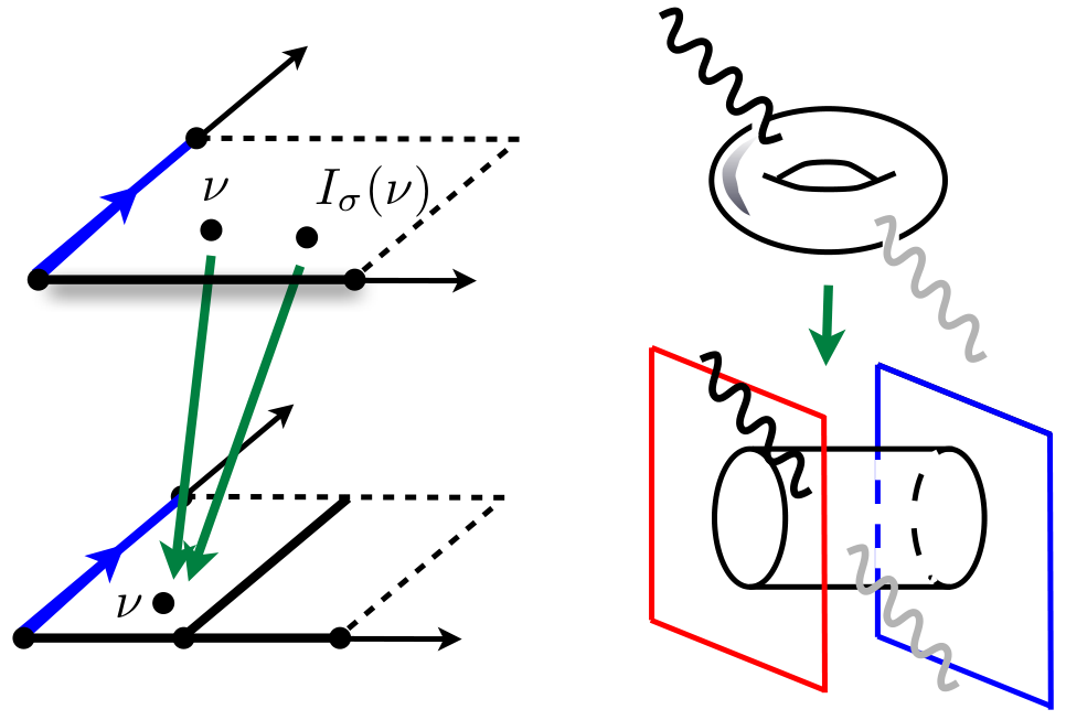
Figure 2: The standard way to make the worldsheet surfaces with crosscaps and boundaries, and their Green’s functions, from that of the worldsheet torus is by identifying under a certain involution.

Using the worldsheet correlators of appendices §C and §D we have for the torus amplitude σ=𝒯\sigma=\mathcal{T}:

⟨VZ​Z¯(p1)VZ​Z¯(p2)⟩𝒯s,s~|Fourfermions=−2δ∫𝒯d2ν1∫𝒯d2ν2e−δ​GB𝒯​(ν1,ν2)\displaystyle\langle V_{Z\bar{Z}}(p_{1})V_{Z\bar{Z}}(p_{2})\rangle_{\mathcal{T}}^{s,\tilde{s}}\big|_{\begin{subarray}{c}\text{Four}~~~~\,\\ \text{fermions}\end{subarray}}=-2\,\delta\int_{\mathcal{T}}\text{d}^{2}\nu_{1}\int_{\mathcal{T}}\text{d}^{2}\nu_{2}\,e^{-\delta G_{B}^{\mathcal{T}}(\nu_{1},\,\nu_{2})}
×{[(∂1∂2GB−γ→)(ν1,ν2)]∗GFγ→(s;ν2,ν1)GF(s;ν2,ν1)\displaystyle~~~~~~~~~~\times\Big\{\big[(\partial_{1}\partial_{2}G_{B}^{-\vec{\gamma}})(\nu_{1},\nu_{2})\big]^{*}\,G_{F}^{\vec{\gamma}}(s;\nu_{2},\nu_{1})\,G_{F}(s;\nu_{2},\nu_{1})
+(∂1∂2GBγ→)(ν1,ν2)[GF−γ→(s~;ν2,ν1)]∗[GF(s~;ν2,ν1)]∗},\displaystyle~~~~~~~~~~~+(\partial_{1}\partial_{2}G_{B}^{\vec{\gamma}})(\nu_{1},\nu_{2})\,\big[G_{F}^{-\vec{\gamma}}(\tilde{s};\nu_{2},\nu_{1})\big]^{*}\,\big[G_{F}(\tilde{s};\nu_{2},\nu_{1})\big]^{*}\Big\}\,, (28)

where we introduced the dimensionless momentum-squared invariant δ\delta as55 5 With strict momentum conservation this would vanish on-shell, but we relax overall momentum conservation as in [29], see p. 19 of [12] for more discussion.

δ≡α′2​(p1⋅p2)\displaystyle\delta\equiv\frac{\alpha^{\prime}}{2}(p_{1}\cdot p_{2}) (29)

and γ→\vec{\gamma} is the twist (quasiperiodicity) of the worldsheet correlator, see appendices §C and §D for details. For the annulus, Möbius strip and Klein bottle amplitudes (σ=𝒜,ℳ,𝒦\sigma={\mathcal{A}},{\mathcal{M}},{\mathcal{K}}) we have:

⟨VZ​Z¯(p1)VZ​Z¯(p2)⟩σs|Fourfermions=−2δ∫σd2ν1∫σd2ν2e−δ​GBσ​(ν1,ν2)\displaystyle\big\langle V_{Z\bar{Z}}(p_{1})V_{Z\bar{Z}}(p_{2})\big\rangle_{\sigma}^{s}\big|_{\begin{subarray}{c}\text{Four}~~~~\,\\ \text{fermions}\end{subarray}}=-2\delta\int_{\sigma}\text{d}^{2}\nu_{1}\int_{\sigma}\text{d}^{2}\nu_{2}\,e^{-\delta G_{B}^{\sigma}(\nu_{1},\,\nu_{2})}
×{(∂¯1∂¯2GBγ)(Iσ(ν1),Iσ(ν2))GFγ(s;ν2,ν1)GF(s;ν2,ν1)\displaystyle~~~~~~~~~~\times\Big\{(\bar{\partial}_{1}\bar{\partial}_{2}G_{B}^{\gamma})(I_{\sigma}(\nu_{1}),I_{\sigma}(\nu_{2}))\,G_{F}^{\gamma}(s;\nu_{2},\nu_{1})\,G_{F}(s;\nu_{2},\nu_{1})\phantom{\Big\}}
−(∂1∂¯2​GBγ)​(ν1,Iσ​(ν2))​GFγ​(s,ν2,Iσ​(ν1))​GF​(s,ν2,Iσ​(ν1))\displaystyle~~~~~~~~~~~~-(\partial_{1}\bar{\partial}_{2}G_{B}^{\gamma})(\nu_{1},I_{\sigma}(\nu_{2}))\,G_{F}^{\gamma}(s;\nu_{2},I_{\sigma}(\nu_{1}))\,G_{F}(s;\nu_{2},I_{\sigma}(\nu_{1}))\phantom{\Big\}}
−(∂¯1​∂2GBγ)​(Iσ​(ν1),ν2)​GFγ​(s,Iσ​(ν2),ν1)​GF​(s,Iσ​(ν2),ν1)\displaystyle~~~~~~~~~~~~-(\bar{\partial}_{1}\partial_{2}G_{B}^{\gamma})(I_{\sigma}(\nu_{1}),\nu_{2})\,G_{F}^{\gamma}(s;I_{\sigma}(\nu_{2}),\nu_{1})\,G_{F}(s;I_{\sigma}(\nu_{2}),\nu_{1})\phantom{\Big\}}
+(∂1∂2GBγ)(ν1,ν2)GFγ(s,Iσ(ν2),Iσ(ν1))GF(s;Iσ(ν2),Iσ(ν1))},\displaystyle~~~~~~~~~~~~+(\partial_{1}\partial_{2}G_{B}^{\gamma})(\nu_{1},\nu_{2})G_{F}^{\gamma}(s,I_{\sigma}(\nu_{2}),I_{\sigma}(\nu_{1}))G_{F}(s;I_{\sigma}(\nu_{2}),I_{\sigma}(\nu_{1}))\Big\}\,, (30)

where there is only a single real twist γ\gamma (related to the orbifold twist, as in table 1 in §3.8) and the definition of the involutions IσI_{\sigma} can be found in the appendix, cf. (182), and see fig. 2. The slightly surprising choice of ordering of arguments in eq. (30) is convenient to absorb some phases that would appear for the more obvious ordering. Note that although most of the correlators refer to the covering torus, at this point the integrals are still performed over each worldsheet surface σ=𝒜,ℳ,𝒦\sigma={\mathcal{A}},{\mathcal{M}},{\mathcal{K}}. We now proceed to lift the world sheet integrals to the covering torus (see fig. 3), using the results of §B.1:

⟨VZ​Z¯​(p1)​VZ​Z¯​(p2)⟩σs|Fourfermions\displaystyle\big\langle V_{Z\bar{Z}}(p_{1})V_{Z\bar{Z}}(p_{2})\big\rangle_{\sigma}^{s}\big|_{\begin{subarray}{c}\text{Four}~~~~\,\\ \text{fermions}\end{subarray}} =−2δ∫𝒯d2ν1∫𝒯d2ν2e−δ​GBσ​(ν1,ν2)\displaystyle=-2\delta\int_{\mathcal{T}}\text{d}^{2}\nu_{1}\int_{\mathcal{T}}\text{d}^{2}\nu_{2}\,e^{-\delta G_{B}^{\sigma}(\nu_{1},\,\nu_{2})}
×(∂¯1​∂¯2​GBγ)​(Iσ​(ν1),Iσ​(ν2))​GFγ​(s,ν2,ν1)​GF​(s,ν2,ν1).\displaystyle\,~~~\times(\bar{\partial}_{1}\bar{\partial}_{2}G_{B}^{\gamma})(I_{\sigma}(\nu_{1}),I_{\sigma}(\nu_{2}))\,G_{F}^{\gamma}(s;\nu_{2},\nu_{1})\,G_{F}(s;\nu_{2},\nu_{1})\,. (31)

As promised, the integration domains with boundaries and crosscaps have been replaced by purely torus integrals,

Refer to caption
Figure 3: A lifting that gives amplitudes for open and unoriented strings from closed strings.

and now most Green’s functions in the integrand also refer to the covering torus. The only remaining Green’s functions on the surface σ\sigma is the GBσG_{B}^{\sigma} in the exponent, and since this has a forefactor that carries momenta, we will be able to treat it separately from the others in the low-energy limit.

In all, what we have done is to provide a simple prescription to compute open and unoriented string (gauge theory-like) loop amplitudes from closed string (gravity-like) loop amplitudes. This is backwards compared to what is done in recent work on field theory amplitude calculations, where one derives gravity amplitudes from gauge theory amplitudes! (See for example one of the original papers [30], and the more recent string theory work in [31].) The lifting procedure is convenient because it allows us to systematize the calculation and make use of known results for torus amplitudes. Note also that the Chan-Paton states are traced over, otherwise this lifting would clearly have been impossible.

Now we go through similar steps for the eight-fermion contributions, which read

⟨VZ​Z¯​(p1)​VZ​Z¯​(p2)⟩σs|Eightfermions\displaystyle\big\langle V_{Z\bar{Z}}(p_{1})V_{Z\bar{Z}}(p_{2})\big\rangle_{\sigma}^{s}\big|_{\begin{subarray}{c}\text{Eight}~~~\,\,\\ \text{fermions}\end{subarray}} =−(α′2)2(p1⋅p2)2∫σd2ν1∫σd2ν2e−(p1⋅p2)​⟨X1​X2⟩σ\displaystyle=-\left(\frac{\alpha^{\prime}}{2}\right)^{2}(p_{1}\cdot p_{2})^{2}\int_{\sigma}\text{d}^{2}\nu_{1}\int_{\sigma}\text{d}^{2}\nu_{2}\,e^{-(p_{1}\cdot\,p_{2})\,\langle X_{1}X_{2}\rangle_{\sigma}}
×{⟨ψ1​ψ2⟩σs​⟨ψ~1​ψ~2⟩σs−⟨ψ1​ψ~2⟩σs​⟨ψ~1​ψ2⟩σs}\displaystyle~~~\,\times\Big\{\langle\psi_{1}\psi_{2}\rangle_{\sigma}^{s}\langle\tilde{\psi}_{1}\tilde{\psi}_{2}\rangle_{\sigma}^{s}-\langle\psi_{1}\tilde{\psi}_{2}\rangle_{\sigma}^{s}\langle\tilde{\psi}_{1}\psi_{2}\rangle_{\sigma}^{s}\Big\}
×{⟨Ψ1Ψ¯2⟩σs⟨Ψ~2Ψ¯~1⟩σs−⟨Ψ~1Ψ¯2⟩σs⟨Ψ~2Ψ¯1⟩σs\displaystyle~~~\,\times\Big\{\langle\Psi_{1}\bar{\Psi}_{2}\rangle_{\sigma}^{s}\langle\tilde{\Psi}_{2}\tilde{\bar{\Psi}}_{1}\rangle_{\sigma}^{s}-\langle\tilde{\Psi}_{1}\bar{\Psi}_{2}\rangle_{\sigma}^{s}\langle\tilde{\Psi}_{2}\bar{\Psi}_{1}\rangle_{\sigma}^{s}
−⟨Ψ1Ψ¯~2⟩σs⟨Ψ2Ψ¯~1⟩σs+⟨Ψ~1Ψ¯~2⟩σs⟨Ψ2Ψ¯1⟩σs}.\displaystyle~~~~~\,-\langle\Psi_{1}\tilde{\bar{\Psi}}_{2}\rangle_{\sigma}^{s}\langle\Psi_{2}\tilde{\bar{\Psi}}_{1}\rangle_{\sigma}^{s}+\langle\tilde{\Psi}_{1}\tilde{\bar{\Psi}}_{2}\rangle_{\sigma}^{s}\langle\Psi_{2}\bar{\Psi}_{1}\rangle_{\sigma}^{s}\Big\}\;. (32)

Again with the worldsheet correlators of appendices §C and §D we have for σ=𝒯\sigma=\mathcal{T}

⟨VZ​Z¯​(p1)​VZ​Z¯​(p2)⟩𝒯s,s~|Eightfermions\displaystyle\big\langle V_{Z\bar{Z}}(p_{1})V_{Z\bar{Z}}(p_{2})\big\rangle_{\mathcal{T}}^{s,\tilde{s}}\big|_{\begin{subarray}{c}\text{Eight}~~~\,\,\\ \text{fermions}\end{subarray}} =−2δ2∫𝒯d2ν1∫𝒯d2ν2e−δ​GB𝒯​(ν1,ν2)\displaystyle=-2\delta^{2}\int_{\mathcal{T}}\text{d}^{2}\nu_{1}\int_{\mathcal{T}}\text{d}^{2}\nu_{2}\,e^{-\delta G_{B}^{\mathcal{T}}(\nu_{1},\nu_{2})}
×GF​(s,ν1,ν2)​[GF​(s~,ν1,ν2)]∗​GFγ→​(s,ν1,ν2)​[GF−γ→​(s~,ν2,ν1)]∗,\displaystyle\times G_{F}(s;\nu_{1},\nu_{2})\,[G_{F}(\tilde{s};\nu_{1},\nu_{2})]^{*}\,G_{F}^{\vec{\gamma}}(s;\nu_{1},\nu_{2})\,[G_{F}^{-\vec{\gamma}}(\tilde{s};\nu_{2},\nu_{1})]^{*}\,, (33)

and for σ=𝒜,ℳ,𝒦\sigma={\mathcal{A}},{\mathcal{M}},{\mathcal{K}}

⟨VZ​Z¯(p1)VZ​Z¯(p2)⟩σs|Eightfermions=−δ2∫σd2ν1∫σd2ν2e−δ​GBσ​(ν1,ν2)\displaystyle\big\langle V_{Z\bar{Z}}(p_{1})V_{Z\bar{Z}}(p_{2})\big\rangle_{\sigma}^{s}\big|_{\begin{subarray}{c}\text{Eight}~~~\,\,\\ \text{fermions}\end{subarray}}=-\delta^{2}\int_{\sigma}\text{d}^{2}\nu_{1}\int_{\sigma}\text{d}^{2}\nu_{2}\,e^{-\delta G_{B}^{\sigma}(\nu_{1},\,\nu_{2})}
×{GF​(s,ν1,ν2)​GF​(s,Iσ​(ν1),Iσ​(ν2))−GF​(s,ν1,Iσ​(ν2))​GF​(s,Iσ​(ν1),ν2)}\displaystyle~~~~~~~~~~~\times\Big\{\,G_{F}(s;\nu_{1},\nu_{2})\,G_{F}(s;I_{\sigma}(\nu_{1}),I_{\sigma}(\nu_{2}))-G_{F}(s;\nu_{1},I_{\sigma}(\nu_{2}))\,G_{F}(s;I_{\sigma}(\nu_{1}),\nu_{2})\Big\}
×{GFγ(s;ν1,ν2)GFγ(s;Iσ(ν2),Iσ(ν1))\displaystyle~~~~~~~~~~~\times\Big\{\,G_{F}^{\gamma}(s;\nu_{1},\nu_{2})\,G_{F}^{\gamma}(s;I_{\sigma}(\nu_{2}),I_{\sigma}(\nu_{1}))\phantom{\Big\}}
−GFγ​(s,Iσ​(ν1),ν2)​GFγ​(s,Iσ​(ν2),ν1)​e2​π​i​γ​δσ​𝒦\displaystyle~~~~~~~~~~~~~\,-G_{F}^{\gamma}(s;I_{\sigma}(\nu_{1}),\nu_{2})\,G_{F}^{\gamma}(s;I_{\sigma}(\nu_{2}),\nu_{1})\,e^{2\pi i\gamma\delta_{\sigma\mathcal{K}}}\phantom{\Big\}}
−GFγ​(s,ν1,Iσ​(ν2))​GFγ​(s,ν2,Iσ​(ν1))​e−2​π​i​γ​δσ​𝒦\displaystyle~~~~~~~~~~~~~\,-G_{F}^{\gamma}(s;\nu_{1},I_{\sigma}(\nu_{2}))\,G_{F}^{\gamma}(s;\nu_{2},I_{\sigma}(\nu_{1}))\,e^{-2\pi i\gamma\delta_{\sigma\mathcal{K}}}\phantom{\Big\}}
+GFγ(s;Iσ(ν1),Iσ(ν2))GF(s;ν2,ν1)}.\displaystyle~~~~~~~~~~~~~\,+G_{F}^{\gamma}(s;I_{\sigma}(\nu_{1}),I_{\sigma}(\nu_{2}))\,G_{F}(s;\nu_{2},\nu_{1})\Big\}\,. (34)

Now we can use the results of §B.1 again to lift the world sheet integrals to the covering torus:

⟨VZ​Z¯(p1)VZ​Z¯(p2)⟩σs|Eightfermions=−δ2∫𝒯d2ν1∫𝒯d2ν2e−δ​GBσ​(ν1,ν2)\displaystyle\big\langle V_{Z\bar{Z}}(p_{1})V_{Z\bar{Z}}(p_{2})\big\rangle_{\sigma}^{s}\big|_{\begin{subarray}{c}\text{Eight}~~~\,\,\\ \text{fermions}\end{subarray}}=-\delta^{2}\int_{\mathcal{T}}\text{d}^{2}\nu_{1}\int_{\mathcal{T}}\text{d}^{2}\nu_{2}\,e^{-\delta G_{B}^{\sigma}(\nu_{1},\,\nu_{2})}
×{GF​(s,ν1,ν2)​GF​(s,Iσ​(ν1),Iσ​(ν2))−GF​(s,ν1,Iσ​(ν2))​GF​(s,Iσ​(ν1),ν2)}\displaystyle~~~~~~~~~~~\times\Big\{\,G_{F}(s;\nu_{1},\nu_{2})\,G_{F}(s;I_{\sigma}(\nu_{1}),I_{\sigma}(\nu_{2}))\,-G_{F}(s;\nu_{1},I_{\sigma}(\nu_{2}))\,G_{F}(s;I_{\sigma}(\nu_{1}),\nu_{2})\Big\}
×GFγ​(s,ν1,ν2)​GFγ​(s,Iσ​(ν2),Iσ​(ν1)).\displaystyle~~~~~~~~~~~\times\,G_{F}^{\gamma}(s;\nu_{1},\nu_{2})\,G_{F}^{\gamma}(s;I_{\sigma}(\nu_{2}),I_{\sigma}(\nu_{1}))\;. (35)

3.1 Four fermions

Let us start with the four-fermion terms. We first note that the torus amplitude (28) does not contribute. This is due to the fact that the two contributions from the Green’s functions only depend either exclusively on the left moving spin structure or the right moving spin structure. Then, multiplying (28) with the partition functions and summing over both the left and the right moving spin structures produces zero.

Thus, we are left with the four-fermion terms in eq. (31). We consider the untwisted Kähler modulus of the third torus. Then all the relevant correlators have Neumann-Neumann boundary conditions, no matter what surface we consider. Let us concentrate on the spin structure dependent terms, i.e. the partition function and the two fermion Green’s functions. It is useful to define ZsϑZ_{s}^{\vartheta}, the part of the partition function that contains the Jacobi theta functions, which we give explicitly in eq. (278). With this notation, we perform the spin structure sum and obtain just a single Green’s function:

∑sηs​Zsϑ​GFγ​(s,ν2,ν1)​GF​(s,ν2,ν1)=GFγ​(ν2,ν1).\displaystyle\sum_{s}\eta_{s}Z_{s}^{\vartheta}G_{F}^{\gamma}(s;\nu_{2},\nu_{1})\,G_{F}(s;\nu_{2},\nu_{1})=G_{F}^{\gamma}(\nu_{2},\nu_{1})\,. (36)

Here we use the following convention: if we do not indicate explicitly over which spin structure ss to sum, it is over even spin structures (s=2,3,4s=2,3,4). We show (36) in §G.1. The GSO sign ηs\eta_{s} is given in table 2 in appendix §D. What happened is that (non-manifest) supersymmetry reduced the number of Green’s functions in the integrand. We introduced a new convention on the right hand side: if we do not indicate the spin structure ss explicitly for a fermion Green’s function, it is s=1s=1 (odd). Now we can calculate

∑sηs​Zsϑ​⟨VZ​Z¯​(p1)​VZ​Z¯​(p2)⟩σs|Fourfermions\displaystyle\sum_{s}\eta_{s}Z_{s}^{\vartheta}\big\langle V_{Z\bar{Z}}(p_{1})V_{Z\bar{Z}}(p_{2})\big\rangle_{\sigma}^{s}\big|_{\begin{subarray}{c}\text{Four}~~~~\,\\ \text{fermions}\end{subarray}}
=−2δ∫𝒯d2ν1∫𝒯d2ν2e−δ​GBσ​(ν1,ν2)GFγ(ν2,ν1)∂¯2GFγ(Iσ(ν1),Iσ(ν2)),\displaystyle=-2\delta\int_{\mathcal{T}}\text{d}^{2}\nu_{1}\int_{\mathcal{T}}\text{d}^{2}\nu_{2}\,e^{-\delta G_{B}^{\sigma}(\nu_{1},\,\nu_{2})}\,G_{F}^{\gamma}(\nu_{2},\nu_{1})\bar{\partial}_{2}G_{F}^{\gamma}(I_{\sigma}(\nu_{1}),I_{\sigma}(\nu_{2}))\,, (37)

where we used the identity ∂¯1​∂¯2​GBγ​(Iσ​(ν1),Iσ​(ν2))=∂¯2​GFγ​(Iσ​(ν1),Iσ​(ν2))\bar{\partial}_{1}\bar{\partial}_{2}G_{B}^{\gamma}(I_{\sigma}(\nu_{1}),I_{\sigma}(\nu_{2}))=\bar{\partial}_{2}G_{F}^{\gamma}(I_{\sigma}(\nu_{1}),I_{\sigma}(\nu_{2})) to replace a boson Green’s function with a fermion Green’s function. (Note that before differentiation, the boson propagator depends on both ν\nu and ν¯=Iσ​(ν1)−Iσ​(ν2)\bar{\nu}=I_{\sigma}(\nu_{1})-I_{\sigma}(\nu_{2}). We only display the dependence on one of them in the argument, and choose freely which one to display. The fermion propagator of course only depends on either ν\nu or ν¯\bar{\nu}. )

3.2 Evaluation by analytic continuation

In the limit δ→0\delta\to 0 the integrand in eq. (37) is a function of the relative coordinates ν≡ν2−ν1\nu\equiv\nu_{2}-\nu_{1} and ν¯≡Iσ​(ν1)−Iσ​(ν2)\bar{\nu}\equiv I_{\sigma}(\nu_{1})-I_{\sigma}(\nu_{2}) only. We change variables and trivially integrate over the “center-of-mass” coordinate. Setting GFγ​(ν,0)≡GFγ​(ν)G_{F}^{\gamma}(\nu,0)\equiv G_{F}^{\gamma}(\nu) we obtain

∑sηsZsϑ⟨VZ​Z¯(p1)VZ​Z¯(p2)⟩σs|Fourfermions=−4τ2δ∫𝒯d2νGFγ(ν)∂¯GFγ(ν¯)+𝒪(δ2),\displaystyle\sum_{s}\eta_{s}Z_{s}^{\vartheta}\big\langle V_{Z\bar{Z}}(p_{1})V_{Z\bar{Z}}(p_{2})\big\rangle_{\sigma}^{s}\big|_{\begin{subarray}{c}\text{Four}~~~~\,\\ \text{fermions}\end{subarray}}=-4\tau_{2}\delta\int_{\mathcal{T}}\text{d}^{2}\nu\,G_{F}^{\gamma}(\nu)\bar{\partial}G_{F}^{\gamma}(\bar{\nu})+\mathscr{O}(\delta^{2})\,, (38)

where the 2​τ22\tau_{2} is from the trivial integral.

Naively, the integral in eq. (38) appears divergent since the integrand is singular at the lattice points ν=ℤ+τ​ℤ\nu=\mathbb{Z}+\tau\mathbb{Z}. However, when adding the contributions from the four corner points 0,1,τ0,1,\tau and 1+τ1+\tau we find that the divergences cancel. To see this, since the integrand in eq. (38) is doubly periodic we can shift the integration region such that the only enclosed lattice point is the origin ν=0\nu=0, as in fig. 4.

Figure 4: The integrand is not invariant under a half-integer shift, but the integral over the fundamental domain is. In this figure, each quarter-piece of integration domain is mapped by an integer lattice shift.

Close to ν=0\nu=0 the integrand behaves as

GFγ​(ν)​∂¯​GFγ​(ν¯)=−1ν​ν¯2−c0​1ν¯2−c1​νν¯2+c1​1ν+finite,\displaystyle G_{F}^{\gamma}(\nu)\bar{\partial}G_{F}^{\gamma}(\bar{\nu})=-\frac{1}{\nu\bar{\nu}^{2}}-c_{0}\,\frac{1}{\bar{\nu}^{2}}-c_{1}\frac{\nu}{\bar{\nu}^{2}}+c_{1}\frac{1}{\nu}+\text{finite}\,, (39)

where c0c_{0} and c1c_{1} are the first two coefficients from the expansion GFγ​(ν)=1ν+c0+c1​ν+𝒪⁡(ν2)G_{F}^{\gamma}(\nu)=\frac{1}{\nu}+c_{0}+c_{1}\nu+\mathscr{O}(\nu^{2}). Because the same number of powers of ν\nu and ν¯\bar{\nu} never occur together, the integral of eq. (39) over an infinitesimal disk centered at ν=0\nu=0 must vanish:

limε→0∫|ν|≤εd2​ν​GFγ​(ν)​∂¯​GFγ​(ν¯)\displaystyle\lim_{\varepsilon\to 0}\int_{|\nu|\leq\varepsilon}\text{d}^{2}\nu\,G_{F}^{\gamma}(\nu)\bar{\partial}G_{F}^{\gamma}(\bar{\nu})
=2​limε→0∫0εd​r​r​∫02​πd​θ​[−ei​θr3−c0​e2​i​θr2−c1​e3​i​θr+c1​e−i​θr+finite]=0,\displaystyle=2\lim_{\varepsilon\to 0}\int_{0}^{\varepsilon}\text{d}r\,r\int_{0}^{2\pi}\text{d}\theta\left[-\frac{e^{i\theta}}{r^{3}}-c_{0}\frac{e^{2i\theta}}{r^{2}}-c_{1}\frac{e^{3i\theta}}{r}+c_{1}\frac{e^{-i\theta}}{r}+\text{finite}\right]=0\,, (40)

where the factor of 22 in the second row arises from d2​ν=2​d​(Re⁡ν)​d​(Im⁡ν)\text{d}^{2}\nu=2\,\text{d}(\Re\nu)\,\text{d}(\Im\nu). We changed to polar coordinates via ν=r​ei​θ\nu=re^{i\theta} and used ∫02​πd​θ​ei​m​θ=0\int_{0}^{2\pi}\text{d}\theta\,e^{im\theta}=0 for all m∈ℤ\{0}m\in\mathbb{Z}\backslash\{0\}.

We have argued that the integral in eq. (38) is finite, but finiteness is not manifest. To calculate the finite value explicitly we will use analytic continuation: we introduce a complex parameter ss (not to be confused with the spin structure, which is also denoted ss) and define a meromorphic function F⁡(s)F(s) whose value at s=1s=1 is the desired integral. This may seem roundabout for calculating a finite value, but we will find that evaluation in some other region of the complex ss plane is quite simple, and we believe that some of the intermediate steps could be of general interest. For completeness, we rederive the result by two alternative approaches in the appendix: partial integration and point splitting, in §H and §I, respectively.

In §E.1 we identify the Green’s functions of bosons and fermions on the torus in terms of Eisenstein-Kronecker functions E1E_{1}:

GBγ​(ν)\displaystyle G_{B}^{\gamma}(\nu) =E1​(γ,ν)+const.,\displaystyle=E_{1}(\gamma,\nu)+\mathrm{const.}\,,\quad (41)
GFγ​(ν)\displaystyle G_{F}^{\gamma}(\nu) =−∂νE1(γ,ν).\displaystyle=-\partial_{\nu}E_{1}(\gamma,\nu)\,. (42)

The Eisenstein-Kronecker functions (see e.g. Ch. 8 of [32]) are defined for any complex numbers ww and zz and for Re⁡s>1\Re s>1 by

Es​(w,z)=(τ2π)s​∑m,n′exp⁡(2​π​iτ2​Im⁡[(w+m+n​τ)​z¯])|w+m+n​τ|2​s,\displaystyle E_{s}(w,z)=\left(\frac{\tau_{2}}{\pi}\right)^{s}{\sum_{m,n}}^{\prime}\,\,\frac{\exp(\frac{2\pi i}{\tau_{2}}\Im[(w+m+n\tau)\bar{z}])}{|w+m+n\tau|^{2s}}\,, (43)

where by ∑m,n′\sum_{m,n}^{\prime} we intend the sum over all m,n∈ℤm,n\in\mathbb{Z} such that w+m+n​τ≠0w+m+n\tau\neq 0. For Re⁡s>12\Re s>{\frac{1}{2}} the series converges almost everywhere, i.e. away from z∈ℤ+τ​ℤz\in\mathbb{Z}+\tau\mathbb{Z}, and in particular for s=1s=1 the series converges to the boson Green’s function. For other values of ss the Eisenstein-Kronecker function is defined by analytic continuation.

Now, we define a new function F=F⁡(s)F=F(s) of the complex parameter ss, whose value at s=1s=1 gives the desired worldsheet integral

F⁡(s):=∫𝒯d2​ν​∂Es​(γ,ν)​∂¯2​Es​(γ,ν¯),F⁡(1)=∫𝒯d2​ν​GFγ​(ν)​∂¯​GFγ​(ν¯).\displaystyle F(s):=\int_{\mathcal{T}}\text{d}^{2}\nu\,\partial E_{s}(\gamma,\nu)\bar{\partial}^{2}E_{s}(\gamma,\bar{\nu})\,,\quad F(1)=\int_{\mathcal{T}}\text{d}^{2}\nu\,G_{F}^{\gamma}(\nu)\bar{\partial}G_{F}^{\gamma}(\bar{\nu})\,. (44)

The motivation for studying F⁡(s)F(s) rather than F⁡(1)F(1) directly is that by taking Re⁡s\Re s large enough, the integrand becomes manifestly finite everywhere in the integration region. Now, we have

F⁡(s)=(−1)3​∫d2​ν\displaystyle F(s)=(-1)^{3}\,\int\text{d}^{2}\nu\, (τ2π)s−1​∑k,ℓγ+k+ℓ​τ¯|γ+k+ℓ​τ|2​s​e2​π​iτ2​Im⁡[(γ+k+ℓ​τ)​ν¯]\displaystyle\left(\frac{\tau_{2}}{\pi}\right)^{s-1}\sum_{k,\ell}\frac{\gamma+k+\ell\bar{\tau}}{|\gamma+k+\ell\tau|^{2s}}\,e^{\frac{2\pi i}{\tau_{2}}\Im[(\gamma+k+\ell\tau)\bar{\nu}]}
×\displaystyle\times (τ2π)s−2​∑m,n(γ+m+n​τ¯)2|γ+m+n​τ|2​s​e2​π​iτ2​Im⁡[(γ+m+n​τ)​ν].\displaystyle\left(\frac{\tau_{2}}{\pi}\right)^{s-2}\sum_{m,n}\,\frac{(\gamma+m+n\bar{\tau})^{2}}{|\gamma+m+n\tau|^{2s}}\,e^{\frac{2\pi i}{\tau_{2}}\Im[(\gamma+m+n\tau)\nu]}\,. (45)

Using the orthogonality relation

∫d2​ν​e2​π​iτ2​Im⁡[(γ+k+ℓ​τ)​ν¯]​e2​π​iτ2​Im⁡[(γ+m+n​τ)​ν]=2​τ2​δℓ,−n​δk,m+n​δσ​ℳ,\displaystyle\int\text{d}^{2}\nu\,e^{\frac{2\pi i}{\tau_{2}}\Im[(\gamma+k+\ell\tau)\bar{\nu}]}\,e^{\frac{2\pi i}{\tau_{2}}\Im[(\gamma+m+n\tau)\nu]}=2\tau_{2}\,\delta_{\ell,-n}\,\delta_{k,m+n\delta_{\sigma{\mathcal{M}}}}\,, (46)

which follows from τ¯=−τ+δσ​ℳ\bar{\tau}=-\tau+\delta_{\sigma{\mathcal{M}}}, we arrive at

F⁡(s)\displaystyle F(s) =−2π(τ2π)2​s−2∑m,n(γ+m+n​δσ​ℳ−n​τ¯)​(γ+m+n​τ¯)2|γ+m+n​δσ​ℳ−n​τ|2​s​|γ+m+n​τ|2​s,\displaystyle=-2\pi\left(\frac{\tau_{2}}{\pi}\right)^{2s-2}\sum_{m,n}\frac{(\gamma+m+n\delta_{\sigma{\mathcal{M}}}-n\bar{\tau})(\gamma+m+n\bar{\tau})^{2}}{|\gamma+m+n\delta_{\sigma{\mathcal{M}}}-n\tau|^{2s}|\gamma+m+n\tau|^{2s}}\,, (47)
=−2π(τ2π)2​s−2∑m,nγ+m+n​τ¯|γ+m+n​τ|2​(2​s−1).\displaystyle=-2\pi\left(\frac{\tau_{2}}{\pi}\right)^{2s-2}\sum_{m,n}\frac{\gamma+m+n\bar{\tau}}{|\gamma+m+n\tau|^{2(2s-1)}}\,. (48)

We now temporarily (eq. (49) through eq. (51)) treat γ\gamma and γ¯\bar{\gamma} as independent variables and only in the end we specify to real γ\gamma. Then we can write eq. (48) as

F⁡(s)\displaystyle F(s) =2​π​∂∂γ​[12​s−2​(τ2π)2​s−2​∑m,n1|γ+m+n​τ|2​(2​s−2)]|γ​real=2​π​∂∂γ​[E2​s−2​(γ,0)2​s−2]|γ​real.\displaystyle=2\pi\frac{\partial}{\partial\gamma}\bigg[\frac{1}{2s-2}\left(\frac{\tau_{2}}{\pi}\right)^{2s-2}\sum_{m,n}\frac{1}{|\gamma+m+n\tau|^{2(2s-2)}}\bigg]\bigg|_{\gamma\,\mathrm{real}}=2\pi\frac{\partial}{\partial\gamma}\bigg[\frac{E_{2s-2}(\gamma,0)}{2s-2}\bigg]\bigg|_{\gamma\,\mathrm{real}}\,. (49)

The right-hand side defines the analytic continuation of F⁡(s)F(s) to the whole complex plane.

In the limit s→1s\to 1 we have

E2​s−2​(γ,0)2​s−2=E0​(γ,0)2​s−2+E0′​(γ,0)+…\displaystyle\frac{E_{2s-2}(\gamma,0)}{2s-2}=\frac{E_{0}(\gamma,0)}{2s-2}+E_{0}^{\prime}(\gamma,0)+\ldots (50)

and E0​(γ,0)=0E_{0}(\gamma,0)=0, E0′​(γ,0)=E1​(0,γ)E_{0}^{\prime}(\gamma,0)=E_{1}(0,\gamma), which is given by Kronecker’s second limit formula

E1​(0,γ)=−ln⁡|ϑ1​(γ,τ)η⁡(τ)|2+2​πτ2​(Im⁡γ)2,\displaystyle E_{1}(0,\gamma)=-\ln\left|\frac{\vartheta_{1}(\gamma,\tau)}{\eta(\tau)}\right|^{2}+\frac{2\pi}{\tau_{2}}(\Im\gamma)^{2}\,, (51)

as we show in §E.1 for completeness. When evaluating ∂γE1|γ​real\partial_{\gamma}E_{1}|_{\gamma\,\mathrm{real}} the second term vanishes and we conclude for F⁡(s)F(s) at s=1s=1:

F⁡(1)=−2​π​ϑ1′​(γ,τσ)ϑ1​(γ,τσ).\displaystyle F(1)=-2\pi\frac{\vartheta_{1}^{\prime}(\gamma,\tau_{\sigma})}{\vartheta_{1}(\gamma,\tau_{\sigma})}\,. (52)

Thus we find the four-fermion term

∑sηs​Zsϑ​⟨VZ​Z¯​(p1)​VZ​Z¯​(p2)⟩σ=8​π​τ2​δ​ϑ1′​(γ,τ)ϑ1​(γ,τ),\displaystyle\sum_{s}\eta_{s}Z_{s}^{\vartheta}\langle V_{Z\bar{Z}}(p_{1})V_{Z\bar{Z}}(p_{2})\rangle_{\sigma}=8\pi\tau_{2}\delta\,\frac{\vartheta_{1}^{\prime}(\gamma,\tau)}{\vartheta_{1}(\gamma,\tau)}\,, (53)

which agrees with the alternative calculations in §H and §I.

3.3 Eight-fermion term: General arguments

Let us now move on to the eight-fermion term 35. We first focus on σ=𝒜,ℳ,𝒦\sigma={\mathcal{A}},{\mathcal{M}},{\mathcal{K}} and come back to the torus contribution in §3.7. For 𝒩=4{\mathcal{N}}=4 sectors, the eight-fermion term gave the full result for higher-curvature corrections [33]. Since the eight-fermion term has four explicit momentum factors in front, it can only contribute at order α′​p2\alpha^{\prime}p^{2} if there is a pole 1/δ=2/(α′​p1⋅p2)1/\delta=2/(\alpha^{\prime}p_{1}\cdot p_{2}) from vertex collisions. For 𝒩=2{\mathcal{N}}=2 sectors, there is no pole, so this term does not contribute at all to renormalization at order α′​p2\alpha^{\prime}p^{2} . We will see this below, and we will also see that for 𝒩=1{\mathcal{N}}=1 sectors there is a pole. A more efficient way to compute it might be to first change the superghost picture, which can reduce the number of explicit factors of momentum so that one does not have to extract a pole, but we will not attempt that possibly instructive calculation in this paper.

Although the present calculation will be longer than the one for the four-fermion term in the previous section, we will find that it reduces to an expression that is very similar to eq. (53). Probably there is a more direct way to see this, perhaps by worldsheet supersymmetry.

We now return to the lifted eight-fermion term of eq. (35):

S≡−δ2∫𝒯d2ν1∫𝒯d2ν2e−δ​GBσ​(ν1,ν2)f(ν1,ν2),\displaystyle S\equiv-\delta^{2}\int_{\mathcal{T}}\text{d}^{2}\nu_{1}\int_{\mathcal{T}}\text{d}^{2}\nu_{2}\,e^{-\delta\,G_{B}^{\sigma}(\nu_{1},\,\nu_{2})}\,\,f(\nu_{1},\nu_{2}), (54)

where ff is

f⁡(ν1,ν2)={GF​(s,ν1,ν2)​GF​(s,Iσ​(ν1),Iσ​(ν2))−GF​(s,ν1,Iσ​(ν2))​GF​(s,Iσ​(ν1),ν2)}\displaystyle f(\nu_{1},\nu_{2})=\Big\{\,G_{F}\big(s;\nu_{1},\nu_{2}\big)\,G_{F}\big(s;I_{\sigma}(\nu_{1}),I_{\sigma}(\nu_{2})\big)\,-G_{F}\big(s;\nu_{1},I_{\sigma}(\nu_{2})\big)\,G_{F}\big(s;I_{\sigma}(\nu_{1}),\nu_{2}\big)\Big\}
×GFγ​(s,ν1,ν2)​GFγ​(s,Iσ​(ν2),Iσ​(ν1)).\displaystyle~~~~~~~~~~~\times\,G_{F}^{\gamma}\big(s;\nu_{1},\nu_{2}\big)\,G_{F}^{\gamma}\big(s;I_{\sigma}(\nu_{2}),I_{\sigma}(\nu_{1})\big)\;. (55)

One can check that ff as a whole is doubly periodic on the covering torus, i.e.

f⁡(ν1,ν2)=f⁡(ν1+1,ν2)=f⁡(ν1,ν2+1)=f⁡(ν1+τ,ν2)=f⁡(ν1,ν2+τ)\displaystyle f(\nu_{1},\nu_{2})=f(\nu_{1}+1,\nu_{2})=f(\nu_{1},\nu_{2}+1)=f(\nu_{1}+\tau,\nu_{2})=f(\nu_{1},\nu_{2}+\tau) (56)

using:

Iσ​(ν+1)=Iσ​(ν)−1,Iσ​(ν+τ)=Iσ​(ν)−τ¯=Iσ​(ν)+τ−δσ​ℳ.\displaystyle I_{\sigma}(\nu+1)=I_{\sigma}(\nu)-1,\,\,I_{\sigma}(\nu+\tau)=I_{\sigma}(\nu)-{\bar{\tau}}=I_{\sigma}(\nu)+\tau-\delta_{\sigma\,\mathcal{M}}\;. (57)

The cancellation of phases that ensures double periodicity as in 56 is fairly nontrivial for the Möbius strip, but it works. We are interested in terms in SS of order δ\delta. In other words, since SS has an overall factor δ2\delta^{2}, we want to compute

F=Sδ|δ→0={−δ∫𝒯d2ν2∫𝒯d2ν1e−δ​GBσ​(ν1,ν2)f(ν1,ν2)}δ→0.\displaystyle F=\left.\frac{S}{\delta}\right|_{\delta\rightarrow 0}=\left\{-\delta\int_{\mathcal{T}}\text{d}^{2}\nu_{2}\int_{\mathcal{T}}\text{d}^{2}\nu_{1}\,e^{-\delta\,G_{B}^{\sigma}(\nu_{1},\,\nu_{2})}\,\,f(\nu_{1},\nu_{2})\right\}_{\delta\rightarrow 0}. (58)

In the limit δ→0\delta\rightarrow 0 the only contribution to the integral on the right hand side arises from vertex operator collisions, i.e. from the integration regions with ν1→ν2\nu_{1}\rightarrow\nu_{2} or ν1→Iσ​(ν2)\nu_{1}\rightarrow I_{\sigma}(\nu_{2}). This can lead to an additional factor 1/δ1/\delta, which then cancels the explicit factor of δ\delta and leads to a finite result. In principle, a similar factor of 1/δ1/\delta could also arise from integrating FF over the world-sheet modulus tt, but we will argue in a moment that this does not occur. Thus, the range of integration in (58) can effectively be restricted to the fundamental domain for one of the vertex operator positions (let us choose ν2\nu_{2}) and disks of infinitesimal radius for ν1\nu_{1} around ν2\nu_{2} and Iσ​(ν2)I_{\sigma}(\nu_{2}). Therefore, schematically we need to calculate (and sum) integrals of the form

F=limε→0{−δ∫𝒯d2ν2∫Dεd2ν1e−δ​GBσ​(ν1,ν2)f(ν1,ν2)}δ→0,\displaystyle F=\lim_{\varepsilon\to 0}\left\{-\delta\int_{\mathcal{T}}\text{d}^{2}\nu_{2}\int_{D_{\varepsilon}}\text{d}^{2}\nu_{1}\,e^{-\delta\,G_{B}^{\sigma}(\nu_{1},\,\nu_{2})}\,\,f(\nu_{1},\nu_{2})\right\}_{\delta\rightarrow 0}, (59)

where DεD_{\varepsilon} is a disk of radius ε\varepsilon around ν2\nu_{2} or Iσ​(ν2)I_{\sigma}(\nu_{2}) (whose dependence on ν2\nu_{2} we keep implicit). We can now expand ff around poles and isolate the terms which survive the δ→0\delta\to 0 limit. At this point it is useful to separate ff as

f=f1−f2,\displaystyle f=f_{1}-f_{2}, (60)

where

f1\displaystyle f_{1} =\displaystyle= GF​(s,ν1,ν2)​GF​(s,Iσ​(ν1),Iσ​(ν2))​GFγ​(s,ν1,ν2)​GFγ​(s,Iσ​(ν2),Iσ​(ν1)),\displaystyle G_{F}\big(s;\nu_{1},\nu_{2}\big)\,G_{F}\big(s;I_{\sigma}(\nu_{1}),I_{\sigma}(\nu_{2})\big)\,G_{F}^{\gamma}\big(s;\nu_{1},\nu_{2}\big)\,G_{F}^{\gamma}\big(s;I_{\sigma}(\nu_{2}),I_{\sigma}(\nu_{1})\big)\ , (61)
f2\displaystyle f_{2} =\displaystyle= GF​(s,ν1,Iσ​(ν2))​GF​(s,Iσ​(ν1),ν2)​GFγ​(s,ν1,ν2)​GFγ​(s,Iσ​(ν2),Iσ​(ν1)).\displaystyle G_{F}\big(s;\nu_{1},I_{\sigma}(\nu_{2})\big)\,G_{F}\big(s;I_{\sigma}(\nu_{1}),\nu_{2}\big)\,G_{F}^{\gamma}\big(s;\nu_{1},\nu_{2}\big)\,G_{F}^{\gamma}\big(s;I_{\sigma}(\nu_{2}),I_{\sigma}(\nu_{1})\big)\;. (62)

Here f1f_{1} has a pole at ν1=ν2\nu_{1}=\nu_{2}, while in addition to this pole f2f_{2} has one more pole at ν1=Iσ​(ν2)\nu_{1}=I_{\sigma}(\nu_{2}) unless ν2=Iσ​(ν2)\nu_{2}=I_{\sigma}(\nu_{2}) modulo torus periodicity. This region is a fixed line under involution and it is the boundary of annulus and Möbius strip worldsheets.

Before we continue with the calculation, a comment about factorization. As stated above, the eight-fermion terms are of order δ2\delta^{2} to start with (recall δ∼α′​p2\delta\sim\alpha^{\prime}p^{2}). In order to contribute to the spacetime kinetic term we are interested in, the integral of (54) over the worldsheet modulus tt would have to provide a factor of δ−1\delta^{-1}. As just mentioned this could in principle either arise from a vertex collision, i.e. from a pole in the integral over ν≡ν1−ν2\nu\equiv\nu_{1}-\nu_{2} (or ν≡ν1−Iσ​(ν2)\nu\equiv\nu_{1}-I_{\sigma}(\nu_{2})), or from the UV region of the tt integral (i.e. from t→0t\rightarrow 0), as in eq. (A.6) of [34]. We will see in the following that there are indeed contributions from vertex collisions. However, we do not expect any additional contributions from the tt integral. The reason can be understood from fig. 5.

Figure 5: One possible factorization of the one-loop two-point function on the annulus.

For ν≠0\nu\neq 0 and t→0t\rightarrow 0 (or equivalently ℓ→∞\ell\rightarrow\infty), the amplitude factorizes as in the lower part of that figure. There are also similar factorization limits of the Möbius and Klein bottle amplitudes that add to the annulus of fig. 5. For the amplitude not to vanish in this factorization limit, there would need to exist a disk coupling (or projective plane coupling, for the unoriented worldsheets) between the modulus TT and some massless closed string state CC (which could be TT itself). In order for this coupling to lead to the δ2\delta^{2} factor in the numerator of the amplitude, the coupling should arise at second order in derivatives, with the δ−1\delta^{-1} factor resulting from the exchange of CC. Thus, for the amplitude not to vanish in this factorization limit, there should be a coupling proportional to ∂μT​∂μC\partial_{\mu}T\partial^{\mu}C at the level of the disk or projective plane. However, it is known that there is no contribution to the kinetic term of the closed string moduli at disk level [24], and similarly we do not expect any contribution from the projective plane. Thus, in the following we will single out vertex collision as the only possible source for a δ−1\delta^{-1} pole in the eight-fermion terms for this amplitude.66 6 A similar argument applied to the four-fermion terms shows the absence of a mass term for the modulus TT.

The expert reader may have realized that in the well-known calculation of mass terms for anomalous U⁡(1)U(1) gauge fields [34], the analogous argument must fail. There the factorization limit of (the analog of the lower panel of) fig. 5 does lead to a non-vanishing contribution at order δ0\delta^{0} to the 2-point function of the gauge fields, signaling a mass term for the naively anomalous U⁡(1)U(1) gauge fields. In their case, the amplitude is of order δ\delta to start with, but a δ−1\delta^{-1} pole arises from the UV-region of the tt integral due to mixing between the anomalous U⁡(1)U(1) gauge field AμA^{\mu} and the RR axion aa at disk level, i.e. a coupling Aμ​∂μaA^{\mu}\partial_{\mu}a. This involves only one derivative, in accordance with the factor δ\delta in the numerator of the 2-point function of gauge fields. The δ−1\delta^{-1} pole results from the exchange of the massless RR axion, in a process similar to the lower part of fig. 5 but with the vertex operators of the vectors inserted at the boundaries. So there is no contradiction.

Finally, for completeness we mention that [34] also have scale-dependent wave function renormalization terms like δ​log⁡δ\delta\log\delta. Generic complete factorization of diagrams such as those in fig. 5 would also include field theory limits of the tree-level string diagrams on each side, for example the closed string vertices could a priori collide on a sphere factorized away from the worldsheet, see e.g. [35], but note that our spacetime momenta are much less generic than in that paper: our polarizations are never parallel to any of the momenta. Finally we mention [36] for an example of a somewhat analogous discussion for a four-point one-loop open string diagram.

3.4 First piece of eight-fermion term

Consider f1f_{1} from eq. (59). This depends only on ν=ν1−ν2\nu=\nu_{1}-\nu_{2}, so the pole comes from direct vertex collision (i.e. not collision with an image). The relevant local disk DεD_{\varepsilon} is |ν|<ε|\nu|<\varepsilon, and we have

f1=GF​(s,ν)​GF​(s,−ν¯)​GFγ​(s,ν)​GFγ​(s,ν¯)=−GF​(s,ν)​GF​(s,ν¯)​GFγ​(s,ν)​GFγ​(s,ν¯).\displaystyle f_{1}=G_{F}\big(s;\nu\big)\,G_{F}\big(s;-\bar{\nu}\big)\,G_{F}^{\gamma}\big(s;\nu\big)\,G_{F}^{\gamma}\big(s;\bar{\nu}\big)=-G_{F}\big(s;\nu\big)\,G_{F}\big(s;\bar{\nu}\big)\,G_{F}^{\gamma}\big(s;\nu\big)\,G_{F}^{\gamma}\big(s;\bar{\nu}\big). (63)

In the second equality we assumed even spin structure. A non-vanishing contribution can only arise from a term precisely at order |ν|−(2−2​δ)|\nu|^{-(2-2\delta)}. To isolate this term, let us write generic terms of the untwisted correlator as bm,n​νm​ν¯nb_{m,n}\nu^{m}\bar{\nu}^{n} and generic terms of the twisted correlator as cm,n​νm​ν¯n{c}_{m,n}\nu^{m}\bar{\nu}^{n}, then

−δ​e−δ​GB​f1⟶|ν|→0\displaystyle-\delta\,e^{-\delta G_{B}}\,f_{1}\stackrel{{\scriptstyle|\nu|\to 0}}{{\longrightarrow}}
δ⋅|ν|2​δ​(1ν+b1,0​ν+…)​(1ν¯+b1,0​ν¯+…)​(1ν+c0,0+c1,0​ν+…)​(1ν¯+c0,0+c1,0​ν¯+…),\displaystyle\delta\cdot|\nu|^{2\delta}\left({1\over\nu}+b_{1,0}\nu+\ldots\right)\left({1\over\bar{\nu}}+b_{1,0}\bar{\nu}+\ldots\right)\left({1\over\nu}+c_{0,0}+c_{1,0}\nu+\ldots\right)\left({1\over\bar{\nu}}+c_{0,0}+c_{1,0}\bar{\nu}+\ldots\right)\ ,

where we used that b0,0=0b_{0,0}=0 for the untwisted correlator. The most divergent term will be cancelled by spin structure summation. This also shows that for 𝒩=2{\mathcal{N}}=2, when all correlators are untwisted and hence also c0,0=0c_{0,0}=0, the relevant pole is absent and the eight-fermion term cannot contribute. For the next term we obtain (see §H for the computation of c0,0c_{0,0})

δ⋅(c0,0)2​1|ν|2−2​δ=(ϑs′​(γ3)ϑs​(γ3))2​δ|ν|2−2​δ.\displaystyle\delta\cdot(c_{0,0})^{2}{1\over|\nu|^{2-2\delta}}=\left({\vartheta_{s}^{\prime}(\gamma_{3})\over\vartheta_{s}(\gamma_{3})}\right)^{\!2}{\delta\over|\nu|^{2-2\delta}}\;. (64)

Note that there are no τ\tau-dependent pieces from the untwisted correlators here since they only supplied the 1/|ν|21/|\nu|^{2} (whose residue 1 is determined by the OPE).

Thus, integration over the disk for ν\nu gives

limδ→0∫|ν|<εd2​ν​(c0,0)2​δ|ν|2−2​δ=limδ→04​π​∫0εd​|ν|​(c0,0)2​δ|ν|1−2​δ=2​π​(c0,0)2.\displaystyle\lim_{\delta\to 0}\int_{|\nu|<\varepsilon}\text{d}^{2}\nu\,(c_{0,0})^{2}{\delta\over|\nu|^{2-2\delta}}=\lim_{\delta\to 0}4\pi\int_{0}^{\varepsilon}\text{d}|\nu|\,(c_{0,0})^{2}{\delta\over|\nu|^{1-2\delta}}=2\pi(c_{0,0})^{2}. (65)

So the final result for this piece is

limε→0{−δ∫𝒯d2ν2∫Dεd2ν1e−δ​GBσ​(ν1,ν2)f1(ν1,ν2)}δ→0\displaystyle\lim_{\varepsilon\to 0}\left\{-\delta\int_{\mathcal{T}}\text{d}^{2}\nu_{2}\int_{D_{\varepsilon}}\text{d}^{2}\nu_{1}\,e^{-\delta\,G_{B}^{\sigma}(\nu_{1},\,\nu_{2})}\,\,f_{1}(\nu_{1},\nu_{2})\right\}_{\delta\rightarrow 0} =\displaystyle= 2​π​(ϑs′​(γ3)ϑs​(γ3))2​∫𝒯d2​ν2.\displaystyle 2\pi\left({\vartheta_{s}^{\prime}(\gamma_{3})\over\vartheta_{s}(\gamma_{3})}\right)^{\!2}\int_{\mathcal{T}}\text{d}^{2}\nu_{2}\ . (66)

3.4.1 Spin structure sum

We would like to compute

∑evenηs​Zsϑ​(ϑs′​(γ3)ϑs​(γ3))2.\displaystyle\sum_{{\rm even}}\eta_{s}\,Z_{s}^{\vartheta}\,\left({\vartheta_{s}^{\prime}(\gamma_{3})\over\vartheta_{s}(\gamma_{3})}\right)^{\!2}. (67)

In §G we obtain

∑evenηs​Zsϑ​(ϑs′​(γ3)ϑs​(γ3))2\displaystyle\sum_{{\rm even}}\eta_{s}\,Z_{s}^{\vartheta}\,\left({\vartheta_{s}^{\prime}(\gamma_{3})\over\vartheta_{s}(\gamma_{3})}\right)^{\!2} =\displaystyle= −ϑ1′​(γ3)ϑ1​(γ3)+ϑ1′​(g1+h1​τ+γ1)ϑ1​(g1+h1​τ+γ1)+ϑ1′​(−g1−h1​τ+γ2)ϑ1​(−g1−h1​τ+γ2)+2​ϑ1′​(2​γ3)ϑ1​(2​γ3)\displaystyle-\frac{\vartheta_{1}^{\prime}(\gamma_{3})}{\vartheta_{1}(\gamma_{3})}+\frac{\vartheta_{1}^{\prime}(g_{1}+h_{1}\tau+\gamma_{1})}{\vartheta_{1}(g_{1}+h_{1}\tau+\gamma_{1})}+\frac{\vartheta_{1}^{\prime}(-g_{1}-h_{1}\tau+\gamma_{2})}{\vartheta_{1}(-g_{1}-h_{1}\tau+\gamma_{2})}+2\frac{\vartheta_{1}^{\prime}(2\gamma_{3})}{\vartheta_{1}(2\gamma_{3})} (68)
=−3​ϑ′​[1/21/2+γ3]​(0)ϑ​[1/21/2+γ3]​(0)+ϑ′​[1/2+h11/2+g1+γ1]​(0)ϑ​[1/2+h11/2+g1+γ1]​(0)+ϑ′​[1/2−h11/2−g1+γ2]​(0)ϑ​[1/2−h11/2−g1+γ2]​(0),\displaystyle=-3\frac{\vartheta^{\prime}[\genfrac{}{}{0.0pt}{}{1/2}{1/2+\gamma_3}](0)}{\vartheta[\genfrac{}{}{0.0pt}{}{1/2}{1/2+\gamma_3}](0)}+\frac{\vartheta^{\prime}[\genfrac{}{}{0.0pt}{}{1/2+h_1}{1/2+g_1+\gamma_1}](0)}{\vartheta[\genfrac{}{}{0.0pt}{}{1/2+h_1}{1/2+g_1+\gamma_1}](0)}+\frac{\vartheta^{\prime}[\genfrac{}{}{0.0pt}{}{1/2-h_1}{1/2-g_1+\gamma_2}](0)}{\vartheta[\genfrac{}{}{0.0pt}{}{1/2-h_1}{1/2-g_1+\gamma_2}](0)}\ ,

see table 1 for gig_{i} and hih_{i}. In the last equality we used 2​γ3=n−γ32\gamma_{3}=n-\gamma_{3} (with some integer nn) for ℤ6′\mathbb{Z}_{6}^{\prime}, which is our main example, so that

ϑ′​[1/21/2+2​γ3]​(0)ϑ​[1/21/2+2​γ3]​(0)=−ϑ′​[1/21/2+γ3]​(0)ϑ​[1/21/2+γ3]​(0).\displaystyle\frac{\vartheta^{\prime}[\genfrac{}{}{0.0pt}{}{1/2}{1/2+2 \gamma_3}](0)}{\vartheta[\genfrac{}{}{0.0pt}{}{1/2}{1/2+2 \gamma_3}](0)}=-\frac{\vartheta^{\prime}[\genfrac{}{}{0.0pt}{}{1/2}{1/2+\gamma_3}](0)}{\vartheta[\genfrac{}{}{0.0pt}{}{1/2}{1/2+\gamma_3}](0)}\ . (69)

Note that when moving variables in the argument into the characteristics for the second and third term in the first line of (68) they generate additional constants proportional to hh, but they add up to zero in this case. Now we turn to the f2f_{2} part.

3.5 Second piece of eight-fermion term

Unlike the first piece f1f_{1}, the second piece f2f_{2} of the eight-fermion term has two poles: ν1=ν2\nu_{1}=\nu_{2} coming from twisted correlators and ν1=Iσ​(ν2)\nu_{1}=I_{\sigma}(\nu_{2}) from untwisted ones. We will compute them separately. Note that the two poles coincide if ν2=Iσ​(ν2)\nu_{2}=I_{\sigma}(\nu_{2}) (these are the fixed points under the involution of ν2\nu_{2}, i.e. the open string boundaries). One might be worried about overcounting, but the integration region ν2=Iσ​(ν2)\nu_{2}=I_{\sigma}(\nu_{2}) does not contribute, since it is a region of measure zero. Thus, we may in fact include it in both terms for convenience. We will come back to this at the end of this subsection.

3.5.1 Pole ν1=ν2\nu_{1}=\nu_{2} from twisted correlators

Let us write ν=ν1−ν2\nu=\nu_{1}-\nu_{2} so the pole of twisted correlators is at ν=0\nu=0. Then

f2⟶|ν|→0GF​(s,ν2,Iσ​(ν2))​GF​(s,Iσ​(ν2),ν2)|ν|2=−GF​(s,ν~2)2|ν|2,\displaystyle f_{2}\,\stackrel{{\scriptstyle|\nu|\to 0}}{{\longrightarrow}}\,\frac{G_{F}\big(s;\nu_{2},I_{\sigma}(\nu_{2})\big)\,G_{F}\big(s;I_{\sigma}(\nu_{2}),\nu_{2}\big)}{|\nu|^{2}}=-\frac{G_{F}\big(s;\tilde{\nu}_{2}\big)^{2}}{|\nu|^{2}}, (70)

where ν~2≡Iσ​(ν2)−ν2\tilde{\nu}_{2}\equiv I_{\sigma}(\nu_{2})-\nu_{2} and in the equality we assumed even spin structure for ss. Therefore the ν\nu-integral for small ε\varepsilon gives

{−δ∫ν≤εd2νRδf2}δ=0=GF(s;ν~2)2{δ∫ν≤εd2ν|ν|2​δ|ν|2}δ=0=2πGF(s;ν~2)2.\displaystyle\left\{-\delta\int_{\nu\leq\varepsilon}\text{d}^{2}\nu R_{\delta}\,f_{2}\right\}_{\delta=0}=G_{F}\big(s;\tilde{\nu}_{2}\big)^{2}\left\{\delta\int_{\nu\leq\varepsilon}\text{d}^{2}\nu\frac{|\nu|^{2\delta}}{|\nu|^{2}}\right\}_{\delta=0}=2\pi\,G_{F}\big(s;\tilde{\nu}_{2}\big)^{2}\ . (71)

Now we need to compute the ν2\nu_{2} integral together with the spin structure summation. We use the well-known identity for the square of the fermion propagator (e.g. (3.6) in [4])

(GF​(s,ν~2))2=∂ν2ln⁡ϑs​(0)+g⁡(ν~2),\displaystyle(G_{F}(s;\tilde{\nu}_{2}))^{2}=\partial_{\nu}^{2}\ln\vartheta_{s}(0)+g(\tilde{\nu}_{2})\;, (72)

where g⁡(ν~2)g(\tilde{\nu}_{2}) depends on ν~2\tilde{\nu}_{2}, but is independent of the spin structure. So it cannot survive spin structure summation and can be discarded. On the other hand the first term on the right hand side depends only on the spin structure, not on ν2\nu_{2}. This means that the integral becomes trivial after spin structure summation:

∑evenηs​Zsϑ​∫𝒯d2​ν2​GF​(s,ν~2)2=∫𝒯d2​ν2​∑evenηs​Zsϑ​GF​(s,ν~2)2=(∑evenηs​Zsϑ​∂ν2ln⁡ϑs​(0))​∫𝒯d2​ν2.\displaystyle\sum_{{\rm even}}\eta_{s}\,Z_{s}^{\vartheta}\int_{\mathcal{T}}\text{d}^{2}\nu_{2}\,G_{F}(s;\tilde{\nu}_{2})^{2}=\int_{\mathcal{T}}\text{d}^{2}\nu_{2}\,\sum_{{\rm even}}\eta_{s}\,Z_{s}^{\vartheta}\,G_{F}(s;\tilde{\nu}_{2})^{2}=\left(\sum_{{\rm even}}\eta_{s}\,Z_{s}^{\vartheta}\,\partial_{\nu}^{2}\ln\vartheta_{s}(0)\right)\int_{\mathcal{T}}\text{d}^{2}\nu_{2}\ . (73)

The spin structure sum in the bracket is computed in the appendix in eq. (285). Thus we obtain

∑sηsZsϑlimε→0{δ∫𝒯d2ν2∫|ν|<εd2ν1e−δ​GBσ​(ν1,ν2)f2(ν1,ν2)}δ→0=−2π∑i=13ϑ′​[1/2+hi1/2+gi+γi]​(0)ϑ​[1/2+hi1/2+gi+γi]​(0)∫𝒯d2ν2.\displaystyle\sum_{s}\eta_{s}\,Z_{s}^{\vartheta}\,\lim_{\varepsilon\to 0}\left\{\delta\int_{\mathcal{T}}\text{d}^{2}\nu_{2}\int_{|\nu|<\varepsilon}\text{d}^{2}\nu_{1}\,e^{-\delta\,G_{B}^{\sigma}(\nu_{1},\,\nu_{2})}\,\,f_{2}(\nu_{1},\nu_{2})\right\}_{\delta\rightarrow 0}=-2\pi\sum_{i=1}^{3}\frac{\vartheta^{\prime}[\genfrac{}{}{0.0pt}{}{1/2+h_i}{1/2+g_i+\gamma_i}](0)}{\vartheta[{\tiny\begin{matrix}1/2+h_{i}\\ 1/2+g_{i}+\gamma_{i}\end{matrix}}](0)}\int_{\mathcal{T}}\text{d}^{2}\nu_{2}. (74)

3.5.2 Pole ν1=Iσ​(ν2)\nu_{1}=I_{\sigma}(\nu_{2}) from untwisted correlators

Now we consider the pole ν1=Iσ​(ν2)\nu_{1}=I_{\sigma}(\nu_{2}) from untwisted correlators. There is a minor complication for the Klein bottle amplitude, where points that are mapped outside the original torus by the involution should in principle be mapped back. This introduces a step function for the involution (see (324) in appendix §J), but due to the fact that the integrand as a whole is doubly periodic on the torus, this actually leads to the same result as without the step function, as we show in §J. So, in order not to overload the notation, we neglect the step function in the following calculations.

By introducing ν≡ν1−Iσ​(ν2)\nu\equiv\nu_{1}-I_{\sigma}(\nu_{2}) and ν~2≡Iσ​(ν2)−ν2\tilde{\nu}_{2}\equiv I_{\sigma}(\nu_{2})-\nu_{2}, one can rewrite the arguments of the correlators as follows:

ν1−Iσ​(ν2)=ν,Iσ​(ν1)−ν2=−ν¯+τ​δσ​𝒦,ν1−ν2=ν+ν~2,Iσ​(ν2)−Iσ​(ν1)=ν¯+ν~2−τ​δσ​𝒦.\displaystyle\nu_{1}-I_{\sigma}(\nu_{2})=\nu,\,\,\,I_{\sigma}(\nu_{1})-\nu_{2}=-\bar{\nu}+\tau\delta_{\sigma\mathcal{K}},\,\,\,\nu_{1}-\nu_{2}=\nu+\tilde{\nu}_{2},\,\,\,I_{\sigma}(\nu_{2})-I_{\sigma}(\nu_{1})=\bar{\nu}+\tilde{\nu}_{2}-\tau\delta_{\sigma\mathcal{K}}\ . (75)

Then near the pole, we have (cf. (190))

f2⟶|ν|→0−e2​π​i​γ​δσ​𝒦​GFγ​(s,ν~2)2|ν|2,\displaystyle f_{2}\,\stackrel{{\scriptstyle|\nu|\to 0}}{{\longrightarrow}}\,-e^{2\pi i\gamma\delta_{\sigma\mathcal{K}}}\,\,\frac{G_{F}^{\gamma}\big(s;\tilde{\nu}_{2}\big)^{2}}{|\nu|^{2}}, (76)
GBσ​(ν1,ν2)=GBσ​(ν1,Iσ​(ν2))⟶|ν|→0−ln⁡|ν|2\displaystyle G_{B}^{\sigma}(\nu_{1},\nu_{2})=G_{B}^{\sigma}(\nu_{1},I_{\sigma}(\nu_{2}))\stackrel{{\scriptstyle|\nu|\to 0}}{{\longrightarrow}}-\ln|\nu|^{2} (77)

and the ν\nu-integral over the disk |ν1−Iσ​(ν2)|≤ε|\nu_{1}-I_{\sigma}(\nu_{2})|\leq\varepsilon for small ε\varepsilon gives

{−δ∫ν≤εd2νe−δ​GBσf2}δ=0=e2​π​i​γ​δσ​𝒦GFγ(s;ν~2)2{δ∫ν≤εd2ν|ν|2​δ|ν|2}δ=0=2πe2​π​i​γ​δσ​𝒦GFγ(s;ν~2)2.\displaystyle\left\{-\delta\int_{\nu\leq\varepsilon}\text{d}^{2}\nu\,e^{-\delta\,G_{B}^{\sigma}}\,f_{2}\right\}_{\delta=0}=e^{2\pi i\gamma\delta_{\sigma\mathcal{K}}}\,G_{F}^{\gamma}\big(s;\tilde{\nu}_{2}\big)^{2}\left\{\delta\int_{\nu\leq\varepsilon}\text{d}^{2}\nu\frac{|\nu|^{2\delta}}{|\nu|^{2}}\right\}_{\delta=0}=2\pi\,e^{2\pi i\gamma\delta_{\sigma\mathcal{K}}}\,G_{F}^{\gamma}\big(s;\tilde{\nu}_{2}\big)^{2}\ .

Now let us perform the spin structure summation including the partition function before ν2\nu_{2} integration. This differs from 36 in that both correlators are twisted. In §G.2 we give the details, leading to (cf. eq. (308))

∑evenηs​Zsϑ​(GFγ​(s,ν~2))2=  2​GF2​γ​(ν~2).\displaystyle\sum_{{\rm even}}\eta_{s}\,Z_{s}^{\vartheta}\,(G_{F}^{\gamma}(s;\tilde{\nu}_{2}))^{2}\,\,=\,\,2\,G_{F}^{2\gamma}(\tilde{\nu}_{2})\ . (79)

Now let us consider the ν2\nu_{2} integration, namely we have to compute

∫𝒯d2​ν2​  4​π​e2​π​i​γ​δσ​𝒦​GF2​γ​(ν~2).\displaystyle\int_{\mathcal{T}}\text{d}^{2}\nu_{2}\,\ 4\pi\,e^{2\pi i\gamma\delta_{\sigma\mathcal{K}}}\,G_{F}^{2\gamma}(\tilde{\nu}_{2})\;. (80)

At first sight one might think that this integral is ambiguous, since the integrand is a twisted correlator, i.e. the value of the integral could depend on the choice of fundamental region. But the original integrand was doubly periodic, so that cannot be. Indeed the twist does not affect the ν→ν+τ\nu\rightarrow\nu+\tau direction due to the combination ν~2=1−2​Re​ν2+τ2​δσ​𝒦\tilde{\nu}_{2}=1-2\,{\rm Re}\,\nu_{2}+\frac{\tau}{2}\,\delta_{\sigma{\cal K}} appearing in the argument. Also, it has no twist in the upper characteristic and is therefore periodic in the horizontal direction ν→ν+1\nu\rightarrow\nu+1.

For the measure, we can write d2​ν2=2​d​(Im​ν2)​d​(Re​ν2)\text{d}^{2}\,\nu_{2}=2\,\text{d}({\rm Im}\,\nu_{2})\text{d}\,({\rm Re}\,\nu_{2}). For the Möbius strip it is possible to map the tilted covering torus to a rectangular torus. This can be done by cutting out the triangle in the Möbius fundamental region that lies to the right of the line ν2=1\nu_{2}=1, and shifting this triangle by one horizontal lattice shift to the left. The resulting region is square, as that for the annulus and the Klein bottle, and the integral over this region is the same as the integral over the original covering torus. This is because the correlator is periodic in the horizontal direction, as noted above. Thus we have

∫𝒯d2​ν2​ 4​π​e2​π​i​γ​δσ​𝒦​GF2​γ​(ν~2)\displaystyle\int_{\mathcal{T}}\text{d}^{2}\nu_{2}\,4\pi e^{2\pi i\gamma\delta_{\sigma\mathcal{K}}}\,G_{F}^{2\gamma}(\tilde{\nu}_{2}) =\displaystyle= 8​π​∫0τ2d​Im​ν2​∫01d​Re​ν2​e2​π​i​γ​δσ​𝒦​GF2​γ​(−2​Re​ν2+τ2​δσ​𝒦)\displaystyle 8\pi\int_{0}^{\tau_{2}}\text{d}\,{\rm Im}\,\nu_{2}\int_{0}^{1}\text{d}\,{\rm Re}\,\nu_{2}\,e^{2\pi i\gamma\delta_{\sigma\mathcal{K}}}\,G_{F}^{2\gamma}(-2\,{\rm Re}\,\nu_{2}+\frac{\tau}{2}\,\delta_{\sigma{\cal K}}) (81)
=\displaystyle= 8​π​τ2​e2​π​i​γ​δσ​𝒦​∫01d​x​GF2​γ​(−2​x+τ2​δσ​𝒦).\displaystyle 8\pi\,\tau_{2}\,e^{2\pi i\gamma\delta_{\sigma\mathcal{K}}}\,\int_{0}^{1}\text{d}\,x\,\ G_{F}^{2\gamma}(-2x+\frac{\tau}{2}\,\delta_{\sigma{\cal K}})\ .

Using the following well-known representation for GFG_{F} (see e.g. the appendix of [5]):

GFy​(z)=ϑ1​(y+z)​ϑ1′​(0)ϑ1​(y)​ϑ1​(z)=π​cot⁡(π​y)+π​cot⁡(π​z)+4​π​∑m=1∞∑n=1∞qm​n​sin⁡(2​π​m​y+2​π​n​z),\displaystyle G_{F}^{y}(z)=\frac{\vartheta_{1}(y+z)\vartheta_{1}^{\prime}(0)}{\vartheta_{1}(y)\vartheta_{1}(z)}=\pi\cot(\pi y)+\pi\cot(\pi z)+4\pi\sum_{m=1}^{\infty}\sum_{n=1}^{\infty}q^{mn}\sin(2\pi my+2\pi nz), (82)

we end up with

8​π2​τ2​e2​π​i​γ​δσ​𝒦​∫01d​x​[cot⁡(2​π​γ)+cot⁡(π⁡(−2​x+τ2​δσ​𝒦))].\displaystyle 8\pi^{2}\,\tau_{2}\,e^{2\pi i\gamma\delta_{\sigma\mathcal{K}}}\,\int_{0}^{1}\text{d}\,x\,\Big[\cot(2\pi\gamma)+\cot\left(\pi(-2x+\frac{\tau}{2}\,\delta_{\sigma{\cal K}})\right)\Big]\;. (83)

The other pieces integrate to zero, as happened in [5]. Using

∫01d​x​cot⁡(π⁡(−2​x+τ2​δσ​𝒦))=−i​δσ​𝒦​sgn​(Im​τ),\displaystyle\int_{0}^{1}\text{d}x\cot\left(\pi(-2x+\frac{\tau}{2}\delta_{\sigma{\cal K}})\right)=-i\,\delta_{\sigma{\cal K}}\,{\rm sgn}\left({\rm Im}\tau\right), (84)

we get

∫𝒯d2​ν2​  4​π​e2​π​i​γ​δσ​𝒦​GF2​γ​(ν~2)\displaystyle\int_{\mathcal{T}}\text{d}^{2}\nu_{2}\,\ 4\pi\,e^{2\pi i\gamma\delta_{\sigma\mathcal{K}}}\,G_{F}^{2\gamma}(\tilde{\nu}_{2}) =\displaystyle= 8​π2​τ2​e2​π​i​γ​δσ​𝒦​[cot⁡(2​π​γ)−i​δσ​𝒦]\displaystyle 8\pi^{2}\,\tau_{2}\,e^{2\pi i\gamma\delta_{\sigma\mathcal{K}}}\big[\cot(2\pi\gamma)-i\,\delta_{\sigma{\cal K}}\big] (85)
=\displaystyle= 8​π2​τ2​cot⁡(2​π​γ)cos⁡(2​π​γ​δσ​𝒦)\displaystyle 8\pi^{2}\,\tau_{2}\,\frac{\cot(2\pi\gamma)}{\cos(2\pi\gamma\,\delta_{\sigma{\cal K}})} (86)

and thus for all surfaces

∑sηs​Zsϑ​limε→0{δ​∫𝒯d2​ν2​∫|ν1−Iσ​(ν2)|≤εd2​ν1​e−δ​GBσ​(ν1,ν2)​f2​(ν1,ν2)}δ=0=−8​π2​τ2​cot⁡(2​π​γ)cos⁡(2​π​γ​δσ​𝒦).\displaystyle\sum_{s}\eta_{s}\,Z_{s}^{\vartheta}\,\lim_{\varepsilon\to 0}\left\{\delta\int_{\mathcal{T}}\text{d}^{2}\nu_{2}\int_{|\nu_{1}-I_{\sigma}(\nu_{2})|\leq\varepsilon}\text{d}^{2}\nu_{1}\,e^{-\delta\,G_{B}^{\sigma}(\nu_{1},\,\nu_{2})}\,\,f_{2}(\nu_{1},\nu_{2})\right\}_{\delta=0}=-8\pi^{2}\,\tau_{2}\,\frac{\cot(2\pi\gamma)}{\cos(2\pi\gamma\,\delta_{\sigma{\cal K}})}. (87)

Let us come back to the issue raised at the beginning of this subsection, concerning the potential overcounting of the boundary contributions. In §3.5.1 we calculated the contributions from poles at ν1=ν2\nu_{1}=\nu_{2}. The contribution from the pole is still integrated over ν2\nu_{2}, including the boundary region. However, as discussed below eq. (72), the integrand after spin structure summation does not depend on ν2\nu_{2} at all. Since the boundary contribution corresponds to a region of measure zero, it vanishes.

Similarly, in §3.5.2 we integrated Re⁡(ν2)≡x{\rm Re}(\nu_{2})\equiv x from 00 to 11 which includes the boundary regions for 𝒜{\cal A} and ℳ{\cal M}. However, as in §3.5.1, these regions turn out not to contribute at all. This is because the (in principle divergent) contributions from x=0,x=1/2x=0,x=1/2 and x=1x=1 cancel each other by periodicity of cot⁡(−2​π​x)\cot(-2\pi x) and for the integral of cot⁡(2​π​γ)\cot(2\pi\gamma), which is independent of xx, the boundary contribution vanishes again because the boundary is of measure zero.

3.6 Adding up eight-fermion: σ=𝒜,ℳ,𝒦\sigma={\mathcal{A}},{\mathcal{M}},{\mathcal{K}}

It is useful to add up contributions from f1f_{1} and f2f_{2} before tt-integration:

F\displaystyle F =\displaystyle= limε→0{−δ∫𝒯d2ν2∫Dεd2ν1e−δ​GBσ​(ν1,ν2)f(ν1,ν2)}δ=0\displaystyle\lim_{\varepsilon\to 0}\left\{-\delta\int_{\mathcal{T}}\text{d}^{2}\nu_{2}\int_{D_{\varepsilon}}\text{d}^{2}\nu_{1}\,e^{-\delta\,G_{B}^{\sigma}(\nu_{1},\,\nu_{2})}\,\,f(\nu_{1},\nu_{2})\right\}_{\delta=0} (88)
=\displaystyle= limε→0{−δ∫𝒯d2ν2∫Dεd2ν1e−δ​GBσ​(ν1,ν2)[f1(ν1,ν2)−f2(ν1,ν2)]}δ=0.\displaystyle\lim_{\varepsilon\to 0}\left\{-\delta\int_{\mathcal{T}}\text{d}^{2}\nu_{2}\int_{D_{\varepsilon}}\text{d}^{2}\nu_{1}\,e^{-\delta\,G_{B}^{\sigma}(\nu_{1},\,\nu_{2})}\,\,\left[f_{1}(\nu_{1},\nu_{2})-f_{2}(\nu_{1},\nu_{2})\right]\right\}_{\delta=0}\;. (89)

From the results obtained above we have

∑evenηs​Zsϑ​F\displaystyle\sum_{\rm even}\eta_{s}Z_{s}^{\vartheta}\,F =\displaystyle= −16​π​τ2​ϑ′​[1/21/2+γ3]​(0)ϑ​[1/21/2+γ3]​(0)−8​π2​τ2​cot⁡(2​π​γ)cos⁡(2​π​γ​δσ​𝒦)\displaystyle-16\pi\,\tau_{2}\,\frac{\vartheta^{\prime}[\genfrac{}{}{0.0pt}{}{1/2}{1/2+\gamma_3}](0)}{\vartheta[\genfrac{}{}{0.0pt}{}{1/2}{1/2+\gamma_3}](0)}-8\pi^{2}\,\tau_{2}\,\frac{\cot(2\pi\gamma)}{\cos(2\pi\gamma\,\delta_{\sigma{\cal K}})} (90)
=\displaystyle= −8​π​τ2​[2​ϑ′​[1/21/2+γ3]​(0)ϑ​[1/21/2+γ3]​(0)+π​cot⁡(2​π​γ)cos⁡(2​π​γ​δσ​𝒦)].\displaystyle-8\pi\,\tau_{2}\,\left[2\,\frac{\vartheta^{\prime}[\genfrac{}{}{0.0pt}{}{1/2}{1/2+\gamma_3}](0)}{\vartheta[\genfrac{}{}{0.0pt}{}{1/2}{1/2+\gamma_3}](0)}+\frac{\pi\,\cot(2\pi\gamma)}{\cos(2\pi\gamma\,\delta_{\sigma{\cal K}})}\right]\ . (91)

Note that the factor τ2\tau_{2} comes from ∫𝒯d2​ν2=2​τ2\int_{\mathcal{T}}\text{d}^{2}\nu_{2}=2\tau_{2}. This was also the case for the 4-fermion integral. So in both cases we arrive at the following tt integral:

I=∫0∞d​tt2​ϑ1′​(γ,τ)ϑ1​(γ,τ).\displaystyle I=\int_{0}^{\infty}\frac{dt}{t^{2}}\,\frac{\vartheta_{1}^{\prime}(\gamma,\tau)}{\vartheta_{1}(\gamma,\tau)}\ . (92)

3.7 Eight-fermion term: torus

For the torus the spin structure ss for left-movers and the spin structure s~\tilde{s} for right-movers are a priori independent. The sum over even-even spin structures gives

∑s,s~ηs​η~s~​Zsϑ​Z~s~ϑ​GF​(s,ν1,ν2)​[GF​(s~,ν1,ν2)]∗​GFγ→​(s,ν1,ν2)​[GF−γ→​(s~,ν2,ν1)]∗\displaystyle\sum_{s,\tilde{s}}\eta_{s}\tilde{\eta}_{\tilde{s}}\,Z_{s}^{\vartheta}\tilde{Z}_{\tilde{s}}^{\vartheta}\,G_{F}(s;\nu_{1},\nu_{2})\,\big[G_{F}(\tilde{s};\nu_{1},\nu_{2})\big]^{*}\,G_{F}^{\vec{\gamma}}(s;\nu_{1},\nu_{2})\,\big[G_{F}^{-\vec{\gamma}}(\tilde{s};\nu_{2},\nu_{1})\big]^{*} (93)
=−GFγ→​(ν1,ν2)​[GFγ→​(ν1,ν2)]∗,\displaystyle=-G_{F}^{\vec{\gamma}}(\nu_{1},\nu_{2})\,\big[G_{F}^{\vec{\gamma}}(\nu_{1},\nu_{2})\big]^{*}\,, (94)

where we used GF−γ→​(s~,ν2,ν1)=−GFγ→​(s~,ν1,ν2)G_{F}^{-\vec{\gamma}}(\tilde{s};\nu_{2},\nu_{1})=-G_{F}^{\vec{\gamma}}(\tilde{s};\nu_{1},\nu_{2}) before performing the spin structure sum. Note that the spin structure summation is the same as in the analogous calculation for open-string external states, cf. [5], but now for left-movers and right-movers separately. Focusing on the |ν|−2+2​δ|\nu|^{-2+2\delta} term as above, we have, using the same expansion around ν=0\nu=0 as above,

δ2⋅|ν|2​δ​(1ν+c0,0+c1,0​ν+…)​(1ν¯+c~0,0+c~1,0​ν+…)=δ2⋅|ν|2​δ​1ν​1ν¯+…,\displaystyle\delta^{2}\cdot|\nu|^{2\delta}\left({1\over\nu}+c_{0,0}+c_{1,0}\nu+\ldots\right)\left({1\over\bar{\nu}}+\tilde{c}_{0,0}+\tilde{c}_{1,0}\nu+\ldots\right)=\delta^{2}\cdot|\nu|^{2\delta}{1\over\nu}{1\over\bar{\nu}}+\ldots\ , (95)

i.e. there is indeed a contribution to linear order in δ\delta, as the ν\nu-integral of (95) will give a factor of δ−1\delta^{-1}. This even-even 8-fermion term should reproduce the known one-loop correction from the torus that is proportional to the Euler number, as calculated in a different way in [13] for Type II strings on a general Calabi-Yau manifold. The torus amplitude is inherited from the 𝒩=2{\cal N}=2 parent theory (i.e. before orientifolding), and it would be interesting to check agreement with [13] in more detail. Finally, the odd-odd amplitude does not contribute to the 2-point function of the Kähler modulus, as there are not enough external worldsheet fermions ψμ\psi^{\mu} to cancel the zero modes. This is consistent with the calculation in [13]. The odd-odd 8-fermion term is relevant when calculating the one-loop correction to the Einstein-Hilbert term via scattering of two (external) gravitons, cf. [22].

3.8 Adding up orbifold kk sectors

Let us summarize what we have obtained. For the 4-fermion term (see eq. (53)) we have

∑sηs​Zsϑ​⟨VZ​Z¯​(p1)​VZ​Z¯​(p2)⟩σs|FourFermions=δ⋅8​π​τ2​ϑ1′​(γ3,τ)ϑ1​(γ3,τ)\displaystyle\sum_{s}\eta_{s}Z_{s}^{\vartheta}\big\langle V_{Z\bar{Z}}(p_{1})V_{Z\bar{Z}}(p_{2})\big\rangle_{\sigma}^{s}\big|_{\begin{subarray}{c}\text{Four}~~~~\,\\ \text{Fermions}\end{subarray}}=\delta\cdot 8\pi\,\tau_{2}\,\frac{\vartheta_{1}^{\prime}(\gamma_{3},\tau)}{\vartheta_{1}(\gamma_{3},\tau)} (96)

and for the 8-fermion term (see eq. (91))

∑sηs​Zsϑ​⟨VZ​Z¯​(p1)​VZ​Z¯​(p2)⟩σs|EightFermions=δ⋅(−8​π)​τ2​[2​ϑ′​[1/21/2+γ3]​(0)ϑ​[1/21/2+γ3]​(0)+π​cot⁡(2​π​γ3)cos⁡(2​π​γ3​δσ​𝒦)].\displaystyle\sum_{s}\eta_{s}Z_{s}^{\vartheta}\big\langle V_{Z\bar{Z}}(p_{1})V_{Z\bar{Z}}(p_{2})\big\rangle_{\sigma}^{s}\big|_{\begin{subarray}{c}\text{Eight}~~~~\,\\ \text{Fermions}\end{subarray}}=\delta\cdot(-8\pi)\,\tau_{2}\,\left[2\,\frac{\vartheta^{\prime}[\genfrac{}{}{0.0pt}{}{1/2}{1/2+\gamma_3}](0)}{\vartheta[\genfrac{}{}{0.0pt}{}{1/2}{1/2+\gamma_3}](0)}+\frac{\pi\,\cot(2\pi\gamma_{3})}{\cos(2\pi\gamma_{3}\,\delta_{\sigma{\cal K}})}\right]. (97)

Thus altogether

∑sηs​Zsϑ​[⟨VZ​Z¯​(p1)​VZ​Z¯​(p2)⟩σs|Fourfermions+⟨VZ​Z¯​(p1)​VZ​Z¯​(p2)⟩σs|Eightfermions]\displaystyle\sum_{s}\eta_{s}Z_{s}^{\vartheta}\left[\big\langle V_{Z\bar{Z}}(p_{1})V_{Z\bar{Z}}(p_{2})\big\rangle_{\sigma}^{s}\big|_{\begin{subarray}{c}\text{Four}~~~~\,\\ \text{fermions}\end{subarray}}+\big\langle V_{Z\bar{Z}}(p_{1})V_{Z\bar{Z}}(p_{2})\big\rangle_{\sigma}^{s}\big|_{\begin{subarray}{c}\text{Eight}~~~\,\,\\ \text{fermions}\end{subarray}}\right]
=δ⋅(−8​π)​τ2​[ϑ′​[1/21/2+γ3]​(0)ϑ​[1/21/2+γ3]​(0)+π​cot⁡(2​π​γ3)cos⁡(2​π​γ3​δσ​𝒦)]\displaystyle=\delta\cdot(-8\pi)\,\tau_{2}\,\left[\frac{\vartheta^{\prime}[\genfrac{}{}{0.0pt}{}{1/2}{1/2+\gamma_3}](0)}{\vartheta[\genfrac{}{}{0.0pt}{}{1/2}{1/2+\gamma_3}](0)}+\frac{\pi\,\cot(2\pi\gamma_{3})}{\cos(2\pi\gamma_{3}\,\delta_{\sigma{\cal K}})}\right]
≡δ⋅Cσ(k),\displaystyle\equiv\delta\cdot C_{\sigma}^{(k)}, (98)

where we defined the tt-dependent function

Cσ(k)≡−8​π​τ2​[ϑ′​[1/21/2+γ3]​(0)ϑ​[1/21/2+γ3]​(0)+π​cot⁡(2​π​γ3)cos⁡(2​π​γ3​δσ​𝒦)].\displaystyle C_{\sigma}^{(k)}\equiv-8\pi\,\tau_{2}\,\left[\frac{\vartheta^{\prime}[\genfrac{}{}{0.0pt}{}{1/2}{1/2+\gamma_3}](0)}{\vartheta[\genfrac{}{}{0.0pt}{}{1/2}{1/2+\gamma_3}](0)}+\frac{\pi\,\cot(2\pi\gamma_{3})}{\cos(2\pi\gamma_{3}\,\delta_{\sigma{\cal K}})}\right]. (99)

Here γ3=k​v3\gamma_{3}=k\,v_{3} for annulus and Möbius, whereas γ3=2​k​v3\gamma_{3}=2k\,v_{3} for Klein bottle. It is convenient to add up orbifold sectors for each surface before performing the integral over worldsheet moduli (tt or ℓ\ell). To be explicit, we focus on a particular orientifold, the 𝒩=1{\mathcal{N}}=1 sectors of the ℤ6′\mathbb{Z}_{6}^{\prime} orientifold, though our results should generalize straightforwardly to other examples. In the notation of [12] (section 4 and appendix A.1) we compute the following combination:

∑k=1,2,4,5𝒦Θ3(k)+∑k=2,4[(tr​γ9k)​(tr​γ5k)​𝒜95(k)]+∑k=1,5(tr​γ92​k)​ℳ9(k)+∑k=2,4(tr​γ52​k)​ℳ5(k)\displaystyle\sum_{k=1,2,4,5}{\cal K}_{\Theta^{3}}^{(k)}+\sum_{k=2,4}\left[(\mbox{tr}\gamma_{9}^{k})(\mbox{tr}\gamma_{5}^{k}){\cal A}_{95}^{(k)}\right]+\sum_{k=1,5}(\mbox{tr}\gamma_{9}^{2k}){\cal M}_{9}^{(k)}+\sum_{k=2,4}(\mbox{tr}\gamma_{5}^{2k}){\cal M}_{5}^{(k)}
+∑k=1,5[(trγ9k)(trγ5k)𝒜95(k)]+∑k=1,5[(trγ9k)2𝒜99(k)+(trγ5k)2𝒜55(k)].\displaystyle+\sum_{k=1,5}\left[(\mbox{tr}\gamma_{9}^{k})(\mbox{tr}\gamma_{5}^{k}){\cal A}_{95}^{(k)}\right]+\sum_{k=1,5}\left[(\mbox{tr}\gamma_{9}^{k})^{2}{\cal A}_{99}^{(k)}+(\mbox{tr}\gamma_{5}^{k})^{2}{\cal A}_{55}^{(k)}\right]. (100)

Note that these are not partition (zero-point) functions but two-point functions, i.e. ⟨VZ​Z¯​VZ​Z¯⟩σ\langle V_{Z\bar{Z}}V_{Z\bar{Z}}\rangle_{\sigma} for surfaces indicated above. There should be no confusion as we will always use 𝒵{\mathcal{Z}} for the partition function here in the main text. Also, we separated CP factors explicitly from the amplitudes. Due to the tadpole condition tr​(γ9k)=0=tr​(γ5k)\mbox{tr}(\gamma_{9}^{k})=0=\mbox{tr}(\gamma_{5}^{k}) for k=1,5k=1,5, the second line in the above expression vanishes. For 𝒩=1{\mathcal{N}}=1 sectors, the internal partition function of any surface σ\sigma can be put in the following form (cf. appendix A.1 of [12] and also [37] and appendix §N below):

𝒵σ,kint​[αβ]=ηα​β​χ~σ​(−2​sin⁡(π​γ3))​ϑ​[αβ+γ3]​(0,τ)ϑ​[1212+γ3]​(0,τ)​∏i=12f⁡(γi)​ϑ​[α+hiβ+γi+gi]​(0,τ)ϑ​[12+hi12+γi+gi]​(0,τ).\displaystyle{\mathcal{Z}}^{\rm int}_{\sigma,k}[\!\!\begin{array}[]{c}{\scriptstyle\alpha}\\[-4.55244pt] {\scriptstyle\beta}\end{array}\!\!]=\eta_{\alpha\beta}\,\tilde{\chi}_{\sigma}\,(-2\sin(\pi\gamma_{3}))\frac{\vartheta[\genfrac{}{}{0.0pt}{}{\alpha}{\beta+\gamma_3}]{(0,\tau)}}{\vartheta[\genfrac{}{}{0.0pt}{}{\frac{1}{2}}{\frac{1}{2}+\gamma_3}]{(0,\tau)}}\prod_{i=1}^{2}\frac{f(\gamma_{i})\,\vartheta[\genfrac{}{}{0.0pt}{}{\alpha+ h_i}{\beta+\gamma_i +g_i}]{(0,\tau)}}{\vartheta[\genfrac{}{}{0.0pt}{}{\frac{1}{2}+h_i}{\frac{1}{2}+\gamma_i+g_i}]{(0,\tau)}}\ .

The details are given in table 1.

σkχ~γif⁡(γi)h1h2g1g2𝒦1,2,4,5χ~​(Θ3,Θk)2​k​vi112−1200𝒜952,42k​vi112−1200ℳ91,5−1k​vi−2​sin⁡(π​γi)0000ℳ52,4−1k​vi2​cos⁡(π​γi)0012−12\begin{array}[]{ccccccccc}\hline\cr\hline\cr\sigma&k&\tilde{\chi}&\gamma_{i}&f(\gamma_{i})&h_{1}&h_{2}&g_{1}&g_{2}\\ \hline\cr{\cal K}&1,2,4,5&\tilde{\chi}(\Theta^{3},\Theta^{k})&2kv_{i}&1&\frac{1}{2}&-\frac{1}{2}&0&0\\ {\cal A}_{95}&2,4&2&kv_{i}&1&\frac{1}{2}&-\frac{1}{2}&0&0\\ {\cal M}_{9}&1,5&-1&kv_{i}&-2\sin(\pi\gamma_{i})&0&0&0&0\\ {\cal M}_{5}&2,4&-1&kv_{i}&2\cos(\pi\gamma_{i})&0&0&\frac{1}{2}&-\frac{1}{2}\\ \hline\cr\hline\cr\end{array}
Table 1: Constants associated with partition functions.

We can immediately write down

𝒜95(k)\displaystyle{\cal A}_{95}^{(k)} =\displaystyle= −4​sin⁡(π​k​v3)​C𝒜(k),\displaystyle-4\sin(\pi\,k\,v_{3})\,C_{\cal A}^{(k)}\ , (104)
ℳ9(k)\displaystyle{\cal M}_{9}^{(k)} =\displaystyle= 8​sin⁡(π​k​v3)​sin⁡(π​k​v1)​sin⁡(π​k​v2)​Cℳ(k),\displaystyle 8\sin(\pi\,k\,v_{3})\sin(\pi\,k\,v_{1})\sin(\pi\,k\,v_{2})\,C_{\cal M}^{(k)}\ , (105)
ℳ5(k)\displaystyle{\cal M}_{5}^{(k)} =\displaystyle= 8​sin⁡(π​k​v3)​cos⁡(π​k​v1)​cos⁡(π​k​v2)​Cℳ(k),\displaystyle 8\,\sin(\pi\,k\,v_{3})\cos(\pi\,k\,v_{1})\cos(\pi\,k\,v_{2})\,C_{\cal M}^{(k)}\ , (106)
𝒦Θ3(k)\displaystyle{\cal K}_{\Theta^{3}}^{(k)} =\displaystyle= −2​χ~​(Θ3,Θk)​sin⁡(2​π​k​v3)​C𝒦(k),\displaystyle-2\,\tilde{\chi}(\Theta^{3},\Theta^{k})\,\sin(2\pi\,k\,v_{3})\,C_{\cal K}^{(k)}\ , (107)

where we have suppressed an overall surface- and kk-independent constant factor coming from the universal external partition function, that we will reinstate at the end of the calculation, cf. (25). Here vi=16​(1,−3,2)v_{i}=\frac{1}{6}(1,-3,2). For ℤ6′\mathbb{Z}_{6}^{\prime} with v3=1/3v_{3}=1/3 we observe that

Cσ(3​N±k)=±Cσ(k),\displaystyle C_{\sigma}^{(3N\pm k)}=\pm C_{\sigma}^{(k)}, (108)

which will be very useful in the following. We will also need the following Chan-Paton traces that follow from tadpole cancellation (see §N): tr​γ9k=tr​γ5k=−8\mbox{tr}\gamma_{9}^{k}=\mbox{tr}\gamma_{5}^{k}=-8 (for k=2k=2), tr​γ9k=tr​γ5k=8\mbox{tr}\gamma_{9}^{k}=\mbox{tr}\gamma_{5}^{k}=8 (for k=4k=4) and γ96=γ56=−1\gamma_{9}^{6}=\gamma_{5}^{6}=-1.

Now we perform the orbifold sector sum. Let us start with the D9-D5 annulus:

∑k=2,4(tr⁡γ9k)​(tr⁡γ5k)​𝒜95(k)=64​(𝒜95(2)+𝒜95(4))=512​sin⁡(π​v3)​C𝒜(1).\displaystyle\sum_{k=2,4}(\tr\gamma_{9}^{k})(\tr\gamma_{5}^{k}){\cal A}_{95}^{(k)}=64({\cal A}_{95}^{(2)}+{\cal A}_{95}^{(4)})=512\sin(\pi v_{3})\,C_{\cal A}^{(1)}\ . (109)

For the D9-O9 Möbius strip:

∑k=1,5(tr⁡γ92​k)​ℳ(9)(k)=−8​(ℳ9(1)+ℳ9(5))=−128​sin⁡(π​v1)​sin⁡(π​v2)​sin⁡(π​v3)​Cℳ(1),\displaystyle\sum_{k=1,5}(\tr\gamma_{9}^{2k}){\cal M}_{(9)}^{(k)}=-8({\cal M}_{9}^{(1)}+{\cal M}_{9}^{(5)})=-128\sin(\pi v_{1})\sin(\pi v_{2})\sin(\pi v_{3})\,C_{\cal M}^{(1)}, (110)

and for the D5-O5 Möbius strip:

∑k=2,4(tr⁡γ52​k)​ℳ5(k)=8​(ℳ5(2)+ℳ5(4))=−128​sin⁡(π​v1)​sin⁡(π​v2)​sin⁡(π​v3)​Cℳ(1).\displaystyle\sum_{k=2,4}(\tr\gamma_{5}^{2k}){\cal M}_{5}^{(k)}=8({\cal M}_{5}^{(2)}+{\cal M}_{5}^{(4)})=-128\sin(\pi v_{1})\sin(\pi v_{2})\sin(\pi v_{3})\,C_{\cal M}^{(1)}. (111)

In the last equality we used cos⁡(2​π​v1)=sin⁡(π​v1)\cos(2\pi v_{1})=\sin(\pi v_{1}) and cos⁡(2​π​v2)=sin⁡(π​v2)\cos(2\pi v_{2})=\sin(\pi v_{2}).

For the Klein bottle (χ~​(Θ3,Θk)=4\tilde{\chi}(\Theta^{3},\Theta^{k})=4 for k=1,2,4,5k=1,2,4,5, see (A.4) of [38]77 7 Note that there is a mistake in eq. (A.6) of [12].) using eq. (108)

∑k=1,2,4,5𝒦Θ3(k)=−8∑k=1,2,4,5sin(2πkv3)Cσ(k)=−32sin(πv3)C𝒦(1).\displaystyle\sum_{k=1,2,4,5}{\cal K}_{\Theta^{3}}^{(k)}=-8\,\sum_{k=1,2,4,5}\sin(2\pi\,k\,v_{3})\,C_{\sigma}^{(k)}=-32\sin(\pi v_{3})\,C_{\cal K}^{(1)}\ . (112)

Thus altogether we have

∑k=1,2,4,5𝒦Θ3(k)+∑k=2,4[(tr​γ9k)​(tr​γ5k)​𝒜95(k)]+∑k=1,5(tr​γ92​k)​ℳ9(k)+∑k=2,4(tr​γ52​k)​ℳ5(k)\displaystyle\hskip-28.45274pt\sum_{k=1,2,4,5}{\cal K}_{\Theta^{3}}^{(k)}+\sum_{k=2,4}\left[(\mbox{tr}\gamma_{9}^{k})(\mbox{tr}\gamma_{5}^{k}){\cal A}_{95}^{(k)}\right]+\sum_{k=1,5}(\mbox{tr}\gamma_{9}^{2k}){\cal M}_{9}^{(k)}+\sum_{k=2,4}(\mbox{tr}\gamma_{5}^{2k}){\cal M}_{5}^{(k)}
=32​sin⁡(π​v3)​[−C𝒦(1)+16​C𝒜(1)−8​sin⁡(π​v1)​sin⁡(π​v2)​Cℳ(1)]\displaystyle=32\sin(\pi v_{3})\left[-C_{\cal K}^{(1)}+16\,C_{\cal A}^{(1)}-8\sin(\pi v_{1})\sin(\pi v_{2})\,C_{\cal M}^{(1)}\right]
=32​sin⁡(π​v3)​[−C𝒦(1)+16​C𝒜(1)+4​Cℳ(1)].\displaystyle=32\sin(\pi v_{3})\left[-C_{\cal K}^{(1)}+16\,C_{\cal A}^{(1)}+4\,C_{\cal M}^{(1)}\right]\;. (113)

To finish the calculation of the one-loop two-point function of closed strings, we should perform the tt integral.

3.9 Computing the tt integral

We want to calculate the tt integral of Cσ(1)​(t)C_{\sigma}^{(1)}(t), defined in eq. (99). The non-trivial integral we need to evaluate takes the form

Iσ​(γ)=∫0∞d​tt2​ϑ1′​(γ,τσ)ϑ1​(γ,τσ),\displaystyle I_{\sigma}(\gamma)=\int_{0}^{\infty}\frac{\text{d}t}{t^{2}}\,\frac{\vartheta_{1}^{\prime}(\gamma,\tau_{\sigma})}{\vartheta_{1}(\gamma,\tau_{\sigma})}\,, (114)

where τσ=τσ​(t)\tau_{\sigma}=\tau_{\sigma}(t) is given in eq. (181). Here we present the results, which are obtained using the generalized Mellin transform discussed in §L. Moreover, in §M a more direct version of the same calculation is given, that is justified by producing the same results as using the generalized Mellin transform.

The integral in eq. (114) is not well-defined since the integrand is singular in the limit t→0t\to 0:

ϑ1′​(γ,τσ)ϑ1​(γ,τσ)=aσt+rapid decay,aσ​(γ)={2​π​(1−2​γ)for ​𝒜π⁡(1−4​γ)for ​ℳπ2​(1−2​γ)for ​𝒦,\displaystyle\frac{\vartheta_{1}^{\prime}(\gamma,\tau_{\sigma})}{\vartheta_{1}(\gamma,\tau_{\sigma})}=\frac{a_{\sigma}}{t}+\text{rapid decay}\,,\quad a_{\sigma}(\gamma)=\begin{cases}2\pi(1-2\gamma)&\text{for }{\mathcal{A}}\\ \pi(1-4\gamma)&\text{for }{\mathcal{M}}\\ \frac{\pi}{2}(1-2\gamma)&\text{for }{\mathcal{K}}\end{cases}\,, (115)

where we have assumed 0<γ<10<\gamma<1 for 𝒜,𝒦{\mathcal{A}},{\mathcal{K}} and 0<γ<120<\gamma<{\textstyle\frac{1}{2}} for ℳ{\mathcal{M}}. We introduce a small tt cutoff and separate the integral into one divergent and one regular part by subtracting off the asymptotic behavior of the integrand:

∫1eσ​Λ∞d​tt2​ϑ1′​(γ,τσ)ϑ1​(γ,τσ)\displaystyle\int_{\frac{1}{e_{\sigma}\Lambda}}^{\infty}\frac{\text{d}t}{t^{2}}\,\frac{\vartheta_{1}^{\prime}(\gamma,\tau_{\sigma})}{\vartheta_{1}(\gamma,\tau_{\sigma})} =12​aσ​eσ2​Λ2+∫0∞d​tt2​[ϑ1′​(γ,τσ)ϑ1​(γ,τσ)−aσt],eσ={1for ​𝒜4for ​ℳ,𝒦,\displaystyle=\frac{1}{2}a_{\sigma}e_{\sigma}^{2}\Lambda^{2}+\int_{0}^{\infty}\frac{\text{d}t}{t^{2}}\left[\frac{\vartheta_{1}^{\prime}(\gamma,\tau_{\sigma})}{\vartheta_{1}(\gamma,\tau_{\sigma})}-\frac{a_{\sigma}}{t}\right]\,,\quad e_{\sigma}=\begin{cases}1&\text{for }{\mathcal{A}}\\ 4&\text{for }{\mathcal{M}},{\mathcal{K}}\end{cases}\,, (116)

where we have taken the limit Λ→∞\Lambda\to\infty in the second term of the right-hand side. Note that the tt integrals of 𝒜{\mathcal{A}} on the one hand and ℳ{\mathcal{M}} and 𝒦{\mathcal{K}} on the other hand have different cutoffs in order to ensure that the cutoff in the closed string channel (i.e. on ℓ\ell) is the same for all world sheets, cf. [2]. The finite part of eq. (116) is identified with a so-called generalized Mellin transform and it is analyzed in detail in §L. Using eqs. (391)–(392) with n=1n=1 and taking into account τσ=τσ​(t)\tau_{\sigma}=\tau_{\sigma}(t) in eq. (181) we find (still assuming 0<γ<10<\gamma<1 for 𝒜,𝒦{\mathcal{A}},{\mathcal{K}} and 0<γ<120<\gamma<{\textstyle\frac{1}{2}} for ℳ{\mathcal{M}})

I𝒜=∫1Λ∞d​tt2​ϑ1′​(γ,i​t2)ϑ1​(γ,i​t2)\displaystyle I_{\cal A}=\int_{\frac{1}{\Lambda}}^{\infty}\frac{\text{d}t}{t^{2}}\,\frac{\vartheta_{1}^{\prime}(\gamma,\frac{it}{2})}{\vartheta_{1}(\gamma,\frac{it}{2})} =π⁡(1−2​γ)​Λ2+π24​[ψ′​(γ)−ψ′​(1−γ)],\displaystyle=\pi(1-2\gamma)\Lambda^{2}+\frac{\pi}{24}\left[\psi^{\prime}(\gamma)-\psi^{\prime}(1-\gamma)\right]\,, (117)
Iℳ=∫14​Λ∞d​tt2​ϑ1′​(γ,12+i​t2)ϑ1​(γ,12+i​t2)\displaystyle I_{\cal M}=\int_{\frac{1}{4\Lambda}}^{\infty}\frac{\text{d}t}{t^{2}}\,\frac{\vartheta_{1}^{\prime}(\gamma,{\frac{1}{2}}+\frac{it}{2})}{\vartheta_{1}(\gamma,{\frac{1}{2}}+\frac{it}{2})} =8​π​(1−4​γ)​Λ2+π12​[ψ′​(γ)−ψ′​(1−γ)−12​ψ′​(12+γ)+12​ψ′​(12−γ)],\displaystyle=8\pi(1-4\gamma)\Lambda^{2}+\frac{\pi}{12}\left[\psi^{\prime}(\gamma)-\psi^{\prime}(1-\gamma)-{\textstyle\frac{1}{2}}\psi^{\prime}({\textstyle\frac{1}{2}}+\gamma)+{\textstyle\frac{1}{2}}\psi^{\prime}({\textstyle\frac{1}{2}}-\gamma)\right]\,, (118)
I𝒦=∫14​Λ∞d​tt2​ϑ1′​(γ,2​i​t)ϑ1​(γ,2​i​t)\displaystyle I_{\cal K}=\int_{\frac{1}{4\Lambda}}^{\infty}\frac{\text{d}t}{t^{2}}\,\frac{\vartheta_{1}^{\prime}(\gamma,2it)}{\vartheta_{1}(\gamma,2it)} =4​π​(1−2​γ)​Λ2+π6​[ψ′​(γ)−ψ′​(1−γ)],\displaystyle=4\pi(1-2\gamma)\Lambda^{2}+\frac{\pi}{6}\left[\psi^{\prime}(\gamma)-\psi^{\prime}(1-\gamma)\right]\,, (119)

for 𝒜,ℳ{\mathcal{A}},{\mathcal{M}} and 𝒦{\mathcal{K}}, respectively. Here ψ′​(x)\psi^{\prime}(x) denotes the trigamma function, i.e. the derivative of the digamma function ψ⁡(x)=Γ′​(x)/Γ⁡(x)\psi(x)={\Gamma^{\prime}(x)}/{\Gamma(x)}.

3.10 Cancellation of UV divergences

Using the above results for tt integrals, we will now combine them as in eq. (113). We will check the cancellation of UV divergences between diagrams. There are two kinds of divergence, linear and quadratic in the cutoff Λ\Lambda, that must cancel separately. The linear divergences come from the cot⁡(2​π​γ3)\cot(2\pi\gamma_{3}) in Cσ(1)C_{\sigma}^{(1)} in eq. (113), after tt integration. The quadratic divergences are evident in the tt integrals. Let

∫0∞d​tt3​[∑k=2,4(tr⁡γ9k)​(tr⁡γ5k)​𝒜95(k)+∑k=1,5(tr⁡γ92​k)​ℳ9(k)+∑k=2,4(tr⁡γ52​k)​ℳ5(k)+∑k=1,2,4,5𝒦Θ3(k)]\displaystyle\hskip-28.45274pt\int_{0}^{\infty}\frac{dt}{t^{3}}\left[\sum_{k=2,4}(\tr\gamma_{9}^{k})(\tr\gamma_{5}^{k}){\cal A}_{95}^{(k)}+\sum_{k=1,5}(\tr\gamma_{9}^{2k}){\cal M}_{9}^{(k)}+\sum_{k=2,4}(\tr\gamma_{5}^{2k}){\cal M}_{5}^{(k)}+\sum_{k=1,2,4,5}{\cal K}_{\Theta^{3}}^{(k)}\right]
=16​a​∫1Λ∞d​tt3​C𝒜(1)+4​b​∫14​Λ∞d​tt3​Cℳ(1)−c​∫14​Λ∞d​tt3​C𝒦(1)\displaystyle=16a\int_{\frac{1}{\Lambda}}^{\infty}\frac{dt}{t^{3}}\,C_{\cal A}^{(1)}+4b\int_{\frac{1}{4\Lambda}}^{\infty}\frac{dt}{t^{3}}\,C_{\cal M}^{(1)}-c\int_{\frac{1}{4\Lambda}}^{\infty}\frac{dt}{t^{3}}\,C_{\cal K}^{(1)}
=8​a​∫1Λ∞d​tt2​C𝒜(1)τ2+2​b​∫14​Λ∞d​tt2​Cℳ(1)τ2−2​c​∫14​Λ∞d​tt2​C𝒦(1)τ2,\displaystyle=8a\int_{\frac{1}{\Lambda}}^{\infty}\frac{dt}{t^{2}}\,\frac{C_{\cal A}^{(1)}}{\tau_{2}}+2b\int_{\frac{1}{4\Lambda}}^{\infty}\frac{dt}{t^{2}}\,\frac{C_{\cal M}^{(1)}}{\tau_{2}}-2c\int_{\frac{1}{4\Lambda}}^{\infty}\frac{dt}{t^{2}}\,\frac{C_{\cal K}^{(1)}}{\tau_{2}}\ , (120)

where c=32​sin⁡(π​v3)c=32\sin(\pi v_{3}), and we introduced coefficients aa, bb that keep track of the different contributions arising from the different worldsheets, where a=b=ca=b=c corresponds to the actual calculation at hand. Up to an overall factor, the cot⁡(2​π​γ3)\cot(2\pi\gamma_{3}) terms in Cσ(k)C_{\sigma}^{(k)} give

Λ⁡(−a2−b2+c),\displaystyle\Lambda\,\left(-\frac{a}{2}-\frac{b}{2}+c\right)\;, (121)

using γ3=2​v3\gamma_{3}=2v_{3} for Klein bottle and ∫1/Λ∞𝑑t/t2=∫0Λ𝑑ℓ\int_{1/\Lambda}^{\infty}{dt/t^{2}}=\int_{0}^{\Lambda}d\ell. On the other hand, using the results of §3.9, the theta parts in Cσ(1)C_{\sigma}^{(1)} give for eq. (120) up to an overall factor

8​a​I𝒜+2​b​Iℳ−2​c​I𝒦\displaystyle 8\,a\,I_{\cal A}+2\,b\,I_{\cal M}-2\,cI_{\cal K} ∝\displaystyle\propto [8​a​(1−2​v3)+16​b​(1−4​v3)−8​c​(1−4​v3)]​Λ2+finite constants\displaystyle\Big[8\,a\,(1-2v_{3})+16\,b\,(1-4v_{3})-8\,c(1-4v_{3})\Big]\,\Lambda^{2}+\text{finite constants} (122)
=\displaystyle= Λ2​8​(a−2​b+c)3+finite constants.\displaystyle\Lambda^{2}\,\frac{8(a-2\,b+c)}{3}+\text{finite constants}\ .

We see that for all linear and quadratic UV divergences to cancel we need:

−a2−b2+c\displaystyle-\frac{a}{2}-\frac{b}{2}+c =\displaystyle= 0from​Λ,\displaystyle 0\qquad\text{from}\;\Lambda\ , (123)
a−2​b+c\displaystyle a-2\,b+c =\displaystyle= 0from​Λ2.\displaystyle 0\qquad\text{from}\;\Lambda^{2}\ . (124)

Thus, all UV divergences cancel for a=b=ca=b=c, as required.88 8 We are not aware of other calculations of divergences in open and unoriented diagrams where two different powers of the cutoff appear. On the technical level this is due to the contribution of the eight-fermion term (which is absent in other related calculations in the literature, such as partition functions, open string two-point functions, and the 𝒩=2{\mathcal{N}}=2 contribution to a closed string two-point function). It would be interesting to have better physical understanding of the appearance of the different powers.

3.11 Finite result

We would now like to compute the finite terms of eq. (120). To this end we first consider

4​I𝒜​(13)+Iℳ​(13)−I𝒦​(23)\displaystyle 4I_{\mathcal{A}}\left(\frac{1}{3}\right)+I_{\mathcal{M}}\left(\frac{1}{3}\right)-I_{\mathcal{K}}\left(\frac{2}{3}\right)
=π3​[ψ′​(13)−ψ′​(23)]+π12​[ψ′​(13)−ψ′​(23)−12​ψ′​(56)+12​ψ′​(16)],\displaystyle=\frac{\pi}{3}\left[\psi^{\prime}\left(\frac{1}{3}\right)-\psi^{\prime}\left(\frac{2}{3}\right)\right]+\frac{\pi}{12}\left[\psi^{\prime}\left(\frac{1}{3}\right)-\psi^{\prime}\left(\frac{2}{3}\right)-{\frac{1}{2}}\psi^{\prime}\left(\frac{5}{6}\right)+{\frac{1}{2}}\psi^{\prime}\left(\frac{1}{6}\right)\right]\,, (125)

where IσI_{\sigma} was defined in eq. (114) and we noticed that I𝒦​(23)=−4​I𝒜​(13)I_{\mathcal{K}}(\frac{2}{3})=-4I_{\mathcal{A}}(\frac{1}{3}). The different terms can be expressed in terms of ψ′​(13)\psi^{\prime}(\frac{1}{3}) using the reflection and duplication formulas for the trigamma function.99 9 In particular, we have ψ′​(23)=−ψ′​(13)+4​π23\psi^{\prime}\left(\frac{2}{3}\right)=-\psi^{\prime}\left(\frac{1}{3}\right)+\frac{4\pi^{2}}{3}, ψ′​(56)=−5​ψ′​(13)+16​π23\psi^{\prime}\left(\frac{5}{6}\right)=-5\psi^{\prime}\left(\frac{1}{3}\right)+\frac{16\pi^{2}}{3} and ψ′​(16)=5​ψ′​(13)−4​π23\psi^{\prime}\left(\frac{1}{6}\right)=5\psi^{\prime}\left(\frac{1}{3}\right)-\frac{4\pi^{2}}{3}. The value of ψ′​(13)\psi^{\prime}(\frac{1}{3}) is itself conveniently expressed in terms of the second Clausen function (cf. §L.2)

ψ′​(13)=4​sin⁡(π3)​Cl2⁡(π3)+2​π23,\displaystyle\psi^{\prime}\left(\frac{1}{3}\right)=4\sin\left(\frac{\pi}{3}\right)\Cl_{2}\left(\frac{\pi}{3}\right)+\frac{2\pi^{2}}{3}\,, (126)

see for instance eq. (12) in [39]. Taking the above into account we get

4​I𝒜​(13)+Iℳ​(13)−I𝒦​(23)=5​π​sin⁡(π3)​Cl2⁡(π3).\displaystyle 4I_{\mathcal{A}}\left(\frac{1}{3}\right)+I_{\mathcal{M}}\left(\frac{1}{3}\right)-I_{\mathcal{K}}\left(\frac{2}{3}\right)=5\pi\sin\left(\frac{\pi}{3}\right)\Cl_{2}\left(\frac{\pi}{3}\right)\,. (127)

Taking into account the overall factors given in (25) (for N=6N=6), reinstating the factors of (120) that are suppressed in (125) and making the substitution (cf. (24))

V4→d4x−g,i(p1⋅p2)gc2(α′)−4ϕ2→−116​π2⋅12⋅∂μτ(0)∂μτ(0),\displaystyle V_{4}\rightarrow\text{d}^{4}x\sqrt{-g}\quad,\quad i(p_{1}\cdot p_{2})g_{c}^{2}(\alpha^{\prime})^{-4}\phi^{2}\rightarrow-\frac{1}{16\pi^{2}}\cdot{1\over 2}\cdot\partial_{\mu}\tau^{(0)}\partial^{\mu}\tau^{(0)}\ , (128)

where the 1/21/2 is for identical fields, we finally obtain

148​i​V4(4​π2​α′)2​ϕ2​gc2​(α′)−44​(τ(0))2⋅δ⋅(−8​π)⋅32​sin⁡(π3)⋅2​[4​I𝒜​(13)+Iℳ​(13)−I𝒦​(23)]\displaystyle\hskip-42.67912pt\frac{1}{48}\frac{iV_{4}}{(4\pi^{2}\alpha^{\prime})^{2}}{\phi^{2}g_{c}^{2}(\alpha^{\prime})^{-4}\over 4(\tau^{(0)})^{2}}\cdot\delta\cdot(-8\pi)\cdot 32\sin\left(\frac{\pi}{3}\right)\cdot 2\left[4I_{\mathcal{A}}\left(\frac{1}{3}\right)+I_{\mathcal{M}}\left(\frac{1}{3}\right)-I_{\mathcal{K}}\left(\frac{2}{3}\right)\right] (129)
→\displaystyle\rightarrow d4​x​−g​(α′)−1​(529​π4​Cl2⁡(π3))​1(τ(0))2​∂μτ(0)​∂μτ(0).\displaystyle\text{d}^{4}x\,\sqrt{-g}\,(\alpha^{\prime})^{-1}\left(\frac{5}{2^{9}\pi^{4}}\Cl_{2}\left(\frac{\pi}{3}\right)\right){1\over(\tau^{(0)})^{2}}\partial_{\mu}\tau^{(0)}\partial^{\mu}\tau^{(0)}\ .

Comparing with (5) (where there is an explicit factor of κ4−2=(2​π​α′)6​κ10−2=(π​α′)−1\kappa_{4}^{-2}=(2\pi\sqrt{\alpha^{\prime}})^{6}\kappa_{10}^{-2}=(\pi\alpha^{\prime})^{-1} in front), we can read off the 𝒩=1{\mathcal{N}}=1 sector one-loop contribution to the metric of τ(0)\tau^{(0)} (in the string frame)

G~𝒩=1(1)​∂μτ(0)​∂μτ(0)=(529​π3​Cl2⁡(π3))​1(τ(0))2​∂μτ(0)​∂μτ(0).\displaystyle\widetilde{G}^{(1)}_{{\mathcal{N}}=1}\,\partial_{\mu}\tau^{(0)}\partial^{\mu}\tau^{(0)}=\left(\frac{5}{2^{9}\pi^{3}}\Cl_{2}\left(\frac{\pi}{3}\right)\right){1\over(\tau^{(0)})^{2}}\partial_{\mu}\tau^{(0)}\partial^{\mu}\tau^{(0)}\ . (130)

The number in parenthesis is about 0.0003197. In the Einstein frame this expression is multiplied with e2​Φ4e^{2\Phi_{4}} due to Weyl rescaling, cf. eq. (18). This gives the expected suppression in the string coupling compared to the tree level term (15), as appropriate for a one-loop contribution. Note that, even though the string amplitude produced a finite real constant, the final result (130) is in fact moduli dependent, due to the normalization of the vertex operators (23) and the Weyl-rescaling. Note also that in the ℤ6′\mathbb{Z}_{6}^{\prime} orientifold (in contrast to for example ℤ3\mathbb{Z}_{3}) there are also 𝒩=2{\mathcal{N}}=2 sectors, whose contribution was already calculated in [12]. The total G~(1)\widetilde{G}^{(1)} is the sum of those contributions and the 𝒩=1{\mathcal{N}}=1 sector contribution (130) that we computed in this paper.

4 Conclusions and Outlook

We have computed one-loop contributions to the Kähler metric of closed string moduli in minimal supersymmetry in four dimensions. This was a necessary step towards completing the moduli dependent one-loop string effective action of minimally supersymmetric toroidal orientifolds. As discussed in section §2, to complete the one-loop metric of the Kähler modulus under consideration in this paper, one would also need to know the correction to the Einstein-Hilbert term in the ℤ6′\mathbb{Z}^{\prime}_{6} orientifold (which is work in progress) as well as the corrected definitions of the Kähler variables. Moreover, we only discussed the contribution of 𝒩=1{\mathcal{N}}=1 sectors in this paper, to which one would add known contributions from 𝒩=2{\mathcal{N}}=2 sectors, cf. [12].

In this paper we developed a few necessary techniques to calculate one-loop terms in the string effective action with minimal supersymmetry in four dimensions. We would like to highlight three aspects of this development. We derived the boson and fermion correlators for twisted fields, that contain new phases for the Klein bottle, cf. (198)-(201) and (220)-(223). We clarified the relation between the (un)twisted correlators and generalized Eisenstein series, cf. (246)-(251). Finally, we introduced the method of generalized Mellin transforms for calculation of integrals over the open string world-sheet parameter tt, cf. appendix §L. We hope that these methods will find further applications in orientifold loop calculations.

There are many areas of techniques that need development to make further progress here, but luckily similar techniques are well established in mathematics. We have seen that the integrals require some understanding of the theory of nonholomorpic automorphic forms. A complementary direction is the recent substantial progress on the use of automorphic forms in related closed string calculations with more supersymmetry (e.g. [43, 44, 45]), where it is noted that various recent generalizations of classical results in mathematics (somewhat reminiscient of the generalizations we discuss in appendix L) are very useful for application to these kinds of string calculations. It would be very useful to connect those techniques to ours.

As noted earlier, there has been impressive development in field theory amplitude calculations in recent years, and some of the driving forces have been the string theory KLT relations at tree level and the field theory BCJ relations, i.e. “gravity is the square of gauge theory” [30]. How and whether KLT-type relations can be systematized for string loops is not well understood at the moment. This becomes particularly nontrivial when massive string states enter the game, as they do here, unlike what often happens in extended supersymmetry, as emphasized in the introduction. It is also of special interest in orientifolds where open string amplitudes are not obviously just ”square roots” of closed string amplitudes, as emphasized in [24] for string tree-level. But with lifting to the covering torus, perhaps one could find a square-root structure at least for individual terms of the amplitude.

For phenomenology, moduli stabilization is needed and one is typically not too interested in orbifold limits of Calabi-Yau manifolds per se, but rather the smooth (blown-up) points of Calabi-Yau moduli space. With this in mind, it would be very interesting to attempt to generalize some of these calculations to blown-up orbifolds and orientifolds.

In general, there are many phenomenological applications that require understanding the effective action at least at the one-loop level. For example, there is an ongoing discussion in the literature of how to incorporate so-called “anomaly mediation” in string theory, i.e. calculating one-loop contributions to the effective action of models that have been arranged to solve phenomenological problems with flavor-changing neutral currents at tree-level (see e.g. [41]). Ultimately the safest way to perform these computations would be in string theory — see e.g. [42] for comments on this.

Another obvious avenue of interest would be to use true flux compactifications in curved space as background, rather than toroidal orientifolds that are almost everywhere flat. A good start would be AdS compactifications. String loop calculations in AdS quickly become technically challenging, for example in the pure spinor formalism, see for instance [47]. There is also interesting recent work in this direction using integrability (see for example [46]). With the confluence of new methods, perhaps this kind of calculation will become more feasible in the future.

5 Acknowledgments

We thank Carlo Angelantonj, Costas Bachas, Paolo Di Vecchia, Jürgen Fuchs, James Gray, Thomas Grimm, Bo Sundborg and Don Zagier for helpful discussions and Mark Goodsell and Stephan Stieberger for helpful comments on the draft. J.K. thanks Fernando Quevedo for useful discussion and the hospitality during the visits to ICTP, where a substantial proportion of his research work was done. M.B. would like to thank the University of North Carolina at Chapel Hill for hospitality during the completion of this work. He would also like to acknowledge financial support from the Wenner-Gren Foundations. The work of M.H. is supported by the Excellence Cluster “The Origin and the Structure of the Universe” in Munich and by the German Research Foundation (DFG) within the Emmy-Noether-Program (grant number: HA 3448/3-1). The work of S.S. was supported by the DFG Transregional Collaborative Research Centre TRR 33 ÒThe Dark UniverseÓ.

Appendix A Useful formulas

The η\eta and ϑ\vartheta functions are

η⁡(τ)\displaystyle\eta(\tau) =\displaystyle= q1/24​∏n=1∞(1−qn),\displaystyle q^{1/24}\prod_{n=1}^{\infty}\left(1-q^{n}\right)\ ,
ϑ​[α→β→]​(ν→,G)\displaystyle\vartheta[\!\!\begin{array}[]{c}{\scriptstyle\vec{\alpha}}\\[-4.55244pt] {\scriptstyle\vec{\beta}}\end{array}\!\!](\vec{\nu},G) =\displaystyle= ∑n→∈ℤNei​π​(n→+α→)T​G​(n→+α→)​e2​π​i​(ν→+β→)T​(n→+α→).\displaystyle\sum_{\vec{n}\in\mathbb{Z}^{N}}e^{i\pi(\vec{n}+\vec{\alpha})^{\rm T}G(\vec{n}+\vec{\alpha})}e^{2\pi i(\vec{\nu}+\vec{\beta})^{\rm T}(\vec{n}+\vec{\alpha})}\ .

Modular transformation:

ϑ​[α→0→]​(0,i​t​G−1)\displaystyle\vartheta[\!\!\begin{array}[]{c}{\scriptstyle\vec{\alpha}}\\[-4.55244pt] {\scriptstyle\vec{0}}\end{array}\!\!](0,itG^{-1}) =\displaystyle= Gt−N/2ϑ[0→0→](α→,it−1G).\displaystyle\sqrt{G}\,t^{-N/2}\,\vartheta[\!\!\begin{array}[]{c}{\scriptstyle\vec{0}}\\[-4.55244pt] {\scriptstyle\vec{0}}\end{array}\!\!](\vec{\alpha},it^{-1}G)\ .

Modular transformation for annulus and Klein bottle:

η⁡(τ)\displaystyle\eta(\tau) =\displaystyle= (−iτ)−1/2η(−1/τ),\displaystyle(-i\tau)^{-1/2}\eta(-1/\tau)\ ,
ϑ​[αβ]​(ν,τ)\displaystyle\vartheta[\!\!\begin{array}[]{c}{\phantom{}\vskip-1.42262pt\scriptstyle\alpha}\\[-5.12149pt] {\scriptstyle\beta}\end{array}\!\!](\nu,\tau) =\displaystyle= (−iτ)−1/2e2​π​i​α​β−π​i​ν2/τϑ[−βα](ν/τ,−1/τ).\displaystyle(-i\tau)^{-1/2}e^{2\pi i\alpha\beta-\pi i\nu^{2}/\tau}\vartheta[\!\!\begin{array}[]{c}{\phantom{}\vskip-1.42262pt\scriptstyle-\beta}\\[-5.12149pt] {\scriptstyle\alpha}\end{array}\!\!](\nu/\tau,-1/\tau)\ .

Modular transformation for the Möbius strip:1010 10 Note that there is a typo in formula (122) of [48].

η⁡(τ)\displaystyle\eta(\tau) =\displaystyle= e−π​i6(1−2τ)−1/2η(τ1−2​τ),\displaystyle e^{-\frac{\pi i}{6}}(1-2\tau)^{-1/2}\eta\left(\frac{\tau}{1-2\tau}\right)\ ,
ϑ​[αβ]​(ν,τ)\displaystyle\vartheta[\!\!\begin{array}[]{c}{\phantom{}\vskip-1.42262pt\scriptstyle\alpha}\\[-5.12149pt] {\scriptstyle\beta}\end{array}\!\!](\nu,\tau) =\displaystyle= (1−2τ)−1/2e−2​π​i​β2e−πiν2/(τ−1/2)ϑ[α+2​ββ](ν1−2​τ,τ1−2​τ).\displaystyle(1-2\tau)^{-1/2}e^{-2\pi i\beta^{2}}e^{-\pi i\nu^{2}/(\tau-1/2)}\vartheta[\!\!\begin{array}[]{c}{\phantom{}\vskip-1.42262pt\scriptstyle\alpha+2\beta}\\[-5.12149pt] {\scriptstyle\beta}\end{array}\!\!]\Big(\frac{\nu}{1-2\tau},\frac{\tau}{1-2\tau}\Big)\;.

Shifts in characteristics:

ϑ​[α+1β]​(ν,τ)\displaystyle\vartheta[\!\!\begin{array}[]{c}{\phantom{}\vskip-1.42262pt\scriptstyle\alpha+1}\\[-5.12149pt] {\scriptstyle\beta}\end{array}\!\!](\nu,\tau) =\displaystyle= ϑ​[αβ]​(ν,τ),\displaystyle\vartheta[\!\!\begin{array}[]{c}{\phantom{}\vskip-1.42262pt\scriptstyle\alpha}\\[-5.12149pt] {\scriptstyle\beta}\end{array}\!\!](\nu,\tau)\ ,
ϑ​[αβ+1]​(ν,τ)\displaystyle\vartheta[\!\!\begin{array}[]{c}{\phantom{}\vskip-1.42262pt\scriptstyle\alpha}\\[-5.12149pt] {\scriptstyle\beta+1}\end{array}\!\!](\nu,\tau) =\displaystyle= e2​π​i​α​ϑ​[αβ]​(ν,τ).\displaystyle e^{2\pi i\alpha}\vartheta[\!\!\begin{array}[]{c}{\phantom{}\vskip-1.42262pt\scriptstyle\alpha}\\[-5.12149pt] {\scriptstyle\beta}\end{array}\!\!](\nu,\tau)\ .

ν\nu-periodicity formula:

ϑ​[αβ]​(ν+a​τ+b,τ)\displaystyle\vartheta[\!\!\begin{array}[]{c}{\phantom{}\vskip-1.42262pt\scriptstyle\alpha}\\[-5.12149pt] {\scriptstyle\beta}\end{array}\!\!](\nu+a\tau+b,\tau) =\displaystyle= e−2​π​i​a​b​e−π​i​a2​τ​e−2​π​i​a​(ν+β)​ϑ​[α+aβ+b]​(ν,τ).\displaystyle e^{-2\pi iab}e^{-\pi ia^{2}\tau}e^{-2\pi ia(\nu+\beta)}\vartheta[\!\!\begin{array}[]{c}{\phantom{}\vskip-1.42262pt\scriptstyle\alpha+a}\\[-5.12149pt] {\scriptstyle\beta+b}\end{array}\!\!](\nu,\tau)\ .

For −1/2<α<1/2-1/2<\alpha<1/2 (and arbitrary β\beta) one has the q→0q\rightarrow 0 limits (with q=e2​π​i​τq=e^{2\pi i\tau})

limq→0ϑ​[αβ]​(ν,τ)\displaystyle\lim_{q\rightarrow 0}\vartheta[\!\!\begin{array}[]{c}{\phantom{}\vskip-1.42262pt\scriptstyle\alpha}\\[-5.12149pt] {\scriptstyle\beta}\end{array}\!\!](\nu,\tau) =\displaystyle= e2​π​i​α​(ν+β)​qα2/2,\displaystyle e^{2\pi i\alpha(\nu+\beta)}q^{\alpha^{2}/2}\ ,
limq→0ϑ​[1/2β]​(ν,τ)\displaystyle\lim_{q\rightarrow 0}\vartheta[\!\!\begin{array}[]{c}{\phantom{}\vskip-1.42262pt\scriptstyle 1/2}\\[-5.12149pt] {\scriptstyle\beta}\end{array}\!\!](\nu,\tau) =\displaystyle= 2​cos⁡[π⁡(ν+β)]​q1/8,\displaystyle 2\cos[\pi(\nu+\beta)]q^{1/8}\ ,
limq→0GF​[αβ]​(ν,τ)\displaystyle\lim_{q\rightarrow 0}G_{F}[\!\!\begin{array}[]{c}{\scriptstyle\alpha}\\[-4.55244pt] {\scriptstyle\beta}\end{array}\!\!](\nu,\tau) =\displaystyle= π​e2​π​i​α​νsin⁡(π​ν),\displaystyle\pi\frac{e^{2\pi i\alpha\nu}}{\sin(\pi\nu)}\ ,
limq→0GF​[1/2β]​(ν,τ)\displaystyle\lim_{q\rightarrow 0}G_{F}[\!\!\begin{array}[]{c}{\scriptstyle 1/2}\\[-4.55244pt] {\scriptstyle\beta}\end{array}\!\!](\nu,\tau) =\displaystyle= cos⁡[π⁡(ν+β)]cos⁡(π​β)​πsin⁡(π​ν),\displaystyle\frac{\cos[\pi(\nu+\beta)]}{\cos(\pi\beta)}\frac{\pi}{\sin(\pi\nu)}\ ,
limq→0η⁡(τ)\displaystyle\lim_{q\rightarrow 0}\eta(\tau) =\displaystyle= q1/24.\displaystyle q^{1/24}\ . (176)

A single transformation SS and the sequence of transformations S​T2​SST^{2}S give respectively

ϑ1′​(γ,i​t)ϑ1​(γ,i​t)\displaystyle\frac{\vartheta_{1}^{\prime}(\gamma,it)}{\vartheta_{1}(\gamma,it)} =−2​π​γt−it​ϑ1′​(−i​γt,it)ϑ1​(−i​γt,it),\displaystyle=-\frac{2\pi\gamma}{t}-\frac{i}{t}\frac{\vartheta_{1}^{\prime}(-\frac{i\gamma}{t},\frac{i}{t})}{\vartheta_{1}(-\frac{i\gamma}{t},\frac{i}{t})}\,, (177)
ϑ1′​(γ,12+i​t)ϑ1​(γ,12+i​t)\displaystyle\frac{\vartheta_{1}^{\prime}(\gamma,{\frac{1}{2}}+it)}{\vartheta_{1}(\gamma,{\frac{1}{2}}+it)} =−2​π​γt−i2​t​ϑ1′​(−i​γ2​t,−12+i4​t)ϑ1​(−i​γ2​t,−12+i4​t).\displaystyle=-\frac{2\pi\gamma}{t}-\frac{i}{2t}\frac{\vartheta_{1}^{\prime}(-\frac{i\gamma}{2t},-\frac{1}{2}+\frac{i}{4t})}{\vartheta_{1}(-\frac{i\gamma}{2t},-\frac{1}{2}+\frac{i}{4t})}\,. (178)

Exercise 12 on p. 489 of [49] (or [50])

∂νln⁡ϑ1​(ν,τ)=π​cot⁡π​ν+4​π​∑n=1∞qn1−qn​sin⁡2​π​n​ν,|Im⁡ν|<Im⁡τ.\displaystyle\partial_{\nu}\ln\vartheta_{1}(\nu,\tau)=\pi\cot\pi\nu+4\pi\sum_{n=1}^{\infty}\frac{q^{n}}{1-q^{n}}\sin 2\pi n\nu\,,\quad|{\Im\nu}|<\Im\tau\,. (179)

Appendix B The geometry of one-loop surfaces

The torus 𝒯\mathcal{T}, with modulus τ=τ1+i​τ2\tau=\tau_{1}+i\tau_{2}, is obtained by identifying points ν∈ℂ\nu\in\mathbb{C} under the translations

ν→ν+1,ν→ν+τ.\displaystyle\nu\to\nu+1\,,\quad\nu\to\nu+\tau\,. (180)

As a fundamental domain we can take the parallelogram spanned by the points 0,1,τ,1+τ0,1,\tau,1+\tau. With the natural line element d​s2=|d​ν|2\text{d}s^{2}=|\text{d}\nu|^{2} on ℂ\mathbb{C}, the area of the parallelogram is τ2\tau_{2}. The annulus 𝒜\mathcal{A}, Möbius strip ℳ\mathcal{M} and Klein bottle 𝒦\mathcal{K}, collectively denoted by σ=𝒜,ℳ,𝒦\sigma={\mathcal{A}},{\mathcal{M}},{\mathcal{K}}, can be obtained from tori 𝒯σ\mathcal{T}_{\sigma}, with moduli

τ𝒜=i​t2,τℳ=12+i​t2,τ𝒦=2​i​t,\displaystyle\tau_{\mathcal{A}}=\frac{it}{2}\,,~~~~~~\tau_{\mathcal{M}}=\frac{1}{2}+\frac{it}{2}\,,~~~~~~\tau_{\mathcal{K}}=2it\,, (181)

by dividing out by the involutions

I𝒜​(ν)=1−ν¯,Iℳ​(ν)=1−ν¯,I𝒦​(ν)=1−ν¯+τ𝒦2,\displaystyle I_{\mathcal{A}}(\nu)=1-\bar{\nu}\,,~~~~~~I_{\mathcal{M}}(\nu)=1-\bar{\nu}\,,~~~~~~I_{\mathcal{K}}(\nu)=1-\bar{\nu}+\frac{\tau_{\mathcal{K}}}{2}\,, (182)

cf. the appendix of [15]. The construction is illustrated in fig. 6. This allows us to construct the worldsheet propagators on σ=𝒜,ℳ,𝒦\sigma={\mathcal{A}},{\mathcal{M}},{\mathcal{K}} from those on 𝒯σ\mathcal{T}_{\sigma} using the method of images as explained in §C and §D.

(a) Annulus
(b) Möbius strip
(c) Klein bottle
Figure 6: In 6(a), 6(b) and 6(c) we illustrate how the worldsheets 𝒜,ℳ{\mathcal{A}},{\mathcal{M}} and 𝒦{\mathcal{K}} (depicted in gray) are constructed from their respective covering tori (bounded by thin black lines). The action of ν→Iσ​(ν)\nu\to I_{\sigma}(\nu) on the point 𝖯{\mathsf{P}} is given as illustration. The thick black lines denote fixed lines of the involution IσI_{\sigma} and correspond to boundaries of the worldsheet.

B.1 Lifting to the covering torus

The covering torus 𝒯σ\mathcal{T}_{\sigma} can be recovered from the surface σ\sigma and its image Iσ​(σ)I_{\sigma}(\sigma) as 𝒯σ=σ∪Iσ​(σ)\mathcal{T}_{\sigma}=\sigma\cup I_{\sigma}(\sigma). Using the following equation backwards [15]

∫𝒯σd2​ν​f​(ν)=[∫σd2​ν+∫Iσ​(σ)d2​ν]​f​(ν)=∫σd2​ν​[f⁡(ν)+f⁡(Iσ​(ν))],\displaystyle\int_{\mathcal{T}_{\sigma}}\text{d}^{2}\nu\,f(\nu)=\bigg[\int_{\sigma}\text{d}^{2}\nu+\int_{I_{\sigma}(\sigma)}\text{d}^{2}\nu\bigg]\,f(\nu)=\int_{\sigma}\text{d}^{2}\nu\,\Big[f(\nu)+f(I_{\sigma}(\nu))\Big]\,, (183)

integrals involving ν\nu and Iσ​(ν)I_{\sigma}(\nu) can be “lifted” from σ\sigma to 𝒯σ\mathcal{T}_{\sigma}. For example in §3 we make use of

∫σd2​ν​[∂f⁡(ν)−∂¯​f​(Iσ​(ν))]=∫𝒯σd2​ν​∂f⁡(ν),\displaystyle\int_{\sigma}\text{d}^{2}\nu\,\Big[\partial f(\nu)-\bar{\partial}f(I_{\sigma}(\nu))\Big]=\int_{\mathcal{T}_{\sigma}}\text{d}^{2}\nu\,\partial f(\nu)\,, (184)

since ∂/∂ν¯=−∂/∂Iσ(ν)\partial/\partial\bar{\nu}=-\partial/\partial I_{\sigma}(\nu).

Appendix C Boson correlation functions

Some of the material in this and the next appendix is contained in the literature ([15, 12] and references therein), some of it is new.

C.1 Scalar correlation functions on σ=𝒯,𝒜,ℳ,𝒦\sigma=\mathcal{T},{\mathcal{A}},{\mathcal{M}},{\mathcal{K}}

On the torus, the scalar correlation function is given by

⟨X⁡(ν1)​X​(ν2)⟩𝒯=α′2​GB​(ν1,ν2),GB​(ν1,ν2)=−ln⁡|ϑ1​(ν12)ϑ1′​(0)|2+2​πτ2​(Im⁡ν12)2,\displaystyle\langle X(\nu_{1})X(\nu_{2})\rangle_{\mathcal{T}}=\frac{\alpha^{\prime}}{2}G_{B}(\nu_{1},\nu_{2})\,,\quad G_{B}(\nu_{1},\nu_{2})=-\ln\left|\frac{\vartheta_{1}(\nu_{12})}{\vartheta_{1}^{\prime}(0)}\right|^{2}+\frac{2\pi}{\tau_{2}}(\Im\nu_{12})^{2}\,, (185)

where ν12=ν1−ν2\nu_{12}=\nu_{1}-\nu_{2}. Since each surface σ=𝒜,ℳ,𝒦\sigma={\mathcal{A}},{\mathcal{M}},{\mathcal{K}} is obtained from the appropriate covering torus 𝒯σ\mathcal{T}_{\sigma}, the correlation functions are simply obtained by symmetrizing under the action of IσI_{\sigma} as

⟨X(ν1)X(ν2)⟩σ=12[⟨X(ν1)X(ν2)⟩𝒯σ+⟨X(Iσ(ν1))X(ν2)⟩𝒯σ\displaystyle\langle X(\nu_{1})X(\nu_{2})\rangle_{\sigma}={\textstyle\frac{1}{2}}\big[\langle X(\nu_{1})X(\nu_{2})\rangle_{\mathcal{T}_{\sigma}}+\langle X(I_{\sigma}(\nu_{1}))X(\nu_{2})\rangle_{\mathcal{T}_{\sigma}} (186)
+⟨X(ν1)X(Iσ(ν2))⟩𝒯σ+⟨X(Iσ(ν1))X(Iσ(ν2))⟩𝒯σ].\displaystyle+\,\langle X(\nu_{1})X(I_{\sigma}(\nu_{2}))\rangle_{\mathcal{T}_{\sigma}}+\langle X(I_{\sigma}(\nu_{1}))X(I_{\sigma}(\nu_{2}))\rangle_{\mathcal{T}_{\sigma}}\big]\,.

C.2 (Doubly) twisted current correlation functions on 𝒯\mathcal{T}

On the torus, the (doubly) twisted current correlation functions are given by1111 11 For short expressions we use a bar to indicate complex conjugation but for longer expressions we prefer to use a star instead.

⟨∂Z⁡(ν1)​∂Z¯​(ν2)⟩𝒯=α′2​(∂1∂2GBγ→)​(ν1,ν2),⟨∂¯​Z​(ν¯1)​∂¯​Z¯​(ν¯2)⟩𝒯=α′2​[(∂1∂2GB−γ→)​(ν1,ν2)]∗,\displaystyle\langle\partial Z(\nu_{1})\partial\bar{Z}(\nu_{2})\rangle_{\mathcal{T}}=\frac{\alpha^{\prime}}{2}(\partial_{1}\partial_{2}G_{B}^{\vec{\gamma}})(\nu_{1},\nu_{2})\,,\quad\langle\bar{\partial}Z(\bar{\nu}_{1})\bar{\partial}\bar{Z}(\bar{\nu}_{2})\rangle_{\mathcal{T}}=\frac{\alpha^{\prime}}{2}[(\partial_{1}\partial_{2}G_{B}^{-\vec{\gamma}})(\nu_{1},\nu_{2})]^{*}\,, (187)

where γ→=(δ,γ)\vec{\gamma}=(\delta,\gamma) (do not confuse this δ\delta with the momentum-squared invariant defined in (29)) and

(∂1∂2GBγ→)(ν1,ν2)=∂1GFγ→(ν1,ν2)=−∂2GFγ→(ν1,ν2),GFγ→(ν1,ν2)=ϑ⁡[1/2+δ1/2+γ]​(ν12)​ϑ1′​(0)ϑ⁡[1/2+δ1/2+γ]​(0)​ϑ1​(ν12),\displaystyle(\partial_{1}\partial_{2}G_{B}^{\vec{\gamma}})(\nu_{1},\nu_{2})=\partial_{1}G_{F}^{\vec{\gamma}}(\nu_{1},\nu_{2})=-\partial_{2}G_{F}^{\vec{\gamma}}(\nu_{1},\nu_{2})\,,\quad G_{F}^{\vec{\gamma}}(\nu_{1},\nu_{2})=\frac{\vartheta\Big[\genfrac{}{}{0.0pt}{1}{1/2+\delta}{1/2+\gamma}\Big](\nu_{12})\vartheta_{1}^{\prime}(0)}{\vartheta\Big[\genfrac{}{}{0.0pt}{1}{1/2+\delta}{1/2+\gamma}\Big](0)\vartheta_{1}(\nu_{12})}\,, (188)

with the transformation properties

GFγ→​(ν1+1,ν2)\displaystyle G_{F}^{\vec{\gamma}}(\nu_{1}+1,\nu_{2}) =e+2​π​i​δ​GFγ→​(ν1,ν2),\displaystyle=e^{+2\pi i\delta}G_{F}^{\vec{\gamma}}(\nu_{1},\nu_{2})\,, (189)
GFγ→​(ν1+τ,ν2)\displaystyle G_{F}^{\vec{\gamma}}(\nu_{1}+\tau,\nu_{2}) =e−2​π​i​γ​GFγ→​(ν1,ν2).\displaystyle=e^{-2\pi i\gamma}G_{F}^{\vec{\gamma}}(\nu_{1},\nu_{2})\,. (190)

C.3 Twisted current correlation functions on σ=𝒜,ℳ,𝒦\sigma={\mathcal{A}},{\mathcal{M}},{\mathcal{K}}

In the following we use the method of images to determine the twisted current correlation function

⟨𝐉⁡(ν1)​𝐉¯T​(ν2)⟩σ,𝐉⁡(ν)=2α′​(∂Z⁡(ν)∂¯​Z​(ν¯)),𝐉¯​(ν)=2α′​(∂Z¯​(ν)∂¯​Z¯​(ν¯)).\displaystyle\langle\mathbf{J}(\nu_{1})\bar{\mathbf{J}}^{T}(\nu_{2})\rangle_{\sigma}\,,\quad\mathbf{J}(\nu)=\sqrt{\frac{2}{\alpha^{\prime}}}\begin{pmatrix}\partial Z(\nu)\\ \bar{\partial}Z(\bar{\nu})\end{pmatrix}\,,\quad\bar{\mathbf{J}}(\nu)=\sqrt{\frac{2}{\alpha^{\prime}}}\begin{pmatrix}\partial\bar{Z}(\nu)\\ \bar{\partial}\bar{Z}(\bar{\nu})\end{pmatrix}\,. (191)

On σ=𝒜,ℳ,𝒦\sigma={\mathcal{A}},{\mathcal{M}},{\mathcal{K}} we only have twist along the cycle ν→ν+τ\nu\to\nu+\tau thus the relevant correlation function is the one with δ=0\delta=0. Using

[GFγ​(ν1,ν2)]∗=−GF−γ​(Iσ​(ν1),Iσ​(ν2)),GFγ​(ν1,ν2)=ϑ1​(ν12+γ)​ϑ1′​(0)ϑ1​(γ)​ϑ​(ν12)\displaystyle[G_{F}^{\gamma}(\nu_{1},\nu_{2})]^{*}=-G_{F}^{-\gamma}(I_{\sigma}(\nu_{1}),I_{\sigma}(\nu_{2}))\,,\quad G_{F}^{\gamma}(\nu_{1},\nu_{2})=\frac{\vartheta_{1}(\nu_{12}+\gamma)\vartheta_{1}^{\prime}(0)}{\vartheta_{1}(\gamma)\vartheta(\nu_{12})} (192)

the twisted current correlation function on the covering torus 𝒯σ\mathcal{T}_{\sigma} of σ=𝒜,ℳ,𝒦\sigma={\mathcal{A}},{\mathcal{M}},{\mathcal{K}} takes the form

⟨𝐉⁡(ν1)​𝐉¯T​(ν2)⟩𝒯σ=((∂1∂2GBγ)​(ν1,ν2)00(∂¯1​∂¯2​GBγ)​(Iσ​(ν1),Iσ​(ν2))),\displaystyle\langle\mathbf{J}(\nu_{1})\bar{\mathbf{J}}^{T}(\nu_{2})\rangle_{\mathcal{T}_{\sigma}}=\begin{pmatrix}(\partial_{1}\partial_{2}G_{B}^{\gamma})(\nu_{1},\nu_{2})&0\\ 0&(\bar{\partial}_{1}\bar{\partial}_{2}G_{B}^{\gamma})(I_{\sigma}(\nu_{1}),I_{\sigma}(\nu_{2}))\end{pmatrix}\,, (193)

where

(∂1∂2GBγ)​(ν1,ν2)\displaystyle(\partial_{1}\partial_{2}G_{B}^{\gamma})(\nu_{1},\nu_{2}) =∂1GFγ(ν1,ν2)=−∂2GFγ(ν1,ν2),\displaystyle=\partial_{1}G_{F}^{\gamma}(\nu_{1},\nu_{2})=-\partial_{2}G_{F}^{\gamma}(\nu_{1},\nu_{2})\,, (194)
(∂¯1​∂¯2​GBγ)​(Iσ​(ν1),Iσ​(ν2))\displaystyle(\bar{\partial}_{1}\bar{\partial}_{2}G_{B}^{\gamma})(I_{\sigma}(\nu_{1}),I_{\sigma}(\nu_{2})) =−∂¯1​GFγ​(Iσ​(ν1),Iσ​(ν2))=∂¯2​GFγ​(Iσ​(ν1),Iσ​(ν2)).\displaystyle=-\bar{\partial}_{1}G_{F}^{\gamma}(I_{\sigma}(\nu_{1}),I_{\sigma}(\nu_{2}))=\bar{\partial}_{2}G_{F}^{\gamma}(I_{\sigma}(\nu_{1}),I_{\sigma}(\nu_{2}))\,. (195)

Note that for the twisted correlation function on the torus, eq. (193), there are no off-diagonal terms in contrast to the corresponding untwisted one. This is due to the absence of zero modes.

Now, the twisted current correlation function on σ=𝒜,ℳ,𝒦\sigma={\mathcal{A}},{\mathcal{M}},{\mathcal{K}} is obtained by symmetrizing under the action of IσI_{\sigma}

⟨𝐉(ν1)𝐉¯T(ν2)⟩σ=12[⟨𝐉(ν1)𝐉¯T(ν2)⟩𝒯σ+e+π​i​γ​δσ​𝒦𝐏⟨𝐉(Iσ(ν1))𝐉¯T(ν2)⟩𝒯σ\displaystyle\langle\mathbf{J}(\nu_{1})\bar{\mathbf{J}}^{T}(\nu_{2})\rangle_{\sigma}={\textstyle\frac{1}{2}}\big[\langle\mathbf{J}(\nu_{1})\bar{\mathbf{J}}^{T}(\nu_{2})\rangle_{\mathcal{T}_{\sigma}}+e^{+\pi i\gamma\delta_{\sigma{\mathcal{K}}}}\mathbf{P}\langle\mathbf{J}(I_{\sigma}(\nu_{1}))\bar{\mathbf{J}}^{T}(\nu_{2})\rangle_{\mathcal{T}_{\sigma}} (196)
+e−π​i​γ​δσ​𝒦⟨𝐉(ν1)𝐉¯T(Iσ(ν2))⟩𝒯σ𝐏T+𝐏⟨𝐉(Iσ(ν1))𝐉¯T(Iσ(ν2))⟩𝒯σ𝐏T].\displaystyle+\,e^{-\pi i\gamma\delta_{\sigma{\mathcal{K}}}}\langle\mathbf{J}(\nu_{1})\bar{\mathbf{J}}^{T}(I_{\sigma}(\nu_{2}))\rangle_{\mathcal{T}_{\sigma}}\mathbf{P}^{T}+\mathbf{P}\langle\mathbf{J}(I_{\sigma}(\nu_{1}))\bar{\mathbf{J}}^{T}(I_{\sigma}(\nu_{2}))\rangle_{\mathcal{T}_{\sigma}}\mathbf{P}^{T}\big]\,.

Here ⟨𝐉⁡(Iσ​(ν1))​𝐉¯T​(ν2)⟩𝒯σ\langle\mathbf{J}(I_{\sigma}(\nu_{1}))\bar{\mathbf{J}}^{T}(\nu_{2})\rangle_{\mathcal{T}_{\sigma}}, for instance, has to be understood as (193) with arguments Iσ​(ν1)I_{\sigma}(\nu_{1}) and ν2\nu_{2}. Compared to the scalar correlation function the twisted current correlation function offers two novelties: First, since 𝐉\mathbf{J} and 𝐉¯\bar{\mathbf{J}} transform as vectors under the involution we must include factors of 𝐏\mathbf{P} in the symmetrization, where 𝐏\mathbf{P} denotes the vector representation of IσI_{\sigma}, i.e. Iσ(∂)=𝐏∂I_{\sigma}(\boldsymbol{\partial})=\mathbf{P}\boldsymbol{\partial} for ∂=(∂,∂¯)T\boldsymbol{\partial}=(\partial,\bar{\partial})^{T} and 𝐏=−σ1\mathbf{P}=-\sigma^{1}. Second, since 𝐉\mathbf{J} and 𝐉¯\bar{\mathbf{J}} are twisted and ℐ𝒜2​(ν)=ℐℳ2​(ν)=ν{\mathcal{I}}_{\mathcal{A}}^{2}(\nu)={\mathcal{I}}_{\mathcal{M}}^{2}(\nu)=\nu but ℐ𝒦2​(ν)=ν+τ{\mathcal{I}}_{\mathcal{K}}^{2}(\nu)=\nu+\tau we must include phases e±π​i​γ​δσ​𝒦e^{\pm\pi i\gamma\delta_{\sigma{\mathcal{K}}}} in the symmetrization such that appropriate phases are produced when applying the involution twice. More precisely, these phases ensure that ⟨𝐉⁡(I𝒦2​(ν1))​𝐉¯T​(ν2)⟩𝒦=⟨𝐉⁡(ν1+τ)​𝐉¯T​(ν2)⟩𝒦\langle\mathbf{J}(I_{\mathcal{K}}^{2}(\nu_{1}))\bar{\mathbf{J}}^{T}(\nu_{2})\rangle_{\mathcal{K}}=\langle\mathbf{J}(\nu_{1}+\tau)\bar{\mathbf{J}}^{T}(\nu_{2})\rangle_{\mathcal{K}} comes out to be equal to e−2​π​i​γ​⟨𝐉⁡(ν1)​𝐉¯T​(ν2)⟩𝒦e^{-2\pi i\gamma}\langle\mathbf{J}(\nu_{1})\bar{\mathbf{J}}^{T}(\nu_{2})\rangle_{\mathcal{K}}, as it should. Taking the above into account we conclude for σ=𝒜,ℳ,𝒦\sigma={\mathcal{A}},{\mathcal{M}},{\mathcal{K}}

⟨𝐉⁡(ν1)​𝐉¯T​(ν2)⟩σ=((∂1∂2GBγ)​(ν1,ν2)e−π​i​γ​δσ​𝒦​(∂1∂¯2​GBγ)​(ν1,Iσ​(ν2))e+π​i​γ​δσ​𝒦​(∂¯1​∂2GBγ)​(Iσ​(ν1),ν2)(∂¯1​∂¯2​GBγ)​(Iσ​(ν1),Iσ​(ν2))).\displaystyle\langle\mathbf{J}(\nu_{1})\bar{\mathbf{J}}^{T}(\nu_{2})\rangle_{\sigma}=\begin{pmatrix}(\partial_{1}\partial_{2}G_{B}^{\gamma})(\nu_{1},\nu_{2})&e^{-\pi i\gamma\delta_{\sigma{\mathcal{K}}}}(\partial_{1}\bar{\partial}_{2}G_{B}^{\gamma})(\nu_{1},I_{\sigma}(\nu_{2}))\\ e^{+\pi i\gamma\delta_{\sigma{\mathcal{K}}}}(\bar{\partial}_{1}\partial_{2}G_{B}^{\gamma})(I_{\sigma}(\nu_{1}),\nu_{2})&(\bar{\partial}_{1}\bar{\partial}_{2}G_{B}^{\gamma})(I_{\sigma}(\nu_{1}),I_{\sigma}(\nu_{2}))\end{pmatrix}\,. (197)

In terms of the components of 𝐉\mathbf{J} and 𝐉¯\bar{\mathbf{J}} we have for σ=𝒜,ℳ,𝒦\sigma={\mathcal{A}},{\mathcal{M}},{\mathcal{K}}

⟨∂Z⁡(ν1)​∂Z¯​(ν2)⟩σ\displaystyle\langle\partial Z(\nu_{1})\partial\bar{Z}(\nu_{2})\rangle_{\sigma} =α′2​(∂1∂2GBγ)​(ν1,ν2),\displaystyle=\frac{\alpha^{\prime}}{2}(\partial_{1}\partial_{2}G_{B}^{\gamma})(\nu_{1},\nu_{2})\,, (198)
⟨∂Z⁡(ν1)​∂¯​Z¯​(ν¯2)⟩σ\displaystyle\langle\partial Z(\nu_{1})\bar{\partial}\bar{Z}(\bar{\nu}_{2})\rangle_{\sigma} =α′2​(∂1∂¯2​GBγ)​(ν1,Iσ​(ν2))​e−π​i​γ​δσ​𝒦,\displaystyle=\frac{\alpha^{\prime}}{2}(\partial_{1}\bar{\partial}_{2}G_{B}^{\gamma})(\nu_{1},I_{\sigma}(\nu_{2}))\,e^{-\pi i\gamma\delta_{\sigma{\mathcal{K}}}}\,, (199)
⟨∂¯​Z​(ν¯1)​∂Z¯​(ν2)⟩σ\displaystyle\langle\bar{\partial}Z(\bar{\nu}_{1})\partial\bar{Z}(\nu_{2})\rangle_{\sigma} =α′2​(∂¯1​∂2GBγ)​(Iσ​(ν1),ν2)​e+π​i​γ​δσ​𝒦,\displaystyle=\frac{\alpha^{\prime}}{2}(\bar{\partial}_{1}\partial_{2}G_{B}^{\gamma})(I_{\sigma}(\nu_{1}),\nu_{2})\,e^{+\pi i\gamma\delta_{\sigma{\mathcal{K}}}}\,, (200)
⟨∂¯​Z​(ν¯1)​∂¯​Z¯​(ν¯2)⟩σ\displaystyle\langle\bar{\partial}Z(\bar{\nu}_{1})\bar{\partial}\bar{Z}(\bar{\nu}_{2})\rangle_{\sigma} =α′2​(∂¯1​∂¯2​GBγ)​(Iσ​(ν1),Iσ​(ν2)),\displaystyle=\frac{\alpha^{\prime}}{2}(\bar{\partial}_{1}\bar{\partial}_{2}G_{B}^{\gamma})(I_{\sigma}(\nu_{1}),I_{\sigma}(\nu_{2}))\,, (201)

where

(∂1∂2GBγ)​(ν1,ν2)\displaystyle(\partial_{1}\partial_{2}G_{B}^{\gamma})(\nu_{1},\nu_{2}) =∂1GFγ(ν1,ν2)=−∂2GFγ(ν1,ν2),\displaystyle=\partial_{1}G_{F}^{\gamma}(\nu_{1},\nu_{2})=-\partial_{2}G_{F}^{\gamma}(\nu_{1},\nu_{2})\,, (202)
(∂1∂¯2​GBγ)​(ν1,Iσ​(ν2))\displaystyle(\partial_{1}\bar{\partial}_{2}G_{B}^{\gamma})(\nu_{1},I_{\sigma}(\nu_{2})) =−∂1GFγ(ν1,Iσ(ν2))=−∂¯2GFγ(ν1,Iσ(ν2)),\displaystyle=-\partial_{1}G_{F}^{\gamma}(\nu_{1},I_{\sigma}(\nu_{2}))=-\bar{\partial}_{2}G_{F}^{\gamma}(\nu_{1},I_{\sigma}(\nu_{2}))\,, (203)
(∂¯1​∂2GBγ)​(Iσ​(ν1),ν2)\displaystyle(\bar{\partial}_{1}\partial_{2}G_{B}^{\gamma})(I_{\sigma}(\nu_{1}),\nu_{2}) =∂¯1​GFγ​(Iσ​(ν1),ν2)=∂2GFγ​(Iσ​(ν1),ν2),\displaystyle=\bar{\partial}_{1}G_{F}^{\gamma}(I_{\sigma}(\nu_{1}),\nu_{2})=\partial_{2}G_{F}^{\gamma}(I_{\sigma}(\nu_{1}),\nu_{2})\,, (204)
(∂¯1​∂¯2​GBγ)​(Iσ​(ν1),Iσ​(ν2))\displaystyle(\bar{\partial}_{1}\bar{\partial}_{2}G_{B}^{\gamma})(I_{\sigma}(\nu_{1}),I_{\sigma}(\nu_{2})) =−∂¯1​GFγ​(Iσ​(ν1),Iσ​(ν2))=∂¯2​GFγ​(Iσ​(ν1),Iσ​(ν2)),\displaystyle=-\bar{\partial}_{1}G_{F}^{\gamma}(I_{\sigma}(\nu_{1}),I_{\sigma}(\nu_{2}))=\bar{\partial}_{2}G_{F}^{\gamma}(I_{\sigma}(\nu_{1}),I_{\sigma}(\nu_{2}))\,, (205)

and

GFγ​(ν1,ν2)=ϑ1​(ν12+γ)​ϑ1′​(0)ϑ1​(γ)​ϑ1​(ν12).\displaystyle G_{F}^{\gamma}(\nu_{1},\nu_{2})=\frac{\vartheta_{1}(\nu_{12}+\gamma)\vartheta_{1}^{\prime}(0)}{\vartheta_{1}(\gamma)\vartheta_{1}(\nu_{12})}\,. (206)

Appendix D Fermion propagators

D.1 (Doubly) twisted and untwisted fermion correlation functions on 𝒯\mathcal{T}

On the torus, the correlation functions of the untwisted holomorphic and anti-holomorphic fermions, with spin structures ss and s~\tilde{s} respectively, are given by

⟨ψ⁡(ν1)​ψ​(ν2)⟩𝒯s=GF​(s,ν1,ν2),⟨ψ~​(ν¯1)​ψ~​(ν¯2)⟩𝒯s~=[GF​(s~,ν1,ν2)]∗,\displaystyle\langle\psi(\nu_{1})\psi(\nu_{2})\rangle_{\mathcal{T}}^{s}=G_{F}(s;\nu_{1},\nu_{2})\,,\quad\langle\tilde{\psi}(\bar{\nu}_{1})\tilde{\psi}(\bar{\nu}_{2})\rangle_{\mathcal{T}}^{\tilde{s}}=[G_{F}(\tilde{s};\nu_{1},\nu_{2})]^{*}\,, (207)

where (using the labels ss and (α,β)(\alpha,\beta) interchangeably, according to table 2)

GF(s;ν1,ν2)=ϑs​(ν12)​ϑ1′​(0)ϑs​(0)​ϑ1​(ν12)=ϑ⁡[αβ]​(ν12)​ϑ1′​(0)ϑ⁡[αβ]​(0)​ϑ1​(ν12),s=2,3,4.\displaystyle G_{F}(s;\nu_{1},\nu_{2})=\frac{\vartheta_{s}(\nu_{12})\vartheta^{\prime}_{1}(0)}{\vartheta_{s}(0)\vartheta_{1}(\nu_{12})}=\frac{\vartheta\Big[\genfrac{}{}{0.0pt}{1}{\alpha}{\beta}\Big](\nu_{12})\vartheta^{\prime}_{1}(0)}{\vartheta\Big[\genfrac{}{}{0.0pt}{1}{\alpha}{\beta}\Big](0)\vartheta_{1}(\nu_{12})}\,,\quad s=2,3,4\,. (208)

The untwisted fermion correlation functions satisfy

GF​(s,ν1+1,ν2)\displaystyle G_{F}(s;\nu_{1}+1,\nu_{2}) =−e+2​π​i​α​GF​(s,ν1,ν2),\displaystyle=-e^{+2\pi i\alpha}G_{F}(s;\nu_{1},\nu_{2})\,, (209)
GF​(s,ν1+τ,ν2)\displaystyle G_{F}(s;\nu_{1}+\tau,\nu_{2}) =−e−2​π​i​β​GF​(s,ν1,ν2).\displaystyle=-e^{-2\pi i\beta}G_{F}(s;\nu_{1},\nu_{2})\,. (210)

On the torus, the correlation functions of the twisted holomorphic and twisted anti-holomorphic fermions, with twist γ→=(δ,γ)\vec{\gamma}=(\delta,\gamma), and spin structures ss and s~\tilde{s} respectively, are given by

⟨Ψ⁡(ν1)​Ψ¯​(ν2)⟩𝒯s=GFγ→​(s,ν1,ν2),⟨Ψ~​(ν¯1)​Ψ¯~​(ν¯2)⟩𝒯s~=[GF−γ→​(s~,ν1,ν2)]∗,\displaystyle\langle\Psi(\nu_{1})\bar{\Psi}(\nu_{2})\rangle_{\mathcal{T}}^{s}=G_{F}^{\vec{\gamma}}(s;\nu_{1},\nu_{2})\,,\quad\langle\tilde{\Psi}(\bar{\nu}_{1})\tilde{\bar{\Psi}}(\bar{\nu}_{2})\rangle_{\mathcal{T}}^{\tilde{s}}=[G_{F}^{-\vec{\gamma}}(\tilde{s};\nu_{1},\nu_{2})]^{*}\,, (211)

where

GFγ→(s;ν1,ν2)=ϑ⁡[α+δβ+γ]​(ν12)​ϑ1′​(0)ϑ⁡[α+δβ+γ]​(0)​ϑ1​(ν12),s=2,3,4.\displaystyle G_{F}^{\vec{\gamma}}(s;\nu_{1},\nu_{2})=\frac{\vartheta\Big[\genfrac{}{}{0.0pt}{1}{\alpha+\delta}{\beta+\gamma}\Big](\nu_{12})\vartheta^{\prime}_{1}(0)}{\vartheta\Big[\genfrac{}{}{0.0pt}{1}{\alpha+\delta}{\beta+\gamma}\Big](0)\vartheta_{1}(\nu_{12})}\,,\quad s=2,3,4\,. (212)

The twisted fermion correlation functions satisfy

GFγ→​(s,ν1+1,ν2)\displaystyle G_{F}^{\vec{\gamma}}(s;\nu_{1}+1,\nu_{2}) =−e+2​π​i​(α+δ)​GFγ→​(s,ν1,ν2),\displaystyle=-e^{+2\pi i(\alpha+\delta)}G_{F}^{\vec{\gamma}}(s;\nu_{1},\nu_{2})\,, (213)
GFγ→​(s,ν1+τ,ν2)\displaystyle G_{F}^{\vec{\gamma}}(s;\nu_{1}+\tau,\nu_{2}) =−e−2​π​i​(β+γ)​GFγ→​(s,ν1,ν2).\displaystyle=-e^{-2\pi i(\beta+\gamma)}G_{F}^{\vec{\gamma}}(s;\nu_{1},\nu_{2})\,. (214)
ss 1 2 3 4
[αβ]\Big[\genfrac{}{}{0.0pt}{1}{\alpha}{\beta}\Big] [1/21/2]\Big[\genfrac{}{}{0.0pt}{1}{1/2}{1/2}\Big] [1/20]\Big[\genfrac{}{}{0.0pt}{1}{1/2}{0}\Big] [00]\Big[\genfrac{}{}{0.0pt}{1}{0}{0}\Big] [01/2]\Big[\genfrac{}{}{0.0pt}{1}{0}{1/2}\Big]
ηs\eta_{s} −1-1 −1-1 +1+1 −1-1
Table 2: Spin structures can be expressed in (α,β)(\alpha,\beta) or ss.

D.2 Twisted and untwisted fermion propagators on σ=𝒜,ℳ,𝒦\sigma={\mathcal{A}},{\mathcal{M}},{\mathcal{K}}

In the following we use the method of images to determine the twisted and untwisted fermion correlation functions on σ=𝒜,ℳ,𝒦\sigma={\mathcal{A}},{\mathcal{M}},{\mathcal{K}}. Let us first consider the twisted correlation function, since the untwisted is simply obtained by putting γ=0\gamma=0:

⟨𝚿⁡(ν1)​𝚿¯T​(ν1)⟩σs,𝚿⁡(ν)=(Ψ⁡(ν)Ψ~​(ν¯)),𝚿¯​(ν)=(Ψ¯​(ν)Ψ¯~​(ν¯)).\displaystyle\langle\boldsymbol{\Psi}(\nu_{1})\bar{\boldsymbol{\Psi}}^{T}(\nu_{1})\rangle_{\sigma}^{s}\,,\quad\boldsymbol{\Psi}(\nu)=\begin{pmatrix}\Psi(\nu)\\ \tilde{\Psi}(\bar{\nu})\end{pmatrix}\,,\quad\bar{\boldsymbol{\Psi}}(\nu)=\begin{pmatrix}\bar{\Psi}(\nu)\\ \tilde{\bar{\Psi}}(\bar{\nu})\end{pmatrix}\,. (215)

First, the boundary conditions on σ=𝒜,ℳ,𝒦\sigma={\mathcal{A}},{\mathcal{M}},{\mathcal{K}} relate the holomorphic and anti-holomorphic spin structures ss and s~\tilde{s}. On the annulus and Klein bottle the two are the same, i.e. s=s~s=\tilde{s} on σ=𝒜,𝒦\sigma={\mathcal{A}},{\mathcal{K}}. However on the Möbius strip, σ=ℳ\sigma={\mathcal{M}}, we have 1~=1\tilde{1}=1, 2~=2\tilde{2}=2, 3~=4\tilde{3}=4 and 4~=3\tilde{4}=3. Taking this into account we have for the relevant correlation function

[GFγ(s;ν1,ν2)]∗=−GF−γ(s~;Iσ(ν1),Iσ(ν2)),GFγ(s;ν1,ν2)=ϑs​(ν12+γ)​ϑ1′​(0)ϑs​(γ)​ϑ1​(ν12),s=2,3,4.\displaystyle[G_{F}^{\gamma}(s;\nu_{1},\nu_{2})]^{*}=-G_{F}^{-\gamma}(\tilde{s};I_{\sigma}(\nu_{1}),I_{\sigma}(\nu_{2}))\,,\quad G_{F}^{\gamma}(s;\nu_{1},\nu_{2})=\frac{\vartheta_{s}(\nu_{12}+\gamma)\vartheta^{\prime}_{1}(0)}{\vartheta_{s}(\gamma)\vartheta_{1}(\nu_{12})}\,,\quad s=2,3,4\,. (216)

Thus, for the propagator on the covering torus of each surface we have

⟨𝚿⁡(ν1)​𝚿¯T​(ν2)⟩𝒯σ\displaystyle\langle\boldsymbol{\Psi}(\nu_{1})\bar{\boldsymbol{\Psi}}^{T}(\nu_{2})\rangle_{\mathcal{T}_{\sigma}} =(GFγ​(s,ν1,ν2)00−GFγ​(s,Iσ​(ν1),Iσ​(ν2))).\displaystyle=\begin{pmatrix}G_{F}^{\gamma}(s;\nu_{1},\nu_{2})&0\\ 0&-G_{F}^{\gamma}(s;I_{\sigma}(\nu_{1}),I_{\sigma}(\nu_{2}))\end{pmatrix}\,. (217)

The correlation function on σ=𝒜,ℳ,𝒦\sigma={\mathcal{A}},{\mathcal{M}},{\mathcal{K}} is then obtained by symmetrizing under the involution IσI_{\sigma}

⟨𝚿(ν1)𝚿¯T(ν2)⟩σ=12[⟨𝚿(ν1)𝚿¯T(ν2)⟩𝒯+e+π​i​γ​δσ​𝒦𝜸2⟨𝚿(Iσ(ν1))𝚿¯T(ν2)⟩𝒯\displaystyle\langle\boldsymbol{\Psi}(\nu_{1})\bar{\boldsymbol{\Psi}}^{T}(\nu_{2})\rangle_{\sigma}={\textstyle\frac{1}{2}}\big[\langle\boldsymbol{\Psi}(\nu_{1})\bar{\boldsymbol{\Psi}}^{T}(\nu_{2})\rangle_{\mathcal{T}}+e^{+\pi i\gamma\delta_{\sigma\mathcal{K}}}\boldsymbol{\gamma}_{2}\,\langle\boldsymbol{\Psi}(I_{\sigma}(\nu_{1}))\bar{\boldsymbol{\Psi}}^{T}(\nu_{2})\rangle_{\mathcal{T}} (218)
+e−π​i​γ​δσ​𝒦⟨𝚿(ν1)𝚿¯T(Iσ(ν2))⟩𝒯𝜸2T+𝜸2⟨𝚿(Iσ(ν1))𝚿¯T(Iσ(ν2))⟩𝒯𝜸2T].\displaystyle+\,e^{-\pi i\gamma\delta_{\sigma\mathcal{K}}}\langle\boldsymbol{\Psi}(\nu_{1})\bar{\boldsymbol{\Psi}}^{T}(I_{\sigma}(\nu_{2}))\rangle_{\mathcal{T}}\boldsymbol{\gamma}_{2}^{T}+\,\boldsymbol{\gamma}_{2}\langle\boldsymbol{\Psi}(I_{\sigma}(\nu_{1}))\bar{\boldsymbol{\Psi}}^{T}(I_{\sigma}(\nu_{2}))\rangle_{\mathcal{T}}\boldsymbol{\gamma}_{2}^{T}\big]\,.

Here the gamma matrix 𝜸2\boldsymbol{\gamma}_{2}, with 𝜸2−1​𝜸b​𝜸2=𝜸a​𝐏ab\boldsymbol{\gamma}_{2}^{-1}\boldsymbol{\gamma}^{b}\boldsymbol{\gamma}_{2}=\boldsymbol{\gamma}^{a}\mathbf{P}_{a}^{~b}, forms the spinorial representation of IσI_{\sigma}, that takes into account the transformation properties of 𝚿\boldsymbol{\Psi} and 𝚿¯\bar{\boldsymbol{\Psi}} under the involution. (𝐏\mathbf{P} is the same matrix as before, just in real coordinates now instead of complex; thus, it is given by −σ3-\sigma^{3} instead of −σ1-\sigma^{1}). For the annulus and the Möbius strip, the sign of the Dirac algebra on the covering torus is determined by the requirement (𝜸2)2=𝟏(\boldsymbol{\gamma}_{2})^{2}=\boldsymbol{1}, since I𝒜2​(ν)=Iℳ2​(ν)=νI_{\mathcal{A}}^{2}(\nu)=I_{\mathcal{M}}^{2}(\nu)=\nu. Thus a consistent choice for σ=𝒜,ℳ\sigma={\mathcal{A}},{\mathcal{M}} is 𝜸1=σ1\boldsymbol{\gamma}_{1}=\sigma_{1}, 𝜸2=σ2\boldsymbol{\gamma}_{2}=\sigma_{2}, with {𝜸a,𝜸b}=2​δa​b\{\boldsymbol{\gamma}_{a},\boldsymbol{\gamma}_{b}\}=2\delta_{ab}. For the Klein bottle, the sign of the Dirac algebra on the covering torus is determined by the requirement (𝜸2)2=−e−2​π​i​β​𝟏(\boldsymbol{\gamma}_{2})^{2}=-e^{-2\pi i\beta}\boldsymbol{1}, since I𝒦2​(ν)=ν+τI_{\mathcal{K}}^{2}(\nu)=\nu+\tau. Thus, for σ=𝒦\sigma={\mathcal{K}} and s=4s=4, a consistent choice is 𝜸1=σ1\boldsymbol{\gamma}_{1}=\sigma_{1}, 𝜸2=σ2\boldsymbol{\gamma}_{2}=\sigma_{2}, with {𝜸a,𝜸b}=2​δa​b\{\boldsymbol{\gamma}_{a},\boldsymbol{\gamma}_{b}\}=2\delta_{ab} and for σ=𝒦\sigma={\mathcal{K}} and s=2,3s=2,3, a consistent choice is 𝜸1=−i​σ2\boldsymbol{\gamma}_{1}=-i\sigma_{2}, 𝜸2=i​σ1\boldsymbol{\gamma}_{2}=i\sigma_{1}, with {𝜸a,𝜸b}=−2​δa​b\{\boldsymbol{\gamma}_{a},\boldsymbol{\gamma}_{b}\}=-2\delta_{ab} . With the above choices we find for σ=𝒜,ℳ,𝒦\sigma={\mathcal{A}},{\mathcal{M}},{\mathcal{K}} and s=2,3,4s=2,3,4

⟨𝚿⁡(ν1,ν¯1)​𝚿¯T​(ν2,ν¯2)⟩σs=(GFγ​(s,ν1,ν2)i​e−π​i​γ​δσ​𝒦​GFγ​(s,ν1,Iσ​(ν2))i​e+π​i​γ​δσ​𝒦​GFγ​(s,Iσ​(ν1),ν2)−GFγ​(s,Iσ​(ν1),Iσ​(ν2))).\displaystyle\langle\boldsymbol{\Psi}(\nu_{1},\bar{\nu}_{1})\bar{\boldsymbol{\Psi}}^{T}(\nu_{2},\bar{\nu}_{2})\rangle_{\sigma}^{s}=\begin{pmatrix}G_{F}^{\gamma}(s;\nu_{1},\nu_{2})&ie^{-\pi i\gamma\delta_{\sigma{\mathcal{K}}}}G^{\gamma}_{F}(s;\nu_{1},I_{\sigma}(\nu_{2}))\\ ie^{+\pi i\gamma\delta_{\sigma{\mathcal{K}}}}G^{\gamma}_{F}(s;I_{\sigma}(\nu_{1}),\nu_{2})&-G_{F}^{\gamma}(s;I_{\sigma}(\nu_{1}),I_{\sigma}(\nu_{2}))\end{pmatrix}\,. (219)

Thus, the twisted fermion correlation functions are

⟨Ψ⁡(ν1)​Ψ¯​(ν2)⟩σs\displaystyle\langle\Psi(\nu_{1})\bar{\Psi}(\nu_{2})\rangle_{\sigma}^{s} =GFγ​(s,ν1,ν2),\displaystyle=G_{F}^{\gamma}(s;\nu_{1},\nu_{2})\,, (220)
⟨Ψ~​(ν¯1)​Ψ¯​(ν2)⟩σs\displaystyle\langle\tilde{\Psi}(\bar{\nu}_{1})\bar{\Psi}(\nu_{2})\rangle_{\sigma}^{s} =i​e+π​i​γ​δσ​𝒦​GFγ​(s,Iσ​(ν1),ν2),\displaystyle=ie^{+\pi i\gamma\delta_{\sigma\mathcal{K}}}\,G_{F}^{\gamma}(s;I_{\sigma}(\nu_{1}),\nu_{2})\,, (221)
⟨Ψ⁡(ν1)​Ψ¯~​(ν¯2)⟩σs\displaystyle\langle\Psi(\nu_{1})\tilde{\bar{\Psi}}(\bar{\nu}_{2})\rangle_{\sigma}^{s} =i​e−π​i​γ​δσ​𝒦​GFγ​(s,ν1,Iσ​(ν2)),\displaystyle=ie^{-\pi i\gamma\delta_{\sigma\mathcal{K}}}\,G_{F}^{\gamma}(s;\nu_{1},I_{\sigma}(\nu_{2}))\,, (222)
⟨Ψ~​(ν¯1)​Ψ¯~​(ν¯2)⟩σs\displaystyle\langle\tilde{\Psi}(\bar{\nu}_{1})\tilde{\bar{\Psi}}(\bar{\nu}_{2})\rangle_{\sigma}^{s} =−GFγ​(s,Iσ​(ν1),Iσ​(ν2)),\displaystyle=-G_{F}^{\gamma}(s;I_{\sigma}(\nu_{1}),I_{\sigma}(\nu_{2}))\,, (223)

where

GFγ(s;ν1,ν2)=ϑs​(ν12+γ)​ϑ1′​(0)ϑs​(γ)​ϑ1​(ν12),s=2,3,4.\displaystyle G_{F}^{\gamma}(s;\nu_{1},\nu_{2})=\frac{\vartheta_{s}(\nu_{12}+\gamma)\vartheta^{\prime}_{1}(0)}{\vartheta_{s}(\gamma)\vartheta_{1}(\nu_{12})}\,,\quad s=2,3,4\,. (224)

The untwisted correlation functions are simply obtained by putting γ=0\gamma=0

⟨ψ⁡(ν1)​ψ​(ν2)⟩σs\displaystyle\langle\psi(\nu_{1})\psi(\nu_{2})\rangle_{\sigma}^{s} =GF​(s,ν1,ν2),\displaystyle=G_{F}(s;\nu_{1},\nu_{2})\,, (225)
⟨ψ~​(ν¯1)​ψ​(ν2)⟩σs\displaystyle\langle\tilde{\psi}(\bar{\nu}_{1})\psi(\nu_{2})\rangle_{\sigma}^{s} =i​GF​(s,Iσ​(ν1),ν2),\displaystyle=iG_{F}(s;I_{\sigma}(\nu_{1}),\nu_{2})\,, (226)
⟨ψ⁡(ν1)​ψ~​(ν¯2)⟩σs\displaystyle\langle\psi(\nu_{1})\tilde{\psi}(\bar{\nu}_{2})\rangle_{\sigma}^{s} =i​GF​(s,ν1,Iσ​(ν2)),\displaystyle=iG_{F}(s;\nu_{1},I_{\sigma}(\nu_{2}))\,, (227)
⟨ψ~​(ν¯1)​ψ~​(ν¯2)⟩σs\displaystyle\langle\tilde{\psi}(\bar{\nu}_{1})\tilde{\psi}(\bar{\nu}_{2})\rangle_{\sigma}^{s} =−GF​(s,Iσ​(ν1),Iσ​(ν2)),\displaystyle=-G_{F}(s;I_{\sigma}(\nu_{1}),I_{\sigma}(\nu_{2}))\,, (228)

where

GF(s;ν1,ν2)=ϑs​(ν12)​ϑ1′​(0)ϑs​(0)​ϑ1​(ν12),s=2,3,4.\displaystyle G_{F}(s;\nu_{1},\nu_{2})=\frac{\vartheta_{s}(\nu_{12})\vartheta^{\prime}_{1}(0)}{\vartheta_{s}(0)\vartheta_{1}(\nu_{12})}\,,\quad s=2,3,4\,. (229)

Appendix E The generalized Eisenstein series

Let w,zw,z be two arbitrary complex numbers and define the following generalized Eisenstein series, or Eisenstein-Kronecker function:

Es​(w,z)=(τ2π)s​∑m,n′e2​π​iτ2​Im⁡[(w+m+n​τ)​z¯]|w+m+n​τ|2​s,Re⁡s>1,\displaystyle E_{s}(w,z)=\left(\frac{\tau_{2}}{\pi}\right)^{s}{\sum_{m,n}}^{\prime}\frac{e^{\frac{2\pi i}{\tau_{2}}\Im[(w+m+n\tau)\bar{z}]}}{|w+m+n\tau|^{2s}}\,,\quad\Re s>1\,, (230)

where the prime on the sum indicates that the sum runs over all m,n∈ℤm,n\in\mathbb{Z} such that w+m+n​τ≠0w+m+n\tau\neq 0. (Note that this ss is not the spin structure. Since they never occur in the same place, hopefully there will be no confusion.) In §E.2 we give the analytic continuation of eq. (230) to the whole complex ss-plane:

  • •

    For z∉ℤ+τ​ℤz\not\in\mathbb{Z}+\tau\mathbb{Z} the analytic continuation defines an entire function in the whole complex ss-plane.

  • •

    For z∈ℤ+τ​ℤz\in\mathbb{Z}+\tau\mathbb{Z} the analytic continuation defines a meromorphic function in the whole complex ss-plane, with a single pole at s=1s=1 and residue e2​π​iτ2​Im⁡w​z¯e^{\frac{2\pi i}{\tau_{2}}\Im w\bar{z}}.

In both cases the analytic continuations satisfy the reflection formula

Γ⁡(s)​Es​(w,z)=e2​π​iτ2​Im⁡w​z¯​Γ​(1−s)​E1−s​(z,w).\displaystyle\Gamma(s)E_{s}(w,z)=e^{\frac{2\pi i}{\tau_{2}}\Im w\bar{z}}\,\Gamma(1-s)E_{1-s}(z,w)\,. (231)

The reflection formula can be used to prove the more general reflection formula

Γ⁡(s+k2)​Es(k)​(w,z)=e2​π​iτ2​Im⁡w​z¯​Γ​(1−s+k2)​E1−s(k)​(z,w),\displaystyle\Gamma(s+{\textstyle\frac{k}{2}})E_{s}^{(k)}(w,z)=e^{\frac{2\pi i}{\tau_{2}}\Im w\bar{z}}\,\Gamma(1-s+{\textstyle\frac{k}{2}})E_{1-s}^{(k)}(z,w)\,, (232)

where Es(k)E_{s}^{(k)} is essentially the kthk^{\text{th}} derivative of Es+k2E_{s+\frac{k}{2}} with respect to zz

Es(k)​(w,z)=(τ2π)s+k2​∑m,n′(w¯+m+n​τ¯)k​e2​π​iτ2​Im⁡[(w+m+n​τ)​z¯]|w+m+n​τ|2​s+k,Re⁡s>1.\displaystyle E_{s}^{(k)}(w,z)=\left(\frac{\tau_{2}}{\pi}\right)^{s+\frac{k}{2}}{\sum_{m,n}}^{\prime}\frac{(\bar{w}+m+n\bar{\tau})^{k}e^{\frac{2\pi i}{\tau_{2}}\Im[(w+m+n\tau)\bar{z}]}}{|w+m+n\tau|^{2s+k}}\,,\quad\Re s>1\,. (233)

The first reflection formula can also be used to prove the following useful limit formula

E0​(w,z)=0,E0′​(w,z)=e2​π​iτ2​Im⁡w​z¯​E1​(z,w),w∉ℤ+τ​ℤ,\displaystyle E_{0}(w,z)=0\,,\quad E^{\prime}_{0}(w,z)=e^{\frac{2\pi i}{\tau_{2}}\Im w\bar{z}}\,E_{1}(z,w)\,,\quad w\not\in\mathbb{Z}+\tau\mathbb{Z}\,, (234)

where Es′=dd​s​EsE^{\prime}_{s}=\frac{\text{d}}{\text{d}s}E_{s}. We can for example use this limit formula to calculate functional determinants. In §E.1 we identify E1​(w,z)E_{1}(w,z) with the twisted scalar Green’s function. Using eq. (245) in §E.1 gives

e−E0′​(β−12+τ⁡(α−12),0)=e−2​π​(α−12)2​τ2​|ϑ1​(β−12+(α−12)​τ)η⁡(τ)|2=|ϑ​[αβ]​(0,τ)η⁡(τ)|2,\displaystyle e^{-E^{\prime}_{0}(\beta-{\frac{1}{2}}+\tau(\alpha-{\frac{1}{2}}),0)}=e^{-2\pi(\alpha-{\frac{1}{2}})^{2}\tau_{2}}\left|\frac{\vartheta_{1}(\beta-{\frac{1}{2}}+(\alpha-{\frac{1}{2}})\tau)}{\eta(\tau)}\right|^{2}=\left|\frac{\vartheta\Big[\genfrac{}{}{0.0pt}{1}{\alpha}{\beta}\Big](0,\tau)}{\eta(\tau)}\right|^{2}\,, (235)

where we invoked the definition of ϑ⁡[αβ]\vartheta\Big[\genfrac{}{}{0.0pt}{1}{\alpha}{\beta}\Big] in terms of ϑ1\vartheta_{1} in the last equality.

E.1 Relation to Green’s functions

To relate the generalized Eisenstein series to various Green’s functions it is useful to introduce real coordinates u,vu,v and x,yx,y for ww and zz through

w\displaystyle w =u+τ​v:\displaystyle=u+\tau v: u\displaystyle\quad\quad u =Re⁡w−τ1τ2​Im⁡w,\displaystyle=\Re w-\frac{\tau_{1}}{\tau_{2}}\Im w\,, v\displaystyle\quad v =1τ2​Im⁡w,\displaystyle=\frac{1}{\tau_{2}}\Im w\,, (236)
z\displaystyle z =x+τ​y:\displaystyle=x+\tau y: x\displaystyle\quad\quad x =Re⁡z−τ1τ2​Im⁡z,\displaystyle=\Re z-\frac{\tau_{1}}{\tau_{2}}\Im z\,, y\displaystyle\quad y =1τ2​Im⁡z.\displaystyle=\frac{1}{\tau_{2}}\Im z\,. (237)

In terms of the real coordinates eq. (230) takes the form

Es​(w,z)=(τ2π)s​∑m,n′e2​π​i​(n+v)​x​e−2​π​i​(m+u)​y|m+u+(n+v)​τ|2​s.\displaystyle E_{s}(w,z)=\left(\frac{\tau_{2}}{\pi}\right)^{s}{\sum_{m,n}}^{\prime}\frac{e^{2\pi i(n+v)x}e^{-2\pi i(m+u)y}}{|m+u+(n+v)\tau|^{2s}}\,. (238)

From eq. (230) it is clear that

∂z∂z¯E1​(w,z)={−2​π​δ2​(z)+πτ2w∈ℤ+τ​ℤ−2​π​e2​π​iτ2​Im⁡w​z¯​δ2​(z)w∉ℤ+τ​ℤ,\displaystyle\partial_{z}\partial_{\bar{z}}E_{1}(w,z)=\begin{cases}-2\pi\delta^{2}(z)+\frac{\pi}{\tau_{2}}&w\in\mathbb{Z}+\tau\mathbb{Z}\\ -2\pi e^{\frac{2\pi i}{\tau_{2}}\Im w\bar{z}}\,\delta^{2}(z)&w\not\in\mathbb{Z}+\tau\mathbb{Z}\end{cases}\,, (239)

where δ2​(z)\delta^{2}(z) denotes the periodic delta function

δ2​(z)=12​τ2​δ​(x)​δ​(y)=12​τ2​∑me2​π​i​m​x​∑ne2​π​i​n​y.\displaystyle\delta^{2}(z)=\frac{1}{2\tau_{2}}\delta(x)\delta(y)=\frac{1}{2\tau_{2}}\sum_{m}e^{2\pi imx}\sum_{n}e^{2\pi iny}\,. (240)

At first glance one might think that the phase in the second equation of eq. (239) is unimportant since it evaluates to 1 at z=0z=0, but because δ2​(z)\delta^{2}(z) is the periodic delta function, the phase can be nontrivial elsewhere.

From eq. (238) it is clear that

Es​(w+1,z)\displaystyle E_{s}(w+1,z) =Es​(w,z),\displaystyle=E_{s}(w,z)\,, (241)
Es​(w+τ,z)\displaystyle E_{s}(w+\tau,z) =Es​(w,z),\displaystyle=E_{s}(w,z)\,, (242)
Es​(w,z+1)\displaystyle E_{s}(w,z+1) =e+2​π​i​v​Es​(w,z),\displaystyle=e^{+2\pi iv}E_{s}(w,z)\,, (243)
Es​(w,z+τ)\displaystyle E_{s}(w,z+\tau) =e−2​π​i​u​Es​(w,z).\displaystyle=e^{-2\pi iu}E_{s}(w,z)\,. (244)

Eq. (239) and eqs. (243)–(244) establishes E1​(0,z)E_{1}(0,z) (E1​(w,z)E_{1}(w,z)) as the periodic (twisted) scalar Green’s function on the torus. E.g. for w=0w=0 we have the familiar result

E1​(0,z)=−ln⁡|ϑ1​(z,τ)η⁡(τ)|2+2​πτ2​(Im⁡z)2.\displaystyle E_{1}(0,z)=-\ln\left|\frac{\vartheta_{1}(z,\tau)}{\eta(\tau)}\right|^{2}+\frac{2\pi}{\tau_{2}}(\Im z)^{2}\,. (245)

Thus we conclude

GB​(ν)\displaystyle G_{B}(\nu) =E1​(0,ν)+ln⁡(4​π2​|η|4),\displaystyle=E_{1}(0,\nu)+\ln(4\pi^{2}|\eta|^{4})\,, (246)
GBγ​(ν)\displaystyle G_{B}^{\gamma}(\nu) =E1​(γ,ν),\displaystyle=E_{1}(\gamma,\nu)\,, (247)
GF​(ν)\displaystyle G_{F}(\nu) =−∂νE1(0,ν)=πτ2E12(1)(0,ν),\displaystyle=-\partial_{\nu}E_{1}(0,\nu)={\textstyle\frac{\pi}{\tau_{2}}}E_{\frac{1}{2}}^{(1)}(0,\nu)\,, (248)
GFγ​(ν)\displaystyle G_{F}^{\gamma}(\nu) =−∂νE1(γ,ν)=πτ2E12(1)(γ,ν),\displaystyle=-\partial_{\nu}E_{1}(\gamma,\nu)={\textstyle\frac{\pi}{\tau_{2}}}E_{\frac{1}{2}}^{(1)}(\gamma,\nu)\,, (249)
GF​(s,ν)\displaystyle G_{F}(s;\nu) =−∂νE1(β−12+(α−12)τ,ν)=πτ2E12(1)(β−12+(α−12)τ,ν),\displaystyle=-\partial_{\nu}E_{1}(\beta-{\textstyle\frac{1}{2}}+(\alpha-{\textstyle\frac{1}{2}})\tau,\nu)={\textstyle\frac{\pi}{\tau_{2}}}E_{\frac{1}{2}}^{(1)}(\beta-{\textstyle\frac{1}{2}}+(\alpha-{\textstyle\frac{1}{2}})\tau,\nu)\,, (250)
GFγ​(s,ν)\displaystyle G_{F}^{\gamma}(s;\nu) =−∂νE1(β−12+γ+(α−12)τ,ν)=πτ2E12(1)(β−12+γ+(α−12)τ,ν),\displaystyle=-\partial_{\nu}E_{1}(\beta-{\textstyle\frac{1}{2}}+\gamma+(\alpha-{\textstyle\frac{1}{2}})\tau,\nu)={\textstyle\frac{\pi}{\tau_{2}}}E_{\frac{1}{2}}^{(1)}(\beta-{\textstyle\frac{1}{2}}+\gamma+(\alpha-{\textstyle\frac{1}{2}})\tau,\nu)\,, (251)

where ν\nu is the worldsheet coordinate, γ∈ℝ\ℤ\gamma\in\mathbb{R}\backslash\mathbb{Z} denotes the twist and ss labels the spin structures (α,β)(\alpha,\beta), according to table 2. The GFG_{F} without the twist γ\gamma is the odd spin structure ((α,β)=(1/2,1/2)(\alpha,\beta)=(1/2,1/2)). Note that it has a linear nonholomorphic term due to the zero mode in this spin structure. (cf. eq. (3.266) in [51]). The zero mode is absent for arbitrarily small twist. In eq. (250) and (251) we intend even spin structures s=2,3,4s=2,3,4.

E.2 Proof of the reflection formula eq. (231)

If we define the following two-component vectors and matrices

𝐦=(mn),𝐰=(uv),𝐳=(xy),𝐆=1τ2​(1τ1τ1|τ|2),𝛀=(0−110),\displaystyle\mathbf{m}=\begin{pmatrix}m\\ n\end{pmatrix}\,,\quad\mathbf{w}=\begin{pmatrix}u\\ v\end{pmatrix}\,,\quad\mathbf{z}=\begin{pmatrix}x\\ y\end{pmatrix}\,,\quad\mathbf{G}=\frac{1}{\tau_{2}}\begin{pmatrix}1&\tau_{1}\\ \tau_{1}&|\tau|^{2}\end{pmatrix}\,,\quad\boldsymbol{\Omega}=\begin{pmatrix}0&-1\\ 1&0\end{pmatrix}\,, (252)

we can write eq. (230) as

Es​(𝐰,𝐳)=1πs​∑𝐦′e2​π​i​(𝐦+𝐰)T​𝛀​𝐳[(𝐦+𝐰)T​𝐆​(𝐦+𝐰)]s,\displaystyle E_{s}(\mathbf{w},\mathbf{z})=\frac{1}{\pi^{s}}{\sum_{\mathbf{m}}}^{\prime}\frac{e^{2\pi i(\mathbf{m}+\mathbf{w})^{T}\boldsymbol{\Omega}\mathbf{z}}}{\big[(\mathbf{m}+\mathbf{w})^{T}\mathbf{G}(\mathbf{m}+\mathbf{w})\big]^{s}}\,, (253)

where by ∑𝐦′\sum_{\mathbf{m}}^{\prime} we denote the sum over all 𝐦∈ℤ2\mathbf{m}\in\mathbb{Z}^{2} such that 𝐦+𝐰≠𝟎\mathbf{m}+\mathbf{w}\neq\boldsymbol{0}.

Now, assuming Re⁡s>1\Re s>1, we have

Γ⁡(s)​Es​(𝐰,𝐳)\displaystyle\Gamma(s)E_{s}(\mathbf{w},\mathbf{z}) =∫0∞d​t​ts−1​∑𝐦′e−π​t​(𝐦+𝐰)T​𝐆​(𝐦+𝐰)+2​π​i​(𝐦+𝐰)T​𝛀​𝐳\displaystyle=\int_{0}^{\infty}\text{d}t\,t^{s-1}{\sum_{\mathbf{m}}}^{\prime}e^{-\pi t(\mathbf{m}+\mathbf{w})^{T}\mathbf{G}(\mathbf{m}+\mathbf{w})+2\pi i(\mathbf{m}+\mathbf{w})^{T}\boldsymbol{\Omega}\mathbf{z}} (254)
=∫0∞d​t​ts−1​∑𝐦′f⁡(t,𝐦,𝐰,𝐳),\displaystyle=\int_{0}^{\infty}\text{d}t\,t^{s-1}{\sum_{\mathbf{m}}}^{\prime}f(t,\mathbf{m},\mathbf{w},\mathbf{z})\,, (255)

where we have defined

f⁡(t,𝐦,𝐰,𝐳)=e−π​t​(𝐦+𝐰)T​𝐆​(𝐦+𝐰)+2​π​i​(𝐦+𝐰)T​𝛀​𝐳.\displaystyle f(t,\mathbf{m},\mathbf{w},\mathbf{z})=e^{-\pi t(\mathbf{m}+\mathbf{w})^{T}\mathbf{G}(\mathbf{m}+\mathbf{w})+2\pi i(\mathbf{m}+\mathbf{w})^{T}\boldsymbol{\Omega}\mathbf{z}}\,. (256)

Let us now analyze the [0,1][0,1] integral in eq. (255). If 𝐰∈ℤ2\mathbf{w}\in\mathbb{Z}^{2} we add the term 𝐦=−𝐰\mathbf{m}=-\mathbf{w} to the sum

∫01d​t​ts−1​∑𝐦′f⁡(t,𝐦,𝐰,𝐳)=−ϱ⁡(𝐰)s+∫01d​t​ts−1​∑𝐦f⁡(t,𝐦,𝐰,𝐳),\displaystyle\int_{0}^{1}\text{d}t\,t^{s-1}{\sum_{\mathbf{m}}}^{\prime}f(t,\mathbf{m},\mathbf{w},\mathbf{z})=-\frac{\varrho(\mathbf{w})}{s}+\int_{0}^{1}\text{d}t\,t^{s-1}\sum_{\mathbf{m}}f(t,\mathbf{m},\mathbf{w},\mathbf{z})\,, (257)

where ϱ⁡(𝐰)=1\varrho(\mathbf{w})=1 if 𝐰∈ℤ2\mathbf{w}\in\mathbb{Z}^{2} and ϱ⁡(𝐰)=0\varrho(\mathbf{w})=0 if 𝐰∉ℤ2\mathbf{w}\not\in\mathbb{Z}^{2}.

We now make a Poisson resummation (SS modular transformation)

∑𝐦f⁡(t,𝐦,𝐰,𝐳)=e2​π​i​𝐰T​𝛀​𝐳​∑𝐦t−1​f​(t−1,𝐦,𝐳,𝐰),\displaystyle\sum_{\mathbf{m}}f(t,\mathbf{m},\mathbf{w},\mathbf{z})=e^{2\pi i\mathbf{w}^{T}\mathbf{\Omega}\mathbf{z}}\sum_{\mathbf{m}}t^{-1}f(t^{-1},\mathbf{m},\mathbf{z},\mathbf{w})\,, (258)

which allows us to write the [0,1][0,1] integral as

∫01d​t​ts−1​∑𝐦′f⁡(t,𝐦,𝐰,𝐳)\displaystyle\int_{0}^{1}\text{d}t\,t^{s-1}{\sum_{\mathbf{m}}}^{\prime}f(t,\mathbf{m},\mathbf{w},\mathbf{z}) =−ϱ⁡(𝐰)s+e2​π​i​𝐰T​𝛀​𝐳​∫01d​t​ts−2​∑𝐦f⁡(t−1,𝐦,𝐳,𝐰)\displaystyle=-\frac{\varrho(\mathbf{w})}{s}+e^{2\pi i\mathbf{w}^{T}\boldsymbol{\Omega}\mathbf{z}}\int_{0}^{1}\text{d}t\,t^{s-2}\sum_{\mathbf{m}}f(t^{-1},\mathbf{m},\mathbf{z},\mathbf{w}) (259)
=−ϱ⁡(𝐰)s+e2​π​i​𝐰T​𝛀​𝐳​[ϱ⁡(𝐳)s−1+∫1∞d​t​t−s​∑𝐦′f⁡(t,𝐦,𝐳,𝐰)],\displaystyle=-\frac{\varrho(\mathbf{w})}{s}+e^{2\pi i\mathbf{w}^{T}\boldsymbol{\Omega}\mathbf{z}}\left[\frac{\varrho(\mathbf{z})}{s-1}+\int_{1}^{\infty}\text{d}t\,t^{-s}{\sum_{\mathbf{m}}}^{\prime}f(t,\mathbf{m},\mathbf{z},\mathbf{w})\right]\,, (260)

where in the last line by ∑𝐦′\sum_{\mathbf{m}}^{\prime} we denote the sum over all 𝐦∈ℤ\mathbf{m}\in\mathbb{Z} such that 𝐦+𝐳≠𝟎\mathbf{m}+\mathbf{z}\neq\boldsymbol{0}.

Thus we conclude

Γ⁡(s)​Es​(𝐰,𝐳)\displaystyle\Gamma(s)E_{s}(\mathbf{w},\mathbf{z}) =−ϱ⁡(𝐰)s+∫1∞d​t​ts−1​∑𝐦′f⁡(t,𝐦,𝐰,𝐳)\displaystyle=-\frac{\varrho(\mathbf{w})}{s}+\int_{1}^{\infty}\text{d}t\,t^{s-1}{\sum_{\mathbf{m}}}^{\prime}f(t,\mathbf{m},\mathbf{w},\mathbf{z})
+e2​π​i​𝐰T​𝛀​𝐳​[ϱ⁡(𝐳)s−1+∫1∞d​t​t−s​∑𝐦′f⁡(t,𝐦,𝐳,𝐰)],\displaystyle+\,e^{2\pi i\mathbf{w}^{T}\boldsymbol{\Omega}\mathbf{z}}\left[\frac{\varrho(\mathbf{z})}{s-1}+\int_{1}^{\infty}\text{d}t\,t^{-s}\,\,{\sum_{\mathbf{m}}}^{\prime}f(t,\mathbf{m},\mathbf{z},\mathbf{w})\right]\,, (261)

where by ∑𝐦′\sum_{\mathbf{m}}^{\prime} we denote the sum over all 𝐦∈ℤ\mathbf{m}\in\mathbb{Z} such that 𝐦+𝐰≠𝟎\mathbf{m}+\mathbf{w}\neq\boldsymbol{0} (𝐦+𝐳≠𝟎\mathbf{m}+\mathbf{z}\neq\boldsymbol{0}) in the first (second) line. Eq. (261) gives the desired analytic continuation of eq. (253) to the whole complex ss-plane. The sums and integrals define entire functions of ss, and the only poles are those of

1Γ⁡(s)​[−ϱ⁡(𝐰)s+ϱ⁡(𝐳)s−1​e2​π​i​𝐰T​𝛀​𝐳].\displaystyle\frac{1}{\Gamma(s)}\left[-\frac{\varrho(\mathbf{w})}{s}+\frac{\varrho(\mathbf{z})}{s-1}e^{2\pi i\mathbf{w}^{T}\boldsymbol{\Omega}\mathbf{z}}\right]\,. (262)

In fact, the singular behavior of 1/s1/s at s=0s=0 is cancelled by that of 1/Γ⁡(s)1/\Gamma(s), so s=0s=0 is a smooth point. Thus the only pole of Es​(𝐰,𝐳)E_{s}(\mathbf{w},\mathbf{z}) is s=1s=1 and it is only present for 𝐳∈ℤ+τ​ℤ\mathbf{z}\in\mathbb{Z}+\tau\mathbb{Z} with residue e2​π​i​𝐰T​𝛀​𝐳e^{2\pi i\mathbf{w}^{T}\boldsymbol{\Omega}\mathbf{z}}.

Finally we observe from eq. (261)

Γ⁡(s)​Es​(𝐰,𝐳)=e2​π​i​𝐰T​𝛀​𝐳​Γ​(1−s)​E1−s​(𝐳,𝐰),\displaystyle\Gamma(s)E_{s}(\mathbf{w},\mathbf{z})=e^{2\pi i\mathbf{w}^{T}\boldsymbol{\Omega}\mathbf{z}}\,\Gamma(1-s)E_{1-s}(\mathbf{z},\mathbf{w})\,, (263)

or in complex notation

Γ⁡(s)​Es​(w,z)=e2​π​iτ2​Im⁡w​z¯​Γ​(1−s)​E1−s​(z,w).\displaystyle\Gamma(s)E_{s}(w,z)=e^{\frac{2\pi i}{\tau_{2}}\Im w\bar{z}}\,\Gamma(1-s)E_{1-s}(z,w)\,. (264)

This is the reflection formula we wanted to prove.

E.3 Relation to Epstein zeta functions

The Epstein zeta function in nn dimensions is defined as [52]

ζ⁡(s,𝐮,𝐯,𝐐,𝐏g)=∑𝐦′𝐏g​[𝐦+𝐯]​e2​π​i​𝐦T​𝐮𝐐​[𝐦+𝐯]s+g2.\displaystyle\zeta(s,\mathbf{u},\mathbf{v},\mathbf{Q},\mathbf{P}_{g})={\sum_{\mathbf{m}}}^{\prime}\,\frac{\mathbf{P}_{g}[\mathbf{m}+\mathbf{v}]e^{2\pi i\mathbf{m}^{T}\mathbf{u}}}{\mathbf{Q}[\mathbf{m}+\mathbf{v}]^{s+\frac{g}{2}}}\,. (265)

Here 𝐮,𝐯∈ℝn\mathbf{u},\mathbf{v}\in\mathbb{R}^{n} and 𝐦∈ℤn\mathbf{m}\in\mathbb{Z}^{n} with 𝐦+𝐯≠𝟎\mathbf{m}+\mathbf{v}\neq\mathbf{0}. By 𝐐⁡[𝐱]=𝐱T​𝐐𝐱\mathbf{Q}[\mathbf{x}]=\mathbf{x}^{T}\mathbf{Q}\mathbf{x}, with 𝐱∈ℝn\mathbf{x}\in\mathbb{R}^{n}, we denote a positive definite quadratic form and by 𝐏g​[𝐱]\mathbf{P}_{g}[\mathbf{x}] we denote a spherical function (from German Kugelfunktion) of degree gg with respect to 𝐐\mathbf{Q}, i.e. 𝐏g​[𝐱]\mathbf{P}_{g}[\mathbf{x}] denotes a homogenous polynomial of degree gg solving Laplace’s equation (𝐐−1)a​b​∂a∂b𝐏⁡[𝐱]=0(\mathbf{Q}^{-1})_{ab}\partial_{a}\partial_{b}\mathbf{P}[\mathbf{x}]=0. All such functions can be written as 𝐏g​[𝐱]=∑i(𝐱T​𝐐​𝒘i)g\mathbf{P}_{g}[\mathbf{x}]=\sum_{i}\big(\mathbf{x}^{T}\mathbf{Q}\,\boldsymbol{w}_{i}\big)^{g}, where {𝒘i∈ℂn}\{\boldsymbol{w}_{i}\in\mathbb{C}^{n}\} comprise a finite collection of isotropic vectors of 𝐐\mathbf{Q}, i.e. vectors 𝒘∈ℂn\boldsymbol{w}\in\mathbb{C}^{n} with 𝐐⁡[𝒘]=𝒘T​𝐐​𝒘=0\mathbf{Q}[\boldsymbol{w}]=\boldsymbol{w}^{T}\mathbf{Q}\boldsymbol{w}=0.

The Epstein zeta function satisfies the following reflection formula [52]

π−s​Γ​(s+g2)​ζ​(s,𝐮,𝐯,𝐐,𝐏g)=e−2​π​i​𝐮T​𝐯ig​det𝐐​π−(n2−s)​Γ​(n2−s+g2)​ζ​(n2−s,𝐯,−𝐮,𝐐−1,𝐏g−1),\displaystyle\pi^{-s}\,\Gamma(s+{\textstyle\frac{g}{2}})\,\zeta(s,\mathbf{u},\mathbf{v},\mathbf{Q},\mathbf{P}_{g})=\frac{e^{-2\pi i\mathbf{u}^{T}\mathbf{v}}}{i^{g}\sqrt{\det\mathbf{Q}}}\,\pi^{-(\frac{n}{2}-s)}\,\Gamma({\textstyle\frac{n}{2}}-s+{\textstyle\frac{g}{2}})\,\zeta({\textstyle\frac{n}{2}}-s,\mathbf{v},-\mathbf{u},\mathbf{Q}^{-1},\mathbf{P}^{-1}_{g})\,, (266)

where 𝐏g−1​[𝐱]≡𝐏g​[𝐐−1​𝐱]\mathbf{P}_{g}^{-1}[\mathbf{x}]\equiv\mathbf{P}_{g}[\mathbf{Q}^{-1}\mathbf{x}] defines a spherical function of degree gg with respect to 𝐐−1\mathbf{Q}^{-1}.

On the two-torus, i.e. n=2n=2, and with the choice of quadratic form 𝐐=𝐆\mathbf{Q}=\mathbf{G}, with 𝐆\mathbf{G} as in eq. (252), there are two isotropic vectors 𝒘1=(−τ¯,1)\boldsymbol{w}_{1}=(-\bar{\tau},1) and 𝒘2=(−τ,1)\boldsymbol{w}_{2}=(-\tau,1), and we can identify the generalized Eisenstein series of the above with Epstein zeta functions as

Es​(𝐰,𝐳)\displaystyle E_{s}(\mathbf{w},\mathbf{z}) =π−s​e2​π​i​𝐰T​𝛀​𝐳​ζ​(s,𝛀​𝐳,𝐰,𝐆,1)\displaystyle=\pi^{-s}e^{2\pi i\mathbf{w}^{T}\mathbf{\Omega}\mathbf{z}}\zeta(s,\boldsymbol{\Omega}\mathbf{z},\mathbf{w},\mathbf{G},1) (267)
Es(k)​(𝐰,𝐳)\displaystyle E_{s}^{(k)}(\mathbf{w},\mathbf{z}) =i−k​π−s−k2​e2​π​i​𝐰T​𝛀​𝐳​ζ​(s,𝛀​𝐳,𝐰,𝐆,𝐏k),\displaystyle=i^{-k}\pi^{-s-\frac{k}{2}}e^{2\pi i\mathbf{w}^{T}\mathbf{\Omega}\mathbf{z}}\zeta(s,\boldsymbol{\Omega}\mathbf{z},\mathbf{w},\mathbf{G},\mathbf{P}_{k})\,, (268)

where 𝐏k​[𝐱]=(𝐱T​𝐆​𝒘1)k=ik​(x1+x2​τ¯)k\mathbf{P}_{k}[\mathbf{x}]=(\mathbf{x}^{T}\mathbf{G}\boldsymbol{w}_{1})^{k}=i^{k}(x_{1}+x_{2}\bar{\tau})^{k} for 𝐱=(x1,x2)\mathbf{x}=(x_{1},x_{2}), with 𝒘1=(−τ¯,1)\boldsymbol{w}_{1}=(-\bar{\tau},1) and 𝐆,𝛀\mathbf{G},\boldsymbol{\Omega} as in eq. (252).

Appendix F Twisted five-theta identity

We want to generalize the five-theta identity [53]1212 12 Note that in some ways this is simpler than the four-theta identity! Note also that the sum in (269) is over all spin structures, even and odd; on the other hand, in (286), in view of the factor ϑ​[αβ]​(0)\vartheta[{\tiny\begin{matrix}\alpha\\ \beta\end{matrix}}](0) we can either sum over all spin structures or just over the even ones. Finally, note that due to the same factor and, thus, due to the absence of the odd spin structure in the sum, we could equally well use η~α​β\tilde{\eta}_{\alpha\beta} in (286).

∑α,βη~α​β​ϑ⁡[αβ]​(z1)​ϑ​[αβ]​(z2)​ϑ​[αβ]​(z3)​ϑ​[αβ]​(z4)​ϑ​[αβ]​(z5)ϑ​[αβ]​(∑zi)=−2​ϑ1​(z1′)​ϑ1​(z2′)​ϑ1​(z3′)​ϑ1​(z4′)​ϑ1​(z5′)ϑ1​(12​∑zi′),\displaystyle\sum_{\alpha,\beta}\tilde{\eta}_{\alpha\beta}{\vartheta[\genfrac{}{}{0.0pt}{}{\alpha}{\beta}](z_{1})\vartheta[\genfrac{}{}{0.0pt}{}{\alpha}{\beta}](z_{2})\vartheta[\genfrac{}{}{0.0pt}{}{\alpha}{\beta}](z_{3})\vartheta[\genfrac{}{}{0.0pt}{}{\alpha}{\beta}](z_{4})\vartheta[\genfrac{}{}{0.0pt}{}{\alpha}{\beta}](z_{5})\over\vartheta[\genfrac{}{}{0.0pt}{}{\alpha}{\beta}](\sum z_{i})}=-2\ {\vartheta_{1}(z_{1}^{\prime})\vartheta_{1}(z_{2}^{\prime})\vartheta_{1}(z_{3}^{\prime})\vartheta_{1}(z_{4}^{\prime})\vartheta_{1}(z_{5}^{\prime})\over\vartheta_{1}({\scriptsize{1\over 2}}\sum z_{i}^{\prime})}\ , (269)

where η~00=η~1/2,1/2=1\tilde{\eta}_{00}=\tilde{\eta}_{1/2,1/2}=1 and η~0,1/2=η~1/2,0=−1\tilde{\eta}_{0,1/2}=\tilde{\eta}_{1/2,0}=-1, with

z1′=z1+z2+z3+z4,\displaystyle z_{1}^{\prime}=z_{1}+z_{2}+z_{3}+z_{4}\ ,
z2′=z2+z3+z4+z5,\displaystyle z_{2}^{\prime}=z_{2}+z_{3}+z_{4}+z_{5}\ ,
z3′=z1+z3+z4+z5,\displaystyle z_{3}^{\prime}=z_{1}+z_{3}+z_{4}+z_{5}\ ,
z4′=z1+z2+z4+z5,\displaystyle z_{4}^{\prime}=z_{1}+z_{2}+z_{4}+z_{5}\ ,
z5′=z1+z2+z3+z5\displaystyle z_{5}^{\prime}=z_{1}+z_{2}+z_{3}+z_{5}

to shifted characteristics, a “twisted” five-theta identity. One can certainly rederive this using similar arguments as [53]. However, since the arguments ziz_{i} are general, the identity is already equivalent to a twisted one, using

ϑ​[αβ]​(ν+a​τ+b,τ)\displaystyle\vartheta[\!\!\begin{array}[]{c}{\phantom{}\vskip-1.42262pt\scriptstyle\alpha}\\[-5.12149pt] {\scriptstyle\beta}\end{array}\!\!](\nu+a\tau+b,\tau) =\displaystyle= e−2​π​i​a​b​e−π​i​a2​τ​e−2​π​i​a​(ν+β)​ϑ​[α+aβ+b]​(ν,τ)\displaystyle e^{-2\pi iab}e^{-\pi ia^{2}\tau}e^{-2\pi ia(\nu+\beta)}\vartheta[\!\!\begin{array}[]{c}{\phantom{}\vskip-1.42262pt\scriptstyle\alpha+a}\\[-5.12149pt] {\scriptstyle\beta+b}\end{array}\!\!](\nu,\tau)

(which is e.g. (C.13) of [59] in our conventions). Using this, the left hand side of 269 (with appropriately shifted arguments) is

lhs\displaystyle{\rm lhs} =\displaystyle= C​∑α,βη~α​β​ϑ⁡[αβ]​(z1)​ϑ​[α+h1β+g1]​(z2)​ϑ​[α+h2β+g2]​(z3)​ϑ​[α+h3β+h3]​(z4)​ϑ​[α−h3β−g3]​(z5)ϑ​[α−h3β−g3]​(∑zi)\displaystyle C\,\sum_{\alpha,\beta}\tilde{\eta}_{\alpha\beta}{\vartheta[\genfrac{}{}{0.0pt}{}{\alpha}{\beta}](z_{1})\vartheta[\genfrac{}{}{0.0pt}{}{\alpha+h_1}{\beta+g_1}](z_{2})\vartheta[\genfrac{}{}{0.0pt}{}{\alpha+h_2}{\beta+g_2}](z_{3})\vartheta[\genfrac{}{}{0.0pt}{}{\alpha+h_3}{\beta+h_3}](z_{4})\vartheta[\genfrac{}{}{0.0pt}{}{\alpha-h_3}{\beta-g_3}](z_{5})\over\vartheta[\genfrac{}{}{0.0pt}{}{\alpha-h_3}{\beta-g_3}](\sum z_{i})} (275)

with the forefactor

C\displaystyle C =\displaystyle= e−2​π​i​(h1​g1+h2​g2+h3​g3)​e−π​i​(h12+h22+h32)​τ​e−2​π​i​(h1​z2+h2​z3+h3​z4−h3​z5+h3​∑zi)\displaystyle e^{-2\pi i(h_{1}g_{1}+h_{2}g_{2}+h_{3}g_{3})}e^{-\pi i(h_{1}^{2}+h_{2}^{2}+h_{3}^{2})\tau}e^{-2\pi i(h_{1}z_{2}+h_{2}z_{3}+h_{3}z_{4}-h_{3}z_{5}+h_{3}\sum z_{i})}

using h1+h2+h3=0h_{1}+h_{2}+h_{3}=0. The important thing is that the dependence on the spin structure label β\beta cancelled in this phase (the spin structure label α\alpha never appeared at all in A). If this had not happened we could not have hoped to obtain a simple generalization. Similarly for the right hand side, we have an analogous forefactor

C′\displaystyle C^{\prime} =\displaystyle= e−2​π​i​(h1​g1+h2​g2+h3​g3)e−π​i​(h12+h22+h32)​τe−2​π​i​(−h3​z2′+h2​z3′+h1​z4′−2​h3​z5′+h3​∑zi′)e−2πi(h1+h2−h3)⋅1/2\displaystyle e^{-2\pi i(h_{1}g_{1}+h_{2}g_{2}+h_{3}g_{3})}e^{-\pi i(h_{1}^{2}+h_{2}^{2}+h_{3}^{2})\tau}e^{-2\pi i(-h_{3}z_{2}^{\prime}+h_{2}z_{3}^{\prime}+h_{1}z_{4}^{\prime}-2h_{3}z_{5}^{\prime}+h_{3}\sum z_{i}^{\prime})}e^{-2\pi i(h_{1}+h_{2}-h_{3})\cdot 1/2}

but in fact

C′C=e2​π​i​h3\displaystyle{C^{\prime}\over C}=e^{2\pi ih_{3}} (276)

and we obtain the desired twisted five-theta identity

∑α,βη~α​β​ϑ⁡[αβ]​(z1)​ϑ​[α+h1β+g1]​(z2)​ϑ​[α+h2β+g2]​(z3)​ϑ​[α+h3β+g3]​(z4)​ϑ​[α−h3β−g3]​(z5)ϑ​[α−h3β−g3]​(∑zi)\displaystyle\sum_{\alpha,\beta}\tilde{\eta}_{\alpha\beta}{\vartheta[\genfrac{}{}{0.0pt}{}{\alpha}{\beta}](z_{1})\vartheta[\genfrac{}{}{0.0pt}{}{\alpha+h_1}{\beta+g_1}](z_{2})\vartheta[\genfrac{}{}{0.0pt}{}{\alpha+h_2}{\beta+g_2}](z_{3})\vartheta[\genfrac{}{}{0.0pt}{}{\alpha+h_3}{\beta+g_3}](z_{4})\vartheta[\genfrac{}{}{0.0pt}{}{\alpha-h_3}{\beta-g_3}](z_{5})\over\vartheta[\genfrac{}{}{0.0pt}{}{\alpha-h_3}{\beta-g_3}](\sum z_{i})} (277)
=−2⋅e2​π​i​h3⋅ϑ⁡[1/21/2]​(z1′)​ϑ​[1/2−h31/2−g3]​(z2′)​ϑ​[1/2+h21/2+g2]​(z3′)​ϑ​[1/2+h11/2+g1]​(z4′)​ϑ​[1/2−2​h31/2−2​g3]​(z5′)ϑ⁡[1/2−2​h31/2−2​g3]​(12​∑zi′).\displaystyle=-2\cdot e^{2\pi ih_{3}}\cdot{\vartheta[\genfrac{}{}{0.0pt}{}{1/2}{1/2}](z_{1}^{\prime})\vartheta[\genfrac{}{}{0.0pt}{}{1/2-h_3}{1/2-g_3}](z_{2}^{\prime})\vartheta[\genfrac{}{}{0.0pt}{}{1/2+h_2}{1/2+g_2}](z_{3}^{\prime})\vartheta[\genfrac{}{}{0.0pt}{}{1/2+h_1}{1/2+g_1}](z_{4}^{\prime})\vartheta[\genfrac{}{}{0.0pt}{}{1/2-2h_3}{1/2-2g_3}](z_{5}^{\prime})\over\vartheta[\genfrac{}{}{0.0pt}{}{1/2-2h_3}{1/2-2g_3}]({\scriptsize{1\over 2}}\sum z_{i}^{\prime})}\;.

Appendix G Spin structure sums

In this appendix we explicitly calculate the spin structure sums appearing in the main text. It would be interesting to use the techniques of [54] to systematize the spin structure sums.

G.1 Four-fermion

We define

Zsϑ=ϑ⁡[αβ]​ϑ​[α+h1β+γ1+g1]​ϑ​[α+h2β+γ2+g2]​ϑ​[αβ+γ3]ϑ′​[1212]​ϑ​[12+h112+γ1+g1]​ϑ​[12+h212+γ2+g2]​ϑ​[1212+γ3].\displaystyle Z_{s}^{\vartheta}=\frac{\vartheta\Big[\genfrac{}{}{0.0pt}{1}{\alpha}{\beta}\Big]\vartheta\Big[\genfrac{}{}{0.0pt}{1}{\alpha+h_1}{\beta+\gamma_1+g_1}\Big]\vartheta\Big[\genfrac{}{}{0.0pt}{1}{\alpha+h_2}{\beta+\gamma_2+g_2}\Big]\vartheta\Big[\genfrac{}{}{0.0pt}{1}{\alpha}{\beta+\gamma_3}\Big]}{\vartheta^{\prime}\!\Big[\genfrac{}{}{0.0pt}{1}{\hf}{\hf}\Big]\vartheta\Big[\genfrac{}{}{0.0pt}{1}{\hf+h_1}{\hf+\gamma_1+g_1}\Big]\vartheta\Big[\genfrac{}{}{0.0pt}{1}{\hf+h_2}{\hf+\gamma_2+g_2}\Big]\vartheta\Big[\genfrac{}{}{0.0pt}{1}{\hf}{\hf+\gamma_3}\Big]}\ . (278)

We perform the spin structure sum 36 explicitly:

∑evenηs​Zsϑ​GFγ3​(s,ν)​GF​(s,ν)\displaystyle\sum_{{\rm even}}\eta_{s}Z_{s}^{\vartheta}G_{F}^{\gamma_{3}}(s;\nu)G_{F}(s;\nu)\,
=∑evenηα​β​ϑ⁡[αβ]​ϑ​[α+h1β+γ1+g1]​ϑ​[α+h2β+γ2+g2]​ϑ​[αβ+γ3]​ϑ​[αβ+γ3+ν]​ϑ′​[1212]​ϑ​[αβ+ν]​ϑ′​[1212]ϑ′​[1212]​ϑ​[12+h112+γ1+g1]​ϑ​[12+h212+γ2+g2]​ϑ​[1212+γ3]​ϑ​[αβ+γ3]​ϑ​[1212+ν]​ϑ​[αβ]​ϑ​[1212+ν]\displaystyle=\sum_{{\rm even}}\eta_{\alpha\beta}\,\frac{\vartheta\Big[\genfrac{}{}{0.0pt}{1}{\alpha}{\beta}\Big]\vartheta\Big[\genfrac{}{}{0.0pt}{1}{\alpha+h_1}{\beta+\gamma_1+g_1}\Big]\vartheta\Big[\genfrac{}{}{0.0pt}{1}{\alpha+h_2}{\beta+\gamma_2+g_2}\Big]\vartheta\Big[\genfrac{}{}{0.0pt}{1}{\alpha}{\beta+\gamma_3}\Big]\vartheta\Big[\genfrac{}{}{0.0pt}{1}{\alpha}{\beta+\gamma_3+\nu}\Big]\vartheta^{\prime}\!\Big[\genfrac{}{}{0.0pt}{1}{\hf}{\hf}\Big]\vartheta\Big[\genfrac{}{}{0.0pt}{1}{\alpha}{\beta+\nu}\Big]\vartheta^{\prime}\!\Big[\genfrac{}{}{0.0pt}{1}{\hf}{\hf}\Big]}{\vartheta^{\prime}\!\Big[\genfrac{}{}{0.0pt}{1}{\hf}{\hf}\Big]\vartheta\Big[\genfrac{}{}{0.0pt}{1}{\hf+h_1}{\hf+\gamma_1+g_1}\Big]\vartheta\Big[\genfrac{}{}{0.0pt}{1}{\hf+h_2}{\hf+\gamma_2+g_2}\Big]\vartheta\Big[\genfrac{}{}{0.0pt}{1}{\hf}{\hf+\gamma_3}\Big]\vartheta\Big[\genfrac{}{}{0.0pt}{1}{\alpha}{\beta+\gamma_3}\Big]\vartheta\Big[\genfrac{}{}{0.0pt}{1}{\hf}{\hf+\nu}\Big]\vartheta\Big[\genfrac{}{}{0.0pt}{1}{\alpha}{\beta}\Big]\vartheta\Big[\genfrac{}{}{0.0pt}{1}{\hf}{\hf+\nu}\Big]} (279)
=∑evenηα​β​ϑ⁡[α+h1β+γ1+g1]​ϑ​[α+h2β+γ2+g2]​ϑ​[αβ+γ3+ν]​ϑ​[αβ+ν]​ϑ′​[1212]ϑ⁡[12+h112+γ1+g1]​ϑ​[12+h212+γ2+g2]​ϑ​[1212+γ3]​ϑ​[1212+ν]​ϑ​[1212+ν]\displaystyle=\sum_{{\rm even}}\eta_{\alpha\beta}\,\frac{\vartheta\Big[\genfrac{}{}{0.0pt}{1}{\alpha+h_1}{\beta+\gamma_1+g_1}\Big]\vartheta\Big[\genfrac{}{}{0.0pt}{1}{\alpha+h_2}{\beta+\gamma_2+g_2}\Big]\vartheta\Big[\genfrac{}{}{0.0pt}{1}{\alpha}{\beta+\gamma_3+\nu}\Big]\vartheta\Big[\genfrac{}{}{0.0pt}{1}{\alpha}{\beta+\nu}\Big]\vartheta^{\prime}\!\Big[\genfrac{}{}{0.0pt}{1}{\hf}{\hf}\Big]}{\vartheta\Big[\genfrac{}{}{0.0pt}{1}{\hf+h_1}{\hf+\gamma_1+g_1}\Big]\vartheta\Big[\genfrac{}{}{0.0pt}{1}{\hf+h_2}{\hf+\gamma_2+g_2}\Big]\vartheta\Big[\genfrac{}{}{0.0pt}{1}{\hf}{\hf+\gamma_3}\Big]\vartheta\Big[\genfrac{}{}{0.0pt}{1}{\hf}{\hf+\nu}\Big]\vartheta\Big[\genfrac{}{}{0.0pt}{1}{\hf}{\hf+\nu}\Big]} (280)
=ϑ⁡[1212+γ3+ν]​ϑ′​[1212]ϑ⁡[1212+γ3]​ϑ​[1212+ν]\displaystyle=\frac{\vartheta\Big[\genfrac{}{}{0.0pt}{1}{\hf}{\hf+\gamma_3+\nu}\Big]\vartheta^{\prime}\!\Big[\genfrac{}{}{0.0pt}{1}{\hf}{\hf}\Big]}{\vartheta\Big[\genfrac{}{}{0.0pt}{1}{\hf}{\hf+\gamma_3}\Big]\vartheta\Big[\genfrac{}{}{0.0pt}{1}{\hf}{\hf+\nu}\Big]} (281)
=GFγ3​(ν).\displaystyle=G_{F}^{\gamma_{3}}(\nu)\,. (282)

G.2 Eight-fermion

Simpler spin structure sum

Note that ϑs′​(0)=0\vartheta_{s}^{\prime}(0)=0 for even ss, so

∂ν2ln⁡ϑs​(0)=ϑs′′​(0)ϑs​(0)−ϑs′​(0)2ϑs​(0)2=ϑs′′​(0)ϑs​(0).\displaystyle\partial_{\nu}^{2}\ln\vartheta_{s}(0)=\frac{\vartheta_{s}^{\prime\prime}(0)}{\vartheta_{s}(0)}-\frac{\vartheta_{s}^{\prime}(0)^{2}}{\vartheta_{s}(0)^{2}}=\frac{\vartheta_{s}^{\prime\prime}(0)}{\vartheta_{s}(0)}\ . (283)

Then one can use a general four-theta identity with shifts in both characteristics (for example eq. (130) of [48]) in order to obtain

∑evenηα​β​ϑ​[αβ]′′​(0)ϑ′​[1/21/2]​(0)​∏i=13ϑ⁡[α+hiβ+gi+γi]​(0)∏i=13ϑ⁡[1/2+hi1/2+gi+γi]​(0)=∑i=13ϑ′​[1/2+hi1/2+gi+γi]​(0)ϑ​[1/2+hi1/2+gi+γi]​(0),\displaystyle\sum_{\rm even}\eta_{\alpha\beta}\frac{\vartheta[{\tiny\begin{matrix}\alpha\\ \beta\end{matrix}}]^{\prime\prime}(0)}{\vartheta^{\prime}[\genfrac{}{}{0.0pt}{}{1/2}{1/2}](0)}\frac{\prod_{i=1}^{3}\vartheta[{\tiny\begin{matrix}\alpha+h_{i}\\ \beta+g_{i}+\gamma_{i}\end{matrix}}](0)}{\prod_{i=1}^{3}\vartheta[{\tiny\begin{matrix}1/2+h_{i}\\ 1/2+g_{i}+\gamma_{i}\end{matrix}}](0)}=\sum_{i=1}^{3}\frac{\vartheta^{\prime}[\genfrac{}{}{0.0pt}{}{1/2+h_i}{1/2+g_i+\gamma_i}](0)}{\vartheta[{\tiny\begin{matrix}1/2+h_{i}\\ 1/2+g_{i}+\gamma_{i}\end{matrix}}](0)}, (284)

so

∑evenηs​Zsϑ​∂ν2ln⁡ϑs​(0)=∑i=13ϑ′​[1/2+hi1/2+gi+γi]​(0)ϑ​[1/2+hi1/2+gi+γi]​(0).\displaystyle\sum_{{\rm even}}\eta_{s}\,Z_{s}^{\vartheta}\,\partial_{\nu}^{2}\ln\vartheta_{s}(0)=\sum_{i=1}^{3}\frac{\vartheta^{\prime}[\genfrac{}{}{0.0pt}{}{1/2+h_i}{1/2+g_i+\gamma_i}](0)}{\vartheta[{\tiny\begin{matrix}1/2+h_{i}\\ 1/2+g_{i}+\gamma_{i}\end{matrix}}](0)}\ . (285)

More complicated spin structure sum

Now, using (for even spin structures) ϑ⁡[αβ]​(ν,τ)=ϑ⁡[αβ]​(−ν,τ)\vartheta[{\tiny\begin{matrix}\alpha\\ \beta\end{matrix}}](\nu,\tau)=\vartheta[{\tiny\begin{matrix}\alpha\\ \beta\end{matrix}}](-\nu,\tau) and ϑ′​[αβ]​(ν,τ)=−ϑ′​[αβ]​(−ν,τ)\vartheta^{\prime}[\genfrac{}{}{0.0pt}{}{\alpha}{\beta}](\nu,\tau)=-\vartheta^{\prime}[\genfrac{}{}{0.0pt}{}{\alpha}{\beta}](-\nu,\tau), one spin structure sum of interest is

∑evenηs​Zsϑ​(ϑs′​(γ3)ϑs​(γ3))2=\displaystyle\sum_{{\rm even}}\eta_{s}\,Z_{s}^{\vartheta}\,\left({\vartheta_{s}^{\prime}(\gamma_{3})\over\vartheta_{s}(\gamma_{3})}\right)^{\!2}=
=−∑evenηα​β​ϑ​[αβ]​(0)​ϑ​[α+h1β+g1+γ1]​(0)​ϑ​[α−h1β−g1+γ2]​(0)​ϑ​[αβ+γ3]​(0)ϑ′​[1/21/2]​(0)​ϑ​[1/2+h11/2+g1+γ1]​(0)​ϑ​[1/2−h11/2−g1+γ2]​(0)​ϑ​[1/21/2+γ3]​(0)ϑ′​[αβ+γ3]​(0)ϑ​[αβ+γ3]​(0)ϑ′​[αβ−γ3]​(0)ϑ​[αβ−γ3]​(0)\displaystyle=-\sum_{{\rm even}}\frac{\eta_{\alpha\beta}\,\vartheta[\genfrac{}{}{0.0pt}{}{\alpha}{\beta}](0)\vartheta[\genfrac{}{}{0.0pt}{}{\alpha+h_1}{\beta+g_1+\gamma_1}](0)\vartheta[\genfrac{}{}{0.0pt}{}{\alpha-h_1}{\beta-g_1+\gamma_2}](0)\vartheta[\genfrac{}{}{0.0pt}{}{\alpha}{\beta+\gamma_3}](0)}{\vartheta^{\prime}[\genfrac{}{}{0.0pt}{}{1/2}{1/2}](0)\vartheta[\genfrac{}{}{0.0pt}{}{1/2+h_1}{1/2+g_1+\gamma_1}](0)\vartheta[\genfrac{}{}{0.0pt}{}{1/2-h_1}{1/2-g_1+\gamma_2}](0)\vartheta[\genfrac{}{}{0.0pt}{}{1/2}{1/2+\gamma_3}](0)}\frac{\vartheta^{\prime}[\genfrac{}{}{0.0pt}{}{\alpha}{\beta+\gamma_3}](0)}{\vartheta[\genfrac{}{}{0.0pt}{}{\alpha}{\beta+\gamma_3}](0)}\frac{\vartheta^{\prime}[\genfrac{}{}{0.0pt}{}{\alpha}{\beta-\gamma_3}](0)}{\vartheta[\genfrac{}{}{0.0pt}{}{\alpha}{\beta-\gamma_3}](0)}\
=−∑evenηα​β​ϑ​[αβ]​(0)​ϑ​[α+h1β+g1+γ1]​(0)​ϑ​[α−h1β−g1+γ2]​(0)ϑ′​[1/21/2]​(0,τ)​ϑ​[1/2+h11/2+g1+γ1]​(0)​ϑ​[1/2−h11/2−g1+γ2]​(0)​ϑ​[1/21/2+γ3]​(0)ϑ′​[αβ+γ3]​(0)​ϑ′​[αβ−γ3]​(0)ϑ​[αβ−γ3]​(0).\displaystyle=-\sum_{{\rm even}}\frac{\eta_{\alpha\beta}\,\vartheta[\genfrac{}{}{0.0pt}{}{\alpha}{\beta}](0)\vartheta[\genfrac{}{}{0.0pt}{}{\alpha+h_1}{\beta+g_1+\gamma_1}](0)\vartheta[\genfrac{}{}{0.0pt}{}{\alpha-h_1}{\beta-g_1+\gamma_2}](0)}{\vartheta^{\prime}[\genfrac{}{}{0.0pt}{}{1/2}{1/2}](0,\tau)\vartheta[\genfrac{}{}{0.0pt}{}{1/2+h_1}{1/2+g_1+\gamma_1}](0)\vartheta[\genfrac{}{}{0.0pt}{}{1/2-h_1}{1/2-g_1+\gamma_2}](0)\vartheta[\genfrac{}{}{0.0pt}{}{1/2}{1/2+\gamma_3}](0)}\frac{\vartheta^{\prime}[\genfrac{}{}{0.0pt}{}{\alpha}{\beta+\gamma_3}](0)\vartheta^{\prime}[\genfrac{}{}{0.0pt}{}{\alpha}{\beta-\gamma_3}](0)}{\vartheta[\genfrac{}{}{0.0pt}{}{\alpha}{\beta-\gamma_3}](0)}\ . (286)

We have the twisted five-theta identity of §F with a ϑ\vartheta in the denominator, but no derivatives. In order to apply this identity we can rewrite the spin structure dependent part of (286) as

=−12∂ν2|ν=0∑α,βη~α​βϑ[αβ](0)ϑ[α+h1β+g1+γ1](0)ϑ[α−h1β−g1+γ2](0)ϑ⁡[αβ+γ3]​(ν)​ϑ​[αβ−γ3]​(−ν)ϑ​[αβ−γ3]​(0)\displaystyle=-\frac{1}{2}\partial^{2}_{\nu}\Big|_{\nu=0}\sum_{\alpha,\beta}\tilde{\eta}_{\alpha\beta}{\vartheta[{\tiny\begin{matrix}\alpha\\ \beta\end{matrix}}](0)\vartheta[{\tiny\begin{matrix}\alpha+h_{1}\\ \beta+g_{1}+\gamma_{1}\end{matrix}}](0)\vartheta[{\tiny\begin{matrix}\alpha-h_{1}\\ \beta-g_{1}+\gamma_{2}\end{matrix}}](0)}{\vartheta[{\tiny\begin{matrix}\alpha\\ \beta+\gamma_{3}\end{matrix}}](\nu)\vartheta[{\tiny\begin{matrix}\alpha\\ \beta-\gamma_{3}\end{matrix}}](-\nu)\over\vartheta[{\tiny\begin{matrix}\alpha\\ \beta-\gamma_{3}\end{matrix}}](0)} (287)
+12∑α,βη~α​βϑ[αβ](0)ϑ[α+h1β+g1+γ1](0)ϑ[α−h1β−g1+γ2](0)ϑ​[αβ+γ3]′′​(0)​ϑ​[αβ−γ3]​(0)+ϑ⁡[αβ+γ3]​(0)​ϑ​[αβ−γ3]′′​(0)ϑ​[αβ−γ3]​(0)\displaystyle+\frac{1}{2}\sum_{\alpha,\beta}\tilde{\eta}_{\alpha\beta}{\vartheta[{\tiny\begin{matrix}\alpha\\ \beta\end{matrix}}](0)\vartheta[{\tiny\begin{matrix}\alpha+h_{1}\\ \beta+g_{1}+\gamma_{1}\end{matrix}}](0)\vartheta[{\tiny\begin{matrix}\alpha-h_{1}\\ \beta-g_{1}+\gamma_{2}\end{matrix}}](0)}{\vartheta[{\tiny\begin{matrix}\alpha\\ \beta+\gamma_{3}\end{matrix}}]^{\prime\prime}(0)\vartheta[{\tiny\begin{matrix}\alpha\\ \beta-\gamma_{3}\end{matrix}}](0)+\vartheta[{\tiny\begin{matrix}\alpha\\ \beta+\gamma_{3}\end{matrix}}](0)\vartheta[{\tiny\begin{matrix}\alpha\\ \beta-\gamma_{3}\end{matrix}}]^{\prime\prime}(0)\over\vartheta[{\tiny\begin{matrix}\alpha\\ \beta-\gamma_{3}\end{matrix}}](0)}
=\displaystyle= −12∂ν2|ν=0∑α,βη~α​βϑ[αβ](0)ϑ[α+h1β+g1+γ1](0)ϑ[α−h1β−g1+γ2](0)ϑ⁡[αβ+γ3]​(ν)​ϑ​[αβ−γ3]​(−ν)ϑ​[αβ−γ3]​(0)\displaystyle-\frac{1}{2}\partial^{2}_{\nu}\Big|_{\nu=0}\sum_{\alpha,\beta}\tilde{\eta}_{\alpha\beta}{\vartheta[{\tiny\begin{matrix}\alpha\\ \beta\end{matrix}}](0)\vartheta[{\tiny\begin{matrix}\alpha+h_{1}\\ \beta+g_{1}+\gamma_{1}\end{matrix}}](0)\vartheta[{\tiny\begin{matrix}\alpha-h_{1}\\ \beta-g_{1}+\gamma_{2}\end{matrix}}](0)}{\vartheta[{\tiny\begin{matrix}\alpha\\ \beta+\gamma_{3}\end{matrix}}](\nu)\vartheta[{\tiny\begin{matrix}\alpha\\ \beta-\gamma_{3}\end{matrix}}](-\nu)\over\vartheta[{\tiny\begin{matrix}\alpha\\ \beta-\gamma_{3}\end{matrix}}](0)} (288)
+∑α,βη~α​βϑ[αβ](0)ϑ[α+h1β+g1+γ1](0)ϑ[α−h1β−g1+γ2](0)ϑ[αβ+γ3]′′(0)≡L1+L2.\displaystyle+\sum_{\alpha,\beta}\tilde{\eta}_{\alpha\beta}\vartheta[{\tiny\begin{matrix}\alpha\\ \beta\end{matrix}}](0)\vartheta[{\tiny\begin{matrix}\alpha+h_{1}\\ \beta+g_{1}+\gamma_{1}\end{matrix}}](0)\vartheta[{\tiny\begin{matrix}\alpha-h_{1}\\ \beta-g_{1}+\gamma_{2}\end{matrix}}](0)\vartheta[{\tiny\begin{matrix}\alpha\\ \beta+\gamma_{3}\end{matrix}}]^{\prime\prime}(0)\equiv L_{1}+L_{2}\ . (289)

In the equality, we rewrote the second line by simplifying the fraction, using that the sum is effectively only over even spin structures. Now we can treat the two terms in (289) separately. Denoting them by L1L_{1} and L2L_{2} and using (269) (which applies in the supersymmetric case with γ1+γ2+γ3=0\gamma_{1}+\gamma_{2}+\gamma_{3}=0), we obtain

ξ−1​L1\displaystyle\xi^{-1}L_{1} =\displaystyle= −12∂ν2|ν=0[−2ϑ1​(ν)​ϑ1​(−γ3)​ϑ1​(−g1−h1​τ+γ2)​ϑ1​(g1+h1​τ+γ1)​ϑ1​(−ν−2​γ3)ϑ1​(−2​γ3)]\displaystyle-{1\over 2}\partial^{2}_{\nu}\Big|_{\nu=0}\left[-2\frac{\vartheta_{1}(\nu)\vartheta_{1}(-\gamma_{3})\vartheta_{1}(-g_{1}-h_{1}\tau+\gamma_{2})\vartheta_{1}(g_{1}+h_{1}\tau+\gamma_{1})\vartheta_{1}(-\nu-2\gamma_{3})}{\vartheta_{1}(-2\gamma_{3})}\right] (290)
=\displaystyle= −2​ϑ1′​(0)​ϑ1​(−γ3)​ϑ1​(−g1−h1​τ+γ2)​ϑ1​(g1+h1​τ+γ1)​ϑ1′​(−2​γ3)ϑ1​(−2​γ3),\displaystyle-2\frac{\vartheta_{1}^{\prime}(0)\vartheta_{1}(-\gamma_{3})\vartheta_{1}(-g_{1}-h_{1}\tau+\gamma_{2})\vartheta_{1}(g_{1}+h_{1}\tau+\gamma_{1})\vartheta_{1}^{\prime}(-2\gamma_{3})}{\vartheta_{1}(-2\gamma_{3})}\ ,

where ξ\xi is a phase that arises from moving the shifts in the characteristics into the arguments, using (A). It is analogous to the phase CC of the previous appendix, §F. The same phase also arises for L2L_{2} and for the denominator of (286), so that it drops out in the final result, eq. (68). The cancellation of the phases of the numerator and denominator of (286) can be checked with a calculation very analogous to the one we performed in appendix §F.

In order to evaluate L2L_{2} we can make use of the formula (see for instance Appendix A of [4])

∑α,βη~α​β​ϑ​[αβ]​(z1)​ϑ​[αβ]​(z2)​ϑ​[αβ]​(z3)​ϑ​[αβ]​(z4)=2​ϑ1​(z1′)​ϑ1​(z2′)​ϑ1​(z3′)​ϑ1​(z4′),\displaystyle\sum_{\alpha,\beta}\tilde{\eta}_{\alpha\beta}{\vartheta[{\tiny\begin{matrix}\alpha\\ \beta\end{matrix}}](z_{1})\vartheta[{\tiny\begin{matrix}\alpha\\ \beta\end{matrix}}](z_{2})\vartheta[{\tiny\begin{matrix}\alpha\\ \beta\end{matrix}}](z_{3})}\vartheta[{\tiny\begin{matrix}\alpha\\ \beta\end{matrix}}](z_{4})=2\vartheta_{1}(z_{1}^{\prime})\vartheta_{1}(z_{2}^{\prime})\vartheta_{1}(z_{3}^{\prime})\vartheta_{1}(z_{4}^{\prime})\ , (291)

where the sum is over all spin structures and we have

(z1′z2′z3′z4′)=12​(11111−1−111−11−111−1−1)​(z1z2z3z4).\displaystyle\left(\begin{array}[]{c}z_{1}^{\prime}\\ z_{2}^{\prime}\\ z_{3}^{\prime}\\ z_{4}^{\prime}\\ \end{array}\right)=\frac{1}{2}\left(\begin{array}[]{cccc}1&1&1&1\\ 1&-1&-1&1\\ 1&-1&1&-1\\ 1&1&-1&-1\\ \end{array}\right)\left(\begin{array}[]{c}z_{1}\\ z_{2}\\ z_{3}\\ z_{4}\\ \end{array}\right)\ .

We obtain

ξ−1​L2\displaystyle\xi^{-1}L_{2} =\displaystyle= ∂z2|∑α,βz=0⁡η~α​β​ϑ​[αβ]​(0)​ϑ​[αβ]​(g1+h1​τ+γ1)​ϑ​[αβ]​(−g1−h1​τ+γ2)​ϑ​[αβ]​(z+γ3)\displaystyle\partial_{z}^{2}\Big|_{z=0}\sum_{\alpha,\beta}\tilde{\eta}_{\alpha\beta}{\vartheta[{\tiny\begin{matrix}\alpha\\ \beta\end{matrix}}](0)\vartheta[{\tiny\begin{matrix}\alpha\\ \beta\end{matrix}}](g_{1}+h_{1}\tau+\gamma_{1})\vartheta[{\tiny\begin{matrix}\alpha\\ \beta\end{matrix}}](-g_{1}-h_{1}\tau+\gamma_{2})}\vartheta[{\tiny\begin{matrix}\alpha\\ \beta\end{matrix}}](z+\gamma_{3}) (305)
=\displaystyle= 2∂z2|z=0ϑ1(12z)ϑ1(12z+γ3)ϑ1(−12z−g1−h1τ+γ2)ϑ1(−12z+g1+h1τ+γ1)\displaystyle 2\,\partial_{z}^{2}\Big|_{z=0}\vartheta_{1}(\tfrac{1}{2}z)\vartheta_{1}(\tfrac{1}{2}z+\gamma_{3})\vartheta_{1}(-\tfrac{1}{2}z-g_{1}-h_{1}\tau+\gamma_{2})\vartheta_{1}(-\tfrac{1}{2}z+g_{1}+h_{1}\tau+\gamma_{1}) (306)
=\displaystyle= ϑ1′(0)[ϑ1′(γ3)ϑ1(−g1−h1τ+γ2)ϑ1(g1+h1τ+γ1)−ϑ1(γ3)ϑ1′(−g1−h1τ+γ2)ϑ1(g1+h1τ+γ1)−\displaystyle\,\vartheta_{1}^{\prime}(0)\Big[\vartheta_{1}^{\prime}(\gamma_{3})\vartheta_{1}(-g_{1}-h_{1}\tau+\gamma_{2})\vartheta_{1}(g_{1}+h_{1}\tau+\gamma_{1})-\vartheta_{1}(\gamma_{3})\vartheta_{1}^{\prime}(-g_{1}-h_{1}\tau+\gamma_{2})\vartheta_{1}(g_{1}+h_{1}\tau+\gamma_{1})-
−ϑ1(γ3)ϑ1(−g1−h1τ+γ2)ϑ1′(g1+h1τ+γ1)],\displaystyle\hskip 28.45274pt-\vartheta_{1}(\gamma_{3})\vartheta_{1}(-g_{1}-h_{1}\tau+\gamma_{2})\vartheta_{1}^{\prime}(g_{1}+h_{1}\tau+\gamma_{1})\Big]\;,

so we have

ξ−1​(L1+L2)\displaystyle\xi^{-1}(L_{1}+L_{2}) =\displaystyle= ϑ1′(0)[ϑ1′(γ3)ϑ1(−g1−h1τ+γ2)ϑ1(g1+h1τ+γ1)\displaystyle\,\vartheta_{1}^{\prime}(0)\Big[\vartheta_{1}^{\prime}(\gamma_{3})\vartheta_{1}(-g_{1}-h_{1}\tau+\gamma_{2})\vartheta_{1}(g_{1}+h_{1}\tau+\gamma_{1}) (307)
−ϑ1​(γ3)​ϑ1′​(−g1−h1​τ+γ2)​ϑ1​(g1+h1​τ+γ1)\displaystyle\hskip 28.45274pt-\vartheta_{1}(\gamma_{3})\vartheta_{1}^{\prime}(-g_{1}-h_{1}\tau+\gamma_{2})\vartheta_{1}(g_{1}+h_{1}\tau+\gamma_{1})
−ϑ1​(γ3)​ϑ1​(−g1−h1​τ+γ2)​ϑ1′​(g1+h1​τ+γ1)\displaystyle\hskip 28.45274pt-\vartheta_{1}(\gamma_{3})\vartheta_{1}(-g_{1}-h_{1}\tau+\gamma_{2})\vartheta_{1}^{\prime}(g_{1}+h_{1}\tau+\gamma_{1})
−2ϑ1(γ3)ϑ1(−g1−h1τ+γ2)ϑ1(g1+h1τ+γ1)ϑ1′​(2​γ3)ϑ1​(2​γ3)],\displaystyle\hskip 28.45274pt-2\vartheta_{1}(\gamma_{3})\vartheta_{1}(-g_{1}-h_{1}\tau+\gamma_{2})\vartheta_{1}(g_{1}+h_{1}\tau+\gamma_{1})\frac{\vartheta_{1}^{\prime}(2\gamma_{3})}{\vartheta_{1}(2\gamma_{3})}\Big],

which, when taking into account also the denominator of (286), is the result claimed in the main text, cf. eq. (68).

Yet another spin structure sum

Finally we address the sum in 3.5.2. We have

−∑evenηα​β​ϑ​[αβ]​(0,τ)​ϑ​[α+h1β+g1+γ1]​(0,τ)​ϑ​[α−h1β−g1+γ2]​(0,τ)​ϑ​[αβ+γ3]​(0,τ)ϑ′​[1/21/2]​(0,τ)​ϑ​[1/2+h11/2+g1+γ1]​(0,τ)​ϑ​[1/2−h11/2−g1+γ2]​(0,τ)​ϑ​[1/21/2+γ3]​(0,τ)ϑ⁡[αβ+γ3]​(ν~2,τ)​ϑ′​[1/21/2]​(0,τ)ϑ⁡[αβ+γ3]​(0,τ)​ϑ​[1/21/2]​(ν~2,τ)×\displaystyle\hskip-28.45274pt-\sum_{{\rm even}}\frac{\eta_{\alpha\beta}\vartheta[\genfrac{}{}{0.0pt}{}{\alpha}{\beta}](0,\tau)\vartheta[\genfrac{}{}{0.0pt}{}{\alpha+h_1}{\beta+g_1+\gamma_1}](0,\tau)\vartheta[\genfrac{}{}{0.0pt}{}{\alpha-h_1}{\beta-g_1+\gamma_2}](0,\tau)\vartheta[\genfrac{}{}{0.0pt}{}{\alpha}{\beta+\gamma_3}](0,\tau)}{\vartheta^{\prime}[\genfrac{}{}{0.0pt}{}{1/2}{1/2}](0,\tau)\vartheta[\genfrac{}{}{0.0pt}{}{1/2+h_1}{1/2+g_1+\gamma_1}](0,\tau)\vartheta[\genfrac{}{}{0.0pt}{}{1/2-h_1}{1/2-g_1+\gamma_2}](0,\tau)\vartheta[\genfrac{}{}{0.0pt}{}{1/2}{1/2+\gamma_3}](0,\tau)}\frac{\vartheta[\genfrac{}{}{0.0pt}{}{\alpha}{\beta+\gamma_3}](\tilde{\nu}_{2},\tau)\vartheta^{\prime}[\genfrac{}{}{0.0pt}{}{1/2}{1/2}](0,\tau)}{\vartheta[\genfrac{}{}{0.0pt}{}{\alpha}{\beta+\gamma_3}](0,\tau)\vartheta[\genfrac{}{}{0.0pt}{}{1/2}{1/2}](\tilde{\nu}_{2},\tau)}\times (308)
×ϑ⁡[αβ−γ3]​(−ν~2,τ)​ϑ′​[1/21/2]​(0,τ)ϑ⁡[αβ−γ3]​(0,τ)​ϑ​[1/21/2]​(−ν~,τ)\displaystyle\times\frac{\vartheta[\genfrac{}{}{0.0pt}{}{\alpha}{\beta-\gamma_3}](-\tilde{\nu}_{2},\tau)\vartheta^{\prime}[\genfrac{}{}{0.0pt}{}{1/2}{1/2}](0,\tau)}{\vartheta[\genfrac{}{}{0.0pt}{}{\alpha}{\beta-\gamma_3}](0,\tau)\vartheta[\genfrac{}{}{0.0pt}{}{1/2}{1/2}](-\tilde{\nu},\tau)}\
=\displaystyle= −∑evenηα​β​ϑ​[αβ]​(0,τ)​ϑ​[α+h1β+g1+γ1]​(0,τ)​ϑ​[α−h1β−g1+γ2]​(0,τ)ϑ⁡[1/2+h11/2+g1+γ1]​(0,τ)​ϑ​[1/2−h11/2−g1+γ2]​(0,τ)​ϑ​[1/21/2+γ3]​(0,τ)ϑ​[αβ+γ3]​(ν~2,τ)ϑ​[1/21/2]​(ν~2,τ)ϑ⁡[αβ−γ3]​(−ν~2,τ)​ϑ′​[1/21/2]​(0,τ)ϑ⁡[αβ−γ3]​(0,τ)​ϑ​[1/21/2]​(−ν~2,τ)\displaystyle-\sum_{{\rm even}}\frac{\eta_{\alpha\beta}\vartheta[\genfrac{}{}{0.0pt}{}{\alpha}{\beta}](0,\tau)\vartheta[\genfrac{}{}{0.0pt}{}{\alpha+h_1}{\beta+g_1+\gamma_1}](0,\tau)\vartheta[\genfrac{}{}{0.0pt}{}{\alpha-h_1}{\beta-g_1+\gamma_2}](0,\tau)}{\vartheta[\genfrac{}{}{0.0pt}{}{1/2+h_1}{1/2+g_1+\gamma_1}](0,\tau)\vartheta[\genfrac{}{}{0.0pt}{}{1/2-h_1}{1/2-g_1+\gamma_2}](0,\tau)\vartheta[\genfrac{}{}{0.0pt}{}{1/2}{1/2+\gamma_3}](0,\tau)}\frac{\vartheta[\genfrac{}{}{0.0pt}{}{\alpha}{\beta+\gamma_3}](\tilde{\nu}_{2},\tau)}{\vartheta[\genfrac{}{}{0.0pt}{}{1/2}{1/2}](\tilde{\nu}_{2},\tau)}\frac{\vartheta[\genfrac{}{}{0.0pt}{}{\alpha}{\beta-\gamma_3}](-\tilde{\nu}_{2},\tau)\vartheta^{\prime}[\genfrac{}{}{0.0pt}{}{1/2}{1/2}](0,\tau)}{\vartheta[\genfrac{}{}{0.0pt}{}{\alpha}{\beta-\gamma_3}](0,\tau)\vartheta[\genfrac{}{}{0.0pt}{}{1/2}{1/2}](-\tilde{\nu}_{2},\tau)}
=\displaystyle= −∑evenηα​β​ϑ​[αβ]​(0,τ)​ϑ​[αβ+g1+γ1]​(h1​τ,τ)​ϑ​[αβ−g1+γ2]​(−h1​τ,τ)ϑ⁡[1/21/2+g1+γ1]​(h1​τ,τ)​ϑ​[1/21/2−g1+γ2]​(−h1​τ,τ)​ϑ​[1/21/2+γ3]​(0,τ)ϑ​[αβ+γ3]​(ν~2,τ)ϑ​[1/21/2]​(ν~2,τ)ϑ⁡[αβ−γ3]​(−ν~2,τ)​ϑ′​[1/21/2]​(0,τ)ϑ⁡[αβ−γ3]​(0,τ)​ϑ​[1/21/2]​(−ν~2,τ)\displaystyle-\sum_{{\rm even}}\frac{\eta_{\alpha\beta}\vartheta[\genfrac{}{}{0.0pt}{}{\alpha}{\beta}](0,\tau)\vartheta[\genfrac{}{}{0.0pt}{}{\alpha}{\beta+g_1+\gamma_1}](h_{1}\tau,\tau)\vartheta[\genfrac{}{}{0.0pt}{}{\alpha}{\beta-g_1+\gamma_2}](-h_{1}\tau,\tau)}{\vartheta[\genfrac{}{}{0.0pt}{}{1/2}{1/2+g_1+\gamma_1}](h_{1}\tau,\tau)\vartheta[\genfrac{}{}{0.0pt}{}{1/2}{1/2-g_1+\gamma_2}](-h_{1}\tau,\tau)\vartheta[\genfrac{}{}{0.0pt}{}{1/2}{1/2+\gamma_3}](0,\tau)}\frac{\vartheta[\genfrac{}{}{0.0pt}{}{\alpha}{\beta+\gamma_3}](\tilde{\nu}_{2},\tau)}{\vartheta[\genfrac{}{}{0.0pt}{}{1/2}{1/2}](\tilde{\nu}_{2},\tau)}\frac{\vartheta[\genfrac{}{}{0.0pt}{}{\alpha}{\beta-\gamma_3}](-\tilde{\nu}_{2},\tau)\vartheta^{\prime}[\genfrac{}{}{0.0pt}{}{1/2}{1/2}](0,\tau)}{\vartheta[\genfrac{}{}{0.0pt}{}{\alpha}{\beta-\gamma_3}](0,\tau)\vartheta[\genfrac{}{}{0.0pt}{}{1/2}{1/2}](-\tilde{\nu}_{2},\tau)}
=\displaystyle= 2​ϑ⁡[1/21/2+2​γ3]​(ν~2,τ)​ϑ′​[1/21/2]​(0,τ)ϑ⁡[1/21/2+2​γ3]​(0,τ)​ϑ​[1/21/2]​(ν~2,τ)=2​GF2​γ3​(ν~2).\displaystyle 2\,\frac{\vartheta[\genfrac{}{}{0.0pt}{}{1/2}{1/2+2 \gamma_3}](\tilde{\nu}_{2},\tau)\vartheta^{\prime}[\genfrac{}{}{0.0pt}{}{1/2}{1/2}](0,\tau)}{\vartheta[\genfrac{}{}{0.0pt}{}{1/2}{1/2+2\gamma_3}](0,\tau)\vartheta[\genfrac{}{}{0.0pt}{}{1/2}{1/2}](\tilde{\nu}_{2},\tau)}=2\,G_{F}^{2\gamma_{3}}(\tilde{\nu}_{2}).

At the beginning we reversed the sign of ν~2\tilde{\nu}_{2} together with γ3\gamma_{3} for one correlator (this is why there is an overall minus sign), in the second equality we moved the shift hih_{i} in the upper characteristic into the argument using A (note that in this case the phase factors cancel due to the denominator) and we used the five-theta identity in §F in the third equality (note that in this case one can include the odd spin structure, which vanishes).

Appendix H Regularization by partial integration

Let us adopt the following general strategy. Let us write the integrand in (37) as (ν=ν2−ν1\nu=\nu_{2}-\nu_{1})

−2​δ​Rδ​GFγ​(ν)​∂¯​GFγ​(ν¯),Rδ=e−δ​GBσ​(ν1,ν2).\displaystyle-2\delta\,R_{\delta}\,G_{F}^{\gamma}(\nu)\,\bar{\partial}G_{F}^{\gamma}(\bar{\nu})\,,\quad R_{\delta}=e^{-\delta G_{B}^{\sigma}(\nu_{1},\nu_{2})}\ . (309)

We partially integrate the integrand:

−2​δ​Rδ​GFγ​(ν)​∂¯​GFγ​(ν¯)→+2​δ​∂¯​Rδ​GFγ​(ν)​GFγ​(ν¯)+2​δ​Rδ​∂¯​GFγ​(ν)​GFγ​(ν¯).\displaystyle-2\delta\,R_{\delta}\,G_{F}^{\gamma}(\nu)\,\bar{\partial}G_{F}^{\gamma}(\bar{\nu})\to+2\delta\,\bar{\partial}R_{\delta}\,G_{F}^{\gamma}(\nu)\,G_{F}^{\gamma}(\bar{\nu})+2\delta\,R_{\delta}\,\bar{\partial}G_{F}^{\gamma}(\nu)\,G_{F}^{\gamma}(\bar{\nu})\ . (310)

Note that the total derivative could be discarded given that we are working on the covering torus which does not have any boundary. The ∂¯​GF\bar{\partial}G_{F} in the second term yields a delta function. The second term in fact vanishes when δ\delta is made large, and therefore by analytic continuation vanishes in general. This is due to the RδR_{\delta} factor which behaves as Rδ→|ν|2​δR_{\delta}\rightarrow|\nu|^{2\delta} when |ν|→0|\nu|\to 0. Let us now focus on the first term, 2​δ​∂¯​Rδ​GFγ​(ν)​GFγ​(ν¯)2\delta\,\bar{\partial}R_{\delta}\,G_{F}^{\gamma}(\nu)\,G_{F}^{\gamma}(\bar{\nu}). We first note that the ∂¯\bar{\partial} brings down a factor of δ\delta. Therefore, the remaining terms must contribute a pole in δ\delta to survive the δ→0\delta\rightarrow 0 limit. Now one can focus on an infinitesimally small disk around ν=0\nu=0 for the same reason as in the 8-fermion case. To search for such poles, we focus on the ν\nu integration in (37) over the small disk |ν|<ε|\nu|<\varepsilon. In this region we have

∂¯​Rδ→δ​|ν|2​δν¯, when ​|ν|→0\displaystyle\bar{\partial}R_{\delta}\rightarrow\delta\frac{|\nu|^{2\delta}}{\bar{\nu}}\,,\quad\text{ when }|\nu|\to 0 (311)

so in the limit |ν|→0|\nu|\to 0

+2​δ​∂¯​Rδ​GFγ​(ν)​GFγ​(ν¯)⟶|ν|→0+2​δ2​|ν|2​δν¯​(1ν+c0,0+…)​(1ν¯+c0,0+…).\displaystyle+2\delta\,\bar{\partial}R_{\delta}\,G_{F}^{\gamma}(\nu)\,G_{F}^{\gamma}(\bar{\nu})\stackrel{{\scriptstyle|\nu|\to 0}}{{\longrightarrow}}+2\delta^{2}\,\frac{|\nu|^{2\delta}}{\bar{\nu}}\left(\frac{1}{\nu}+c_{0,0}+\ldots\right)\left(\frac{1}{\bar{\nu}}+c_{0,0}+\ldots\right). (312)

Then we use the fact that for positive powers mm and nn, the surface integral in polar coordinates is

∫0ϵd​|ν|​|ν|​∫02​πd​θ​νm​ν¯n∝2​π​δm​n.\displaystyle\int_{0}^{\epsilon}\text{d}|\nu|\,|\nu|\int_{0}^{2\pi}\text{d}\theta\,\nu^{m}\bar{\nu}^{n}\propto 2\pi\delta_{mn}\,. (313)

Note that to have the full 2​π2\pi angle integral we need to go through all four adjacent fundamental regions, as shown in fig. 4. Unless we have equal powers of ν\nu and ν¯\bar{\nu} i.e. unless the integrand can be expressed entirely in |ν||\nu|, the angle integration makes all the other singular terms vanish. We can then focus on

∫|ν|<εd2​ν​ 2​δ​∂¯​Rδ​GFγ​(ν)​GFγ​(ν¯)=4​δ2​∫02​πd​θ​∫0εd​|ν|​|ν|2​δ−1​c0,0=4​π​δ​c0,0​ε2​δ→δ→04​π​δ​c0,0,\displaystyle\int_{|\nu|<\varepsilon}\text{d}^{2}\nu\,2\,\delta\,\bar{\partial}R_{\delta}\,G_{F}^{\gamma}(\nu)\,G_{F}^{\gamma}(\bar{\nu})=4\delta^{2}\int_{0}^{2\pi}\text{d}\theta\int_{0}^{\varepsilon}\text{d}|\nu|\,|\nu|^{2\delta-1}c_{0,0}=4\pi\delta c_{0,0}\varepsilon^{2\delta}\stackrel{{\scriptstyle\delta\rightarrow 0}}{{\rightarrow}}4\pi\delta c_{0,0}\ ,

where c0,0c_{0,0} is now the residue of GFγ​(ν)​GFγ​(ν¯)G_{F}^{\gamma}(\nu)G_{F}^{\gamma}(\bar{\nu}) at ν=0\nu=0. Using that

GFγ​(ν)=ϑ1​(ν+γ)​ϑ1′​(0)ϑ1​(γ)​ϑ1​(ν)=1ν+ϑ1′​(γ)ϑ1​(γ)+…,\displaystyle G_{F}^{\gamma}(\nu)=\frac{\vartheta_{1}(\nu+\gamma)\vartheta^{\prime}_{1}(0)}{\vartheta_{1}(\gamma)\vartheta_{1}(\nu)}=\frac{1}{\nu}+\frac{\vartheta_{1}^{\prime}(\gamma)}{\vartheta_{1}(\gamma)}+\ldots\,, (315)

we find

c0,0=ϑ1′​(γ)ϑ1​(γ)=∂ln⁡ϑ1​(γ).\displaystyle c_{0,0}=\frac{\vartheta_{1}^{\prime}(\gamma)}{\vartheta_{1}(\gamma)}=\partial\ln\vartheta_{1}(\gamma)\,. (316)

So the result for the integration over vertex positions is a derivative of the twisted boson propagator. Compare also e.g. eq. (56) in [42].

Thus from (37) we have (up to first order in δ\delta)

∑sηs​Zsϑ​⟨VZ​Z¯​(p1)​VZ​Z¯​(p2)⟩σs|FourFermions=δ⋅8​π​τ2​ϑ1′​(γ,τσ)ϑ1​(γ,τσ).\displaystyle\sum_{s}\eta_{s}Z_{s}^{\vartheta}\big\langle V_{Z\bar{Z}}(p_{1})V_{Z\bar{Z}}(p_{2})\big\rangle_{\sigma}^{s}\big|_{\begin{subarray}{c}\text{Four}~~~~\,\\ \text{Fermions}\end{subarray}}=\delta\cdot 8\pi\tau_{2}\,\frac{\vartheta_{1}^{\prime}(\gamma,\tau_{\sigma})}{\vartheta_{1}(\gamma,\tau_{\sigma})}\ . (317)

The factor 2​τ22\tau_{2} comes from the ν2\nu_{2} integral.

Appendix I Point splitting

Here we give another approach using point splitting. The starting expression is the same as in regularization by partial integration, but now we shift the ν\nu-argument of GFG_{F} by ϵ\epsilon, which we are going to choose real for simplicity, and then take the |ϵ|→0|\epsilon|\to 0 limit at the end:

2​δ​∂¯​Rδ​GFγ​(ν−ϵ)​GFγ​(ν¯)+2​δ​Rδ​∂¯​GFγ​(ν−ϵ)​GFγ​(ν¯).\displaystyle 2\delta\,\bar{\partial}R_{\delta}\,G_{F}^{\gamma}(\nu-\epsilon)\,G_{F}^{\gamma}(\bar{\nu})+2\delta\,R_{\delta}\,\bar{\partial}G_{F}^{\gamma}(\nu-\epsilon)\,G_{F}^{\gamma}(\bar{\nu})\ . (318)

Let us first look at the first term. Since this is proportional to δ2\delta^{2}, in order to get 1/δ1/\delta upon |ν||\nu|-integration one would have to identify a pole like |ν|−2|\nu|^{-2} from the integrand as done in regularization by partial integration. But once we have shifted ν\nu as above, the pole |ν|−2|\nu|^{-2} is absent since point splitting lowers the order of divergence by one:

1|ν|2→1ν¯​(ν−ϵ)≈{1ϵ¯⋅1ν−ϵfor ν→ϵ−1ν¯⋅1ϵfor ν→0\displaystyle\frac{1}{|\nu|^{2}}\rightarrow\frac{1}{\bar{\nu}\,(\nu-\epsilon)}\approx\left\{\begin{array}[]{l l}\frac{1}{\bar{\epsilon}}\cdot\frac{1}{\nu-\epsilon}&\quad\text{for $\nu\to\epsilon$}\\ -\frac{1}{\bar{\nu}}\cdot\frac{1}{\epsilon}&\quad\text{for $\nu\to 0$}\end{array}\right.

Thus one cannot obtain a 1/δ1/\delta contribution, so we can discard this term.

Therefore let us focus on the second term with ∂¯​GFγ\bar{\partial}G_{F}^{\gamma}, which yields a delta function, i.e. ∂¯​GFγ​(ν)=2​π​exp⁡[−2​π​i​γ​Im⁡ντ2]​δ2​(ν,ν¯)\bar{\partial}G_{F}^{\gamma}(\nu)=2\pi\exp[-\frac{2\pi i\gamma\Im\nu}{\tau_{2}}]\delta^{2}(\nu,\bar{\nu}). Note that in contrast to regularization by partial integration, here this term does not vanish as we will see now. Since GFγ​(ν¯)G_{F}^{\gamma}(\bar{\nu}) is non-singular at ν=ϵ\nu=\epsilon, we can safely set δ=0\delta=0 for RδR_{\delta} (i.e Rδ=1R_{\delta}=1), so ϵ\epsilon is now the regularization parameter instead of δ\delta. Thus we obtain

limϵ→0 2​δ​∫𝒯d2​ν​∂¯​GFγ​(ν−ϵ)​GFγ​(ν¯)\displaystyle\lim_{\epsilon\to 0}\,2\delta\,\int_{{\cal T}}d^{2}\nu\;\bar{\partial}G_{F}^{\gamma}(\nu-\epsilon)\,G_{F}^{\gamma}(\bar{\nu}) =\displaystyle= 4​π​δ​limϵ→0GFγ​(ϵ)\displaystyle 4\pi\delta\;\lim_{\epsilon\to 0}G_{F}^{\gamma}(\epsilon) (322)
=\displaystyle= 4​π​δ​(1ϵ+ϑ1′​(γ,τ)ϑ1​(γ,τ)).\displaystyle 4\pi\delta\left(\frac{1}{\epsilon}+\frac{\vartheta_{1}^{\prime}(\gamma,\tau)}{\vartheta_{1}(\gamma,\tau)}\right)\ .

Note that the first (divergent) term cancels out upon adding sectors for each surface because it is sector (γ\gamma or kk)-independent, so we can discard it.

Thus from (37) we get (up to first order in δ\delta)

∑sηs​Zsϑ​⟨VZ​Z¯​(p1)​VZ​Z¯​(p2)⟩σs|FourFermions=δ⋅8​π​τ2​[ϑ1′​(γ,τ)ϑ1​(γ,τ)].\displaystyle\sum_{s}\eta_{s}Z_{s}^{\vartheta}\big\langle V_{Z\bar{Z}}(p_{1})V_{Z\bar{Z}}(p_{2})\big\rangle_{\sigma}^{s}\big|_{\begin{subarray}{c}\text{Four}~~~~\,\\ \text{Fermions}\end{subarray}}=\delta\cdot 8\pi\,\tau_{2}\,\left[\frac{\vartheta_{1}^{\prime}(\gamma,\tau)}{\vartheta_{1}(\gamma,\tau)}\right]. (323)

Again, the additional factor 2​τ22\,\tau_{2} comes from the ν2\nu_{2} integral. The result above agrees with analytic continuation and with regularization by partial integration.

Appendix J Eight-fermion: Poles of untwisted correlators for Klein bottle

Here we recalculate the 8-fermion contribution coming from poles of untwisted correlators for the Klein bottle as a check on the calculations in the main text. For Klein bottle, the untwisted correlator of f2f_{2} on the covering torus (i.e. ν1,ν2∈𝒯𝒦\nu_{1},\nu_{2}\in{\cal T}_{\cal K}) has a pole at

ν1=I𝒦​(ν2)−τ​θ​(Im​ν2−τ22),\displaystyle\nu_{1}=I_{\cal K}(\nu_{2})-\tau\,\theta\left({\rm Im}\,\nu_{2}-\frac{\tau_{2}}{2}\right), (324)

where θ\theta is the (Heaviside) step function. The reason for the additional term compared to other surfaces is as follows: when Im​ν2>τ22{\rm Im}\,\nu_{2}>\frac{\tau_{2}}{2}, the point ν1=I𝒦​(ν2)\nu_{1}=I_{\cal K}(\nu_{2}) is outside the given domain of covering torus since Im​ν1>τ2{\rm Im}\,\nu_{1}>\tau_{2}, but this point is equivalent to ν1−τ\nu_{1}-\tau up to twist by the periodicity of the torus, so I𝒦​(ν2)−τI_{\cal K}(\nu_{2})-\tau is the pole that we see within the torus. Below we suppress the argument of θ⁡(Im​ν2−τ22)\theta\left({\rm Im}\,\nu_{2}-\frac{\tau_{2}}{2}\right).

It is convenient to introduce

ν≡ν1−I𝒦​(ν2)+τ​θ,\displaystyle\nu\equiv\nu_{1}-I_{\cal K}(\nu_{2})+\tau\,\theta, (325)
ν~2≡I𝒦​(ν2)−ν2−τ​θ=1−2​R​e​ν2+τ2​(1−2​θ).\displaystyle\tilde{\nu}_{2}\equiv I_{\cal K}(\nu_{2})-\nu_{2}-\tau\,\theta=1-2{\rm Re}\,\nu_{2}+\frac{\tau}{2}(1-2\theta). (326)

One can express the arguments of the correlators as follows:

ν1−I𝒦​(ν2)=ν−τ​θ,\displaystyle\nu_{1}-I_{\cal K}(\nu_{2})=\nu-\tau\,\theta, (327)
I𝒦​(ν1)−ν2=−ν¯+τ⁡(1−θ),\displaystyle I_{\cal K}(\nu_{1})-\nu_{2}=-\bar{\nu}+\tau(1-\theta), (328)
ν1−ν2=ν+ν~2,\displaystyle\nu_{1}-\nu_{2}=\nu+\tilde{\nu}_{2}, (329)
I𝒦​(ν2)−I𝒦​(ν1)=ν¯+ν~2−τ⁡(1−2​θ).\displaystyle I_{\cal K}(\nu_{2})-I_{\cal K}(\nu_{1})=\bar{\nu}+\tilde{\nu}_{2}-\tau(1-2\theta)\ . (330)

Then using perodicity of the propagator along τ\tau we see

f2\displaystyle f_{2} =\displaystyle= GF​(s,ν−τ​θ)​GF​(s,−ν¯+τ⁡(1−θ))​GFγ​(s,ν+ν~2)​GFγ​(s,ν¯+ν~2−τ⁡(1−2​θ))\displaystyle G_{F}(s;\nu-\tau\,\theta)\,G_{F}\left(s;-\bar{\nu}+\tau(1-\theta)\right)\,G_{F}^{\gamma}(s;\nu+\tilde{\nu}_{2})\,G_{F}^{\gamma}\left(s;\bar{\nu}+\tilde{\nu}_{2}-\tau(1-2\theta)\right) (331)
=\displaystyle= e2​π​i​γ​(1−2​θ)​GF​(s,ν)​GF​(s,−ν¯)​GFγ​(s,ν+ν~2)​GFγ​(s,ν¯+ν~2).\displaystyle e^{2\pi i\gamma(1-2\theta)}\,\,G_{F}(s;\nu)\,G_{F}(s;-\bar{\nu})\,G_{F}^{\gamma}(s;\nu+\tilde{\nu}_{2})\,G_{F}^{\gamma}(s;\bar{\nu}+\tilde{\nu}_{2}).

Therefore near the pole |ν|→0|\nu|\to 0, we have

f2⟶|ν|→0−e2​π​i​γ​(1−2​θ)​GFγ​(s,ν~2)2|ν|2,\displaystyle f_{2}\,\stackrel{{\scriptstyle|\nu|\to 0}}{{\longrightarrow}}\,-\,e^{2\pi i\gamma(1-2\theta)}\,\,\frac{G_{F}^{\gamma}\big(s;\tilde{\nu}_{2}\big)^{2}}{|\nu|^{2}}, (332)
GB𝒦​(ν1,ν2)=GB𝒦​(ν1,I𝒦​(ν2))⟶|ν|→0|ν|2​δ\displaystyle G_{B}^{{\cal K}}(\nu_{1},\nu_{2})=G_{B}^{{\cal K}}(\nu_{1},I_{\cal K}(\nu_{2}))\stackrel{{\scriptstyle|\nu|\to 0}}{{\longrightarrow}}|\nu|^{2\delta} (333)

and the ν\nu-integral over the disk |ν1−Iσ​(ν2)|≤ε|\nu_{1}-I_{\sigma}(\nu_{2})|\leq\varepsilon for small ε\varepsilon gives

{−δ∫ν≤εd2νe−δ​GBσf2}δ=0=e2​π​i​γ​(1−2​θ)GFγ(s;ν~2)2{δ∫ν≤εd2ν|ν|2​δ|ν|2}δ=0=2πe2​π​i​γ​(1−2​θ)GFγ(s;ν~2)2.\displaystyle\left\{-\delta\int_{\nu\leq\varepsilon}\text{d}^{2}\nu\,e^{-\delta\,G_{B}^{\sigma}}\,f_{2}\right\}_{\delta=0}=e^{2\pi i\gamma(1-2\theta)}\,G_{F}^{\gamma}\big(s;\tilde{\nu}_{2}\big)^{2}\left\{\delta\int_{\nu\leq\varepsilon}\text{d}^{2}\nu\frac{|\nu|^{2\delta}}{|\nu|^{2}}\right\}_{\delta=0}=2\pi\,e^{2\pi i\gamma(1-2\theta)}\,G_{F}^{\gamma}\big(s;\tilde{\nu}_{2}\big)^{2}\ .

The spin structure sum, including the partition function, is the same as in (67) with the result

∑evenηs​Zsϑ​GFγ​(s,ν~2)2=  2​GF2​γ​(ν~2),\displaystyle\sum_{{\rm even}}\eta_{s}\,Z_{s}^{\vartheta}\,G^{\gamma}_{F}(s,\tilde{\nu}_{2})^{2}\,\,=\,\,2\,G_{F}^{2\gamma}(\tilde{\nu}_{2})\ , (335)

cf. appendix §G.

ν2\nu_{2}-integral

Now we have to compute

∫𝒯𝒦d2​ν2​  2​e2​π​i​γ​(1−2​θ)​GF2​γ​(ν~2).\displaystyle\int_{\mathcal{T}_{\cal K}}\text{d}^{2}\nu_{2}\,\ 2\,e^{2\pi i\gamma(1-2\theta)}\,G_{F}^{2\gamma}(\tilde{\nu}_{2})\;. (336)

This can be done in analogy with annulus and Möbius (here GFG^{F} also has no twist in upper characteristic and is therefore periodic in the horizontal direction), but with small changes due to the presence of θ\theta, which depends on Im​ν2{\rm Im}\,\nu_{2}:

∫𝒯d2​ν2​ 2​e2​π​i​γ​(1−2​θ)​GF2​γ​(ν~2)=\displaystyle\int_{\mathcal{T}}\text{d}^{2}\nu_{2}\,2\,e^{2\pi i\gamma(1-2\theta)}\,G_{F}^{2\gamma}(\tilde{\nu}_{2})=
=4​∫0τ2d​Im​ν2​∫01d​Re​ν2​e2​π​i​γ​(1−2​θ)​GF2​γ​(−2​Re​ν2+τ2​(1−2​θ))\displaystyle~~~~~~~~~~~~=4\int_{0}^{\tau_{2}}\text{d}\,{\rm Im}\,\nu_{2}\int_{0}^{1}\text{d}\,{\rm Re}\,\nu_{2}\,e^{2\pi i\gamma(1-2\theta)}\,G_{F}^{2\gamma}(-2\,{\rm Re}\,\nu_{2}+\frac{\tau}{2}\,(1-2\theta)) (337)
=4​∫0τ2d​Im​ν2​e2​π​i​γ​(1−2​θ)​∫01d​Re​ν2​GF2​γ​(−2​Re​ν2+τ2​(1−2​θ))\displaystyle~~~~~~~~~~~~=4\int_{0}^{\tau_{2}}\text{d}\,{\rm Im}\,\nu_{2}\,e^{2\pi i\gamma(1-2\theta)}\int_{0}^{1}\text{d}\,{\rm Re}\,\nu_{2}\,G_{F}^{2\gamma}(-2\,{\rm Re}\,\nu_{2}+\frac{\tau}{2}\,(1-2\theta)) (338)
=4(∫0τ2/2+∫τ2/2τ2)dImν2e2​π​i​γ​(1−2​θ)∫01dxGF2​γ(−2x+τ2(1−2θ))\displaystyle~~~~~~~~~~~~=4\left(\int_{0}^{\tau_{2}/2}+\int_{\tau_{2}/2}^{\tau_{2}}\right)\text{d}\,{\rm Im}\,\nu_{2}\,e^{2\pi i\gamma(1-2\theta)}\int_{0}^{1}\text{d}\,x\,G_{F}^{2\gamma}(-2x+\frac{\tau}{2}\,(1-2\theta)) (339)
=4(∫0τ2/2+∫τ2/2τ2)dImν2e2​π​i​γ​(1−2​θ)∫01dxGF2​γ(−2x+τ2−τθ)\displaystyle~~~~~~~~~~~~=4\left(\int_{0}^{\tau_{2}/2}+\int_{\tau_{2}/2}^{\tau_{2}}\right)\text{d}\,{\rm Im}\,\nu_{2}\,e^{2\pi i\gamma(1-2\theta)}\int_{0}^{1}\text{d}\,x\,G_{F}^{2\gamma}(-2x+\frac{\tau}{2}-\tau\theta) (340)
=4(∫0τ2/2+∫τ2/2τ2)dImν2e2​π​i​γ​(1−2​θ)∫01dxGF2​γ(−2x+τ2)e4​π​i​γ​θ\displaystyle~~~~~~~~~~~~=4\left(\int_{0}^{\tau_{2}/2}+\int_{\tau_{2}/2}^{\tau_{2}}\right)\text{d}\,{\rm Im}\,\nu_{2}\,e^{2\pi i\gamma(1-2\theta)}\int_{0}^{1}\text{d}\,x\,G_{F}^{2\gamma}(-2x+\frac{\tau}{2})\,e^{4\pi i\gamma\theta} (341)
=4(∫0τ2/2+∫τ2/2τ2)dImν2e2​π​i​γ∫01dxGF2​γ(−2x+τ2)\displaystyle~~~~~~~~~~~~=4\left(\int_{0}^{\tau_{2}/2}+\int_{\tau_{2}/2}^{\tau_{2}}\right)\text{d}\,{\rm Im}\,\nu_{2}\,e^{2\pi i\gamma}\int_{0}^{1}\text{d}\,x\,G_{F}^{2\gamma}(-2x+\frac{\tau}{2}) (342)
=4​τ2​e2​π​i​γ​∫01d​x​GF2​γ​(−2​x+τ2)\displaystyle~~~~~~~~~~~~=4\,\tau_{2}\,e^{2\pi i\gamma}\int_{0}^{1}\text{d}\,x\,G_{F}^{2\gamma}(-2x+\frac{\tau}{2}) (343)
=4​τ2​e2​π​i​γ​[π​cot⁡(2​π​γ)−π​i]\displaystyle~~~~~~~~~~~~=4\,\tau_{2}\,e^{2\pi i\gamma}\big[\pi\cot(2\pi\gamma)-\pi i\big] (344)
=4πτ2sin(2πγ)−1.\displaystyle~~~~~~~~~~~~=4\pi\,\tau_{2}\,\sin(2\pi\gamma)^{-1}\ . (345)

Here we used the series expansion for GFG_{F} as before and

∫01d​x​cot⁡(π⁡(−2​x±i​t))=∓i,for any non-zero positive real number t.\displaystyle\int_{0}^{1}dx\cot\left(\pi(-2x\pm i\,t)\right)=\mp i,\qquad\text{for any non-zero positive real number $t$}. (346)

Thus for Klein bottle we get (in agreement with (87))

∑sηsZsϑlimε→0{−δ∫𝒯𝒦d2ν2∫|ν|≤εd2ν1e−δ​GB𝒦​(ν1,ν2)f2(ν1,ν2)}δ=0=8π2τ2sin(2πγ)−1.\displaystyle\sum_{s}\eta_{s}\,Z_{s}^{\vartheta}\,\lim_{\varepsilon\to 0}\left\{-\delta\int_{\mathcal{T}_{\cal K}}\text{d}^{2}\nu_{2}\int_{|\nu|\leq\varepsilon}\text{d}^{2}\nu_{1}\,e^{-\delta\,G_{B}^{\cal K}(\nu_{1},\,\nu_{2})}\,\,f_{2}(\nu_{1},\nu_{2})\right\}_{\delta=0}=8\pi^{2}\,\tau_{2}\,\sin(2\pi\gamma)^{-1}.

Appendix K 4 and 8 fermions without lifting

Here we perform the calculation without using the lifting trick. The purpose is to check the reliability of the lifting trick used in the main text. The main issue has to do with emergence of poles of type ν1=Iσ​(ν2)\nu_{1}=I_{\sigma}(\nu_{2}) after lifting (in particular for 8 fermions). This type of poles was absent before lifting. This is because before lifting the integration is performed over fundamental region (both for ν1\nu_{1} and ν2\nu_{2}) and the involution maps a fundamental domain (integration region before lifting) to another one. Therefore when calculating without lifting there is no issue with poles of type ν1=Iσ​(ν2)\nu_{1}=I_{\sigma}(\nu_{2}). However we will see the calculation without lifting gives the same results as for lifting, which confirms the reliability of the lifting trick. We will use regularization by partial integration for the 4-fermion term, and thus we will have to be careful with total derivatives. For 8 fermions we use the same approach as in §3.3.

K.1 4 fermions

Let us now consider the four fermion term without lifting to the covering torus. After spin structure summation eq. (30) takes the form

∑sηsZsϑ⟨VZ​Z¯(p1)VZ​Z¯(p2)⟩σs|Fourfermions=−2δ∫σd2ν1∫σd2ν2e−δ​GBσ​(ν1,ν2)\displaystyle\sum_{s}\eta_{s}Z_{s}^{\vartheta}\big\langle V_{Z\bar{Z}}(p_{1})V_{Z\bar{Z}}(p_{2})\big\rangle_{\sigma}^{s}\big|_{\begin{subarray}{c}\text{Four}~~~~\,\\ \text{fermions}\end{subarray}}=-2\delta\int_{\sigma}\text{d}^{2}\nu_{1}\int_{\sigma}\text{d}^{2}\nu_{2}\,e^{-\delta G_{B}^{\sigma}(\nu_{1},\,\nu_{2})}
×{(∂¯1∂¯2GBγ)(Iσ(ν1),Iσ(ν2))GFγ(ν2,ν1)−(∂1∂¯2GBγ)(ν1,Iσ(ν2))GFγ(ν2,Iσ(ν1))\displaystyle\times\Big\{(\bar{\partial}_{1}\bar{\partial}_{2}G_{B}^{\gamma})(I_{\sigma}(\nu_{1}),I_{\sigma}(\nu_{2}))\,G_{F}^{\gamma}\big(\nu_{2},\nu_{1}\big)-(\partial_{1}\bar{\partial}_{2}G_{B}^{\gamma})(\nu_{1},I_{\sigma}(\nu_{2}))\,G_{F}^{\gamma}(\nu_{2},I_{\sigma}(\nu_{1}))
−(∂¯1∂2GBγ)(Iσ(ν1),ν2)GFγ(Iσ(ν2),ν1)+(∂1∂2GBγ)(ν1,ν2)GFγ(Iσ(ν2),Iσ(ν1))}.\displaystyle~~-(\bar{\partial}_{1}\partial_{2}G_{B}^{\gamma})(I_{\sigma}(\nu_{1}),\nu_{2})\,G_{F}^{\gamma}(I_{\sigma}(\nu_{2}),\nu_{1})+(\partial_{1}\partial_{2}G_{B}^{\gamma})(\nu_{1},\nu_{2})\,G_{F}^{\gamma}(I_{\sigma}(\nu_{2}),I_{\sigma}(\nu_{1}))\Big\}\,. (348)

As we will see, the second and third terms do not contribute due to the fact that ν1\nu_{1} and Iσ​(ν2)I_{\sigma}(\nu_{2}) do not lie in the same fundamental domain, except if Iσ​(ν2)=ν2I_{\sigma}(\nu_{2})=\nu_{2}, i.e. if ν2\nu_{2} lies on the boundary. Using the arguments of the main text, one sees that these boundary terms do not contribute. Using the results of §C.3 we can write

∑sηsZsϑ⟨VZ​Z¯(p1)VZ​Z¯(p2)⟩σs|Fourfermions=−2δ∫σd2ν1∫σd2ν2e−δ​GBσ​(ν1,ν2)\displaystyle\sum_{s}\eta_{s}Z_{s}^{\vartheta}\big\langle V_{Z\bar{Z}}(p_{1})V_{Z\bar{Z}}(p_{2})\big\rangle_{\sigma}^{s}\big|_{\begin{subarray}{c}\text{Four}~~~~\,\\ \text{fermions}\end{subarray}}=-2\delta\int_{\sigma}\text{d}^{2}\nu_{1}\int_{\sigma}\text{d}^{2}\nu_{2}\,e^{-\delta G_{B}^{\sigma}(\nu_{1},\,\nu_{2})}
×{∂¯2GFγ(Iσ(ν1),Iσ(ν2))GFγ(ν2,ν1)+∂¯2GFγ(ν1,Iσ(ν2))GFγ(ν2,Iσ(ν1))\displaystyle\times\Big\{\bar{\partial}_{2}G_{F}^{\gamma}(I_{\sigma}(\nu_{1}),I_{\sigma}(\nu_{2}))\,G_{F}^{\gamma}\big(\nu_{2},\nu_{1}\big)+\bar{\partial}_{2}G_{F}^{\gamma}(\nu_{1},I_{\sigma}(\nu_{2}))\,G_{F}^{\gamma}(\nu_{2},I_{\sigma}(\nu_{1}))
−∂2GFγ(Iσ(ν1),ν2)GFγ(Iσ(ν2),ν1)−∂2GFγ(ν1,ν2)GFγ(Iσ(ν2),Iσ(ν1))}.\displaystyle~~-\partial_{2}G_{F}^{\gamma}(I_{\sigma}(\nu_{1}),\nu_{2})\,G_{F}^{\gamma}(I_{\sigma}(\nu_{2}),\nu_{1})-\partial_{2}G_{F}^{\gamma}(\nu_{1},\nu_{2})\,G_{F}^{\gamma}(I_{\sigma}(\nu_{2}),I_{\sigma}(\nu_{1}))\Big\}\,. (349)

Now let us first perform the ν2\nu_{2} integration using δ\delta-regularization. First partially integrate, this produces a total derivative and a delta function term. Then use the divergence theorem to convert the total derivative to a contour integral along the boundary, which vanishes when the integrand is made non-singular by letting δ\delta become sufficiently large 1313 13 Note that in the main text and in appendix H, we could immediately discard the total derivative due to double periodicity on the covering torus, but this does not apply here since this integral is over the fundamental domain of the actual worldsheet surface, not the covering torus.. The delta function term also drops out. Then we are left with

∑sηsZsϑ⟨VZ​Z¯(p1)VZ​Z¯(p2)⟩σs|Fourfermions=+2δ∫σd2ν1∫σd2ν2\displaystyle\sum_{s}\eta_{s}Z_{s}^{\vartheta}\big\langle V_{Z\bar{Z}}(p_{1})V_{Z\bar{Z}}(p_{2})\big\rangle_{\sigma}^{s}\big|_{\begin{subarray}{c}\text{Four}~~~~\,\\ \text{fermions}\end{subarray}}=+2\delta\int_{\sigma}\text{d}^{2}\nu_{1}\int_{\sigma}\text{d}^{2}\nu_{2}\,
×{∂¯2Rδ(ν1,ν2)GFγ(Iσ(ν1),Iσ(ν2))GFγ(ν2,ν1)+∂¯2Rδ(ν1,ν2)GFγ(ν1,Iσ(ν2))GFγ(ν2,Iσ(ν1))\displaystyle\times\Big\{\bar{\partial}_{2}R_{\delta}(\nu_{1},\nu_{2})\,G_{F}^{\gamma}(I_{\sigma}(\nu_{1}),I_{\sigma}(\nu_{2}))\,G_{F}^{\gamma}\big(\nu_{2},\nu_{1}\big)+\bar{\partial}_{2}R_{\delta}(\nu_{1},\nu_{2})\,G_{F}^{\gamma}(\nu_{1},I_{\sigma}(\nu_{2}))\,G_{F}^{\gamma}(\nu_{2},I_{\sigma}(\nu_{1}))
−∂2Rδ(ν1,ν2)GFγ(Iσ(ν1),ν2)GFγ(Iσ(ν2),ν1)−∂2Rδ(ν1,ν2)GFγ(ν1,ν2)GFγ(Iσ(ν2),Iσ(ν1))}.\displaystyle~~-\partial_{2}R_{\delta}(\nu_{1},\nu_{2})\,G_{F}^{\gamma}(I_{\sigma}(\nu_{1}),\nu_{2})\,G_{F}^{\gamma}(I_{\sigma}(\nu_{2}),\nu_{1})-\partial_{2}R_{\delta}(\nu_{1},\nu_{2})\,G_{F}^{\gamma}(\nu_{1},\nu_{2})\,G_{F}^{\gamma}(I_{\sigma}(\nu_{2}),I_{\sigma}(\nu_{1}))\Big\}\,.

where RδR_{\delta} was defined in (309). When the derivative acts on RδR_{\delta} we pick up an additional power of δ\delta resulting in an overall δ2\delta^{2} factor. To get a contribution proportional to δ\delta out of these terms there must be poles. Inside the fundamental domain under consideration, the second and third terms above do not have poles so they do not contribute. Therefore only the first and last terms contribute. The first term is what we considered in §H, however, with one change: after the ν2\nu_{2}-integration we multiply the result by the area of the fundamental domain of ν1\nu_{1}, which is half the area of the covering torus. The fourth term gives an identical contribution and so in the end we find the same result as in the main text.

K.2 8 fermions

Let us now consider (34):

⟨VZ​Z¯(p1)VZ​Z¯(p2)⟩σs|Eightfermions=−δ2∫σd2ν1∫σd2ν2e−δ​GBσ​(ν1,ν2)\displaystyle\big\langle V_{Z\bar{Z}}(p_{1})V_{Z\bar{Z}}(p_{2})\big\rangle_{\sigma}^{s}\big|_{\begin{subarray}{c}\text{Eight}~~~\,\,\\ \text{fermions}\end{subarray}}=-\delta^{2}\int_{\sigma}\text{d}^{2}\nu_{1}\int_{\sigma}\text{d}^{2}\nu_{2}\,e^{-\delta\,G_{B}^{\sigma}(\nu_{1},\,\nu_{2})}
×{GF​(s,ν1,ν2)​GF​(s,Iσ​(ν1),Iσ​(ν2))−GF​(s,ν1,Iσ​(ν2))​GF​(s,Iσ​(ν1),ν2)}\displaystyle~~~~~~~~~~~\times\Big\{\,G_{F}\big(s;\nu_{1},\nu_{2}\big)\,G_{F}\big(s;I_{\sigma}(\nu_{1}),I_{\sigma}(\nu_{2})\big)-G_{F}\big(s;\nu_{1},I_{\sigma}(\nu_{2})\big)\,G_{F}\big(s;I_{\sigma}(\nu_{1}),\nu_{2}\big)\Big\}
×{GFγ(s;ν1,ν2)GFγ(s;Iσ(ν2),Iσ(ν1))\displaystyle~~~~~~~~~~~\times\Big\{\,G_{F}^{\gamma}\big(s;\nu_{1},\nu_{2}\big)\,G_{F}^{\gamma}\big(s;I_{\sigma}(\nu_{2}),I_{\sigma}(\nu_{1})\big)
−GFγ​(s,Iσ​(ν1),ν2)​GFγ​(s,Iσ​(ν2),ν1)​e2​π​i​γ​δσ​𝒦\displaystyle~~~~~~~~~~~~~\,-G_{F}^{\gamma}\big(s;I_{\sigma}(\nu_{1}),\nu_{2}\big)\,G_{F}^{\gamma}\big(s;I_{\sigma}(\nu_{2}),\nu_{1}\big)\,e^{2\pi i\gamma\delta_{\sigma\mathcal{K}}}
−GFγ​(s,ν1,Iσ​(ν2))​GFγ​(s,ν2,Iσ​(ν1))​e−2​π​i​γ​δσ​𝒦\displaystyle~~~~~~~~~~~~~\,-G_{F}^{\gamma}\big(s;\nu_{1},I_{\sigma}(\nu_{2})\big)\,G_{F}^{\gamma}\big(s;\nu_{2},I_{\sigma}(\nu_{1})\big)\,e^{-2\pi i\gamma\delta_{\sigma\mathcal{K}}}
+GFγ(s;Iσ(ν1),Iσ(ν2))GFγ(s;ν2,ν1)}.\displaystyle~~~~~~~~~~~~~\,+G_{F}^{\gamma}\big(s;I_{\sigma}(\nu_{1}),I_{\sigma}(\nu_{2})\big)\,G_{F}^{\gamma}\big(s;\nu_{2},\nu_{1}\big)\Big\}\,. (350)

For later comparison with the lifted case we reorganize this as

⟨VZ​Z¯(p1)VZ​Z¯(p2)⟩σs|Eightfermions=−δ2∫σd2ν1∫σd2ν2e−δ​GBσ​(ν1,ν2){g1−g2−g3+g4},\displaystyle\big\langle V_{Z\bar{Z}}(p_{1})V_{Z\bar{Z}}(p_{2})\big\rangle_{\sigma}^{s}\big|_{\begin{subarray}{c}\text{Eight}~~~\,\,\\ \text{fermions}\end{subarray}}=-\delta^{2}\int_{\sigma}\text{d}^{2}\nu_{1}\int_{\sigma}\text{d}^{2}\nu_{2}\,e^{-\delta\,G_{B}^{\sigma}(\nu_{1},\,\nu_{2})}\Big\{g_{1}-g_{2}-g_{3}+g_{4}\Big\}\ , (351)

where

g1=\displaystyle g_{1}= GF(s;ν1,ν2)GF(s;Iσ(ν1),Iσ(ν2))×\displaystyle\,G_{F}\big(s;\nu_{1},\nu_{2}\big)\,G_{F}\big(s;I_{\sigma}(\nu_{1}),I_{\sigma}(\nu_{2})\big)\times
×[GFγ​(s,ν1,ν2)​GFγ​(s,Iσ​(ν2),Iσ​(ν1))+GFγ​(s,Iσ​(ν1),Iσ​(ν2))​GF​(s,ν2,ν1)],\displaystyle~~~\times\Big[G_{F}^{\gamma}\big(s;\nu_{1},\nu_{2}\big)\,G_{F}^{\gamma}\big(s;I_{\sigma}(\nu_{2}),I_{\sigma}(\nu_{1})\big)+G_{F}^{\gamma}\big(s;I_{\sigma}(\nu_{1}),I_{\sigma}(\nu_{2})\big)\,G_{F}\big(s;\nu_{2},\nu_{1}\big)\Big]\ , (352)
g2=\displaystyle g_{2}= GF(s;ν1,Iσ(ν2))GF(s;Iσ(ν1),ν2)×\displaystyle G_{F}\big(s;\nu_{1},I_{\sigma}(\nu_{2})\big)\,G_{F}\big(s;I_{\sigma}(\nu_{1}),\nu_{2}\big)\times
×[GFγ​(s,ν1,ν2)​GFγ​(s,Iσ​(ν2),Iσ​(ν1))+GFγ​(s,Iσ​(ν1),Iσ​(ν2))​GF​(s,ν2,ν1)],\displaystyle~~~\times\Big[G_{F}^{\gamma}\big(s;\nu_{1},\nu_{2}\big)\,G_{F}^{\gamma}\big(s;I_{\sigma}(\nu_{2}),I_{\sigma}(\nu_{1})\big)+G_{F}^{\gamma}\big(s;I_{\sigma}(\nu_{1}),I_{\sigma}(\nu_{2})\big)\,G_{F}\big(s;\nu_{2},\nu_{1}\big)\Big]\ , (353)
g3=\displaystyle g_{3}= GF(s;ν1,ν2)GF(s;Iσ(ν1),Iσ(ν2))×\displaystyle G_{F}\big(s;\nu_{1},\nu_{2}\big)\,G_{F}\big(s;I_{\sigma}(\nu_{1}),I_{\sigma}(\nu_{2})\big)\times
×[GFγ(s;Iσ(ν1),ν2)GFγ(s;Iσ(ν2),ν1)e2​π​i​γ​δσ​𝒦+\displaystyle~~~\times\Big[G_{F}^{\gamma}\big(s;I_{\sigma}(\nu_{1}),\nu_{2}\big)\,G_{F}^{\gamma}\big(s;I_{\sigma}(\nu_{2}),\nu_{1}\big)\,e^{2\pi i\gamma\delta_{\sigma\mathcal{K}}}+
+GFγ(s;ν1,Iσ(ν2))GFγ(s;ν2,Iσ(ν1))e−2​π​i​γ​δσ​𝒦],\displaystyle~~~~~~~~~~~~~~~~~~~~~~~~~~~~~~~~~~~~~~~~~~~~+G_{F}^{\gamma}\big(s;\nu_{1},I_{\sigma}(\nu_{2})\big)\,G_{F}^{\gamma}\big(s;\nu_{2},I_{\sigma}(\nu_{1})\big)\,e^{-2\pi i\gamma\delta_{\sigma\mathcal{K}}}\Big]\ , (354)
g4=\displaystyle g_{4}= GF(s;ν1,Iσ(ν2))GF(s;Iσ(ν1),ν2)×\displaystyle G_{F}\big(s;\nu_{1},I_{\sigma}(\nu_{2})\big)\,G_{F}\big(s;I_{\sigma}(\nu_{1}),\nu_{2}\big)\times
×[GFγ(s;Iσ(ν1),ν2)GFγ(s;Iσ(ν2),ν1)e2​π​i​γ​δσ​𝒦+\displaystyle~~~\times\big[G_{F}^{\gamma}\big(s;I_{\sigma}(\nu_{1}),\nu_{2}\big)\,G_{F}^{\gamma}\big(s;I_{\sigma}(\nu_{2}),\nu_{1}\big)\,e^{2\pi i\gamma\delta_{\sigma\mathcal{K}}}+
+GFγ(s;ν1,Iσ(ν2))GFγ(s;ν2,Iσ(ν1))e−2​π​i​γ​δσ​𝒦].\displaystyle~~~~~~~~~~~~~~~~~~~~~~~~~~~~~~~~~~~~~~~~~~~~+G_{F}^{\gamma}\big(s;\nu_{1},I_{\sigma}(\nu_{2})\big)\,G_{F}^{\gamma}\big(s;\nu_{2},I_{\sigma}(\nu_{1})\big)\,e^{-2\pi i\gamma\delta_{\sigma\mathcal{K}}}\big]\ . (355)

From now on we use the same approach as in §3.3: because of the overall factor δ2\delta^{2} in front of the integral only poles of the integrand can contribute, so we focus on the infinitesimally small disk around poles. Since our current integration region is a fundamental domain, not a covering torus, we have only poles of type ν1=ν2\nu_{1}=\nu_{2} on this region because the involution maps a fundamental domain to another one. This means g4g_{4} does not contribute and can be discarded. Thus we focus on g1g_{1}, g2g_{2} and g3g_{3} in turn. We will clarify the relationship to the lifted case by comparing with f1f_{1} and f2f_{2} (see (61) and (62)).

K.2.1 g1g_{1} versus f1f_{1}

Compare g1g_{1} with f1f_{1} given in (61). It is easy to see that g1g_{1} is f1f_{1} plus its image by ν1→Iσ​(ν1)\nu_{1}\to I_{\sigma}(\nu_{1}) and ν2→Iσ​(ν2)\nu_{2}\to I_{\sigma}(\nu_{2}):

g1=f1​(ν1,ν2)+f1​(Iσ​(ν1),Iσ​(ν2)).\displaystyle g_{1}=f_{1}(\nu_{1},\nu_{2})+f_{1}\big(I_{\sigma}(\nu_{1}),I_{\sigma}(\nu_{2})\big)\ . (356)

Now we can expand about ν1−ν2=ν=0\nu_{1}-\nu_{2}=\nu=0, pick up |ν|−(2−2​δ)|\nu|^{-(2-2\delta)}, integrate over a small disk around ν=0\nu=0 and then spin structure sum. But we have to take into account two changes: 1) we have an extra term f1​(Iσ​(ν1),Iσ​(ν2))f_{1}\big(I_{\sigma}(\nu_{1}),I_{\sigma}(\nu_{2})\big), which turns out to give the same result as f1​(ν1,ν2)f_{1}(\nu_{1},\nu_{2}), 2) the integral over ν2\nu_{2}, being over the fundamental domain instead of over the covering torus, gives a factor of 1/21/2 relative to the calculation in the main text. Again these two changes cancel each other and we recover the result of sec. §3.4.

K.2.2 g2g_{2} versus f2f_{2}

Note that g2g_{2} also can be written as

g2=f2​(ν1,ν2)+f2​(Iσ​(ν1),Iσ​(ν2)).\displaystyle g_{2}=f_{2}(\nu_{1},\nu_{2})+f_{2}\big(I_{\sigma}(\nu_{1}),I_{\sigma}(\nu_{2})\big)\ . (357)

Therefore we can adopt the arguments of §3.5.1: Expand about ν1−ν2=ν=0\nu_{1}-\nu_{2}=\nu=0, pick up |ν|−(2−2​δ)|\nu|^{-(2-2\delta)}, integrate over a small disk around ν=0\nu=0 and then spin structure sum. By an argument completely analogous to that of the previous subsection, these two changes cancel each other and we recover the result of §3.5.1.

K.2.3 g3g_{3} versus f2f_{2}

To see to what g3g_{3} corresponds to in the lifted case, we note that

g3=g2​(ν2→Iσ​(ν2))=f2​(ν1,Iσ​(ν2))+f2​(Iσ​(ν1),Iσ2​(ν2)),\displaystyle g_{3}=g_{2}\big(\nu_{2}\to I_{\sigma}(\nu_{2})\big)=f_{2}\big(\nu_{1},I_{\sigma}(\nu_{2})\big)+f_{2}\big(I_{\sigma}(\nu_{1}),I^{2}_{\sigma}(\nu_{2})\big)\ , (358)

so g3g_{3} also has to do with f2f_{2} as g2g_{2} does. Furthermore from the above expression we suspect that g3g_{3} should correspond to what we got in §3.5.2 from the pole ν1=Iσ​(ν2)\nu_{1}=I_{\sigma}(\nu_{2}) of f2f_{2}, which is the core issue concerning the lifting trick. So we will pay careful attention to this.

In the same way as g1g_{1} and g2g_{2} we expand g3g_{3} about ν≡ν1−ν2=0\nu\equiv\nu_{1}-\nu_{2}=0 and pick up terms with |ν|−2|\nu|^{-2}. Using ν~2≡Iσ​(ν2)−ν2\tilde{\nu}_{2}\equiv I_{\sigma}(\nu_{2})-\nu_{2} this amounts to picking up

limν→0g3=−1|ν|2×[GFγ(s;ν~2)2e2​π​i​γ​δσ​𝒦+GFγ(s;−ν~2)2e−2​π​i​γ​δσ​𝒦].\displaystyle\lim_{\nu\to 0}\,g_{3}=-\frac{1}{|\nu|^{2}}\times\Big[\,G_{F}^{\gamma}(s;\tilde{\nu}_{2})^{2}\,e^{2\pi i\gamma\delta_{\sigma\mathcal{K}}}+G_{F}^{\gamma}(s;-\tilde{\nu}_{2})^{2}\,e^{-2\pi i\gamma\delta_{\sigma\mathcal{K}}}\Big]\ . (359)

After the spin structure sum, one gets (see (79))

∑evenηsZsϑlimν→0g3=−2|ν|2×[GF2​γ(ν~2)e2​π​i​γ​δσ​𝒦+GF2​γ(−ν~2)e−2​π​i​γ​δσ​𝒦].\displaystyle\sum_{{\rm even}}\eta_{s}\,Z_{s}^{\vartheta}\,\lim_{\nu\to 0}\,g_{3}=-\frac{2}{|\nu|^{2}}\times\Big[\,G_{F}^{2\gamma}(\tilde{\nu}_{2})\,e^{2\pi i\gamma\delta_{\sigma\mathcal{K}}}+G_{F}^{2\gamma}(-\tilde{\nu}_{2})\,e^{-2\pi i\gamma\delta_{\sigma\mathcal{K}}}\Big]\ . (360)

By performing the integral over ν1\nu_{1} (or equivalently ν\nu) using

{δ​∫|ν|≤εd2​ν​|ν|2​δ|ν|2}δ=0=2​π\displaystyle\left\{\delta\int_{|\nu|\leq\varepsilon}\text{d}^{2}\nu\frac{|\nu|^{2\delta}}{|\nu|^{2}}\right\}_{\delta=0}=2\pi (361)

we get (ν2=ν2R+i​ν2I\nu_{2}=\nu_{2}^{R}+i\,\nu_{2}^{I}, ν~2=1−2​ν2R+τ​δσ​𝒦/2\tilde{\nu}_{2}=1-2\nu_{2}^{R}+\tau\,\delta_{\sigma\mathcal{K}}/2)

∑sηs​Zsϑ​limε→0{δ​∫σd2​ν2​∫|ν|<εd2​ν​e−δ​GBσ​(ν1,ν2)​g3}δ=0=\displaystyle\sum_{s}\eta_{s}\,Z_{s}^{\vartheta}\,\lim_{\varepsilon\to 0}\left\{\delta\int_{\sigma}\text{d}^{2}\nu_{2}\int_{|\nu|<\varepsilon}\text{d}^{2}\nu\,e^{-\delta\,G_{B}^{\sigma}(\nu_{1},\,\nu_{2})}\,\,g_{3}\right\}_{\delta=0}=
=−4π∫σd2ν2[GF2​γ(ν~2)e2​π​i​γ​δσ​𝒦+GF2​γ(−ν~2)e−2​π​i​γ​δσ​𝒦]\displaystyle~~~~~~~~=-4\pi\int_{\sigma}\text{d}^{2}\nu_{2}\,\Big[G_{F}^{2\gamma}(\tilde{\nu}_{2})\,e^{2\pi i\gamma\delta_{\sigma\mathcal{K}}}+G_{F}^{2\gamma}(-\tilde{\nu}_{2})\,e^{-2\pi i\gamma\delta_{\sigma\mathcal{K}}}\Big]
=−8π∫σdν2Rdν2I[GF2​γ(1−2ν2R+τ2δσ​𝒦)e2​π​i​γ​δσ​𝒦+GF2​γ(1+2ν2R−τ2δσ​𝒦)e−2​π​i​γ​δσ​𝒦]\displaystyle~~~~~~~~=-8\pi\int_{\sigma}\text{d}\nu_{2}^{R}\,\text{d}\nu_{2}^{I}\,\Big[G_{F}^{2\gamma}(1-2\nu_{2}^{R}+\frac{\tau}{2}\delta_{\sigma\mathcal{K}})\,e^{2\pi i\gamma\delta_{\sigma\mathcal{K}}}+G_{F}^{2\gamma}(1+2\nu_{2}^{R}-\frac{\tau}{2}\delta_{\sigma\mathcal{K}})\,e^{-2\pi i\gamma\delta_{\sigma\mathcal{K}}}\Big]
=−8πτ2σ∫σRdν2R[GF2​γ(−2ν2R+τ2δσ​𝒦)e2​π​i​γ​δσ​𝒦+GF2​γ(2ν2R−τ2δσ​𝒦)e−2​π​i​γ​δσ​𝒦],\displaystyle~~~~~~~~=-8\pi\,\tau_{2}^{\sigma}\int_{\sigma^{R}}\text{d}\nu_{2}^{R}\,\Big[G_{F}^{2\gamma}(-2\nu_{2}^{R}+\frac{\tau}{2}\delta_{\sigma\mathcal{K}})\,e^{2\pi i\gamma\delta_{\sigma\mathcal{K}}}+G_{F}^{2\gamma}(2\nu_{2}^{R}-\frac{\tau}{2}\delta_{\sigma\mathcal{K}})\,e^{-2\pi i\gamma\delta_{\sigma\mathcal{K}}}\Big]\ , (362)

where τ2σ\tau_{2}^{\sigma} is the imaginary part of the modulus of the fundamental domain, not the covering torus, in particular τ2𝒦=τ2/2\tau_{2}^{\mathcal{K}}=\tau_{2}/2 (see fig. 6, but note that in this figure, the Klein bottle’s fundamental domain has an imaginary part νI\nu^{I} that runs from 0 to τ2/2\tau_{2}/2, not to τ2\tau_{2}). Moreover, σR\sigma^{R} is Re⁡(σ){\rm Re}(\sigma), for instance (0,1/2)(0,1/2) for annulus, (1/2,1)(1/2,1) for Möbius and (0,1)(0,1) for Klein bottle. Now, we use the expansion

ϑ1​(y+z)​ϑ1′​(0)ϑ1​(y)​ϑ1​(z)=π​cot⁡(π​y)+π​cot⁡(π​z)+4​π​∑m=1∞∑n=1∞qm​n​sin⁡(2​π​m​y+2​π​n​z),\displaystyle\frac{\vartheta_{1}(y+z)\vartheta_{1}^{\prime}(0)}{\vartheta_{1}(y)\vartheta_{1}(z)}=\pi\cot(\pi y)+\pi\cot(\pi z)+4\pi\sum_{m=1}^{\infty}\sum_{n=1}^{\infty}q^{mn}\sin(2\pi my+2\pi nz), (363)

and

∫01d​x​cot⁡(π⁡(±2​x+τ2​δσ​𝒦))=−i​δσ​𝒦​sign​(Im⁡(τ)).\displaystyle\int_{0}^{1}dx\cot\left(\pi(\pm 2x+\frac{\tau}{2}\,\delta_{\sigma\mathcal{K}})\right)=-i\,\delta_{\sigma\mathcal{K}}\,\,{\rm sign}({\rm Im}(\tau)). (364)

So for annulus and Möbius we get

∫σRd​ν2R​[GF2​γ​(−2​ν2R)+GF2​γ​(2​ν2R)]=π​cot⁡(2​π​γ)\displaystyle\int_{\sigma^{R}}\text{d}\nu_{2}^{R}\,\Big[G_{F}^{2\gamma}(-2\nu_{2}^{R})+G_{F}^{2\gamma}(2\nu_{2}^{R})\Big]=\pi\cot(2\pi\gamma) (365)

and for Klein bottle

∫σRd​ν2R​[GF2​γ​(−2​ν2R+τ2)​e2​π​i​γ+GF2​γ​(2​ν2R−τ2)​e−2​π​i​γ]=\displaystyle\int_{\sigma^{R}}\text{d}\nu_{2}^{R}\,\Big[G_{F}^{2\gamma}(-2\nu_{2}^{R}+\frac{\tau}{2})\,e^{2\pi i\gamma}+G_{F}^{2\gamma}(2\nu_{2}^{R}-\frac{\tau}{2})\,e^{-2\pi i\gamma}\Big]=
=π⁡[cot⁡(2​π​γ)−i]​e2​π​i​γ+π⁡[cot⁡(2​π​γ)+i]​e−2​π​i​γ\displaystyle~~~~~~~=\pi\big[\cot(2\pi\gamma)-i\big]e^{2\pi i\gamma}+\pi\big[\cot(2\pi\gamma)+i\big]e^{-2\pi i\gamma} (366)
=2πsin(2πγ)−1.\displaystyle~~~~~~~=2\pi\sin(2\pi\gamma)^{-1}\ . (367)

Thus we have

(362) =\displaystyle= −8​π2​τ2​cot⁡(2​π​γ)for annulus and Möbius\displaystyle-8\pi^{2}\tau_{2}\cot(2\pi\gamma)~~~~~~~~~~~~~~~~~~\text{for annulus and M\"{o}bius} (368)
=\displaystyle= −8π2τ2sin(2πγ)−1for Klein bottle,\displaystyle-8\pi^{2}\tau_{2}\sin(2\pi\gamma)^{-1}~~~~~~~~~~~~~~~\text{for Klein bottle,} (369)

in agreement with the main text (see (87)).

Appendix L The generalized Mellin transform

L.1 General considerations

Let φ⁡(t,γ)\varphi(t;\gamma) be any of the two functions

φ0​(t,γ)\displaystyle\varphi_{0}(t;\gamma) :=∂γln⁡ϑ1​(γ,i​t),\displaystyle:=\partial_{\gamma}\ln\vartheta_{1}(\gamma,it)\,, 0<γ<1,\displaystyle 0<\gamma<1\,, (370)
φ1/2​(t,γ)\displaystyle\varphi_{1/2}(t;\gamma) :=∂γln⁡ϑ1​(γ,12+i​t),\displaystyle:=\partial_{\gamma}\ln\vartheta_{1}(\gamma,{\textstyle\frac{1}{2}}+it)\,, 0<γ<12.\displaystyle 0<\gamma<{\textstyle\frac{1}{2}}\,. (371)

Since the two functions are both periodic with period 11 and odd in γ\gamma we can, without loss of generality, restrict our attention to 0<γ<120<\gamma<{\frac{1}{2}}. This choice will be found useful when studying φ1/2\varphi_{1/2}. When studying φ0\varphi_{0} we will find the choice 0<γ<10<\gamma<1 to do just fine. Now, consider the Mellin transform

∫0∞d​t​ts−1​φ​(t,γ).\displaystyle\int_{0}^{\infty}\text{d}t\,t^{s-1}\varphi(t;\gamma)\,. (372)

The naive Mellin transform is not well-defined for any value of ss, since the integrand has power law tails at both ends of the integration region

t→0:\displaystyle t\to 0: φ⁡(t,γ)\displaystyle\quad\quad\varphi(t;\gamma) =a⁡(γ)​t−1+rapid decay,\displaystyle=a(\gamma)t^{-1}+\text{rapid decay}\,, (373)
t→∞:\displaystyle t\to\infty: φ⁡(t,γ)\displaystyle\quad\quad\varphi(t;\gamma) =b⁡(γ)+rapid decay,\displaystyle=b(\gamma)+\text{rapid decay}\,, (374)

where a0​(γ)=π⁡(1−2​γ)a_{0}(\gamma)=\pi(1-2\gamma) and b0​(γ)=π​cot⁡π​γb_{0}(\gamma)=\pi\cot\pi\gamma for φ0\varphi_{0} (assuming 0<γ<10<\gamma<1) and a1/2​(γ)=π2​(1−4​γ)a_{1/2}(\gamma)={\textstyle\frac{\pi}{2}}(1-4\gamma) and b1/2​(γ)=π​cot⁡π​γb_{1/2}(\gamma)=\pi\cot\pi\gamma for φ1/2\varphi_{1/2} (assuming 0<γ<120<\gamma<{\textstyle\frac{1}{2}}), see also fig. 7 and fig. 7. To remedy the situation we pick an arbitrary T∈(0,∞)T\in(0,\infty) and define

φ~≤T​(s,γ)\displaystyle\widetilde{\varphi}_{\leq T}(s;\gamma) :=∫0Td​t​ts−1​[φ⁡(t,γ)−a⁡(γ)​t−1]+a⁡(γ)​Ts−1s−1,\displaystyle:=\int_{0}^{T}\text{d}t\,t^{s-1}\big[\varphi(t;\gamma)-a(\gamma)t^{-1}\big]+\frac{a(\gamma)T^{s-1}}{s-1}\,, s\displaystyle\quad\quad s ∈ℂ\{1},\displaystyle\in\mathbb{C}\backslash\{1\}\,, (375)
φ~≥T​(s,γ)\displaystyle\widetilde{\varphi}_{\geq T}(s;\gamma) :=∫T∞d​t​ts−1​[φ⁡(t,γ)−b⁡(γ)]−b⁡(γ)​Tss,\displaystyle:=\int_{T}^{\infty}\text{d}t\,t^{s-1}\big[\varphi(t;\gamma)-b(\gamma)\big]-\frac{b(\gamma)T^{s}}{s}\,, s\displaystyle\quad\quad s ∈ℂ\{0}.\displaystyle\in\mathbb{C}\backslash\{0\}\,. (376)

Having subtracted off the tails, the above integrals are perfectly finite for any value of s∈ℂs\in\mathbb{C}. The point of the above definition is that

φ~≤T​(s,γ)\displaystyle\widetilde{\varphi}_{\leq T}(s;\gamma) =∫0Td​t​ts−1​φ​(t,γ),\displaystyle=\int_{0}^{T}\text{d}t\,t^{s-1}\varphi(t;\gamma)\,, Re⁡s\displaystyle\quad\quad\Re s >1,\displaystyle>1\,, (377)
φ~≥T​(s,γ)\displaystyle\widetilde{\varphi}_{\geq T}(s;\gamma) =∫T∞d​t​ts−1​φ​(t,γ),\displaystyle=\int_{T}^{\infty}\text{d}t\,t^{s-1}\varphi(t;\gamma)\,, Re⁡s\displaystyle\quad\quad\Re s <0.\displaystyle<0\,. (378)

This observation leads us, following Zagier [55], to define the generalized Mellin transform of φ⁡(t,γ)\varphi(t;\gamma) in eqs. (370)–(371) as

φ~​(s,γ):=φ~≤T​(s,γ)+φ~≥T​(s,γ),s∈ℂ\{0,1}.\displaystyle\widetilde{\varphi}(s;\gamma):=\widetilde{\varphi}_{\leq T}(s;\gamma)+\widetilde{\varphi}_{\geq T}(s;\gamma)\,,\quad s\in\mathbb{C}\backslash\{0,1\}\,. (379)

The generalized Mellin transform is a meromorphic function on the whole complex ss-plane with single poles at s=1s=1 and s=0s=0, with residues Ress=1⁡φ~=a\Res_{s=1}\widetilde{\varphi}=a and Ress=0⁡φ~=−b\Res_{s=0}\widetilde{\varphi}=-b, respectively. Furthermore, even though the individual terms φ~≤T\widetilde{\varphi}_{\leq T} and φ~≥T\widetilde{\varphi}_{\geq T} depend on TT, their sum defining φ~\widetilde{\varphi} is independent of TT.1414 14 A change T→T+δ​TT\to T+\delta T results in a change δ​φ~≤T​(s)=δ​T​Ts−1​φ​(T)\delta\tilde{\varphi}_{\leq T}(s)=\delta T\,T^{s-1}\varphi(T) and δ​φ~≥T​(s)=−δ​T​Ts−1​φ​(T)\delta\tilde{\varphi}_{\geq T}(s)=-\delta T\,T^{s-1}\varphi(T), thus δ​φ~​(s)=0\delta\tilde{\varphi}(s)=0. E.g. taking the limit T→0T\to 0, for Re⁡s>1\Re s>1, and T→∞T\to\infty, for Re⁡s<0\Re s<0, we have, see also fig. 7 and fig. 7,

φ~​(s,γ)\displaystyle\widetilde{\varphi}(s;\gamma) =∫0∞d​t​ts−1​[φ⁡(t,γ)−b⁡(γ)],\displaystyle=\int_{0}^{\infty}\text{d}t\,t^{s-1}\big[\varphi(t;\gamma)-b(\gamma)\big]\,, Re⁡s\displaystyle\quad\Re s >1,\displaystyle>1\,, (380)
φ~​(s,γ)\displaystyle\widetilde{\varphi}(s;\gamma) =∫0∞d​t​ts−1​[φ⁡(t,γ)−a⁡(γ)​t−1],\displaystyle=\int_{0}^{\infty}\text{d}t\,t^{s-1}\big[\varphi(t;\gamma)-a(\gamma)t^{-1}\big]\,, Re⁡s\displaystyle\quad\Re s <0.\displaystyle<0\,. (381)

These equations identify the generalized Mellin transform with the finite part obtained using a cut-off. Indeed, in the limits Λ→∞\Lambda\to\infty and λ→0\lambda\to 0 we have

∫0Λd​t​ts−1​φ​(t,γ)\displaystyle\int_{0}^{\Lambda}\text{d}t\,t^{s-1}\,\varphi(t;\gamma) =φ~​(s,γ)+b⁡(γ)​Λss,\displaystyle=\widetilde{\varphi}(s;\gamma)+\frac{b(\gamma)\Lambda^{s}}{s}\,, Re⁡s\displaystyle\quad\Re s >1,\displaystyle>1\,, (382)
∫λ∞d​t​ts−1​φ​(t,γ)\displaystyle\int_{\lambda}^{\infty}\text{d}t\,t^{s-1}\,\varphi(t;\gamma) =φ~​(s,γ)−a⁡(γ)(s−1)​λ1−s,\displaystyle=\widetilde{\varphi}(s;\gamma)-\frac{a(\gamma)}{(s-1)\lambda^{1-s}}\,, Re⁡s\displaystyle\quad\Re s <0.\displaystyle<0\,. (383)

Furthermore, the infinities obtained using a cut-off are determined by the residues of the generalized Mellin transform a=Ress=1⁡φ~a=\Res_{s=1}\widetilde{\varphi} and b=−Ress=0⁡φ~b=-\Res_{s=0}\widetilde{\varphi}.

Figure 7: In 7 and 7 we plot φ0=∂γln⁡ϑ1​(γ,i​t)\varphi_{0}=\partial_{\gamma}\ln\vartheta_{1}(\gamma,it) and φ1/2=∂γln⁡ϑ1​(γ,12+i​t)\varphi_{1/2}=\partial_{\gamma}\ln\vartheta_{1}(\gamma,{\frac{1}{2}}+it), respectively, as functions of γ\gamma for varying tt. For tt large φ0∼π​cot⁡π​γ\varphi_{0}\sim\pi\cot\pi\gamma and φ1/2∼π​cot⁡π​γ\varphi_{1/2}\sim\pi\cot\pi\gamma while for tt small φ0∼π⁡(1−2​γ)​t−1\varphi_{0}\sim\pi(1-2\gamma)t^{-1} (with 0<γ<120<\gamma<{\frac{1}{2}}) and φ1/2∼π2​(1−4​γ)​t−1\varphi_{1/2}\sim\frac{\pi}{2}(1-4\gamma)t^{-1}, assuming 0<γ<10<\gamma<1 and 0<γ<120<\gamma<{\frac{1}{2}} respectively. In 7 and 7 we plot Φ0​(t)=ts​[φ0​(t)−θ⁡(s)​π​cot⁡π​γ−θ⁡(1−s)​π​(1−2​γ)​t−1]\Phi_{0}(t)=t^{s}[\varphi_{0}(t)-\theta(s)\pi\cot\pi\gamma-\theta(1-s)\pi(1-2\gamma)t^{-1}] and Φ1/2​(t)=ts​[φ1/2​(t)−θ⁡(s)​π​cot⁡π​γ−θ⁡(1−s)​π2​(1−4​γ)​t−1]\Phi_{1/2}(t)=t^{s}[\varphi_{1/2}(t)-\theta(s)\pi\cot\pi\gamma-\theta(1-s)\frac{\pi}{2}(1-4\gamma)t^{-1}], respectively, (i.e. the integrands of the generalized Mellin transform) as functions of tt for varying real values of ss and γ=1/3\gamma=1/3 fixed. The solid lines correspond to three representative choices of ss (=32,12,−12=\frac{3}{2},{\frac{1}{2}},-{\frac{1}{2}} for △,◇,\triangle,\Diamond,\,{}⃝) for which the integrand decays in both limits t→0t\to 0 and t→∞t\to\infty. The dotted lines correspond to the four singular choices s=0,1s=0,1 (from either above or below) for which the integrands fail to decay rapidly enough to define the generalized Mellin transform.

L.2 General results

In §L.4-L.5 we evaluate the generalized Mellin transforms in terms of generalized Clausen functions and Hurwitz zeta functions, which are defined as the analytic continuations of the (for Re⁡s>1\Re s>1) absolutely convergent series1515 15 Note that we used a different symbol in the main text for the Clausen function with s=2s=2, i.e. Cl2{\rm Cl}_{2}, eq. (126). It is common to use different symbols depending on whether ss is an integer or not, cf. http://en.wikipedia.org/wiki/Clausen_function.

Sis⁡(2​π​a)\displaystyle\Si_{s}(2\pi a) =∑n=1∞sin⁡2​π​n​ans,\displaystyle=\sum_{n=1}^{\infty}\frac{\sin 2\pi na}{n^{s}}\,, Re⁡s>1,\displaystyle\Re s>1\,, (384)
ζ⁡(s,a)\displaystyle\zeta(s,a) =∑n=0∞1(n+a)s,\displaystyle=\sum_{n=0}^{\infty}\frac{1}{(n+a)^{s}}\,, Res>1,a≠−1,−2,….\displaystyle\Re s>1\,,\quad a\neq-1,-2,\ldots\,. (385)

For Re⁡s>1\Re s>1 we obtain (see eq. (397) and eq. (410))

φ~0​(s,γ)\displaystyle\widetilde{\varphi}_{0}(s;\gamma) =2​(2​π)1−s​Γ​(s)​ζ​(s)​Sis⁡(2​π​γ),\displaystyle=2(2\pi)^{1-s}\Gamma(s)\zeta(s)\Si_{s}(2\pi\gamma)\,, (386)
φ~1/2​(s,γ)\displaystyle\widetilde{\varphi}_{1/2}(s;\gamma) =(4​π)1−s​Γ​(s)​ζ​(s)​[Sis⁡(2​π​γ)+(2s−1)​Sis⁡(2​π​γ+π)].\displaystyle=(4\pi)^{1-s}\Gamma(s)\zeta(s)\big[\Si_{s}(2\pi\gamma)+(2^{s}-1)\Si_{s}(2\pi\gamma+\pi)\big]\,. (387)

For Re⁡s<0\Re s<0, with 0<γ<10<\gamma<1 for φ~0\widetilde{\varphi}_{0} and 0<γ<120<\gamma<{\frac{1}{2}} for φ~1/2\widetilde{\varphi}_{1/2}, we obtain (see eq. (404) and eq. (419))

φ~0​(s,γ)\displaystyle\widetilde{\varphi}_{0}(s;\gamma) =(2​π)s​Γ​(1−s)​ζ​(1−s)​[ζ⁡(1−s,γ)−ζ⁡(1−s,1−γ)],\displaystyle=(2\pi)^{s}\Gamma(1-s)\zeta(1-s)\big[\zeta(1-s,\gamma)-\zeta(1-s,1-\gamma)\big]\,, (388)
φ~1/2​(s,γ)\displaystyle\widetilde{\varphi}_{1/2}(s;\gamma) =πsΓ(1−s)ζ(1−s)[ζ(1−s,γ)−ζ(1−s,1−γ)\displaystyle=\pi^{s}\Gamma(1-s)\zeta(1-s)\big[\zeta(1-s,\gamma)-\zeta(1-s,1-\gamma) (389)
+(2s−1)[ζ(1−s,12+γ)−ζ(1−s,12−γ)]].\displaystyle+(2^{s}-1)\big[\zeta(1-s,{\textstyle\frac{1}{2}}+\gamma)-\zeta(1-s,{\textstyle\frac{1}{2}}-\gamma)\big]\big]\,.

Through analytic continuation, any of the two sets of equations, eqs. (386)–(387) or eqs. (388)–(389), determines the generalized Mellin transforms on all of ℂ\{0,1}\mathbb{C}\backslash\{0,1\}. So, it is reassuring to notice that eqs. (386)–(387) and eqs. (388)–(389) are completely equivalent. Indeed, the generalized Clausen function can be expressed in terms of Hurwitz zeta function through the following reflection formula

Γ⁡(s)​ζ​(s)(2​π)s​Sis⁡(2​π​a)=Γ⁡(1−s)​ζ​(1−s)2​(2​π)1−s​[ζ⁡(1−s,a)−ζ⁡(1−s,1−a)],\displaystyle\frac{\Gamma(s)\zeta(s)}{(2\pi)^{s}}\Si_{s}(2\pi a)=\frac{\Gamma(1-s)\zeta(1-s)}{2(2\pi)^{1-s}}\big[\zeta(1-s,a)-\zeta(1-s,1-a)\big]\,, (390)

for Re⁡s>1\Re s>1 and 0<a<10<a<1 (using NIST (25.11.9)). Furthermore, the pole structures of eqs. (386)–(387) and eqs. (388)–(389) agree with those of eq. (379): finiteness at s=2,3,4,…s=2,3,4,\ldots is clear from eqs. (386)–(387) and finiteness at s=−1,−2,−3,…s=-1,-2,-3,\ldots is clear from eqs. (388)–(389). Using ζ⁡(0,γ)=12−γ\zeta(0,\gamma)={\frac{1}{2}}-\gamma we reproduce the correct residue at s=1s=1 and using ζ⁡(1−s,γ)=−s−1−ψ⁡(γ)+𝒪⁡(s)\zeta(1-s,\gamma)=-s^{-1}-\psi(\gamma)+\mathscr{O}(s), together with ψ⁡(γ)−ψ⁡(1−γ)=−π​cot⁡π​γ\psi(\gamma)-\psi(1-\gamma)=-\pi\cot\pi\gamma, we reproduce the correct residue at s=0s=0.1616 16 Furthermore, for s=1+ϵs=1+\epsilon and using (384) and (386) we have −1π​21+ϵφ~0(1+ϵ,γ)=−1π∑n=1∞sin⁡2​π​n​γn​(4​π​n)ϵΓ(1+ϵ)ζ(1+ϵ)-\frac{1}{\pi 2^{1+\epsilon}}\widetilde{\varphi}_{0}(1+\epsilon,\gamma)=-\frac{1}{\pi}\sum_{n=1}^{\infty}\frac{\sin 2\pi n\gamma}{n(4\pi n)^{\epsilon}}\Gamma(1+\epsilon)\zeta(1+\epsilon) in agreement with (3.5) of [56].

L.3 Special results

For all negative integers s=−ns=-n, with n=1,2,3,…n=1,2,3,\ldots, the result can be expressed in terms of polygamma functions ψ(n)​(γ)\psi^{(n)}(\gamma). Using ζ⁡(1+n,γ)=(−1)n+1n!​ψ(n)​(γ)\zeta(1+n,\gamma)=\frac{(-1)^{n+1}}{n!}\psi^{(n)}(\gamma) we have, with 0<γ<10<\gamma<1 for φ~0\widetilde{\varphi}_{0} and 0<γ<120<\gamma<{\frac{1}{2}} for φ~1/2\widetilde{\varphi}_{1/2},

φ~0​(−n,γ)\displaystyle\widetilde{\varphi}_{0}(-n;\gamma) =(−1)n+1​ζ⁡(1+n)(2​π)n​[ψ(n)​(γ)−ψ(n)​(1−γ)],\displaystyle=(-1)^{n+1}\frac{\zeta(1+n)}{(2\pi)^{n}}\big[\psi^{(n)}(\gamma)-\psi^{(n)}(1-\gamma)\big]\,, (391)
φ~1/2​(−n,γ)\displaystyle\widetilde{\varphi}_{1/2}(-n;\gamma) =(−1)n+1​ζ⁡(1+n)πn​[ψ(n)​(γ)−ψ(n)​(1−γ)−2n−12n​[ψ(n)​(12+γ)−ψ(n)​(12−γ)]].\displaystyle=(-1)^{n+1}\frac{\zeta(1+n)}{\pi^{n}}\big[\psi^{(n)}(\gamma)-\psi^{(n)}(1-\gamma)-{\textstyle\frac{2^{n}-1}{2^{n}}}\big[\psi^{(n)}({\textstyle\frac{1}{2}}+\gamma)-\psi^{(n)}({\textstyle\frac{1}{2}}-\gamma)\big]\big]\,. (392)

For positive odd (≠1\neq 1) integers s=2​n+1s=2n+1, with n=1,2,3,…n=1,2,3,\ldots, the result can be expressed in terms of Bernoulli polynomials B2​n+1​(γ)B_{2n+1}(\gamma). Using ζ⁡(−2​n,γ)=−B2​n+1​(γ)2​n+1\zeta(-2n,\gamma)=-\frac{B_{2n+1}(\gamma)}{2n+1}, with B2​n+1​(1−γ)=−B2​n+1​(γ)B_{2n+1}(1-\gamma)=-B_{2n+1}(\gamma), together with the limiting value lims→2​n+1Γ⁡(1−s)​ζ​(1−s)=ζ′​(−2​n)(2​n)!=π​(−1)n​ζ⁡(2​n+1)(2​π)2​n+1\lim_{s\to 2n+1}\Gamma(1-s)\zeta(1-s)=\frac{\zeta^{\prime}(-2n)}{(2n)!}=\pi(-1)^{n}\frac{\zeta(2n+1)}{(2\pi)^{2n+1}} we have

φ~0​(2​n+1,γ)\displaystyle\widetilde{\varphi}_{0}(2n+1;\gamma) =2​π​(−1)n+1​ζ⁡(2​n+1)2​n+1​B2​n+1​(γ),\displaystyle=2\pi(-1)^{n+1}\frac{\zeta(2n+1)}{2n+1}B_{2n+1}(\gamma)\,, (393)
φ~1/2​(2​n+1,γ)\displaystyle\widetilde{\varphi}_{1/2}(2n+1;\gamma) =2​π​(−1)n+1​ζ⁡(2​n+1)22​n+1​(2​n+1)​[B2​n+1​(γ)+(22​n+1−1)​B2​n+1​(γ+12)].\displaystyle=2\pi(-1)^{n+1}\frac{\zeta(2n+1)}{2^{2n+1}(2n+1)}\big[B_{2n+1}(\gamma)+(2^{2n+1}-1)B_{2n+1}(\gamma+{\textstyle\frac{1}{2}})\big]\,. (394)

L.4 The generalized Mellin transform of φ0​(t,γ)=∂γln⁡ϑ1​(γ,i​t)\varphi_{0}(t;\gamma)=\partial_{\gamma}\ln\vartheta_{1}(\gamma,it)

L.4.1 Case Re⁡s>1\Re s>1

For Re⁡s>1\Re s>1 the generalized Mellin transform of φ0​(t,γ)=∂γln⁡ϑ1​(γ,i​t)\varphi_{0}(t;\gamma)=\partial_{\gamma}\ln\vartheta_{1}(\gamma,it) takes the form

φ~0​(s,γ)=∫0∞d​t​ts−1​[φ0​(t,γ)−π​cot⁡π​γ].\displaystyle\widetilde{\varphi}_{0}(s;\gamma)=\int_{0}^{\infty}\text{d}t\,t^{s-1}\left[\varphi_{0}(t;\gamma)-\pi\cot\pi\gamma\right]\,. (395)

Series expanding the integrand as φ0​(t,γ)−π​cot⁡π​γ=4​π​∑n=1∞sin⁡2​π​n​γe2​π​n​t−1\varphi_{0}(t;\gamma)-\pi\cot\pi\gamma=4\pi\sum_{n=1}^{\infty}\frac{\sin 2\pi n\gamma}{e^{2\pi nt}-1} and changing variables x=2​π​n​tx=2\pi nt, for each term in the sum, we obtain

φ~0​(s,γ)=4​π​(2​π)−s​∑n=1∞sin⁡2​π​n​γns​∫0∞d​x​xs−1ex−1.\displaystyle\widetilde{\varphi}_{0}(s;\gamma)=4\pi(2\pi)^{-s}\sum_{n=1}^{\infty}\frac{\sin 2\pi n\gamma}{n^{s}}\int_{0}^{\infty}\frac{\text{d}x\,x^{s-1}}{e^{x}-1}\,. (396)

The sum is identified with the generalized Clausen function Sis⁡(2​π​γ)\Si_{s}(2\pi\gamma), defined in eq. (384), while the integral is identified with Γ⁡(s)​ζ​(s)\Gamma(s)\zeta(s), using the integral representation of Riemann’s zeta function ζ⁡(s)=1Γ⁡(s)​∫0∞d​x​xs−1ex−1\zeta(s)=\frac{1}{\Gamma(s)}\int_{0}^{\infty}\frac{\text{d}x\,x^{s-1}}{e^{x}-1}, for Re⁡s>1\Re s>1. Thus we conclude

φ~0​(s,γ)=2​(2​π)1−s​Γ​(s)​ζ​(s)​Sis⁡(2​π​γ),Re⁡s>1.\displaystyle\widetilde{\varphi}_{0}(s;\gamma)=2(2\pi)^{1-s}\Gamma(s)\zeta(s)\Si_{s}(2\pi\gamma)\,,\quad\Re s>1\,. (397)

L.4.2 Case Re⁡s<0\Re s<0

For Re⁡s<0\Re s<0 the generalized Mellin transform of φ0​(t,γ)=∂γln⁡ϑ1​(γ,i​t)\varphi_{0}(t;\gamma)=\partial_{\gamma}\ln\vartheta_{1}(\gamma,it) takes the form

φ~0​(s,γ)=∫0∞d​t​ts−1​[φ0​(t,γ)−π⁡(1−2​γ)​t−1],0<γ<1.\displaystyle\widetilde{\varphi}_{0}(s;\gamma)=\int_{0}^{\infty}\text{d}t\,t^{s-1}\left[\varphi_{0}(t;\gamma)-\pi(1-2\gamma)t^{-1}\right]\,,\quad 0<\gamma<1\,. (398)

By first modular transforming the integrand t→1/t=ℓt\to 1/t=\ell

ϑ1′​(γ,i​t)ϑ1​(γ,i​t)=−2​π​γ​ℓ−i​ℓ​ϑ1′​(−i​γ​ℓ,i​ℓ)ϑ1​(−i​γ​ℓ,i​ℓ),\displaystyle\frac{\vartheta_{1}^{\prime}(\gamma,it)}{\vartheta_{1}(\gamma,it)}=-2\pi\gamma\ell-i\ell\frac{\vartheta_{1}^{\prime}(-i\gamma\ell,i\ell)}{\vartheta_{1}(-i\gamma\ell,i\ell)}\,, (399)

and then series expanding

ϑ1′​(−i​γ​ℓ,i​ℓ)ϑ1​(−i​γ​ℓ,i​ℓ)=π​i​coth⁡π​γ​ℓ−4​π​i​∑n=1∞sinh⁡2​π​γ​ℓe2​π​n​ℓ−1,\displaystyle\frac{\vartheta_{1}^{\prime}(-i\gamma\ell,i\ell)}{\vartheta_{1}(-i\gamma\ell,i\ell)}=\pi i\coth\pi\gamma\ell-4\pi i\sum_{n=1}^{\infty}\frac{\sinh 2\pi\gamma\ell}{e^{2\pi n\ell}-1}\,, (400)

we have

φ~0​(s,γ)=∫0∞d​ℓ​ℓ−s​[π⁡(coth⁡π​γ​ℓ−1)−4​π​∑n=1∞sinh⁡2​π​n​γ​ℓe2​π​n​ℓ−1].\displaystyle\widetilde{\varphi}_{0}(s;\gamma)=\int_{0}^{\infty}\text{d}\ell\,\,\ell^{-s}\left[\pi(\coth\pi\gamma\ell-1)-4\pi\sum_{n=1}^{\infty}\frac{\sinh 2\pi n\gamma\ell}{e^{2\pi n\ell}-1}\right]\,. (401)

The change of variables x=2​π​γ​ℓx=2\pi\gamma\ell (γ>0\gamma>0) for the first term and x=2​π​n​ℓx=2\pi n\ell for the second term give

φ~0​(s,γ)=(2​π)s​∫0∞d​x​x−s​[γs−12​(coth⁡x2−1)−ζ⁡(1−s)​2​sinh⁡γ​xex−1].\displaystyle\widetilde{\varphi}_{0}(s;\gamma)=(2\pi)^{s}\int_{0}^{\infty}\text{d}x\,x^{-s}\left[\frac{\gamma^{s-1}}{2}\left(\coth\frac{x}{2}-1\right)-\zeta(1-s)\frac{2\sinh\gamma x}{e^{x}-1}\right]\,. (402)

Using 12​(coth⁡x2−1)=1ex−1\frac{1}{2}(\coth\frac{x}{2}-1)=\frac{1}{e^{x}-1}, the first integral gives ∫0∞d​x​x−sex−1=Γ⁡(1−s)​ζ​(1−s)\int_{0}^{\infty}\frac{\text{d}x\,x^{-s}}{e^{x}-1}=\Gamma(1-s)\zeta(1-s), valid for Re⁡s<0\Re s<0. The second integral can be evaluated in terms of Hurwitz zeta function, using NIST (25.11.25)

∫0∞d​x​x−s​2​sinh⁡γ​xex−1=Γ⁡(1−s)​[ζ⁡(1−s,1−γ)−ζ⁡(1−s,1+γ)],Re⁡s<0,0<γ<1.\displaystyle\int_{0}^{\infty}\text{d}x\,x^{-s}\,\frac{2\sinh\gamma x}{e^{x}-1}=\Gamma(1-s)\big[\zeta(1-s,1-\gamma)-\zeta(1-s,1+\gamma)\big]\,,\quad\Re s<0\,,\quad 0<\gamma<1\,. (403)

Using the recurrence relation ζ⁡(1−s,1+γ)=ζ⁡(1−s,γ)−γs−1\zeta(1-s,1+\gamma)=\zeta(1-s,\gamma)-\gamma^{s-1} when adding up, we conclude

φ~0​(s,γ)=(2​π)s​Γ​(1−s)​ζ​(1−s)​[ζ⁡(1−s,γ)−ζ⁡(1−s,1−γ)],Re⁡s<0,0<γ<1.\displaystyle\widetilde{\varphi}_{0}(s;\gamma)=(2\pi)^{s}\Gamma(1-s)\zeta(1-s)\big[\zeta(1-s,\gamma)-\zeta(1-s,1-\gamma)\big]\,,\quad\Re s<0\,,\quad 0<\gamma<1\,. (404)

L.5 The generalized Mellin transform of φ1/2​(t,γ)=∂γln⁡ϑ1​(γ,12+i​t)\varphi_{1/2}(t;\gamma)=\partial_{\gamma}\ln\vartheta_{1}(\gamma,{\frac{1}{2}}+it)

L.5.1 Case Re⁡s>1\Re s>1

For Re⁡s>1\Re s>1 the generalized Mellin transform of φ1/2​(t,γ)=∂γln⁡ϑ1​(γ,12+i​t)\varphi_{1/2}(t;\gamma)=\partial_{\gamma}\ln\vartheta_{1}(\gamma,{\frac{1}{2}}+it) takes the form

φ~1/2​(t,γ)=∫0∞d​t​ts−1​[φ1/2​(t,γ)−π​cot⁡π​γ].\displaystyle\widetilde{\varphi}_{1/2}(t;\gamma)=\int_{0}^{\infty}\text{d}t\,t^{s-1}\big[\varphi_{1/2}(t;\gamma)-\pi\cot\pi\gamma\big]\,. (405)

Series expand the integrand

φ1/2​(t,γ)−π​cot⁡π​γ=4​π​∑n=1∞sin⁡2​π​n​γ(−1)n​e2​π​n​t−1=4​π​[∑m=1∞sin⁡4​π​m​γe4​π​m​t−1−∑m=0∞sin⁡2​π​(2​m+1)​γe2​π​(2​m+1)​t+1].\displaystyle\varphi_{1/2}(t;\gamma)-\pi\cot\pi\gamma=4\pi\sum_{n=1}^{\infty}\frac{\sin 2\pi n\gamma}{(-1)^{n}e^{2\pi nt}-1}=4\pi\left[\sum_{m=1}^{\infty}\frac{\sin 4\pi m\gamma}{e^{4\pi mt}-1}-\sum_{m=0}^{\infty}\frac{\sin 2\pi(2m+1)\gamma}{e^{2\pi(2m+1)t}+1}\right]\,. (406)

Make the change of variables x=4​π​m​tx=4\pi mt for the even sum and x=4​π​(m+12)​tx=4\pi(m+{\frac{1}{2}})t for the odd sum

φ~1/2​(t,γ)=(4​π)1−s​[∑m=1∞sin⁡4​π​m​γms​∫0∞d​x​xs−1ex−1−∑m=0∞sin⁡4​π​(m+12)​γ(m+12)s​∫0∞d​x​xs−1ex+1].\displaystyle\widetilde{\varphi}_{1/2}(t;\gamma)=(4\pi)^{1-s}\left[\sum_{m=1}^{\infty}\frac{\sin 4\pi m\gamma}{m^{s}}\int_{0}^{\infty}\frac{\text{d}x\,x^{s-1}}{e^{x}-1}-\sum_{m=0}^{\infty}\frac{\sin 4\pi(m+{\frac{1}{2}})\gamma}{(m+{\frac{1}{2}})^{s}}\int_{0}^{\infty}\frac{\text{d}x\,x^{s-1}}{e^{x}+1}\right]\,. (407)

The integrals contribute as ∫0∞d​x​xs−1ex−1=Γ⁡(s)​ζ​(s)\int_{0}^{\infty}\frac{\text{d}x\,x^{s-1}}{e^{x}-1}=\Gamma(s)\zeta(s) and ∫0∞d​x​xs−1ex+1=Γ⁡(s)​η​(s)\int_{0}^{\infty}\frac{\text{d}x\,x^{s-1}}{e^{x}+1}=\Gamma(s)\eta(s), where the Dirichlet eta function is related to the Riemann zeta function as η⁡(s)=21−s​(2s−1−1)​ζ​(s)\eta(s)=2^{1-s}(2^{s-1}-1)\zeta(s). The sums are identified with generalized Clausen functions, using sin⁡(x+n​π)=(−1)n​sin⁡(x)\sin(x+n\pi)=(-1)^{n}\sin(x),

∑m=1∞sin⁡4​π​m​γms\displaystyle\sum_{m=1}^{\infty}\frac{\sin 4\pi m\gamma}{m^{s}} =2s−1​[Sis⁡(2​π​γ)+Sis⁡(2​π​γ+π)],\displaystyle=2^{s-1}[\Si_{s}(2\pi\gamma)+\Si_{s}(2\pi\gamma+\pi)]\,, (408)
∑m=0∞sin⁡4​π​(m+12)​γ(m+12)s\displaystyle\sum_{m=0}^{\infty}\frac{\sin 4\pi(m+{\frac{1}{2}})\gamma}{(m+{\frac{1}{2}})^{s}} =2s−1​[Sis⁡(2​π​γ)−Sis⁡(2​π​γ+π)].\displaystyle=2^{s-1}[\Si_{s}(2\pi\gamma)-\Si_{s}(2\pi\gamma+\pi)]\,. (409)

Collecting terms we conclude

φ~1/2​(t,γ)=(4​π)1−s​Γ​(s)​ζ​(s)​[Sis⁡(2​π​γ)+(2s−1)​Sis⁡(2​π​γ+π)],Re⁡s>1.\displaystyle\widetilde{\varphi}_{1/2}(t;\gamma)=(4\pi)^{1-s}\Gamma(s)\zeta(s)\big[\Si_{s}(2\pi\gamma)+(2^{s}-1)\Si_{s}(2\pi\gamma+\pi)\big]\,,\quad\Re s>1. (410)

L.5.2 Case Re⁡s<0\Re s<0

For Re⁡s<0\Re s<0 the generalized Mellin transform of φ0​(t,γ)=∂γln⁡ϑ1​(γ,12+i​t)\varphi_{0}(t;\gamma)=\partial_{\gamma}\ln\vartheta_{1}(\gamma,{\frac{1}{2}}+it) takes the form

φ~1/2​(s,γ)=∫0∞d​t​ts−1​[φ1/2​(t,γ)−π2​(1−4​γ)​t−1],0<γ<12.\displaystyle\widetilde{\varphi}_{1/2}(s;\gamma)=\int_{0}^{\infty}\text{d}t\,t^{s-1}\left[\varphi_{1/2}(t;\gamma)-{\textstyle\frac{\pi}{2}}(1-4\gamma)t^{-1}\right]\,,\quad 0<\gamma<{\textstyle\frac{1}{2}}\,. (411)

The sequence of modular transformations S​T2​SST^{2}S gives for ℓ=1/t\ell=1/t

ϑ1′​(γ,12+i​t)ϑ1​(γ,12+i​t)=−2​π​γ​ℓ−i​ℓ2​ϑ1′​(−i​γ​ℓ2,−12+i​ℓ4)ϑ1​(−i​γ​ℓ2,−12+i​ℓ4).\displaystyle\frac{\vartheta_{1}^{\prime}(\gamma,{\frac{1}{2}}+it)}{\vartheta_{1}(\gamma,{\frac{1}{2}}+it)}=-2\pi\gamma\ell-\frac{i\ell}{2}\frac{\vartheta_{1}^{\prime}(-\frac{i\gamma\ell}{2},-\frac{1}{2}+\frac{i\ell}{4})}{\vartheta_{1}(-\frac{i\gamma\ell}{2},-\frac{1}{2}+\frac{i\ell}{4})}\,. (412)

Series expanding

ϑ1′​(−i​γ​ℓ2,−12+i​ℓ4)ϑ1​(−i​γ​ℓ2,−12+i​ℓ4)=i​π​coth⁡π​γ​ℓ2−4​π​i​∑n=1∞sinh⁡π​n​γ​ℓ(−1)n​eπ​n​ℓ2−1,\displaystyle\frac{\vartheta_{1}^{\prime}(-\frac{i\gamma\ell}{2},-{\frac{1}{2}}+\frac{i\ell}{4})}{\vartheta_{1}(-\frac{i\gamma\ell}{2},-{\frac{1}{2}}+\frac{i\ell}{4})}=i\pi\coth\frac{\pi\gamma\ell}{2}-4\pi i\sum_{n=1}^{\infty}\frac{\sinh\pi n\gamma\ell}{(-1)^{n}e^{\frac{\pi n\ell}{2}}-1}\,, (413)

and splitting the sum into even and odd terms give

φ~1/2​(s,γ)=∫0∞d​ℓ​ℓ−s​[π2​(coth⁡π​γ​ℓ2−1)−2​π​∑n=1∞sinh⁡2​π​n​γ​ℓeπ​n​ℓ−1+2​π​∑n=0∞sinh⁡2​π​(n+12)​γ​ℓeπ⁡(n+12)​ℓ+1].\displaystyle\widetilde{\varphi}_{1/2}(s;\gamma)=\int_{0}^{\infty}\text{d}\ell\,\ell^{-s}\left[\frac{\pi}{2}\left(\coth\frac{\pi\gamma\ell}{2}-1\right)-2\pi\sum_{n=1}^{\infty}\frac{\sinh 2\pi n\gamma\ell}{e^{\pi n\ell}-1}+2\pi\sum_{n=0}^{\infty}\frac{\sinh 2\pi(n+{\frac{1}{2}})\gamma\ell}{e^{\pi(n+{\frac{1}{2}})\ell}+1}\right]\,. (414)

Make the change of variables x=π​γ​ℓx=\pi\gamma\ell (γ>0\gamma>0) in the first term, x=π​n​ℓx=\pi n\ell in the second, and x=π⁡(n+12)​ℓx=\pi(n+{\frac{1}{2}})\ell in the third, and identify the appropriate zeta functions

φ~1/2​(s,γ)=πs​∫0∞d​x​x−s​[γs−12​(coth⁡x2−1)−ζ⁡(1−s)​2​sinh⁡2​γ​xex−1+ζ⁡(1−s,12)​2​sinh⁡2​γ​xex+1].\displaystyle\widetilde{\varphi}_{1/2}(s;\gamma)=\pi^{s}\int_{0}^{\infty}\text{d}x\,x^{-s}\left[\frac{\gamma^{s-1}}{2}\left(\coth\frac{x}{2}-1\right)-\zeta(1-s)\frac{2\sinh 2\gamma x}{e^{x}-1}+\zeta(1-s,{\textstyle\frac{1}{2}})\frac{2\sinh 2\gamma x}{e^{x}+1}\right]. (415)

Just as earlier, the first integral gives ∫0∞d​x​x−s2​(coth⁡x2−1)=Γ⁡(1−s)​ζ​(1−s)\int_{0}^{\infty}\text{d}x\,\frac{x^{-s}}{2}\left(\coth\frac{x}{2}-1\right)=\Gamma(1-s)\zeta(1-s). The second integral is evaluated using NIST (25.11.25) and NIST (25.11.15) for Re⁡s<0\Re s<0 and |Re⁡γ|<12|{\Re\gamma}|<{\textstyle\frac{1}{2}}

−∫0∞dxx−s2​sinh⁡2​γ​xex−1\displaystyle-\int_{0}^{\infty}\text{d}x\,x^{-s}\,\frac{2\sinh 2\gamma x}{e^{x}-1} (416)
=Γ⁡(1−s)​[ζ⁡(1−s,1+2​γ)−ζ⁡(1−s,1−2​γ)],\displaystyle=\Gamma(1-s)\big[\zeta(1-s,1+2\gamma)-\zeta(1-s,1-2\gamma)\big]\,,
=2s−1​Γ​(1−s)​[ζ⁡(1−s,γ)−ζ⁡(1−s,1−γ)+ζ⁡(1−s,12+γ)−ζ⁡(1−s,12−γ)−γs−1].\displaystyle=2^{s-1}\Gamma(1-s)\big[\zeta(1-s,\gamma)-\zeta(1-s,1-\gamma)+\zeta(1-s,{\textstyle\frac{1}{2}}+\gamma)-\zeta(1-s,{\textstyle\frac{1}{2}}-\gamma)-\gamma^{s-1}\big]\,.

The third integral is evaluated using NIST (25.11.35) for Re⁡s<0\Re s<0 and |Re⁡γ|<12|{\Re\gamma}|<{\textstyle\frac{1}{2}}

∫0∞d​x​x−s​2​sinh⁡2​γ​xex+1\displaystyle\int_{0}^{\infty}\text{d}x\,x^{-s}\,\frac{2\sinh 2\gamma x}{e^{x}+1} (417)
=2s−1​Γ​(1−s)​[ζ⁡(1−s,γ)−ζ⁡(1−s,1−γ)−ζ⁡(1−s,12+γ)+ζ⁡(1−s,12−γ)−γs−1].\displaystyle=2^{s-1}\Gamma(1-s)\big[\zeta(1-s,\gamma)-\zeta(1-s,1-\gamma)-\zeta(1-s,{\textstyle\frac{1}{2}}+\gamma)+\zeta(1-s,{\textstyle\frac{1}{2}}-\gamma)-\gamma^{s-1}\big]\,.

Putting together the results, using ζ⁡(1−s,12)=(21−s−1)​ζ​(1−s)\zeta(1-s,{\frac{1}{2}})=(2^{1-s}-1)\zeta(1-s), we have

−∫0∞dxx−s2​sinh⁡2​γ​xex−1+(21−s−1)∫0∞dxx−s2​sinh⁡2​γ​xex+1\displaystyle-\int_{0}^{\infty}\text{d}x\,x^{-s}\,\frac{2\sinh 2\gamma x}{e^{x}-1}+(2^{1-s}-1)\int_{0}^{\infty}\text{d}x\,x^{-s}\,\frac{2\sinh 2\gamma x}{e^{x}+1} (418)
=Γ⁡(1−s)​[ζ⁡(1−s,γ)−ζ⁡(1−s,1−γ)+(2s−1)​[ζ⁡(1−s,12+γ)−ζ⁡(1−s,12−γ)]−γs−1].\displaystyle=\Gamma(1-s)\big[\zeta(1-s,\gamma)-\zeta(1-s,1-\gamma)+(2^{s}-1)[\zeta(1-s,{\textstyle\frac{1}{2}}+\gamma)-\zeta(1-s,{\textstyle\frac{1}{2}}-\gamma)]-\gamma^{s-1}\big]\,.

When combining the above results the γs−1\gamma^{s-1} terms cancel and we conclude

φ~1/2​(s,γ)\displaystyle\widetilde{\varphi}_{1/2}(s;\gamma) =πsΓ(1−s)ζ(1−s)[ζ(1−s,γ)−ζ(1−s,1−γ)\displaystyle=\pi^{s}\Gamma(1-s)\zeta(1-s)\big[\zeta(1-s,\gamma)-\zeta(1-s,1-\gamma) (419)
+(2s−1)[ζ(1−s,12+γ)−ζ(1−s,12−γ)]],Res<0,0<γ<12.\displaystyle+(2^{s}-1)\big[\zeta(1-s,{\textstyle\frac{1}{2}}+\gamma)-\zeta(1-s,{\textstyle\frac{1}{2}}-\gamma)\big]\big]\,,\quad\Re s<0\,,\quad 0<\gamma<{\textstyle\frac{1}{2}}\,.

L.6 The case Re⁡s<0\Re s<0 using the methods of Lüst and Stieberger

In this section we revisit the calculation of φ~0​(s)\widetilde{\varphi}_{0}(s) for Re⁡s<0\Re s<0 using the powerful techniques developed in [57]. Starting with the expansion for |Im⁡ν|<Im⁡τ|{\Im\nu}|<\Im\tau (with τ=i​t\tau=it) and Taylor expanding the sine function we have (cf. eq. (179))

∂νlnϑ1(ν,τ)−πcotπν=4π∑n=1∞qn1−qnsin2πnν=−∑k=1∞ν2​k−1[2​(2​π​i)2​k(2​k−1)!∑n=1∞n2​k−1​qn1−qn].\displaystyle\partial_{\nu}\ln\vartheta_{1}(\nu,\tau)-\pi\cot\pi\nu=4\pi\sum_{n=1}^{\infty}\frac{q^{n}}{1-q^{n}}\sin 2\pi n\nu=-\sum_{k=1}^{\infty}\nu^{2k-1}\left[\frac{2(2\pi i)^{2k}}{(2k-1)!}\sum_{n=1}^{\infty}\frac{n^{2k-1}q^{n}}{1-q^{n}}\right]\,. (420)

Rearranging the last sum as ∑n=1∞n2​k−1​qn1−qn=∑n=1∞σ2​k−1​(n)​qn\sum_{n=1}^{\infty}\frac{n^{2k-1}q^{n}}{1-q^{n}}=\sum_{n=1}^{\infty}\sigma_{2k-1}(n)q^{n}, where σ2​k−1​(n)=∑d|nd2​k−1\sigma_{2k-1}(n)=\sum_{d|n}d^{2k-1} is the divisor function, gives the starting point of [57] (cf. their formula (3.7))

∂νlnϑ1(ν,τ)−πcotπν=−∑k=1∞ν2​k−1[G2​k(τ)−2ζ(2k)].\displaystyle\partial_{\nu}\ln\vartheta_{1}(\nu,\tau)-\pi\cot\pi\nu=-\sum_{k=1}^{\infty}\nu^{2k-1}[G_{2k}(\tau)-2\zeta(2k)]\,. (421)

Here G2​k​(τ)G_{2k}(\tau) denotes the Eisenstein series, see for example [58]

G2​k(τ)=2ζ(2k)+2​(2​π​i)2​k(2​k−1)!∑n=1∞σ2​k−1(n)qn,k=1,2,…\displaystyle G_{2k}(\tau)=2\zeta(2k)+\frac{2(2\pi i)^{2k}}{(2k-1)!}\sum_{n=1}^{\infty}\sigma_{2k-1}(n)q^{n}\,,\quad k=1,2,\ldots (422)

For k=2,3,…k=2,3,\ldots the G2​kG_{2k} are modular forms of weight 2​k2k but for k=1k=1 the G2G_{2} transforms anomalously

G2​k(−1/τ)={τ2​k​G2​k​(τ)k=2,3,…τ2​G2​(τ)−2​π​i​τk=1.\displaystyle G_{2k}(-1/\tau)=\begin{cases}\tau^{2k}G_{2k}(\tau)&k=2,3,\ldots\\ \tau^{2}G_{2}(\tau)-2\pi i\tau&k=1\,.\end{cases} (423)

Now, modular transforming the integrand t→1/t=ℓt\to 1/t=\ell, and using the series expansion eq. (421), the generalized Mellin transform for Re⁡s<0\Re s<0 and |γ|<1|\gamma|<1 takes the form

φ~0​(s,γ)=∫0∞d​ℓ​ℓ−s​[π⁡(coth⁡π​γ​ℓ−1)−∑k=1∞(−i)2​k​γ2​k−1​ℓ2​k−1​[G2​k​(i​ℓ)−2​ζ​(2​k)]].\displaystyle\tilde{\varphi}_{0}(s;\gamma)=\int_{0}^{\infty}\text{d}\ell\,\ell^{-s}\left[\pi(\coth\pi\gamma\ell-1)-\sum_{k=1}^{\infty}(-i)^{2k}\gamma^{2k-1}\ell^{2k-1}\big[G_{2k}(i\ell)-2\zeta(2k)\big]\right]\,. (424)

The first integral gives (after a change of variables x=2​π​γ​ℓx=2\pi\gamma\ell and assuming Re⁡s<0\Re s<0 and 0<γ<10<\gamma<1)

∫0∞d​ℓ​ℓ−s​π​(coth⁡π​γ​ℓ−1)=(2​π)s​γs−1​∫0∞d​x​x−s2​(coth⁡x2−1)=(2​π)s​Γ​(1−s)​ζ​(1−s)​γs−1.\displaystyle\int_{0}^{\infty}\text{d}\ell\,\ell^{-s}\pi(\coth\pi\gamma\ell-1)=(2\pi)^{s}\gamma^{s-1}\int_{0}^{\infty}\text{d}x\,\frac{x^{-s}}{2}(\coth\frac{x}{2}-1)=(2\pi)^{s}\Gamma(1-s)\zeta(1-s)\gamma^{s-1}\,. (425)

Let us analyze the second integral. Using the modular properties of G2​kG_{2k}, for k=1,2,3,…k=1,2,3,\ldots, we have

ℓ→0:G2​k(iℓ)−2ζ(2k)\displaystyle\ell\to 0:\quad G_{2k}(i\ell)-2\zeta(2k) =2​ζ​(2​k)​ℓ−2​k+…,\displaystyle=2\zeta(2k)\ell^{-2k}+\ldots\ , (426)
ℓ→∞:G2​k(iℓ)−2ζ(2k)\displaystyle\ell\to\infty:\quad G_{2k}(i\ell)-2\zeta(2k) =e−2​π​ℓ+….\displaystyle=e^{-2\pi\ell}+\ldots\ . (427)

Thus each term ℓ2​k−s−1​[G2​k​(i​ℓ)−2​ζ​(2​k)]\ell^{2k-s-1}[G_{2k}(i\ell)-2\zeta(2k)] in the sum can be integrated under the assumption Re⁡s<0\Re s<0. Below we show that the resulting series is absolutely convergent for Re⁡s<0\Re s<0, thus we can safely interchange sum and integral. Notice how the modular transformation t→1/t=ℓt\to 1/t=\ell brought us just the appropriate factor of ℓ2​k−1\ell^{2k-1}, for each k=1,2,3,…k=1,2,3,\ldots, to make the integral finite for fixed Re⁡s<0\Re s<0. This is to be contrasted with [57] where a different Re⁡s\Re s would need to be chosen for each term in the sum.

We now show that

∫0∞d​ℓ​ℓ2​k−s−1​[G2​k​(i​ℓ)−2​ζ​(2​k)]=(2​π)s−2​k​Γ​(2​k−s)​G~2​k​(2​k−s),\displaystyle\int_{0}^{\infty}\text{d}\ell\,\ell^{2k-s-1}\left[G_{2k}(i\ell)-2\zeta(2k)\right]=(2\pi)^{s-2k}\Gamma(2k-s)\widetilde{G}_{2k}(2k-s)\,, (428)

where G~2​k​(ς)\widetilde{G}_{2k}(\varsigma) is the Dirichlet series associated with G2​k​(τ)G_{2k}(\tau) defined as, see for example [58]

G~2​k​(ς)=2​(2​π​i)2​k(2​k−1)!​∑n=1∞σ2​k−1​(n)nς,Re⁡ς>2​k.\displaystyle\widetilde{G}_{2k}(\varsigma)=\frac{2(2\pi i)^{2k}}{(2k-1)!}\sum_{n=1}^{\infty}\frac{\sigma_{2k-1}(n)}{n^{\varsigma}}\,,\quad\Re\varsigma>2k\,. (429)

Since σ2​k−1​(n)=𝒪⁡(n2​k−1)\sigma_{2k-1}(n)=\mathscr{O}(n^{2k-1}) the series converges absolutely for Re⁡ς>2​k\Re\varsigma>2k and in fact evaluates to, using Prob. 13 Ch. 6 of [58],

∑n=1∞σ2​k−1​(n)nς=ζ⁡(ς)​ζ​(ς−2​k+1),Re⁡ς>2​k.\displaystyle\sum_{n=1}^{\infty}\frac{\sigma_{2k-1}(n)}{n^{\varsigma}}=\zeta(\varsigma)\zeta(\varsigma-2k+1)\,,\quad\Re\varsigma>2k\,. (430)

In our case ς=2​k−s\varsigma=2k-s, so as promised, the sum converges absolutely for Re⁡s<0\Re s<0

∫0∞d​ℓ​ℓ2​k−s−1​[G2​k​(i​ℓ)−2​ζ​(2​k)]\displaystyle\int_{0}^{\infty}\text{d}\ell\,\ell^{2k-s-1}\left[G_{2k}(i\ell)-2\zeta(2k)\right] =2​(2​π​i)2​k(2​k−1)!​∑n=1∞σ2​k−1​(n)​∫0∞d​ℓ​ℓ2​k−s−1​e−2​π​n​ℓ\displaystyle=\frac{2(2\pi i)^{2k}}{(2k-1)!}\sum_{n=1}^{\infty}\sigma_{2k-1}(n)\int_{0}^{\infty}\text{d}\ell\,\ell^{2k-s-1}e^{-2\pi n\ell} (431)
=(2​π)s−2​k​Γ​(2​k−s)​2​(2​π​i)2​k(2​k−1)!​∑n=1∞σ2​k−1​(n)n2​k−s,\displaystyle=(2\pi)^{s-2k}\Gamma(2k-s)\frac{2(2\pi i)^{2k}}{(2k-1)!}\sum_{n=1}^{\infty}\frac{\sigma_{2k-1}(n)}{n^{2k-s}}\,, (432)

which gives the sought result. Using (430) we have (in agreement with (A.14) of [57])

∫0∞d​ℓ​ℓ2​k−s−1​[G2​k​(i​ℓ)−2​ζ​(2​k)]=(2​π)s​ζ​(1−s)​2​i2​k(2​k−1)!​Γ​(2​k−s)​ζ​(2​k−s).\displaystyle\int_{0}^{\infty}\text{d}\ell\,\ell^{2k-s-1}\left[G_{2k}(i\ell)-2\zeta(2k)\right]=(2\pi)^{s}\zeta(1-s)\frac{2i^{2k}}{(2k-1)!}\Gamma(2k-s)\zeta(2k-s)\,. (433)

Thus we conclude for Re⁡s<0\Re s<0 and 0<γ<10<\gamma<1

φ~0​(s,γ)=(2​π)s​ζ​(1−s)​Γ​(1−s)​[γs−1−1Γ⁡(1−s)​∑k=1∞2​γ2​k−1(2​k−1)!​Γ​(2​k−s)​ζ​(2​k−s)].\displaystyle\widetilde{\varphi}_{0}(s;\gamma)=(2\pi)^{s}\zeta(1-s)\Gamma(1-s)\left[\gamma^{s-1}-\frac{1}{\Gamma(1-s)}\sum_{k=1}^{\infty}\frac{2\gamma^{2k-1}}{(2k-1)!}\Gamma(2k-s)\zeta(2k-s)\right]\,. (434)

Even though this was derived assuming Re⁡s<0\Re s<0 the sum converges for all s≠0s\neq 0 and |γ|<1|\gamma|<1 using NIST (25.11.10), with the result

φ~0​(s,γ)=(2​π)s​ζ​(1−s)​Γ​(1−s)​[γs−1+ζ⁡(1−s,1+γ)−ζ⁡(1−s,1−γ)].\displaystyle\widetilde{\varphi}_{0}(s;\gamma)=(2\pi)^{s}\zeta(1-s)\Gamma(1-s)\left[\gamma^{s-1}+\zeta(1-s,1+\gamma)-\zeta(1-s,1-\gamma)\right]\,. (435)

Using the recurrence relation for Hurwitz zeta function we conclude

φ~0​(s,γ)=(2​π)s​ζ​(1−s)​Γ​(1−s)​[ζ⁡(1−s,γ)−ζ⁡(1−s,1−γ)],Re⁡s<0,0<γ<1.\displaystyle\widetilde{\varphi}_{0}(s;\gamma)=(2\pi)^{s}\zeta(1-s)\Gamma(1-s)\left[\zeta(1-s,\gamma)-\zeta(1-s,1-\gamma)\right]\,,\quad\Re s<0\,,\quad 0<\gamma<1\,. (436)

As a consistency check we notice how the result φ~0​(s,γ)\widetilde{\varphi}_{0}(s;\gamma) vanishes at γ=12\gamma={\frac{1}{2}}, just as the integrand φ0​(t,γ)\varphi_{0}(t,\gamma) and the counter terms a0​(γ)=π⁡(1−2​γ)a_{0}(\gamma)=\pi(1-2\gamma), b0​(γ)=π​coth⁡π​γb_{0}(\gamma)=\pi\coth\pi\gamma do.

Appendix M Direct computation of the tt integral

In this appendix we give a direct version of computing the integral (114), that produces the same results as in §3.9 using the generalized Mellin transform.

M.1 Annuls and Klein bottle

We first compute the following tt integral for the annulus:

I=∫0∞d​tt2​ϑ1′​(γ,i​t/2)ϑ1​(γ,i​t/2).\displaystyle I=\int_{0}^{\infty}\frac{dt}{t^{2}}\,\frac{\vartheta_{1}^{\prime}(\gamma,it/2)}{\vartheta_{1}(\gamma,it/2)}\ . (437)

By modular transformation of the Jacobi theta function, it is easy to see that

ϑ1′​(γ,i​t/2)ϑ1​(γ,i​t/2)=−4​π​γ​l−2​i​l​ϑ1′​(−2​i​γ​l,2​i​l)ϑ1​(−2​i​γ​l,2​i​l),\displaystyle\frac{\vartheta_{1}^{\prime}(\gamma,it/2)}{\vartheta_{1}(\gamma,it/2)}=-4\pi\gamma l-2il\frac{\vartheta_{1}^{\prime}(-2i\gamma l,2il)}{\vartheta_{1}(-2i\gamma l,2il)}\ , (438)

where l≡1tl\equiv\frac{1}{t}. Using the representation

ϑ1′​(z)ϑ1​(z)\displaystyle\frac{\vartheta_{1}^{\prime}(z)}{\vartheta_{1}(z)} =\displaystyle= π​cot⁡π​z+4​π​∑n=1∞qn1−qn​sin⁡2​π​n​z\displaystyle\pi\cot\pi z+4\pi\sum_{n=1}^{\infty}\frac{q^{n}}{1-q^{n}}\sin 2\pi nz (439)
=\displaystyle= π​cot⁡π​z+4​π​∑n,m=1∞qn​m​sin⁡2​π​n​z,\displaystyle\pi\cot\pi z+4\pi\sum_{n,m=1}^{\infty}q^{nm}\sin 2\pi nz, (440)

we arrive at

I=2​π​∫0∞d​l​l​(−2​γ+coth⁡(2​π​γ​l)−4​∑n,m=1∞e−4​π​l​n​m​sinh⁡(4​π​n​γ​l)).\displaystyle I=2\pi\int_{0}^{\infty}dl\,l\,\left(-2\gamma+\coth(2\pi\gamma l)-4\sum_{n,m=1}^{\infty}e^{-4\pi lnm}\sinh(4\pi n\gamma l)\right)\ . (441)

Clearly there is no IR divergence (i.e. at l=0l=0). The first two terms in the bracket do contribute a UV divergence as l→∞l\to\infty (so one should cut off the ll-integral at an upper bound Λ\Lambda), whereas the last one does not (so one can interchange the order of summation and integration). Let us first focus on the last term:

I1\displaystyle I_{1} =\displaystyle= −8π∑n,m=1∞∫0∞dlle−4​π​l​n​msinh(4πnγl)=−π∑n,m=1∞γ​m(γ2−m2)2​n2​π2\displaystyle-8\pi\sum_{n,m=1}^{\infty}\int_{0}^{\infty}dl\,l\,e^{-4\pi lnm}\sinh(4\pi n\gamma l)=-\pi\sum_{n,m=1}^{\infty}\frac{\gamma m}{(\gamma^{2}-m^{2})^{2}n^{2}\pi^{2}} (442)
=π24​[ψ′​(1+γ)−ψ′​(1−γ)]=π24​[ψ′​(γ)−ψ′​(1−γ)−1γ2].\displaystyle=\frac{\pi}{24}[\psi^{\prime}(1+\gamma)-\psi^{\prime}(1-\gamma)]=\frac{\pi}{24}\left[\psi^{\prime}(\gamma)-\psi^{\prime}(1-\gamma)-\frac{1}{\gamma^{2}}\right].

Here ψ′​(x)\psi^{\prime}(x) denotes the trigamma function and in the last line we used ψ′​(1+γ)=ψ′​(γ)−1/γ2\psi^{\prime}(1+\gamma)=\psi^{\prime}(\gamma)-1/\gamma^{2}.

Now let us look at the first and second term in (441):

I2=2​π​∫0Λd​l​(−2​γ​l)=−2​π​γ​Λ2,\displaystyle I_{2}=2\pi\int_{0}^{\Lambda}dl\,(-2\gamma l)=-2\pi\gamma\Lambda^{2}\ , (443)
I3=2​π​∫0Λd​l​l​coth⁡(2​π​γ​l)\displaystyle I_{3}=2\pi\int_{0}^{\Lambda}dl\,l\,\coth(2\pi\gamma l) =\displaystyle= π24​γ2+π​Λ2+Λ​log⁡(1−e−4​γ​Λ​π)γ−L​i2​(e−4​γ​Λ​π)4​γ2​π\displaystyle\frac{\pi}{24\gamma^{2}}+\pi\Lambda^{2}+\frac{\Lambda\log(1-e^{-4\gamma\Lambda\pi})}{\gamma}-\frac{Li_{2}(e^{-4\gamma\Lambda\pi})}{4\gamma^{2}\pi} (444)
=Λ→∞\displaystyle\stackrel{{\scriptstyle\Lambda\to\infty}}{{=}} π24​γ2+π​Λ2.\displaystyle\frac{\pi}{24\gamma^{2}}+\pi\Lambda^{2}.

Here L​i2​(z)Li_{2}(z) is a polylogarithm function. In the second equality it has been used that the third and last term go to zero as Λ→∞\Lambda\to\infty.

In total (I=I1+I2+I3I=I_{1}+I_{2}+I_{3}) we have

I𝒜​(γ)=∫1Λ∞d​tt2​ϑ1′​(γ,i​t/2)ϑ1​(γ,i​t/2)=π⁡(1−2​γ)​Λ2+π24​[ψ′​(γ)−ψ′​(1−γ)].\displaystyle I_{\cal A}(\gamma)=\int_{1\over\Lambda}^{\infty}\frac{dt}{t^{2}}\,\frac{\vartheta_{1}^{\prime}(\gamma,it/2)}{\vartheta_{1}(\gamma,it/2)}=\pi(1-2\gamma)\Lambda^{2}+\frac{\pi}{24}\left[\psi^{\prime}(\gamma)-\psi^{\prime}(1-\gamma)\right]. (445)

In the same way we get for the Klein bottle

I𝒦​(γ)=∫14​Λ∞d​tt2​ϑ1′​(γ,2​i​t)ϑ1​(γ,2​i​t)=4​π​(1−2​γ)​Λ2+π6​[ψ′​(γ)−ψ′​(1−γ)].\displaystyle I_{\cal K}(\gamma)=\int_{1\over 4\Lambda}^{\infty}\frac{dt}{t^{2}}\,\frac{\vartheta_{1}^{\prime}(\gamma,2it)}{\vartheta_{1}(\gamma,2it)}=4\pi(1-2\gamma)\Lambda^{2}+\frac{\pi}{6}\left[\psi^{\prime}(\gamma)-\psi^{\prime}(1-\gamma)\right]. (446)

M.2 tt-integral for Möbius

Now let us consider the Möbius integral, i.e.

I=∫0∞d​tt2​ϑ1′​(γ,τℳ)ϑ1​(γ,τℳ).\displaystyle I=\int_{0}^{\infty}\frac{dt}{t^{2}}\,\frac{\vartheta_{1}^{\prime}(\gamma,\tau_{{\cal M}})}{\vartheta_{1}(\gamma,\tau_{{\cal M}})}\ . (447)

Here τℳ=i​t2+12\tau_{{\cal M}}=\frac{it}{2}+\frac{1}{2}. Then we perform the sequence S​T2​SST^{2}S of modular transformations:

τℳ=i​t2+12→−1τℳ→−1τℳ+2→(1τℳ−2)−1=2​i​l−12=:lℳ.\displaystyle\tau_{{\cal M}}={it\over 2}+\frac{1}{2}\;\to\;-\frac{1}{\tau_{{\cal M}}}\;\to\;-\frac{1}{\tau_{{\cal M}}}+2\;\to\;\left(\frac{1}{\tau_{{\cal M}}}-2\right)^{-1}=2il-\frac{1}{2}=:l_{{\cal M}}\ . (448)

Here l=14​tl=\frac{1}{4t}. The SS transformation reads

ϑ1′​(γ,τ)ϑ1​(γ,τ)=−2​π​γ​iτ+1τ​ϑ1′(γ/τ,−1/τ)ϑ1(γ/τ,−1/τ).\displaystyle\frac{\vartheta_{1}^{\prime}(\gamma,\tau)}{\vartheta_{1}(\gamma,\tau)}=-\frac{2\pi\gamma i}{\tau}+\frac{1}{\tau}\frac{\vartheta_{1}^{\prime}(\gamma/\tau,-1/\tau)}{\vartheta_{1}(\gamma/\tau,-1/\tau)}\ . (449)

The result of S​T2​SST^{2}S modular transformations is

ϑ1′​(γ,τℳ)ϑ1​(γ,τℳ)=l=14​t−16​π​γ​l−4​i​l​ϑ1′​(−4​i​γ​l,2​i​l−12)ϑ1​(−4​i​γ​l,2​i​l−12).\displaystyle\frac{\vartheta_{1}^{\prime}(\gamma,\tau_{{\cal M}})}{\vartheta_{1}(\gamma,\tau_{{\cal M}})}\stackrel{{\scriptstyle l=\frac{1}{4t}}}{{=}}-16\pi\gamma l-4il\frac{\vartheta_{1}^{\prime}(-4i\gamma l,2il-\frac{1}{2})}{\vartheta_{1}(-4i\gamma l,2il-\frac{1}{2})}\ . (450)

Using the representation

ϑ1′​(z)ϑ1​(z)\displaystyle\frac{\vartheta_{1}^{\prime}(z)}{\vartheta_{1}(z)} =\displaystyle= π​cot⁡π​z+4​π​∑n=1∞qn1−qn​sin⁡2​π​n​z\displaystyle\pi\cot\pi z+4\pi\sum_{n=1}^{\infty}\frac{q^{n}}{1-q^{n}}\sin 2\pi nz (451)
=\displaystyle= π​cot⁡π​z+4​π​∑n,m=1∞qn​m​sin⁡2​π​n​z,\displaystyle\pi\cot\pi z+4\pi\sum_{n,m=1}^{\infty}q^{nm}\sin 2\pi nz\ , (452)

we get (assuming γ<1/2\gamma<1/2)

I=16​π​∫0∞d​l​l​(−4​γ+coth⁡(4​π​γ​l)−4​∑n,m=1∞(−1)n​m​e−4​π​l​n​m​sinh⁡(8​π​n​γ​l)).\displaystyle I=16\pi\int_{0}^{\infty}dl\,l\,\left(-4\gamma+\coth(4\pi\gamma l)-4\sum_{n,m=1}^{\infty}(-1)^{nm}e^{-4\pi lnm}\sinh(8\pi n\gamma l)\right). (453)

Clearly there is no IR divergence (i.e. at l=0l=0). The first two terms in the bracket contribute a UV divergnce as l→∞l\to\infty (requiring a cut off Λ\Lambda on ll again as above), whereas the last one doesn’t (so one can interchange the order of summation and integration).

Let us look at the first and second term:

I2=16​π​∫0Λd​l​(−4​γ​l)=−32​π​γ​Λ2,\displaystyle I_{2}=16\pi\int_{0}^{\Lambda}dl\,(-4\gamma l)=-32\pi\gamma\Lambda^{2}\ , (454)
I3=16​π​∫0Λd​l​l​coth⁡(4​π​γ​l)\displaystyle I_{3}=16\pi\int_{0}^{\Lambda}dl\,l\,\coth(4\pi\gamma l) =\displaystyle= π12​γ2+8​π​Λ2+4​Λ​log⁡(1−e−8​γ​Λ​π)γ−L​i2​(e−8​γ​Λ​π)2​γ2​π\displaystyle\frac{\pi}{12\gamma^{2}}+8\pi\Lambda^{2}+4\frac{\Lambda\log(1-e^{-8\gamma\Lambda\pi})}{\gamma}-\frac{Li_{2}(e^{-8\gamma\Lambda\pi})}{2\gamma^{2}\pi} (455)
=Λ→∞\displaystyle\stackrel{{\scriptstyle\Lambda\to\infty}}{{=}} π12​γ2+8​π​Λ2.\displaystyle\frac{\pi}{12\gamma^{2}}+8\pi\Lambda^{2}.

In the second equality it has been used that the third and fourth term go to zero as Λ→∞\Lambda\to\infty assuming γ>0\gamma>0.

Now let us look at the last term and we get

I1\displaystyle I_{1} =\displaystyle= −64π∑n,m=1∞∫0∞dll(−1)n​me−4​π​l​n​msinh(8πnγl)=−∑n,m=1∞(−1)n​m16​γ​m(4​γ2−m2)2​n2​π\displaystyle-64\pi\sum_{n,m=1}^{\infty}\int_{0}^{\infty}dl\,l\,(-1)^{nm}e^{-4\pi lnm}\sinh(8\pi n\gamma l)=-\sum_{n,m=1}^{\infty}(-1)^{nm}\frac{16\gamma m}{(4\gamma^{2}-m^{2})^{2}n^{2}\pi} (456)
=\displaystyle= −∑m=1∞16​γ​m​L​i2​((−1)m)(4​γ2−m2)2​π.\displaystyle-\sum_{m=1}^{\infty}\frac{16\gamma m\,Li_{2}\left((-1)^{m}\right)}{(4\gamma^{2}-m^{2})^{2}\pi}\ .

Note that the integral converges provided that 2​|γ|≤m2|\gamma|\leq m. Now we split the sum into sums over even and odd mm:

I1\displaystyle I_{1} =\displaystyle= −∑k=1∞[16​γ​(2​k)​L​i2​(1)(4​γ2−(2​k)2)2​π]−∑k=0∞[16​γ​(2​k+1)​L​i2​(−1)(4​γ2−(2​k+1)2)2​π]\displaystyle-\sum_{k=1}^{\infty}\left[\frac{16\gamma(2k)\,Li_{2}(1)}{(4\gamma^{2}-(2k)^{2})^{2}\pi}\right]-\sum_{k=0}^{\infty}\left[\frac{16\gamma(2k+1)\,Li_{2}(-1)}{(4\gamma^{2}-(2k+1)^{2})^{2}\pi}\right] (457)
=\displaystyle= π12​[ψ′​(1+γ)−ψ′​(1−γ)]\displaystyle\frac{\pi}{12}[\psi^{\prime}(1+\gamma)-\psi^{\prime}(1-\gamma)]
−π48​γ​[(1−2​γ)​ψ′​(12−γ)+(1+2​γ)​ψ′​(12+γ)−π2cos2⁡(π​γ)]\displaystyle-\frac{\pi}{48\gamma}\left[(1-2\gamma)\,\psi^{\prime}\left(\frac{1}{2}-\gamma\right)+(1+2\gamma)\,\psi^{\prime}\left(\frac{1}{2}+\gamma\right)-\frac{\pi^{2}}{\cos^{2}(\pi\gamma)}\right]
=\displaystyle= π12​[ψ′​(γ)−ψ′​(1−γ)−1γ2−12​ψ′​(12+γ)+12​ψ′​(12−γ)].\displaystyle\frac{\pi}{12}\left[\psi^{\prime}(\gamma)-\psi^{\prime}(1-\gamma)-\frac{1}{\gamma^{2}}-\frac{1}{2}\psi^{\prime}\left(\frac{1}{2}+\gamma\right)+\frac{1}{2}\psi^{\prime}\left(\frac{1}{2}-\gamma\right)\right]\ .

In the third equality we used ψ′​(1+γ)=ψ′​(γ)−1/γ2\psi^{\prime}(1+\gamma)=\psi^{\prime}(\gamma)-1/\gamma^{2} and ψ′​(1−z)=−ψ′​(z)+π2/sin2⁡(π​z)\psi^{\prime}(1-z)=-\psi^{\prime}(z)+\pi^{2}/\sin^{2}(\pi z) with z=12+γz=\frac{1}{2}+\gamma.

Altogether

I=I1+I2+I3=8​π​(1−4​γ)​Λ2+π12​[ψ′​(γ)−ψ′​(1−γ)−12​ψ′​(12+γ)+12​ψ′​(12−γ)].\displaystyle I=I_{1}+I_{2}+I_{3}=8\pi(1-4\gamma)\Lambda^{2}+\frac{\pi}{12}\left[\psi^{\prime}(\gamma)-\psi^{\prime}(1-\gamma)-{\textstyle\frac{1}{2}}\psi^{\prime}({\textstyle\frac{1}{2}}+\gamma)+{\textstyle\frac{1}{2}}\psi^{\prime}({\textstyle\frac{1}{2}}-\gamma)\right]\ . (458)

Note that the above result is valid for 0<γ<120<\gamma<\frac{1}{2}.

Thus we have

Iℳ​(γ)=∫14​Λ∞d​tt2​ϑ1′​(γ,i​t2+12)ϑ1​(γ,i​t2+12)=8​π​(1−4​γ)​Λ2+π12​[ψ′​(γ)−ψ′​(1−γ)−12​ψ′​(12+γ)+12​ψ′​(12−γ)].\displaystyle I_{{\mathcal{M}}}(\gamma)=\int_{1\over 4\Lambda}^{\infty}\frac{dt}{t^{2}}\,\frac{\vartheta_{1}^{\prime}(\gamma,\frac{it}{2}+\frac{1}{2})}{\vartheta_{1}(\gamma,\frac{it}{2}+\frac{1}{2})}=8\pi(1-4\gamma)\Lambda^{2}+\frac{\pi}{12}\left[\psi^{\prime}(\gamma)-\psi^{\prime}(1-\gamma)-{\textstyle\frac{1}{2}}\psi^{\prime}({\textstyle\frac{1}{2}}+\gamma)+{\textstyle\frac{1}{2}}\psi^{\prime}({\textstyle\frac{1}{2}}-\gamma)\right].

Appendix N Tadpoles

In ℤ6′\mathbb{Z}_{6}^{\prime} the tadpoles arise from the vacuum amplitudes summarized in table 3, cf. [37].

SUSYAmplitudesVolume factorsConditions𝒩=4𝒦Θ0(0)+ℳ9(0)+𝒜99(0)V4​V1​V2​V3γΩ,9T=γΩ,9,n9=32𝒦Θ0(3)+ℳ5(3)+𝒜55(0)V4​V3/V1​V2γΩ3,5T=γΩ3,5,n5=32γΩ3,9T=−γΩ3,9,γ9(6)=−1=γ5(6)𝒩=2𝒜99(3)+𝒜55(3)+𝒜59(3)V4​V3Tr​γ9(3)=0=Tr​γ5(3)𝒦Θ0(4)+ℳ9(4)+𝒜99(2)V4​V2Tr​γ9(2)=−8𝒦Θ0(2)+ℳ9(2)+𝒜99(4)V4​V2Tr​γ9(4)=8𝒦Θ0(1)+ℳ5(1)+𝒜55(2)V4/V2Tr​γ5(2)=−8𝒦Θ0(5)+ℳ5(5)+𝒜55(4)V4/V2Tr​γ5(4)=8𝒩=1𝒜99(k)+𝒜55(k)+𝒜59(k),k=1,5V4Trγ9(k)=0=Trγ5(k),k=1,5\begin{array}[]{llll}\hline\cr\hline\cr\textbf{SUSY}&\textbf{Amplitudes}&\textbf{Volume factors}&\textbf{Conditions}\\ \hline\cr{\cal N}=4&{\cal K}_{\Theta^{0}}^{(0)}+{\cal M}_{9}^{(0)}+{\cal A}_{99}^{(0)}&V_{4}V_{1}V_{2}V_{3}&\gamma^{T}_{\Omega,9}=\gamma_{\Omega,9},n_{9}=32\\ &{\cal K}_{\Theta^{0}}^{(3)}+{\cal M}_{5}^{(3)}+{\cal A}_{55}^{(0)}&V_{4}V_{3}/V_{1}V_{2}&\gamma^{T}_{\Omega_{3},5}=\gamma_{\Omega_{3},5},n_{5}=32\\ &&&\gamma^{T}_{\Omega_{3},9}=-\gamma_{\Omega_{3},9},\gamma_{9}^{(6)}=-1=\gamma_{5}^{(6)}\\ \hline\cr{\cal N}=2&{\cal A}_{99}^{(3)}+{\cal A}_{55}^{(3)}+{\cal A}_{59}^{(3)}&V_{4}V_{3}&{\rm Tr}\,\gamma_{9}^{(3)}=0={\rm Tr}\,\gamma_{5}^{(3)}\\ &{\cal K}_{\Theta^{0}}^{(4)}+{\cal M}_{9}^{(4)}+{\cal A}_{99}^{(2)}&V_{4}V_{2}&{\rm Tr}\,\gamma_{9}^{(2)}=-8\\ &{\cal K}_{\Theta^{0}}^{(2)}+{\cal M}_{9}^{(2)}+{\cal A}_{99}^{(4)}&V_{4}V_{2}&{\rm Tr}\,\gamma_{9}^{(4)}=8\\ &{\cal K}_{\Theta^{0}}^{(1)}+{\cal M}_{5}^{(1)}+{\cal A}_{55}^{(2)}&V_{4}/V_{2}&{\rm Tr}\,\gamma_{5}^{(2)}=-8\\ &{\cal K}_{\Theta^{0}}^{(5)}+{\cal M}_{5}^{(5)}+{\cal A}_{55}^{(4)}&V_{4}/V_{2}&{\rm Tr}\,\gamma_{5}^{(4)}=8\\ \hline\cr{\cal N}=1&{\cal A}_{99}^{(k)}+{\cal A}_{55}^{(k)}+{\cal A}_{59}^{(k)},k=1,5&V_{4}&{\rm Tr}\,\gamma_{9}^{(k)}=0={\rm Tr}\gamma_{5}^{(k)},k=1,5\\ \hline\cr\hline\cr\end{array}
Table 3: Tadpoles when all D5-branes are at the origin. V4V_{4} stands for a regularizing volume of the external space-time (which one would have to take to infinity for a non-compact space-time) and V1−V3V_{1}-V_{3} stand for the volumes to the three internal complex dimensions.

In this appendix we verify those 𝒩=2{\cal N}=2 tadpoles that involve the Klein bottle, in order to determine the relative sign between annulus and Möbius strip that we will also need for the 𝒩=1{\cal N}=1 sectors of the two-point function discussed in the main text. One word of warning: Compared to sec. §3.8, we use a slightly different notation here in that we do not separate CP factors from the amplitudes and also include the overall factor (4​π2​α′​t)−2(4\pi^{2}\alpha^{\prime}t)^{-2}.

N.1 Annulus amplitudes

For k=2,4k=2,4 we have [25]

𝒜99(k=2,4)=1(4​π2​α′​t)2​∑α,βηα​β​ϑ⁡[αβ]η3​ϑ⁡[αβ+k​v2]η3​∏i=1,3(2​sin⁡(π​k​vi))​ϑ⁡[αβ+k​vi]ϑ⁡[1212+k​vi]​(tr​γ9(k))2​ϑ​[0→0→]​(0,i​t​(G(2))−1),\displaystyle{\cal A}_{99}^{(k=2,4)}=\frac{1}{(4\pi^{2}\alpha^{\prime}t)^{2}}\sum_{\alpha,\beta}\eta_{\alpha\beta}\frac{\vartheta[\!\!\begin{array}[]{c}{\phantom{}\vskip-1.42262pt\scriptstyle\alpha}\\[-5.12149pt] {\scriptstyle\beta}\end{array}\!\!]}{\eta^{3}}\frac{\vartheta[\!\!\begin{array}[]{c}{\phantom{}\vskip-1.42262pt\scriptstyle\alpha}\\[-5.12149pt] {\scriptstyle\beta+kv_{2}}\end{array}\!\!]}{\eta^{3}}\prod_{i=1,3}(2\sin(\pi kv_{i}))\frac{\vartheta[\!\!\begin{array}[]{c}{\phantom{}\vskip-1.42262pt\scriptstyle\alpha}\\[-5.12149pt] {\scriptstyle\beta+kv_{i}}\end{array}\!\!]}{\vartheta[\!\!\begin{array}[]{c}{\phantom{}\vskip-1.42262pt\scriptstyle\frac{1}{2}}\\[-5.12149pt] {\scriptstyle\frac{1}{2}+kv_{i}}\end{array}\!\!]}\Big({\rm tr}\gamma_{9}^{(k)}\Big)^{2}\vartheta[\!\!\begin{array}[]{c}{\scriptstyle\vec{0}}\\[-4.55244pt] {\scriptstyle\vec{0}}\end{array}\!\!](0,it(G^{(2)})^{-1})\ ,

where G(2)G^{(2)} is the metric on the second torus. Now we use (A), (A), t−1=ℓt^{-1}=\ell (i.e. −1/τ=2iℓ-1/\tau=2i\ell) and v1+v2+v3=0v_{1}+v_{2}+v_{3}=0 to obtain

𝒜99(k=2,4)\displaystyle{\cal A}_{99}^{(k=2,4)} =\displaystyle= G(2)​ℓ(4​π2​α′)2​sin⁡(π​k​v1)​sin⁡(π​k​v3)​(tr​γ9(k))2​ϑ​[0→0→]​(0,i​ℓ​G(2))\displaystyle\frac{\sqrt{G^{(2)}}\ell}{(4\pi^{2}\alpha^{\prime})^{2}}\sin(\pi kv_{1})\sin(\pi kv_{3})\Big({\rm tr}\gamma_{9}^{(k)}\Big)^{2}\vartheta[\!\!\begin{array}[]{c}{\scriptstyle\vec{0}}\\[-4.55244pt] {\scriptstyle\vec{0}}\end{array}\!\!](0,i\ell G^{(2)})
∑α,βηα​β​e8​π​i​α​βeπ​i​(1−k​v2)​ϑ​[βα]​(2​i​ℓ)​∏i=13ϑ​[β−k​viα]​(2​i​ℓ)η6​(2​i​ℓ)​ϑ​[1/2−k​v11/2]​(2​i​ℓ)​ϑ​[1/2−k​v31/2]​(2​i​ℓ),\displaystyle\sum_{\alpha,\beta}\eta_{\alpha\beta}\frac{e^{8\pi i\alpha\beta}}{e^{\pi i(1-kv_{2})}}\frac{\vartheta[\!\!\begin{array}[]{c}{\phantom{}\vskip-1.42262pt\scriptstyle\beta}\\[-5.12149pt] {\scriptstyle\alpha}\end{array}\!\!](2i\ell)\prod_{i=1}^{3}\vartheta[\!\!\begin{array}[]{c}{\phantom{}\vskip-1.42262pt\scriptstyle\beta-kv_{i}}\\[-5.12149pt] {\scriptstyle\alpha}\end{array}\!\!](2i\ell)}{\eta^{6}(2i\ell)\vartheta[\!\!\begin{array}[]{c}{\phantom{}\vskip-1.42262pt\scriptstyle 1/2-kv_{1}}\\[-5.12149pt] {\scriptstyle 1/2}\end{array}\!\!](2i\ell)\vartheta[\!\!\begin{array}[]{c}{\phantom{}\vskip-1.42262pt\scriptstyle 1/2-kv_{3}}\\[-5.12149pt] {\scriptstyle 1/2}\end{array}\!\!](2i\ell)}\ ,

where we also used that (A) implies

ϑ[−β−k​viα]=ϑ[β−k​viα],forβ=0,1/2.\displaystyle\vartheta[\!\!\begin{array}[]{c}{\phantom{}\vskip-1.42262pt\scriptstyle-\beta-kv_{i}}\\[-5.12149pt] {\scriptstyle\alpha}\end{array}\!\!]=\vartheta[\!\!\begin{array}[]{c}{\phantom{}\vskip-1.42262pt\scriptstyle\beta-kv_{i}}\\[-5.12149pt] {\scriptstyle\alpha}\end{array}\!\!]\ ,\quad{\rm for}\ \beta=0,1/2\ .

For α,β∈{0,1/2}\alpha,\beta\in\{0,1/2\} one has e8​π​i​α​β=1e^{8\pi i\alpha\beta}=1. Now we would like to obtain the contribution to the tadpole by expanding (N.1) for large ℓ\ell, using (A) and (A). Moreover, we facilitate the extraction of the tadpole by only looking at the R-sector, as the NS-sector is related to the R-sector by supersymmetry. For the different worldsheets the R-sector is given by

(R−sector):𝒜,𝒦→(α,β)=(0,1/2),ℳ→(α,β)=(1/2,0).\displaystyle({\rm R-sector}):\quad{\cal A},{\cal K}\rightarrow(\alpha,\beta)=(0,1/2)\quad,\quad{\cal M}\rightarrow(\alpha,\beta)=(1/2,0)\ . (488)

Thus we specialize to (α,β)=(0,1/2)(\alpha,\beta)=(0,1/2) in (N.1) and use

ηα​β=(−1)2​(α+β+2​α​β),(v1,v2,v3)=(1/6,−1/2,1/3)\displaystyle\eta_{\alpha\beta}=(-1)^{2(\alpha+\beta+2\alpha\beta)}\quad,\quad(v_{1},v_{2},v_{3})=(1/6,-1/2,1/3) (489)

and the notation

q~=e−4​π​ℓ\displaystyle\tilde{q}=e^{-4\pi\ell} (490)

to obtain

𝒜99(2)\displaystyle{\cal A}_{99}^{(2)} ⟶ℓ→∞\displaystyle\stackrel{{\scriptstyle\ell\rightarrow\infty}}{{\longrightarrow}} −G(2)​ℓ(4​π2​α′)2​sin⁡(π/3)​sin⁡(2​π/3)​(tr​γ9(2))2​1e2​π​i​2​q~1/8​q~1/72​2​q~1/8​q~1/72q~1/4q~1/72eπ​i/6q~1/72e−πi/6\displaystyle-\frac{\sqrt{G^{(2)}}\ell}{(4\pi^{2}\alpha^{\prime})^{2}}\sin(\pi/3)\sin(2\pi/3)\Big({\rm tr}\gamma_{9}^{(2)}\Big)^{2}\frac{1}{e^{2\pi i}}\ \frac{2{\tilde{q}}^{1/8}{\tilde{q}}^{1/72}2{\tilde{q}}^{1/8}{\tilde{q}}^{1/72}}{{\tilde{q}}^{1/4}{\tilde{q}}^{1/72}e^{\pi i/6}{\tilde{q}}^{1/72}e^{-\pi i/6}}
=−G(2)​ℓ(4​π2​α′)2​34​(tr​γ9(2))2​4=−3​G(2)​ℓ(4​π2​α′)2​(tr​γ9(2))2,\displaystyle=-\frac{\sqrt{G^{(2)}}\ell}{(4\pi^{2}\alpha^{\prime})^{2}}\frac{3}{4}\Big({\rm tr}\gamma_{9}^{(2)}\Big)^{2}4=-3\frac{\sqrt{G^{(2)}}\ell}{(4\pi^{2}\alpha^{\prime})^{2}}\Big({\rm tr}\gamma_{9}^{(2)}\Big)^{2}\ ,
𝒜99(4)\displaystyle{\cal A}_{99}^{(4)} ⟶ℓ→∞\displaystyle\stackrel{{\scriptstyle\ell\rightarrow\infty}}{{\longrightarrow}} −G(2)​ℓ(4​π2​α′)2​(−34)​(tr​γ9(4))2​(−4)=−3​G(2)​ℓ(4​π2​α′)2​(tr​γ9(4))2.\displaystyle-\frac{\sqrt{G^{(2)}}\ell}{(4\pi^{2}\alpha^{\prime})^{2}}(-\frac{3}{4})\Big({\rm tr}\gamma_{9}^{(4)}\Big)^{2}(-4)=-3\frac{\sqrt{G^{(2)}}\ell}{(4\pi^{2}\alpha^{\prime})^{2}}\Big({\rm tr}\gamma_{9}^{(4)}\Big)^{2}\ . (491)

The 55-annulus works very similarly. The starting point, eq. (N.1), is almost the same as it does not matter for the oscillator contributions whether the boundary conditions are NN or DD. The only difference is that the momentum modes are replaced by winding modes, i.e. G(2)\sqrt{G^{(2)}} is replaced by G(2)−1\sqrt{G^{(2)}}^{-1}. Thus

𝒜55(2)\displaystyle{\cal A}_{55}^{(2)} ⟶ℓ→∞\displaystyle\stackrel{{\scriptstyle\ell\rightarrow\infty}}{{\longrightarrow}} −3​ℓ(4​π2​α′)2​G(2)​(tr​γ5(2))2,\displaystyle-3\frac{\ell}{(4\pi^{2}\alpha^{\prime})^{2}\sqrt{G^{(2)}}}\Big({\rm tr}\gamma_{5}^{(2)}\Big)^{2}\ ,
𝒜55(4)\displaystyle{\cal A}_{55}^{(4)} ⟶ℓ→∞\displaystyle\stackrel{{\scriptstyle\ell\rightarrow\infty}}{{\longrightarrow}} −3​ℓ(4​π2​α′)2​G(2)​(tr​γ5(4))2.\displaystyle-3\frac{\ell}{(4\pi^{2}\alpha^{\prime})^{2}\sqrt{G^{(2)}}}\Big({\rm tr}\gamma_{5}^{(4)}\Big)^{2}\ . (492)

N.2 Möbius amplitudes

For k=2,4k=2,4 we have [25]

ℳ9(k=2,4)=−1(4​π2​α′​t)2∑α,βηα​βϑ⁡[αβ]η3ϑ⁡[αβ+k​v2]η3∏i=1,3(2sin(πkvi))ϑ⁡[αβ+k​vi]ϑ⁡[1212+k​vi]trγ9(2​k)ϑ[0→0→](0,it(G(2))−1).\displaystyle{\cal M}_{9}^{(k=2,4)}=-\frac{1}{(4\pi^{2}\alpha^{\prime}t)^{2}}\sum_{\alpha,\beta}\eta_{\alpha\beta}\frac{\vartheta[\!\!\begin{array}[]{c}{\phantom{}\vskip-1.42262pt\scriptstyle\alpha}\\[-5.12149pt] {\scriptstyle\beta}\end{array}\!\!]}{\eta^{3}}\frac{\vartheta[\!\!\begin{array}[]{c}{\phantom{}\vskip-1.42262pt\scriptstyle\alpha}\\[-5.12149pt] {\scriptstyle\beta+kv_{2}}\end{array}\!\!]}{\eta^{3}}\prod_{i=1,3}(2\sin(\pi kv_{i}))\frac{\vartheta[\!\!\begin{array}[]{c}{\phantom{}\vskip-1.42262pt\scriptstyle\alpha}\\[-5.12149pt] {\scriptstyle\beta+kv_{i}}\end{array}\!\!]}{\vartheta[\!\!\begin{array}[]{c}{\phantom{}\vskip-1.42262pt\scriptstyle\frac{1}{2}}\\[-5.12149pt] {\scriptstyle\frac{1}{2}+kv_{i}}\end{array}\!\!]}{\rm tr}\gamma_{9}^{(2k)}\vartheta[\!\!\begin{array}[]{c}{\scriptstyle\vec{0}}\\[-4.55244pt] {\scriptstyle\vec{0}}\end{array}\!\!](0,it(G^{(2)})^{-1})\ .

This looks formaly very similar to (N.1) (up to the overall sign and the CP-trace), but one has to remember that the theta functions in (N.1) depend on τ𝒜=i​t/2\tau_{\cal A}=it/2 whereas those in (N.2) depend on τℳ=1/2+i​t/2\tau_{\cal M}=1/2+it/2.

Similar to above, we use (A), (A), t−1=4​ℓt^{-1}=4\ell (i.e. τ1−2​τ=2​i​ℓ−12≡i​ℓℳ\frac{\tau}{1-2\tau}=2i\ell-\frac{1}{2}\equiv i\ell_{\cal M}) and v1+v2+v3=0v_{1}+v_{2}+v_{3}=0 to obtain

ℳ9(k=2,4)\displaystyle{\cal M}_{9}^{(k=2,4)} =\displaystyle= 16​G(2)​ℓ(4​π2​α′)2​sin⁡(π​k​v1)​sin⁡(π​k​v3)​tr​γ9(2​k)​ϑ​[0→0→]​(0,4​i​ℓ​G(2))​e−2​π​i​k​v2​(1+k​v2)\displaystyle\frac{16\sqrt{G^{(2)}}\ell}{(4\pi^{2}\alpha^{\prime})^{2}}\sin(\pi kv_{1})\sin(\pi kv_{3}){\rm tr}\gamma_{9}^{(2k)}\vartheta[\!\!\begin{array}[]{c}{\scriptstyle\vec{0}}\\[-4.55244pt] {\scriptstyle\vec{0}}\end{array}\!\!](0,4i\ell G^{(2)})e^{-2\pi ikv_{2}(1+kv_{2})}
∑α,βηα​β​ϑ​[αβ]​(i​ℓℳ)​∏i=13ϑ​[α+2​k​viβ+k​vi]​(i​ℓℳ)η6​(i​ℓℳ)​ϑ​[1/2+2​k​v11/2+k​v1]​(i​ℓℳ)​ϑ​[1/2+2​k​v31/2+k​v3]​(i​ℓℳ).\displaystyle\sum_{\alpha,\beta}\eta_{\alpha\beta}\frac{\vartheta[\!\!\begin{array}[]{c}{\phantom{}\vskip-1.42262pt\scriptstyle\alpha}\\[-5.12149pt] {\scriptstyle\beta}\end{array}\!\!](i\ell_{\cal M})\prod_{i=1}^{3}\vartheta[\!\!\begin{array}[]{c}{\phantom{}\vskip-1.42262pt\scriptstyle\alpha+2kv_{i}}\\[-5.12149pt] {\scriptstyle\beta+kv_{i}}\end{array}\!\!](i\ell_{\cal M})}{\eta^{6}(i\ell_{\cal M})\vartheta[\!\!\begin{array}[]{c}{\phantom{}\vskip-1.42262pt\scriptstyle 1/2+2kv_{1}}\\[-5.12149pt] {\scriptstyle 1/2+kv_{1}}\end{array}\!\!](i\ell_{\cal M})\vartheta[\!\!\begin{array}[]{c}{\phantom{}\vskip-1.42262pt\scriptstyle 1/2+2kv_{3}}\\[-5.12149pt] {\scriptstyle 1/2+kv_{3}}\end{array}\!\!](i\ell_{\cal M})}\ .

Specializing to (α,β)=(1/2,0)(\alpha,\beta)=(1/2,0) (cf. (488)), we get

ℳ9(2)\displaystyle{\cal M}_{9}^{(2)} ⟶ℓ→∞\displaystyle\stackrel{{\scriptstyle\ell\rightarrow\infty}}{{\longrightarrow}} −16​G(2)​ℓ(4​π2​α′)2​sin⁡(π/3)​sin⁡(2​π/3)​tr​γ9(4)​2(−q~)1/8(−q~)1/72eπ​i/92(−q~)1/8cos(π)(−q~)1/72e−2πi/9(−q~)1/4(−q~)1/72e5​π​i/18(−q~)1/72e−7πi/18\displaystyle-\frac{16\sqrt{G^{(2)}}\ell}{(4\pi^{2}\alpha^{\prime})^{2}}\sin(\pi/3)\sin(2\pi/3){\rm tr}\gamma_{9}^{(4)}\frac{2(-{\tilde{q}})^{1/8}(-{\tilde{q}})^{1/72}e^{\pi i/9}2(-{\tilde{q}})^{1/8}\cos(\pi)(-{\tilde{q}})^{1/72}e^{-2\pi i/9}}{(-{\tilde{q}})^{1/4}(-{\tilde{q}})^{1/72}e^{5\pi i/18}(-{\tilde{q}})^{1/72}e^{-7\pi i/18}}
=−16​G(2)​ℓ(4​π2​α′)2​34​tr​γ9(4)​(−4)=3​16​G(2)​ℓ(4​π2​α′)2​tr​γ9(4),\displaystyle=-\frac{16\sqrt{G^{(2)}}\ell}{(4\pi^{2}\alpha^{\prime})^{2}}\frac{3}{4}{\rm tr}\gamma_{9}^{(4)}(-4)=3\frac{16\sqrt{G^{(2)}}\ell}{(4\pi^{2}\alpha^{\prime})^{2}}{\rm tr}\gamma_{9}^{(4)}\ ,
ℳ9(4)\displaystyle{\cal M}_{9}^{(4)} ⟶ℓ→∞\displaystyle\stackrel{{\scriptstyle\ell\rightarrow\infty}}{{\longrightarrow}} −16​G(2)​ℓ(4​π2​α′)2​(−34)​tr​γ9(8)​4=−3​16​G(2)​ℓ(4​π2​α′)2​tr​γ9(2),\displaystyle-\frac{16\sqrt{G^{(2)}}\ell}{(4\pi^{2}\alpha^{\prime})^{2}}(-\frac{3}{4}){\rm tr}\gamma_{9}^{(8)}4=-3\frac{16\sqrt{G^{(2)}}\ell}{(4\pi^{2}\alpha^{\prime})^{2}}{\rm tr}\gamma_{9}^{(2)}\ , (516)

where we used γ9(6)=−1\gamma_{9}^{(6)}=-1 in the last step.

The ℳ5{\cal M}_{5} amplitudes are related to the ℳ9{\cal M}_{9} amplitudes in a simple manner. The D5-branes are wrapped around the third torus and, thus, the 5-5 strings have DD-boundary conditions along the first and second torus. This leads to an extra minus sign (relative to ℳ9{\cal M}_{9}) in the action of Ω\Omega on the oscillators in those directions, cf. (7.3.5) and (7.3.6) of [59]. This extra minus sign leads to the fact that the lower characteristic in the contribution to the partition function of the oscillators from the first and second torus is shifted by +1/2+1/2 or −1/2-1/2, respectively, relative to the corresponding ℳ9{\cal M}_{9}-amplitude.1717 17 Which one is shifted by +1/2+1/2 and which one by −1/2-1/2 is a matter of convention, but the shifts have to have opposite sign so that shifting does not introduce an unwanted relative sign between the α=0\alpha=0 and α=1/2\alpha=1/2 terms, cf. eq. (112) in [2]. Thus, we have for k=1,5k=1,5 (cf. (B.3) in [25] with the above modification)

ℳ5(k=1,5)\displaystyle{\cal M}_{5}^{(k=1,5)} =\displaystyle= 1(4​π2​α′​t)2​∑α,βηα​β​ϑ⁡[αβ]η3​(−2​sin⁡(π⁡(k​v1+12)))​ϑ⁡[αβ+k​v1+12]ϑ⁡[1212+k​v1+12]​(−2​sin⁡(π⁡(k​v2−12)))​ϑ⁡[αβ+k​v2−12]ϑ⁡[1212+k​v2−12]\displaystyle\frac{1}{(4\pi^{2}\alpha^{\prime}t)^{2}}\sum_{\alpha,\beta}\eta_{\alpha\beta}\frac{\vartheta[\!\!\begin{array}[]{c}{\phantom{}\vskip-1.42262pt\scriptstyle\alpha}\\[-5.12149pt] {\scriptstyle\beta}\end{array}\!\!]}{\eta^{3}}\Big(-2\sin(\pi(kv_{1}+\tfrac{1}{2}))\Big)\frac{\vartheta[\!\!\begin{array}[]{c}{\phantom{}\vskip-1.42262pt\scriptstyle\alpha}\\[-5.12149pt] {\scriptstyle\beta+kv_{1}+\frac{1}{2}}\end{array}\!\!]}{\vartheta[\!\!\begin{array}[]{c}{\phantom{}\vskip-1.42262pt\scriptstyle\frac{1}{2}}\\[-5.12149pt] {\scriptstyle\frac{1}{2}+kv_{1}+\frac{1}{2}}\end{array}\!\!]}\Big(-2\sin(\pi(kv_{2}-\tfrac{1}{2}))\Big)\frac{\vartheta[\!\!\begin{array}[]{c}{\phantom{}\vskip-1.42262pt\scriptstyle\alpha}\\[-5.12149pt] {\scriptstyle\beta+kv_{2}-\frac{1}{2}}\end{array}\!\!]}{\vartheta[\!\!\begin{array}[]{c}{\phantom{}\vskip-1.42262pt\scriptstyle\frac{1}{2}}\\[-5.12149pt] {\scriptstyle\frac{1}{2}+kv_{2}-\frac{1}{2}}\end{array}\!\!]}
(−2​sin⁡(π​k​v3))​ϑ⁡[αβ+k​v3]ϑ⁡[1212+k​v3]​tr​γ5(2​k)​ϑ​[0→0→]​(0,i​t​G(2)),\displaystyle\Big(-2\sin(\pi kv_{3})\Big)\frac{\vartheta[\!\!\begin{array}[]{c}{\phantom{}\vskip-1.42262pt\scriptstyle\alpha}\\[-5.12149pt] {\scriptstyle\beta+kv_{3}}\end{array}\!\!]}{\vartheta[\!\!\begin{array}[]{c}{\phantom{}\vskip-1.42262pt\scriptstyle\frac{1}{2}}\\[-5.12149pt] {\scriptstyle\frac{1}{2}+kv_{3}}\end{array}\!\!]}{\rm tr}\gamma_{5}^{(2k)}\vartheta[\!\!\begin{array}[]{c}{\scriptstyle\vec{0}}\\[-4.55244pt] {\scriptstyle\vec{0}}\end{array}\!\!](0,itG^{(2)})\ ,

where we used that the winding mode sum survives in the k=1,5k=1,5 sectors of ℳ5{\cal M}_{5} (cf. (9.14.48) in [59]) and the different overall sign compared to ℳ9{\cal M}_{9} arises from [37]

tr⁡(γΩk+3,9−1​γΩk+3,9T)=tr⁡γ9(2​k),tr⁡(γΩk,5−1​γΩk,5T)=−tr⁡γ5(2​k).\displaystyle\tr(\gamma_{\Omega_{k+3},9}^{-1}\gamma_{\Omega_{k+3},9}^{T})=\tr\gamma_{9}^{(2k)}\quad,\quad\tr(\gamma_{\Omega_{k},5}^{-1}\gamma_{\Omega_{k},5}^{T})=-\tr\gamma_{5}^{(2k)}\ . (535)

Note that (N.2) is not well defined for k=1,5k=1,5 as it is written, given that v2=−1/2v_{2}=-1/2. Rather we have to take the limit

k=1,5:limϵ→0(−2sin(π(kv2−12+ϵ)))1ϑ⁡[1212+k​v2−12+ϵ]\displaystyle k=1,5:\quad\lim_{\epsilon\rightarrow 0}\Big(-2\sin(\pi(kv_{2}-\tfrac{1}{2}+\epsilon))\Big)\frac{1}{\vartheta[\!\!\begin{array}[]{c}{\phantom{}\vskip-1.42262pt\scriptstyle\frac{1}{2}}\\[-5.12149pt] {\scriptstyle\frac{1}{2}+kv_{2}-\frac{1}{2}+\epsilon}\end{array}\!\!]} =\displaystyle= limϵ→0(−2​sin⁡(π⁡(−1+ϵ)))​1ϑ⁡[12−12+ϵ]\displaystyle\lim_{\epsilon\rightarrow 0}\Big(-2\sin(\pi(-1+\epsilon))\Big)\frac{1}{\vartheta[\!\!\begin{array}[]{c}{\phantom{}\vskip-1.42262pt\scriptstyle\frac{1}{2}}\\[-5.12149pt] {\scriptstyle-\frac{1}{2}+\epsilon}\end{array}\!\!]}
=\displaystyle= limϵ→0(2​sin⁡(π⁡(−1+ϵ)))​1ϑ⁡[1212+ϵ]\displaystyle\lim_{\epsilon\rightarrow 0}\Big(2\sin(\pi(-1+\epsilon))\Big)\frac{1}{\vartheta[\!\!\begin{array}[]{c}{\phantom{}\vskip-1.42262pt\scriptstyle\frac{1}{2}}\\[-5.12149pt] {\scriptstyle\frac{1}{2}+\epsilon}\end{array}\!\!]}
=\displaystyle= limϵ→0(−2​sin⁡(π​ϵ))​1ϑ⁡[1212+ϵ]=1η3\displaystyle\lim_{\epsilon\rightarrow 0}\Big(-2\sin(\pi\epsilon)\Big)\frac{1}{\vartheta[\!\!\begin{array}[]{c}{\phantom{}\vskip-1.42262pt\scriptstyle\frac{1}{2}}\\[-5.12149pt] {\scriptstyle\frac{1}{2}+\epsilon}\end{array}\!\!]}=\frac{1}{\eta^{3}}

Moreover, using sin⁡(a+π/2)=cos⁡(a)\sin(a+\pi/2)=\cos(a), we end up with

ℳ5(k=1,5)\displaystyle{\cal M}_{5}^{(k=1,5)} =\displaystyle= 1(4​π2​α′​t)2​∑α,βηα​β​ϑ⁡[αβ]η3​(−2​cos⁡(π​k​v1))​ϑ⁡[αβ+k​v1+12]ϑ⁡[1212+k​v1+12]​ϑ⁡[αβ+k​v2−12]η3\displaystyle\frac{1}{(4\pi^{2}\alpha^{\prime}t)^{2}}\sum_{\alpha,\beta}\eta_{\alpha\beta}\frac{\vartheta[\!\!\begin{array}[]{c}{\phantom{}\vskip-1.42262pt\scriptstyle\alpha}\\[-5.12149pt] {\scriptstyle\beta}\end{array}\!\!]}{\eta^{3}}\Big(-2\cos(\pi kv_{1})\Big)\frac{\vartheta[\!\!\begin{array}[]{c}{\phantom{}\vskip-1.42262pt\scriptstyle\alpha}\\[-5.12149pt] {\scriptstyle\beta+kv_{1}+\frac{1}{2}}\end{array}\!\!]}{\vartheta[\!\!\begin{array}[]{c}{\phantom{}\vskip-1.42262pt\scriptstyle\frac{1}{2}}\\[-5.12149pt] {\scriptstyle\frac{1}{2}+kv_{1}+\frac{1}{2}}\end{array}\!\!]}\frac{\vartheta[\!\!\begin{array}[]{c}{\phantom{}\vskip-1.42262pt\scriptstyle\alpha}\\[-5.12149pt] {\scriptstyle\beta+kv_{2}-\frac{1}{2}}\end{array}\!\!]}{\eta^{3}}
(−2​sin⁡(π​k​v3))​ϑ⁡[αβ+k​v3]ϑ⁡[1212+k​v3]​tr​γ5(2​k)​ϑ​[0→0→]​(0,i​t​G(2)).\displaystyle\Big(-2\sin(\pi kv_{3})\Big)\frac{\vartheta[\!\!\begin{array}[]{c}{\phantom{}\vskip-1.42262pt\scriptstyle\alpha}\\[-5.12149pt] {\scriptstyle\beta+kv_{3}}\end{array}\!\!]}{\vartheta[\!\!\begin{array}[]{c}{\phantom{}\vskip-1.42262pt\scriptstyle\frac{1}{2}}\\[-5.12149pt] {\scriptstyle\frac{1}{2}+kv_{3}}\end{array}\!\!]}{\rm tr}\gamma_{5}^{(2k)}\vartheta[\!\!\begin{array}[]{c}{\scriptstyle\vec{0}}\\[-4.55244pt] {\scriptstyle\vec{0}}\end{array}\!\!](0,itG^{(2)})\ .

This leads to

ℳ5(1)\displaystyle{\cal M}_{5}^{(1)} ⟶ℓ→∞\displaystyle\stackrel{{\scriptstyle\ell\rightarrow\infty}}{{\longrightarrow}} −3​16​ℓ(4​π2​α′)2​G(2)​tr​γ5(2),\displaystyle-3\frac{16\ell}{(4\pi^{2}\alpha^{\prime})^{2}\sqrt{G^{(2)}}}{\rm tr}\gamma_{5}^{(2)}\ ,
ℳ5(5)\displaystyle{\cal M}_{5}^{(5)} ⟶ℓ→∞\displaystyle\stackrel{{\scriptstyle\ell\rightarrow\infty}}{{\longrightarrow}} 3​16​ℓ(4​π2​α′)2​G(2)​tr​γ5(4).\displaystyle 3\frac{16\ell}{(4\pi^{2}\alpha^{\prime})^{2}\sqrt{G^{(2)}}}{\rm tr}\gamma_{5}^{(4)}\ . (563)

Together with the results for annulus and Klein bottle, these results reproduce the tadpole conditions in table 3, which indicates that our rule to obtain ℳ5{\cal M}_{5} from ℳ9{\cal M}_{9} is correct.

Before proceeding with the Klein bottle, we would like to use this prescription to determine the form of ℳ5(k=2,4){\cal M}_{5}^{(k=2,4)} which will be needed for the 𝒩=1{\cal N}=1 amplitudes. Note that (N.2) would still hold for k=2,4k=2,4 and, thus we obtain (using also sin⁡(a−π/2)=−cos⁡(a)\sin(a-\pi/2)=-\cos(a))

ℳ5(k=2,4)\displaystyle{\cal M}_{5}^{(k=2,4)} =\displaystyle= −1(4​π2​α′​t)2∑α,βηα​βϑ⁡[αβ]η3(2cos(πkv1))ϑ⁡[αβ+k​v1+12]ϑ⁡[1212+k​v1+12](2cos(πkv2))ϑ⁡[αβ+k​v2−12]ϑ⁡[1212+k​v2−12]\displaystyle-\frac{1}{(4\pi^{2}\alpha^{\prime}t)^{2}}\sum_{\alpha,\beta}\eta_{\alpha\beta}\frac{\vartheta[\!\!\begin{array}[]{c}{\phantom{}\vskip-1.42262pt\scriptstyle\alpha}\\[-5.12149pt] {\scriptstyle\beta}\end{array}\!\!]}{\eta^{3}}\Big(2\cos(\pi kv_{1})\Big)\frac{\vartheta[\!\!\begin{array}[]{c}{\phantom{}\vskip-1.42262pt\scriptstyle\alpha}\\[-5.12149pt] {\scriptstyle\beta+kv_{1}+\frac{1}{2}}\end{array}\!\!]}{\vartheta[\!\!\begin{array}[]{c}{\phantom{}\vskip-1.42262pt\scriptstyle\frac{1}{2}}\\[-5.12149pt] {\scriptstyle\frac{1}{2}+kv_{1}+\frac{1}{2}}\end{array}\!\!]}\Big(2\cos(\pi kv_{2})\Big)\frac{\vartheta[\!\!\begin{array}[]{c}{\phantom{}\vskip-1.42262pt\scriptstyle\alpha}\\[-5.12149pt] {\scriptstyle\beta+kv_{2}-\frac{1}{2}}\end{array}\!\!]}{\vartheta[\!\!\begin{array}[]{c}{\phantom{}\vskip-1.42262pt\scriptstyle\frac{1}{2}}\\[-5.12149pt] {\scriptstyle\frac{1}{2}+kv_{2}-\frac{1}{2}}\end{array}\!\!]}
(−2​sin⁡(π​k​v3))​ϑ⁡[αβ+k​v3]ϑ⁡[1212+k​v3]​tr​γ5(2​k),\displaystyle\Big(-2\sin(\pi kv_{3})\Big)\frac{\vartheta[\!\!\begin{array}[]{c}{\phantom{}\vskip-1.42262pt\scriptstyle\alpha}\\[-5.12149pt] {\scriptstyle\beta+kv_{3}}\end{array}\!\!]}{\vartheta[\!\!\begin{array}[]{c}{\phantom{}\vskip-1.42262pt\scriptstyle\frac{1}{2}}\\[-5.12149pt] {\scriptstyle\frac{1}{2}+kv_{3}}\end{array}\!\!]}{\rm tr}\gamma_{5}^{(2k)}\ ,

which confirms the factor χ~=−1\tilde{\chi}=-1 for both ℳ9{\cal M}_{9} and ℳ5{\cal M}_{5} in the main text.

N.3 Klein bottle amplitudes

The Klein bottle amplitude can be read off from (7.3) in [37] and it reads

𝒦Θ0(k=2,4)=1(4​π2​α′​t)2​∑α,βηα​β​ϑ⁡[αβ]η3​ϑ⁡[αβ+2​k​v2]η3​∏i=1,3(2​sin⁡(2​π​k​vi))​ϑ⁡[αβ+2​k​vi]ϑ⁡[1212+2​k​vi]​ϑ​[0→0→]​(0,i​t​(G(2))−1)\displaystyle{\cal K}_{\Theta^{0}}^{(k=2,4)}=\frac{1}{(4\pi^{2}\alpha^{\prime}t)^{2}}\sum_{\alpha,\beta}\eta_{\alpha\beta}\frac{\vartheta[\!\!\begin{array}[]{c}{\phantom{}\vskip-1.42262pt\scriptstyle\alpha}\\[-5.12149pt] {\scriptstyle\beta}\end{array}\!\!]}{\eta^{3}}\frac{\vartheta[\!\!\begin{array}[]{c}{\phantom{}\vskip-1.42262pt\scriptstyle\alpha}\\[-5.12149pt] {\scriptstyle\beta+2kv_{2}}\end{array}\!\!]}{\eta^{3}}\prod_{i=1,3}(2\sin(2\pi kv_{i}))\frac{\vartheta[\!\!\begin{array}[]{c}{\phantom{}\vskip-1.42262pt\scriptstyle\alpha}\\[-5.12149pt] {\scriptstyle\beta+2kv_{i}}\end{array}\!\!]}{\vartheta[\!\!\begin{array}[]{c}{\phantom{}\vskip-1.42262pt\scriptstyle\frac{1}{2}}\\[-5.12149pt] {\scriptstyle\frac{1}{2}+2kv_{i}}\end{array}\!\!]}\vartheta[\!\!\begin{array}[]{c}{\scriptstyle\vec{0}}\\[-4.55244pt] {\scriptstyle\vec{0}}\end{array}\!\!](0,it(G^{(2)})^{-1})

and the same for k=1,5k=1,5 with the KK-momentum sum replaced by a winding sum, cf. the discussion in sec. 9.14.2 of [59]. Here, τ𝒦=2​i​t\tau_{\cal K}=2it. Now we use (A), (A), t−1=4​ℓt^{-1}=4\ell (i.e. −1/τ=2iℓ-1/\tau=2i\ell) and v1+v2+v3=0v_{1}+v_{2}+v_{3}=0 to obtain

𝒦Θ0(k=2,4)\displaystyle{\cal K}_{\Theta^{0}}^{(k=2,4)} =\displaystyle= 64​G(2)​ℓ(4​π2​α′)2​sin⁡(2​π​k​v1)​sin⁡(2​π​k​v3)​ϑ​[0→0→]​(0,4​i​ℓ​G(2))\displaystyle\frac{64\sqrt{G^{(2)}}\ell}{(4\pi^{2}\alpha^{\prime})^{2}}\sin(2\pi kv_{1})\sin(2\pi kv_{3})\vartheta[\!\!\begin{array}[]{c}{\scriptstyle\vec{0}}\\[-4.55244pt] {\scriptstyle\vec{0}}\end{array}\!\!](0,4i\ell G^{(2)})
∑α,βηα​β​1eπ​i​(1−2​k​v2)​ϑ​[βα]​(2​i​ℓ)​∏i=13ϑ​[β−2​k​viα]​(2​i​ℓ)η6​(2​i​ℓ)​ϑ​[1/2−2​k​v11/2]​(2​i​ℓ)​ϑ​[1/2−2​k​v31/2]​(2​i​ℓ).\displaystyle\sum_{\alpha,\beta}\eta_{\alpha\beta}\frac{1}{e^{\pi i(1-2kv_{2})}}\frac{\vartheta[\!\!\begin{array}[]{c}{\phantom{}\vskip-1.42262pt\scriptstyle\beta}\\[-5.12149pt] {\scriptstyle\alpha}\end{array}\!\!](2i\ell)\prod_{i=1}^{3}\vartheta[\!\!\begin{array}[]{c}{\phantom{}\vskip-1.42262pt\scriptstyle\beta-2kv_{i}}\\[-5.12149pt] {\scriptstyle\alpha}\end{array}\!\!](2i\ell)}{\eta^{6}(2i\ell)\vartheta[\!\!\begin{array}[]{c}{\phantom{}\vskip-1.42262pt\scriptstyle 1/2-2kv_{1}}\\[-5.12149pt] {\scriptstyle 1/2}\end{array}\!\!](2i\ell)\vartheta[\!\!\begin{array}[]{c}{\phantom{}\vskip-1.42262pt\scriptstyle 1/2-2kv_{3}}\\[-5.12149pt] {\scriptstyle 1/2}\end{array}\!\!](2i\ell)}\ .

Specializing to (α,β)=(0,1/2)(\alpha,\beta)=(0,1/2) (cf. (488)), we get

𝒦Θ0(k=2,4)\displaystyle{\cal K}_{\Theta^{0}}^{(k=2,4)} ⟶ℓ→∞\displaystyle\stackrel{{\scriptstyle\ell\rightarrow\infty}}{{\longrightarrow}} −64​G(2)​ℓ(4​π2​α′)2​(−34)​(−4)=−3​64​G(2)​ℓ(4​π2​α′)2,\displaystyle-\frac{64\sqrt{G^{(2)}}\ell}{(4\pi^{2}\alpha^{\prime})^{2}}(-\frac{3}{4})(-4)=-3\frac{64\sqrt{G^{(2)}}\ell}{(4\pi^{2}\alpha^{\prime})^{2}}\ , (603)

and similarly

𝒦Θ0(k=1,5)\displaystyle{\cal K}_{\Theta^{0}}^{(k=1,5)} ⟶ℓ→∞\displaystyle\stackrel{{\scriptstyle\ell\rightarrow\infty}}{{\longrightarrow}} −64​ℓ(4​π2​α′)2​G(2)​34​4=−3​64​ℓ(4​π2​α′)2​G(2).\displaystyle-\frac{64\ell}{(4\pi^{2}\alpha^{\prime})^{2}\sqrt{G^{(2)}}}\frac{3}{4}4=-3\frac{64\ell}{(4\pi^{2}\alpha^{\prime})^{2}\sqrt{G^{(2)}}}\ . (604)

References

  • [1] R. Blumenhagen, B. Körs, D. Lüst and S. Stieberger, “Four-dimensional String Compactifications with D-Branes, Orientifolds and Fluxes,” Phys. Rept. 445 (2007) 1 [arXiv:hep-th/0610327].
  • [2] C. Angelantonj and A. Sagnotti, “Open strings,” Phys. Rept. 371 (2002) 1 [Erratum-ibid. 376 (2003) 339] [arXiv:hep-th/0204089].
  • [3] W. Lerche, B. E. W. Nilsson, A. N. Schellekens and N. P. Warner, “Anomaly Cancelling Terms From The Elliptic Genus,” Nucl. Phys. B 299 (1988) 91.
  • [4] S. Stieberger and T. R. Taylor, “NonAbelian Born-Infeld action and type 1. - heterotic duality 2: Nonrenormalization theorems,” Nucl. Phys. B 648 (2003) 3 [hep-th/0209064].
  • [5] M. Berg, M. Haack and J. U. Kang, “One-Loop Kahler Metric of D-Branes at Angles,” arXiv:1112.5156 [hep-th].
  • [6] P. Bain and M. Berg, “Effective action of matter fields in four-dimensional string orientifolds,” JHEP 0004 (2000) 013 [hep-th/0003185].
  • [7] K. Benakli and M. D. Goodsell, “Two-Point Functions of Chiral Fields at One Loop in Type II,” Nucl. Phys. B 805 (2008) 72 [arXiv:0805.1874 [hep-th]].
  • [8] J. P. Conlon, M. Goodsell and E. Palti, “One-loop Yukawa Couplings in Local Models,” JHEP 1011 (2010) 087 [arXiv:1007.5145 [hep-th]].
  • [9] P. Anastasopoulos, I. Antoniadis, K. Benakli, M. D. Goodsell and A. Vichi, “One-loop adjoint masses for non-supersymmetric intersecting branes,” JHEP 1108 (2011) 120 [arXiv:1105.0591 [hep-th]].
  • [10] J. Polchinski, “String theory. Vol. 2: Superstring theory and beyond,” Cambridge, UK: Univ. Pr. (1998) 531 p
  • [11] V. S. Kaplunovsky and J. Louis, “Model independent analysis of soft terms in effective supergravity and in string theory,” Phys. Lett. B 306 (1993) 269 [hep-th/9303040].
  • [12] M. Berg, M. Haack and B. Körs, “String loop corrections to Kähler potentials in orientifolds,” JHEP 0511 (2005) 030 [arXiv:hep-th/0508043].
  • [13] I. Antoniadis, S. Ferrara, R. Minasian and K. S. Narain, “R4R^{4} couplings in M and type II theories on Calabi-Yau spaces,” Nucl. Phys. B 507 (1997) 571 [hep-th/9707013].
  • [14] V. Balasubramanian, P. Berglund, J. P. Conlon and F. Quevedo, “Systematics of moduli stabilisation in Calabi-Yau flux compactifications,” JHEP 0503 (2005) 007 [hep-th/0502058].
  • [15] I. Antoniadis, C. Bachas, C. Fabre, H. Partouche and T. R. Taylor, “Aspects of type I - type II - heterotic triality in four-dimensions,” Nucl. Phys. B 489 (1997) 160 [hep-th/9608012].
  • [16] I. Antoniadis, R. Minasian, S. Theisen and P. Vanhove, “String loop corrections to the universal hypermultiplet,” Class. Quant. Grav. 20 (2003) 5079 [hep-th/0307268].
  • [17] R. Blumenhagen and M. Schmidt-Sommerfeld, “Gauge Thresholds and Kaehler Metrics for Rigid Intersecting D-brane Models,” JHEP 0712 (2007) 072 [arXiv:0711.0866 [hep-th]].
  • [18] P. G. Camara, C. Condeescu and E. Dudas, “Holomorphic variables in magnetized brane models with continuous Wilson lines,” JHEP 1004 (2010) 029 [arXiv:0912.3369 [hep-th]].
  • [19] T. W. Grimm, J. Keitel, R. Savelli and M. Weissenbacher, “From M-theory higher curvature terms to α′\alpha^{\prime} corrections in F-theory,” arXiv:1312.1376 [hep-th].
  • [20] A. Lukas, B. A. Ovrut and D. Waldram, “On the four-dimensional effective action of strongly coupled heterotic string theory,” Nucl. Phys. B 532 (1998) 43 [hep-th/9710208].
  • [21] L. B. Anderson, J. Gray, A. Lukas and B. Ovrut, “Stability Walls in Heterotic Theories,” JHEP 0909 (2009) 026 [arXiv:0905.1748 [hep-th]].
  • [22] E. Kohlprath, “Induced gravity in Z(N) orientifold models,” Nucl. Phys. B 697 (2004) 243 [hep-th/0311251].
  • [23] F. T. J. Epple, “Induced gravity on intersecting branes,” JHEP 0409 (2004) 021 [hep-th/0408105].
  • [24] D. Lüst, P. Mayr, R. Richter and S. Stieberger, “Scattering of gauge, matter, and moduli fields from intersecting branes,” Nucl. Phys. B 696 (2004) 205 [hep-th/0404134].
  • [25] I. Antoniadis, C. Bachas and E. Dudas, “Gauge couplings in four-dimensional type I string orbifolds,” Nucl. Phys. B 560 (1999) 93 [hep-th/9906039].
  • [26] I. Antoniadis and T. R. Taylor, “Topological masses from broken supersymmetry,” Nucl. Phys. B 695 (2004) 103 [hep-th/0403293].
  • [27] K. Becker, M. Becker, M. Haack and J. Louis, “Supersymmetry breaking and alpha-prime corrections to flux induced potentials,” JHEP 0206 (2002) 060 [hep-th/0204254].
  • [28] J. Polchinski, “String theory. Vol. 1: An introduction to the bosonic string,” Cambridge, UK: Univ. Pr. (1998) 402 p
  • [29] J. A. Minahan, “One Loop Amplitudes on Orbifolds and the Renormalization of Coupling Constants,” Nucl. Phys. B 298 (1988) 36.
  • [30] Z. Bern, J. J. M. Carrasco and H. Johansson, “Perturbative Quantum Gravity as a Double Copy of Gauge Theory,” Phys. Rev. Lett. 105 (2010) 061602 [arXiv:1004.0476 [hep-th]].
  • [31] S. Stieberger and T. R. Taylor, “Closed String Amplitudes as Single-Valued Open String Amplitudes,” Nucl. Phys. B 881 (2014) 269 [arXiv:1401.1218 [hep-th]].
  • [32] A. Weil, ”Elliptic Functions according to Eisenstein and Kronecker”, Springer, 1976.
  • [33] A. Pasquinucci, “On the scattering of gravitons on two parallel D-branes,” Mod. Phys. Lett. A 12 (1997) 1537 [hep-th/9703066].
  • [34] I. Antoniadis, E. Kiritsis and J. Rizos, “Anomalous U(1)s in type 1 superstring vacua,” Nucl. Phys. B 637 (2002) 92 [hep-th/0204153].
  • [35] A. Hashimoto and I. R. Klebanov, “Scattering of strings from D-branes,” Nucl. Phys. Proc. Suppl. 55B (1997) 118 [hep-th/9611214].
  • [36] E. Dudas and J. Mourad, “String theory predictions for future accelerators,” Nucl. Phys. B 575 (2000) 3 [hep-th/9911019].
  • [37] G. Aldazabal, A. Font, L. E. Ibanez and G. Violero, “D = 4, N=1, type IIB orientifolds,” Nucl. Phys. B 536 (1998) 29 [hep-th/9804026].
  • [38] A. Font, L. E. Ibanez, F. Quevedo and A. Sierra, “The Construction of ’Realistic’ Four-Dimensional Strings Through Orbifolds,” Nucl. Phys. B 331 (1990) 421.
  • [39] M. W. Coffey, “On one dimensional digamma and polygamma series related to the evaluation of Feynman diagrams,” [math-ph/0505051].
  • [40] S. Kachru, L. McAllister and R. Sundrum, “Sequestering in String Theory,” JHEP 0710 (2007) 013 [hep-th/0703105 [HEP-TH]].
  • [41] S. P. de Alwis, “A Comparison of Supersymmetry Breaking and Mediation Mechanisms,” JHEP 1010 (2010) 077 [arXiv:1006.0949 [hep-th]].
  • [42] J. P. Conlon, M. Goodsell and E. Palti, “Anomaly Mediation in Superstring Theory,” Fortsch. Phys. 59 (2011) 5 [arXiv:1008.4361 [hep-th]].
  • [43] C. Angelantonj, I. Florakis and B. Pioline, “A new look at one-loop integrals in string theory,” Commun. Num. Theor. Phys. 6 (2012) 159 [arXiv:1110.5318 [hep-th]].
  • [44] C. Angelantonj, I. Florakis and B. Pioline, “One-Loop BPS amplitudes as BPS-state sums,” JHEP 1206 (2012) 070 [arXiv:1203.0566 [hep-th]].
  • [45] C. Angelantonj, I. Florakis and B. Pioline, “Rankin-Selberg methods for closed strings on orbifolds,” JHEP 1307 (2013) 181 [arXiv:1304.4271 [hep-th]].
  • [46] L. Bianchi and B. Hoare, “A​d​S3×S3×M4AdS_{3}\times S^{3}\times M^{4} string S-matrices from unitarity cuts,” arXiv:1405.7947 [hep-th].
  • [47] W. D. Linch, III, J. McOrist and B. C. Vallilo, “Type IIB Flux Vacua from the String Worldsheet,” JHEP 0809 (2008) 042 [arXiv:0804.0613 [hep-th]].
  • [48] M. Berg, M. Haack and B. Körs, “Loop corrections to volume moduli and inflation in string theory,” Phys. Rev. D 71 (2005) 026005 [hep-th/0404087].
  • [49] E.T. Whittaker and G.N. Watson, A course of modern analysis, Cambridge University Press, Cambridge, U.K. (1927).
  • [50] M. Abramowitz, I.A. Stegun, eds., “Handbook of Mathematical Functions with Formulas, Graphs, and Mathematical Tables”, Dover, New York (1972). Website: http://dlmf.nist.gov/
  • [51] E. D’Hoker and D. H. Phong, “The Geometry of String Perturbation Theory,” Rev. Mod. Phys. 60 (1988) 917.
  • [52] C.N. Siegel, “On Advanced Analytic Number Theory”, Tata Institute of Fundamental Research Lectures, www.math.tifr.res.in/˜publ/ln/tifr23.pdf
  • [53] J. J. Atick and A. Sen, “Covariant One Loop Fermion Emission Amplitudes In Closed String Theories,” Nucl. Phys. B 293 (1987) 317.
  • [54] A. Tsuchiya, “More on One Loop Massless Amplitudes of Superstring Theories,” Phys. Rev. D 39 (1989) 1626.
  • [55] D. Zagier, “The Mellin transform and other useful analytic techniques” Appendix to E. Zeidler, Quantum Field Theory I: Basics in Mathematics and Physics. A Bridge Between Mathematicians and Physicists, Springer-Verlag, Berlin-Heidelberg-New York (2006), 305-323. Website: http://people.mpim-bonn.mpg.de/zagier/files/tex/MellinTransform/fulltext.pdf
  • [56] N. Akerblom, R. Blumenhagen, D. Lüst and M. Schmidt-Sommerfeld, “Thresholds for Intersecting D-branes Revisited,” Phys. Lett. B 652 (2007) 53 [arXiv:0705.2150 [hep-th]].
  • [57] D. Lüst and S. Stieberger, “Gauge threshold corrections in intersecting brane world models,” Fortsch. Phys. 55 (2007) 427 [arXiv:hep-th/0302221].
  • [58] T. Apostol, “Modular Functions and Dirichlet Series in Number Theory”, 2nd ed., Springer-Verlag, 1990.
  • [59] E. Kiritsis, “String theory in a nutshell,” Princeton University Press, 2007