The terms of the three-loop cusp anomalous dimension in QCD
Abstract:
In this talk we present the result for the dependent piece of the three-loop cusp anomalous dimension in QCD. Remarkably, it is parametrized by the same simple functions appearing in analogous anomalous dimensions in SYM at one and two loops. We also compute all required master integrals using a recently proposed refinement of the differential equation method. The analytic results are expressed in terms of harmonic polylogarithms of uniform weight.
27 April - 2 May 2014
Weimar, Germany
1 Introduction
The cusp anomalous dimension is an ubiquitous quantity in gauge theories. It governs the dependence of the cusped Wilson loop on the ultraviolet cut-off [1] and appears in many physical quantities, e.g. it controls the infrared asymptotics of scattering amplitudes and form factors involving massive particles [2, 3]. The two-loop result for this fundamental quantity has been known for more than 25 years [4]. Here we report on a calculation of the -dependent contribution to the cusp anomalous dimension in QCD at three loops.
2 Overview of results in SYM and QCD
Recent years have seen a lot of progress in understanding the cusp anomalous dimension in supersymmetric Yang-Mills (SYM), where perturbative results are available to three and four loops, including part of the non-planar corrections which first appear at four loops [5].11 1 Obviously, the perturbative regime is most relevant for the comparison with QCD. However, we would also like to mention that results are available at strong coupling [6], via the AdS/CFT correspondence. Moreover, exact results are known in the small angle regime [7], and there is an approach based on integrability, cf. [8] and references therein. The cusp anomalous dimension can also be obtained from the Regge limit of certain massive scattering amplitudes [9]. The cusp anomalous dimension takes a particularly simple form in SYM and it can be organized according to the transcendental weight of contributing functions. In this section, we review these results in order to compare them to the QCD answer.
The most natural Wilson loop operator to consider in SYM has an additional coupling to scalars [6] depending on a unit vector in the internal space, , and an auxiliary parameter
| (1) |
For , the Wilson loop locally preserves supersymmetry whereas for it coincides with the conventional Wilson loop with only coupling to gluons as in QCD.22 2 It is not known at present whether integrability extends to this case. We will refer to the and cases as the supersymmetric and bosonic Wilson loop, respectively.
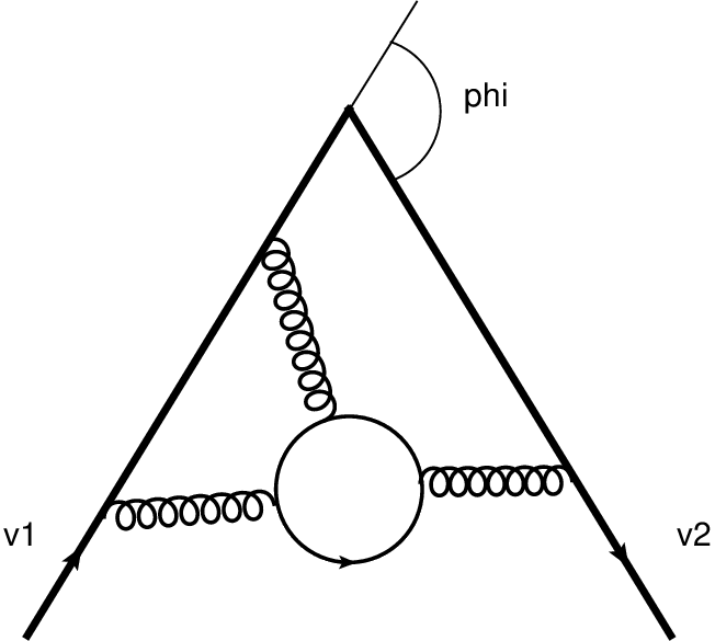
To compute the cusp anomalous dimension, we consider an integration contour formed by two segments along space-like directions and (with ), with cusp angle (cf. Fig. 1). In addition, we take the vectors and to be constant along the segments except the cusp point where they form an additional internal angle . The cusp anomalous dimension depends on the cusp angles and . It turns out to be convenient to introduce complex variables
| (2) |
The dependence of the cusp anomalous dimension on is polynomial. For simplicity of notation, let us set from now on, i.e. .
The two-loop results for the Wilson loop operators and in SYM are33 3 The supersymmetric results quoted here are valid in the DRED scheme, while formulas in QCD will be given in the scheme. See Appendix A of ref. [10] for a discussion of the scheme conversion up to two loops.
| (3) | ||||
| (4) |
where is the ’t Hooft coupling and
| (5) | ||||
Eq. (3) is due to the last ref. in [4], while to the best of our knowledge eq. (4) is new. Note that although each of the functions (5) has uniform weight , and , respectively, they produce a ‘weight drop’ contribution when evaluated at zero angle, , , and .
Interestingly, the cusp anomalous dimension for the bosonic Wilson loop in SYM differs only slightly from the supersymmetric one. Moreover, the function is related to a derivative of , if one considers and as independent variables,
| (6) |
Using relations (5), we can rewrite the known two-loop result for the QCD cusp anomalous dimension in a new way, in terms of the simple functions encountered in SYM,
| (7) | ||||
| (8) |
where the expansion parameter is , and are quadratic Casimirs of the gauge group in the fundamental and adjoint representation, respectively, is the number of quark flavours and .
3 Uniform weight functions and computation of the master integrals
Why should uniform weight functions play such an important role for the cusp anomalous dimension? In fact, the perturbative expansion of a cusped Wilson loop (1) gives rise to distinct Feynman integrals which are already very close to the definition of iterated integrals [11]. In the third reference of [5], this observation was used to give an algorithm for computing any Wilson line integral with an arbitrary number of propagator exchanges (but no internal vertices).44 4 A different computation of some of these integrals is discussed in [12]. For the full computation we require a larger class of integrals that includes graphs with interaction vertices. A method which exposes the weight properties of such integrals was proposed in [13], and we used it for our computation.
Since the three-loop cusp anomalous dimension does not receive nonplanar corrections, it can be expressed in terms of planar integrals only. We choose to perform the calculation in momentum space, using the heavy quark effective theory framework [3]. The integrals can all be parametrized as (with )
| (9) |
for certain choices of positive/negative integers . Applying the integral reduction algorithms [14], we found that 71 master integrals are required in total.55 5 A subset of these integrals that reduce to a one-loop triangle with -dependent indices was computed in ref. [16]. We then used the method proposed in ref. [13] to choose a convenient basis for the latter, denoted by . A distinguished feature of this basis is that the satisfy the differential equations of the form ()
| (10) |
with constant ( and independent) matrices . We see that eq. (10) has four regular singular points, . Due to the symmetry of the definition , only the first three are independent. They correspond, in turn, to the light-like limit (infinite angle), to the zero angle limit, and to the threshold limit. See ref. [5] for further discussion of these limits.
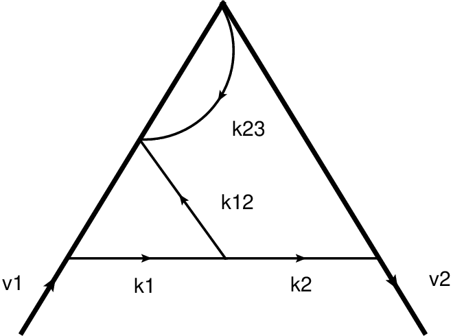
Solving (10) we use boundary conditions for at . All except one can be easily obtained from consistency conditions, i.e. absence of unphysical singularities, and the remaining constant can be found by comparing to refs. [17]. If follows immediately from (10) that the solution for in the from of expansion can be written in terms of harmonic polylogarithms [18]. In this way, we obtained an analytic answer in terms of uniform weight functions for all integrals required. As an example, we consider one of the master integrals
| (11) |
We performed numerical checks on all integrals using FIESTA [19], and analytically reproduced results for three-loop integrals known from the SYM computation [5]. More details will be discussed elsewhere.
4 Three-loop cusp anomalous dimension in QCD
To compute the cusp anomalous dimension, we started with the definition of the bosonic Wilson loop (1) in QCD, and generated all Feynman diagrams contributing to up to three loops, in an arbitrary covariant gauge. This was done with the help of the computer programs QGRAF and FORM [15]. The dependent contribution only comes from diagrams with quarks propagating inside the loops. They can be evaluated within dimensional regularization using standard methods, details will be given elsewhere.
The cusp anomalous dimension can be extracted from the divergent part of the one-particle irreducible vertex function of the heavy-to-heavy current [3] (e.g., the diagram in Fig. 1 without the external leg propagators),
| (12) |
In the scheme, the renormalization factor has the following structure
| (13) |
where the dependence only enters through the renormalised coupling constant [20], . As a non-trivial check of our calculation we verified that eq. (13) indeed reproduces the pole structure of at three loops.
At three loops, the cusp anomalous dimension has the following form by virtue of non-Abelian exponentiation,
| (14) |
For the dependent terms, we obtained the following results,
| (15) | ||||
with the functions , and given in eq. (5).
The following comments are in order. The leading term in (14) is in agreement with the known result [21]. The expressions for the coefficients and in the subleading terms are new ( can be obtained by generalizing the method of the last ref. of [3]).
As yet another check of our result, we can take the light-like limit of (14), where one expects [22] the behavior , with at three loops computed in refs. [23]. Again, we observed a perfect agreement for the dependent terms.
It is remarkable that despite the relative complexity of the Feynman integrals (9), the final expressions (15) are surprisingly simple! Moreover, they are expressed in terms of the same functions that appear in the SYM answer. It will be interesting to see whether this is also the case for the term. This calculation is work in progress.
5 Discussion
The simplicity of eqs. (15) suggests that there should be a simpler way of arriving at these results. Ignoring technical details such as the intrinsic renormalization of the Lagrangian and the associated function, morally speaking there should be a way of organizing the calculation in terms of manifestly finite integrals in four dimensions, as in ref. [24]. This would very likely require only a (simpler) subset of functions as compared to the calculation in dimensions.
A related comment is that when computing integrals via differential equations, usually one proceeds in a “bottom-up” approach: one starts with the integrals with few propagators, e.g. a tadpole integral, when proceeds with bubbles, and so on. Let us now imagine a scenario where, through some means, one knows the answer for SYM. The integrals required for SYM are typically the ones with maximal number of propagators, thanks to its good ultraviolet properties. In the traditional approach, one arrives at them only at the very end, and therefore they obviously contain a lot of information. Given this, it is interesting to ask whether one can use this information in a “top-down” approach, and how many of the master integrals required for QCD are determined by it.
Acknowledgments.
We wish to thank R. N. Lee for his help in using LiteRed, and K. G. Chetyrkin, M. Steinhauser and V. Smirnov for helpful conversations. We are also grateful to several institutes that have provided hospitality to some of us during scientific visits in the course of this work, namely IPhT Saclay, the Karlsruhe Institute of Technology (KIT), and the Institute for Advanced Study, Princeton. A.G.’s work was supported by RFBR grant 12-02-00106-a and by the Russian Ministry of Education and Science. J.M.H. is supported in part by the DOE grant DE-SC0009988 and by the Marvin L. Goldberger fund. G.P.K. is supported in part by the French National Agency for Research (ANR) under contract StrongInt (BLANC-SIMI-4-2011). P.M. was supported in part by the DFG through the SFB/TR 9 “Computational Particle Physics” and the EU Networks LHCPHENOnet PITN-GA-2010-264564 and HIGGSTOOLS PITN-GA-2012-316704.References
- [1] A. M. Polyakov, Nucl. Phys. B 164, (1980) 171; R. A. Brandt, F. Neri and M. Sato, Phys. Rev. D 24 (1981) 879.
- [2] G. P. Korchemsky and A. V. Radyushkin, Phys. Lett. B 171 (1986) 459; Phys. Lett. B 279 (1992) 359.
- [3] M. Neubert, Phys. Rept. 245 (1994) 259; A. V. Manohar and M. B. Wise, Camb. Monogr. Part. Phys. Nucl. Phys. Cosmol. 10 (2000) 1; A. G. Grozin, Springer Tracts Mod. Phys. 201 (2004) 1.
- [4] G. P. Korchemsky and A. V. Radyushkin, Nucl. Phys. B 283 (1987) 342; N. Kidonakis, Phys. Rev. Lett. 102 (2009) 232003; N. Drukker and V. Forini, JHEP 1106 (2011) 131.
- [5] D. Correa, J. Henn, J. Maldacena and A. Sever, JHEP 1205 (2012) 098; J. M. Henn and T. Huber, JHEP 1211 (2012) 058; J. M. Henn and T. Huber, JHEP 1309 (2013) 147.
- [6] J. M. Maldacena, Phys. Rev. Lett. 80 (1998) 4859; N. Drukker, D. J. Gross and H. Ooguri, Phys. Rev. D 60 (1999) 125006; V. Forini, JHEP 1011 (2010) 079.
- [7] D. Correa, J. Henn, J. Maldacena and A. Sever, JHEP 1206 (2012) 048; B. Fiol, B. Garolera and A. Lewkowycz, JHEP 1205 (2012) 093.
- [8] D. Correa, J. Maldacena and A. Sever, JHEP 1208 (2012) 134; N. Drukker, JHEP 1310, 135 (2013); N. Gromov and A. Sever, arXiv:1207.5489 [hep-th]; Z. Bajnok, J. Balog, D. H. Correa, Á. Hegedüs, F. I. Schaposnik Massolo and G. Zsolt Tóth, JHEP 1403 (2014) 056.
- [9] J. M. Henn, S. G. Naculich, H. J. Schnitzer and M. Spradlin, JHEP 1004 (2010) 038;
- [10] A. V. Belitsky, A. S. Gorsky and G. P. Korchemsky, Nucl. Phys. B 667 (2003) 3.
- [11] K. -T. Chen, Bull. Am. Math. Soc. 83 (1977) 831.
- [12] E. Gardi, talk at Loops and Legs 2014; L. Magnea, talk at Loops and Legs 2014.
- [13] J. M. Henn, Phys. Rev. Lett. 110 (2013) no. 25, 251601.
- [14] A. V. Smirnov, JHEP 0810 (2008) 107; R. N. Lee, arXiv:1212.2685 [hep-ph]; P. Marquard, D. Seidel, unpublished.
- [15] P. Nogueira, J. Comput. Phys. 105 (1993) 279; J. A. M. Vermaseren, math-ph/0010025.
- [16] A. G. Grozin and A. V. Kotikov, arXiv:1106.3912 [hep-ph].
- [17] A. G. Grozin, JHEP 0003 (2000) 013; K. G. Chetyrkin and A. G. Grozin, Nucl. Phys. B 666 (2003) 289.
- [18] E. Remiddi and J. A. M. Vermaseren, Int. J. Mod. Phys. A 15 (2000) 725; D. Maître, Comput. Phys. Commun. 174 (2006) 222.
- [19] A. V. Smirnov and M. N. Tentyukov, Comput. Phys. Commun. 180 (2009) 735.
- [20] T. van Ritbergen, J. A. M. Vermaseren and S. A. Larin, Phys. Lett. B 400 (1997) 379.
- [21] M. Beneke and V. M. Braun, Nucl. Phys. B 454 (1995) 253.
- [22] G. P. Korchemsky, Mod. Phys. Lett. A 4 (1989) 1257; G. P. Korchemsky and G. Marchesini, Nucl. Phys. B 406 (1993) 225.
- [23] A. Vogt, Phys. Lett. B 497 (2001) 228; C. F. Berger, Phys. Rev. D 66 (2002) 116002; S. Moch, J. A. M. Vermaseren and A. Vogt, Phys. Lett. B 625 (2005) 245.
- [24] S. Caron-Huot and J. M. Henn, JHEP 1406 (2014) 114.