跳到论文正文
W Papers独立论文阅读器 arXiv:1406.7623 论文正文 计算阅读时间 · 0%
引用这篇论文根据当前论文元数据生成,正式投稿前建议核对。


License: arXiv.org perpetual non-exclusive license
arXiv:1406.7623v1 [cs.IT] 30 Jun 2014

Transmit Designs for the MIMO Broadcast Channel with Statistical CSIThanks: Copyright (c) 2014 IEEE. Personal use of this material is permitted. However, permission to use this material for any other purposes must be obtained from the IEEE by sending a request to pubs-permissions@ieee.org.Thanks: Part of this paper was presented at IEEE International Conference on Communication (ICC’11), Kyoto, Japan, Jun. 2011. Thanks: The work of Y. Wu, S. Jin, and X. Gao was supported in part by National Natural Science Foundation of China under Grants 61320106003 and 61222102, the China High-Tech 863 Plan under Grant 2012AA01A506, National Science and Technology Major Project of China under Grants 2013ZX03003004 and 2014ZX03003006-003, the Program for Jiangsu Innovation Team, and the Supporting Program for New Century Excellent Talents in University. The work of Y. Wu was also supported by the Alexander von Humboldt Foundation. The work of M. R. McKay was supported by the Hong Kong Research Grants Council under grant number 616713. The work of C. Xiao was supported in part by National Science Foundation under Grants CCF-0915846 and ECCS-1231848. Part of this work was carried out while Y. Wu was a visiting scholar at Missouri University of Science and Technology. Thanks: Y. Wu was with the National Mobile Communication Research Laboratory, Southeast University, Nanjing, 210096, P. R. China (email: ypwu@seu.edu.cn). Y. Wu is now with Institute for Digital Communications, Universita¨\ddot{a}t Erlangen-Nu¨\ddot{u}rnberg, Cauerstrasse 7, D-91058 Erlangen, Germany (email: yongpeng.wu@lnt.de). Thanks: S. Jin and X. Gao are with the National Mobile Communication Research Laboratory, Southeast University, Nanjing, 210096, P. R. China (email: jinshi@seu.edu.cn; xqgao@seu.edu.cn;). Thanks: M. R. McKay is with Department of Electrical and Computer Engineering, Hong Kong University of Science and Technology, Clear Water Bay, Kowloon, Hong Kong, (email: eemckay@ust.hk).Thanks: C. Xiao is with Department of Electrical and Computer Engineering, Missouri University of Science and Technology, Rolla, MO 65409, USA, (email: xiaoc@mst.edu).

Yongpeng Wu    Shi Jin    Xiqi Gao Affiliation: Matthew R. McKay, , and Chengshan Xiao, .
Abstract

We investigate the multiple-input multiple-output broadcast channel with statistical channel state information available at the transmitter. The so-called linear assignment operation is employed, and necessary conditions are derived for the optimal transmit design under general fading conditions. Based on this, we introduce an iterative algorithm to maximize the linear assignment weighted sum-rate by applying a gradient descent method. To reduce complexity, we derive an upper bound of the linear assignment achievable rate of each receiver, from which a simplified closed-form expression for a near-optimal linear assignment matrix is derived. This reveals an interesting construction analogous to that of dirty-paper coding. In light of this, a low complexity transmission scheme is provided. Numerical examples illustrate the significant performance of the proposed low complexity scheme.

Index Terms: 
Broadcast channel, multiple-input multiple-output, statistical CSI

I Introduction

The multiple-input multiple-output (MIMO) broadcast channel (BC) with Gaussian noise has attracted tremendous research interest in recent years. Dirty paper coding (DPC) has been proved to achieve the capacity region of this channel [1], whereas various linear precoding techniques have also been developed to reduce complexity (see, e.g., [2, 3, 4, 5, 6, 7]). Much current work dealing with the MIMO BC model assume that instantaneous channel state information (CSI) is available at both the transmitter and receivers, in order to fully capitalize on the spatial multiplexing advantages of the MIMO transmission. Whilst this assumption may be plausible for fixed or low mobility applications for which the channel realizations change slowly enough to be monitored at the transmitter (e.g., via a feedback link or by exploiting channel reciprocity), for other applications it becomes less feasible. In particular, as mobility increases, the channel fluctuations begin to vary more rapidly, and tracking these gains accurately at the transmitter becomes problematic.

For mobile applications, an alternative approach is to exploit statistical CSI at the transmitter [8, 9, 10, 11, 12, 14, 13, 15]; a technique which has drawn much attention in MIMO system design recently [16]. Compared with instantaneous CSI, the statistical parameters typically vary over a much longer time window, and therefore can be monitored more easily at the transmitter. With statistical CSI at the transmitter, an important problem is to understand the information-theoretic limits of the MIMO BC model. In the special case of “more capable” channels, where the power of signals to each receiver can be ordered, the ergodic capacity region was analyzed in [17], developing upon earlier work [28, 19]. For the fading single-input single-output (SISO) BC model, an achievable inner bound of the ergodic capacity region was proposed in [20]. This work was extended to the fading multiple-input single-output (MISO) BC model in [21], where the distributions of the fading coefficients were assumed isotropic and the ergodic capacity region was proved to collapse to that of the fading SISO BC model. Zhang et al. [22] examined an outage achievable rate region for the fading single-input multiple-output (SIMO) and MISO BC models. Very recently, simple linear precoding designs for some special MISO BC models were proposed in [23, 24].

Despite significant advances as described above, for the fading MIMO BC model, the capacity region remains unknown. To simplify the problem, a so-called linear assignment operation was proposed in [25]. Also, a linear assignment capacity was defined in [25] which, to the best of our knowledge, is the most systematic result revealing the information-theoretic limits of the fading MIMO BC model so far. However, comprehensive and explicit transmit designs based on this linear assignment operation were not given in [25] and are still missing in general.

In this paper, starting with the definition of the linear assignment capacity in [25], we consider the transmit design problem aimed at optimizing the linear assignment weighted sum-rate (LAWSR) of the fading MIMO BC model with statistical CSI at the transmitter. Based on an exact expression of the LAWSR, we reveal two key elements that need to be properly designed: 1) The linear assignment matrices; 2) The precoding matrices of the receivers.

We make the following key contributions:

  1. 1)

    We establish necessary conditions for the optimal linear assignment matrices and precoding matrices. Accordingly, the joint design of these can be formulated as a multidimensional optimization problem, which is solved by an alternating optimization method with a gradient descent update.

  2. 2)

    For the linear assignment matrix of each receiver, we provide a heuristic design with reduced computational complexity. This is done by rewriting the expression for the linear assignment achievable rate (LAAR) of each receiver as a difference of two terms, and applying Jensen’s inequality to each. This operation results in similar “bounding errors” for each of the two terms, but we prove it still leads to a strict upper bound of LAAR, which turns out to be fairly tight.

  3. 3)

    The derived upper bound motivates the establishment of a near-optimal construction for the linear assignment matrix to maximize the LAAR. Based on this construction, a simplified closed-form expression for the linear assignment matrix via second-order statistics of the CSI is obtained. This expression resembles the DPC structure, where the interference signal power has no impact on determining the linear assignment matrix. Moreover, for the design based on the derived upper bound and the simplified linear assignment matrix, it is shown that an interference elimination effect analogous to that of DPC transmission with instantaneous CSI exists. In light of this, a low complexity algorithm without numerical averaging is proposed to design the precoding matrices.

  4. 4)

    We reveal that if all the channels of the receivers are independent and identically distributed (i.i.d.) fading, the time division multiple access (TDMA) transmission is optimal. Also, we reveal that if the transmitter has only one antenna, the opportunistic scheduling transmission based on the statistical CSI is optimal11 1 For the single antenna i.i.d. case, the TDMA transmission and the opportunistic scheduling transmission are equivalent..

Numerical results are presented to examine the proposed transmission designs. These indicate that the proposed designs perform close to the no-interference upper bound of the MIMO BC with statistical CSI [25], and achieve significant performance gains compared to the TDMA transmission in various scenarios.

The reminder of the paper is organized as follows. Section II describes the fading MIMO BC model under consideration. In Section III, we establish necessary conditions of the optimal linear assignment matrices and precoding matrices for all the receivers, and propose an iterative algorithm to search for the optimal solution. In Section IV, we derive an upper bound of the LAAR of each receiver, based on which we investigate low complexity transmit designs. Numerical results are provided in Section V and the main results are summarized in Section VI. Main mathematical proofs have been placed in the Appendices.

The following notation is adopted throughout the paper: Vectors are represented as columns and are denoted in lower case bold-face, and matrices are represented in upper case bold-face. The superscripts (⋅)T(\cdot)^{T}, (⋅)∗(\cdot)^{*}, and (⋅)H(\cdot)^{H} stand for the matrix transpose, conjugate and conjugate-transpose operations, respectively. We use det⁡(⋅)\rm{det}(\cdot) and tr⁡(⋅)\rm{tr}(\cdot) to denote the matrix determinant and trace operations respectively, and 𝐀−1{\bf{A}}^{-1} denote the inverse of matrix 𝐀\bf{A}. ∘\circ denotes the Hadamard product of two matrices. 𝐀⪰𝟎\mathbf{A}\succeq\mathbf{0} means that 𝐀\mathbf{A} is Hermitian positive semi-definite, and 𝐀≻𝟎\mathbf{A}\succ\mathbf{0} means that 𝐀\mathbf{A} is Hermitian positive definite. ‖𝐗‖F\left\|{\mathbf{X}}\right\|_{F} denotes the Frobenius norm of matrix 𝐗\mathbf{X}. The M×MM\times M identity matrix is denoted by 𝐈M{\bf{I}}_{M}, and the all-zero matrix is denoted by 𝟎\bf{0}. The complex number field is represented by ℂ\mathbb{C}, and E⁡[⋅]E\left[\cdot\right] evaluates the expectation of all the random variables within the bracket.

II System Model

Consider a fading MIMO BC scenario, where the transmitter has NtN_{t} antennas, while each of the LL receivers has NrN_{r} antennas. The received vector for the ll-th receiver can be written as

𝐲l=𝐇l​𝐱T+𝐳l{\bf{y}}_{l}={\bf{H}}_{l}{\bf{x}}_{T}+{\bf{z}}_{l} (1)

where 𝐱T∈ℂNt×1{\bf{x}}_{T}\in{\mathbb{C}}^{{N_{t}\times 1}} is the transmitted vector designed to meet the power constraint

E⁡[tr⁡(𝐱T​𝐱TH)]≤P.E\left[{{\rm{tr}}\left({{\bf{x}}_{T}{\bf{x}}_{T}^{H}}\right)}\right]\leq P. (2)

𝐳l∈ℂNr×1{\bf{z}}_{l}\in{\mathbb{C}}^{{N_{r}\times 1}} contains circularly symmetric complex Gaussian noise with zero-mean and covariance E⁡[𝐳l​𝐳lH]E\left[{{\bf{z}}_{l}{\bf{z}}_{l}^{H}}\right] =N0​𝐈Nr=N_{0}{\bf{I}}_{N_{r}}, and 𝐇l∈ℂNr×Nt{\bf{H}}_{l}\in{\mathbb{C}}^{{N_{r}\times N_{t}}} is a random channel matrix. The channels are assumed independent across ll, i.e., for different receivers. Moreover, the ll-th receiver is assumed to perfectly estimate its own channel matrix, 𝐇l{\bf{H}}_{l}, whilst the transmitter only knows statistical CSI22 2 It is noted that throughout this paper, we make no assumption on the distribution of 𝐇l\mathbf{H}_{l}, beyond it having finite energy. for each receiver.

Here, the transmitted signal 𝐱T{\bf{x}}_{T} in (1) is constructed as 𝐱T=∑l=1L𝐱l{\bf{x}}_{T}=\sum\nolimits_{l=1}^{L}{{\bf{x}}_{l}}, where 𝐱l{\bf{x}}_{l} contains the transmitted signal destined for the ll-th receiver with the covariance matrix 𝚺l=E⁡[𝐱l​𝐱lH]{\bf{\Sigma}}_{l}=E\left[{{\bf{x}}_{l}{\bf{x}}_{l}^{H}}\right]. Similar to [25], we assume that 𝚺l{\bf{\Sigma}}_{l} is nonsingular. Moreover, we follow [25] to assume that the transmitter generates the transmitted data for each user in ascending order. Thus, when designing the transmitted signal for the ll-th receiver, the transmitter possesses the full non-causal knowledge of the transmitted codewords for the receivers 1,2,⋯,l−11,2,\cdots,l-1. To this end, we reexpress (1) as

𝐲l=𝐇l​(𝐱l+𝐬l)+𝐇l​∑t=l+1L𝐱t+𝐳l{\mathbf{y}}_{l}={\mathbf{H}}_{l}\left({{\mathbf{x}}_{l}+\mathbf{s}_{l}}\right)+{\mathbf{H}}_{l}\sum\limits_{t=l+1}^{L}{{\mathbf{x}}_{t}}+{\mathbf{z}}_{l} (3)

where 𝐬l=∑t=1l−1𝐱t\mathbf{s}_{l}=\sum\limits_{t=1}^{l-1}{{\mathbf{x}}_{t}}. In the absence of the instantaneous CSI at the transmitter, the pair (𝐲l,𝐇l)(\mathbf{y}_{l},\mathbf{H}_{l}) constitutes the channel output. The channel transition probability Pr[𝐲l,𝐇l|𝐱l,𝐬l]{\rm{Pr}}[\mathbf{y}_{l},\mathbf{H}_{l}|\mathbf{x}_{l},\mathbf{s}_{l}] of the fading MIMO BC model in (3) is a function of the transmitted signal 𝐱l{\mathbf{x}}_{l}, the channel matrix 𝐇l\mathbf{H}_{l}, and the state of the non-causally known interference 𝐬l\mathbf{s}_{l}, which is an instance of the general class of side-information channels [26, 27]. Hence the capacity for the ll-th receiver in model (3) is defined as

Cl=supPr[𝐮l|𝐬l],fl(.){I(𝐮l;𝐲l,𝐇l)−I(𝐮l;𝐬l)}C_{l}=\mathop{\sup}\limits_{\Pr[{\mathbf{u}}_{l}\left|{\mathbf{s}_{l}}\right.],\,f_{l}\left(.\right)}\left\{{I\left({{\mathbf{u}}_{l};{\mathbf{y}_{l}},{\mathbf{H}_{l}}}\right)-I\left({{\mathbf{u}_{l}};{\mathbf{s}_{l}}}\right)}\right\} (4)

where 𝐮l{\mathbf{u}_{l}} is an auxiliary random vector with the conditional distribution Pr[𝐮l|𝐬l]\Pr[{\mathbf{u}_{l}}\left|{\mathbf{s}_{l}}\right.] and fl​(⋅)f_{l}\left(\cdot\right) is a deterministic function which constructs the transmitted signal as 𝐱l=fl​(𝐮l,𝐬l){\mathbf{x}_{l}}=f_{l}({\mathbf{u}_{l},\mathbf{s}_{l}}) and satisfies E⁡[fl​(𝐮l,𝐬l)​fl​(𝐮l,𝐬l)H]=𝚺lE\left[{f_{l}({\mathbf{u}_{l},\mathbf{s}_{l}})}{f_{l}({\mathbf{u}_{l},\mathbf{s}_{l}})}^{H}\right]={{\bf{\Sigma}}_{l}}. We note that for any particular choice of Pr[𝐮l|𝐬l]\Pr[{\mathbf{u}_{l}}\left|{\mathbf{s}_{l}}\right.] and fl​(⋅)f_{l}\left(\cdot\right), expression (4) becomes an achievable transmission rate.

The maximum achievable rate of the fading MIMO BC model in (4) remains an open problem. However, by generating 𝐱l=fl​(𝐮l,𝐬l)=𝐮l−𝐅l​𝐬l\mathbf{x}_{l}=f_{l}({\mathbf{u}_{l},\mathbf{s}_{l}})={\mathbf{u}_{l}}-\mathbf{F}_{l}\mathbf{s}_{l}, where 𝐅l{\mathbf{F}}_{l} represents the Nt×NtN_{t}\times N_{t} constant linear assignment matrix, we have an achievable transmission rate

RLA,l=sup𝐅l{Rl}R_{{\rm{LA}},\,l}=\mathop{\sup}\limits_{\mathbf{F}_{l}}\left\{R_{l}\right\} (5)

where

Rl=supPr[𝐮l|𝐬l]{(I(𝐮l;𝐲l,𝐇l)−I(𝐮l;𝐬l))|fl(𝐮l,𝐬l)=𝐮l−𝐅l𝐬l}.\begin{array}[]{l}R_{l}=\\ \hskip-5.69046pt\mathop{\sup}\limits_{\Pr[{\mathbf{u}}_{l}\left|{\mathbf{s}_{l}}\right.]}\left\{{\left(I\left({{\mathbf{u}}_{l};{\mathbf{y}_{l}},{\mathbf{H}_{l}}}\right)-I\left({{\mathbf{u}_{l}};{\mathbf{s}_{l}}}\right)\right)|{f_{l}({\mathbf{u}_{l},\mathbf{s}_{l}})={\mathbf{u}_{l}}-\mathbf{F}_{l}\mathbf{s}_{l}}}\right\}.\end{array} (6)

Given any fixed linear assignment matrix 𝐅l\mathbf{F}_{l}, it was proved in [25, Theorem 1] that the maximum rate in (6) is achieved by choosing 𝐱l\mathbf{x}_{l} to be jointly Gaussian with 𝐬l\mathbf{s}_{l}, which in turn determines the conditional distribution Pr[𝐮l|𝐬l]\Pr[{\mathbf{u}_{l}}\left|{\mathbf{s}_{l}}\right.] as follows [25]

Pr[𝐮l|𝐬l]=1det(π​𝚺𝐮l,𝐬l)​exp⁡(−(𝐮l−𝐉l​𝐬l)H​𝚺𝐮l,𝐬l−1​(𝐮l−𝐉l​𝐬l))\begin{array}[]{l}\Pr\left[{{\bf{u}}_{l}\left|{{\bf{s}}_{l}}\right.}\right]=\\ \qquad\frac{1}{{\sqrt{\det\left({\pi{\bm{\Sigma}}_{{\bf{u}}_{l},{\bf{s}}_{l}}}\right)}}}\exp\left({-\left({{\bf{u}}_{l}-{\mathbf{J}_{l}\bf{s}}_{l}}\right)^{H}{\bm{\Sigma}}_{{\bf{u}}_{l},{\bf{s}}_{l}}^{-1}\left({{\bf{u}}_{l}-{\mathbf{J}_{l}\bf{s}}_{l}}\right)}\right)\end{array} (7)

where

𝐉l=(𝐅l​𝚺𝐬l+𝚺𝐱l,𝐬lH)​𝚺𝐬l−1\mathbf{J}_{l}=\left({{\mathbf{F}_{l}\bf{\Sigma}}_{{\bf{s}}_{l}}+{\bm{\Sigma}}_{{\bf{x}}_{l},{\bf{s}}_{l}}^{H}}\right){\bm{\Sigma}}_{{\bf{s}}_{l}}^{-1} (8)

and

𝚺𝐮l,𝐬l=(𝐅l​𝚺𝐬l​𝐅lH+𝐅l​𝚺𝐱l,𝐬l+𝚺𝐱l,𝐬lH​𝐅lH+𝚺𝐱l)−(𝐅l​𝚺𝐬l+𝚺𝐱l,𝐬lH)​𝚺𝐬l−1​(𝐅l​𝚺𝐬l+𝚺𝐱l,𝐬lH)H\begin{array}[]{l}{\bf{\Sigma}}_{{\bf{u}}_{l},{{\bf{s}}_{l}}}=\left({{\mathbf{F}_{l}\bf{\Sigma}}_{{\bf{s}}_{l}}\mathbf{F}_{l}^{H}+{\mathbf{F}_{l}\bf{\Sigma}}_{{\bf{x}}_{l},{\bf{s}}_{l}}+{\bf{\Sigma}}_{{\bf{x}}_{l},{\bf{s}}_{l}}^{H}\mathbf{F}_{l}^{H}+{\bf{\Sigma}}_{{\bf{x}}_{l}}}\right)\\ \hskip 56.9055pt-\left({\mathbf{F}_{l}{\bf{\Sigma}}_{{\bf{s}}_{l}}+{\bf{\Sigma}}_{{\bf{x}}_{l},{\bf{s}}_{l}}^{H}}\right){\bf{\Sigma}}_{{\bf{s}}_{l}}^{-1}\left({\mathbf{F}_{l}{\bf{{\bm{\Sigma}}}}_{{\bf{s}}_{l}}+{\bf{\Sigma}}_{{\bf{x}}_{l},{\bf{s}}_{l}}^{H}}\right)^{H}\end{array} (9)

in which 𝚺𝐱l{\bf{\Sigma}}_{{\bf{x}}_{l}}, 𝚺𝐬l{\bf{\Sigma}}_{{\bf{s}}_{l}}, and 𝚺𝐱l,𝐬l{\bm{\Sigma}}_{{\bf{x}}_{l},{\bf{s}}_{l}} denotes the covariance matrix of 𝐱l\mathbf{x}_{l}, the covariance matrix of 𝐬l\mathbf{s}_{l}, and the cross-covariance matrix of 𝐱l\mathbf{x}_{l} and 𝐬l\mathbf{s}_{l}, respectively. Then, the achievable transmission rate in (5) under the linear assignment operation fl​(𝐮l,𝐬l)=𝐮l−𝐅l​𝐬lf_{l}\left({\mathbf{u}_{l}},{\mathbf{s}_{l}}\right)=\mathbf{u}_{l}-\mathbf{F}_{l}\mathbf{s}_{l} and the corresponding conditional distribution in (7) is defined as the linear assignment capacity [25]. Furthermore, it was proved in [25, Theorem 2] that the linear assignment capacity region of model (1) is found by choosing the transmitted vector 𝐱l\mathbf{x}_{l} independent33 3 It should be noted here we do not require that for a given user ll, the maximum value in (5) must choose 𝐱l\mathbf{x}_{l} to be independent of 𝐬l\mathbf{s}_{l}. Instead, the conclusion in [25, Theorem 2] indicates that by replacing the entire given signal set 𝐱l\mathbf{x}_{l}, l=1,2,⋯,Ll=1,2,\cdots,L, which may not be independent of the entire interference set 𝐬l\mathbf{s}_{l}, l=1,2,⋯,Ll=1,2,\cdots,L (corresponding to some set of points on the linear assignment capacity region), to two independent sets 𝐱~l\mathbf{\widetilde{x}}_{l}, l=1,2,⋯,Ll=1,2,\cdots,L and 𝐬~l\mathbf{\widetilde{s}}_{l}, l=1,2,⋯,Ll=1,2,\cdots,L, the entire linear assignment capacity region can be exhausted. For details, refer to Appendix V in [25]. of the interference vector 𝐬l\mathbf{s}_{l}, l=1,2,⋯,Ll=1,2,\cdots,L. In this case, we have 𝚺𝐱l=𝚺l{\bf{\Sigma}}_{{\bf{x}}_{l}}={\bf{\Sigma}}_{l}, 𝚺𝐬l=𝚺S,l=∑t=1l−1𝚺t{\bf{\Sigma}}_{{\bf{s}}_{l}}=\mathbf{\Sigma}_{S,\,l}=\sum\nolimits_{t=1}^{l-1}{\bf{\Sigma}}_{t}, 𝚺𝐱l,𝐬l=𝟎{\bm{\Sigma}}_{{\bf{x}}_{l},{\bf{s}}_{l}}=\mathbf{0}, and the covariance matrix of the transmitted signal 𝐱T{\bf{x}}_{T} can be expressed as 𝚺T=E⁡[𝐱T​𝐱TH]=∑l=1L𝚺l{\bm{\Sigma}}_{T}=E\left[{{\bf{x}}_{T}{\bf{x}}_{T}^{H}}\right]=\sum\nolimits_{l=1}^{L}{{\bm{\Sigma}}_{l}}. The transmitter is subject to an average power constraint PP, which implies tr⁡(𝚺T)≤P{\rm{tr}}\left({{\bm{\Sigma}}_{T}}\right)\leq P. Also, the conditional distribution Pr[𝐮l|𝐬l]\Pr[{\mathbf{u}_{l}}\left|{\mathbf{s}_{l}}\right.] in (7) reduces to

Pr[𝐮l|𝐬l]=1det(π​𝚺l)​exp⁡(−(𝐮l−𝐅l​𝐬l)H​𝚺l−1​(𝐮l−𝐅l​𝐬l)).\begin{array}[]{l}\Pr\left[{{\bf{u}}_{l}\left|{{\bf{s}}_{l}}\right.}\right]=\\ \quad\frac{1}{{\sqrt{\det\left({\pi{\bm{\Sigma}}_{l}}\right)}}}\exp\left({-\left({{\bf{u}}_{l}-{\mathbf{F}_{l}\bf{s}}_{l}}\right)^{H}{\bm{\Sigma}}_{l}^{-1}\left({{\bf{u}}_{l}-{\mathbf{F}_{l}\bf{s}}_{l}}\right)}\right).\end{array} (10)

Then, by adapting the LAAR expression in [25, Eq. (35)] to complex channels, the LAAR of the ll-th receiver in (6) can be written as

Rl=log2det(𝚺𝐮l,𝐬l)−E[log2det(𝚺𝐮l,𝐲l|𝐇l(𝐇l))]R_{l}=\log_{2}\det\left({{\bf{\Sigma}}_{{\mathbf{u}_{l}},{\mathbf{s}_{l}}}}\right)-E\left[{\log_{2}\det\left({\bf{\Sigma}}_{{\mathbf{u}_{l}},\,{\mathbf{y}_{l}}\left|{{\mathbf{H}_{l}}}\right.}\left({\mathbf{H}_{l}}\right)\right)}\right]\\ (11)

where

𝚺𝐮l,𝐲l|𝐇l(𝐇l)=(𝐅l𝚺𝐬l𝐅lH+𝐅l𝚺𝐱l,𝐬l+𝚺𝐱l,𝐬lH𝐅lH+𝚺𝐱l)−[(𝐅l​𝚺𝐬l+𝐅l​𝚺𝐱l,𝐬l+𝚺𝐱l,𝐬lH+𝚺𝐱l)​𝐇lH]×[𝐇l​(𝚺𝐬l+𝚺𝐱l+𝚺𝐱l,𝐬l+𝚺𝐱l,𝐬lH)​𝐇lH+𝚺Z,l​(𝐇l)]−1×[(𝐅l​𝚺𝐬l+𝐅l​𝚺𝐱l,𝐬l+𝚺𝐱l,𝐬lH+𝚺𝐱l)​𝐇lH]H\begin{array}[]{l}{\bf{\Sigma}}_{{\bf{u}}_{l},\,{\bf{y}}_{l}\left|{{\bf{H}}_{l}}\right.}\left({{\bf{H}}_{l}}\right)\!=\!\left({\mathbf{F}_{l}{\bm{\Sigma}}_{{\bf{s}}_{l}}\mathbf{F}_{l}^{H}\!+\!\mathbf{F}_{l}{\bm{\Sigma}}_{{\bf{x}}_{l},{\bf{s}}_{l}}\!+\!{\bm{\Sigma}}_{{\bf{x}}_{l},{\bf{s}}_{l}}^{H}\mathbf{F}_{l}^{H}\!+\!{\bm{\Sigma}}_{{\bf{x}}_{l}}}\right)\\ \hskip 28.45274pt-\left[{\left({\mathbf{F}_{l}{\bm{\Sigma}}_{{\bf{s}}_{l}}+\mathbf{F}_{l}{\bm{\Sigma}}_{{\bf{x}}_{l},{\bf{s}}_{l}}\!+\!{\bm{\Sigma}}_{{\bf{x}}_{l},{\bf{s}}_{l}}^{H}\!+\!{\bm{\Sigma}}_{{\bf{x}}_{l}}}\right){\bf{H}}_{l}^{H}}\right]\\ \times\left[{{\bf{H}}_{l}\left({{\bm{\Sigma}}_{{\bf{s}}_{l}}+{\bm{\Sigma}}_{{\bf{x}}_{l}}+{\bm{\Sigma}}_{{\bf{x}}_{l},{\bf{s}}_{l}}+{\bm{\Sigma}}_{{\bf{x}}_{l},{\bf{s}}_{l}}^{H}}\right){\bf{H}}_{l}^{H}\!+\!{\bm{\Sigma}}_{Z,l}\left({{\bf{H}}_{l}}\right)}\right]^{-1}\\ \hskip 14.22636pt\times\left[{\left(\mathbf{F}_{l}{\bm{\Sigma}}_{{\bf{s}}_{l}}+\mathbf{F}_{l}{\bm{\Sigma}}_{{\bf{x}}_{l},{\bf{s}}_{l}}+{\bm{\Sigma}}_{{\bf{x}}_{l},{\bf{s}}_{l}}^{H}+{\bm{\Sigma}}_{{\bf{x}}_{l}}\right){\bf{H}}_{l}^{H}}\right]^{H}\\ \end{array} (12)

in which 𝚺Z,l​(𝐇l)=𝐇l​(∑t=l+1L𝚺t)​𝐇lH+N0​𝐈Nr\mathbf{\Sigma}_{Z,\,l}(\mathbf{H}_{l})=\mathbf{H}_{l}\left(\sum\nolimits_{t=l+1}^{L}{\bf{\Sigma}}_{t}\right)\mathbf{H}_{l}^{H}+N_{0}\mathbf{I}_{N_{r}}. Since 𝐱l\mathbf{x}_{l} and 𝐬l\mathbf{s}_{l} are independent (𝚺𝐱l,𝐬l=𝟎{\bm{\Sigma}}_{{\bf{x}}_{l},{\bf{s}}_{l}}=\mathbf{0}), (9) and (12) can be simplified as follows

𝚺𝐮l,𝐬l=𝚺l{\bm{\Sigma}}_{{\mathbf{u}_{l}},{\mathbf{s}_{l}}}={\bf{\Sigma}}_{l} (13)
𝚺𝐮l,𝐲l|𝐇l(𝐇l)=𝐂l−𝐀l​𝐇lH​[𝐇l​𝐁l​𝐇lH+𝚺Z,l​(𝐇l)]−1​𝐇l​𝐀lH\begin{array}[]{l}{\bf{\Sigma}}_{{\mathbf{u}_{l}},\,{\mathbf{y}_{l}}\left|{{\mathbf{H}_{l}}}\right.}\left({\mathbf{H}_{l}}\right)=\\ \hskip 28.45274pt{\mathbf{C}_{l}}-{\mathbf{A}_{l}\mathbf{H}_{l}^{H}}\left[{{\mathbf{H}_{l}\mathbf{B}_{l}{\mathbf{H}_{l}^{H}}}+\mathbf{\Sigma}_{Z,\,l}(\mathbf{H}_{l})}\right]^{-1}{\mathbf{H}_{l}}\mathbf{A}_{l}^{H}\\ \end{array} (14)

where 𝐀l=𝐅l​𝚺S,l+𝚺l{\bf{A}}_{l}={\bf{F}}_{l}\mathbf{\Sigma}_{S,\,l}+{\bf{\Sigma}}_{l}, 𝐁l=𝚺S,l+𝚺l{\bf{B}}_{l}=\mathbf{\Sigma}_{S,\,l}+{\bf{\Sigma}}_{l}, and 𝐂l=𝐅l​𝚺S,l​𝐅lH+𝚺l{\bf{C}}_{l}={{\bf{F}}_{l}\mathbf{\Sigma}_{S,\,l}{\bf{F}}_{l}^{H}}+{\bf{\Sigma}}_{l}.

Here we present the encoding and decoding process to achieve the linear assignment achievable rate in (11).

Encoding process at the transmitter:

  1. 1)

    First select a transmitted signal 𝐱1\mathbf{x}_{1} for receiver 1.

  2. 2)

    Generate en​I​(𝐮2,𝐲2,𝐇2)e^{nI(\mathbf{u}_{2};\mathbf{y}_{2},\mathbf{H}_{2})} independent sequences.

  3. 3)

    Distribute these sequences into the en​R2e^{nR_{2}} bin codebook uniformly.

  4. 4)

    Given the non-causally known interference 𝐬2=𝐱1\mathbf{s}_{2}=\mathbf{x}_{1} and the message W2=kW_{2}=k for receiver 2, look for a joint typical pair [28] (𝐮2\mathbf{u}_{2}, 𝐬2\mathbf{s}_{2}) among the sequences in bin kk.

  5. 5)

    The signal 𝐱2{\bf{x}}_{2} for receiver 22 is constructed using the linear assignment operation 𝐱2=𝐮2−𝐅2​𝐬2\mathbf{x}_{2}=\mathbf{u}_{2}-\mathbf{F}_{2}\mathbf{s}_{2}.

  6. 6)

    The signal 𝐱l\mathbf{x}_{l} for receiver ll is constructed in a similar manner above. The signal 𝐬l=𝐱1+𝐱2+⋯+𝐱l−1{\bf{s}}_{l}={\bf{x}}_{1}+{\bf{x}}_{2}+\cdots+{\bf{x}}_{{l-1}} is regarded as non-causally known interference. This process continues to the LL-th receiver.

Decoding process at receiver ll:

  1. 1)

    For the received signal 𝐲l\mathbf{y}_{l}, look for a joint typical pair (𝐮l\mathbf{u}_{l}, 𝐲l\mathbf{y}_{l}, 𝐇l\mathbf{H}_{l}) among the sequences in the codebook.

  2. 2)

    Declare an error when more than one joint typical pairs (𝐮l\mathbf{u}_{l}, 𝐲l\mathbf{y}_{l}, 𝐇l\mathbf{H}_{l}) are found. Also, declare an error when no joint typical pair (𝐮l\mathbf{u}_{l}, 𝐲l\mathbf{y}_{l}, 𝐇l\mathbf{H}_{l}) is found.

  3. 3)

    Set the estimate W^l\widehat{W}_{l} equal to the index of the bin containing this sequence 𝐮l\mathbf{u}_{l}.

With the LAAR in (11), the LAWSR of model (1) is given by

Rsumw=∑l=1Lμl​RlR_{\rm{sum}}^{\rm{w}}=\sum\limits_{l=1}^{L}{\mu_{l}R_{l}} (15)

where RlR_{l} is evaluated in (11) and μl\mu_{l}, l=1,2,⋯,Ll=1,2,\cdots,L are nonnegative weights44 4 In a practical communication system, these weights can be determined according to different service requirements for different users. satisfying ∑l=1Lμl=L\sum\nolimits_{l=1}^{L}{\mu_{l}}=L. The sequel resorts to develop a transmit design of 𝐅l\mathbf{F}_{l} and 𝚺l\mathbf{\Sigma}_{l}, l=1,2,⋯,Ll=1,2,\cdots,L, under the constraint tr⁡(∑l=1L𝚺l)≤P{\rm{tr}}\left(\sum\nolimits_{l=1}^{L}{{\bf{\Sigma}}_{l}}\right)\leq P, by maximizing the LAWSR in (15).

III Transmit Design for Maximizing the LAWSR

In this section, we investigate the transmit design to maximize the LAWSR in (15). We begin by establishing necessary conditions that the optimal 𝐅l\mathbf{F}_{l} and 𝚺l\mathbf{\Sigma}_{l} must satisfy. Then, an algorithm is developed to optimize 𝐅l\mathbf{F}_{l} and 𝚺l\mathbf{\Sigma}_{l} iteratively.

III-A Necessary Conditions for the Optimal Design

From (15), we know that the objective function RsumwR_{\rm{sum}}^{\rm{w}} is a non-convex function of the matrices 𝐅l\mathbf{F}_{l} and 𝚺l\mathbf{\Sigma}_{l}, l=1,2,⋯,Ll=1,2,\cdots,L. Thus, we obtain a set of necessary conditions for the optimal linear assignment matrices and precoding matrices below.

Theorem 1

The optimal transmit design, which maximizes the LAWSR in (15), satisfies the following conditions:

−μllog2eE𝐇l[𝚺𝐮l|𝐲l,𝐇l(𝐇l)−1(𝐅l−𝐓l(𝐇l))𝚺S,l]=𝟎,l=1,2,⋯,L\begin{array}[]{l}\hskip-5.69046pt-\mu_{l}\log_{2}eE_{{\bf{H}}_{l}}\left[{\bm{\Sigma}_{{\bf{u}}_{l}\left|{{\bf{y}}_{l},\,{\bf{H}}_{l}}\right.}\left({{\bf{H}}_{l}}\right)^{-1}\left({\bf{F}}_{l}-{\bf{T}}_{l}\left({{\bf{H}}_{l}}\right)\right)}{\bm{\Sigma}}_{S,\,l}\right]=\mathbf{0},\\ \hskip 170.71652ptl=1,2,\cdots,L\end{array} (16)
𝚺l=𝐏l𝐏lH,l=1,2,⋯,L\bm{\Sigma}_{l}={\bf{P}}_{l}{\bf{P}}_{l}^{H},\quad l=1,2,\cdots,L (17)
(𝐏tH)−1−log2e[∑l=1t−1μlE𝐇l[𝐆1,l(𝐇l)]+μtE𝐇t[𝐆2,t(𝐇t)]+∑l=t+1LμlE𝐇l[𝐆3,l(𝐇l)]]𝐏t=θ𝐏t,t=1,2,⋯,L\begin{array}[]{l}\hskip-5.69046pt\left({{\bf{P}}_{t}^{H}}\right)^{-1}\!-\!\log_{2}e\,\left[\sum\limits_{l=1}^{t-1}\mu_{l}{E_{{\bf{H}}_{l}}\left[{\bf{G}}_{1,\,l}\left({{\bf{H}}_{l}}\right)\right]+\mu_{t}E_{{\bf{H}}_{t}}\left[{{\bf{G}}_{2,\,t}\left({{\bf{H}}_{t}}\right)}\right]}\right.\\ \hskip 85.35826pt\left.{+\sum\limits_{l=t+1}^{L}\mu_{l}{E_{{\bf{H}}_{l}}[{\bf{G}}_{3,\,l}\left({{\bf{H}}_{l}}\right)]}}\right]{\bf{P}}_{t}=\theta{\bf{P}}_{t},\\ \hskip 170.71652ptt=1,2,\cdots,L\end{array} (18)
θ⁡(∑l=1Ltr⁡(𝐏l​𝐏lH)−P)=0\theta\left({\sum\limits_{l=1}^{L}{{\rm{tr}}\left({{\mathbf{P}}_{l}{\mathbf{P}}_{l}^{H}}\right)-P}}\right)=0 (19)
∑l=1Ltr⁡(𝐏l​𝐏lH)−P≤0{\sum\limits_{l=1}^{L}{{\rm{tr}}\left({{\mathbf{P}}_{l}{\mathbf{P}}_{l}^{H}}\right)-P}}\leq 0 (20)
θ≥0.\theta\geq 0. (21)

𝐆1,l​(𝐇l){\bf{G}}_{1,\,l}\left({{\bf{H}}_{l}}\right), 𝐆2,t​(𝐇t){\bf{G}}_{2,\,t}\left({{\bf{H}}_{t}}\right), and 𝐆3,l​(𝐇l){\bf{G}}_{3,\,l}\left({{\bf{H}}_{l}}\right) are Nt×NtN_{t}\times N_{t} matrices given by

𝐆1,l(𝐇l)=𝐓lH(𝐇l)𝚺𝐮l|𝐲l,𝐇l(𝐇l)−1𝐓l(𝐇l){\bf{G}}_{1,\,l}\left({{\bf{H}}_{l}}\right)={\bf{T}}_{l}^{H}\left({{\bf{H}}_{l}}\right)\bm{\Sigma}_{{\bf{u}}_{l}\left|{{\bf{y}}_{l},\,{\bf{H}}_{l}}\right.}\left({{\bf{H}}_{l}}\right)^{-1}{\bf{T}}_{l}\left({{\bf{H}}_{l}}\right) (22)
𝐆2,t(𝐇t)=𝚺𝐮t|𝐲t,𝐇t(𝐇t)−1−𝐓t(𝐇t)𝚺𝐮t|𝐲t,𝐇t(𝐇l)−1+𝐓tH(𝐇t)𝚺𝐮t|𝐲t,𝐇t(𝐇t)−1𝐓t(𝐇t)−𝚺𝐮t|𝐲t,𝐇t(𝐇t)−1𝐓t(𝐇t)\begin{array}[]{l}{\bf{G}}_{2,\,t}\left({{\bf{H}}_{t}}\right)\!=\!\bm{\Sigma}_{{\bf{u}}_{t}\left|{{\bf{y}}_{t},\,{\bf{H}}_{t}}\right.}\left({{\bf{H}}_{t}}\right)^{-1}\!-\!{\bf{T}}_{t}\left({{\bf{H}}_{t}}\right)\bm{\Sigma}_{{\bf{u}}_{t}\left|{{\bf{y}}_{t},\,{\bf{H}}_{t}}\right.}\left({{\bf{H}}_{l}}\right)^{-1}\\ \hskip 56.9055pt+{\bf{T}}_{t}^{H}\left({{\bf{H}}_{t}}\right)\bm{\Sigma}_{{\bf{u}}_{t}\left|{{\bf{y}}_{t},\,{\bf{H}}_{t}}\right.}\left({{\bf{H}}_{t}}\right)^{-1}{\bf{T}}_{t}\left({{\bf{H}}_{t}}\right)\\ \hskip 113.81102pt-\bm{\Sigma}_{{\bf{u}}_{t}\left|{{\bf{y}}_{t},\,{\bf{H}}_{t}}\right.}\left({{\bf{H}}_{t}}\right)^{-1}{\bf{T}}_{t}\left({{\bf{H}}_{t}}\right)\\ \end{array} (23)
𝐆3,l(𝐇l)=𝐅lH𝚺𝐮l|𝐲l,𝐇l(𝐇l)−1𝐅l−𝐓lH(𝐇l)×𝚺𝐮l|𝐲l,𝐇l(𝐇l)−1𝐅l+𝐓lH(𝐇l)𝚺𝐮l|𝐲l,𝐇l(𝐇l)−1𝐓l(𝐇l)−𝐅lH𝚺𝐮l|𝐲l,𝐇l(𝐇l)−1𝐓l(𝐇l)\begin{array}[]{l}{\bf{G}}_{3,\,l}\left({{\bf{H}}_{l}}\right)={\bf{F}}_{l}^{H}\bm{\Sigma}_{{\bf{u}}_{l}\left|{{\bf{y}}_{l},\,{\bf{H}}_{l}}\right.}\left({{\bf{H}}_{l}}\right)^{-1}{\bf{F}}_{l}-{\bf{T}}_{l}^{H}\left({{\bf{H}}_{l}}\right)\\ \times\bm{\Sigma}_{{\bf{u}}_{l}\left|{{\bf{y}}_{l},\,{\bf{H}}_{l}}\right.}\left({{\bf{H}}_{l}}\right)^{-1}{\bf{F}}_{l}\!+\!{\bf{T}}_{l}^{H}\left({{\bf{H}}_{l}}\right)\bm{\Sigma}_{{\bf{u}}_{l}\left|{{\bf{y}}_{l},\,{\bf{H}}_{l}}\right.}\!\left({{\bf{H}}_{l}}\right)^{-1}\!{\bf{T}}_{l}\left({{\bf{H}}_{l}}\right)\\ \hskip 85.35826pt-{\bf{F}}_{l}^{H}\bm{\Sigma}_{{\bf{u}}_{l}\left|{{\bf{y}}_{l},\,{\bf{H}}_{l}}\right.}\left({{\bf{H}}_{l}}\right)^{-1}{\bf{T}}_{l}\left({{\bf{H}}_{l}}\right)\\ \end{array} (24)

where

𝐓l​(𝐇l)=𝐀l​𝐇lH​[𝐇l​𝐁l​𝐇lH+𝚺Z,l]−1​𝐇l.{\bf{T}}_{l}\left({{\bf{H}}_{l}}\right)={\bf{A}}_{l}{\bf{H}}_{l}^{H}\left[{{\bf{H}}_{l}{\bf{B}}_{l}{\bf{H}}_{l}^{H}+{\bf{\Sigma}}_{Z,\,l}}\right]^{-1}{\bf{H}}_{l}. (25)
Proof:

See Appendix A. ∎

Equations (16)–(21) provide elementary conditions that characterize the optimal designs of 𝐅l,𝐏l,l=1,2,⋯,L\mathbf{F}_{l},\mathbf{P}_{l},l=1,2,\cdots,L. In general, finding closed-form expressions for the optimal designs from Theorem 1 is a difficult task, if not intractable. The problems are complex because of their non-convexity and highly involved representation. Indeed, the expectation operation E⁡[⋅]E\left[\cdot\right] in (16) and (18) requires averaging of all possible realizations of channel matrices 𝐇l\mathbf{H}_{l}. The inverse operation (⋅)−1(\cdot)^{-1} results in an involved structure of 𝐅l,𝐏l\mathbf{F}_{l},\mathbf{P}_{l} in (16) and (18). These pose serious challenges. Nevertheless, Theorem 1 provides gradient descent directions of the LAWSR in (15) with respect to 𝐅l\mathbf{F}_{l} and 𝐏l\mathbf{P}_{l}, from which a numerical algorithm can be formulated to search for the optimal designs iteratively.

III-B Iterative Algorithm for LAWSR Maximization

From (16) and (18), it can be seen that the optimal matrices 𝐅l\mathbf{F}_{l} and 𝐏l\mathbf{P}_{l} depend on one another, which leads to a multidimensional optimization problem. We resort to a prevalent approach in dealing with this type of problem, in terms of iteratively optimizing one variable at a time with others fixed. Within each iteration, we exploit the gradient descent update via the partial derivatives of the LAWSR in (15) with respect to 𝐅l\mathbf{F}_{l} and 𝐏l\mathbf{P}_{l}. These partial derivatives ∇𝐅lRsumw\nabla_{{\bf{F}}_{l}}R_{{\rm{sum}}}^{\rm{w}} and ∇𝐏lRsumw\nabla_{{\bf{P}}_{l}}R_{{\rm{sum}}}^{\rm{w}} are specified by the left-hand terms of (16) and (18) in Theorem 1, respectively. Combining this search direction with the backtracking line search conditions [29], Algorithm 1 maximizes the LAWSR over 𝐅l\mathbf{F}_{l} and 𝐏l\mathbf{P}_{l}.

Algorithm 1

Maximizing the LAWSR over 𝐅l\mathbf{F}_{l} and 𝐏l\mathbf{P}_{l}.

 
  1. 1.

    Initialize 𝐅l(1)\mathbf{F}_{l}^{(1)} and 𝐏l(1)\mathbf{P}_{l}^{(1)}, l=1,2,⋯,Ll=1,2,\cdots,L. Set n=1n=1, the tolerance for the backtracking line search ε1>0\varepsilon_{1}>0, the tolerance for stoping the algorithm ε2>0\varepsilon_{2}>0, and the maximum iteration number NmaxN_{\rm max}. Select values for the backtracking line search parameter β\beta with β∈(0,1)\beta\in(0,1).

  2. 2.

    Compute Rsumw,(n)R_{\rm{sum}}^{\rm{w},(n)} and ∇𝐅lRsumw\nabla_{{\bf{F}}_{l}}R_{{\rm{sum}}}^{\rm{w}}, based on 𝐅l(n)\mathbf{F}_{l}^{(n)} and 𝐏l(n)\mathbf{P}_{l}^{(n)}, l=1,2,⋯,Ll=1,2,\cdots,L.

  3. 3.

    Initialize step size t=1t=1.

  4. 4.

    If t<ε1t<\varepsilon_{1}, then go to step 8.

  5. 5.

    Compute 𝐅l(n+1)=𝐅l(n)+t​∇𝐅lRsumw\mathbf{{F}}_{l}^{(n+1)}=\mathbf{F}_{l}^{(n)}+t\nabla_{{\bf{F}}_{l}}R_{{\rm{sum}}}^{\rm{w}}, l=1,2,⋯,Ll=1,2,\cdots,L.

  6. 6.

    Evaluate Rsumw,(n+1){R}_{\rm{sum}}^{\rm{w},(n+1)}, based on 𝐅l(n+1)\mathbf{F}_{l}^{(n+1)} and 𝐏l(n)\mathbf{P}_{l}^{(n)}, l=1,2,⋯,Ll=1,2,\cdots,L.

  7. 7.

    Set t:=β​tt:=\beta t. If Rsumw,(n+1)<Rsumw,(n){R}_{\rm{sum}}^{\rm{w},(n+1)}<R_{\rm{sum}}^{\rm{w},(n)}, go to step 4.

  8. 8.

    Compute ∇𝐏lRsumw\nabla_{{\bf{P}}_{l}}R_{{\rm{sum}}}^{\rm{w}}, based on 𝐅l(n+1)\mathbf{F}_{l}^{(n+1)} and 𝐏l(n)\mathbf{P}_{l}^{(n)}, l=1,2,⋯,Ll=1,2,\cdots,L.

  9. 9.

    Initialize step size u=1u=1.

  10. 10.

    If u<ε1u<\varepsilon_{1}, then go to step 15.

  11. 11.

    Compute 𝐏l(n+1)=𝐏l(n)+u​∇𝐏lRsumw\mathbf{{P}}_{l}^{(n+1)}=\mathbf{P}_{l}^{(n)}+u\nabla_{{\bf{P}}_{l}}R_{{\rm{sum}}}^{\rm{w}}, l=1,2,⋯,Ll=1,2,\cdots,L.

  12. 12.

    If ∑l=1Ltr​(𝐏l(n+1)​(𝐏l(n+1))H)>P\sum\nolimits_{l=1}^{L}{\text{tr}\left({{\mathbf{P}}_{l}^{\left(n+1\right)}}\left({\mathbf{P}}_{l}^{\left(n+1\right)}\right)^{H}\right)}>P, update 𝐏l(n+1):=P​𝐏l(n+1)[∑l=1L‖𝐏l(n+1)‖F2]1/2{\mathbf{P}}_{l}^{\left(n+1\right)}:=\frac{{\sqrt{P}{\mathbf{P}}_{l}^{\left(n+1\right)}}}{{\left[{\sum\nolimits_{l=1}^{L}{\left\|{{\mathbf{P}}_{l}^{\left(n+1\right)}}\right\|_{F}^{2}}}\right]^{1/2}}}, l=1,2,⋯,Ll=1,2,\cdots,L.

  13. 13.

    Evaluate Rsumw,(n+1){R}_{\rm{sum}}^{\rm{w},(n+1)}, based on 𝐅l(n+1)\mathbf{{F}}_{l}^{(n+1)} and 𝐏l(n+1)\mathbf{{P}}_{l}^{(n+1)}, l=1,2,⋯,Ll=1,2,\cdots,L.

  14. 14.

    Set u:=β​uu:=\beta u. If Rsumw,(n+1)<Rsumw,(n){R}_{\rm{sum}}^{\rm{w},(n+1)}<R_{\rm{sum}}^{\rm{w},(n)}, go to step 10.

  15. 15.

    If Rsumw,(n+1)−Rsumw,(n)>ε2R_{\rm{sum}}^{\rm{w},(n+1)}-{R}_{\rm{sum}}^{\rm{w},(n)}>\varepsilon_{2} and n<Nmaxn<N_{\rm max}, set n:=n+1n:=n+1, go to step 2; otherwise, stop the algorithm.


Since it is generally very difficult to obtain a closed-form expression for RlR_{l} in (11), we employ Monte Carlo simulation to estimate the value of RsumwR_{\rm{sum}}^{\rm{w}} and the gradients ∇𝐅lRsumw\nabla_{{\bf{F}}_{l}}R_{{\rm{sum}}}^{\rm{w}} and ∇𝐏lRsumw\nabla_{{\bf{P}}_{l}}R_{{\rm{sum}}}^{\rm{w}} in Algorithm 1. Such an approach has been also used in [31, 30, 32, 33].

IV Low Complexity Design Based on Second-Order Statistics of the CSI

It should be noted that the main drawback of Algorithm 1 is the exhaustive averaging in each iteration, which might cause long execution time. Therefore, in this section, we propose a low complexity transmit design over the fading MIMO BC in (1) based on second-order statistics of the CSI. Before addressing this, we first derive an upper bound on the LAAR for each receiver in (11). The derived upper bound admits a highly efficient searching algorithm for the linear assignment matrices and the precoding matrices. In addition, we investigate the precoding strategies in two special cases.

IV-A An Upper Bound of the Linear Assignment Achievable Rate

In the following theorem, we provide an upper bound of the linear assignment achievable rate for each receiver in (11).

Theorem 2

The linear assignment achievable rate of the ll-th receiver of the fading MIMO BC model, given in (11), can be upper bounded by

Rl≤Rupp,l=log⁡det2⁡(𝚺l)−log⁡det2⁡(𝐂l)−[log2det(𝐑g,l(𝐃l+∑t=l+1L𝚺t)+N0𝐈Nt)−log2det(𝐑g,l(𝐁l+∑t=l+1L𝚺t)+N0𝐈Nt)]\begin{array}[]{l}R_{l}\leq R_{{\rm{upp}},\,l}=\log_{2}\det\left({{\bf{\Sigma}}_{l}}\right)-\log_{2}\det\left({{\bf{C}}_{l}}\right)\\ -\left[\log_{2}\det\left({{\bf{R}}_{g,\,l}\left({{\bf{D}}_{l}+\sum\limits_{t=l+1}^{L}{{\bf{\Sigma}}_{t}}}\right)+N_{0}{\bf{I}}_{N_{t}}}\right)\right.\\ \left.-\log_{2}\det\left({{\bf{R}}_{g,\,l}\left({{\bf{B}}_{l}+\sum\limits_{t=l+1}^{L}{{\bf{\Sigma}}_{t}}}\right)+N_{0}{\bf{I}}_{N_{t}}}\right)\right]\\ \end{array} (26)

where 𝐃l=𝐁l−𝐀lH​𝐂l−1​𝐀l\mathbf{D}_{l}=\mathbf{B}_{l}-\mathbf{A}_{l}^{H}\mathbf{C}_{l}^{-1}\mathbf{A}_{l}, and 𝐑g,l=E⁡[𝐇lH​𝐇l]≻𝟎\mathbf{R}_{g,\,l}=E\left[\mathbf{H}_{l}^{H}\mathbf{H}_{l}\right]\succ\mathbf{0} reflects the second-order statistics of the fading channel 𝐇l\mathbf{H}_{l}.

Proof:

See Appendix B. ∎

Here, Jensen’s inequality, a common tool in MIMO capacity analysis and for deriving power allocation strategies [37, 38, 34, 35, 36], is applied to obtain the upper bound in (26). Specifically, we apply Jensen’s inequality to two terms in (134) in Appendix B and then subtract them. Since the “bounding errors” for both terms are similar, subtracting these will have a canceling effect which in turn will yield a fairly tight upper bound. This is confirmed in numerical results where the transmit design in the context of the derived upper bound performs close to the design via Algorithm 1 based on the exact LAAR in (11).

It should be noted that employing Jensen’s inequality to two subtraction terms simultaneously is a useful technique for the transmission design in fading channels, whilst having applicability to problems such as those relating to the MIMO BC, the MIMO interference channels, and massive MIMO systems [39, 40, 41, 42]. To the best of our knowledge, Theorem 2 reveals for the first time that this type of subtraction results in a strict theoretical upper bound of the original problem, instead of simply an approximation.

IV-B A Low Complexity Design

We provide a closed-form design of the linear assignment matrix 𝐅l\mathbf{F}_{l} based on the upper bound in (26) as follows.

Proposition 1

For a random fading channel 𝐇l\mathbf{H}_{l} satisfying E⁡[𝐇lH​𝐇l]=𝐑g,lE\left[\mathbf{H}_{l}^{H}\mathbf{H}_{l}\right]=\mathbf{R}_{g,\,l}, a closed-form solution for the linear assignment matrix 𝐅~l\widetilde{{\bf{F}}}_{l}, which maximizes the upper bound in (26), is given by

𝐅~l=𝚺l(𝚺l+∑t=l+1L𝚺t+N0𝐑g,l−1)−1,l=1,2,⋯,L.{\widetilde{{\bf{F}}}}_{l}={\bf{\Sigma}}_{l}\left({{\bf{\Sigma}}_{l}+\sum\limits_{t=l+1}^{L}{{\bf{\Sigma}}_{t}}+N_{0}{\bf{R}}_{g,\,l}^{-1}}\right)^{-1},\quad l=1,2,\cdots,L. (27)

The achievable rate of the ll-th receiver R~l\widetilde{R}_{l}, under the linear assignment matrix design in (27), can be upper bounded55 5 It is noted that here we evaluate the exact achievable rate RlR_{l} by substituting 𝐅~l{\widetilde{{\bf{F}}}}_{l} in (27) into (11). by

R~l≤R~upp,l=log⁡det2⁡(𝐑g,l​∑t=lL𝚺t+N0​𝐈Nt)−log⁡det2⁡(𝐑g,l​∑t=l+1L𝚺t+N0​𝐈Nt).\begin{array}[]{l}\widetilde{R}_{l}\leq\widetilde{R}_{{\rm{upp}},\,l}=\log_{2}\det\left({{\bf{R}}_{g,\,l}\sum\limits_{t=l}^{L}{{\bf{\Sigma}}_{t}}+N_{0}{\bf{I}}_{N_{t}}}\right)\\ \hskip 85.35826pt-\log_{2}\det\left({{\bf{R}}_{g,\,l}\sum\limits_{t=l+1}^{L}{{\bf{\Sigma}}_{t}}+N_{0}{\bf{I}}_{N_{t}}}\right).\end{array} (28)
Proof:

See Appendix C. ∎

Interestingly, equation (27) demonstrates that the linear assignment matrix 𝐅~l{\widetilde{{\bf{F}}}}_{l} can be designed simply by exploiting the second-order statistics of the CSI, whereas the matrix structure is similar to that of DPC, designed via instantaneous CSI in [25]. Moreover, the structure of R~upp,l\widetilde{R}_{{\rm{upp}},\,l} in (28) is similar to dirty-paper transmission rate [43, Eq. (2.18)] with instantaneous CSI, where the impact of non-causally known interference ∑t=1l−1𝚺t\sum\nolimits_{t=1}^{l-1}{{\bf{\Sigma}}_{t}} in (11) does not exist. Henceforth, various highly efficient algorithms for the MIMO BC model with instantaneous CSI can be utilized to design the matrices 𝚺l{\bf{\Sigma}}_{l}. To summarize, we present an algorithm with reduced computational complexity to design 𝐅l\mathbf{F}_{l} and 𝚺l\mathbf{\mathbf{\Sigma}}_{l} as follows.

Algorithm 2
 

A low complexity transmit design over the fading MIMO BC.

  1.  
  2. 1.

    Find 𝚺l{\bf{{\Sigma}}}_{l}, l=1,2,⋯,Ll=1,2,\cdots,L, maximizing R~upp,sumw=∑l=1Lμl​R~upp,l\widetilde{R}_{\rm upp,\,sum}^{w}=\sum\nolimits_{l=1}^{L}{\mu_{l}\widetilde{R}_{{\rm{upp}},\,l}} by classical algorithms of the conventional MIMO BC model with instantaneous CSI such as in [43, 44].

  3. 2.

    Design 𝐅~l{\widetilde{{\bf{F}}}}_{l}, l=1,2,⋯,Ll=1,2,\cdots,L, as in (27) via the obtained 𝚺l{\bf{{\Sigma}}}_{l}.


IV-C Transmit Strategies in Two Special Cases

In the following, we discuss the transmit strategies in two special cases based on Proposition 1.

Proposition 2

For the special case when Nt=1N_{t}=1, a near-optimal power allocation strategy is given by

Pl={P,l=l~0,otherwisel~=argmaxl{rl},l=1,2,⋯,L\begin{array}[]{l}P_{l}=\left\{\begin{array}[]{lll}P,&{l=\widetilde{l}}\\ 0,&{\rm{otherwise}}&\\ \end{array}\right.\\ \widetilde{l}=\arg\max_{l}\left\{r_{l}\right\},\quad l=1,2,\cdots,L\\ \end{array} (29)

where rl=E⁡[𝐡lH​𝐡l]r_{l}=E\left[\mathbf{h}_{l}^{H}\mathbf{h}_{l}\right].

Proof:

See Appendix D. ∎

Proposition 2 implies that the multiuser diversity gain is achieved by an opportunistic scheduling scheme. This is similar to results in [45], which applied for the case Nt=1N_{t}=1 and with instantaneous CSI at the transmitter.

Proposition 3

If all the receivers experience i.i.d. fading conditions with zero-mean and unit variance, a near-optimal transmit strategy is to perform time-sharing, where all the receivers are served one at a time in a round-robin fashion.

Proof:

According to (28), the LAWSR RsumwR_{\rm{sum}}^{\rm w} in i.i.d. fading channels is upper bounded by

Rsumw≤log⁡det2⁡(Nr​𝚺T+N0​𝐈Nt)R_{\rm{sum}}^{\rm w}\leq\log_{2}\det\left({N_{r}{\bf{\Sigma}}_{T}}+N_{0}{\bf{I}}_{N_{t}}\right) (30)

where we have the power constraint tr⁡(𝚺T)≤P{\rm{tr}}\left({{\bf{\Sigma}}_{T}}\right)\leq P. It is known from [46] that the maximal value of the right term of (30) is achieved by 𝚺T=P/Nt​𝐈Nt{{\bf{\Sigma}}_{T}}=P/N_{t}{\bf{I}}_{N_{t}}. Then, RsumwR_{\rm{sum}}^{\rm w} is bounded by the single-user rate

Rsumw≤Nt​ln⁡(NrNt​P+N0).R_{\rm{sum}}^{\rm w}\leq N_{t}\ln\left({\frac{N_{r}}{N_{t}}P+N_{0}}\right). (31)

∎

Note that Proposition 3 corresponds to the conclusion in [25, Appendix I], because in i.i.d. fading channels, no statistical CSI can be exploited by the transmitter.

V Numerical Results

This section illustrates the benefits of the transmit designs and examines the efficacy of the proposed algorithms by several examples. In all these examples, we consider L=2L=2 and normalize the average energy of the receivers’ channels as E⁡[tr⁡(𝐇l​𝐇lH)]=Nr​NtE\left[{{\rm{tr}}\left({{\bf{H}}_{l}{\bf{H}}_{l}^{H}}\right)}\right]=N_{r}N_{t}, l=1,2l=1,2. The signal-to-noise ratio (SNR) is given by SNR=E⁡[tr⁡(𝐇l​𝐇lH)]​PNr​Nt​N0=PN0{\rm{SNR}}=\frac{{E\left[{{\rm{tr}}\left({{\bf{H}}_{l}{\bf{H}}_{l}^{H}}\right)}\right]P}}{{N_{r}N_{t}N_{0}}}=\frac{P}{N_{0}}. Throughout this section, we set μ1=μ2=1\mu_{1}=\mu_{2}=1. For Algorithm 1, we set ε1=10−3\varepsilon_{1}=10^{-3}, ε2=10−4\varepsilon_{2}=10^{-4}, and Nmax=60N_{\rm max}=60. Due to the non-convexity of the maximization problem in (15), Algorithm 1 may only find a local optimum LAWSR. Meanwhile, the explicit expressions in Proposition 1 may provide us some intuitive instructions on the possible structure of the optimal transmission design. In order to exploit this point and avoid local convergence, we combine the initialization based on the design of Algorithm 2 and the multiple random initializations66 6 The multiple random initializations were adopted in [47, 48, 31]. together as the final initializations for Algorithm 1. Then, we choose the obtained designs that achieve the maximal LAWSR as the final solution.

V-A Comparison of Computational Complexity

The computational complexity of Algorithm 1 is mainly due to the Monte-Carlo estimation of the expectation in RsumwR_{\rm{sum}}^{\rm{w}}, ∇𝐅lRsumw\nabla_{{\bf{F}}_{l}}R_{{\rm{sum}}}^{\rm{w}}, and ∇𝐏lRsumw\nabla_{{\bf{P}}_{l}}R_{{\rm{sum}}}^{\rm{w}}. For Algorithm 2, 𝐅l\mathbf{F}_{l} is designed by a closed-form expression in (27). Therefore, the main computational complexity of Algorithm 2 is the calculation of R~upp,sumw\widetilde{R}_{\rm upp,\,sum}^{w} and ∇𝐏lR~upp,sumw\nabla_{{\bf{P}}_{l}}\widetilde{R}_{\rm upp,\,sum}^{w}77 7 The expression of this gradient can be easily obtained based on (28) and following the similar steps as those in Appendix A.. Here we compare the computational complexity between evaluating RsumwR_{\rm{sum}}^{\rm{w}}, ∇𝐅lRsumw\nabla_{{\bf{F}}_{l}}R_{{\rm{sum}}}^{\rm{w}}, and ∇𝐏lRsumw\nabla_{{\bf{P}}_{l}}R_{{\rm{sum}}}^{\rm{w}} in Algorithm 1 and evaluating R~upp,sumw\widetilde{R}_{\rm upp,\,sum}^{w} and ∇𝐏lR~upp,sumw\nabla_{{\bf{P}}_{l}}\widetilde{R}_{\rm upp,\,sum}^{w} in Algorithm 2.

The accuracy of Monte Carlo estimation can be improved by increasing the number of channel realizations. However, this will also increase the computational complexity. Here we provide a method to find a reasonable number of channel realizations. We define the following sets: 1) the number of channel realizations set [k,2​k,3​k,⋯][k,2k,3k,\cdots], 2) the estimated RsumwR_{\rm{sum}}^{\rm{w}} set [R~sumw,(1),R~sumw,(2),R~sumw,(3),⋯][\widetilde{R}_{\rm{sum}}^{\rm{w},(1)},\widetilde{R}_{\rm{sum}}^{\rm{w},(2)},\widetilde{R}_{\rm{sum}}^{\rm{w},(3)},\cdots], 3) the estimated ∇𝐅lRsumw\nabla_{{\bf{F}}_{l}}{R}_{{\rm{sum}}}^{\rm{w}} set [∇𝐅lR~sumw,(1),∇𝐅lR~sumw,(2),∇𝐅lR~sumw,(3),⋯][\nabla_{{\bf{F}}_{l}}\widetilde{R}_{{\rm{sum}}}^{\rm{w},(1)},\nabla_{{\bf{F}}_{l}}\widetilde{R}_{{\rm{sum}}}^{\rm{w},(2)},\nabla_{{\bf{F}}_{l}}\widetilde{R}_{{\rm{sum}}}^{\rm{w},(3)},\cdots], 4) the estimated ∇𝐏lRsumw\nabla_{{\bf{P}}_{l}}{R}_{{\rm{sum}}}^{\rm{w}} set [∇𝐏lR~sumw,(1),∇𝐏lR~sumw,(2),∇𝐏lR~sumw,(3),⋯][\nabla_{{\bf{P}}_{l}}\widetilde{R}_{{\rm{sum}}}^{\rm{w},(1)},\nabla_{{\bf{P}}_{l}}\widetilde{R}_{{\rm{sum}}}^{\rm{w},(2)},\nabla_{{\bf{P}}_{l}}\widetilde{R}_{{\rm{sum}}}^{\rm{w},(3)},\cdots]. When i​kik channel realizations are used, R~sumw,(i)\widetilde{R}_{\rm{sum}}^{\rm{w},(i)}, ∇𝐅lR~sumw,(i)\nabla_{{\bf{F}}_{l}}\widetilde{R}_{{\rm{sum}}}^{\rm{w},(i)}, and ∇𝐏lR~sumw,(i)\nabla_{{\bf{P}}_{l}}\widetilde{R}_{{\rm{sum}}}^{\rm{w},(i)} are the corresponding estimated RsumwR_{\rm{sum}}^{\rm{w}}, ∇𝐅lRsumw\nabla_{{\bf{F}}_{l}}R_{{\rm{sum}}}^{\rm{w}}, and ∇𝐏lRsumw\nabla_{{\bf{P}}_{l}}R_{{\rm{sum}}}^{\rm{w}}, respectively.

We define

i∗=argmini|R~sumw,(i+1)−R~sumw,(i)|<α{i^{*}}=\arg\mathop{\min}\limits_{i}\left|{\widetilde{R}_{\rm{sum}}^{\rm{w},(i+1)}-\widetilde{R}_{\rm{sum}}^{\rm{w},(i)}}\right|<\alpha (32)

for a given threshold α\alpha. Then, i∗​ki^{*}k channel realizations are used to evaluate RsumwR_{\rm{sum}}^{\rm{w}}.

Similarly, we define

t∗=argmint|∥∇𝐅lR~sumw,(t+1)∥F−∥∇𝐅lR~sumw,(t)∥F|<γ{t^{*}}=\arg\mathop{\min}\limits_{t}\left|\parallel\nabla_{{\bf{F}}_{l}}\widetilde{R}_{{\rm{sum}}}^{\rm{w},(t+1)}\parallel_{F}-\parallel\nabla_{{\bf{F}}_{l}}\widetilde{R}_{{\rm{sum}}}^{\rm{w},(t)}\parallel_{F}\right|<\gamma (33)
p∗=argminp|∥∇𝐏lR~sumw,(p+1)∥F−∥∇𝐏lR~sumw,(p)∥F|<γ{p^{*}}=\arg\mathop{\min}\limits_{p}\left|\parallel\nabla_{{\bf{P}}_{l}}\widetilde{R}_{{\rm{sum}}}^{\rm{w},(p+1)}\parallel_{F}-\parallel\nabla_{{\bf{P}}_{l}}\widetilde{R}_{{\rm{sum}}}^{\rm{w},(p)}\parallel_{F}\right|<\gamma (34)

for a given threshold γ\gamma. Then, t∗​kt^{*}k and p∗​kp^{*}k channel realizations are used to evaluate ∇𝐅lRsumw\nabla_{{\bf{F}}_{l}}R_{{\rm{sum}}}^{\rm{w}} and ∇𝐏lRsumw\nabla_{{\bf{P}}_{l}}R_{{\rm{sum}}}^{\rm{w}}, respectively.

Next, we compare the computational complexity of evaluating RsumwR_{\rm{sum}}^{\rm{w}}, ∇𝐅lRsumw\nabla_{{\bf{F}}_{l}}R_{{\rm{sum}}}^{\rm{w}}, and ∇𝐏lRsumw\nabla_{{\bf{P}}_{l}}R_{{\rm{sum}}}^{\rm{w}} in Algorithm 1 and that of evaluating R~upp,sumw\widetilde{R}_{\rm upp,\,sum}^{w} and ∇𝐏lR~upp,sumw\nabla_{{\bf{P}}_{l}}\widetilde{R}_{\rm upp,\,sum}^{w} in Algorithm 2. We set k=1000k=1000, a=0.01a=0.01, and γ=0.05\gamma=0.05 in our simulation. The simulations are performed with Matlab on an Intel Core i7-3770 3.4GHz processor. The running time for evaluating RsumwR_{\rm{sum}}^{\rm{w}}, ∇𝐅lRsumw\nabla_{{\bf{F}}_{l}}R_{{\rm{sum}}}^{\rm{w}}, ∇𝐏lRsumw\nabla_{{\bf{P}}_{l}}R_{{\rm{sum}}}^{\rm{w}} in Algorithm 1 and evaluating R~upp,sumw\widetilde{R}_{\rm upp,\,sum}^{w} and ∇𝐏lR~upp,sumw\nabla_{{\bf{P}}_{l}}\widetilde{R}_{\rm upp,\,sum}^{w} in Algorithm 2 with different antennas numbers is shown in Table I–Table III. We observe from these tables that the computational effort for evaluating R~upp,sumw\widetilde{R}_{\rm upp,\,sum}^{w} and ∇𝐏lR~upp,sumw\nabla_{{\bf{P}}_{l}}\widetilde{R}_{\rm upp,\,sum}^{w} in Algorithm 2 is several orders of magnitude less than that for evaluating RsumwR_{\rm{sum}}^{\rm{w}}, ∇𝐅lRsumw\nabla_{{\bf{F}}_{l}}R_{{\rm{sum}}}^{\rm{w}}, and ∇𝐏lRsumw\nabla_{{\bf{P}}_{l}}R_{{\rm{sum}}}^{\rm{w}} in Algorithm 1.

\captionstyle

center

TABLE I: The running time for evaluating RsumwR_{\rm{sum}}^{\rm{w}} in Algorithm 1 and R~upp,sumw\widetilde{R}_{\rm upp,\,sum}^{w} in Algorithm 2
Case RsumwR_{\rm{sum}}^{\rm{w}} R~upp,sumw\widetilde{R}_{\rm upp,\,sum}^{w}
Nt=Nr=2N_{t}=N_{r}=2 0.270 s 0.00100006 s
Nt=Nr=4N_{t}=N_{r}=4 0.315 s 0.00100038 s
Nt=Nr=6N_{t}=N_{r}=6 0.461 s 0.00100039 s
Nt=Nr=8N_{t}=N_{r}=8 0.528 s 0.00100045 s
\captionstyle

center

TABLE II: The running time for evaluating ∇𝐅lRsumw\nabla_{{\bf{F}}_{l}}R_{{\rm{sum}}}^{\rm{w}} in Algorithm 1
Case ∇𝐅lRsumw\nabla_{{\bf{F}}_{l}}R_{{\rm{sum}}}^{\rm{w}} 𝐅l\mathbf{F}_{l} in (27)
Nt=Nr=2N_{t}=N_{r}=2 0.223 s ×\times
Nt=Nr=4N_{t}=N_{r}=4 0.356 s ×\times
Nt=Nr=6N_{t}=N_{r}=6 0.426 s ×\times
Nt=Nr=8N_{t}=N_{r}=8 0.529 s ×\times
\captionstyle

center

TABLE III: The running time for evaluating ∇𝐏lRsumw\nabla_{{\bf{P}}_{l}}R_{{\rm{sum}}}^{\rm{w}} in Algorithm 1 and ∇𝐏lR~upp,sumw\nabla_{{\bf{P}}_{l}}\widetilde{R}_{\rm upp,\,sum}^{w} in Algorithm 2
Case ∇𝐏lRsumw\nabla_{{\bf{P}}_{l}}R_{{\rm{sum}}}^{\rm{w}} ∇𝐏lR~upp,sumw\nabla_{{\bf{P}}_{l}}\widetilde{R}_{\rm upp,\,sum}^{w}
Nt=Nr=2N_{t}=N_{r}=2 1.250 s 0.00199955 s
Nt=Nr=4N_{t}=N_{r}=4 2.050 s 0.00200003 s
Nt=Nr=6N_{t}=N_{r}=6 2.402 s 0.00200006 s
Nt=Nr=8N_{t}=N_{r}=8 2.924 s 0.00200010 s

V-B Performance of the Transmission Design

First, we consider the doubly correlated MIMO channels, which can be modeled as

𝐇l=𝐑r,l1/2𝐇w𝐑t,l1/2,l=1,2{\bf{H}}_{l}={\bf{R}}_{r,\,l}^{1/2}{\bf{H}}_{w}{\bf{R}}_{t,\,l}^{1/2},\quad l=1,2 (35)

where 𝐇w{\bf{H}}_{w} is a complex random matrix with independent random entries following 𝒞​𝒩​(0,1)\mathcal{CN}(0,1). The matrices 𝐑r,l{\mathbf{R}}_{r,\,l} and 𝐑t,l{\mathbf{R}}_{t,\,l} denote the receive and transmit correlation matrices of the ll-th receiver channels respectively.

Here we assume the receiver correlation matrices are given by

𝐑r, 1\displaystyle{\bf{R}}_{r,\,1} =[1−0.1−0.05​j−0.1+0.05​j1],\displaystyle=\left[{\begin{array}[]{*{20}c}1&{-0.1-0.05j}\\ {-0.1+0.05j}&1\\ \end{array}}\right],
𝐑r, 2\displaystyle{\bf{R}}_{r,\,2} =[1−0.05−0.1​j−0.05+0.1​j1]\displaystyle=\left[{\begin{array}[]{*{20}c}1&{-0.05-0.1j}\\ {-0.05+0.1j}&1\\ \end{array}}\right]

and compare two examples with different transmit correlation matrices as follows:

1) Example 1:

𝐑t, 1\displaystyle{\bf{R}}_{t,\,1} =[10.85+0.13​j0.85−0.13​j1],\displaystyle=\left[{\begin{array}[]{*{20}c}1&{0.85+0.13j}\\ {0.85-0.13j}&1\\ \end{array}}\right],
𝐑t, 2\displaystyle{\bf{R}}_{t,\,2} =[1−0.8−0.11​j−0.8+0.11​j1].\displaystyle=\left[{\begin{array}[]{*{20}c}1&{-0.8-0.11j}\\ {-0.8+0.11j}&1\\ \end{array}}\right].

2) Example 2:

𝐑t, 1\displaystyle{\bf{R}}_{t,\,1} =[10.95+0.12​j0.95−0.12​j1],\displaystyle=\left[{\begin{array}[]{*{20}c}1&{0.95+0.12j}\\ {0.95-0.12j}&1\\ \end{array}}\right],
𝐑t, 2\displaystyle{\bf{R}}_{t,\,2} =[1−0.9+0.09​j−0.9−0.09​j1].\displaystyle=\left[{\begin{array}[]{*{20}c}1&{-0.9+0.09j}\\ {-0.9-0.09j}&1\\ \end{array}}\right].

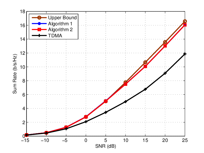
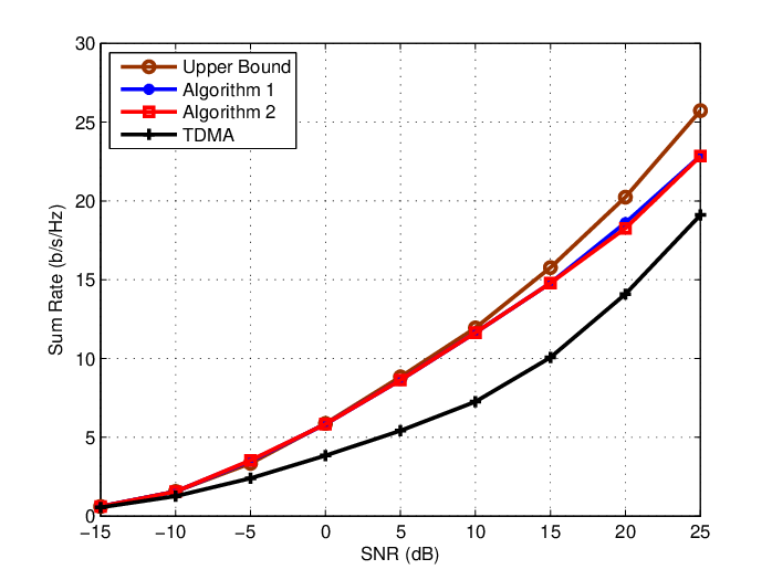
Figure 1 and Figure 2 plot the sum-rate performance of Example 1 and Example 2 achieved by different transmit designs respectively. For Algorithm 2, we compute the exact LAWSR in (15) with the obtained 𝐅~l{\widetilde{{\bf{F}}}}_{l} and 𝚺l{\bf{{\Sigma}}}_{l}. Then, we plot the exact LAWSR. For comparison purpose, we plot the sum rate performances achieved by the “TDMA” case. Also, to evaluate our proposed design, we propose a no-interference upper bound of the MIMO BC with statistical CSI as follows [25]:

R¯upper=∑l=1LμlE[log2det(𝐈Nr+(N0𝐈Nr+𝐇l∑k=l+1L𝚺k𝐇lH)−1𝐇l𝚺l𝐇lH)].\begin{array}[]{l}\overline{R}_{{\rm{upper}}}=\sum\limits_{l=1}^{L}\mu_{l}{E\left[{\log_{2}\det\left({{\bf{I}}_{N_{r}}}\right.}\right.}\\ \hskip 28.45274pt{\left.{\left.{+\left({N_{0}{\bf{I}}_{N_{r}}+{\bf{H}}_{l}\sum\limits_{k=l+1}^{L}{{\bf{\Sigma}}_{k}}}{{{\bf{H}}_{l}^{H}}}\right)^{-1}{\bf{H}}_{l}{\bf{\Sigma}}_{l}{\bf{H}}_{l}^{H}}\right)}\right]}.\end{array} (48)

The upper bound R¯upper\overline{R}_{{\rm{upper}}} is denoted as “Upper Bound” in the figures. It is noted that for the MIMO BC with statistical CSI, the upper bound R¯upper\overline{R}_{{\rm{upper}}} coincides with the WSR of the no-interference channel, which is clearly the best we can expect. Nevertheless, whether this bound is achievable is still unknown.

From Figure 1 and Figure 2, we can make several observations.

  • 1)

    The transmit designs in Algorithm 1 and Algorithm 2 have better sum-rate performance than other design methods throughout the entire SNR region.

  • 2)

    The curves for maximizing the upper bound via Algorithm 2 and maximizing the exact LAWSR directly via Algorithm 1 are virtually the same, but the complexity is different. The method for maximizing the exact LAWSR requires, at each iteration, numerically averaging certain random matrices involving the inverse of instantaneous realizations of the MIMO channels. Thus, the computing effort of Algorithm 2, which does not require such numerical averaging, is significantly less than that of Algorithm 1.

  • 3)

    The proposed designs offer appreciable gains in sum-rate performance when compared against the “TDMA” design. Specifically, at the sum-rate 1010 b/s/Hz, the SNR gains of the proposed precoding designs over the “TDMA” design are approximately 4.54.5 dB and 77 dB for Example 1 and Example 2 respectively.

  • 4)

    The proposed designs perform close to the upper bound R¯upper\overline{R}_{{\rm{upper}}} and approach the bound as the transmit correlation increases.

The matrices 𝐅l\mathbf{F}_{l} and 𝐏l\mathbf{P}_{l} obtained by Algorithm 1 and Algorithm 2 at SNR=0\rm{SNR}=0 dB are given by

1) Example 1:

  • •

    Algorithm 1

    𝐅1\displaystyle\mathbf{F}_{1} =0\displaystyle=0 (49)
    𝐅2\displaystyle\mathbf{F}_{2} =[  0.3240+0.0018​j−0.3206−0.0463​j−0.3200+0.0462​j  0.3232−0.0018​j]\displaystyle=\left[{\begin{array}[]{*{20}c}\ \,0.3240+0.0018j&-0.3206-0.0463j\\ -0.3200+0.0462j&\ \ \,0.3232-0.0018j\\ \end{array}}\right]
    𝐏1\displaystyle{\bf{P}}_{1} =[−0.2712+0.3459​j0.2300−0.0272​j−0.2215+0.3845​j0.2242−0.0590​j]\displaystyle=\left[{\begin{array}[]{*{20}c}-0.2712+0.3459j&0.2300-0.0272j\\ -0.2215+0.3845j&0.2242-0.0590j\\ \end{array}}\right]
    𝐏2\displaystyle{\bf{P}}_{2} =[  0.3406−0.2130​j−0.1300−0.2710​j−0.3051+0.2603​j  0.1687+0.2480​j]\displaystyle=\left[{\begin{array}[]{*{20}c}\ \,0.3406-0.2130j&-0.1300-0.2710j\\ -0.3051+0.2603j&\ \ \,0.1687+0.2480j\\ \end{array}}\right]
  • •

    Algorithm 2

    𝐅1\displaystyle\mathbf{F}_{1} =0\displaystyle=0 (56)
    𝐅2\displaystyle\mathbf{F}_{2} =[  0.3240+0.0018​j−0.3206−0.0463​j−0.3200+0.0462​j  0.3232−0.0018​j]\displaystyle=\left[{\begin{array}[]{*{20}c}\ \,0.3240+0.0018j&-0.3206-0.0463j\\ -0.3200+0.0462j&\ \ \,0.3232-0.0018j\\ \end{array}}\right]
    𝐏1\displaystyle{\bf{P}}_{1} =[−0.2657+0.3435​j0.2280−0.0289​j−0.2244+0.3838​j0.2241−0.0570​j]\displaystyle=\left[{\begin{array}[]{*{20}c}-0.2657+0.3435j&0.2280-0.0289j\\ -0.2244+0.3838j&0.2241-0.0570j\\ \end{array}}\right]
    𝐏2\displaystyle{\bf{P}}_{2} =[  0.3422−0.2143​j−0.1301−0.2727​j−0.3067+0.2613​j  0.1699+0.2488​j]\displaystyle=\left[{\begin{array}[]{*{20}c}\ \,0.3422-0.2143j&-0.1301-0.2727j\\ -0.3067+0.2613j&\ \ \,0.1699+0.2488j\\ \end{array}}\right]

2) Example 2:

  • •

    Algorithm 1

    𝐅1\displaystyle\mathbf{F}_{1} =0\displaystyle=0 (63)
    𝐅2\displaystyle\mathbf{F}_{2} =[  0.1779+0.0023​j−0.1879+0.0347​j−0.3916−0.0373​j  0.3853+0.0162​j]\displaystyle=\left[{\begin{array}[]{*{20}c}\ \,0.1779+0.0023j&-0.1879+0.0347j\\ -0.3916-0.0373j&\ \ \,0.3853+0.0162j\\ \end{array}}\right]
    𝐏1\displaystyle{\bf{P}}_{1} =[−0.2712+0.3459​j0.2300−0.0272​j−0.2215+0.3845​j0.2242−0.0590​j]\displaystyle=\left[{\begin{array}[]{*{20}c}-0.2712+0.3459j&0.2300-0.0272j\\ -0.2215+0.3845j&0.2242-0.0590j\\ \end{array}}\right]
    𝐏2\displaystyle{\bf{P}}_{2} =[  0.3406−0.2130​j−0.1300−0.2710​j−0.3051+0.2603​j  0.1687+0.2480​j]\displaystyle=\left[{\begin{array}[]{*{20}c}\ \,0.3406-0.2130j&-0.1300-0.2710j\\ -0.3051+0.2603j&\ \ \,0.1687+0.2480j\\ \end{array}}\right]
  • •

    Algorithm 2

    𝐅1\displaystyle\mathbf{F}_{1} =0\displaystyle=0 (70)
    𝐅2\displaystyle\mathbf{F}_{2} =[  0.3240+0.0018​j−0.3206−0.0463​j−0.3200+0.0462​j  0.3232−0.0018​j]\displaystyle=\left[{\begin{array}[]{*{20}c}\ \,0.3240+0.0018j&-0.3206-0.0463j\\ -0.3200+0.0462j&\ \ \,0.3232-0.0018j\\ \end{array}}\right]
    𝐏1\displaystyle{\bf{P}}_{1} =[−0.2657+0.3435​j0.2280−0.0289​j−0.2244+0.3838​j0.2241−0.0570​j]\displaystyle=\left[{\begin{array}[]{*{20}c}-0.2657+0.3435j&0.2280-0.0289j\\ -0.2244+0.3838j&0.2241-0.0570j\\ \end{array}}\right]
    𝐏2\displaystyle{\bf{P}}_{2} =[  0.3422−0.2143​j−0.1301−0.2727​j−0.3067+0.2613​j  0.1699+0.2488​j]\displaystyle=\left[{\begin{array}[]{*{20}c}\ \,0.3422-0.2143j&-0.1301-0.2727j\\ -0.3067+0.2613j&\ \ \,0.1699+0.2488j\\ \end{array}}\right]

It should be noted that 𝐅l\mathbf{F}_{l} and 𝐏l\mathbf{P}_{l} obtained by Algorithm 1 and Algorithm 2 maximize the exact LAWSR RsumwR_{\rm sum}^{\rm w} and the upper bound R~upp,sumw\widetilde{R}_{\rm upp,\,sum}^{w}, respectively. Although R~upp,sumw\widetilde{R}_{\rm upp,\,sum}^{w} is close to R~upp,sumw\widetilde{R}_{\rm upp,\,sum}^{w} due to the canceling effect of the bounding error, they are not the same. As a result, the matrices 𝐅l\mathbf{F}_{l} and 𝐏l\mathbf{P}_{l} obtained by Algorithm 1 and Algorithm 2 are close, but not always the same.
Refer to caption
Fig. 1: Sum rates in the fading MIMO BC for different transmit designs and Example 1.
Refer to caption
Fig. 2: Sum rates in the fading MIMO BC for different transmit designs and Example 2.

To further validate the proposed designs, we provide Example 3 and Example 4 as follows. We assume the receiver correlation matrices in both examples are given in (77), (78) at the top of the next page. Transmit correlation matrices of the two examples are given in (79), (80) and (81), (82) at the top of the next page.

𝐑r, 1=[1−0.12−0.18​j 0.08+0.05​j−0.02−0.13​j−0.12+0.18​j1−0.17−0.16​j 0.11+0.04​j 0.08−0.05​j−0.17+0.16​j1−0.17−0.16​j−0.02+0.13​j 0.11−0.04​j−0.17+0.16​j1],{\bf{R}}_{r,\,1}=\left[{\begin{array}[]{*{20}c}1&{-0.12-0.18j}&\ \ {0.08+0.05j}&{-0.02-0.13j}\\ {-0.12+0.18j}&{1}&{-0.17-0.16j}&\ \ {0.11+0.04j}\\ \ \ {0.08-0.05j}&{-0.17+0.16j}&{1}&{-0.17-0.16j}\\ {-0.02+0.13j}&\ \ {0.11-0.04j}&{-0.17+0.16j}&{1}\\ \end{array}}\right], (77)
𝐑r, 2=[1−0.11+0.15​j 0.07+0.04​j−0.01−0.10​j−0.11−0.15​j1 0.10+0.10​j 0.05−0.02​j 0.07−0.04​j 0.10−0.10​j1−0.10−0.20​j−0.01+0.10​j 0.05+0.02​j−0.10+0.20​j1].{\bf{R}}_{r,\,2}=\left[{\begin{array}[]{*{20}c}1&-0.11+0.15j&\ \ 0.07+0.04j&-0.01-0.10j\\ -0.11-0.15j&1&\ \ 0.10+0.10j&\ \ 0.05-0.02j\\ \ \ 0.07-0.04j&\ \ 0.10-0.10j&1&-0.10-0.20j\\ -0.01+0.10j&\ \ 0.05+0.02j&-0.10+0.20j&1\\ \end{array}}\right]. (78)


𝐑t, 1=[10.61+0.34​j0.280.61−0.34​j0.61−0.34​j10.61+0.34​j0.280.280.61−0.34​j10.61+0.34​j0.61+0.34​j0.280.61−0.34​j1],{\bf{R}}_{t,\,1}=\left[{\begin{array}[]{*{20}c}1&0.61+0.34j&0.28&0.61-0.34j\\ 0.61-0.34j&1&0.61+0.34j&0.28\\ 0.28&0.61-0.34j&1&0.61+0.34j\\ 0.61+0.34j&0.28&0.61-0.34j&1\\ \end{array}}\right], (79)
𝐑t, 2=[1−0.24−0.71​j−0.48−0.24+0.71​j−0.24+0.71​j1−0.24−0.71​j−0.48−0.48−0.24+0.71​j1−0.24−0.71​j−0.24−0.71​j−0.48−0.24+0.71​j1].{\bf{R}}_{t,\,2}=\left[{\begin{array}[]{*{20}c}1&-0.24-0.71j&-0.48&-0.24+0.71j\\ -0.24+0.71j&1&-0.24-0.71j&-0.48\\ -0.48&-0.24+0.71j&1&-0.24-0.71j\\ -0.24-0.71j&-0.48&-0.24+0.71j&1\\ \end{array}}\right]. (80)


𝐑t, 1=[10.94+0.01​j0.930.94−0.01​j0.94−0.01​j10.94+0.01​j0.930.930.94−0.01​j10.94+0.01​j0.94+0.01​j0.930.94−0.01​j1],{\bf{R}}_{t,\,1}=\left[{\begin{array}[]{*{20}c}1&{0.94+0.01j}&{0.93}&{0.94-0.01j}\\ {0.94-0.01j}&{1}&{0.94+0.01j}&{0.93}\\ 0.93&0.94-0.01j&1&0.94+0.01j\\ 0.94+0.01j&0.93&0.94-0.01j&1\\ \end{array}}\right], (81)
𝐑t, 2=[10.00−0.92​j−0.920.00+0.92​j0.00+0.92​j10.00−0.92​j−0.92−0.920.00+0.92​j10.00−0.92​j0.00−0.92​j−0.920.00+0.92​j1].{\bf{R}}_{t,\,2}=\left[{\begin{array}[]{*{20}c}1&0.00-0.92j&-0.92&0.00+0.92j\\ 0.00+0.92j&1&0.00-0.92j&-0.92\\ -0.92&0.00+0.92j&1&0.00-0.92j\\ 0.00-0.92j&-0.92&0.00+0.92j&1\\ \end{array}}\right]. (82)


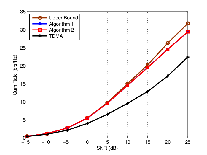
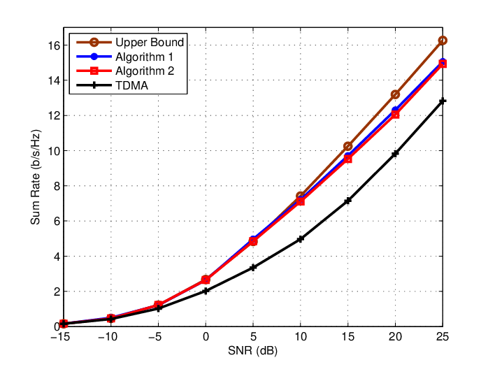
Figure 3 and Figure 4 compare the sum-rate performance given different transmit designs. These results show similar observations as with Example 1 and Example 2. We find that the transmit design based on the upper bound in Proposition 1 performs nearly identically to the design based on the exact result. Moreover, the proposed designs outperform the “TDMA” design throughout the entire SNR region. To achieve a target sum-rate of 1515 b/s/Hz, the SNR gains of the proposed designs over the “TDMA” design are almost 5.25.2 dB and 7.57.5 dB for Example 3 and Example 4 respectively. Also, the performance of the proposed designs is close to the upper bound R¯upper\overline{R}_{{\rm{upper}}}.

Refer to caption
Fig. 3: Sum rates in the fading MIMO BC for different transmit designs and Example 3.
Refer to caption
Fig. 4: Sum rates in the fading MIMO BC for different transmit designs and Example 4.
Refer to caption
Fig. 5: Convergence of Algorithm 1 for Example 2 at different SNR levels.
Refer to caption
Fig. 6: Convergence of Algorithm 1 for Example 4 at different SNR levels.

Figure 5 and Figure 6 illustrate the convergence behavior of Algorithm 1 for different examples at different SNR levels. We can see that in all cases considered, Algorithm 1 converges within a few steps. It should be noted that for some SNR levels, the initialization provided by Algorithm 2 offers the maximal LAWSR. As a result, the sum rate barely increases during the iteration for these SNR levels. The fast convergence behavior of Algorithm 1 implies it can potentially be implemented in practice. However, as indicated above, in each iteration step, Algorithm 1 requires Monte-Carlo procedure. This will increase the implementation complexity. Henceforth, Algorithm 1 can also be utilized to provide a performance limit criterion for other precoding designs in practical systems. To reduce the complexity, we further propose Algorithm 2 which does not need numerical averaging.

In practical scenarios, the channels often include line-of-sight (LOS) paths. To verify the LOS impact on the accuracy of the upper bound, we consider the Rician fading channel model

𝐇l=KK+1𝐇¯𝐥+𝟏𝐊+𝟏𝐑𝐫,𝐥𝟏/𝟐𝐇𝐰𝐑𝐭,𝐥𝟏/𝟐,𝐥=𝟏,𝟐{\bf{H}}_{l}=\sqrt{\frac{K}{{K+1}}}\overline{\bf{H}}_{l}+\sqrt{\frac{1}{{K+1}}}{\bf{R}}_{r,\,l}^{1/2}{\bf{H}}_{w}{\bf{R}}_{t,\,l}^{1/2},\hskip 11.49994ptl=1,2 (83)

where matrix 𝐇l{\bf{H}}_{l} is a deterministic matrix, satisfying tr​(𝐇¯𝐥​𝐇¯𝐥𝐇)=𝐍𝐫​𝐍𝐭\text{tr}(\overline{\bf{H}}_{l}\overline{\bf{H}}_{l}^{H})=N_{r}N_{t}, and K≥0K\geq 0 is the Rician KK-factor. We assume

𝐇¯𝟏=[0.58981.17950.29491.4744],𝐇¯𝟐=[0.38491.15470.38491.5396].\overline{\bf{H}}_{1}={\rm{}}\left[{\begin{array}[]{*{20}c}{{\rm{0}}{\rm{.5898}}}&{{\rm{1}}{\rm{.1795}}}\\ {{\rm{0}}{\rm{.2949}}}&{{\rm{1}}{\rm{.4744}}}\\ \end{array}}\right],\hskip 11.49994pt\overline{\bf{H}}_{2}={\rm{}}\left[{\begin{array}[]{*{20}c}{{\rm{0}}{\rm{.3849}}}&{{\rm{1}}{\rm{.1547}}}\\ {{\rm{0}}{\rm{.3849}}}&{{\rm{1}}{\rm{.5396}}}\\ \end{array}}\right]{\rm{}}. (84)

𝐑r,l\mathbf{R}_{r,\,l} and 𝐑t,l\mathbf{R}_{t,\,l} are chosen as in Example 1. Figure 7 shows the sum rate performance of Algorithm88 8 The main purpose here is to examine the accuracy of the upper bound as the KK-factor increases. Thus, we only simulate Algorithm 2 in Figure 7. 2 in the context of different KK-factors and SNRs. The sum rates achieved by the iterative water-filling algorithm [43] with instantaneous channel matrices, where 𝐇l=𝐇¯𝐥{\bf{H}}_{l}=\overline{\bf{H}}_{l}, l=1,2l=1,2, are also plotted as benchmarks. We observe from Figure 7 that the sum rate performance of Algorithm 2 improves and approaches the sum rates obtained with instantaneous channel matrices as KK increases. This is expected because if the channels of all receivers converge to a constant, (28) indicates that the design based on Theorem 2 tends to be optimal and Algorithm 2 becomes equivalent to the DPC design in [43].

Refer to caption
Fig. 7: Sum rates in the fading MIMO BC for different KK-factors and SNRs via Algorithm 2.

VI Conclusion

This paper has considered the transmit design over the fading MIMO BC with statistical CSI. To address this problem, a linear assignment operation was implemented. We first determined a set of necessary conditions for the optimal transmit design, from which an iterative gradient descent algorithm was developed to maximize the LAWSR but with a high computational complexity. Thus, we employed Jensen’s inequality into two substraction terms of the LAAR for each receiver to average the random component and proved that this results in a strict upper bound of the LAAR. In light of this, a concise closed-form expression of the linear assignment matrix was derived for each receiver in terms of second-order statistics of the CSI. The derived expression captures some well known construction properties of the DPC design in the BC model with instantaneous CSI at the transmitter and has achieved a similar interference mitigation effect as DPC. This immediately permits the application of classical maximum weighted sum-rate algorithms in the MIMO BC model to design the precoding matrices. Then, we formulated a low-complexity transmission scheme via second-order statistics of the CSI based on the obtained precoding matrices and the closed-form linear assignment matrices. Moreover, transmit strategies in two special fading channel models were discussed. Finally, we provided concrete simulation results to illustrate the substantial gains achieved by the proposed designs.

Appendix A Proof of the Theorem 1

We first rewrite 𝚺l=𝐏l​𝐏lH\bm{\Sigma}_{l}=\mathbf{P}_{l}\mathbf{P}_{l}^{H}. Let θ\theta be the Lagrange multiplier associated with the inequality constraint ∑l=1Ltr⁡(𝐏l​𝐏lH)≤P{\sum\nolimits_{l=1}^{L}{{\rm{tr}}\left({{\mathbf{P}}_{l}{\mathbf{P}}_{l}^{H}}\right)\leq P}}. Then, we have the cost function for the optimal design as

L⁡(𝐅,𝐏,λ)=−Rsumw+θ⁡(∑l=1Ltr⁡(𝐏l​𝐏lH)−P).L\left({\bf{F}},{{\bf{P}},\lambda}\right)=-R_{{\rm{sum}}}^{\rm{w}}+\theta\left({\sum\limits_{l=1}^{L}{{\rm{tr}}\left({{\bf{P}}_{l}{\bf{P}}_{l}^{H}}\right)}-P}\right). (85)

By employing similar approaches as those in [50, 51], we define the complex gradient operator as ∇𝐖f=∂f∂𝐖∗\nabla_{{\mathbf{W}}}f=\frac{{\partial f}}{{\partial{\mathbf{W}}^{*}}}. The (i,j)th\left({i,j}\right)^{\rm{th}} element of the matrix 𝐖\mathbf{W} with the complex gradient operator is defined as {∇𝐖f}i,j=∇{𝐖}i,jf=∂f∂{𝐖∗}i,j\left\{{\nabla_{{\mathbf{W}}}f}\right\}_{i,j}=\nabla_{\left\{{\mathbf{W}}\right\}_{i,j}}f=\frac{{\partial f}}{{\partial\left\{{{\mathbf{W}}^{*}}\right\}_{i,j}}}. To this end, the KKT conditions satisfied by the optimal 𝐅l\mathbf{F}_{l}, 𝐏l\mathbf{P}_{l}, l=1,2,⋯,Ll=1,2,\cdots,L, and θ\theta can be expressed as [29, Eq. (5.49)]

∇𝐅lL(𝐅,𝐏,θ)=0,l=1,2,⋯,L\nabla_{{\bf{F}}_{l}}L\left({{\bf{F}},{\bf{P}},\theta}\right)=0,\quad l=1,2,\cdots,L (86)
∇𝐏tL(𝐅,𝐏,θ)=0,t=1,2,⋯,L\nabla_{{\bf{P}}_{t}}L\left({{\bf{F}},{\bf{P}},\theta}\right)=0,\quad t=1,2,\cdots,L (87)
θ⁡(∑l=1Ltr⁡(𝐏l​𝐏lH)−P)=0\theta\left({\sum\limits_{l=1}^{L}{\rm{tr}}\left({{\bf{P}}_{l}{\bf{P}}_{l}^{H}}\right)-P}\right)=0 (88)
∑l=1Ltr⁡(𝐏l​𝐏lH)−P≤0{\sum\limits_{l=1}^{L}{\rm{tr}}\left({{\bf{P}}_{l}{\bf{P}}_{l}^{H}}\right)-P}\leq 0 (89)
θ≥0.\theta\geq 0. (90)

Next, we consider the calculation of ∇𝐅lL​(𝐅,𝐏,θ)\nabla_{{\bf{F}}_{l}}L\left({{\bf{F}},{\bf{P}},\theta}\right). We first express the (m,n)th(m,n)^{\rm{th}} element of the matrix 𝐂l\mathbf{C}_{l} as

{𝐂l}m,n=𝐞mH​(𝐅l​𝚺S,l​𝐅lH+𝚺l)​𝐞n=tr⁡((𝐅l​𝚺S,l​𝐅lH+𝚺l)​𝐞n​𝐞mH)=tr⁡(𝐅l​𝚺S,l​𝐅lH​𝐞n​𝐞mH)+tr⁡(𝚺l​𝐞n​𝐞mH)\begin{array}[]{lll}\left\{{{\bf{C}}_{l}}\right\}_{m,\,n}&{=}&{\bf{e}}_{m}^{H}\left({{\bf{F}}_{l}{\bf{\Sigma}}_{S,\,l}{\bf{F}}_{l}^{H}+{\bf{\Sigma}}_{l}}\right){\bf{e}}_{n}\\ &{=}&{\rm{tr}}\left({\left({{\bf{F}}_{l}{\bf{\Sigma}}_{S,\,l}{\bf{F}}_{l}^{H}+{\bf{\Sigma}}_{l}}\right){\bf{e}}_{n}{\bf{e}}_{m}^{H}}\right)\\ &{=}&{\rm{tr}}\left({{{\bf{F}}_{l}{\bf{\Sigma}}_{S,\,l}{\bf{F}}_{l}^{H}}{\bf{e}}_{n}{\bf{e}}_{m}^{H}}\right)+{\rm{tr}}\left({\bf{\Sigma}}_{l}{\bf{e}}_{n}{\bf{e}}_{m}^{H}\right)\end{array} (91)

where 𝐞m{\bf{e}}_{m} is a unit-vector with one at the mthm^{\rm{th}} element and zeros elsewhere. According to the complex matrix differentiation results [52, Table 4.3], we have

∂{𝐂l}m,n∂𝐅l∗=∂tr⁡(𝐅l​𝚺S,l​𝐅lH​𝐞n​𝐞mH)∂𝐅l∗=𝐞n​𝐞mH​𝐅l​𝚺S,l\displaystyle\frac{{\partial\left\{{{\bf{C}}_{l}}\right\}_{m,\,n}}}{{\partial{\bf{F}}_{l}^{*}}}=\frac{{\partial{\rm{tr}}\left({{{\bf{F}}_{l}{\bf{\Sigma}}_{S,\,l}{\bf{F}}_{l}^{H}}{\bf{e}}_{n}{\bf{e}}_{m}^{H}}\right)}}{{\partial{\bf{F}}_{l}^{*}}}={\bf{e}}_{n}{\bf{e}}_{m}^{H}{\bf{F}}_{l}{\bf{\Sigma}}_{S,\,l} (92)
∂{𝐂l}m,n∂{𝐅l∗}i,j=𝐞iH​𝐞n​𝐞mH​𝐅l​𝚺S,l​𝐞j=𝐞mH​𝐅l​𝚺S,l​𝐞j​𝐞iH​𝐞n\displaystyle\frac{{\partial\left\{{{\bf{C}}_{l}}\right\}_{m,\,n}}}{{\partial\left\{{{\bf{F}}_{l}^{*}}\right\}_{i,\,j}}}={\bf{e}}_{i}^{H}{\bf{e}}_{n}{\bf{e}}_{m}^{H}{\bf{F}}_{l}{\bf{\Sigma}}_{S,\,l}{\bf{e}}_{j}={\bf{e}}_{m}^{H}{\bf{F}}_{l}{\bf{\Sigma}}_{S,\,l}{\bf{e}}_{j}{\bf{e}}_{i}^{H}{\bf{e}}_{n} (93)
∂𝐂l∂{𝐅l∗}i,j=𝐅l​𝚺S,l​𝐞j​𝐞iH.\displaystyle\frac{{\partial{{\bf{C}}_{l}}}}{{\partial\left\{{{\bf{F}}_{l}^{*}}\right\}_{i,\,j}}}={\bf{F}}_{l}{\bf{\Sigma}}_{S,\,l}{\bf{e}}_{j}{\bf{e}}_{i}^{H}. (94)

Following similar steps as those in (92)–(94), we can obtain

∂(𝐓l​(𝐇l)​𝐀lH)∂{𝐅l∗}i,j=𝐓l​(𝐇l)​𝚺S,l​𝐞j​𝐞iH.\frac{{\partial\left({{\bf{T}}_{l}\left({{\bf{H}}_{l}}\right){\bf{A}}_{l}^{H}}\right)}}{{\partial\left\{{{\bf{F}}_{l}^{*}}\right\}_{i,\,j}}}={\bf{T}}_{l}\left({{\bf{H}}_{l}}\right){\bf{\Sigma}}_{S,\,l}{\bf{e}}_{j}{\bf{e}}_{i}^{H}. (95)

Based on the expression for the LAAR in (11), we know that 𝐅l\mathbf{F}_{l} has no relation to RkR_{k} for l≠kl\neq k. As a result, recalling the expression for L⁡(𝐅,𝐏,θ)L\left({{\bf{F}},{\bf{P}},\theta}\right) in (85) and the definition Rsumw=∑l=1Lμl​RlR_{{\rm{sum}}}^{\rm{w}}=\sum\nolimits_{l=1}^{L}\mu_{l}R_{l}, we have ∇𝐅lL​(𝐅,𝐏,θ)=μl​∇𝐅lRl\nabla_{{\bf{F}}_{l}}L\left({{\bf{F}},{\bf{P}},\theta}\right)=\mu_{l}\nabla_{{\bf{F}}_{l}}R_{l}. By exploiting the expression for RlR_{l} in (11) and the matrix derivative rule [53, Eq. (38)], it yields (96) and (97) at the top of the next page.

{∇𝐅lRl}i,j\displaystyle\left\{{\nabla_{{\bf{F}}_{l}}R_{l}}\right\}_{i,\,j} =−log2eE𝐇l[tr(𝚺𝐮l|𝐲l,𝐇l(𝐇l)−1(∂𝐂l∂{𝐅l∗}i,j−∂(𝐓l​(𝐇l)​𝐀lH)∂{𝐅l∗}i,j))]\displaystyle=-\log_{2}e\,E_{\mathbf{H}_{l}}\left[{\rm{tr}}\left({\bm{\Sigma}_{{\bf{u}}_{l}\left|{{\bf{y}}_{l},\,{\bf{H}}_{l}}\right.}\left({{\bf{H}}_{l}}\right)^{-1}}\left(\frac{{\partial{{\bf{C}}_{l}}}}{{\partial\left\{{{\bf{F}}_{l}^{*}}\right\}_{i,\,j}}}-\frac{{\partial\left({{\bf{T}}_{l}\left({{\bf{H}}_{l}}\right){\bf{A}}_{l}^{H}}\right)}}{{\partial\left\{{{\bf{F}}_{l}^{*}}\right\}_{i,\,j}}}\right)\right)\right] (96)
=−log2eE𝐇l[tr(𝚺𝐮l|𝐲l,𝐇l(𝐇l)−1[𝐅l𝚺S,l𝐞j𝐞iH−𝐓l(𝐇l)𝚺S,l𝐞j𝐞iH])].\displaystyle=-\log_{2}e\,E_{\mathbf{H}_{l}}\left[{\rm{tr}}\left({\bm{\Sigma}_{{\bf{u}}_{l}\left|{{\bf{y}}_{l},\,{\bf{H}}_{l}}\right.}\left({{\bf{H}}_{l}}\right)^{-1}\left[{{\bf{F}}_{l}{\bf{\Sigma}}_{S,\,l}{\bf{e}}_{j}{\bf{e}}_{i}^{H}-{\bf{T}}_{l}\left({{\bf{H}}_{l}}\right){\bf{\Sigma}}_{S,\,l}{\bf{e}}_{j}{\bf{e}}_{i}^{H}}\right]}\right)\right]. (97)


Then, we have

∇𝐅lL​(𝐅,𝐏,θ)=μl​∇𝐅lRl=−μllog2eE𝐇l[(𝚺𝐮l|𝐲l,𝐇l(𝐇l)−1(𝐅l−𝐓l(𝐇l))𝚺S,l)].\begin{array}[]{l}\nabla_{{\bf{F}}_{l}}L\left({{\bf{F}},{\bf{P}},\theta}\right)=\mu_{l}\nabla_{{\bf{F}}_{l}}R_{l}=\\ -\mu_{l}\log_{2}eE_{\mathbf{H}_{l}}\left[\left({\bm{\Sigma}_{{\bf{u}}_{l}\left|{{\bf{y}}_{l},\,{\bf{H}}_{l}}\right.}\left({{\bf{H}}_{l}}\right)^{-1}\left({{\bf{F}}_{l}-{\bf{T}}_{l}\left({{\bf{H}}_{l}}\right)}\right){\bf{\Sigma}}_{S,\,l}}\right)\right].\end{array} (98)

Next, we evaluate ∇𝐏tL​(𝐅,𝐏,θ)\nabla_{{\bf{P}}_{t}}L\left({{\bf{F}},{\bf{P}},\theta}\right). By employing the matrix derivative rule in [53, Eq. (33)] and following similar steps as those in (92)–(98), we have

1) t<lt<l

{∇𝐏tRl}i,j=−log2eE[tr(𝚺𝐮l|𝐲l,𝐇l(𝐇l)−1𝐅l𝐏t𝐞j𝐞iH𝐅lH)−tr(𝚺𝐮l|𝐲l,𝐇l(𝐇l)−1𝐅l𝐏t𝐞j𝐞iH𝐓lH(𝐇l))+tr(𝚺𝐮l|𝐲l,𝐇l(𝐇l)−1𝐓lH(𝐇l)𝐇l𝐏t𝐞j𝐞iH𝐓l(𝐇l))]−tr(𝚺𝐮l|𝐲l,𝐇l(𝐇l)−1𝐓l(𝐇l)𝐇l𝐏t𝐞j𝐞iH𝐅lH)\begin{array}[]{l}\left\{\!{\nabla_{{\bf{P}}_{t}}R_{l}}\!\right\}_{i,\,j}\!\!=\!\!-\log_{2}e\,E\left[\!\text{tr}\left(\!{\bm{\Sigma}_{{\bf{u}}_{l}\left|{{\bf{y}}_{l},\,{\bf{H}}_{l}}\right.}\!\left({{\bf{H}}_{l}}\right)^{-1}\!{\bf{F}}_{l}{\bf{P}}_{t}{\bf{e}}_{j}{\bf{e}}_{i}^{H}{\bf{F}}_{l}^{H}}\!\right)\right.\\ \hskip 42.67912pt-\text{tr}\left({\bm{\Sigma}_{{\bf{u}}_{l}\left|{{\bf{y}}_{l},\,{\bf{H}}_{l}}\right.}\left({{\bf{H}}_{l}}\right)^{-1}{\bf{F}}_{l}{\bf{P}}_{t}{\bf{e}}_{j}{\bf{e}}_{i}^{H}{\bf{T}}_{l}^{H}\left({{\bf{H}}_{l}}\!\right)}\!\right)\\ \hskip 14.22636pt\left.+\text{tr}\left({\bm{\Sigma}_{{\bf{u}}_{l}\left|{{\bf{y}}_{l},\,{\bf{H}}_{l}}\right.}\left({{\bf{H}}_{l}}\right)^{-1}{\bf{T}}_{l}^{H}\left({{\bf{H}}_{l}}\right){\bf{H}}_{l}{\bf{P}}_{t}{\bf{e}}_{j}{\bf{e}}_{i}^{H}{\bf{T}}_{l}\left({{\bf{H}}_{l}}\right)}\right)\right]\\ \hskip 14.22636pt-\text{tr}\left({\bm{\Sigma}_{{\bf{u}}_{l}\left|{{\bf{y}}_{l},\,{\bf{H}}_{l}}\right.}\left({{\bf{H}}_{l}}\right)^{-1}{\bf{T}}_{l}\left({{\bf{H}}_{l}}\right){\bf{H}}_{l}{\bf{P}}_{t}{\bf{e}}_{j}{\bf{e}}_{i}^{H}{\bf{F}}_{l}^{H}}\right)\end{array} (99)
∇𝐏tRl=−log2eE[𝐅lH𝚺𝐮l|𝐲l,𝐇l(𝐇l)−1𝐅l𝐏t−𝐓lH(𝐇l)𝚺𝐮l|𝐲l,𝐇l(𝐇l)−1𝐅l𝐏t+𝐓lH(𝐇l)𝚺𝐮l|𝐲l,𝐇l(𝐇l)−1×𝐓l(𝐇l)𝐏t−𝐅lH𝚺𝐮l|𝐲l,𝐇l(𝐇l)−1𝐓l(𝐇l)𝐏t].\begin{array}[]{l}\nabla_{{\bf{P}}_{t}}R_{l}=-\log_{2}e\,E\left[{\bf{F}}_{l}^{H}\bm{\Sigma}_{{\bf{u}}_{l}\left|{{\bf{y}}_{l},\,{\bf{H}}_{l}}\right.}\left({{\bf{H}}_{l}}\right)^{-1}{\bf{F}}_{l}{\bf{P}}_{t}\right.\\ \!-\!{\bf{T}}_{l}^{H}\left({{\bf{H}}_{l}}\right)\!\bm{\Sigma}_{{\bf{u}}_{l}\left|{{\bf{y}}_{l},\,{\bf{H}}_{l}}\right.}\!\left({{\bf{H}}_{l}}\right)^{-1}\!{\bf{F}}_{l}\!{\bf{P}}_{t}\!\!+\!\!{\bf{T}}_{l}^{H}\left({{\bf{H}}_{l}}\right)\!\bm{\Sigma}_{{\bf{u}}_{l}\left|{{\bf{y}}_{l},\,{\bf{H}}_{l}}\right.}\!\left({{\bf{H}}_{l}}\right)^{-1}\\ \hskip 28.45274pt\left.\times{\bf{T}}_{l}\left({{\bf{H}}_{l}}\right){\bf{P}}_{t}-{\bf{F}}_{l}^{H}\bm{\Sigma}_{{\bf{u}}_{l}\left|{{\bf{y}}_{l},\,{\bf{H}}_{l}}\right.}\left({{\bf{H}}_{l}}\right)^{-1}{\bf{T}}_{l}\left({{\bf{H}}_{l}}\right){\bf{P}}_{t}\right].\\ \end{array} (100)

2) t=lt=l

{∇𝐏tRl}i,j=log2⁡e​tr​((𝐏tH)−1​𝐞j​𝐞iH)−log2eE[tr(𝚺𝐮l|𝐲l,𝐇l(𝐇l)−1𝐏t𝐞j𝐞iH)−tr(𝚺𝐮l|𝐲l,𝐇l(𝐇l)−1𝐏t𝐞j𝐞iH𝐓lH(𝐇l))+tr(𝚺𝐮l|𝐲l,𝐇l(𝐇l)−1𝐓l(𝐇l)𝐏t𝐞j𝐞iH𝐓lH(𝐇l))−tr(𝚺𝐮l|𝐲l,𝐇l(𝐇l)−1𝐓l(𝐇l)𝐏t𝐞j𝐞iH)]\begin{array}[]{l}\left\{{\nabla_{{\bf{P}}_{t}}R_{l}}\right\}_{i,\,j}=\log_{2}e\,\text{tr}\left({\left({{\bf{P}}_{t}^{H}}\right)^{-1}{\bf{e}}_{j}{\bf{e}}_{i}^{H}}\right)\\ \hskip 28.45274pt-\log_{2}e\,E\left[\text{tr}\left({\bm{\Sigma}_{{\bf{u}}_{l}\left|{{\bf{y}}_{l},\,{\bf{H}}_{l}}\right.}\left({{\bf{H}}_{l}}\right)^{-1}{\bf{P}}_{t}{\bf{e}}_{j}{\bf{e}}_{i}^{H}}\right)\right.\\ \hskip 28.45274pt-\text{tr}\left({\bm{\Sigma}_{{\bf{u}}_{l}\left|{{\bf{y}}_{l},\,{\bf{H}}_{l}}\right.}\left({{\bf{H}}_{l}}\right)^{-1}{\bf{P}}_{t}{\bf{e}}_{j}{\bf{e}}_{i}^{H}{\bf{T}}_{l}^{H}\left({{\bf{H}}_{l}}\right)}\right)\\ \hskip 14.22636pt+\text{tr}\left({\bm{\Sigma}_{{\bf{u}}_{l}\left|{{\bf{y}}_{l},\,{\bf{H}}_{l}}\right.}\left({{\bf{H}}_{l}}\right)^{-1}{\bf{T}}_{l}\left({{\bf{H}}_{l}}\right){\bf{P}}_{t}{\bf{e}}_{j}{\bf{e}}_{i}^{H}{\bf{T}}_{l}^{H}\left({{\bf{H}}_{l}}\right)}\right)\\ \hskip 28.45274pt\left.-\text{tr}\left({\bm{\Sigma}_{{\bf{u}}_{l}\left|{{\bf{y}}_{l},\,{\bf{H}}_{l}}\right.}\left({{\bf{H}}_{l}}\right)^{-1}{\bf{T}}_{l}\left({{\bf{H}}_{l}}\right){\bf{P}}_{t}{\bf{e}}_{j}{\bf{e}}_{i}^{H}}\right)\right]\\ \end{array} (101)
∇𝐏tRl=log2e(𝐏tH)−1−log2eE[𝚺𝐮l|𝐲l,𝐇l(𝐇l)−1𝐏t−𝐓lH(𝐇l)𝚺𝐮l|𝐲l,𝐇l(𝐇l)−1𝐏t+𝐓lH(𝐇l)𝚺𝐮l|𝐲l,𝐇l(𝐇l)−1𝐓l(𝐇l)𝐏t−𝚺𝐮l|𝐲l,𝐇l(𝐇l)−1𝐓l(𝐇l)𝐏t].\begin{array}[]{l}\nabla_{{\bf{P}}_{t}}R_{l}=\log_{2}e\,\left({{\bf{P}}_{t}^{H}}\right)^{-1}-\log_{2}e\,E\left[\bm{\Sigma}_{{\bf{u}}_{l}\left|{{\bf{y}}_{l},\,{\bf{H}}_{l}}\right.}\left({{\bf{H}}_{l}}\right)^{-1}{\bf{P}}_{t}\right.\\ \!-\!{\bf{T}}_{l}^{H}\left({{\bf{H}}_{l}}\right)\bm{\Sigma}_{{\bf{u}}_{l}\left|{{\bf{y}}_{l},\,{\bf{H}}_{l}}\right.}\!\left({{\bf{H}}_{l}}\right)^{-1}{\bf{P}}_{t}\!+\!{\bf{T}}_{l}^{H}\left({{\bf{H}}_{l}}\right)\bm{\Sigma}_{{\bf{u}}_{l}\left|{{\bf{y}}_{l},\,{\bf{H}}_{l}}\right.}\!\left({{\bf{H}}_{l}}\right)^{-1}\\ \hskip 56.9055pt\left.{\bf{T}}_{l}\left({{\bf{H}}_{l}}\right){\bf{P}}_{t}-\bm{\Sigma}_{{\bf{u}}_{l}\left|{{\bf{y}}_{l},\,{\bf{H}}_{l}}\right.}\left({{\bf{H}}_{l}}\right)^{-1}{\bf{T}}_{l}\left({{\bf{H}}_{l}}\right){\bf{P}}_{t}\right].\\ \end{array} (102)

3) t>lt>l

{∇𝐏tRl}i,j=−log2eE[tr(𝚺𝐮l|𝐲l,𝐇l(𝐇l)−1𝐓l(𝐇l)𝐏t×𝐞j𝐞iH𝐓lH(𝐇l))]\begin{array}[]{l}\left\{{\nabla_{{\bf{P}}_{t}}R_{l}}\right\}_{i,\,j}=-\log_{2}e\,E\left[\text{tr}\left({\bm{\Sigma}_{{\bf{u}}_{l}\left|{{\bf{y}}_{l},\,{\bf{H}}_{l}}\right.}\left({{\bf{H}}_{l}}\right)^{-1}{\bf{T}}_{l}\left({{\bf{H}}_{l}}\right){\bf{P}}_{t}}\right.\right.\\ \hskip 142.26378pt\left.\left.{{\times\bf{e}}_{j}{\bf{e}}_{i}^{H}{\bf{T}}_{l}^{H}\left({{\bf{H}}_{l}}\right)}\right)\right]\end{array} (103)
{∇𝐏iRl}=−log2eE[𝐓lH(𝐇l)𝚺𝐮l|𝐲l,𝐇l(𝐇l)−1𝐓l(𝐇l)].\left\{{\nabla_{{\bf{P}}_{i}}R_{l}}\right\}\!=\!-\log_{2}e\,E\left[{\bf{T}}_{l}^{H}\left({{\bf{H}}_{l}}\right)\bm{\Sigma}_{{\bf{u}}_{l}\left|{{\bf{y}}_{l},\,{\bf{H}}_{l}}\right.}\!\left({{\bf{H}}_{l}}\right)^{-1}{\bf{T}}_{l}\left({{\bf{H}}_{l}}\right)\right]. (104)

Based on (15) and ∇𝐏t(∑l=1L𝐏l​𝐏lH)=𝐏t\nabla_{{\bf{P}}_{t}}\left({\sum\nolimits_{l=1}^{L}{{\bf{P}}_{l}{\bf{P}}_{l}^{H}}}\right)={\bf{P}}_{t}, ∇𝐏tL​(𝐅,𝐏,θ)\nabla_{{\bf{P}}_{t}}L\left({{\bf{F}},{\bf{P}},\theta}\right) can be expressed as

∇𝐏tL​(𝐅,𝐏,θ)=−(∑l=1t−1μl​∇𝐏tRl+μt​∇𝐏tRtCLOSE+∑l=t+1Lμl∇𝐏tRl)+θ𝐏t.\begin{array}[]{l}\nabla_{{\bf{P}}_{t}}L\left({{\bf{F}},{\bf{P}},\theta}\right)\!=\!-\left({\sum\limits_{l=1}^{t-1}\mu_{l}{\nabla_{{\bf{P}}_{t}}R_{l}}+\mu_{t}\nabla_{{\bf{P}}_{t}}R_{t}}\right.\\ \hskip 56.9055pt\left.{+\sum\limits_{l=t+1}^{L}{\mu_{l}\nabla_{{\bf{P}}_{t}}R_{l}}}\right)+\theta{\bf{P}}_{t}.\end{array} (105)

Finally, the theorem can be proved by combining (86)–(90), (98), (100), (102), (104), and (105), along with some simplifications.

Appendix B Proof of the Theorem 2

Before we present the proof, we find the following two lemmas useful.

Lemma 1

Assume 𝐗≻𝟎\mathbf{X}\succ\mathbf{0} is a N×NN\times N random matrix with E⁡[𝐗]=𝐌xE[\mathbf{X}]=\mathbf{M}_{x}. Then, the following result holds

E⁡[𝐗−1]⪰𝐌x−1.E\left[{{\bf{X}}^{-1}}\right]\succeq\mathbf{M}_{x}^{-1}. (106)
Proof:

Let ℋN​(J)\mathcal{H}^{N}(J) denote the space of all Hermitian N×NN\times N matrices whose eigenvalues all fall within JJ. Then, we define a matrix function f:J↦Jf:J\mapsto J, given by

f⁡(𝐓)=𝐓−1.f\left({\bf{T}}\right)={\bf{T}}^{-1}. (107)

According to [54, Lemma 2.5], we know that ff is a strictly matrix convex function. Let 𝐓=𝐓1+a⁡(𝐓2−𝐓1)=(1−a)​𝐓1+a​𝐓2\mathbf{T}=\mathbf{T}_{1}+a(\mathbf{T}_{2}-\mathbf{T}_{1})=(1-a)\mathbf{T}_{1}+a\mathbf{T}_{2}, 0≤a≤10\leq a\leq 1. Then, recalling the definition of matrix convex function in [54, Definition 2.2], it yields

(1−a)​f​(𝐓1)+a​f​(𝐓2)⪰f⁡(𝐓).(1-a)f(\mathbf{T}_{1})+af(\mathbf{T}_{2})\succeq f({\bf{T}}). (108)

Rewriting (108), we have

f⁡(𝐓2)−f⁡(𝐓)⪰1−aa​(f⁡(𝐓)−f⁡(𝐓1)).f\left({{\bf{T}}_{2}}\right)-f\left({\bf{T}}\right)\succeq\frac{{1-a}}{a}\left({f\left({\bf{T}}\right)-f\left({{\bf{T}}_{1}}\right)}\right). (109)

Considering the Taylor expansion of the matrix function in [54, Definition 3.1], f⁡(𝐓)−f⁡(𝐓1){f\left({\bf{T}}\right)-f\left({{\bf{T}}_{1}}\right)} can be expressed as

f⁡(𝐓)−f⁡(𝐓1)=f(1)​(𝐓1)​[𝐓−𝐓1]+o⁡(‖𝐓−𝐓1‖F)​𝐈N=a​f(1)​(𝐓1)​[𝐓2−𝐓1]+o⁡(a​‖(𝐓2−𝐓1)‖F)​𝐈N\begin{array}[]{l}f\left({\bf{T}}\right)-f\left({{\bf{T}}_{1}}\right)\\ =f^{\left(1\right)}\left({{\bf{T}}_{1}}\right)[{\bf{T}}-{\bf{T}}_{1}]+o\left({\left\|{{\bf{T}}-{\bf{T}}_{1}}\right\|_{F}}\right){\bf{I}}_{N}\\ =af^{\left(1\right)}\left({{\bf{T}}_{1}}\right)[{\bf{T}}_{2}-{\bf{T}}_{1}]+o\left({a\left\|{\left({{\bf{T}}_{2}-{\bf{T}}_{1}}\right)}\right\|_{F}}\right){\bf{I}}_{N}\end{array} (110)

where f(1)​(𝐓1)f^{\left(1\right)}\left({{\bf{T}}_{1}}\right) is a Hermitian symmetric multi-linear mapping on the space ℋN\mathcal{H}^{N}. Plugging (110) into (109) and taking the limit as a→0a\rightarrow 0, the right term of (109) becomes

lima→01−aa​(f⁡(𝐓)−f⁡(𝐓1))=f(1)​(𝐓1)​[𝐓2−𝐓1]+lima→0(1−a)a​o​(a​‖(𝐓2−𝐓1)‖F)​𝐈N=f(1)​(𝐓1)​[𝐓2−𝐓1].\begin{array}[]{l}\mathop{\lim}\limits_{a\to 0}\frac{{1-a}}{a}\left({f\left({\bf{T}}\right)-f\left({{\bf{T}}_{1}}\right)}\right)\\ =f^{\left(1\right)}\left({{\bf{T}}_{1}}\right)\left[{{\bf{T}}_{2}-{\bf{T}}_{1}}\right]+\mathop{\lim}\limits_{a\to 0}\frac{{\left({1-a}\right)}}{a}o\left({a\left\|{\left({{\bf{T}}_{2}-{\bf{T}}_{1}}\right)}\right\|_{F}}\right){\bf{I}}_{N}\\ =f^{\left(1\right)}\left({{\bf{T}}_{1}}\right)\left[{{\bf{T}}_{2}-{\bf{T}}_{1}}\right].\end{array} (111)

Synchronously, when a→0a\rightarrow 0, the left term of (109) can be written as

lima→0f⁡(𝐓2)−f⁡(𝐓)=f⁡(𝐓2)−f⁡(𝐓1).\mathop{\lim}\limits_{a\to 0}f\left({{\bf{T}}_{2}}\right)-f\left({\bf{T}}\right)=f\left({{\bf{T}}_{2}}\right)-f\left({{\bf{T}}_{1}}\right). (112)

Eqs. (111) and (112) imply the following result for arbitrary N×NN\times N Hermitian matrices 𝐓1{\bf{T}}_{1} and 𝐓2{\bf{T}}_{2}

f⁡(𝐓2)−f⁡(𝐓1)⪰f(1)​(𝐓1)​[𝐓2−𝐓1].f\left({{\bf{T}}_{2}}\right)-f\left({{\bf{T}}_{1}}\right)\succeq f^{\left(1\right)}\left({{\bf{T}}_{1}}\right)\left[{{\bf{T}}_{2}-{\bf{T}}_{1}}\right]. (113)

By setting 𝐓1=𝐌x\mathbf{T}_{1}=\mathbf{M}_{x}, 𝐓2=𝐗\mathbf{T}_{2}=\mathbf{X}, and evaluating the expectations of both sides of (113), it yields

E⁡[f⁡(𝐗)]−f⁡(𝐌x)⪰f(1)​(𝐌x)​[E⁡[𝐗]−𝐌x]=0E\left[f\left({{\bf{X}}}\right)\right]-f\left(\mathbf{M}_{x}\right)\succeq f^{\left(1\right)}\left({\mathbf{M}_{x}}\right)\left[E\left[{\bf{X}}\right]-\mathbf{M}_{x}\right]=0 (114)

which completes the proof of the lemma. ∎

Lemma 2

Assume 𝐘⪰𝟎\mathbf{Y}\succeq\mathbf{0} is a N×NN\times N random matrix with E⁡[𝐘]=𝐌yE[\mathbf{Y}]=\mathbf{M}_{y}. 𝐀\mathbf{A} and 𝐁\mathbf{B} are N×NN\times N constant matrices satisfying 𝐀≻𝟎\mathbf{A}\succ\mathbf{0}, 𝐁≻𝟎\mathbf{B}\succ\mathbf{0}, and 𝐀−𝐁⪰𝟎\mathbf{A}-\mathbf{B}\succeq\mathbf{0}. Then, the following inequality holds

E⁡[log⁡det2⁡(𝐘𝐀+𝐈N)]−E⁡[log⁡det2⁡(𝐘𝐁+𝐈N)]≤log⁡det2⁡(𝐌y​𝐀+𝐈N)−log⁡det2⁡(𝐌y​𝐁+𝐈N).\begin{array}[]{l}E\left[{\log_{2}\det\left({{\bf{YA}}+{\bf{I}}_{N}}\right)}\right]-E\left[{\log_{2}\det\left({{\bf{YB}}+{\bf{I}}_{N}}\right)}\right]\leq\\ \hskip 28.45274pt\log_{2}\det\left({\mathbf{M}_{y}{\bf{A}}+{\bf{I}}_{N}}\right)-\log_{2}\det\left({\mathbf{M}_{y}{\bf{B}}+{\bf{I}}_{N}}\right).\end{array} (115)
Proof:

We define the function g⁡(𝐓)g(\mathbf{T}) as follows

g⁡(𝐓)=log⁡det2⁡(𝐌y​𝐓+𝐈N)−E⁡[log⁡det2⁡(𝐘𝐓+𝐈N)].g(\mathbf{T})=\log_{2}\det\left(\mathbf{M}_{y}\mathbf{T}+\mathbf{I}_{N}\right)-{{E}}\left[\log_{2}\det(\mathbf{YT}+\mathbf{I}_{N})\right]. (116)

Also, we construct a composite function h⁡(ω)h(\omega) as

h⁡(ω):=g⁡[(1−ω)​𝐁+ω​𝐀]=g⁡(𝐔),0≤ω≤1.h\left(\omega\right):=g\left[{\left({1-\omega}\right){\bf{B}}+\omega{\bf{A}}}\right]=g\left(\mathbf{U}\right),\quad 0\leq\omega\leq 1. (117)

Since 𝐀≻𝟎\mathbf{A}\succ\mathbf{0} and 𝐁≻𝟎\mathbf{B}\succ\mathbf{0}, it can be readily identified that 𝐔≻𝟎\mathbf{U}\succ\mathbf{0}. Moreover, from (117), we have

h⁡(0)=g⁡(𝐁),h⁡(1)=g⁡(𝐀).h\left(0\right)=g\left({\bf{B}}\right),\quad h\left(1\right)=g\left({\bf{A}}\right). (118)

Results in (118) suggest to consider

g⁡(𝐀)−g⁡(𝐁)=h⁡(1)−h⁡(0)=∫01d​h​(ω)d​ω​𝑑ω.g\left({\bf{A}}\right)-g\left({\bf{B}}\right)=h\left(1\right)-h\left(0\right)=\int_{0}^{1}{\frac{{dh\left(\omega\right)}}{{d\omega}}}d\omega. (119)

Application of the chain rule of the derivative leads to

d​h​(ω)d​ω\displaystyle\frac{{dh\left(\omega\right)}}{{d\omega}} =∑r=1N∑s=1N{∂g⁡(𝐔)∂𝐔}r,s×{dd​ω​(ω​𝐀+(1−ω)​𝐁)}r,s\displaystyle=\sum\limits_{r=1}^{N}{\sum\limits_{s=1}^{N}{\left\{{\frac{{\partial g\left({\bf{U}}\right)}}{{\partial{\bf{U}}}}}\right\}_{r,s}}}\!\!\times\!\!\left\{{\frac{d}{{d\omega}}\left({\omega{\bf{A}}\!\!+\!\!\left({1-\omega}\right){\bf{B}}}\right)}\right\}_{r,s} (120)
=∑r=1N∑s=1N{∂g⁡(𝐔)∂𝐔}r,s×{𝐀−𝐁}r,s.\displaystyle=\sum\limits_{r=1}^{N}{\sum\limits_{s=1}^{N}{\left\{{\frac{{\partial g\left({\bf{U}}\right)}}{{\partial{\bf{U}}}}}\right\}_{r,s}}}\times\left\{{{\bf{A}}-{\bf{B}}}\right\}_{r,s}. (121)

Following similar approaches as those in (91)–(98) and keeping in mind that 𝐔≻𝟎\mathbf{U}\succ\mathbf{0}, we can obtain

∂g⁡(𝐔)∂𝐔\displaystyle\frac{{\partial g\left({\bf{U}}\right)}}{{\partial{\bf{U}}}} =(𝐌y​𝐔+𝐈N)−1​𝐌y−E⁡[(𝐘𝐔+𝐈N)−1​𝐘]\displaystyle=\left({\mathbf{M}_{y}{\bf{U}}+{\bf{I}}_{N}}\right)^{-1}{\bf{M}}_{y}-E\left[{\left({{\bf{YU}}+{\bf{I}}_{N}}\right)^{-1}}{\bf{Y}}\right] (122)
=(𝐌y​𝐔+𝐈N)−1​[𝐌y​𝐔+𝐈N−𝐈N]​𝐔−1\displaystyle=\left({\mathbf{M}_{y}{\bf{U}}+{\bf{I}}_{N}}\right)^{-1}\left[{\mathbf{M}_{y}{\bf{U}}+{\bf{I}}_{N}-{\bf{I}}_{N}}\right]{\bf{U}}^{-1}
−E⁡[(𝐘𝐔+𝐈N)−1​[𝐘𝐔+𝐈N−𝐈N]​𝐔−1]\displaystyle\hskip 5.69046pt-E\left[\left({\mathbf{Y}{\bf{U}}+{\bf{I}}_{N}}\right)^{-1}\left[{\mathbf{Y}{\bf{U}}+{\bf{I}}_{N}-{\bf{I}}_{N}}\right]{\bf{U}}^{-1}\right] (123)
=𝐔−1−(𝐌y​𝐔+𝐈N)−1​𝐔−1\displaystyle={\bf{U}}^{-1}-\left({\mathbf{M}_{y}{\bf{U}}+{\bf{I}}_{N}}\right)^{-1}{\bf{U}}^{-1}
−𝐔−1+E⁡[(𝐘𝐔+𝐈N)−1​𝐔−1]\displaystyle\hskip 28.45274pt-{\bf{U}}^{-1}+E\left[\left({\mathbf{Y}{\bf{U}}+{\bf{I}}_{N}}\right)^{-1}{\bf{U}}^{-1}\right] (124)
=E⁡[(𝐔𝐘𝐔+𝐔)−1]−(𝐔𝐌y​𝐔+𝐔)−1.\displaystyle=E\left[{\left({{\bf{UYU}}+{\bf{U}}}\right)^{-1}}\right]-\left({{\bf{UM}}_{y}{\bf{U}}+{\bf{U}}}\right)^{-1}. (125)

Applying Lemma 1 to (124), yields

∂g⁡(𝐔)∂𝐔⪰𝟎.\frac{{\partial g\left({\bf{U}}\right)}}{{\partial{\bf{U}}}}\succeq\mathbf{0}. (126)

Recalling 𝐀−𝐁⪰𝟎\mathbf{A}-\mathbf{B}\succeq\mathbf{0}, the result in (126), and the Schur Product Theorem in [55, Theorem 7.5.3], we have

∂g⁡(𝐔)∂𝐔∘(𝐀−𝐁)⪰𝟎\frac{{\partial g\left({\bf{U}}\right)}}{{\partial{\bf{U}}}}\circ(\mathbf{A}-\mathbf{B})\succeq\mathbf{0} (127)

which implies that

∑r=1N∑s=1N{∂g⁡(𝐔)∂𝐔}r,s×{𝐀−𝐁}r,s≥0.\sum\limits_{r=1}^{N}{\sum\limits_{s=1}^{N}{\left\{{\frac{{\partial g\left({\bf{U}}\right)}}{{\partial{\bf{U}}}}}\right\}_{r,s}}}\times\left\{{{\bf{A}}-{\bf{B}}}\right\}_{r,s}\geq 0. (128)

Then, combining (119), (121), and (128), we have

g⁡(𝐀)−g⁡(𝐁)≥0g\left({\bf{A}}\right)-g\left({\bf{B}}\right)\geq 0 (129)

which completes the proof of the lemma. ∎

Now we begin to prove Lemma 2. As mentioned in Section II, when discussing the linear assignment capacity, similar to the assumption in [25], we assume 𝚺l≻𝟎\mathbf{\Sigma}_{l}\succ\mathbf{0}. Henceforth, we know that 𝐂l\mathbf{C}_{l} is invertible. To this end, log2det(𝚺𝐮l|𝐲l,𝐇l(𝐇l)){\log_{2}\det\left({\bf{\Sigma}}_{{\mathbf{u}_{l}}\left|{{\mathbf{y}_{l}},{\mathbf{H}_{l}}}\right.}\left({\mathbf{H}_{l}}\right)\right)} in (11) can be reexpressed as

log2det(𝚺𝐮l|𝐲l,𝐇l(𝐇l))\displaystyle\log_{2}\det\left({{\bf{\Sigma}}_{{\bf{u}}_{l}\left|{{\bf{y}}_{l},{\bf{H}}_{l}}\right.}\left({\bf{H}}_{l}\right)}\right)
=log⁡det2⁡(𝐂l)\displaystyle=\log_{2}\det\left({\bf{C}}_{l}\right)
+log⁡det2⁡(𝐈Nt−𝐂l−1​𝐀l​𝐇lH​[𝐇𝐁l​𝐇lH+𝚺Z,l]−1​𝐇l​𝐀lH)\displaystyle+\log_{2}\det\left({{\bf{I}}_{N_{t}}-{\bf{C}}_{l}^{-1}{\bf{A}}_{l}\mathbf{H}_{l}^{H}\left[{{\bf{H}}\mathbf{B}_{l}\mathbf{H}_{l}^{H}+{\bf{\Sigma}}_{Z,\,l}}\right]^{-1}{\bf{H}}_{l}\mathbf{A}_{l}^{H}}\right) (130)
=(a)log⁡det2⁡(𝐂l)\displaystyle\mathop{=}\limits^{\left(a\right)}\log_{2}\det\left({\bf{C}}_{l}\right)
+log⁡det2⁡(𝐈Nt−𝐇l​𝐀lH​𝐂l−1​𝐀l​𝐇lH​[𝐇𝐁l​𝐇lH+𝚺Z,l]−1)\displaystyle+\log_{2}\det\left({{\bf{I}}_{N_{t}}-{\bf{H}}_{l}\mathbf{A}_{l}^{H}{\bf{C}}_{l}^{-1}{\bf{A}}_{l}\mathbf{H}_{l}^{H}\left[{{\bf{H}}\mathbf{B}_{l}\mathbf{H}_{l}^{H}+{\bf{\Sigma}}_{Z,\,l}}\right]^{-1}}\right) (131)
=log⁡det2⁡(𝐂l)+log⁡det2⁡(𝐇l​(𝐁l−𝐀lH​𝐂l−1​𝐀l)​𝐇lH+𝚺Z,l)\displaystyle=\log_{2}\det\left({\bf{C}}_{l}\right)\!+\!\log_{2}\det\left({{\bf{H}}_{l}\left({{\bf{B}}_{l}\!\!-\!\!{\bf{A}}_{l}^{H}{\bf{C}}_{l}^{-1}{\bf{A}}}_{l}\right){\bf{H}}_{l}^{H}\!\!+\!\!{\bf{\Sigma}}_{Z,\,l}}\right)
−log⁡det2⁡(𝐇l​𝐁l​𝐇lH+𝚺Z,l)\displaystyle\hskip 56.9055pt-\log_{2}{\det\left({{\bf{H}}_{l}\mathbf{B}_{l}\mathbf{H}_{l}^{H}+{\bf{\Sigma}}_{Z,\,l}}\right)} (132)
=log⁡det2⁡(𝐂l)\displaystyle=\log_{2}\det\left({\bf{C}}_{l}\right)
+log⁡det2⁡(𝐇l​(𝐃l+∑t=l+1L𝚺t)​𝐇lH+N0​𝐈Nr)\displaystyle\hskip 5.69046pt+\log_{2}\det\left({{\bf{H}}_{l}\left(\mathbf{D}_{l}+\sum\limits_{t=l+1}^{L}{\mathbf{\Sigma}_{t}}\right)\mathbf{H}_{l}^{H}+N_{0}\mathbf{I}_{N_{r}}}\right)
−log⁡det2⁡(𝐇l​(𝐁l+∑t=l+1L𝚺t)​𝐇lH+N0​𝐈Nr)\displaystyle-\log_{2}\det\left({{\bf{H}}_{l}\left(\mathbf{B}_{l}+\sum\limits_{t=l+1}^{L}{\mathbf{\Sigma}_{t}}\right)\mathbf{H}_{l}^{H}+N_{0}\mathbf{I}_{N_{r}}}\right) (133)
=(b)log⁡det2⁡(𝐂l)\displaystyle\mathop{=}\limits^{\left(b\right)}\log_{2}\det\left({\bf{C}}_{l}\right)
+log⁡det2⁡(𝐇lH​𝐇l​(𝐃l+∑t=l+1L𝚺t)+N0​𝐈Nt)\displaystyle\hskip 5.69046pt+\log_{2}\det\left(\mathbf{H}_{l}^{H}{{\bf{H}}_{l}\left(\mathbf{D}_{l}+\sum\limits_{t=l+1}^{L}{\mathbf{\Sigma}_{t}}\right)+N_{0}\mathbf{I}_{N_{t}}}\right)
+(Nr−Nt)​log2​N0\displaystyle\hskip 56.9055pt+(N_{r}-N_{t})\log_{2}N_{0}
−log⁡det2⁡(𝐇lH​𝐇l​(𝐁l+∑t=l+1L𝚺t)+N0​𝐈Nt)\displaystyle\hskip 5.69046pt-\log_{2}\det\left(\mathbf{H}_{l}^{H}{{\bf{H}}_{l}\left(\mathbf{B}_{l}+\sum\limits_{t=l+1}^{L}{\mathbf{\Sigma}_{t}}\right)+N_{0}\mathbf{I}_{N_{t}}}\right)
−(Nr−Nt)​log2​N0\displaystyle\hskip 56.9055pt-(N_{r}-N_{t})\log_{2}N_{0} (134)

where equalities (a) and (b) are obtained according to the determinant identity det(𝐗+𝐀𝐁)=det(𝐗)​det(𝐈+𝐁𝐗−1​𝐀)\det(\mathbf{X}+\mathbf{AB})=\det(\mathbf{X})\det(\mathbf{I}+\mathbf{BX}^{-1}\mathbf{A}).

Since 𝚺l≻𝟎\mathbf{\Sigma}_{l}\succ\mathbf{0}, it yields 𝐁l≻𝟎\mathbf{B}_{l}\succ\mathbf{0}, ∑t=l+1L𝚺t≻𝟎\sum\nolimits_{t=l+1}^{L}{\mathbf{\Sigma}_{t}}\succ\mathbf{0}, and 𝐁l−𝐃l=𝐀lH​𝐂l​𝐀l⪰𝟎\mathbf{B}_{l}-\mathbf{D}_{l}=\mathbf{A}_{l}^{H}\mathbf{C}_{l}\mathbf{A}_{l}\succeq\mathbf{0}. Next, we need to prove that 𝐃l≻𝟎\mathbf{D}_{l}\succ\mathbf{0}.

Let 𝐮\mathbf{u} and 𝐯\mathbf{v} be two N×1N\times 1 constant non-zero vectors. We begin by considering

[𝐮H𝐯H]​[𝚺S,l𝚺S,l​𝐅lH𝐅l​𝚺S,l𝐅l​𝚺S,l​𝐅lH]​[𝐮𝐯]\displaystyle\left[{{\bf{u}}^{H}\quad{\bf{v}}^{H}}\right]\left[{\begin{array}[]{*{20}c}{{\bf{\Sigma}}_{S,\,l}}&{{\bf{\Sigma}}_{S,\,l}{\bf{F}}_{l}^{H}}\\ {{\bf{F}}_{l}{\bf{\Sigma}}_{S,\,l}}&{{\bf{F}}_{l}{\bf{\Sigma}}_{S,\,l}{\bf{F}}_{l}^{H}}\end{array}}\right]\left[\begin{array}[]{l}{\bf{u}}\\ {\bf{v}}\\ \end{array}\right]
=𝐮H​𝚺S,l​𝐮+𝐮H​𝚺S,l​𝐅lH​𝐯+𝐯H​𝐅l​𝚺S,l​𝐮+𝐯H​𝐅l​𝚺S,l​𝐅lH​𝐯\displaystyle={\bf{u}}^{H}{\bf{\Sigma}}_{S,\,l}{\bf{u}}\!\!+\!\!{\bf{u}}^{H}{\bf{\Sigma}}_{S,\,l}{\bf{F}}_{l}^{H}{\bf{v}}\!\!+\!\!{\bf{v}}^{H}{\bf{F}}_{l}{\bf{\Sigma}}_{S,\,l}{\bf{u}}\!+\!{\bf{v}}^{H}{\bf{F}}_{l}{\bf{\Sigma}}_{S,\,l}{\bf{F}}_{l}^{H}{\bf{v}} (139)
=𝐮H​(𝚺S,l​𝐮+𝚺S,l​𝐅lH​𝐯)+𝐯H​𝐅l​(𝚺S,l​𝐮+𝚺S,l​𝐅lH​𝐯)\displaystyle={\bf{u}}^{H}\left({{\bf{\Sigma}}_{S,\,l}{\bf{u}}+{\bf{\Sigma}}_{S,\,l}{\bf{F}}_{l}^{H}{\bf{v}}}\right)+{\bf{v}}^{H}{\bf{F}}_{l}\left({{\bf{\Sigma}}_{S,\,l}{\bf{u}}+{\bf{\Sigma}}_{S,\,l}{\bf{F}}_{l}^{H}{\bf{v}}}\right) (140)
=(𝐮H+𝐯H​𝐅l)​𝚺S,l​(𝐮+𝐅lH​𝐯)​≥(a)0\displaystyle=\left({{\bf{u}}^{H}+{\bf{v}}^{H}{\bf{F}}_{l}}\right){\bf{\Sigma}}_{S,\,l}\left({{\bf{u}}+{\bf{F}}_{l}^{H}{\bf{v}}}\right)\mathop{\geq}\limits^{(a)}0 (141)

where (a) is obtained based on the fact 𝚺S,l=∑t=1l−1𝚺t≻𝟎{\bf{\Sigma}}_{S,\,l}=\sum\nolimits_{t=1}^{l-1}{\bf{\Sigma}}_{t}\succ\mathbf{0}. (141) indicates that the following result holds

[𝚺S,l𝚺S,l​𝐅lH𝐅l​𝚺S,l𝐅l​𝚺S,l​𝐅lH]+[𝚺l𝚺l𝚺l𝚺l]=[𝐁l𝐀lH𝐀l𝐂l]≻𝟎.\left[{\begin{array}[]{*{20}c}{{\bf{\Sigma}}_{S,\,l}}&{{\bf{\Sigma}}_{S,\,l}{\bf{F}}_{l}^{H}}\\ {{\bf{F}}_{l}{\bf{\Sigma}}_{S,\,l}}&{{\bf{F}}_{l}{\bf{\Sigma}}_{S,\,l}{\bf{F}}_{l}^{H}}\\ \end{array}}\right]+\left[{\begin{array}[]{*{20}c}{{\bf{\Sigma}}_{l}}&{{\bf{\Sigma}}_{l}}\\ {{\bf{\Sigma}}_{l}}&{{\bf{\Sigma}}_{l}}\\ \end{array}}\right]\!\!=\!\!\left[{\begin{array}[]{*{20}c}{{\bf{B}}_{l}}&{{\bf{A}}_{l}^{H}}\\ {{\bf{A}}_{l}}&{{\bf{C}}_{l}}\\ \end{array}}\right]\!\succ\!\mathbf{0}. (142)

Then, we have

[𝐈N−𝐀lH​𝐂l−1𝟎𝐈N]​[𝐁l𝐀lH𝐀l𝐂l]​[𝐈N𝟎−𝐂l−1​𝐀lH𝐈N]=[𝐁l−𝐀lH​𝐂l​𝐀l𝟎𝟎𝐂l]=[𝐃l𝟎𝟎𝐂l]≻𝟎.\begin{array}[]{l}\left[{\begin{array}[]{*{20}c}{{\bf{I}}_{N}}&{-{\bf{A}}_{l}^{H}{\bf{C}}_{l}^{-1}}\\ \mathbf{0}&{{\bf{I}}_{N}}\\ \end{array}}\right]\left[{\begin{array}[]{*{20}c}{{\bf{B}}_{l}}&{{\bf{A}}_{l}^{H}}\\ {{\bf{A}}_{l}}&{{\bf{C}}_{l}}\\ \end{array}}\right]\left[{\begin{array}[]{*{20}c}{{\bf{I}}_{N}}&\mathbf{0}\\ {-{\bf{C}}_{l}^{-1}{\bf{A}}_{l}^{H}}&{{\bf{I}}_{N}}\\ \end{array}}\right]\\ \qquad=\left[{\begin{array}[]{*{20}c}{{\bf{B}}_{l}-{\bf{A}}_{l}^{H}{\bf{C}}_{l}{\bf{A}}_{l}}&\mathbf{0}\\ \mathbf{0}&{{\bf{C}}_{l}}\\ \end{array}}\right]=\left[{\begin{array}[]{*{20}c}{{\bf{D}}_{l}}&\mathbf{0}\\ \mathbf{0}&{{\bf{C}}_{l}}\\ \end{array}}\right]\succ\mathbf{0}.\end{array} (143)

From (143), we know that 𝐃l≻𝟎{{\bf{D}}_{l}}\succ\mathbf{0}.

Finally, utilizing the log2det(𝚺𝐮l|𝐲l,𝐇l(𝐇l)){\log_{2}\det\left({\bf{\Sigma}}_{{\mathbf{u}_{l}}\left|{{\mathbf{y}_{l}},{\mathbf{H}_{l}}}\right.}\left({\mathbf{H}_{l}}\right)\right)} expression in (134) and applying Lemma 2 to (11), along with some simplifications, we obtain the upper bound in Lemma 2.

Appendix C Proof of the Proposition 1

First, we rewrite the upper bound expression in (26) as given in (144)–(146) at the top of the next page, where

Rupp,l=log⁡det2⁡(𝚺l)−log⁡det2⁡(𝐂l)−log⁡det2⁡(𝐈Nt−(𝐑g,l​(𝐁l+∑t=l+1L𝚺t)+N0​𝐈Nt)−1​𝐑g,l​𝐀lH​𝐂l−1​𝐀l)\begin{array}[]{l}R_{{\rm{upp}},\,l}=\log_{2}\det\left({{\bf{\Sigma}}_{l}}\right)-\log_{2}\det\left({{\bf{C}}_{l}}\right)\\ \qquad\qquad\qquad-\log_{2}\det\left({{\bf{I}}_{N_{t}}-\left({{\bf{R}}_{g,\,l}\left({{\bf{B}}_{l}+\sum\limits_{t=l+1}^{L}{{\bf{\Sigma}}_{t}}}\right)+N_{0}{\bf{I}}_{N_{t}}}\right)^{-1}{\bf{R}}_{g,\,l}{\bf{A}}_{l}^{H}{\bf{C}}_{l}^{-1}{\bf{A}}_{l}}\right)\\ \end{array} (144)
=log⁡det2⁡(𝚺l)−log⁡det2⁡(𝐂l−𝐀l​(𝐑g,l​(𝐁l+∑t=l+1L𝚺t)+N0​𝐈Nt)−1​𝐑g,l​𝐀lH)\begin{array}[]{l}\qquad\qquad\ \ =\log_{2}\det\left({{\bf{\Sigma}}_{l}}\right)-\log_{2}\det\left({{\bf{C}}_{l}-{\bf{A}}_{l}\left({{\bf{R}}_{g,\,l}\left({{\bf{B}}_{l}+\sum\limits_{t=l+1}^{L}{{\bf{\Sigma}}_{t}}}\right)+N_{0}{\bf{I}}_{N_{t}}}\right)^{-1}{\bf{R}}_{g,\,l}{\bf{A}}_{l}^{H}}\right)\end{array} (145)
=log⁡det2⁡(𝚺l)−log⁡det2⁡(𝐍l).\begin{array}[]{l}\qquad\quad\ \ =\log_{2}\det\left({{\bf{\Sigma}}_{l}}\right)-\log_{2}\det\left(\mathbf{N}_{l}\right).\end{array} (146)


𝐍l=𝐅l​(𝚺S,l−𝚺S,l​𝐖l​𝚺S,l)​𝐅lH−𝐅l​𝚺S,l​𝐖l​𝚺l−𝚺l​𝐖l​𝚺S,l​𝐅lH+𝚺l−𝚺l​𝐖l​𝚺l\begin{array}[]{l}\mathbf{N}_{l}={\bf{F}}_{l}\left({{\bf{\Sigma}}_{S,\,l}-{\bf{\Sigma}}_{S,\,l}{\bf{W}}_{l}{\bf{\Sigma}}_{S,\,l}}\right){\bf{F}}_{l}^{H}-{\bf{F}}_{l}{\bf{\Sigma}}_{S,\,l}{\bf{W}}_{l}{\bf{\Sigma}}_{l}\\ \hskip 56.9055pt-{\bf{\Sigma}}_{l}{\bf{W}}_{l}{\bf{\Sigma}}_{S,\,l}{\bf{F}}_{l}^{H}+{\bf{\Sigma}}_{l}-{\bf{\Sigma}}_{l}{\bf{W}}_{l}{\bf{\Sigma}}_{l}\end{array} (147)
𝐖l\displaystyle{\bf{W}}_{l} =(𝐑g,l​(𝐁l+∑t=l+1L𝚺t)+N0​𝐈Nt)−1​𝐑g,l\displaystyle=\left({{\bf{R}}_{g,\,l}\left({{\bf{B}}_{l}+\sum\limits_{t=l+1}^{L}{{\bf{\Sigma}}_{t}}}\right)+N_{0}{\bf{I}}_{N_{t}}}\right)^{-1}{\bf{R}}_{g,\,l} (148)
=((𝐁l+∑t=l+1L𝚺t)+N0​𝐑g,l−1)−1.\displaystyle=\left({\left({{\bf{B}}_{l}+\sum\limits_{t=l+1}^{L}{{\bf{\Sigma}}_{t}}}\right)+N_{0}{\bf{R}}_{g,\,l}^{-1}}\right)^{-1}. (149)

Now, we find 𝐅l{\bf{F}}_{l} maximizing Rupp,lR_{{\rm{upp}},\,l}. Applying similar steps as those in (92)–(98), we can obtain

{∇𝐅lRupp,l}i,j=−tr(𝐍l−1[𝐅l(𝚺S,l−𝚺S,l𝐖l𝚺S,l)𝐞j𝐞iH−𝚺l𝐖l𝚺S,l𝐞j𝐞iH]).\begin{array}[]{l}\left\{{\nabla_{{\bf{F}}_{l}}R_{{\rm{upp}},\,l}}\right\}_{i,\,j}\!=\!-{\rm{tr}}\left({{\bf{N}}_{l}^{-1}\left[{{\bf{F}}_{l}\left({{\bf{\Sigma}}_{S,\,l}\!-\!{\bf{\Sigma}}_{S,\,l}{\bf{W}}_{l}{\bf{\Sigma}}_{S,\,l}}\right){\bf{e}}_{j}{\bf{e}}_{i}^{H}}\right.}\right.\\ \hskip 142.26378pt\left.{\left.{-{\bf{\Sigma}}_{l}{\bf{W}}_{l}{\bf{\Sigma}}_{S,\,l}{\bf{e}}_{j}{\bf{e}}_{i}^{H}}\right]}\right).\end{array} (150)

Then, we have a necessary condition for the optimal 𝐅l\mathbf{F}_{l}

∇𝐅lRupp,l=−𝐍l−1[𝐅l(𝚺S,l−𝚺S,l𝐖l𝚺S,l)−𝚺l𝐖l𝚺S,l]=𝟎.\begin{array}[]{l}\nabla_{{\bf{F}}_{l}}R_{{\rm{upp}},\,l}=-{\bf{N}}_{l}^{-1}\left[{{\bf{F}}_{l}\left({{\bf{\Sigma}}_{S,\,l}-{\bf{\Sigma}}_{S,\,l}{\bf{W}}_{l}{\bf{\Sigma}}_{S,\,l}}\right)}\right.\\ \hskip 142.26378pt\left.{-{\bf{\Sigma}}_{l}{\bf{W}}_{l}{\bf{\Sigma}}_{S,\,l}}\right]=\mathbf{0}.\end{array} (151)

From (151), a closed-form expression for the matrix 𝐅~l\mathbf{\widetilde{F}}_{l} can be derived as

𝐅~l\displaystyle{\bf{\widetilde{F}}}_{l} =𝚺l​𝐖l​(𝐈Nt−𝚺S,l​𝐖l)−1\displaystyle={\bf{\Sigma}}_{l}{\bf{W}}_{l}\left({{\bf{I}}_{N_{t}}-{\bf{\Sigma}}_{S,\,l}{\bf{W}}_{l}}\right)^{-1} (152)
=𝚺l​(𝐖l−1−𝚺S,l)−1\displaystyle={\bf{\Sigma}}_{l}\left({{\bf{W}}_{l}^{-1}-{\bf{\Sigma}}_{S,\,l}}\right)^{-1} (153)
=𝚺l​(𝚺l+∑t=l+1L𝚺t+N0​𝐑g,l−1)−1.\displaystyle={\bf{\Sigma}}_{l}\left({{\bf{\Sigma}}_{l}+\sum\limits_{t=l+1}^{L}{{\bf{\Sigma}}_{t}}+N_{0}{\bf{R}}_{g,\,l}^{-1}}\right)^{-1}. (154)

Equation (154) presents a unique closed-form structure of 𝐅~l{\bf{\widetilde{F}}}_{l} satisfying the necessary condition in (151). Therefore, the derived 𝐅~l{\widetilde{{\bf{F}}}}_{l} is a global maximizer of the upper bound Rupp,lR_{{\rm{upp}},\,l}.

Next, by substituting the expression of 𝐅~l\mathbf{\widetilde{F}}_{l} in (154) into 𝐍l\mathbf{N}_{l} in (147), it yields

𝐍l\displaystyle{\bf{N}}_{l} =(𝐈Nt−𝚺l​𝐖l−𝐅~l​𝚺S,l​𝐖l)​𝚺l\displaystyle=\left({{\bf{I}}_{N_{t}}-{\bf{\Sigma}}_{l}{\bf{W}}_{l}-{{\bf{\widetilde{F}}}_{l}}{\bf{\Sigma}}_{S,\,l}{\bf{W}}_{l}}\right){\bf{\Sigma}}_{l} (155)
=(𝐈Nt−𝚺l​(𝐈Nt+(𝚺l+∑t=l+1L𝚺t+N0​𝐑g,l−1)−1CLOSECLOSE\displaystyle=\left({{\bf{I}}_{N_{t}}-{\bf{\Sigma}}_{l}\left({{\bf{I}}_{N_{t}}+\left({{\bf{\Sigma}}_{l}+\sum\limits_{t=l+1}^{L}{{\bf{\Sigma}}_{t}}+N_{0}{\bf{R}}_{g,\,l}^{-1}}\right)^{-1}}\right.}\right.
×𝚺S,l)𝐖l)𝚺l\displaystyle\hskip 142.26378pt\times\left.{\left.{{\bf{\Sigma}}_{S,\,l}}\right){\bf{W}}_{l}}\right){\bf{\Sigma}}_{l} (156)
=(𝐈Nt−𝚺l​(𝚺l+∑t=l+1L𝚺t+N0​𝐑g,l−1)−1​𝐖l−1​𝐖l)​𝚺l\displaystyle=\left({{\bf{I}}_{N_{t}}\!-\!{\bf{\Sigma}}_{l}\left({{\bf{\Sigma}}_{l}\!+\!\sum\limits_{t=l+1}^{L}{{\bf{\Sigma}}_{t}}\!+\!N_{0}{\bf{R}}_{g,\,l}^{-1}}\right)^{-1}}{{\bf{W}}_{l}^{-1}{\bf{W}}_{l}}\right){\bf{\Sigma}}_{l} (157)
=(𝚺l+∑t=l+1L𝚺t+N0​𝐑g,l−1)−1​(∑t=l+1L𝚺t+N0​𝐑g,l−1)​𝚺l.\displaystyle=\!\left({{\bf{\Sigma}}_{l}\!+\!\sum\limits_{t=l+1}^{L}{{\bf{\Sigma}}_{t}}\!+\!N_{0}{\bf{R}}_{g,\,l}^{-1}}\right)^{-1}\!\!\left({\sum\limits_{t=l+1}^{L}{{\bf{\Sigma}}_{t}}\!+\!N_{0}{\bf{R}}_{g,\,l}^{-1}}\right)\!{\bf{\Sigma}}_{l}. (158)

Thus, the achievable rate of the ll-th receiver can be upper bounded by

Rl≤R~upp,l\displaystyle R_{l}\leq\widetilde{R}_{{\rm{upp}},\,l} =log⁡det2⁡(𝚺l+∑t=l+1L𝚺t+N0​𝐑g,l−1)\displaystyle=\log_{2}\det\left({{\bf{\Sigma}}_{l}+\sum\limits_{t=l+1}^{L}{{\bf{\Sigma}}_{t}}+N_{0}{\bf{R}}_{g,\,l}^{-1}}\right)
−log⁡det2⁡(∑t=l+1L𝚺t+N0​𝐑g,l−1)\displaystyle\hskip 14.22636pt-\log_{2}\det\left({\sum\limits_{t=l+1}^{L}{{\bf{\Sigma}}_{t}}+N_{0}{\bf{R}}_{g,\,l}^{-1}}\right) (159)
=log⁡det2⁡(𝐑g,l​∑t=lL𝚺t+N0​𝐈Nt)\displaystyle=\log_{2}\det\left({{\bf{R}}_{g,\,l}\sum\limits_{t=l}^{L}{{\bf{\Sigma}}_{t}}+N_{0}{\bf{I}}_{N_{t}}}\right)
−log⁡det2⁡(𝐑g,l​∑t=l+1L𝚺t+N0​𝐈Nt).\displaystyle\hskip 14.22636pt-\log_{2}\det\left({{\bf{R}}_{g,\,l}\sum\limits_{t=l+1}^{L}{{\bf{\Sigma}}_{t}}+N_{0}{\bf{I}}_{N_{t}}}\right). (160)

Appendix D Proof of the Proposition 2

We note that when Nt=1N_{t}=1, the power allocation design to maximize R~upp,sumw\widetilde{R}_{\rm upp,\,sum}^{w} lies either on the stationary points or the boundary points of the feasible solution set. For the stationary points, we consider the KKT conditions. To this end, let ν\nu be the Lagrange multiplier for the constraint ∑t=1LPt≤P\sum\nolimits_{t=1}^{L}{P_{t}}\leq P. Then, necessary KKT conditions satisfied by the optimal solution can be written as

∂R~upp,sumw∂Pt−ν=0,t=1,2,⋯,L\frac{{\partial\widetilde{R}_{\rm upp,\,sum}^{w}}}{{\partial P_{t}}}-\nu=0,\quad t=1,2,\cdots,L (161)

where ∂R~upp,sumw∂Pt=∑l=1L∂R~upp,l∂Pt\frac{{\partial\widetilde{R}_{\rm upp,\,sum}^{w}}}{{\partial P_{t}}}=\sum\limits_{l=1}^{L}{\frac{{\partial\widetilde{R}_{{\rm{upp}},\,l}}}{{\partial P_{t}}}} denotes the partial derivative of R~upp,sumw\widetilde{R}_{\rm upp,\,sum}^{w} with respect to PtP_{t}, t=1,2,⋯,Lt=1,2,\cdots,L. The derivative of ∂R~upp,l∂Pt\frac{{{\partial\widetilde{R}_{{\rm{upp}},\,l}}}}{{\partial P_{t}}} can be expressed as

∂R~upp,l∂Pt={rlrl​Pl+al−rlal,l<trtrt​Pt+at,l=t0,l>t\frac{{\partial{\widetilde{R}_{{\rm{upp}},\,l}}}}{{\partial P_{t}}}=\left\{\begin{array}[]{lll}\frac{{r_{l}}}{{r_{l}P_{l}+a_{l}}}-\frac{{r_{l}}}{{a_{l}}},&{l<t}&\\ \frac{{r_{t}}}{{r_{t}P_{t}+a_{t}}},&{l=t}&\\ 0,&{l>t}&\\ \end{array}\right. (162)

where al=rl​∑t=l+1LPt+N0a_{l}=r_{l}\sum\nolimits_{t=l+1}^{L}{P_{t}}+N_{0}. Substituting (162) into (161) yields

rtrt​Pt+at+∑l=1t−1(rlrl​Pl+al−rlal)=ν.\frac{{r_{t}}}{{r_{t}P_{t}+a_{t}}}+\sum\limits_{l=1}^{t-1}{\left({\frac{{r_{l}}}{{r_{l}P_{l}+a_{l}}}-\frac{{r_{l}}}{{a_{l}}}}\right)}=\nu. (163)

For arbitrary t=nt=n and t=n+1t=n+1 in (163), the following results hold

ν=rtrt​Pt+at+∑l=1t−1(rlrl​Pl+al−rlal)\nu=\frac{{r_{t}}}{{r_{t}P_{t}+a_{t}}}+\sum\limits_{l=1}^{t-1}{\left({\frac{{r_{l}}}{{r_{l}P_{l}+a_{l}}}-\frac{{r_{l}}}{{a_{l}}}}\right)} (164)

and

ν=rt+1rt+1​Pt+1+at+1+∑l=1t(rlrl​Pl+al−rlal).\nu=\frac{{r_{t+1}}}{{r_{t+1}P_{t+1}+a_{t+1}}}+\sum\limits_{l=1}^{t}{\left({\frac{{r_{l}}}{{r_{l}P_{l}+a_{l}}}-\frac{{r_{l}}}{{a_{l}}}}\right)}. (165)

Subtracting (164) from (165), we have

rt+1rt+1​Pt+1+at+1=rtat.\frac{{r_{t+1}}}{{r_{t+1}P_{t+1}+a_{t+1}}}=\frac{{r_{t}}}{{a_{t}}}. (166)

Plugging the expressions of ata_{t} and at+1a_{t+1} into (166) and simplifying yields

rt=rt+1,t=1,2,⋯,L−1.r_{t}=r_{t+1},\quad t=1,2,\cdots,L-1. (167)

The KKT conditions hold only when the equations in (167) are satisfied. When these equations are satisfied, the power allocation in (29) will obviously maximize R~upp,sumw\widetilde{R}_{\rm upp,\,sum}^{w}. And when these equations are not satisfied, we note that the KKT conditions do not hold under any power allocation solutions. Hence the maximum R~upp,sumw\widetilde{R}_{\rm upp,\,sum}^{w} is achieved by boundary points (to allocate the total power to a certain receiver). Then, we know that selecting the receiver with the most robust channel condition achieves the maximum R~upp,sumw\widetilde{R}_{\rm upp,\,sum}^{w}, which completes the proof.

References

  • [1] H. Weingarten, Y. Steinberg, and S. Shamai, “The capacity region of the Gaussian multiple-input multiple-output broadcast channel,” IEEE Trans. Inform. Theory, vol. 52, pp. 3936–3964, Sep. 2006.
  • [2] Q. H. Spencer, A. L. Swindlehurst, and M. Maardt, “Zero-forcing methods for downlink spatial multiplexing in multiuser MIMO channels,” IEEE Trans. Signal. Process., vol. 52, pp. 461–471, Feb. 2004.
  • [3] T. Yoo and A. Goldsmith, “On the optimality of multiantenna broadcast scheduling using zero-forcing beamforming,” IEEE J. Sel. Areas Commun., vol. 24, pp. 528–541, Mar. 2006.
  • [4] M. Sadek, A. Tarighat, and A. H. Sayed, “A leakage-based precoding scheme for downlink multi-user MIMO channels,” IEEE Trans. Wireless Commun., vol. 6, pp. 1711–1721, May 2007.
  • [5] C. B. Chae, D. Mazzarese, N. Jindal, and R. W. Health, “Coordinated beamforming with limited feedback in the MIMO broadcast channel,” IEEE J. Sel. Areas Commun., vol. 26, pp. 1505–1515, Oct. 2008.
  • [6] V. Stankovic and M. Haardt, “Generalized design of multi-user MIMO precoding matrices,” IEEE Trans. Wireless Commun., vol. 7, pp. 953–961, Mar. 2008.
  • [7] Y. Wu, M. Wang, C. Xiao, Z. Ding, and X. Gao, “Linear precoding for MIMO broadcast channels with finite-alphabet constraints,” IEEE Trans. Wireless Commun., vol. 11, pp. 2906–2920, Aug. 2012.
  • [8] A. M. Tulino, A. Lozano, and S. Verdú, “Capacity-achieving input covariance for single-user multi-antenna channels,” IEEE Trans. Wireless Commun., vol. 5, pp. 662–671, Mar. 2006.
  • [9] P. Piantanida and P. Duhamel, “Dirty-paper coding without channel information at the transmitter and imperfect estimation at the receiver,” Proc. of IEEE Int. Conf. on Commun. (ICC’07), Scotland, U.K., Jun. 2007.
  • [10] P. Piantanida and P. Duhamel, “On the capacity of the fading MIMO broadcast channel without channel information at the transmitter and imperfect estimation at the receivers,” in Proc. IEEE Int. Conf. Acoustics. Speech, and Signal Process. (ICASSP’07), Hawaii, U.S.A., Apr. 2007.
  • [11] B. K. Chalise and L. Vandendorpe, “A multiuser MIMO transmit beamformer based on the statistics of the signal-to-leakage ratio,” EURASIP J. on Wireless Commun. and Networking, vol. 2009, pp. 1–10, 2009.
  • [12] W. Xu, C. Zhao, and Z. Ding, “Limited feedback multiuser scheduling of spatially correlated broadcast channels,” IEEE Trans. on Veh. Tech., vol. 58, pp. 4406–4418, Oct. 2009.
  • [13] V. Raghavan, V. Veeravalli, and S. Hanly, “Linear beamforming for the spatially correlated MISO broadcast channel,” in Proc. IEEE Intern. Symp. Inform. Theory (ISIT’10), Austin, U.S.A., Jun. 2010.
  • [14] E. Bjo¨\ddot{o}rnson, R. Zakhour, D. Gesbert, and B. Ottersten, “Cooperative multicell precoding: Rate region characterization and distributed strategies with instantaneous and statistical CSI,” IEEE Trans. Signal Process., vol. 58, pp. 4298–4310, Aug. 2010.
  • [15] Y. Wu, C.-K. Wen, C. Xiao, X. Gao, and R. Schober, “Linear MIMO precoding in jointly-correlated fading multiple access channels with finite alphabet signaling,” in Proc. IEEE Int. Telecommun. Conf. (ICC 2014), Sydney, Australia, Jun. 2014, pp. 1–5.
  • [16] X. Gao, B. Jiang, X. Li, A. B. Gershman, and M. R. McKay, “Statistical eigenmode transmission over jointly correlated MIMO channels,” IEEE Trans. Inform. Theory, vol. 55, pp. 3735–3750, Aug. 2009.
  • [17] A. EI Gammal, “The capacity region of a class of broadcast channel,” IEEE Trans. Inform. Theory, vol. 25, pp. 166–169, Mar. 1979.
  • [18] T. M. Cover, “Broadcast channels,” IEEE Trans. Inform. Theory, vol. 18, pp. 2–14, Jan. 1972.
  • [19] M. H. M. Costa, “Writing on dirty paper,” IEEE Trans. Inform. Theory, vol. 29, pp. 439–441, Mar. 1983.
  • [20] D. Tuninetti and S. Shamai, “Fading Gaussian broadcast channels with state information at the receivers,” in Adv. Network Inform. Theory, The DIMACS Series in Discrete Mathematics and Theoretical Computer Science. Piscataway, NJ: Rutgers University Press, 2003, vol. 66, pp. 139–150.
  • [21] S. A. Jafar and A. J. Goldsmith, “Isotropic fading vector broadcast channels: The scalar upper bound and loss in degrees of freedom,” IEEE Trans. Inform. Theory, vol. 51, pp. 848–857, Mar. 2005.
  • [22] W. Zhang, S. P. Kotagiri, and J. N. Laneman, “On downlink transmission without transmit channel state information and with outage constraints,” IEEE Trans. Inform. Theory, vol. 55, pp. 4240–4248, Sep. 2009.
  • [23] S. Ghosh, B. D. Rao, and J. R. Zeidler, “Outage-efficient strategies for multiuser MIMO networks with channel distribution information,” IEEE Trans. Signal Process., vol. 58, pp. 6312–6324, Dec. 2010.
  • [24] J. Wang, S. Jin, X. Gao, K.-K. Wong, and E. Au, “Statistical eigenmode-based SDMA for two-user downlink,” IEEE Trans. Signal Process., vol. 60, pp. 5371–5383, Oct. 2012.
  • [25] A. Bennatan and D. Burshtein, “On the fading-paper achievable region of the fading MIMO broadcast channel,” IEEE Trans. Inform. Theory, vol. 54, pp. 100–115, Jan. 2008.
  • [26] C. Shannon, “Channels with side information at the transmitter,” IBM J. Res. Devel., pp. 289–293, Oct. 1958.
  • [27] S. Gelfand and M. Pinsker, “Coding for channel with random parameters,” Probl. Control Inform. Theory, vol. 9, pp. 19–31, Jan. 1980.
  • [28] T. M. Cover and J. A. Thomas, Elements of Information Theory, 2nd ed. New York: Wiely, 2006.
  • [29] S. Boyd and L. Vandenberghe, Convex Optimization. New York: Cambridge University Press, 2004.
  • [30] C. S. Vaze and M. K. Varanasi, “Dirty paper coding for fading channels with partial transmitter side information,” Available: [Online]. http://arxiv.org/abs/0901.2764.
  • [31] M. Wang, W. Zeng, and C. Xiao, “Linear precoding for MIMO multiple access channels with finite discrete input,” IEEE Trans. Wireless. Commun., vol. 10, pp. 3934–3942, Nov. 2011.
  • [32] Y. Wu, C. Xiao, Z. Ding, X. Gao, and S. Jin, “Linear precoding for finite alphabet signaling over MIMOME wiretap channels,” IEEE Trans. Veh. Technol., vol. 61, pp. 2599–2612, Jul. 2012.
  • [33] Y. Wu, C. Xiao, X. Gao, J. D. Matyjas, and Z. Ding, “Linear precoder design for MIMO interference channels with finite-alphabet signaling,” IEEE Trans. Commun., vol. 61, pp. 3766–3780, Sep. 2013.
  • [34] M. Sharif and B. Hassibi, “On the capacity of MIMO broadcast channels with partial side information,” IEEE Trans. Inform. Theory, vol. 51, pp. 506–522, Feb. 2005.
  • [35] O. Somekh, B. M. Zaidel, and S. Shamai, “Sum rate characterization of joint multiple cell-site processing,” IEEE Trans. Inform. Theory, vol. 53, pp. 4473–4497, Dec. 2007.
  • [36] S. Goel and R. Negi, “Guaranteeing secrecy using artificial noise,” IEEE Trans. Wireless Commun., vol. 6, pp. 2180–2189, Jun. 2008.
  • [37] X. Li, S. Jin, X. Gao, and K.-K. Wong, “Near-optimal power allocation for MIMO channels with mean or covariance feedback,” IEEE Trans. Commun., vol. 58, pp. 289–300, Jan. 2010.
  • [38] X. Li, S. Jin, X. Gao, and M. R. McKay, “Capacity bounds and low complexity transceiver design for double-scattering MIMO multiple access channels,” IEEE Trans. Signal Process., vol. 58, pp. 2809–2822, May 2010.
  • [39] X. Li, S. Jin, and X. Gao, “Multi-user MIMO downlink eigen-mode transmission over jointly correlated MIMO channels,” Science China: Information Sciences, vol. 54, pp. 2214–2137, Oct. 2011.
  • [40] X. Li, L. L. Zhou, S. Jin, and X. Gao, “Multi-user multiple-input single-output downlink transmission systems exploiting statistical channel state information,” IET Commun., vol. 6, pp. 3114–3121, Jul. 2012.
  • [41] A. Adhikary, J. Nam, J.-Y. Ahn, and G. Gaire, “Joint spatial division and multiplexing–The large-scale array regime,” IEEE Trans. Inform. Theory, vol. 59, pp. 6441–6463, Oct. 2013.
  • [42] X. Liang, S. Jin, X. Gao, and K.-K. Wong, “Ergodic rate analysis for multi-pair two-way relay large-scale antenna system,” in Proc. IEEE Int. Telecommun. Conf. (ICC 2014), Sydney, Australia, Jun. 2014, pp. 1–5.
  • [43] N. Jindal, “Multiuser communication systems: Capacity, duality, and cooperation,” Ph.D. dissertation, Department of Electrical Engineering, Stanford University, California, U.S.A., 2004.
  • [44] S. S. Christensen, R. Agarwal, E. de Carvalho, and J. M. Cioffi, “Weighted sum-rate maximization using weighted MMSE for MIMO-BC beamforming design,” IEEE Trans. Wireless. Commun., vol. 7, pp. 4792–4799, Dec. 2008.
  • [45] P. Viswanath, D. N. C. Tse, and R. Laroia, “Opportunistic beamforming using dumb antennas,” IEEE Trans. Inform. Theory, vol. 48, pp. 1277–1294, Jun. 2002.
  • [46] I. E. Telatar, “Capacity of multi-antenna Gaussian channels,” Europ. Trans. Telecommun., vol. 10, pp. 586–595, Nov./Dec. 1999.
  • [47] S. Serbetli and A. Yener, “Transceiver optimization for multiuser MIMO systems,” IEEE Trans. Signal Process., vol. 52, pp. 214–226, Jan. 2004.
  • [48] J. Dumont, W. Hachem, S. Lasaulce, P. Loubaton, and J. Najim, “On the capacity achieving covariance matrix for Rician MIMO channels: An asymptotic approach,” IEEE Trans. Inform. Theory, vol. 56, pp. 1048–1069, Mar. 2010.
  • [49] C. Xiao, J. Wu, S. Leong, Y. R. Zheng, and K. Letaief, “A discrete-time model for triply selective MIMO Rayleigh fading channels,” IEEE Trans. Wireless Commun., vol. 3, no. 5, pp. 1678–1688, Sep. 2004.
  • [50] D. P. Palomar and S. Verdú, “Gradient of mutual information in linear vector Gaussian channels,” IEEE Trans. Inform. Theory, vol. 52, pp. 141–154, Jan. 2006.
  • [51] S. S. Christensen, R. Agarwal, E. de Carvalho, and J. M. Cioffi, “Weighted sum-rate maximization using weighted MMSE for MIMO-BC beamforming design,” IEEE Trans. Wireless Commun., vol. 7, pp. 4792–4799, Dec. 2008.
  • [52] A. Hjørunges, Complex-Valued Matrix Derivatives,  New York: Cambridge University Press, 2011.
  • [53] K. B. Petersen and M. S. Petersen, “The matrix cookbook,” [Online]. Available: http://www2.imm.dtu.dk/pubdb/p.php?3274, Feb. 2007.
  • [54] J. Brinkhuis, Z.-Q. Luo, and S. Zhang, “Matrix convex functions with applications to weighted centers for semidefinite programming,” Dep. Syst. Eng. Eng. Manage., The Chinese Univ. Hong Kong, 2006, Technical Report SEEM2005-06.
  • [55] R. A. Horn and C. R. Johnson, Matrix Analysis,  New York: Cambridge University Press, 1999.
[Uncaptioned image] Yongpeng Wu (S’08–M’13) received the B.S. degree in telecommunication engineering from Wuhan University, Wuhan, China, in July 2007, the Ph.D. degree in communication and signal processing with the National Mobile Communications Research Laboratory, Southeast University, Nanjing, China, in November 2013. He is currently a Humboldt post-doc research fellow with Institute for Digital Communications, Universita¨\ddot{a}t Erlangen-Nu¨\ddot{u}rnberg, Germany. During his doctoral studies, he has conducted cooperative research at the Department of Electrical Engineering, Missouri University of Science and Technology, USA. His research interests include MIMO systems, signal processing for wireless communications, and multivariate statistical theory.
[Uncaptioned image] Shi Jin (S’06–M’07) received the B.S. degree in communications engineering from Guilin University of Electronic Technology, Guilin, China, in 1996, the M.S. degree from Nanjing University of Posts and Telecommunications, Nanjing, China, in 2003, and the Ph.D. degree in communications and information systems from the Southeast University, Nanjing, in 2007. From June 2007 to October 2009, he was a Research Fellow with the Adastral Park Research Campus, University College London, London, U.K. He is currently with the faculty of the National Mobile Communications Research Laboratory, Southeast University. His research interests include space time wireless communications, random matrix theory, and information theory. He serves as an Associate Editor for the IEEE Transactions on Wireless Communications, and IEEE Communications Letters, and IET Communications. Dr. Jin and his co-authors have been awarded the 2011 IEEE Communications Society Stephen O. Rice Prize Paper Award in the field of communication theory and a 2010 Young Author Best Paper Award by the IEEE Signal Processing Society.
[Uncaptioned image] Xiqi Gao received the Ph.D. degree in electrical engineering from Southeast University, Nanjing, China, in 1997. He joined the Department of Radio Engineering, Southeast University, in April 1992. Since May 2001, he has been a professor of information systems and communications. From September 1999 to August 2000, he was a visiting scholar at Massachusetts Institute of Technology, Cambridge, and Boston University, Boston, MA. From August 2007 to July 2008, he visited the Darmstadt University of Technology, Darmstadt, Germany, as a Humboldt scholar. His current research interests include broadband multicarrier communications, MIMO wireless communications, channel estimation and turbo equalization, and multirate signal processing for wireless communications. From 2007 to 2012, he served as an Editor for the IEEE Transactions on Wireless Communications. From 2009 to 2013, he served as an Associate Editor for the IEEE Transactions on Signal Processing. Dr. Gao received the Science and Technology Awards of the State Education Ministry of China in 1998, 2006 and 2009, the National Technological Invention Award of China in 2011, and the 2011 IEEE Communications Society Stephen O. Rice Prize Paper Award in the field of communications theory.
[Uncaptioned image] Chengshan Xiao (M’99–SM’02–F’10) received a bachelor of science degree in electronic engineering from the University of Electronic Science and Technology of China, Chengdu, China, in 1987, a master of science degree in electronic engineering from Tsinghua University, Beijing, China, in 1989, and a Ph.D. in electrical engineering from the University of Sydney, Sydney, Australia, in 1997. From 1989 to 1993, he was a faculty member with the Department of Electronic Engineering, Tsinghua University. From 1997 to 1999, he was a Senior Member of Scientific Staff, Nortel Networks, Ottawa, Canada. From 1999 to 2000, he was a Faculty Member with the University of Alberta, Edmonton, AB, Canada. From 2000 to 2007, he was with the University of Missouri, Columbia, where he was an Assistant Professor and then an Associate Professor. He is currently a Professor with the Department of Electrical and Computer Engineering, Missouri University of Science and Technology, Rolla (formerly University of Missouri, Rolla). His current research interests include wireless communications, signal processing, and underwater acoustic communications. He is the holder of three U.S. patents. His invented algorithms have been implemented into Nortel’s base station radios after successful technical field trials and network integration. Dr. Xiao is the Director of Conference Publication of IEEE Communications Society (ComSoc), an Elected Member of IEEE ComSoc Board of Governors, a Member of IEEE ComSoc Fellow Evaluation Committee, and a Distinguished Lecturer of the IEEE Vehicular Technology Society. Previously, he served as an Editor, an Area Editor and the Editor-in-Chief of the IEEE Transactions on Wireless Communications; an Associate Editor of the IEEE Transactions on Vehicular Technology, the IEEE Transactions on Circuits and Systems-I, and the international journal of Multidimensional Systems and Signal Processing. He was the Technical Program Chair of the 2010 IEEE International Conference on Communications (ICC), the Lead Co-chair of the 2008 IEEE ICC Wireless Communications Symposium, and a Phy/MAC Program Co-chair of the 2007 IEEE Wireless Communications and Networking Conference. He served as the founding Chair of the IEEE Technical Committee on Wireless Communications and the Vice-Chair of the IEEE Technical Committee on Personal Communications. He is a recipient of the 2014 Humboldt Research Award.
[Uncaptioned image] Matthew McKay (S’03–M’07–SM’13) received a joint bachelor degree in Electrical Engineering and Computer Science from the Queensland University of Technology, Australia, in 2002, and the Ph.D. degree in Electrical Engineering from the University of Sydney, Australia, in 2007. Subsequently, he joined HKUST, where he is the Hari Harilela Associate Professor of Electronic and Computer Engineering. He is also affiliated with the Division of Biomedical Engineering. His research interests include broad topics in communications and signal processing. More recently, he has developed a keen interest in the interdisciplinary areas of computational immunology and financial engineering. Matthew was awarded the University Medal upon graduating from the Queensland University of Technology. He along with his co-authors and students have received best paper awards at IEEE ICASSP 2006, IEEE VTC 2006, ACM IWCMC 2010, IEEE Globecom 2010, and IEEE ICC 2011. He also received a 2010 Young Author Best Paper Award by the IEEE Signal Processing Society, the 2011 Stephen O. Rice Prize in the Field of Communication Theory by the IEEE Communication Society, and the 2011 Young Investigator Research Excellence Award by the School of Engineering at HKUST. In 2013, he was the recipient the Asia-Pacific Best Young Researcher Award by the IEEE Communication Society.