Elimination of memory from the equations of motion of hereditary viscoelasticity for increased efficiency of numerical integration

$\mathbf{u}\cdot\mathbf{v}$	scalar product	$\sum_{l=1}^{d}u_{l}\,v_{l}$
$\langle\mathbf{v},\mathsf{A}\mathbf{u}\rangle$		$\sum_{k,l}^{d}A_{klmn}\,v_{kl}\,u_{mn}$
$]a,b]$		$\{x\mid a<x\leq b\}$
$\tilde{f}(p)$	Laplace transform	$\int_{0}^{\infty}f(t)\,\exp(-pt)\,\mathrm{d}t$
$f\ast g(t)$	Volterra convolution	$\int_{0}^{t}f(s)\,g(t-s)\,\mathrm{d}s$
$\theta(x)$	unit step function

Hereditary effects play an important role in continuum mechanics (viscoelasticity, poroelasticity) and in several other fields. Memory effects are implicitly present if the equations involve fractional derivatives, for example in anomalous diffusion [7]. The main disadvantage of hereditary models is the computational cost and storage problems. These problems are significant if fractional derivatives are approximated according to the Grünwald-Letnikov formula. In the case of fractional-order derivatives these difficulties have however been circumvented by resorting to some integral representations [16, 22, 9, 11, 12, 13, 2, 3]. It is our aim to demonstrate that a similar integral representation is available for viscoelastic media with a completely monotonic relaxation modulus (or, equivalently, Bernstein creep compliance) [15, 10]. The main computational cost is then associated with a quadrature. If the integration extends over an infinite interval then the accuracy vs cost ratio can be reduced by an explicit asymptotic estimate of the tail, as shown in the papers of Hanyga and Lu. Alternatively, an infinite spectrum can be mapped onto a finite interval. A rigorous analysis of this method and improvements are presented in [3].

For some viscoelastic equations of physical interest the numerical scheme based on an integral representation is much more accurate and efficient than in the case of fractional derivatives. This is true for viscoelastic models with a finite retardation spectrum. We shall consider a case in which the quadrature can be reduced to a Gauss-Jacobi quadrature by a simple transformation of the integration variable. This model was proposed for seismological applications in [20].

The Cauchy stress tensor $\upsigma$ is given by the constitutive equation

$$\upsigma(t,\mathbf{x})=\int_{0}^{t}\mathsf{G}(s,\mathbf{x})\,[\nabla\mathbf{u}^{\prime}(t-s,\mathbf{x})]\,\mathrm{d}s$$

(1)

where the prime denotes the time derivative. The relaxation modulus $\mathsf{G}$ is a function on $\mathbb{R}_{+}$ with values in the space $V$ of symmetric rank-2 operators on the space $S$ of symmetric tensors over $\mathbb{R}^{d}$. The action of an element $\mathsf{A}$ of $V$ on an element $\mathbf{v}$ of $S$ is denoted by $\mathsf{A}[\mathbf{v}]$. We can extend an operator $\mathsf{A}$ to the space of all the rank-2 tensors over $\mathbb{R}^{d}$ by assuming that it vanishes on antisymmetric tensors. Applying this extension to the relaxation modulus, equation (1) can be expressed in the indicial notation

$$\sigma_{ij}=\int_{0}^{t}G_{ijkl}(s,\mathbf{x})u^{\prime}_{k,l}(t-s,\mathbf{x})\,\mathrm{d}s$$

where $G_{ijkl}(s,\mathbf{x})=G_{ijlk}(s,\mathbf{x})$.

	$$\displaystyle\rho\,\mathbf{u}^{\prime\prime}(t,\mathbf{x})=\nabla\cdot\left[\mathsf{G}(t,\mathbf{x})\ast\,\nabla\mathbf{u}^{\prime}(t,\mathbf{x})\right]+\mathbf{f}(t,\mathbf{x})\qquad t\geq 0,\mathbf{x}\in\mathcal{U}$$		(2)
	$$\displaystyle\mathbf{u}(0,\mathbf{x})=0,\quad\mathbf{u}^{\prime}(0,\mathbf{x})=0\qquad\mathbf{x}\in\mathcal{U}$$		(3)
	$$\displaystyle\mathbf{u}(t,\mathbf{x})\qquad\text{on $\mathbb{R}_{+}\times\Gamma_{1}$}$$		(4)
	$$\displaystyle\mathbf{n}\cdot\mathsf{G}(0,\mathbf{x})\,\nabla\mathbf{u}(t,\mathbf{x})=0\qquad\text{on $\mathbb{R}_{+}\times\Gamma_{2}$}$$		(5)

where $\Gamma_{1}\cap\Gamma_{2}=$ and $\Gamma_{1}\cup\Gamma_{2}=\partial\mathcal{U}$. $\mathcal{U}$ is a open connected subset of $\mathbb{R}^{d}$ with a piecewise differentiable boundary $\partial\mathcal{U}$ and $\mathbf{n}$ is a unit outer normal on $\partial\mathcal{U}$.

It is assumed that the function $\mathsf{G}$ is completely monotonic in the sense defined in [10], i. e. for every $v\in S$ the function $t\rightarrow\langle\mathbf{v},\mathsf{G}(t,\mathbf{x})\,\mathbf{v}\rangle\equiv v_{kl}\,G_{klmn}(t,\mathbf{x})\,v_{mn}$ is completely monotonic [18]. It is furthermore assumed that the function $\mathsf{G}$ is locally integrable. Every completely monotonic function is smooth on $\mathbb{R}_{+}$, hence the only singularity is possible at 0. The function $\mathsf{G}$ is also positive semi-definite, i. e. $\langle\mathbf{v},\mathsf{G}(t)\,\mathbf{v}\rangle\geq 0$ for every $\mathbf{v}\in S$, hence the last assumption is equivalent to $\int_{0}^{1}\mathsf{G}(t,\mathbf{x})\,\mathrm{d}t<\infty$. The locally integrable completely monotonic functions will be referred to by the acronym LICM.

In [10] it is proved that under our assumptions there is a unique function $\mathsf{J}:\mathbb{R}_{+}\times\mathcal{U}\rightarrow V$, called the creep compliance, satisfying the equation

$$\int_{0}^{t}\mathsf{G}(s,x)\,\mathsf{J}(t-s,x)\,\mathrm{d}s=t\qquad t>0$$

(6)

(the function $\mathsf{G}$ can be replaced by $\mathsf{J}$ and vice versa). The integrand is a product of two operators for each $t>0$ and $0\leq s\leq t$. In indicial notation $\int_{0}^{t}G_{ijkl}(s,\mathbf{x})\,J_{klmn}(t-s,\mathbf{x})\,\mathrm{d}s=t\qquad t>0$. The function $\mathsf{J}(\cdot,\mathbf{x})$ is a Bernstein function, i. e. it has a derivative which is a LICM function. The converse statement is also true, i. e. for every Bernstein function $\mathsf{J}$ there is a unique LICM function $\mathsf{G}$ satisfying equation (6). The function $\mathsf{J}$ can be extended to a continuous function $\mathsf{J}$ and $0\leq\mathsf{J}(0)<\infty$. The inequality $\mathsf{A}\leq\mathsf{B}$ for $\mathsf{A},\mathsf{B}\in V$ is defined here by the relation $\langle\mathbf{v},\mathsf{A}\,\mathbf{v}\rangle\leq\langle\mathbf{v},\mathsf{B}\,\mathbf{v}\rangle$ for every $\mathbf{v}\in S$. It is also proved in [10] that $\mathsf{J}(0)=0$ if and only if the limit $\lim_{t\rightarrow 0}\mathsf{G}(t)$ is not finite.

The left-hand side is a Volterra convolution, which we shall denote as $\mathsf{G}\ast\mathsf{J}$.

A LICM rank-4 tensor-valued relaxation modulus $\mathsf{G}$ has the integral representation

$$\mathsf{G}(t)=\int_{[0,\infty[}\mathrm{e}^{-rt}\,\mathsf{H}(r)\,\mu(\mathrm{d}r)$$

(7)

where $\mu$ is a positive Radon measure on $[0,\infty[$ satisfying the inequality

$$\int_{[0,\infty[}\frac{\mu(\mathrm{d}r)}{1+r}<\infty$$

(8)

while $\mathsf{H}$ is a rank-4 tensor-valued function on the support of $\mu$, which has the symmetries of $\mathsf{G}$: $H_{klmn}=H_{klnm}=H_{mnkl}$, and is a positive semi-definite operator on $S$. The function $\mathsf{H}$ is bounded except for a set of $\mu$ measure 0 [10]. In an inhomogeneous medium $\mathsf{G}$, $\mathsf{H}$ and $\mu$ can depend on $\mathbf{x}$, but we shall assume here for simplicity that this is not the case.

Define the auxiliary variables

$$\Phi_{r;lmn}(t,\mathbf{x}):=\int_{0}^{t}\mathrm{e}^{-r(t-s)}\,u^{\;\prime}_{m,ln}(s,\mathbf{x})\,\mathrm{d}s$$

Substituting (7) in (2) yields the following system of equations

	$$\displaystyle\rho\,u_{k}^{\prime\prime}=\int_{[0,\infty[}H_{klmn}(r)\,\Phi_{r;lmn}(t,\mathbf{x}),\qquad k=1,\ldots,d;t\geq 0;\mathbf{x}\in\mathcal{U}$$		(9)
	$$\displaystyle\mathbf{\Phi}_{r}^{\;\prime}(t,\mathbf{x})+r\,\mathbf{\Phi}_{r}(t,\mathbf{x})=\nabla\nabla\mathbf{u}(t,\mathbf{x})\qquad r\geq 0;t\geq 0;\mathbf{x}\in\mathcal{U}$$		(10)

Let $h$ be the step in time and $\mathbf{u}^{i}(\mathbf{x}):=\mathbf{u}(ih,\mathbf{x})$, $\mathbf{\Phi}^{i}_{r}(\mathbf{x}):=\mathbf{\Phi}_{r}(ih,\mathbf{x})$, $r\geq 0$, $\mathbf{f}^{i}(\mathbf{x}):=\mathbf{f}(ih,\mathbf{x})$, $\mathbf{x}\in\mathcal{U}$. Assume a quadrature approximation

$$\int_{[0,\infty[}f(r)\,\mu(\mathrm{d}r)\sim\sum_{j=0}^{N}w_{j}\,f(r_{j})$$

(11)

with $w_{j},r_{j}\geq 0$, $j=1,\ldots,N$. Let $\mathbf{\Psi}_{j}(t,\mathbf{x}):=\mathbf{\Phi}_{r_{j}}(t,\mathbf{x})$ Equations (9–10) can be approximated by the following discretized system

	$$\displaystyle\rho\,\left[u^{i+1}_{k}+u^{i-1}_{k}-2u^{i}_{k}\right]=h^{2}\,\sum_{j=1}^{N}w_{j}\,H_{klmn}(r_{j})\,\Psi^{i}_{j;lmn}(\mathbf{x})+h\,f_{k}^{i}(\mathbf{x})\qquad k=1,\ldots,d;\;\mathbf{x}\in\mathcal{U}$$		(12)
	$$\displaystyle\Psi^{i=1}_{j;lmn}-\Psi^{i}_{j;lmn}+h\,r_{j}\,\Psi^{i}{j;lmn}=h\,u^{i}_{m,ln}\qquad j=1,\ldots N;l,m,n=1,\ldots,d;\mathbf{x}\in\mathcal{U}$$		(13)

for i=0,1,2,….

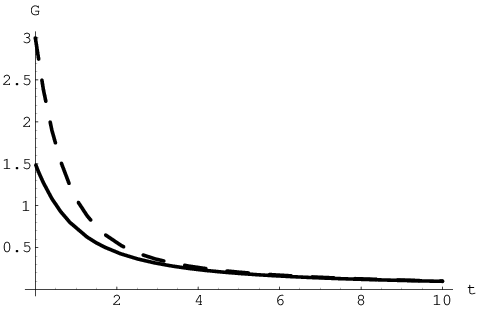
The above discretization is handy if the relaxation measure $\mu$ and the function $\mathsf{H}$ are known The quadrature depends only on the measure $\mu$ because the function $\mathsf{H}$ is bounded on the support of $\mu$. The quadrature can often be evaluated with a few nodes instead of a long and growing number of memory points if a Grünwald-Letnikov discretization is applied. If the relaxation spectrum is unbounded then asymptotic estimates of the integrand can be helpful. In some cases the relaxation spectrum can be finite, for example if $\mu(\mathrm{d}r)=\theta(\Omega-r)\,(1-r/\Omega)^{\alpha}$, $\alpha>-1$, $\Omega>0$. Assuming that $\mathsf{H}(r)=\mathbf{Id}_{S}$, the relaxation modulus is a LICM function $\mathsf{G}(t)=g(t)\,\mathrm{Id}_{S}$ with $g(t)=\Omega\,\mathrm{e}^{-\Omega\,t}(-\Omega t)^{-1-\alpha}\,[\Gamma(\alpha)-\Gamma(\alpha,-\Omega t)]$ (the two factors are complex valued, but the product is real valued). For $\alpha=0.5$ $g(t)=2/3\,\mathrm{e}^{-\Omega t}\,_{1}F_{1}(1.5,2.5,\Omega t)$ and for $\alpha=-0.5$ $g(t)=2\,\mathrm{e}^{-\Omega t}\,_{1}F_{1}(0.5,1.5,\Omega t)$. For $\alpha=\pm 1/3$ the functions are shown in Fig. 1.

The integral over the relaxation spectrum $[0,\Omega]$ can be expressed in terms of the Gauss-Jacobi quadrature on $[-1,1]$ [21] by the formula

$$\int_{0}^{\Omega}(1-\Omega/r)^{\alpha}\,f(r)\,\mathrm{d}r=\Omega\,2^{-1-\alpha}\int_{-1}^{1}(1-x)^{\alpha}\,f(\Omega\,(x+1)/2)\,\mathrm{d}x$$

The quadrature nodes and weights can be calculated by the method presented in op. cit.

The relaxation spectral measures of several viscoelastic models of practical interest are presented in [5, 6]. These include the Cole-Cole, Havriliak-Negami, Cole-Davidson models and Prony sums.

We shall show how the convolution operator can be eliminated/replaced by a quadrature. The method is applicable to viscoelastic media with a separable relaxation modulus

$$\mathsf{G}(s,\mathbf{x})=g(s)\,\mathsf{C}(\mathbf{x})$$

(14)

where $\mathsf{C}(\mathbf{x})$ is positive semi-definite symmetric operator on $S$, invertible for every $\mathbf{x}\in\mathcal{U}$ and $g$ is a LICM function. In this case equation (6) is satisfied by $\mathsf{J}(s,\mathbf{x})=j(s)\,\mathsf{C}(\mathbf{x})^{-1}$, where $j(t)$ is the unique solution of the equation

$$\int_{0}^{t}j(s)\,g(t-s)\,\mathrm{d}s=t\qquad t>0$$

(15)

The function $j$ is non-decreasing and non-negative, hence it has a finite limit $j(0+)\geq 0$ as $t\rightarrow 0$. This limit is non-zero if $\lim_{t\rightarrow 0}g(t)<\infty$. In this case $j(0+)=1/g(0+)$ [10].

Equation (14) means that the memory effects are independent of the material point and of the direction in an anisotropic medium. The anisotropy is entirely accounted for by the tensor $\mathsf{C}(\mathbf{x})$. This condition is satisfied in particular by the shear flow of an isotropic viscoelastic medium. In this case $d=1$, $\mathbf{x}$ reduces to a single coordinate $x$, while $\mathbf{u}$ reduces to a component $u_{y}$ of $\mathbf{u}$ orthogonal to the $x$ direction. The tensor $\mathsf{C}$ can be set equal to 1 and $g(t)$ plays the role of the viscoelastic shear relaxation modulus, with $g(0)=\mu$ – the Lamé elastic shear modulus.

Assuming separability of the relaxation modulus, equation (2) reduces to

$$\rho\,\mathbf{u}^{\prime\prime}(t,\mathbf{x})=g\ast L\left[\mathbf{u}^{\prime}\right]+\mathbf{f}(t,\mathbf{x})$$

(16)

where $L[\mathbf{u}]:=\nabla\cdot\{\mathsf{C}(\mathbf{x})[\nabla\,\mathbf{u}(t,\mathbf{x})]\}$.

We shall now eliminate the convolution operator $g\ast$ by applying the convolution operator $j\ast$ to both sides of equation (16). Using equation (15) we obtain the equation

$$\rho\,j\ast\mathbf{u}^{\prime\prime}=t\ast L[\mathbf{u}^{\prime}]+j\ast\mathbf{f}(t,\mathbf{x})$$

(17)

The Fubini theorem implies the identity

$$\int_{0}^{t}\left[\int_{0}^{s}f(\xi)\,\mathrm{d}\xi\right]\,\mathrm{d}s=\int_{0}^{t}(t-\xi)\,f(\xi)\,\mathrm{d}\xi$$

Using this identity equation (17) can be transformed to the following form

$$\rho\,j\ast\mathbf{u}^{\prime\prime}=\int_{0}^{t}L[\mathbf{u}(s,\mathbf{x})-\mathbf{u}(0,\mathbf{x})]\,\mathrm{d}s+j\ast\mathbf{f}$$

Differentiating the last equation with respect to time and noting the identity

$$\partial\left[j\ast\mathbf{u}^{\prime\prime}\right]/\partial t=\partial\int_{0}^{t}j(t-s)\,\mathbf{u}^{\prime\prime}(s,\mathbf{x})\,\mathrm{d}s/\partial t=j(0)\,\mathbf{u}^{\prime\prime}+j^{\prime}\ast\mathbf{u}^{\prime\prime}$$

we get the equation

$$j(0+)\,\mathbf{u}^{\prime\prime}+j^{\prime}\ast\mathbf{u}^{\prime\prime}=L[\mathbf{u}(t,\mathbf{x})-\mathbf{u}(0,\mathbf{x})]+j(0+)\,\mathbf{f}(t,\mathbf{x})+j^{\prime}\ast\mathbf{f}$$

(18)

Recall Bernstein’s theorem for the LICM function $j^{\prime}$ [18]:

$$j^{\prime}(s)=\int_{[0,\infty[}\mathrm{e}^{-rs}\,\nu(\mathrm{d}r)$$

(19)

where $\nu$ is a positive Radon measure on $[0,\infty[$ satisfying the inequality

$$\int_{[0,\infty[}\frac{\nu(\mathrm{d}r)}{1+r}<\infty$$

(20)

The convolution $j^{\prime}\ast\mathbf{u}^{\prime\prime}$ can now be expressed in terms of an integral over $[0,\infty[$:

$$\left[j^{\prime}\ast\mathbf{u}^{\prime\prime}\right](t,\mathbf{x})=\int_{[0,\infty[}\mathbf{\phi}_{r}(t,\mathbf{x})\,\nu(\mathrm{d}r)$$

(21)

where

$$\mathbf{\phi}_{r}(t,\mathbf{x}):=\int_{0}^{t}\mathrm{e}^{-r(t-s)}\,\mathbf{u}^{\prime\prime}(s,\mathbf{x})\,\mathrm{d}s$$

(22)

Note that $\mathbf{\phi}_{r}$ can be calculated simultaneously with $\mathbf{u}$ by integrating the differential equations

$$\mathbf{\phi}_{r}^{\;\prime}+r\,\mathbf{\phi}_{r}-\mathbf{u}^{\prime\prime}=0\qquad r\geq 0$$

(23)

with the initial condition $\mathbf{\phi}_{r}(0,\mathbf{x})=0$.

We thus end up with the equation

$$\rho\,j(0+)\,\mathbf{u}^{\prime\prime}+\int_{[0\infty[}\mathbf{\phi}_{r}(t,\mathbf{x})\,\nu(\mathrm{d}r)=L[\mathbf{u}(t,\mathbf{x})-\mathbf{u}(0,\mathbf{x})]+j(0+)\,\mathbf{f}(t,\mathbf{x})+j^{\prime}\ast\mathbf{f}$$

(24)

The integral on the left-hand side is convergent. Indeed

$$r\,\|\mathbf{\phi}_{r}(t,\mathbf{x})\|\leq\int_{0}^{t}r\,\mathrm{e}^{-r(t-s)}\,\|\,\mathbf{u}^{\prime\prime}(s,\mathbf{x})\|\,\mathrm{d}s$$

The integrand on the right tends to 0 as $r\rightarrow\infty$ for $0\leq s<t$, hence almost everywhere on $[0,t]$. If $\sup_{0\leq s\leq t}\|\mathbf{u}^{\prime\prime}(s,\mathbf{x})\|<C<\infty$ then the integrand is bounded and integrable on $[0,t]$. By the Lebesgue Dominated Convergence Theorem $\lim_{r\rightarrow\infty}r\,\mathbf{\phi}_{r}(t,\mathbf{x})=0$ and in view of (20) the integral in equation (24) is convergent.

Suppose that the second term on the left-hand side of equation (24) can be approximated by a quadrature with nodes $r_{l}$ and weights $w_{l}$, $l=1,\ldots,n$, independent of $t,\mathbf{x}$:

$$\int_{[0\infty[}\mathbf{\phi}_{r}(t,\mathbf{x})\,\nu(\mathrm{d}r)\sim\sum_{l=1}^{n}w_{l}\,\mathbf{\phi}_{r_{l}}(t,\mathbf{x})$$

(25)

and let $\mathbf{\psi}_{l}(t,\mathbf{x}):=\mathbf{\phi}_{r_{l}}(t,\mathbf{x})$ for $l=1,\ldots,n$. The original IVP can be approximated by the equations

	$$\displaystyle\rho\,j(0+)+\sum_{l=1}^{n}w_{l}\,\mathbf{\psi}_{l}=L[\mathbf{u}]+j(0+)\,\mathbf{f}(t,\mathbf{x})+j^{\prime}\ast\mathbf{f}\qquad t\geq 0,\quad\mathbf{x}\in\mathcal{U}$$		(26)
	$$\displaystyle\mathbf{\psi}_{l}^{\;\prime}+r_{l}\,\mathbf{\psi}_{l}-\mathbf{u}^{\prime\prime}=0\qquad l=1,\ldots,n;\;t\geq 0;\;\mathbf{x}\in\mathcal{U}$$		(27)
	$$\displaystyle\mathbf{u}(0,\mathbf{x})=0;\;\mathbf{u}^{\prime}(0,\mathbf{x})=0;\;\mathbf{\psi}_{l}(0,\mathbf{x})=0\qquad\mathbf{x}\in\mathcal{U}$$		(28)
	$$\displaystyle\mathbf{u}(t,\mathbf{x})=0\qquad\mathbf{x}\in[0,\infty[\,\times\Gamma_{1}$$		(29)
	$$\displaystyle\mathbf{n}\cdot\mathsf{C}(\mathbf{x})[\nabla\,\mathbf{u}(t,\mathbf{x})]=0\qquad\mathbf{x}\in[0,\infty[\,\times\Gamma_{2}$$		(30)

Discretize the time according to the formula $t=m\,h$, where $h>0$ is a step size, and let $\mathbf{u}_{m}(\mathbf{x}):=\mathbf{u}(m\,h,\mathbf{x})$, $\mathbf{u}^{\prime\prime}_{m}(\mathbf{x}):=\mathbf{u}^{\prime\prime}(m\,h,\mathbf{x})$, $\psi_{l,m}(\mathbf{x}):=\psi_{l}(m\,h,\mathbf{x})$. Suppose that $\mathbf{u}_{k},\psi_{l,k}$ has been calculated for $k\leq m$, $1\leq l\leq n$. According to a tentative numerical scheme equation (26) can be used do calculate $\mathbf{u}^{\prime\prime}_{m}$. Equations (27) can be used to calculate $\psi_{l,m+1}$, while $\mathbf{u}_{m},\mathbf{u}_{m-1}$ and $\mathbf{u}^{\prime\prime}_{m}$ can be used to calculate $\mathbf{u}_{m+1}$.

The Radon measure $\nu$ can be expressed in terms of the retardation measure [10]. Apply the general integral representation of a Bernstein function to $j(t)$ [18]:

$$j(s)=j(0+)+s\,N+\int_{]0,\infty[}\left[1-\mathrm{e}^{-rs}\right]\,\mu(\mathrm{d}r)$$

(31)

where the retardation measure $\mu$ is a positive Radon measure on $]0,\infty[$ satisfying the inequality

$$\int_{]0,\infty[}\frac{r\,\mu(\mathrm{d}r)}{1+r}<\infty$$

(32)

Equation (31) implies equation (19) with $\nu(\mathrm{d}r)=r\,\mu(\mathrm{d}r)$ for $r>0$ and $\nu\{0\}=N$. Equation (32) implies equation (20).

The method presented in Section 4 is particularly effective if the retardation spectrum, i. e. the support of the measures $\mu$ and $\nu$ is a finite interval. This is in particular the case for the Strick-Mainardi creep compliance $j(t)$, defined by its Laplace transform

$$\tilde{j}(p)=J_{0}+M_{0}\,\left[(1+\Omega/p)^{\alpha}-1\right]/\alpha$$

(33)

where $J_{0},M_{0}$ and $\Omega$ are some positive constants and $0<\alpha<1$. The Radon measure $\nu$ is given by the formula $\nu(\mathrm{d}r)=W(r)\,\mathrm{d}r$, where $W(r):=\Im\left[\widetilde{J^{\prime}}\left(r\,\mathrm{e}^{-\mathrm{i}\uppi}\right)\right]/\uppi$ which in our particular case is given by the formula is

$$W(r)=\begin{cases}M_{0}\frac{\sin(\alpha\,\uppi)}{\alpha\uppi}\left(\Omega/p-1\right)^{\alpha}&r\leq\Omega\\ 0&r>\Omega\end{cases}$$

(34)

for $r\geq 0$. Hence

$$j^{\prime}\ast\mathbf{u}^{\prime\prime}=\int_{0}^{\Omega}W(r)\,\mathbf{\phi}_{r}(t,\mathbf{x})\,\mathrm{d}r$$

The retardation spectrum is the interval $[0,\Omega]$. The convolution

$$j^{\prime}\ast\mathbf{u}^{\prime\prime}(t,\mathbf{x})=M_{0}\,\Omega\,\int_{-1}^{1}(1-\xi)^{\alpha}\,(1+\xi)^{-\alpha}\mathbf{\phi}_{\Omega\,(1+\xi)/2}(t,\mathbf{x})\,\mathrm{d}\xi$$

(35)

can be approximated by Gauss-Jacobi quadrature [21]:

$$j^{\prime}\ast\mathbf{u}^{\prime\prime}(t,\mathbf{x})=M_{0}\,\Omega\,\frac{\sin(\alpha\uppi)}{\alpha\uppi}\sum_{l=1}^{n}w_{l}\,\mathbf{\phi}_{\Omega(1+\xi_{l})/2}(t,\mathbf{x})$$

(36)

where the nodes $\xi_{l}$, $l=1,\ldots,n$ are the roots of a Jacobi polynomial of degree $n$ and $w_{l}$, $l=1,\ldots,n$, are the corresponding weights [20, 8]. The nodes $\xi_{l}$ and the weights $w_{l}$ can be calculated by the programs presented in Sec. 2.5 of [21].

A numerical approximation of the operator $L[\mathbf{u}]$ can be constructed by the FEM [19] or the pseudospectral method [4].

Numerial integration of equations involving memory effects normally requires multiplications and summations of an ever increasing sequence of past values of each physical variable. The proposed method is based on the idea of auxiliary variables which contain the information relevant for the future evolution of the system. There is a continuum of such variables and their contributions should be summed with appropriate weights. The resulting integral can however be much easier to calculate than the time convolution of memory dependent variables.

In many cases the retardation spectrum is infinite. In the case of an infinite retardation spectrum the integration domain can be mapped to a finite interval by a Cayley transformation. the quadrature can also be reduced to a few nodes by applying an asymptotic estimate of the integrand [9].

A Caputo fractional derivative of order $\alpha\in]0,1]$ is given by the formula $\mathrm{D}^{\alpha}f=\int_{0}^{t}\frac{s^{-\alpha}}{\Gamma(1-\alpha)}f^{\prime}(t-s)\,\mathrm{d}s$ [17] and $s^{-\alpha}/\Gamma(1-\alpha)$ is a LICM function. It is therefore possible to apply similar methods to equations with fractional derivatives.

In particular a viscoelastic medium can be defined in terms of Caputo fractional derivatives. This approach to hereditary viscoelasticity has a long history associated with the names of Gemant, Scott-Blair, Rabotnov, Caputo and Koeller. A detailed account of this class of viscoelastic models can be found in [14]. We shall now relate these models to the models based on completely monotonic relaxation moduli and Bernstein creep compliances [1, 15, 10]. If the creep compliance is given by the formula $j(s)=M_{0}\,s^{1-\alpha}/\Gamma(2-\alpha)$ then the convolution $j^{\prime}\ast\mathbf{u}^{\prime\prime}=M_{0}\,\mathrm{D}^{\alpha+1}\mathbf{u}$ is a Caputo derivative. Equation (18) assumes the form

$$j(0+)\,\mathbf{u}^{\prime\prime}+M_{0}\,\mathrm{D}^{\alpha+1}\,\mathbf{u}=L[\mathbf{u}(t,\mathbf{x})-\mathbf{u}(0,\mathbf{x})]+j(0+)\,\mathbf{f}(t,\mathbf{x})+j^{\prime}\ast\mathbf{f}$$

In this case $j^{\prime}(s)=s^{-\alpha}/\Gamma(1-\alpha)=\int_{0}^{\infty}\mathrm{e}^{-rt}\,r^{\alpha-1}/\Gamma(\alpha)\mathrm{d}r$, hence the retardation spectrum is infinite and $W(r)=r^{\alpha-1}/\Gamma(\alpha)$. Equation (6) in the Laplace domain assumes the form $\tilde{j}(p)\,\tilde{g}(p)=p^{-2}$ with $\tilde{j}(p)=p^{\alpha-2}$, hence $\tilde{g}(p)=p^{-\alpha}$ and $g(s)=s^{\alpha-1}/\Gamma(\alpha)$. Consequently the constitutive equation assumes the form $\upsigma(t,\mathbf{x})=\mathrm{D}^{1-\alpha}\mathsf{C}(\mathbf{x})[\nabla\mathbf{u}]$.

References

- [1] D. R. Bland, The Theory of Linear Viscoelasticity. Pergamon Press, Oxford 1960.
- [2] K. Diethelm, An investigation of some non-classical methods for numerical approximation of Caputo-type fractional derivatives Numer. Algor. 47:361–390 2008
- [3] K. Diethelm, The Analysis of Fractional Differential Equations. Springer, Heidelberg 2010.
- [4] B. Fornberg, A practical Guide to Pseudospectral Methods. Cambridge University Press, Cambridge 1996.
- [5] M. Seredyńska and A. Hanyga Relaxation, dispersion, attenuation and finite propagation speed in viscoelastic media J. Math. Phys. 51:092901–092916 2010.
- [6] A. Hanyga Wave propagation in linear viscoelastic media with completely monotonic relaxation moduli Wave Motion 50:909–928 2013.
- [7] A. Hanyga Multi-dimensional solutions of space-time fractional diffusion equations Proc. Roy. Soc. A 458:429–450 2002.
- [8] A. Hanyga, Attenuation and shock waves in linear hereditary viscoelastic media; Strick-Mainardi, Jeffreys-Lomnitz-Strick and Andrade creep compliances. Pure and Appl. Geophysics 1–13 2014.
- [9] A. Hanyga and J.-F. Lu, Wave simulation for heterogeneous transversely isotropic porous media with the JKD dynamic permeability. Comput. Mech. 36:196–208 2005.
- [10] A. Hanyga and M. Seredyńska, Relations between the relaxation modulus and the creep compliance in anisotropic linear viscoelastic medium. J. of Elasticity 88:41–61 2007.
- [11] J.-F Lu and A. Hanyga, Numerical modeling method for wave propagation in a linear viscoelastic medium with a singular memory. Geophys. J. Int. 159:688–702 2004.
- [12] J.-F Lu and A. Hanyga, Fundamental solution for a layered porous half-space subject to a vertical point source or a point fluid force. Comput. Mech. 35:376–391 2005
- [13] J.-F Lu and A. Hanyga, Wavefield simulation for heterogeneous porous media with a singular drag force. J. Comp. Phys. 208:651–674 2005.
- [14] F. Mainardi, Fractional Calculus and Waves in Linear Viscoelasticity. Imperial College Press, london 2010.
- [15] A. Molinari, Viscoélasticité linéaire et fonctions complètement monotones. J. de mécanique 12:541–553 1975.
- [16] G. Montsény, Diffusive representation of pseudo-differential time operators. In ESAIM Proceedings, vol. 5, pp 159–175, 1998.
- [17] I. Podlubny Fractional Differential Equations. Academic Press, San Diego 1999.
- [18] R. L. Schilling, R. Song and Z. Vondraek, Bernstein Functions. Theory and Applications. DE Gruyter, Berlin 2010.
- [19] G. Strang and G. J. Fix, An Analysis of the Finite Element Method. Prentice-Hall Inc., Englewood Cliffs, N. J., 1974.
- [20] E. Strick and F. Mainardi, On a general class of constant solids. Geophys. J. Roy. astr. Soc. 69:415–429 1982.
- [21] A. H. Stroud and D. Secrest, Gaussian Quadrature Formulas. Prentice-Hall Inc., London, 1966.
- [22] L. Yuan and O. P. Agrawal, A numerical scheme for for dynamic systems containing fractional derivatives In ”Proc. of the DETC ’98 ASME Design Engineering Technical Conferences, Sept. 13–16, 1998”, Atlanta, GA, 1998.